Estimation and Inference for Minimizer and Minimum of Convex Functions: Optimality, Adaptivity, and Uncertainty Principles

Abstract

Optimal estimation and inference for both the minimizer and minimum of a convex regression function under the white noise and nonparametric regression models are studied in a non-asymptotic local minimax framework, where the performance of a procedure is evaluated at individual functions. Fully adaptive and computationally efficient algorithms are proposed and sharp minimax lower bounds are given for both the estimation accuracy and expected length of confidence intervals for the minimizer and minimum.

The non-asymptotic local minimax framework brings out new phenomena in simultaneous estimation and inference for the minimizer and minimum. We establish a novel Uncertainty Principle that provides a fundamental limit on how well the minimizer and minimum can be estimated simultaneously for any convex regression function. A similar result holds for the expected length of the confidence intervals for the minimizer and minimum.

, , and

1 Introduction

Motivated by a range of applications, estimation of and inference for the location and size of the extremum of a nonparametric regression function has been a longstanding problem in statistics. See, for example, Kiefer and Wolfowitz, (1952); Blum, (1954); Chen, (1988). The problem has been investigated in different settings. For fixed design, upper bounds for estimating the minimum over various smoothness classes have been obtained (Muller,, 1989; Facer and Müller,, 2003; Shoung and Zhang,, 2001). Belitser et al., (2012) establishes the minimax rate of convergence over a given smoothness class for estimating both the minimizer and minimum. For sequential design, the minimax rate for estimation of the location has been established; see Chen et al., (1996); Polyak and Tsybakov, (1990); Dippon, (2003). Mokkadem and Pelletier, (2007) introduces a companion for the Kiefer–Wolfowitz–Blum algorithm in sequential design for estimating both the minimizer and minimum.

Another related line of research is the stochastic continuum-armed bandits, which have been used to model online decision problems under uncertainty. Applications include online auctions, web advertising and adaptive routing. Stochastic continuum-armed bandits can be viewed as aiming to find the maximum of a nonparametric regression function through a sequence of actions. The objective is to minimize the expected total regret, which requires the trade-off between exploration of new information and exploitation of historical information. See, for example, Kleinberg, (2004); Auer et al., (2007); Kleinberg et al., (2019).

In the present paper, we consider optimal estimation and confidence intervals for the minimizer and minimum of convex functions under both the white noise and nonparametric regression models in a non-asymptotic local minimax framework that evaluates the performance of any procedure at individual functions. This framework provides a much more precise analysis than the conventional minimax theory, which evaluates the performance of the estimators and confidence intervals in the worst case over a large collection of functions. This framework also brings out new phenomena in simultaneous estimation and inference for the minimizer and minimum.

We first focus on the white noise model, which is given by

$$\mathrm{d}Y(t)=f(t)\mathrm{d}t+\varepsilon\mathrm{d}W(t),\quad 0\leq t\leq 1,$$ (1.1)

where $W(t)$ is a standard Brownian motion, and $\varepsilon>0$ is the noise level. The drift function $f$ is assumed to be in ${\mathcal{F}}$, the collection of convex functions defined on $[0,1]$ with a unique minimizer ${\color[rgb]{0,0,0}Z(f)}=\operatorname*{\arg\min}_{0\leq t\leq 1}f(t)$. The minimum value of the function $f$ is denoted by $M(f)$, i.e., ${\color[rgb]{0,0,0}M(f)}=\min_{0\leq t\leq 1}f(t)=f({\color[rgb]{0,0,0}Z(f)})$. The goal is to optimally estimate ${\color[rgb]{0,0,0}Z(f)}$ and ${\color[rgb]{0,0,0}M(f)}$, as well as construct optimal confidence intervals for ${\color[rgb]{0,0,0}Z(f)}$ and ${\color[rgb]{0,0,0}M(f)}$. Estimation and inference for the minimizer ${\color[rgb]{0,0,0}Z(f)}$ and minimum ${\color[rgb]{0,0,0}M(f)}$ under the nonparametric regression model will be discussed later in Section 4.

1.1 Function-specific Benchmarks and Uncertainty Principle

As the first step toward evaluating the performance of a procedure at individual convex functions in ${\mathcal{F}}$, we define the function-specific benchmarks for estimation of the minimizer and minimum respectively by

$$R_{z}(\varepsilon;f) =\sup_{g\in{\mathcal{F}}}\inf_{\hat{Z}}\max_{h\in\{f,g\}}\mathbb{E}_{h}|\hat{Z}-Z(h)|,$$ (1.2)

$$R_{m}(\varepsilon;f) =\sup_{g\in{\mathcal{F}}}\inf_{\hat{M}}\max_{h\in\{f,g\}}\mathbb{E}_{h}|\hat{M}-M(h)|.$$ (1.3)

As in (1.2) and (1.3), we use subscript ‘$z$’ to denote quantities related to the minimizer and ‘$m$’ for the minimum throughout the paper. For any given $f\in{\mathcal{F}}$, the benchmarks $R_{z}(\varepsilon;f)$ and $R_{m}(\varepsilon;f)$ quantify the estimation accuracy at $f$ of the minimizer ${\color[rgb]{0,0,0}Z(f)}$ and minimum ${\color[rgb]{0,0,0}M(f)}$ against the hardest alternative to $f$ within the function class ${\mathcal{F}}$.

We show that $R_{z}(\varepsilon;f)$ and $R_{m}(\varepsilon;f)$ are the right benchmarks for capturing the estimation accuracy at individual functions in ${\mathcal{F}}$ and will construct adaptive procedures that simultaneously perform within a constant factor of $R_{z}(\varepsilon;f)$ and $R_{m}(\varepsilon;f)$ for all $f\in{\mathcal{F}}$. In addition, it is also shown that any estimator $\hat{Z}$ for the minimizer that is “super-efficient” at some $f_{0}\in{\mathcal{F}}$, i.e., it significantly outperforms the benchmark $R_{z}(\varepsilon;f_{0})$, must pay a penalty at another function $f_{1}\in{\mathcal{F}}$ and thus no procedure can uniformly outperform the benchmark. An analogous result holds for the minimum.

More interestingly, the non-asymptotic local minimax framework enables us to establish a novel Uncertainty Principle for estimating the minimizer and minimum of a convex function. The Uncertainty Principle reveals an intrinsic tension between the task of estimating the minimizer and that of estimating the minimum. That is, there is a fundamental limit to the estimation accuracy of the minimizer and minimum for all functions in ${\mathcal{F}}$ and consequently the minimizer and minimum of a convex function cannot be estimated accurately at the same time. More specifically, it is shown that

$$R_{z}(\varepsilon;f)\cdot R_{m}(\varepsilon;f)^{2}\asymp\varepsilon^{2}$$ (1.4)

for all $f\in{\mathcal{F}}$. Further, on the lower bound side,

$$\inf_{f\in{\mathcal{F}}}R_{z}(\varepsilon;f)\cdot R_{m}(\varepsilon;f)^{2}\geq{\Phi(-0.5)^{3}\over 2}\varepsilon^{2},$$ (1.5)

where $\Phi(\cdot)$ is the cumulative distribution function (cdf) of the standard normal distribution.

For confidence intervals with a pre-specified coverage probability, the hardness of the problem is naturally characterized by the expected length. Let $\mathcal{I}_{z,\alpha}({\mathcal{F}})$ and $\mathcal{I}_{m,\alpha}({\mathcal{F}})$ be, respectively, the collection of confidence intervals for the minimizer ${\color[rgb]{0,0,0}Z(f)}$ and the minimum ${\color[rgb]{0,0,0}M(f)}$ with guaranteed coverage probability $1-\alpha$ for all $f\in{\mathcal{F}}$. Let $L(CI)$ be the length of a confidence interval $CI$. The minimum expected lengths at $f$ of all confidence intervals in $\mathcal{I}_{z,\alpha}(\{f,g\})$ and $\mathcal{I}_{m,\alpha}(\{f,g\})$ with the hardest alternative $g\in{\mathcal{F}}$ for $f$ are given by

$$L_{z,\alpha}(\varepsilon;f) =\sup_{g\in{\mathcal{F}}}\inf_{CI\in\mathcal{I}_{z,\alpha}(\{f,g\})}\mathbb{E}_{f}L(CI),$$ (1.6)

$$L_{m,\alpha}(\varepsilon;f) =\sup_{g\in{\mathcal{F}}}\inf_{CI\in\mathcal{I}_{m,\alpha}(\{f,g\})}\mathbb{E}_{f}L(CI).$$ (1.7)

As in the case of estimation, we will first evaluate these benchmarks for the performance of confidence intervals in terms of the local moduli of continuity and then construct data-driven and computationally efficient confidence interval procedures. Furthermore, we also establish the Uncertainty Principle for the confidence intervals,

$$\inf_{f\in{\mathcal{F}}}L_{z,\alpha}(\varepsilon;f)\cdot L_{m,\alpha}(\varepsilon;f)^{2}\geq C_{\alpha}\varepsilon^{2}.$$ (1.8)

where $C_{\alpha}$ is a positive constant depending on $\alpha$ only. The Uncertainty Principle (1.8) shows a fundamental limit for the accuracy of simultaneous inference for the minimizer ${\color[rgb]{0,0,0}Z(f)}$ and minimum ${\color[rgb]{0,0,0}M(f)}$ for any $f\in{\mathcal{F}}$.

1.2 Adaptive Procedures

Another major step in our analysis is developing data-driven and computationally efficient algorithms for the construction of adaptive estimators and adaptive confidence intervals as well as establishing the optimality of these procedures at each $f\in{\mathcal{F}}$.

The key idea behind the construction of the adaptive procedures is to iteratively localize the minimizer by computing the integrals over the relevant subintervals together with a carefully constructed stopping rule. For estimation of the minimum and minimizer, additional estimation procedures are added after the localization steps. For the construction of the confidence intervals, another important idea is to look back a few steps before the stopping time.

The resulting estimators, ${\color[rgb]{0,0,0}\hat{Z}}$ for the minimizer ${\color[rgb]{0,0,0}Z(f)}$ and ${\color[rgb]{0,0,0}\hat{M}}$ for the minimum ${\color[rgb]{0,0,0}M(f)}$, are shown to attain within a constant factor of the benchmarks $R_{z}(\varepsilon;f)$ and $R_{m}(\varepsilon;f)$ simultaneously for all $f\in{\mathcal{F}}$,

$$\mathbb{E}_{f}|{\color[rgb]{0,0,0}\hat{Z}-Z(f)}|\leq C_{z}R_{z}(\varepsilon;f)\quad{\rm and}\quad\mathbb{E}_{f}|{\color[rgb]{0,0,0}\hat{M}-M(f)}|\leq C_{m}R_{m}(\varepsilon;f),\\$$

for some absolute constants $C_{z}$ and $C_{m}$ not depending on $f$. The confidence intervals, $CI_{z,\alpha}$ for the minimizer ${\color[rgb]{0,0,0}Z(f)}$ and $CI_{m,\alpha}$ for the minimum ${\color[rgb]{0,0,0}M(f)}$, are constructed and shown to be adaptive to individual functions $f\in{\mathcal{F}}$, while having guaranteed coverage probability $1-\alpha$. That is, $CI_{z,\alpha}\in\mathcal{I}_{z,\alpha}({\mathcal{F}})$ and $CI_{m,\alpha}\in\mathcal{I}_{m,\alpha}({\mathcal{F}})$ and for all $f\in{\mathcal{F}}$,

$$\mathbb{E}_{f}L(CI_{z,\alpha}) \leq C_{z}(\alpha)L_{z,\alpha}(\varepsilon;f)$$

$$\mathbb{E}_{f}L(CI_{m,\alpha}) \leq C_{m}(\alpha)L_{m,\alpha}(\varepsilon;f),$$

where $C_{z}(\alpha)$ and $C_{m}(\alpha)$ are constants depending on $\alpha$ only.

1.3 Related Literature

In addition to estimation and inference for the location and size of the extremum of a nonparametric regression function mentioned at the beginning of this section, the problems considered in the present paper are also connected to nonparametric estimation and inference under shape constraints, which have also been well studied in the literature.

Nonparametric convex regression has been investigated in various settings, ranging from estimation and confidence bands for the whole function (Birge,, 1989; Guntuboyina and Sen,, 2018; Hengartner and Stark,, 1995; Dumbgen,, 1998), to estimation and inference at a fixed point (Kiefer,, 1982; Cai et al.,, 2013; Cai and Low,, 2015; Ghosal and Sen,, 2017). Deng et al., (2020) established limiting distributions for some local parameters of a convex regression function, including the minimizer based on the convexity-constrained least squares (CLS) estimator and constructed a confidence interval for the minimizer. As seen in Section 4.4 and further discussions in the Supplementary Material (Cai et al.,, 2021, Section LABEL:subsec:ci_subopt), this confidence interval is suboptimal in terms of the expected length under the local minimax framework that we will introduce later. It is also much more computationally intensive as it requires solving the CLS problem.

In the context of estimating and inferring the value of a convex function at a fixed point, which is a linear functional, the local minimax framework characterized by the benchmarks (1.2)-(1.3) and (1.6)-(1.7) has been used in Cai et al., (2013) and Cai and Low, (2015). However, the focus of the present paper is on the minimizer and minimum, which are nonlinear functionals. Due to their nonlinear nature, the analysis is much more challenging than it is for the function value at a fixed point.

Another related line of research is stochastic numerical optimization of convex functions. Agarwal et al., (2011) studies stochastic convex optimization with bandit feedback and proposes an algorithm that is shown to be nearly minimax optimal. Chatterjee et al., (2016) uses the framework introduced in Cai and Low, (2015) to study the local minimax complexity of stochastic convex optimization based on queries to a first-order oracle that produces an unbiased subgradient in a rather restrictive setting.

1.4 Organization of the Paper

In Section 2, we analyze individual minimax risks, relating them to appropriate local moduli of continuity and more explicit alternative expressions, and explain the uncertainty principle with a discussion of the connections with the classical minimax framework. Super-efficiency is also considered. In Section 3, we introduce the adaptive procedures for the white noise model and show that they are optimal. In Section 4, we consider the nonparametric regression model. Adaptive procedures are proposed and their optimality is established. In addition, a summary of the numerical results is given. Section 5 discusses some future directions. Two main theorems are proved in Section 6. For reasons of space, the proofs of other results are given in the Supplementary Material Cai et al., (2021).

1.5 Notation

We finish this section with some notation that will be used in the rest of the paper. The cdf of the standard normal distribution is denoted by $\Phi$. For $0<\alpha<1$, $z_{\alpha}=\Phi^{-1}(1-\alpha)$. For two real numbers $a$ and $b$, $a\wedge b=\min\{a,b\}$, $a\vee b=\max\{a,b\}$. $\|\cdot\|_{2}$ denotes the $L_{2}$ norm (i.e., $\|f\|_{2}=\sqrt{\int f(x)^{2}\mathrm{d}x}$ ). For $f\in L_{2}[0,1]$ and $r>0$, $\mathcal{B}_{r}(f)=\{g\in L_{2}[0,1]:\|g-f\|_{2}\leq r\}$ and $\partial{\mathcal{B}_{r}}(f)=\{g\in L_{2}[0,1]:\|g-f\|_{2}=r\}$.

2 Benchmarks and Uncertainty Principle

In this section, we first introduce the local moduli of continuity and use them to characterize the four benchmarks for estimation and confidence intervals introduced in Section 1.1, which are summarized in the following table:

	Estimation	Inference
Minimizer ${\color[rgb]{0,0,0}Z(f)}$	$R_{z}(\varepsilon;f)$	$L_{z,\alpha}(\varepsilon;f)$
Minimum ${\color[rgb]{0,0,0}M(f)}$	$R_{m}(\varepsilon;f)$	$L_{m,\alpha}(\varepsilon;f)$.

We provide alternative expressions for the local moduli of continuity that are easier to evaluate. The results are used to establish a novel Uncertainty Principle, which shows an intrinsic tension between the estimation/inference accuracy for the minimizer and the minimum for all functions in ${\mathcal{F}}$.

2.1 Local Moduli of Continuity

For any given convex function $f\in{\mathcal{F}}$, we define the following local moduli of continuity, one for the minimizer, and the other for the minimum,

$$\omega_{z}(\varepsilon;f) = \sup\left\{|{\color[rgb]{0,0,0}Z(f)-Z(g)}|:\|f-g\|_{2}\leq\varepsilon,\,g\in{\mathcal{F}}\right\},$$ (2.1)

$$\omega_{m}(\varepsilon;f) = \sup\left\{|{\color[rgb]{0,0,0}M(f)-M(g)}|:\|f-g\|_{2}\leq\varepsilon,\,g\in{\mathcal{F}}\right\},$$ (2.2)

As in the case of a linear functional, the local moduli $\omega_{z}(\varepsilon;f)$ and $\omega_{m}(\varepsilon;f)$ clearly depend on the function $f$ and can be regarded as an analogue of the inverse Fisher Information in regular parametric models.

The following theorem characterizes the four benchmarks for estimation and inference in terms of the corresponding local modulus of continuity.

Theorem 2.1.

Let $0<\alpha<0.3$. Then

$$a_{1}\omega_{z}(\varepsilon;f)\leq R_{z}(\varepsilon;f) \leq A_{1}\omega_{z}(\varepsilon;f),$$ (2.3)

$$a_{1}\omega_{m}(\varepsilon;f)\leq R_{m}(\varepsilon;f) \leq A_{1}\omega_{m}(\varepsilon;f),$$ (2.4)

$$b_{\alpha}\omega_{z}(\varepsilon/3;f)\leq L_{z,\alpha}(\varepsilon;f) \leq B_{\alpha}\omega_{z}(\varepsilon;f),$$ (2.5)

$$b_{\alpha}\omega_{m}(\varepsilon/3;f)\leq L_{m,\alpha}(\varepsilon;f) \leq B_{\alpha}\omega_{m}(\varepsilon;f),$$ (2.6)

where the constants $a_{1},A_{1},b_{\alpha},B_{\alpha}$ can be taken as $a_{1}=\Phi(-0.5)\approx 0.309$, $A_{1}=1.5$, $b_{\alpha}=0.6-2\alpha$, and $B_{\alpha}=3(1-2\alpha)z_{\alpha}$.

Theorem 2.1 shows that the four benchmarks can be characterized in terms of the local moduli of continuity. However, these local moduli of continuity are not easy to compute. We now introduce two geometric quantities to facilitate further understanding of these benchmarks. For $f\in{\mathcal{F}}$, $u\in\mathbb{R}$ and $\varepsilon>0$, let $f_{u}(t)=\max\{f(t),u\}$ and define

$$\rho_{m}(\varepsilon;f) =\sup\{u-{\color[rgb]{0,0,0}M(f)}:\|f-f_{u}\|_{2}\leq\varepsilon\},$$ (2.7)

$$\rho_{z}(\varepsilon;f) =\sup\{|t-{\color[rgb]{0,0,0}Z(f)}|:f(t)\leq\rho_{m}(\varepsilon;f)+{\color[rgb]{0,0,0}M(f)},t\in[{\color[rgb]{0,0,0}0,1}]\}.$$ (2.8)

Obtaining $\rho_{m}(\varepsilon;f)$ and $\rho_{z}(\varepsilon;f)$ can be viewed as a water-filling process. One adds water into the epigraph defined by the convex function $f$ until the “volume” (measured by $\|\cdot\|_{2}$) is equal to $\varepsilon$. As illustrated in Figure 1, $\rho_{m}(\varepsilon;f)$ measures the depth of the water (CD), and $\rho_{z}(\varepsilon;f)$ captures the width of the water surface (FC). $\rho_{m}(\varepsilon;f)$ and $\rho_{z}(\varepsilon;f)$ essentially quantify the flatness of the function $f$ near its minimizer $Z(f)$.

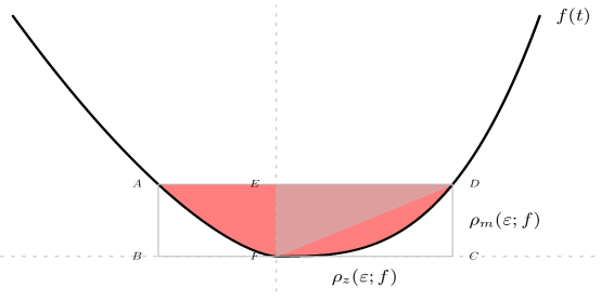
Figure 1: Water filling process.

The geometric quantities $\rho_{m}(\varepsilon;f)$ and $\rho_{z}(\varepsilon;f)$ defined in (2.7) and (2.8) have the following properties.

Proposition 2.1.

For $0<c<1$, $f\in{\mathcal{F}}$,

$$c\leq{\rho_{m}(c\varepsilon;f)\over\rho_{m}(\varepsilon;f)}\leq c^{\frac{2}{3}}\quad\text{and}\quad\max\left\{\left({c\over 2}\right)^{\frac{2}{3}},c\right\}\leq{\rho_{z}(c\varepsilon;f)\over\rho_{z}(\varepsilon;f)}\leq 1.$$ (2.9)

The following result connects the local moduli of continuity to these two geometric quantities.

Proposition 2.2.

Let $\rho_{m}(\varepsilon;f)$ and $\rho_{z}(\varepsilon;f)$ be defined in (2.7) and (2.8), respectively. Then

$$\rho_{m}(\varepsilon;f)\leq\omega_{m}(\varepsilon;f)\leq 3\rho_{m}(\varepsilon;f),$$ (2.10)

$$\rho_{z}(\varepsilon;f)\leq\omega_{z}(\varepsilon;f)\leq 3\rho_{z}(\varepsilon;f).$$ (2.11)

Therefore, through the local moduli of continuity, the hardness of the estimation and inference tasks are tied to the geometry of the convex function near its minimizer. Note that as the function gets flatter near its minimizer, $\rho_{m}(\varepsilon;f)$ decreases while $\rho_{z}(\varepsilon;f)$ increases. It is useful to calculate $\rho_{m}(\varepsilon;f)$ and $\rho_{z}(\varepsilon;f)$ in a concrete example.

Example 2.1.

Consider the function $f(t)=|t-\frac{1}{2}|^{k}$ where $k\geq 1$ is a constant. We will calculate $\rho_{m}(\varepsilon;f)$ and then obtain $\rho_{z}(\varepsilon;f)$ by first computing $\|f-f_{u}\|_{2}^{2}$ and then setting it to $\varepsilon^{2}$ to solve for $\rho_{m}(\varepsilon;f)$.

It is easy to see that in this case $\|f-f_{u}\|_{2}^{2}=\frac{4k^{2}}{(2k+1)(k+1)}\cdot u^{\frac{2k+1}{k}}.$ Setting $\|f-f_{u}\|_{2}^{2}=\varepsilon^{2}$ yields $u=\left(\frac{(2k+1)(k+1)}{4k^{2}}\right)^{\frac{k}{2k+1}}\varepsilon^{\frac{2k}{2k+1}}.$ Hence,

$$\rho_{m}(\varepsilon;f)=\left(\frac{(2k+1)(k+1)}{4k^{2}}\right)^{\frac{k}{2k+1}}\varepsilon^{\frac{2k}{2k+1}}.$$

To compute $\rho_{z}(\varepsilon;f)$, note that $f^{-1}(u)=\frac{1}{2}\pm u^{1\over k}=\frac{1}{2}\pm\left(\frac{(2k+1)(k+1)}{4k^{2}}\right)^{\frac{1}{2k+1}}\varepsilon^{\frac{2}{2k+1}}.$ Hence

$$\rho_{z}(\varepsilon;f)=\min\left\{\left(\frac{(2k+1)(k+1)}{4k^{2}}\right)^{\frac{1}{2k+1}}\varepsilon^{\frac{2}{2k+1}},\frac{1}{2}\right\}.$$

Proposition 2.2 then yields tight bounds for the local moduli of continuity $\omega_{m}(\varepsilon;f)$ and $\omega_{z}(\varepsilon;f)$.

Remark 2.1.

Note that the results obtained in Example 2.1 can be extended to a class of convex functions. For $f\in{\mathcal{F}}$ satisfying

$$0<\varliminf\limits_{t\to{\color[rgb]{0,0,0}Z(f)}}\frac{f(t)-{\color[rgb]{0,0,0}M(f)}}{|t-{\color[rgb]{0,0,0}Z(f)}|^{k}}\leq\varlimsup\limits_{t\to{\color[rgb]{0,0,0}Z(f)}}\frac{f(t)-{\color[rgb]{0,0,0}M(f)}}{|t-{\color[rgb]{0,0,0}Z(f)}|^{k}}<\infty$$

for some $k\geq 1$, it is easy to show that

$$\omega_{m}(\varepsilon;f)\sim\varepsilon^{\frac{2k}{2k+1}},\quad\omega_{z}(\varepsilon;f)\sim\varepsilon^{\frac{2}{2k+1}},\text{ as }\varepsilon\to 0^{+}.$$

2.2 Uncertainty Principle

Section 2.1 provides a precise characterization of the four benchmarks under the non-asymptotic local minimax framework in terms of the local moduli of continuity and the geometric quantities $\rho_{m}(\varepsilon;f)$ and $\rho_{z}(\varepsilon;f)$. These results yield a novel Uncertainty Principle.

Theorem 2.2 (Uncertainty Principle).

Let $R_{z}(\varepsilon;f)$, $R_{m}(\varepsilon;f)$, $L_{z,\alpha}(\varepsilon;f)$, and $L_{m,\alpha}(\varepsilon;f)$ be defined as in (1.2)–(1.7). Let $0<\alpha<0.3$. Then for any $f\in{\mathcal{F}}$,

$$274\varepsilon^{2}>R_{z}(\varepsilon;f)\cdot R_{m}(\varepsilon;f)^{2} \geq \frac{\Phi(-0.5)^{3}}{2}\varepsilon^{2},$$ (2.12)

$$3^{7}\cdot(1-2\alpha)^{3}\varepsilon^{2}>L_{z,\alpha}(\varepsilon;f)\cdot L_{m,\alpha}(\varepsilon;f)^{2} \geq \frac{(0.6-2\alpha)^{3}}{18}\varepsilon^{2}.$$ (2.13)

Note that the bounds in (2.12) and (2.13) are universal for all $f\in{\mathcal{F}}$ and show that there is a fundamental limit to the accuracy of estimation and inference for the minimizer and minimum of a convex function. Our finding here states that the minimizer and the minimum of a convex function cannot be estimated accurately at the same time. This statistical uncertainty principle comes from an intrinsic relationship between the two operators $Z(\cdot)$ and $M(\cdot)$: For any convex function $f\in{\mathcal{F}}$ and any $r>0$, there exists $g\in\partial{\mathcal{B}_{r}}(f)\cap{\mathcal{F}}$ such that

$$|Z(g)-Z(f)|\cdot|M(g)-M(f)|^{2}\geq\frac{1}{2}\left({r\over\varepsilon}\right)^{2}\cdot\varepsilon^{2},$$ (2.14)

where $r/\varepsilon=\|(f-g)/\varepsilon\|_{2}$ characterizes the probabilistic distance between the two convex functions $f$ and $g$ under the white noise model.

Remark 2.2.

To the best of our knowledge, the uncertainty principles established in this paper are the first of their kind in nonparametric statistics in that they reveal the fundamental tensions between estimation/inference of different quantities. It is shown in the Supplementary Material (Cai et al.,, 2021, Section LABEL:subsec:more_on_uncertainty) that similar uncertainty principles also hold for certain subclasses of convex functions. Note that it is not possible to establish such results using conventional minimax analysis where the performance is measured in a worst-case sense over a large parameter space.

2.3 Penalty for Super-efficiency

We have shown that the estimation benchmarks $R_{z}(\varepsilon;f)$ and $R_{m}(\varepsilon;f)$ defined in (1.2) and (1.3) can be characterized by the local moduli of continuity. Before we show in Section 3 that these benchmarks are indeed achievable by adaptive procedures, we first prove that they cannot be essentially outperformed by any estimator uniformly over ${\mathcal{F}}$. The benchmarks $R_{z}(\varepsilon;f)$ and $R_{m}(\varepsilon;f)$ play a role analogous to the information lower bound in classical statistics.

Theorem 2.3 (Penalty for super-efficiency).

For any estimator $\hat{Z}$, if $\mathbb{E}_{f_{0}}|\hat{Z}-Z(f_{0})|\leq\gamma R_{z}(\varepsilon;f_{0})$ for some $f_{0}\in{\mathcal{F}}$ and $\gamma<0.1$, then there exists $f_{1}\in{\mathcal{F}}$ such that

$$\mathbb{E}_{f_{1}}(|\hat{Z}-Z(f_{1})|)\geq\frac{1}{40}\left(\log{1\over\gamma}\right)^{1/3}R_{z}(\varepsilon;f_{1}).$$ (2.15)

Similarly, for any estimator $\hat{M}$, if $\mathbb{E}_{f_{0}}|\hat{M}-M(f_{0})|\leq\gamma R_{m}(\varepsilon;f_{0})$ for some $f_{0}\in{\mathcal{F}}$ and $\gamma<0.1$, then there exists $f_{1}\in{\mathcal{F}}$ such that

$$\mathbb{E}_{f_{1}}|\hat{M}-M(f_{1})|\geq\frac{1}{8}\left(\log{1\over\gamma}\right)^{1/3}R_{m}(\varepsilon;f_{1}).$$ (2.16)

Remark 2.3.

Theorem 2.3 shows that if an estimator of $Z(f)$ or $M(f)$ is super-efficient at some $f_{0}\in{\mathcal{F}}$ in the sense of outperforming the benchmark by a factor of $\gamma$ for some small $\gamma>0$, then it must be sub-efficient at some $f_{1}\in{\mathcal{F}}$ by underperforming the benchmark by at least a factor of $\left(\log{1\over\gamma}\right)^{\frac{1}{3}}$.

3 Adaptive Procedures and Optimality

We now turn to the construction of data-driven and computationally efficient algorithms for estimation and confidence intervals for the minimizer ${\color[rgb]{0,0,0}Z(f)}$ and minimum ${\color[rgb]{0,0,0}M(f)}$ under the white noise model. The procedures are shown to be adaptive to each individual function $f\in{\mathcal{F}}$ in the sense that they simultaneously achieve, up to a universal constant, the corresponding benchmarks $R_{z}(\varepsilon;f)$, $R_{m}(\varepsilon;f)$, $L_{z,\alpha}(\varepsilon;f)$, and $L_{m,\alpha}(\varepsilon;f)$ for all $f\in{\mathcal{F}}$. These results are much stronger than what can be obtained from a conventional minimax analysis.

3.1 The Construction

There are three main building blocks in the construction of the estimators and confidence intervals: Localization, stopping, and estimation/inference.

In the localization step, we begin with the full interval $[0,1]$. Then, iteratively, we halve the intervals and select one halved interval among a set of halved intervals depending on the interval selected in the previous iteration. This set of halved intervals include the two resulting sub-intervals of the previously selected interval and one neighboring halved interval, when such an interval exists, on both sides. The selection rule is to choose the one with the smallest integral of the white noise process over it. See Figure 2 for an illustration of the localization step.

Figure 2: Illustration of the localization step. At level $j$, the middle two intervals are the two subintervals of the selected interval at level $j-1$. One adjacent interval of the same length on each side is added and the interval at level $j$ is selected among these four intervals.

The second step of the construction is the stopping rule. The localization step is iterative, so one needs to determine when there is no further gain and stop the iteration. The integral over each selected interval is a random variable and can be viewed as an estimate of the minimum times the length of the interval. The intuition is that, as the iteration progresses, the bias decreases and the variance increases. As shown in Figure 3, the basic idea is to use the differences of the integrals over the two neighboring intervals 5 blocks away from the current designated interval, when such intervals exist, on both sides. If either of the differences is smaller than 2 standard deviations, then the iteration stops.

Figure 3: Illustration of the stopping rule.

After selecting the final subinterval, the last step in the construction is the estimation/inference for both the minimum and minimizer, which will be described separately later. The detailed construction is given as follows.

3.1.1 Sample Splitting

For technical reasons, we split the data into three independent pieces to ensure independence of the data used in the three steps of the construction. This is done as follows.

Let $B_{1}(t)$ and $B_{2}(t)$ be two independent standard Brownian motions, and both be independent of the observed data $Y$. Let

$$\begin{split}Y_{l}(t)&=Y(t)+\frac{\sqrt{2}}{2}\varepsilon B_{1}(t)+\frac{\sqrt{6}}{2}\varepsilon B_{2}(t),\\ Y_{s}(t)&=Y(t)+\frac{\sqrt{2}}{2}\varepsilon B_{1}(t)-\frac{\sqrt{6}}{2}\varepsilon B_{2}(t),\\ Y_{e}(t)&=Y(t)-\sqrt{2}\varepsilon B_{1}(t),\end{split}$$ (3.1)

for $t\in[0,1]$.

Then $Y_{l}(\cdot)$, $Y_{s}(\cdot)$ and $Y_{e}(\cdot)$ are independent and can be written as

$$\begin{split}dY_{l}(t)&=f(t)dt+\sqrt{3}\varepsilon dW_{1}(t),\\ dY_{s}(t)&=f(t)dt+\sqrt{3}\varepsilon dW_{2}(t),\\ dY_{e}(t)&=f(t)dt+\sqrt{3}\varepsilon dW_{3}(t),\end{split}$$ (3.2)

where $W_{1}$, $W_{2}$ and $W_{3}$ are independent standard Brownian motions.

We now have three independent copies: $Y_{l}$ is used for localization, $Y_{s}$ for stopping, and $Y_{e}$ for the construction of the final estimator and confidence interval for the minimum.

Remark 3.1.

If one is only interested in estimation and inference for the minimizer, the copy $Y_{e}$ is not needed, and it suffices to split into two independent copies with smaller variance. This leads to slightly better performance. Another point is that, although here the three processes $Y_{l}$, $Y_{s}$, and $Y_{e}$ are made to have the same noise level, it is not necessary for the noise levels to be the same. For the simplicity and ease of presentation, we split the original sample into three independent and homoskedastic copies for estimation and inference for both the minimizer and minimum.

3.1.2 Localization

For $j=0,1,\dots$, and $i=0,1,\dots,2^{j}$, let

$$m_{j}=2^{-j},\;t_{j,i}=i\cdot m_{j},\;\text{and}\;\,i^{*}_{j}=\max\{i:Z(f)\in[t_{j,i-1},t_{j,i}]\}.$$ (3.3)

That is, at level $j$ for $j=0,1,\dots$, the $i^{*}_{j}$-th subinterval is the one containing the minimizer $Z(f)$. For $j=0,1,\dots,$ and $i=1,2,\dots,2^{j}$, define

$$X_{j,i}=\int_{t_{j,i-1}}^{t_{j,i}}\mathrm{d}Y_{l}(t),$$

where $Y_{l}$ is one of the three independent copies constructed above through sample splitting. For convenience, we define $X_{j,i}=+\infty$ for $j=0,1,\dots,$ and $i\in\mathbb{Z}\setminus\{1,2,\dots,2^{j}\}$.

Let $\hat{i}_{0}=1$ and for $j=1,2,\dots$, let

$$\hat{i}_{j}=\operatorname*{\arg\min}_{2\hat{i}_{j-1}-2\leq i\leq 2\hat{i}_{j-1}+1}X_{j,i}.$$

Note that given the value of $\hat{i}_{j-1}$ at level $j-1$, in the next iteration the procedure halves the interval $[t_{\hat{i}_{j-1}-1},t_{\hat{i}_{j-1}}]$ into two subintervals and selects the interval $[t_{\hat{i}_{j}-1},t_{\hat{i}_{j}}]$ at level $j$ from these and their immediate neighboring subintervals. So $i$ only ranges over 4 possible values at level $j$. See Figure 2 for an illustration.

3.1.3 Stopping Rule

It is necessary to have a stopping rule to select a final subinterval constructed in the localization iterations. We use another independent copy $Y_{s}$ constructed in the sample splitting step to devise a stopping rule. For $j=0,1,\dots,$ and $i=1,2,\dots,2^{j}$, let

$$\tilde{X}_{j,i}=\int_{t_{j,i-1}}^{t_{j,i}}\mathrm{d}Y_{s}(t).$$

Again, for convenience, we define $\tilde{X}_{j,i}=+\infty$ for $j=0,1,\dots,$ and $i\in\mathbb{Z}\setminus\{1,2,\dots,2^{j}\}$. Let the statistic $T_{j}$ be defined as

$$T_{j}=\min\{\tilde{X}_{j,\hat{i}_{j}+6}-\tilde{X}_{j,\hat{i}_{j}+5},\;\tilde{X}_{j,\hat{i}_{j}-6}-\tilde{X}_{j,\hat{i}_{j}-5}\},$$

where we use the convention $+\infty-x=+\infty$ and $\min\{+\infty,x\}=x$, for any $-\infty\leq x\leq\infty$.

The stopping rule is based on the value of $T_{j}$. It is helpful to provide some intuition before formally defining the stopping rule. Intuitively, the algorithm should stop at a place where the signal to noise ratio of $T_{j}$ is small or where the signal is negative. Let $\sigma_{j}^{2}=6m_{j}\varepsilon^{2}$. It is easy to see that, when $\tilde{X}_{j,\hat{i}_{j}+6}-\tilde{X}_{j,\hat{i}_{j}+5}<\infty$,

$$\tilde{X}_{j,\hat{i}_{j}+6}-\tilde{X}_{j,\hat{i}_{j}+5}\big{|}\hat{i}_{j}\sim N\left(\int_{t_{j,\hat{i}_{j}+5}}^{t_{j,\hat{i}_{j}+6}}\left(f(t+m_{j})-f(t)\right)dt,\;\sigma_{j}^{2}\right).$$ (3.4)

Note that the standard deviation $\sigma_{j}$ decreases at the rate $\frac{1}{\sqrt{2}}$ as $j$ increases. We now turn to the mean of $\tilde{X}_{j,\hat{i}_{j}+6}-\tilde{X}_{j,\hat{i}_{j}+5}|\hat{i}_{j}$. Recall the notation introduced in (3.3). It is easy to see that the algorithm should stop as soon as $\int_{t_{j,\hat{i}_{j}+5}}^{t_{j,\hat{i}_{j}+6}}\left(f(t+m_{j})-f(t)\right)dt$ turns negative, since for any $\hat{i}_{j}$, if $\int_{t_{j,\hat{i}_{j}+5}}^{t_{j,\hat{i}_{j}+6}}\left(f(t+m_{j})-f(t)\right)dt<0$, then $|\hat{i}_{j}-i^{*}_{j}|\geq 5$ and consequently $|\hat{i}_{j_{1}}-i^{*}_{j_{1}}|\geq 5$ for any $j_{1}\geq j$. When $\int_{t_{j,\hat{i}_{j}+5}}^{t_{j,\hat{i}_{j}+6}}\left(f(t+m_{j})-f(t)\right)dt$ is positive, a careful analysis in the proof shows that it shrinks at a rate faster than or equal to ${1\over 4}$ as $j$ increases. Analogous results hold for $\tilde{X}_{j,\hat{i}_{j}-6}-\tilde{X}_{j,\hat{i}_{j}-5}\big{|}\hat{i}_{j}$.

Finally, the iterations stop at level $\hat{j}$ where

$$\hat{j}=\min\{j:\frac{T_{j}}{\sigma_{j}}\leq 2\}.$$

The subinterval containing the minimizer $Z(f)$ is localized to be $[t_{\hat{j},\hat{i}_{\hat{j}}-1},t_{\hat{j},\hat{i}_{\hat{j}}}]$.

3.1.4 Estimation and Inference

After the final subinterval $[t_{\hat{j},\hat{i}_{\hat{j}}-1},t_{\hat{j},\hat{i}_{\hat{j}}}]$ is obtained, we then use it to construct estimators and confidence intervals for $Z(f)$ and$M(f)$. We begin with the minimizer $Z(f)$. The estimator of $Z(f)$ is given by the midpoint of the interval $[t_{\hat{j},\hat{i}_{\hat{j}}-1},t_{\hat{j},\hat{i}_{\hat{j}}}]$, i.e.,

$$\hat{Z}=\frac{t_{\hat{j},\hat{i}_{\hat{j}}}+t_{\hat{j},\hat{i}_{\hat{j}}-1}}{2}.$$ (3.5)

To construct the confidence interval for ${\color[rgb]{0,0,0}Z(f)}$, one needs to take a few steps to the left and to the right at level $\hat{j}$. Let $K_{\alpha}=\lceil\frac{\log{\alpha}}{\log{\Phi(-2)}}\rceil$ and define

$$L=\max\{0,\;\hat{i}_{\hat{j}}-12\times 2^{K_{\alpha}}+1\},\quad U=\min\{2^{\hat{j}},\;\hat{i}_{\hat{j}}+12\times 2^{K_{\alpha}}-2\}.$$

The $1-\alpha$ confidence interval for $Z(f)$ is given by

$$CI_{z,\alpha}=[t_{\hat{j},L},\;t_{\hat{j},U}].$$ (3.6)

For estimation of and confidence interval for the minimum $M(f)$, define

$$\bar{X}_{j,i}=\int_{t_{j,i-1}}^{t_{j,i}}Y_{e}(t)dt.$$

Let ${\tilde{i}}_{\hat{j}}=\hat{i}_{\hat{j}}+2\left(\mathbbm{1}\{\tilde{X}_{\hat{j},\hat{i}_{\hat{j}}+6}-\tilde{X}_{j,\hat{i}_{\hat{j}}+5}\leq 2\sigma_{\hat{j}}\}-\mathbbm{1}\{\tilde{X}_{\hat{j},\hat{i}_{\hat{j}}-6}-\tilde{X}_{j,\hat{i}_{\hat{j}}-5}\leq 2\sigma_{\hat{j}}\}\right)$ and define the final estimator of the minimum $M(f)$ by

$$\hat{M}=\frac{1}{m_{\hat{j}}}\bar{X}_{\hat{j},{\tilde{i}}_{\hat{j}}}.$$ (3.7)

We now construct confidence interval for ${\color[rgb]{0,0,0}M(f)}$. Recall that $K_{\alpha}=\lceil\frac{\log{\alpha}}{\log{\Phi(-2)}}\rceil$. Compared with the confidence interval for the minimizer, we take four more blocks on each side at the level $(\hat{j}-K_{\frac{\alpha}{4}}-1)_{+}$. More specifically, we define

$$t_{L}=t_{(\hat{j}-K_{\frac{\alpha}{4}}-1)_{+},\hat{i}_{(\hat{j}-K_{\frac{\alpha}{4}}-1)_{+}}-5},\quad t_{R}=t_{(\hat{j}-K_{\frac{\alpha}{4}}-1)_{+},\hat{i}_{(\hat{j}-K_{\frac{\alpha}{4}}-1)_{+}}+4}.$$

Set

$$\tilde{K}_{\alpha}=\max\{4,\;2+\lceil\log_{2}{(2+z_{\alpha/3})}\rceil\}.$$ (3.8)

Note that at level $\hat{j}+\tilde{K}_{\frac{\alpha}{4}}$, the indices of the intervals with right endpoints $t_{L}$, $t_{R}$ respectively are

$$i_{L}=t_{L}\cdot 2^{\hat{j}+\tilde{K}_{\frac{\alpha}{4}}}\quad\text{and}\quad i_{R}=t_{R}\cdot 2^{\hat{j}+\tilde{K}_{\frac{\alpha}{4}}}.$$

Note also that $i_{R}-i_{L}=9\times 2^{1+\tilde{K}_{\frac{\alpha}{4}}+K_{\frac{\alpha}{4}}}$, which only depends on $\alpha$. Define an intermediate estimator of the minimum $M(f)$ by

$$\hat{f}_{1}=\frac{1}{m_{\hat{j}+\tilde{K}_{\frac{\alpha}{4}}}}\min_{i_{L}<i\leq i_{R}}\bar{X}_{\hat{j}+\tilde{K}_{\frac{\alpha}{4}},i}.$$

Let $F_{n}$ be the cumulative distribution function of $\tilde{v}_{n}=\max\{v_{1},\dots,v_{n}\}$, where $v_{1},\dots,v_{n}\overset{i.i.d}{\sim}N(0,1)$, and define

$$S_{n,\beta}=F_{n}^{-1}(1-\beta).$$ (3.9)

In other words, $S_{n,\beta}$ is the $(1-\beta)$ quantile of the distribution of the maximum of n $i.i.d.$ standard normal variables. Let

$$f_{lo}=\hat{f}_{1}-z_{\alpha/4}\frac{\sqrt{3}\varepsilon}{\sqrt{m_{\hat{j}+\tilde{K}_{\frac{\alpha}{4}}}}}-\frac{\sqrt{3}\varepsilon}{\sqrt{m_{\hat{j}+\tilde{K}_{\frac{\alpha}{4}}}}},\quad f_{hi}=\hat{f}_{1}+S_{i_{R}-i_{L},\frac{\alpha}{4}}\cdot\frac{\sqrt{3}\varepsilon}{\sqrt{m_{\hat{j}+\tilde{K}_{\frac{\alpha}{4}}}}}.$$

Then the $(1-\alpha)$ level confidence interval for $M(f)$ is defined as

$$CI_{m,\alpha}=[f_{lo},\;f_{hi}].$$ (3.10)

3.2 Statistical Optimality

Now we establish the optimality of the adaptive procedures constructed in Section 3.1. The results show that the data-driven estimators and the confidence intervals attain their corresponding local minimax risks/lengths in the sense of staying within a constant multiplier. We begin with the estimator of the minimizer.

Theorem 3.1 (Estimation of Minimizer).

The estimator $\hat{Z}$ defined in (3.5) satisfies

$$\mathbb{E}_{f}|\hat{Z}-{\color[rgb]{0,0,0}Z(f)}|<35\rho_{z}(\varepsilon;f)\leq C_{z}R_{z}(\varepsilon;f),\quad\text{for all $f\in{\mathcal{F}}$},$$

where $C_{z}>0$ is an absolute constant.

The following result holds for the confidence interval $CI_{z,\alpha}$.

Theorem 3.2 (Confidence Interval for the Minimizer).

Let $0<\alpha<0.3$. The confidence interval $CI_{z,\alpha}$ given in (3.6) is a $(1-\alpha)$ level confidence interval for the minimizer $Z(f)$ and its expected length satisfies

$$\mathbb{E}_{f}L(CI_{z,\alpha})\leq(24\times 2^{K_{\alpha}}-3)\times 17.5\times\rho_{z}(\varepsilon;f)\leq C_{z,\alpha}L_{z,\alpha}(\varepsilon;f),\quad\text{for all $f\in{\mathcal{F}}$},$$

where $K_{\alpha}=\lceil\frac{\log{\alpha}}{\log{\Phi(-2)}}\rceil$ and $C_{z,\alpha}$ is a constant depending on $\alpha$ only.

Similarly, the estimator and confidence interval for the minimum $M(f)$ are within a constant factor of the benchmarks simultaneously for all $f\in{\mathcal{F}}$.

Theorem 3.3 (Estimation of Minimum).

The estimator $\hat{M}$ defined in (3.7) satisfies

$$\mathbb{E}_{f}|{\color[rgb]{0,0,0}\hat{M}-M(f)}|<449\rho_{m}(\varepsilon;f)\leq C_{m}R_{m}(\varepsilon;f),\quad\text{for all $f\in{\mathcal{F}}$},$$

where $C_{m}>0$ is an absolute constant.

Theorem 3.4 (Confidence Interval for the Minimum).

The confidence interval $CI_{m,\alpha}$ given in (3.10) is a $(1-\alpha)$ confidence interval for the minimum $M(f)$ and when $0<\alpha<0.3$, its expected length satisfies

$$\mathbb{E}_{f}L(CI_{m,\alpha})\leq c_{m,\alpha}\rho_{m}(\varepsilon;f)\leq C_{m,\alpha}L_{m,\alpha}(\varepsilon;f),\quad\text{for all $f\in{\mathcal{F}}$},$$

where $c_{m,\alpha}$ and $C_{m,\alpha}$ are constants depending on $\alpha$ only.

4 Nonparametric Regression

We have so far focused on the white noise model. The procedures and results presented in the previous sections can be extended to nonparametric regression, where we observe

$$y_{i}=f(x_{i})+\sigma z_{i},\quad i=0,1,2,\ldots,n,$$ (4.1)

with $x_{i}=\frac{i}{n}$, and $z_{i}\overset{i.i.d}{\sim}N(0,1).$ The noise level $\sigma$ is assumed to be known. The tasks are the same as before: construct optimal estimators and confidence intervals for the minimizer and minimum of $f\in{\mathcal{F}}$.

4.1 Benchmarks and Discretization Errors

Analogous to the benchmarks for the white noise model defined in Equations (1.2), (1.3), (1.6), (1.7), we define similar benchmarks for the nonparametric regression model (4.1) with $n+1$ equally spaced observations. Denote by $\mathcal{I}_{z,\alpha,n}(\mathfrak{F})$ and $\mathcal{I}_{m,\alpha,n}(\mathfrak{F})$ respectively the collections of $(1-\alpha)$ level confidence intervals for $Z(f)$ and $M(f)$ on a function class $\mathfrak{F}$ under the regression model (4.1) and let

$$\begin{split}\tilde{R}_{z,n}(\sigma;f)=&\sup_{g\in{\mathcal{F}}}\inf_{\hat{Z}}\max_{h\in\{f,g\}}\mathbb{E}_{h}|\hat{Z}-Z(h)|,\\ \tilde{R}_{m,n}(\sigma;f)=&\sup_{g\in{\mathcal{F}}}\inf_{\hat{M}}\max_{h\in\{f,g\}}\mathbb{E}_{h}|\hat{M}-M(h)|,\\ \tilde{L}_{z,\alpha,n}(\sigma;f)=&\sup_{g\in{\mathcal{F}}}\inf_{CI\in\mathcal{I}_{z,\alpha,n}(\{f,g\})}\mathbb{E}_{f}L(CI),\\ \tilde{L}_{m,\alpha,n}(\sigma;f)=&\sup_{g\in{\mathcal{F}}}\inf_{CI\in\mathcal{I}_{m,\alpha,n}(\{f,g\})}\mathbb{E}_{f}L(CI).\end{split}$$ (4.2)

Compared with the white noise model, estimation and inference for both $Z(f)$ and $M(f)$ incur additional discretization errors, even in the noiseless case. See the Supplementary Material (Cai et al.,, 2021, Section LABEL:sec:nonparametric_benchmarks_lowerbounds) for further discussion.

4.2 Data-driven Procedures

Similar to the white noise model, we first split the data into three independent copies and then construct the estimators and confidence intervals for $Z(f)$ and $M(f)$ in three major steps: localization, stopping, and estimation/inference.

4.2.1 Data Splitting

Let $z_{1,0},z_{1,1},\ldots,z_{1,n},z_{2,0},z_{2,1},\ldots,z_{2,n}$ be i.i.d. standard normal random variables, and all be independent of the observed data $\{y_{1},...,y_{n}\}$. We construct the following three sequences:

$$\begin{split}&y_{l,i}=y_{i}+\frac{\sqrt{2}}{2}\sigma z_{1,i}+\frac{\sqrt{6}}{2}\sigma z_{2,i},\\ &y_{s,i}=y_{i}+\frac{\sqrt{2}}{2}\sigma z_{1,i}-\frac{\sqrt{6}}{2}\sigma z_{2,i},\\ &y_{e,i}=y_{i}-\sqrt{2}\sigma z_{1,i},\end{split}$$ (4.3)

for $i=0,\ldots,n$. For convenience, let $y_{l,i}=y_{s,i}=y_{e,i}=\infty$ for $i\not\in\{0,1,\ldots,n\}$. It is easy to see that these random variables are all independent with the same variance $3\sigma^{2}$ for $i\in\{0,1,\ldots,n\}$. We will use $\{y_{l,i}\}$ for localization, $\{y_{s,i}\}$ for devising the stopping rule, and $\{y_{e,i}\}$ for constructing the final estimation and inference procedures.

Let $J=\lfloor\log_{2}(n+1)\rfloor$. For $j=0,1,\ldots,J$, $i=1,2,\ldots,\lfloor\frac{n+1}{2^{J-j-1}}\rfloor$, the $i$-th block at level $j$ consists of $\{x_{(i-1)2^{J-j}},x_{(i-1)2^{J-j}+1},\ldots,x_{i\cdot 2^{J-j}-1}\}$. Denote the sum of the observations in the $i$-th block at level $j$ for the sequence $u$ ($u=l,s,e$) as

$$Y_{j,i,u}=\sum_{k=(i-1)2^{J-j}}^{i\cdot 2^{J-j}-1}y_{u,k},\text{ for }u=l,s,e.$$

Again, let $Y_{j,i,u}=+\infty$ when $i\in\mathbbm{Z}\backslash\{1,2,\ldots,\lfloor\frac{n+1}{2^{J-j-1}}\rfloor\}$, for $u=l,s,e$.

4.2.2 Localization

We now use $\{y_{l,i},i=0,\ldots,n\}$ to construct a localization procedure. Let $\mathtt{\hat{i}}_{0}=1$, and for $j=1,2,\ldots,J$, let

$$\mathtt{\hat{i}}_{j}=\operatorname*{\arg\min}_{\max\{2\mathtt{\hat{i}}_{j-1}-2,1\}\leq i\leq\min\{2\mathtt{\hat{i}}_{j-1}+1,\lfloor\frac{n+1}{2^{J-j}}\rfloor\}}Y_{j,i,l}.$$

This is similar to the localization step in the white noise model. In each iteration, the blocks at the previous level are split into two sub-blocks. The $i$-th block at level $j-1$ is split into two blocks, the $(2i-1)$-st block and $2i$-th block, at level $j$. For a given $\mathtt{\hat{i}}_{j-1}$, $\mathtt{\hat{i}}_{j}$ is the sub-block with the smallest sum among the two sub-blocks of $(j-1)$-level-block $\mathtt{\hat{i}}_{j-1}$ and their immediate neighboring sub-blocks.

4.2.3 Stopping Rule

Similar to the stopping rule for the white noise model, define the statistic $\mathtt{T}_{j}$ as

$$\mathtt{T}_{j}=\min\{Y_{j,\mathtt{\hat{i}}_{j}+6,s}-Y_{j,\mathtt{\hat{i}}_{j}+5,s},\;Y_{j,\mathtt{\hat{i}}_{j}-6,s}-Y_{j,\mathtt{\hat{i}}_{j}-5,s}\}.$$

Let $\tilde{\sigma}_{j}^{2}=6\times 2^{J-j}\sigma^{2}$. It is easy to see that when $Y_{j,\mathtt{\hat{i}}_{j}+6,s}-Y_{j,\mathtt{\hat{i}}_{j}+5,s}<\infty$,

$$Y_{j,\mathtt{\hat{i}}_{j}+6,s}-Y_{j,\mathtt{\hat{i}}_{j}+5,s}|\mathtt{\hat{i}}_{j}\sim N(\sum_{k=(\mathtt{\hat{i}}_{j}+4)2^{J-j}}^{(\mathtt{\hat{i}}_{j}+5)2^{J-j}-1}f(x_{k+2^{J-j}})-f(x_{k}),\tilde{\sigma}_{j}^{2}).$$ (4.4)

Define

$${\check{j}}=\left\{\begin{array}[]{ll}\min\{j:\mathtt{T}_{j}\leq 2\tilde{\sigma}_{j}\}&\text{if}\;\{j:\mathtt{T}_{j}\leq 2\tilde{\sigma}_{j}\}\cap\{0,1,2,\ldots,J\}\not=\emptyset\\ \infty&\text{otherwise}\end{array}\right.$$

and terminate the algorithm at level $\mathtt{\hat{j}}=\min\{J,{\check{j}}\}$. So, either $\mathtt{T}_{j}$ triggers the stopping rule for some $0\leq j\leq J$ or the algorithm reaches the highest possible level $J$.

With the localization strategy and the stopping rule, the final block, the $\mathtt{\hat{i}}_{\mathtt{\hat{j}}}$-th block at level $\mathtt{\hat{j}}$, is given by $\{x_{k}:(\mathtt{\hat{i}}_{\mathtt{\hat{j}}}-1)2^{J-\mathtt{\hat{j}}}\leq k\leq\mathtt{\hat{i}}_{\mathtt{\hat{j}}}2^{J-\mathtt{\hat{j}}}-1\}$.

4.2.4 Estimation and Inference

After we have our final block, $\mathtt{\hat{i}}_{\mathtt{\hat{j}}}$-th block at level $\mathtt{\hat{j}}$, we use it to construct estimators and confidence intervals for the minimizer $Z(f)$ and the minimum $M(f)$. We start with the estimation of $Z(f)$. The estimator of $Z(f)$ is given as follows:

$$\hat{Z}=\left\{\begin{aligned} -\frac{1}{2n}+\frac{1}{n}(2^{J-\mathtt{\hat{j}}}\mathtt{\hat{i}}_{\mathtt{\hat{j}}}-2^{J-\mathtt{\hat{j}}-1}),&\qquad\check{j}<\infty\\ \frac{1}{n}\arg\min_{\mathtt{\hat{i}}_{\mathtt{\hat{j}}}-2\leq i\leq\mathtt{\hat{i}}_{\mathtt{\hat{j}}}+2}y_{e,i-1}-{1\over n},&\qquad\check{j}=\infty\end{aligned}\right.$$ (4.5)

To construct the confidence interval for $Z(f)$, we take a few adjacent blocks to the left and right of $\mathtt{\hat{i}}_{\mathtt{\hat{j}}}$-th block at level $\mathtt{\hat{j}}$. Let

$$\mathtt{L}=\max\{0,\mathtt{\hat{i}}_{\mathtt{\hat{j}}}-12\times 2^{K_{\alpha/2}}+1\}\quad\text{\rm and}\quad\mathtt{U}=\min\{\lceil(n+1)2^{\mathtt{\hat{j}}-J}\rceil,\mathtt{\hat{i}}_{\mathtt{\hat{j}}}+12\times 2^{K_{\alpha/2}}-2\}.$$

When $\check{j}<\infty$, let

$$t_{lo}=\frac{2^{J-\mathtt{\hat{j}}}}{n}\mathtt{L}-\frac{1}{2n}\quad\text{\rm and}\quad t_{hi}=\frac{2^{J-\mathtt{\hat{j}}}}{n}\mathtt{U}-\frac{1}{2n}.$$

When $\check{j}=\infty$, $t_{lo}$ and $t_{hi}$ are calculated by the following Algorithm 1. Note that $\check{j}=\infty$ means that the procedure is forced to end and the discretization error can be dominant.

Algorithm 1 first iteratively shrinks the original interval $[t_{lo}-{1\over n},t_{hi}+{1\over n}]$ to find the minimizer ${i_{m}\over n}$ of the function $f$ among the $n+1$ sample points with high probability. In each iteration, the algorithm tests whether the slopes of the segments on both ends are positive or negative. It shrinks the left end with negative slope (on the left), or shrinks the right end with positive slope (on the right), or stops if no further shrinking is needed on either side.

Note that the minimizer of any convex function with given values at these $n+1$ points is smaller than the intersection of the following two lines:

$$y=f({i_{m}\over n})\quad\text{and}\quad y={f({i_{m}+2\over n})-f({i_{m}+1\over n})\over 1/n}(t-{i_{m}+1\over n})+f({i_{m}+1\over n}).$$ (4.6)

Note that these two lines are determined by $f({i_{m}\over n})$, $f({i_{m}+1\over n})$ and $f({i_{m}+2\over n})$ only. Given the noisy observations at these three points, ${i_{m}\over n}$, ${i_{m}+1\over n}$, and ${i_{m}+2\over n}$, the range of these two lines and the intersection can be inferred, and the right side of the interval can then be shrunk accordingly.

Similar is done for the left side of the confidence interval. In addition, boundary cases and other complications need to be considered, which are handled in Algorithm 1.

Note that our construction and the theoretical results only rely on convexity. In particular, the existence of second order derivative is not needed as it is commonly assumed in the literature. This is an important contributing factor to optimality under the non-asymptotic local minimax framework.

Algorithm 1 Computing $t_{lo}$ and $t_{hi}$ when $\check{j}=\infty$

  $L\leftarrow\max\{1,\mathtt{\hat{i}}_{\mathtt{\hat{j}}}-12\times 2^{K_{\alpha/2}}\}-1$ , $U\leftarrow\min\{n+1,\mathtt{\hat{i}}_{\mathtt{\hat{j}}}+12\times 2^{K_{\alpha/2}}\}-1$, $\alpha_{1}\leftarrow\frac{\alpha}{8}$, $\alpha_{2}=\alpha/24$

  Generate $z_{3,0},z_{3,1}\ldots,z_{3,n}\overset{i.i.d.}{\sim}N(0,1)$

  $i_{l}\leftarrow\min\{\{U\}\cup\{i\in[L,U-1]:y_{e,i}+\sqrt{3}\sigma z_{3,i}-(y_{e,i+1}+\sqrt{3}\sigma z_{3,i+1})\leq 2\sqrt{3}\sigma z_{\alpha_{1}}\}\}$ $i_{r}\leftarrow\max\{\{L-1\}\cup\{i\in[L,U-1]:y_{e,i}+\sqrt{3}\sigma z_{3,i}-(y_{e,i+1}+\sqrt{3}\sigma z_{3,i+1})\geq-2\sqrt{3}\sigma z_{\alpha_{1}}\}\}$

  if $i_{l}=U$ then

     if $i_{l}=n$ and $y_{e,n-2}-y_{e,n-1}-\sqrt{3}\sigma(z_{3,n-2}-z_{3,n-1})+2\sqrt{6}\sigma z_{\alpha_{2}}>0$  then

        

$$t_{lo}\leftarrow\left((-\frac{y_{e,n}-y_{e,n-1}-\sqrt{3}\sigma(z_{3,n}-z_{3,n-1})+2\sqrt{6}\sigma z_{\alpha_{2}}}{n(y_{e,n-2}-y_{e,n-1}-\sqrt{3}\sigma(z_{3,n-2}-z_{3,n-1})+2\sqrt{6}\sigma z_{\alpha_{2}})}+\frac{n-1}{n})\vee\frac{n-1}{n}\right)\wedge\frac{n}{n},$$

$t_{hi}\leftarrow 1$

     else

        $t_{lo}=t_{hi}=U/n$

     end if

  end if

  if $i_{r}=L-1$ then

     if $i_{r}=-1$ and $y_{e,2}-y_{e,1}-\sqrt{3}\sigma(z_{3,2}-z_{3,1})+2\sqrt{6}\sigma z_{\alpha_{2}}>0$  then

        

$$t_{hi}\leftarrow\left((\frac{y_{e,0}-y_{e,1}-\sqrt{3}\sigma(z_{3,0}-z_{3,1})+2\sqrt{6}\sigma z_{\alpha_{2}}}{n(y_{e,2}-y_{e,1}-\sqrt{3}\sigma(z_{3,2}-z_{3,1})+2\sqrt{6}\sigma z_{\alpha_{2}})}+\frac{1}{n})\vee\frac{0}{n}\right)\wedge\frac{1}{n},t_{lo}=0$$

     else

        $t_{lo}=t_{hi}=0$

     end if

  end if

  if $(i_{l}-U)(i_{r}-L+1)\not=0$ then

     $i_{lo}\leftarrow(i_{l}-1)\vee L$, $i_{hi}\leftarrow(i_{r}+2)\wedge U$

     if  $i_{hi}-i_{lo}\geq 3$ or $(i_{hi}-n)i_{lo}=0$  then

        $t_{lo}=i_{lo}/n$, $t_{hi}=i_{hi}/n$

     else if  $y_{e,i_{hi}+1}-y_{e,i_{hi}}-\sqrt{3}\sigma(z_{3,i_{hi}+1}-z_{3,i_{hi}})\leq-2\sqrt{6}\sigma z_{\alpha_{2}}$ or $y_{e,i_{lo}-1}-y_{e,i_{lo}}-\sqrt{3}\sigma(z_{3,i_{lo}-1}-z_{3,i_{lo}})\leq-2\sqrt{6}\sigma z_{\alpha_{2}}$  then

        $t_{lo}=t_{hi}=(i_{hi}+i_{lo})/2n$

     else

        

$$t_{hi}\leftarrow\left((\frac{y_{e,i_{hi}-1}-y_{e,i_{hi}}-\sqrt{3}\sigma(z_{3,i_{hi}-1}-z_{3,i_{hi}})+2\sqrt{6}\sigma z_{\alpha_{2}}}{n(y_{e,i_{hi}+1}-y_{e,i_{hi}}-\sqrt{3}\sigma(z_{3,i_{hi}+1}-z_{3,i_{hi}})+2\sqrt{6}\sigma z_{\alpha_{2}})}+\frac{i_{hi}}{n})\vee\frac{i_{hi}-1}{n}\right)\wedge\frac{i_{hi}}{n}$$

$$t_{lo}\leftarrow\left((-\frac{y_{e,i_{lo}+1}-y_{e,i_{lo}}-\sqrt{3}\sigma(z_{3,i_{lo}+1}-z_{3,i_{lo}})+2\sqrt{6}\sigma z_{\alpha_{2}}}{n(y_{e,i_{lo}-1}-y_{e,i_{lo}}-\sqrt{3}\sigma(z_{3,i_{lo}-1}-z_{3,i_{lo}})+2\sqrt{6}\sigma z_{\alpha_{2}})}+\frac{i_{lo}}{n})\vee\frac{i_{lo}}{n}\right)\wedge\frac{i_{lo}+1}{n}$$

     end if

  end if

The $(1-\alpha)$-level confidence interval for the minimizer $Z(f)$ is given by

$$\mathtt{CI}_{z,\alpha}=[t_{lo}\wedge t_{hi},t_{hi}]$$ (4.7)

We now construct the estimator and confidence interval for the minimum $M(f)$. Let $\Delta=\mathbbm{1}\{Y_{\mathtt{\hat{j}},\mathtt{\hat{i}}_{\mathtt{\hat{j}}}+6,s}-Y_{\mathtt{\hat{j}},\mathtt{\hat{i}}_{\mathtt{\hat{j}}}+5,s}\leq 2\sqrt{6}\sigma\sqrt{2^{J-\mathtt{\hat{j}}}}\}-\mathbbm{1}\{Y_{\mathtt{\hat{j}},\mathtt{\hat{i}}_{\mathtt{\hat{j}}}-6,s}-Y_{\mathtt{\hat{j}},\mathtt{\hat{i}}_{\mathtt{\hat{j}}}-5,s}\leq 2\sqrt{6}\sigma\sqrt{2^{J-\mathtt{\hat{j}}}}\}$ and define

$$\tilde{\mathtt{i}}_{\mathtt{\hat{j}}}=\left\{\begin{array}[]{ll}\mathtt{\hat{i}}_{\mathtt{\hat{j}}}+2\Delta&\quad\text{if ${\check{j}}<\infty$}\\ \operatorname*{\arg\min}_{\mathtt{\hat{i}}_{\mathtt{\hat{j}}}-2\leq i\leq\mathtt{\hat{i}}_{\mathtt{\hat{j}}}+2}y_{e,i-1}&\quad\text{if ${\check{j}}=\infty$}\end{array}\right..$$ (4.8)

The estimator of $M(f)$ is then given by the average of the observations of the copy for estimation and inference in the $\tilde{\mathtt{i}}_{\mathtt{\hat{j}}}$-th block at level $\mathtt{\hat{j}}$,

$$\hat{M}=\frac{1}{2^{J-\mathtt{\hat{j}}}}Y_{\mathtt{\hat{j}},\tilde{\mathtt{i}}_{\mathtt{\hat{j}}},e}.$$ (4.9)

To construct the confidence interval for $M(f)$, we specify two levels $j_{s}$ and $j_{l}$, with

$$j_{s}=\max\{0,\mathtt{\hat{j}}-K_{\frac{\alpha}{4}}-1\}\quad\text{and}\quad j_{l}=\min\{J,\mathtt{\hat{j}}+\tilde{K}_{\frac{\alpha}{4}}\},$$

where $\tilde{K}_{\frac{\alpha}{4}}$ is defined as in Equation (3.8). It will be shown that at level $j_{s}$, $Z(f)$ is within four blocks of the chosen block with probability at least $1-\frac{\alpha}{4}$, and at level $j_{l}$, with probability at least $1-\frac{\alpha}{4}$, the length of the block is no larger than $\rho_{z}(\frac{\sigma}{\sqrt{n}};f)$. Define

$$I_{lo}=\max\{1,2^{j_{l}-j_{s}}(\mathtt{\hat{i}}_{j_{s}}-5)\},\quad I_{hi}=\min\{2^{j_{l}-j_{s}}(\mathtt{\hat{i}}_{j_{s}}+4)+1,\lceil\frac{n+1}{2^{J-j_{l}}}\rceil\}.$$

It can be shown that the minimizer $Z(f)$ lies with high probability in the interval $[\frac{2^{J-j_{l}}(I_{lo}-1)}{n},\frac{2^{J-j_{l}}I_{hi}-1}{n}]\cap[0,1]$. Define an intermediate estimator for $M(f)$ by

$$\mathtt{\hat{f}}_{1}=\min_{I_{lo}\leq i\leq I_{hi}}\frac{1}{2^{J-j_{l}}}Y_{j_{l},i,e}.$$

Let

$$\mathtt{f}_{hi}=\mathtt{\hat{f}}_{1}+S_{I_{hi}-I_{lo}+1,\frac{\alpha}{4}}\frac{\sqrt{3}\sigma}{\sqrt{2^{J-j_{l}}}}$$

where $S_{n,\beta}$ is defined in Equation (3.9) in Section 3. This is the upper limit of the confidence interval, now we define the lower limit $\mathtt{f}_{lo}$.

When $\mathtt{\hat{j}}+\tilde{K}_{\frac{\alpha}{4}}\leq J$, let

$$\mathtt{f}_{lo}=\mathtt{\hat{f}}_{1}-(z_{\alpha/4}+1)\frac{\sqrt{3}\sigma}{\sqrt{2^{J-j_{l}}}}.$$

When $\mathtt{\hat{j}}+\tilde{K}_{\frac{\alpha}{4}}>J$, we compute $\mathtt{f}_{lo}$ by Algorithm 2, which is based on the geometric property of the convex function $f$ that for any $1\leq k\leq n-2$,

$$\min\{f(x_{k}),f(x_{k+1})\}\geq\inf_{t\in[{k\over n},{k+1\over n}]}\max\Bigg{\{}{f(x_{k})-f(x_{k-1})\over 1/n}(t-x_{k})+f(x_{k}),\\ {f(x_{k+2})-f(x_{k+1})\over 1/n}(t-x_{k+1})+f(x_{k+1})\Bigg{\}}.$$ (4.10)

Algorithm 2 Computing $\mathtt{f}_{lo}$ when $\mathtt{\hat{j}}+\tilde{K}_{\frac{\alpha}{4}}>J$

  $H\leftarrow S_{I_{hi}-I_{lo}+3,\frac{\alpha}{8}}\sqrt{3}\sigma$, $k_{l}\leftarrow I_{lo}-1$, $k_{r}\leftarrow I_{hi}-2$

  if $I_{lo}=1$ then

     $v_{r,0}(t)\leftarrow{y_{e,2}-y_{e,1}+2H\over 1/n}(t-1/n)+y_{e,1}-H$,$h(0)\leftarrow\min_{t\in[0,1/n]}v_{r,0}(t)$, $k_{l}\leftarrow I_{lo}$

  end if

  if $I_{hi}-1=n$ then

     $v_{l,n-1}(t)\leftarrow{y_{e,n-1}-y_{e,n-2}-2H\over 1/n}(t-{n-1\over n})+y_{e,n-1}-H$, $h(n-1)=\min_{t\in[{n-1\over n},1]}v_{l,n-1}(t)$, $k_{r}\leftarrow I_{hi}-3$

  end if

  for $i=k_{l},\ldots,k_{r}$ do

     Define two linear functions:

$$v_{l,i}(t)=\frac{y_{e,i}-y_{e,i-1}-2H}{1/n}(t-x_{i})+y_{e,i}-H\text{ , }v_{r,i}=\frac{y_{e,i+2}-y_{e,i+1}+2H}{1/n}(t-x_{i+1})+y_{e,i+1}-H$$

     $h(i)=\min_{t\in[x_{i},x_{i+1}]}\max\{v_{l,i}(t),v_{r,i}(t)\}$

  end for

  $\mathtt{f}_{lo}\leftarrow\min\{h(i):I_{lo}-1\leq i\leq I_{hi}-2\}\wedge\mathtt{f}_{hi}$

Note that $h(i)$ in Algorithm 2 is derived from one or two linear functions, so given the relationship of the function values at two end points of the corresponding interval, it has an explicit form. Hence the procedure is still computationally efficient.

The $(1-\alpha)$-level confidence interval for the minimum $M(f)$ is given by

$$\mathtt{CI}_{m,\alpha}=[\mathtt{f}_{lo},\;\mathtt{f}_{hi}].$$ (4.11)

Remark 4.1.

As mentioned in the introduction, Agarwal et al., (2011) proposes an algorithm for stochastic convex optimization with bandit feedback. While both our procedures and the method in Agarwal et al., (2011) include an ingredient trying to localize the minimizer through shrinking intervals by exploiting the convexity of the underlying function, the two methods are essentially different due to the significant differences in both the designs and loss functions. The goal of exploiting convexity in Agarwal et al., (2011) is mainly to determine the direction of shrinking their intervals, while ours is mainly for deciding when to stop and what to do after stopping.

4.3 Statistical Optimality

Now we establish the optimality of the adaptive procedures constructed in Section 4.2. The regression model is similar to the white noise model, but with additional discretization errors. The results show that our data-driven procedures are simultaneously optimal (up to a constant factor) for all $f\in{\mathcal{F}}$. We begin with the estimator of the minimizer.

Theorem 4.1 (Estimation of the Minimizer).

The estimator $\hat{Z}$ of the minimizer $Z(f)$ defined in (4.5) satisfies

$$\mathbb{E}_{f}|\hat{Z}-Z(f)|\leq C_{1}\tilde{R}_{z,n}(\sigma;f),\quad\text{for all $f\in{\mathcal{F}}$},$$ (4.12)

where $C_{1}>0$ is an absolute constant.

The following result holds for the confidence interval $\mathtt{CI}_{z,\alpha}$ of $Z(f)$.

Theorem 4.2.

Let $0<\alpha<0.3$. The confidence interval $\mathtt{CI}_{z,\alpha}$ given in (4.7) is a $(1-\alpha)$-level confidence interval for the minimizer $Z(f)$ and its expected length satisfies

$$\mathbb{E}_{f}L(\mathtt{CI}_{z,\alpha})\leq C_{2,\alpha}\tilde{L}_{z,\alpha,n}(\sigma;f),\quad\text{for all $f\in{\mathcal{F}}$},$$

where $C_{2,\alpha}$ is a constant depending on $\alpha$ only.

Similarly, the estimator and confidence interval for the minimum $M(f)$ are within a constant factor of the benchmarks simultaneously for all $f\in{\mathcal{F}}$.

Theorem 4.3 (estimation for the minimum).

The estimator $\hat{M}$ defined in (4.9) satisfies

$$\mathbb{E}_{f}|\hat{M}-M(f)|\leq C_{3}\tilde{R}_{m,n}(\sigma;f),\quad\text{for all $f\in{\mathcal{F}}$},$$

where $C_{3}$ is an absolute constant.

Theorem 4.4.

Let $0<\alpha<0.3$. The confidence interval $\mathtt{CI}_{m,\alpha}$ given in (4.11) is a $(1-\alpha)$-level confidence interval and its expected length satisfies

$$\mathbb{E}_{f}L(\mathtt{CI}_{m,\alpha})\leq C_{4,\alpha}\tilde{L}_{m,\alpha,n}(\sigma;f),\quad\text{for all $f\in{\mathcal{F}}$},$$

where $C_{4,\alpha}$ is a constant depending only on $\alpha$.

4.4 Comparison with constrained least squares methods

The convexity-constrained least squares (CLS) estimator is widely used for estimating a convex regression function globally. While CLS estimation and inference methods for the minimizer have been proposed and studied in the literature (e.g., Shoung and Zhang, (2001); Ghosal and Sen, (2017); Deng et al., (2020)), the theoretical analyses usually assume the existence of second or higher order derivatives with an even order derivative being positive and all lower order derivatives being zero at the minimizer. However, it is unclear how the CLS estimator behaves under our non-asymptotic framework or even asymptotically in general when the underlying convex function is nonsmooth at the minimizer. As for the minimum, to the best of our knowledge, no CLS-based method for estimation or inference with theoretical guarantees exists.

It is interesting to compare with the CLS confidence interval for the minimizer proposed in Deng et al., (2020). Let $\hat{f}_{n}=\min_{f\in{\mathcal{F}}}\sum_{i=1}^{n}\left(y_{i}-f(x_{i})\right)^{2}$ be the CLS estimator. Let $\hat{m}_{n}$ be the anti-mode of $\hat{f}_{n}$, $\hat{v}_{m}$ (resp. $\hat{u}_{m}$) be the first kink of $\hat{f}_{n}$ to the right (resp. left) of $\hat{m}_{n}$. Under the assumption that the second order derivative exists and is positive around the minimizer, Deng et al., (2020) introduce the following $(1-\alpha)$-level confidence interval,

$$CLSCI_{\alpha}=\left[\hat{m}_{n}\pm c_{\alpha}^{m}(\hat{v}_{m}-\hat{u}_{m})\right]\cap[0,1],$$ (4.13)

where $c_{\alpha}^{m}$ is a constant depending on $\alpha$ only.

For positive integer $k$ and positive number $A$, denote $k$-smooth $A$-bounded convex function class by

$$\mathcal{F}_{k,A}=\begin{cases}\left\{f\in{\mathcal{F}}:f\text{ is }k\text{-differentiable, }|f^{(k)}(Z(f))|<A\right\},&k\text{ is odd}\\ \left\{f\in{\mathcal{F}}:f\text{ is }k\text{-differentiable, }0<|f^{(k)}(Z(f))|<A\right\},&k\text{ is even}.\end{cases}$$ (4.14)

The parameter space described, with the exception of convexity, was also considered in the estimation of the mode for unimodal smooth functions (not necessarily convex) in Shoung and Zhang, (2001).

Clearly the collection of convex functions with continuous positive second order derivative around the minimizer, denoted by ${\mathcal{F}}_{2}$, can be expressed as ${\mathcal{F}}_{2}=\cup_{A>0}\mathcal{F}_{2,A}$. Deng et al., (2020) shows that the confidence interval $CLSCI_{\alpha}$ has desired coverage probability asymptotically over ${\mathcal{F}}_{2}$. The following result shows that $CLSCI_{\alpha}$ defined in (4.13) is sub-optimal over ${\mathcal{F}}_{k,A}$ for any $k$ and $A$ under the local minimax framework.

Proposition 4.1.

For positive integer $k$ and positive number $A$, for any sample size $n\geq 5$,

$$\sup_{f\in\mathcal{F}_{k,A}}{\mathbb{E}_{f}L(CLSCI_{\alpha})\over\tilde{L}_{z,\alpha,n}(\sigma;f)}=\infty.$$ (4.15)

where $\tilde{L}_{z,\alpha,n}(\sigma;f)$ is the benchmark defined in Equation (4.2).

Proposition 4.1 shows that for any $n\geq 5$, there exists $f\in\mathcal{F}_{k,A}$ such that the length of $CLSCI_{\alpha}$ at $f$ is much larger than the local minimax benchmark. In contrast, our proposed confidence interval $\mathtt{CI}_{z,\alpha}$ achieves the benchmark up to an absolute constant for all $f\in{\mathcal{F}}$. This phenomenon can be attributed to the nonasymptotic nature of our framework compared to the asymptotic nature of $CLSCI_{\alpha}$. In the Supplementary Material (Cai et al.,, 2021, Section LABEL:subsec:ci_subopt), we provide an example to intuitively illustrate the sub-optimality of $CLSCI_{\alpha}$. In summary, the CLS construction, which only takes into account the kinks, fails to make full use of the convexity property.

For estimation of the minimizer, all the existing analyses of the CLS estimator are based on the limiting distribution under strong regularity assumptions, so they are asymptotic in nature. For example, the rate of convergence of the CLS estimator is $n^{-1/5}$ for the minimizer over the function class ${\mathcal{F}}_{2}$. It can be shown that our estimator $\hat{Z}$ of the minimizer given in (4.5) also achieves the same rate over ${\mathcal{F}}_{2}$. The properties of the CLS estimator under the non-asymptotic local minimax framework are unclear and difficult to analyze. We investigate the empirical performance of the CLS estimator through simulations. Simulation results are summarized in Section 4.5, with details given in the Supplementary Material (Cai et al.,, 2021, Section LABEL:sec:simulation).

4.5 Numerical Results

The proposed algorithms are easy to implement and computationally fast. We implement the algorithms in R and the code is available at https://github.com/chenrancece/MMCF. The data splitting procedure in our proposed algorithm was introduced to create independence, which is purely for technical reasons, so we also include a variant of our method without the data splitting step. That is, the original data set is used in the localization, stopping, and estimation/inference steps. Simulation studies are carried out to investigate the numerical performance of the proposed algorithms and this non-split variant as well as make comparisons with $CLSCI_{\alpha}$ in (4.13) proposed by Deng et al., (2020) and the CLS estimator for the minimizer. For reasons of space, we provide a brief summary of the numerical results here and give the detailed simulation results and discussions in the Supplementary Material (Cai et al.,, 2021, Section LABEL:sec:simulation).

The simulation studies use 7 test functions with different levels of smoothness around the minimizer, 6 sample sizes ranging from 100 to 50,000, 5 confidence levels for the confidence intervals, and 100 replications. We compared the proposed methods, their non-split variant, and the CLS methods in terms of computational time, average absolute error (for the estimators), and coverage probability and length (for the confidence intervals). We also investigated the relationship with the benchmarks when the benchmarks can be calculated explicitly. The results can be summarized as follows.

• Computational cost: Our methods are significantly faster than CLS methods. For small sample sizes, all methods are relatively fast. For $n\geq 5000$, our procedures are at least 10 times faster than the CLS methods for all functions. In many cases, they are more than 100 times faster. This gap is further increased as the sample size grows.

• Confidence interval for the minimizer: Our methods achieve the nominal coverage consistently and the empirical lengths are proportional to the benchmark. In comparison, the coverage probability of $CLSCI_{\alpha}$ can be far below the nominal level for a variety of functions, including functions that are not differentiable at the minimizer or have vanishing second order derivative around the minimizer. For a piecewise linear function such as $100\cdot|2x-1|$, $CLSCI_{\alpha}$ is long and its length remains roughly constant as the sample size increases, while the benchmark goes to zero.

• Estimation of the minimizer: The numerical performances of our methods and the CLS estimator are comparable. Interestingly, in the cases where the benchmarks can be calculated explicitly, the performance of the CLS estimator relative to the benchmarks (and our methods) deteriorates with increasing smoothness of the function around the minimizer, while the performance of our estimator remains steady relative to the benchmarks.

• Estimation and CI for the minimum: For estimation and inference for the minimum, we are unaware of CLS based procedures that have theoretical guarantees, so we only examined the performance of our methods. The empirical absolute error for estimator and the lengths of the confidence intervals for the minimum exhibit linear relationship with the corresponding benchmarks (when calculable). The nominal coverages of the confidence intervals are achieved in all the settings.

5 Discussion

In the present paper, we studied optimal estimation and inference for the minimizer and minimum of a convex function under a non-asymptotic local minimax framework. It is shown in the Supplementary Material (Cai et al.,, 2021, Section LABEL:subsec:connection_classical) the results obtained in this paper can be readily used to establish the optimal rates of convergence over the convex smoothness classes under the classical minimax framework: the lower bounds under this framework can be easily transferred into the ones under the conventional minimax framework and the optimal procedures under this framework are automatically adaptively optimal under the conventional framework. The converse is not true: procedures that are minimax optimal in the classical sense can be sub-optimal under the local minimax framework.

One of the key advantages of our non-asymptotic local minimax framework is its ability to characterize the difficulty of estimating individual functions, which in turn enables the conceptual possibility of establishing super-efficiency results. Another significant advantage of our framework is its ability to demonstrate novel phenomena that are not observable in classical minimax theory. The present paper establishes the Uncertainty Principle, which highlights the fundamental tension between the accuracy of estimating the minimizer and that of estimating the minimum of a convex function. Similar results also apply to inference accuracy. It would be of great interest to establish uncertainty principles for other statistical problems, such as stochastic optimization with bandit feedback under shape constraints.

A more conventional approach to assessing the difficulty of a problem at individual functions is to consider the minimax risk over a local neighborhood of a given function in the parameter space. However, this method entails defining a topology or metric over the parameter space and specifying the size of the local neighborhood, which can be challenging to determine due to variations across problems. Metrics such as $L_{1}$, $L_{2}$, or weighted $L_{2}$ distances are often employed. In contrast, our local minimax framework does not require a specific topology or metric on the parameter space, and neither does it demand the specification of the size of a local neighborhood. This feature makes our framework more convenient and easier to use.

The correct form of the conventional local minimax benchmark for the minimizer under (1.1) is given by $R_{con,z}(\varepsilon;f)=\inf_{\hat{Z}}\sup_{h\in B(f,\varepsilon)}\mathbb{E}_{h}|\hat{Z}-Z(h)|$, where $B(f,\varepsilon)=\{h\in{\mathcal{F}}:\|h-f\|_{2}\leq\varepsilon\}$ is the $\varepsilon$-neighborhood of $f$ in ${\mathcal{F}}$. The order of $R_{con,z}(\varepsilon:f)$ is clearly no smaller than our local minimax benchmark $R_{z}(\varepsilon;f)$ because

$$R_{con,z}(\varepsilon;f) = \inf_{\hat{Z}}\sup_{h\in B(f,\varepsilon)}\mathbb{E}_{h}|\hat{Z}-Z(h)|\geq\inf_{\hat{Z}}\sup_{h\in B(f,\varepsilon)}\sup_{g\in\{f,h\}}\mathbb{E}_{g}|\hat{Z}-Z(g)|$$

$$\geq \Phi(-0.5)\omega(\varepsilon;f)\sim R_{z}(\varepsilon;f),$$

where the last inequality holds because of $\lim_{\eta\to\varepsilon}\sup_{g:\|g-f\|_{2}=\eta}|Z(g)-Z(f)|=\omega(\varepsilon;f)$ and the last $\sim$ is due to Theorem 2.1. Analogous results hold for the other three problems. This means that our local minimax benchmarks are at least as stringent as the conventional local minimax benchmarks. Furthermore, adaptive optimal procedures under our framework are automatically optimal under the more conventional local minimax framework. Therefore, the procedures we construct are also optimal under the conventional local minimax framework.

The present work can be extended in different directions. For estimation, the absolute error was used as the loss function in the current paper. The results can be easily generalized to the $\ell_{q}$ loss for $q>1$. In this work, we focused on the minimizer and minimum of a univariate convex function. It would be interesting to extend the present work to the multivariate setting and to the high-dimensional sparse additive model with the convexity constraint on individual nonzero components. It is also interesting to consider the extremum under more general shape constraints such as $s$-convexity. In addition, estimation and inference for other nonlinear functionals such as the quadratic functional, entropies, and divergences under a similar non-asymptotic local minimax framework can be studied. We expect the penalty-of-superefficiency property to hold in these problems and our approach to be particularly helpful for the construction of the confidence intervals.

Our local minimax framework is most advantageous when the difficulty of estimation/inference varies significantly from function to function. Another important direction is to apply the non-asymptotic local minimax framework to other statistical models such as estimation and inference for the mode and the maximum of a log concave density function based on i.i.d. observations. We expect similar Uncertainty Principles to hold in this problem.

6 Proofs

We prove Theorems 2.1 and 2.2 here. For reasons of space, other results are proved in the Supplementary Material (Cai et al.,, 2021).

6.1 Proof of Theorem 2.1

We begin with the lower bounds by first proving that $R_{z}(\varepsilon;f)\geq\Phi(-0.5)\omega_{z}(\varepsilon;f)$. The proof for $R_{m}(\varepsilon;f)\geq\Phi(-0.5)\omega_{m}(\varepsilon;f)$ is analogous and will hence be omitted.

Let $f\in{\mathcal{F}}$. Let $g\in{\mathcal{F}}$, which we will specify later. Take $\theta\in\{1,-1\}$ as a parameter to be estimated and let $f_{1}=f$ and $f_{-1}=g$.

Any estimator $\hat{Z}$ of the minimizer $Z(f_{\theta})$ gives an estimator of $\theta$ by

$$\hat{\theta}=\frac{\hat{Z}-\frac{Z(f_{1})+Z(f_{-1})}{2}}{\frac{Z(f_{1})-Z(f_{-1})}{2}},$$

and therefore $\mathbb{E}_{\theta}|\hat{Z}-Z(f_{\theta})|=|Z(f_{1})-Z(f_{-1})|\mathbb{E}_{\theta}{|\hat{\theta}-\theta|\over 2}.$ On the other hand, a sufficient statistic for $\theta$ is given by

$$W=\frac{\int_{0}^{1}(f_{1}(t)-f_{-1}(t))dY(t)-\frac{1}{2}\int_{0}^{1}(f_{1}(t)^{2}-f_{-1}(t)^{2})dt}{\varepsilon\|f_{1}-f_{-1}\|}.$$ (6.1)

Let $\mathbb{P}_{\theta}$ be the probability measure associated with the white noise model corresponding to $f_{\theta}$. Then $W\sim N\left({\theta\over 2}\cdot\frac{\|f_{1}-f_{-1}\|}{\varepsilon},1\right)\text{\rm under }\;\mathbb{P}_{\theta}.$

Note that for any $\omega_{z}(\varepsilon;f)>\delta>0$ there exists $h_{\delta}\in{\mathcal{F}}$ such that $\|f-h_{\delta}\|_{2}=\varepsilon$ and $|Z(f)-Z(h_{\delta})|\geq\omega_{z}(\varepsilon;f)-\delta$. Let $g=h_{\delta}$. Then we have $R_{z}(\varepsilon;f)\geq\left(\omega_{z}(\varepsilon;f)-\delta\right)\cdot r_{1},$ where $r_{1}$ is the minimax risk of the two-point problem based on an observation $X\sim N({\theta\over 2},1)$, i.e., $r_{1}=\inf_{\hat{\theta}}\max_{\theta=\pm 1}\mathbb{E}_{\theta}{|\hat{\theta}-\theta|\over 2}.$ It is easy to see that $r_{1}=\Phi(-0.5)$. Taking $\delta\to 0^{+}$, we have $R_{z}(\varepsilon;f)\geq\Phi(-0.5)\omega_{z}(\varepsilon;f),$ so $a_{1}\geq\Phi(-0.5)\approx 0.309$.

Next, we show for $0<\alpha<0.3$ that $L_{z,\alpha}(\varepsilon;f)\geq b_{\alpha}\omega_{z}(\varepsilon/3;f)$ where $b_{\alpha}=0.6-2\alpha$. A lower bound for $L_{m,\alpha}(\varepsilon;f)$ can be derived following a similar argument. We begin by recalling a lemma from Cai and Guo, (2017).

Lemma 6.1 (Cai and Guo, 2017).

For any $CI\in\mathcal{I}_{z,\alpha}(\{f,g\})$,

$$\mathbb{E}_{f}L(CI)\geq|Z(f)-Z(g)|(1-2\alpha-\mathrm{TV}(P_{f},P_{g})),$$

where $\mathrm{TV}$ denotes the total variation distance between the two distributions of the white noise models corresponding to $f$ and $g$. Similarly, for any $CI\in\mathcal{I}_{m,\alpha}(\{f,g\})$,

$$\mathbb{E}_{f}L(CI)\geq|M(f)-M(g)|(1-2\alpha-\mathrm{TV}(P_{f},P_{g})).$$

Again let $g\in{\mathcal{F}}$. Then for $CI\in\mathcal{I}_{z,\alpha}(\{f,g\})$, by Lemma 6.1,

$$\mathbb{E}_{f}L(CI)\geq|Z(f)-Z(g)|(1-2\alpha-\mathrm{TV}(P_{f},P_{g})).$$

Note that $\mathrm{TV}(P_{f},P_{g})\leq\sqrt{\chi^{2}(P_{f},P_{g})}$, where $\chi^{2}(P_{f},P_{g})=\int\left(\frac{dP_{f}}{dP_{g}}\right)^{2}dP_{g}-1$ is the $\chi^{2}$ distance between $P_{f}$ and $P_{g}$. Girsanov’s theorem yields that $\frac{dP_{f}}{dP_{g}}=\exp\left(\int\frac{f(t)-g(t)}{\varepsilon^{2}}dY(t)-\frac{1}{2}\int\frac{f(t)^{2}-g(t)^{2}}{\varepsilon^{2}}dt\right),$ and hence

$$\chi^{2}(P_{f},P_{g})=\int\exp(2\int\frac{f(t)-g(t)}{\varepsilon^{2}}dY(t)-\int\frac{f(t)^{2}-g(t)^{2}}{\varepsilon^{2}}dt)dP_{g}-1=\exp(\frac{\|f-g\|^{2}}{\varepsilon^{2}})-1.$$

Using it to bound the total variation distance, we get

$$\mathbb{E}_{f}L(CI)\geq|Z(f)-Z(g)|\left(1-2\alpha-\sqrt{\exp\left(\frac{\|f-g\|^{2}}{\varepsilon^{2}}\right)-1}\right).$$

We continue by specifying $g$. For any $\omega_{z}(\varepsilon/3;f)>\delta>0$, picking $g=g_{\delta}\in{\mathcal{F}}$ such that $\|f-g_{\delta}\|=\varepsilon/3$ and $|Z(f)-Z(g_{\delta})|\geq\omega_{z}(\varepsilon/3;f)-\delta$, we have $\mathbb{E}_{f}L(CI)\geq\left(0.6-2\alpha\right)\left(\omega_{z}(\varepsilon/3;f)-\delta\right).$ By taking $\delta\to 0^{+}$, we have

$$L_{z,\alpha}(\varepsilon;f)\geq\left(0.6-2\alpha\right)\omega_{z}(\varepsilon/3;f).$$

Now we turn to the upper bounds and introduce two lemmas, one for the minimum and another for the minimizer, that will be proved later.

Lemma 6.2.

For $0<\alpha\leq 0.3$ and any $f\in{\mathcal{F}}$,

$$R_{m}(\varepsilon;f) \leq\quad A_{m}\rho_{m}(\varepsilon;f) \leq\quad A_{m}\omega_{m}(\varepsilon;f),$$ (6.2)

$$L_{m,\alpha}(\varepsilon;f) \leq\quad B_{m,\alpha}\rho_{m}(\varepsilon;f) \leq\quad B_{m,\alpha}\omega_{m}(\varepsilon;f),$$ (6.3)

where $A_{m}=1.03$ and $0<B_{m,\alpha}\leq 3(1-2\alpha)z_{\alpha}$.

Lemma 6.3.

For $0<\alpha\leq 0.3$ and any $f\in{\mathcal{F}}$,

$$R_{z}(\varepsilon;f) \leq A_{z}\rho_{z}(\varepsilon;f) \leq A_{z}\omega_{z}(\varepsilon;f),$$ (6.4)

$$L_{z,\alpha}(\varepsilon;f) \leq B_{z,\alpha}\rho_{z}(\varepsilon;f) \leq B_{z,\alpha}\omega_{z}(\varepsilon;f),$$ (6.5)

where $A_{z}=1.5$ and $0<B_{z,\alpha}\leq 3(1-2\alpha)\min\{z_{\alpha},(2z_{\alpha})^{2/3}\}$.

The theorem follows as $B_{\alpha}\geq\max\{B_{z,\alpha},B_{m,\alpha}\}$ and $A_{1}\geq\max\{A_{m},A_{z}\}$. ∎

Proof of Lemma 6.2.

For any function $g\in{\mathcal{F}}$, define $f_{\theta}$ with $\theta\in\{-1,1\}$ and $f_{-1}=f$ and $f_{1}=g$. Recall that for $W$ defined in (6.1), $W\sim N(\theta\cdot\frac{\|f_{1}-f_{-1}\|}{2\varepsilon},1)$. Let $\hat{M}={\rm sign}(W)\cdot\frac{M(g)-M(f)}{2}+{M(g)+M(f)\over 2}.$ Then $\mathbb{E}_{f}(|\hat{M}-M(f)|)=|M(f)-M(g)|\Phi(-{\|g-f\|\over 2\varepsilon})=\mathbb{E}_{g}(|\hat{M}-M(g)|).$ Therefore,

$$\begin{split}R_{m}(\varepsilon;f)&\leq\sup_{g\in{\mathcal{F}}}|M(f)-M(g)|\Phi(-{\|g-f\|\over 2\varepsilon})\mathrel{\overset{\textrm{(i)}}{\vphantom{\leq}{\leq}}}\sup_{c>0}\omega_{m}(c\varepsilon;f)\Phi(-{c\over 2})\\ &\mathrel{\overset{\textrm{(ii)}}{\vphantom{\leq}{\leq}}}\max\{3\rho_{m}(\varepsilon;f)\sup_{0<c\leq 1}c^{2\over 3}\Phi(-{c\over 2}),\sup_{c\geq 1}\omega_{m}(c\varepsilon;f)\Phi(-{c\over 2})\}\\ &\mathrel{\overset{\textrm{(iii)}}{\vphantom{\leq}{\leq}}}\max\{3\rho_{m}(\varepsilon;f)\Phi(-{1\over 2}),\sup_{c\geq 1}\omega_{m}(c\varepsilon;f)\Phi(-{c\over 2})\},\end{split}$$

where (i) is due to the definition of $\omega_{m}(c\varepsilon;f)$ in Equation (2.2), (ii) follows from Proposition 2.1, (iii) is due to the fact that $c^{2\over 3}\Phi(-{c\over 2})$ increases in $c\in[0,1]$. Furthermore we have,

$$\begin{split}\sup_{c\geq 1}\omega_{m}(c\varepsilon;f)\Phi(-{c\over 2})\}&\mathrel{\overset{\textrm{(iv)}}{\vphantom{\leq}{\leq}}}\sup_{c\geq 1}3\rho_{m}(c\varepsilon;f)\Phi(-{c\over 2})\mathrel{\overset{\textrm{(v)}}{\vphantom{\leq}{\leq}}}3\rho_{m}(\varepsilon;f)\cdot\sup_{c\geq 1}c\Phi(-{c\over 2})\\ &\mathrel{\overset{\textrm{(vi)}}{\vphantom{\leq}{\leq}}}3\rho_{m}(\varepsilon;f)\times 0.3423\mathrel{\overset{\textrm{(vii)}}{\vphantom{\leq}{\leq}}}1.03\omega_{m}(\varepsilon;f),\end{split}$$

where (iv) is due to Proposition 2.2, (v) and (vii) are due to Proposition 2.1, and (vi) is due to a bound for $\sup_{c\geq 1}c\Phi(-{c\over 2})$, which follows from the elementary inequalities: $\Phi(-c/2)\leq\frac{1}{c}\sqrt{2\over\pi}\exp{(-{c^{2}\over 8})}$ for $c>0$; ${\partial\left(c\Phi(-c/2)\right)\over\partial c}=\Phi(-c/2)-\frac{c}{2}\sqrt{1\over 2\pi}\exp{(-{c^{2}\over 8})}<0$ for $c>2$; and $\sup_{c\in[k/100,(k+1)/100]}c\Phi(-c/2)\leq 0.01(k+1)\Phi(-0.01\times k/2)$ for $k=\{100,101,\cdots,200\}$. Therefore, we can take $A_{m}=\max\{3\Phi(-1/2),1.03\}=1.03$.

For inference of the minimum, consider the following confidence interval:

$$CI_{m,\alpha}=\begin{cases}\{M(f)\}&W<-z_{\alpha}+\frac{\|f-g\|}{2\varepsilon}\\ \{M(g)\}&W\geq(z_{\alpha}-\frac{\|f-g\|}{2\varepsilon})\vee(-z_{\alpha}+\frac{\|f-g\|}{2\varepsilon})\\ [M(f)\wedge M(g),M(f)\vee M(g)]&\text{ otherwise}\end{cases}.$$

Note that $P_{h}(M(h)\notin CI_{m,\alpha})\leq\alpha$ for $h\in\{f,g\}$ and for $\theta\in\{0,1\}$,

$$\begin{split}\mathbb{E}_{f_{\theta}}L(CI_{m,\alpha})&\leq|M(f)-M(g)|P_{f_{\theta}}(-z_{\alpha}+0.5\frac{\|f-g\|}{\varepsilon}\leq W<z_{\alpha}-0.5\frac{\|f-g\|}{\varepsilon})\\ &\leq|M(f)-M(g)|(\Phi(z_{\alpha}-{\|f-g\|\over\varepsilon})-\alpha)_{+}.\end{split}$$

Therefore, it follows from Proposition 2.1 that

$$\begin{split}L_{m,\alpha}(\varepsilon;f)&\leq\sup_{g\in{\mathcal{F}}}|M(f)-M(g)|(\Phi(z_{\alpha}-{\|f-g\|\over\varepsilon})-\alpha)_{+}\leq\sup_{c>0}\omega_{m}(c\varepsilon;f)(\Phi(z_{\alpha}-c)-\alpha)_{+}\\ &\leq\max\{\omega_{m}(\varepsilon;f)(\Phi(z_{\alpha})-\alpha)_{+},\sup_{c>1}\omega_{m}(c\varepsilon;f)(\Phi(z_{\alpha}-c)-\alpha)_{+}\}\\ &=\max\{\omega_{m}(\varepsilon;f)(1-2\alpha),\sup_{c>1}\omega_{m}(c\varepsilon;f)(\Phi(z_{\alpha}-c)-\alpha)_{+}\}.\end{split}$$

Further, recalling $\alpha<0.3$, we have $2z_{\alpha}>1$, thus

$$\begin{split}&\sup_{c>1}\omega_{m}(c\varepsilon;f)(\Phi(z_{\alpha}-c)-\alpha)_{+}\leq\sup_{c>1}3\rho_{m}(c\varepsilon;f)(\Phi(z_{\alpha}-c)-\alpha)_{+}\\ &\leq 3\rho_{m}(\varepsilon;f)\sup_{c>1}c(\Phi(z_{\alpha}-c)-\alpha)_{+}=3\rho_{m}(\varepsilon;f)\sup_{2z_{\alpha}>c>1}c(\Phi(z_{\alpha}-c)-\alpha)\\ &\mathrel{\overset{\textrm{(viii)}}{\vphantom{\leq}{\leq}}}3\rho_{m}(\varepsilon;f)\left[(1-2\alpha)z_{\alpha}\mathbbm{1}\{z_{\alpha}\geq 1\}+(0.5-\alpha)\cdot 2z_{\alpha}\mathbbm{1}\{z_{\alpha}<1\}\right]\\ &\leq 3\omega_{m}(\varepsilon;f)(1-2\alpha)z_{\alpha},\end{split}$$

where (viii) follows from $\sup_{c\in[A,B]}c(\Phi(z_{\alpha}-c)-\alpha)\leq B(\Phi(z_{\alpha}-A)-\alpha)$ for any $1\leq A\leq B\leq 2z_{\alpha}$. In conclusion, $L_{m,\alpha}(\varepsilon;f)\leq 3(1-2\alpha)z_{\alpha}\rho_{m}(\varepsilon;f)\leq 3(1-2\alpha)z_{\alpha}\omega_{m}(\varepsilon;f).$ ∎

Proof of Lemma 6.3.

For any $g\in{\mathcal{F}}$, consider $f_{\theta}$ with $\theta\in\{-1,1\}$, $f_{-1}=f$ and $f_{1}=g$. Recall that for $W$ defined in (6.1), $W\sim N(\theta\cdot\frac{\|f_{1}-f_{-1}\|}{2\varepsilon},1)$. Let $\hat{Z}={\rm sign}(W)\cdot\frac{Z(g)-Z(f)}{2}+{Z(g)+Z(f)\over 2}.$ Then $\mathbb{E}_{f}(|\hat{Z}-Z(f)|)=|Z(f)-Z(g)|\Phi(-{\|g-f\|\over 2\varepsilon})=\mathbb{E}_{g}(|\hat{Z}-Z(g)|).$ Therefore,

$$\begin{split}R_{z}(\varepsilon;f)&\leq\sup_{g\in{\mathcal{F}}}|Z(f)-Z(g)|\Phi(-{\|g-f\|\over 2\varepsilon})\leq\sup_{c>0}\omega_{z}(c\varepsilon;f)\Phi(-{c\over 2})\\ &\leq\max\{0.5\omega_{z}(\varepsilon;f),\sup_{c\geq 1}\omega_{z}(c\varepsilon;f)\Phi(-{c\over 2})\}.\end{split}$$ (6.6)

In addition,

$$\begin{split}&\sup_{c\geq 1}\omega_{z}(c\varepsilon;f)\Phi(-{c\over 2})\}\leq\sup_{c\geq 1}3\rho_{z}(c\varepsilon;f)\Phi(-{c\over 2})\\ &\leq 3\sup_{c\geq 1}\min\{c,(2c)^{2\over 3}\}\rho_{z}(\varepsilon;f)\Phi(-{c\over 2})\leq 1.03\rho_{z}(\varepsilon;f).\\ \end{split}$$ (6.7)

Inequalities (6.7) and (6.6) together with Proposition 2.1 show that we can take $A_{z}=1.5$.

For inference of the minimizer, let

$$CI_{z,\alpha}=\begin{cases}\{Z(f)\}&W<-z_{\alpha}+0.5\frac{\|f-g\|}{\varepsilon}\\ \{Z(g)\}&W\geq(z_{\alpha}-\frac{\|f-g\|}{2\varepsilon})\vee(-z_{\alpha}+\frac{\|f-g\|}{2\varepsilon})\\ [Z(f)\wedge Z(g),Z(f)\vee Z(g)]&\text{ otherwise}\end{cases}.$$

Clearly, we have $P_{f}(Z(f)\notin CI_{z,\alpha})\leq\alpha,P_{g}(Z(g)\notin CI_{z,\alpha})\leq\alpha.$ For the expected length, similar to the proof for Lemma 6.2, we have for $\theta\in\{-1,1\}$,

$$\mathbb{E}_{f_{\theta}}L(CI_{z,\alpha})\leq|Z(f)-Z(g)|(\Phi(z_{\alpha}-{\|f-g\|\over\varepsilon})-\alpha)_{+}.$$ (6.8)

Therefore

$$\begin{split}L_{z,\alpha}(\varepsilon;f)&\leq\sup_{g\in{\mathcal{F}}}|Z(f)-Z(g)|(\Phi(z_{\alpha}-{\|f-g\|\over\varepsilon})-\alpha)_{+}\leq\sup_{c>0}\omega_{z}(c\varepsilon;f)(\Phi(z_{\alpha}-c)-\alpha)_{+}\\ &\leq\max\{\omega_{z}(\varepsilon;f)(\Phi(z_{\alpha})-\alpha)_{+},\sup_{c>1}\omega_{z}(c\varepsilon;f)(\Phi(z_{\alpha}-c)-\alpha)_{+}\}\\ &\leq\max\{\omega_{z}(\varepsilon;f)(1-2\alpha),\sup_{c>1}\omega_{z}(c\varepsilon;f)(\Phi(z_{\alpha}-c)-\alpha)_{+}\}.\end{split}$$

Note that $0<\alpha<0.3$ implies $2z_{\alpha}>1$. Hence

$$\begin{split}&\sup_{c>1}\omega_{z}(c\varepsilon;f)(\Phi(z_{\alpha}-c)-\alpha)_{+}\leq\sup_{c>1}3\rho_{z}(c\varepsilon;f)(\Phi(z_{\alpha}-c)-\alpha)_{+}\\ &\leq 3\rho_{z}(\varepsilon;f)\sup_{c>1}\min\{c,(2c)^{2/3}\}(\Phi(z_{\alpha}-c)-\alpha)_{+}\\ &\leq 3\rho_{z}(\varepsilon;f)\max\big{\{}(1-2\alpha)\min\{z_{\alpha},(2z_{\alpha})^{2/3}\}\mathbbm{1}\{z_{\alpha}\geq 1\},(0.5-\alpha)\min\{2z_{\alpha},(4z_{\alpha})^{2/3}\}\big{\}}\\ &\leq 3\omega_{z}(\varepsilon;f)(1-2\alpha)\min\{z_{\alpha},(2z_{\alpha})^{2/3}\}.\end{split}$$

In conclusion, $L_{z,\alpha}(\varepsilon;f)\leq 3(1-2\alpha)\min\{z_{\alpha},(2z_{\alpha})^{2/3}\}\omega_{z}(\varepsilon;f).$ ∎

6.2 Proof of Theorem 2.2

It follows from Theorem 2.1 and Proposition 2.2 that $A_{1}^{3}\omega_{z}(\varepsilon;f)\cdot\omega_{m}(\varepsilon;f)^{2}\geq R_{z}(\varepsilon;f)\cdot R_{m}(\varepsilon;f)^{2}\geq a_{1}^{3}\omega_{z}(\varepsilon;f)\cdot\omega_{m}(\varepsilon;f)^{2}$ and $\rho_{z}(\varepsilon;f)\cdot\rho_{m}(\varepsilon;f)^{2}\leq\omega_{z}(\varepsilon;f)\cdot\omega_{m}(\varepsilon;f)^{2}\leq 27\rho_{z}(\varepsilon;f)\cdot\rho_{m}(\varepsilon;f)^{2}.$ Furthermore,

$$\frac{\varepsilon^{2}}{2}\leq\rho_{z}(\varepsilon;f)\cdot\rho_{m}(\varepsilon;f)^{2}\leq 3\varepsilon^{2}.$$ (6.9)

This can be shown as follows. Let $u=\rho_{m}(\varepsilon;f)+M(f)$ and define $f_{u}(t)=\max\{f(t),u\}$ as in Section 2.1. Note that $\|f-f_{u}\|_{\infty}\leq\rho_{m}(\varepsilon;f)$ and it follows from the definition of $\rho_{m}(\varepsilon;f)$ that $\|f-f_{u}\|_{2}=\varepsilon$. As illustrated in Figure 1 in Section 2.1 (with special attention to the rectangle ABCD and the triangle EDF),

$$\begin{split}&2\rho_{z}(\varepsilon;f)\cdot\rho_{m}(\varepsilon;f)^{2}\geq\int_{0}^{1}(f(t)-f_{u}(t))^{2}dt=\varepsilon^{2}\\ &\geq\max\left\{\int_{0}^{Z(f)}(f(t)-f_{u}(t))^{2}dt,\int_{Z(f)}^{1}(f(t)-f_{u}(t))^{2}dt\right\}\geq\frac{1}{3}\rho_{z}(\varepsilon;f)\cdot\rho_{m}(\varepsilon;f)^{2}.\end{split}$$

To conclude, we have for any $f\in{\mathcal{F}}$

$$274\varepsilon^{2}>81A_{1}^{3}\varepsilon^{2}\geq R_{z}(\varepsilon;f)\cdot R_{m}(\varepsilon;f)^{2}\geq\frac{a_{1}^{3}}{2}\varepsilon^{2}\geq\frac{\Phi(-0.5)^{3}}{2}\varepsilon^{2}.$$

Similarly, we have

$$L_{z,\alpha}(\varepsilon;f)\cdot L_{m,\alpha}(\varepsilon;f)^{2}\geq(0.6-2\alpha)^{3}\cdot\omega_{z}(\frac{\varepsilon}{3};f)\cdot\omega_{m}(\frac{\varepsilon}{3};f)^{2}\geq\frac{(0.6-2\alpha)^{3}}{18}\varepsilon^{2},$$

and $L_{z,\alpha}(\varepsilon;f)\cdot L_{m,\alpha}(\varepsilon;f)^{2}\leq B_{\alpha}^{3}\omega_{z}(\varepsilon;f)\omega_{m}(\varepsilon;f)^{2}\leq 3^{7}\cdot(1-2\alpha)^{3}\varepsilon^{2}.\qed$

References

- Agarwal et al., (2011) Agarwal, A., Foster, D. P., Hsu, D. J., Kakade, S. M., and Rakhlin, A. (2011). Stochastic convex optimization with bandit feedback. In Shawe-Taylor, J., Zemel, R., Bartlett, P., Pereira, F., and Weinberger, K. Q., editors, Advances in Neural Information Processing Systems, volume 24. Curran Associates, Inc.
- Auer et al., (2007) Auer, P., Ortner, R., and Szepesvári, C. (2007). Improved rates for the stochastic continuum-armed bandit problem. In Bshouty, N. H. and Gentile, C., editors, Learning Theory, pages 454–468, Berlin, Heidelberg. Springer Berlin Heidelberg.
- Belitser et al., (2012) Belitser, E., Ghosal, S., and van Zanten, H. (2012). Optimal two-stage procedures for estimating location and size of the maximum of a multivariate regression function. The Annals of Statistics, 40(6):2850–2876.
- Birge, (1989) Birge, L. (1989). The Grenader estimator: A nonasymptotic approach. The Annals of Statistics, 17(4):1532–1549.
- Blum, (1954) Blum, J. R. (1954). Multidimensional stochastic approximation methods. The Annals of Mathematical Statistics, 25(4):737–744.
- Cai et al., (2021) Cai, T. T., Chen, R., and Zhu, Y. (2021). Supplement to “Estimation and Inference for Minimizer and Minimum of Convex Functions: Optimality, Adaptivity, and Uncertainty Principles”.
- Cai and Guo, (2017) Cai, T. T. and Guo, Z. (2017). Confidence intervals for high-dimensional linear regression: Minimax rates and adaptivity. The Annals of Statistics, 45(2):615–646.
- Cai and Low, (2015) Cai, T. T. and Low, M. G. (2015). A framework for estimation of convex functions. Statistica Sinica, 25(2):423–456.
- Cai et al., (2013) Cai, T. T., Low, M. G., and Xia, Y. (2013). Adaptive confidence intervals for regression functions under shape constraints. The Annals of Statistics, 41(2):722–750.
- Chatterjee et al., (2016) Chatterjee, S., Duchi, J. C., Lafferty, J., and Zhu, Y. (2016). Local minimax complexity of stochastic convex optimization. In Lee, D., Sugiyama, M., Luxburg, U., Guyon, I., and Garnett, R., editors, Advances in Neural Information Processing Systems, volume 29. Curran Associates, Inc.
- Chen, (1988) Chen, H. (1988). Lower rate of convergence for locating a maximum of a function. The Annals of Statistics, 16(3):1330–1334.
- Chen et al., (1996) Chen, H., Huang, M.-N. L., and Huang, W.-J. (1996). Estimation of the location of the maximum of a regression function using extreme order statistics. Journal of Multivariate Analysis, 57(2):191–214.
- Deng et al., (2020) Deng, H., Han, Q., and Sen, B. (2020). Inference for local parameters in convexity constrained models. arXiv preprint arXiv:2006.10264.
- Dippon, (2003) Dippon, J. (2003). Accelerated randomized stochastic optimization. The Annals of Statistics, 31(4):1260–1281.
- Dumbgen, (1998) Dumbgen, L. (1998). New goodness-of-fit tests and their application to nonparametric confidence sets. The Annals of Statistics, 26(1):288–314.
- Facer and Müller, (2003) Facer, M. R. and Müller, H.-G. (2003). Nonparametric estimation of the location of a maximum in a response surface. Journal of Multivariate Analysis, 87(1):191–217.
- Ghosal and Sen, (2017) Ghosal, P. and Sen, B. (2017). On univariate convex regression. Sankhya A, 79(2):215–253.
- Guntuboyina and Sen, (2018) Guntuboyina, A. and Sen, B. (2018). Nonparametric shape-restricted regression. Statistical Science, 33(4):568–594.
- Hengartner and Stark, (1995) Hengartner, N. W. and Stark, P. B. (1995). Finite-sample confidence envelopes for shape-restricted densities. The Annals of Statistics, 23(2):525–550.
- Kiefer, (1982) Kiefer, J. (1982). Optimum rates for non-parametric density and regression estimates under order restrictions. Statistics and Probability: Essays in honor of CR Rao, 419:428.
- Kiefer and Wolfowitz, (1952) Kiefer, J. and Wolfowitz, J. (1952). Stochastic estimation of the maximum of a regression function. The Annals of Mathematical Statistics, 23(3):462–466.
- Kleinberg, (2004) Kleinberg, R. (2004). Nearly tight bounds for the continuum-armed bandit problem. In Proceedings of the 17th International Conference on Neural Information Processing Systems, NIPS’04, pages 697––704, Cambridge, MA, USA. MIT Press.
- Kleinberg et al., (2019) Kleinberg, R., Slivkins, A., and Upfal, E. (2019). Bandits and experts in metric spaces. J. ACM, 66(4).
- Mokkadem and Pelletier, (2007) Mokkadem, A. and Pelletier, M. (2007). A companion for the Kiefer–Wolfowitz–Blum stochastic approximation algorithm. The Annals of Statistics, 35(4):1749–1772.
- Muller, (1989) Muller, H.-G. (1989). Adaptive nonparametric peak estimation. The Annals of Statistics, 17(3):1053 – 1069.
- Polyak and Tsybakov, (1990) Polyak, B. T. and Tsybakov, A. B. (1990). Optimal order of accuracy of search algorithms in stochastic optimization. Problemy Peredachi Informatsii, 26(2):45–53.
- Shoung and Zhang, (2001) Shoung, J.-M. and Zhang, C.-H. (2001). Least squares estimators of the mode of a unimodal regression function. The Annals of Statistics, 29(3):648–665.