The instabilities beyond modulational type in a repulsive Bose-Einstein condensate with a periodic potential

Abstract

The instabilities of the nontrivial phase elliptic solutions in a repulsive Bose-Einstein condensate (BEC) with a periodic potential are investigated. Based on the defocusing nonlinear Schrödinger (NLS) equation with an elliptic function potential, the well-known modulational instability (MI), the more recently identified high-frequency instability, and an unprecedented —to our knowledge— variant of the MI, the so-called isola instability are identified numerically. Upon varying parameters of the solutions, instability transitions occur through the suitable bifurcations, such as the Hamiltonian Hope one. Specifically, (i) increasing the elliptic modulus $k$ of the solutions, we find that MI switches to the isola instability and the dominant disturbance has twice the elliptic wave’s period, corresponding to a Floquet exponent $\mu=\frac{\pi}{2K(k)}$. The isola instability arises from the collision of spectral elements at the origin of the spectral plane. (ii) Upon varying $V_{0}$, the transition between MI and the high-frequency instability occurs. Differently from the MI and isola instability where the collisions of eigenvalues happen at the origin, high-frequency instability arises from pairwise collisions of nonzero, imaginary elements of the stability spectrum; (iii) In the limit of sinusoidal potential, we show that MI occurs from a collision of eigenvalues with $\mu=\frac{\pi}{2K(k)}$ at the origin; (iv) we also examine the dynamic byproducts of the instability in chaotic fields generated by its manifestation. An interesting observation is that, in addition to MI, the isola instability could also lead to dark localized events in the scalar defocusing NLS equation.

I Background and Motivation

Bose-Einstein condensates (BECs) trapped in the periodic potentials, such as the one induced by standing light waves (optical lattices) have attracted considerable attention already since the early studies on the subject (summarized, e.g., in becbook1 ; becbook2 ; morsch ) and even to this day; see, e.g., the recent review of bec2-2 . BECs trapped in standing light waves have been applied to investigate such diverse phenomena as phase coherence bec3 ; bec4 , matter-wave diffraction bec5 , quantum logic bec6 ; bec7 and so on bec8 ; bec9 . Since an interplay between periodicity and nonlinearity (even when the interatomic interaction is repulsive), some striking effects appear, such as localized structures bec10 ; bec10-2 ; bec10-3 and instabilities bec11 ; bec12 ; bec13 ; bec14 .

More specifically, the study of instabilities has been a topic of wide interest, as illustrated, e.g., in focused reviews on the subject instab . Indeed, the modulational instability (MI) has been used experimentally, in conjunction with a magnetic tuning of condensate interactions (from repulsive to attractive) as a method for producing bright solitonic trains and observing their interactions since over 20 years hulet1 . The relevant technique has continued to be at the forefront of experimental developments for a considerable while with experimental progress revealing more clearly the nature of solitonic interactions more recently hulet2 . Indeed, more recent studies have enabled a systematic and even quantitative comparison of experimental outcomes against predictions (e.g., of soliton numbers created by MI) of effective 1d theoretical/computational models robins . Another recent dimension of the ever expanding influence and impact the MI more recently has been its experimental use (in conjunction again with a quench from repulsive to attractive interactions) in order to produce —this time in a quasi-two-dimensional setting— of wavepackets leading to the famous Townes soliton hung .

On the discrete (or quasi-discrete) realm of focal interest to this work, the modulational instability has been central to theoretical and experimental implementations not only in atomic BECs, but also in other proximal areas of dispersive wave phenomena. In particular, in BECs in the context of optical lattices the discrete modulational instability was theoretically proposed trombe and subsequently experimentally illustrated fort to be responsible for a dynamical superfluid-insulator transition for an array of weakly coupled condensates driven by an external harmonic field. Shortly thereafter, such an instability was reported for the first time in the context of onlinear optics, using an AlGaAs waveguide array with a self-focusing Kerr nonlinearity christo . Finally, relevant features have been leveraged as a means of producing robust nonlinear coherent structures via MI in other proximal fields featuring discrete media, such as, for instance, in the case of a diatomic granular crystal in the work of boechler .

In this paper, we revisit the quasi-discrete setting quasi-one-dimensional repulsive BEC trapped in a periodic potential; see, e.g., bec10-2 ; bec10-3 ; bec11 ; bec12 ; bec13 ; bec14 ; gp1 ; gp2 for only some among numerous examples. Our emphasis is on the study of instabilities and localized structures numerically, utilizing a numerical set of tools that have been developed more recently than some of these important works and which, we believe, reveal a number of unprecedented features and instabilities in the relevant system, worthwhile of further —and potentially also experimental, given the recent developments discussed above— consideration. We now proceed to formulate the problem mathematically and discuss some of the main findings.

II Mathematical Formulation and Main Results

The governing equation is given by the defocusing NLS model with external potential bec13 ; gp1 ; gp2

$$i\psi_{t}=-\frac{1}{2}\psi_{xx}+|\psi|^{2}\psi+V(x)\psi,$$ (1)

where $\psi(x,t)$ is the macroscopic wave function of the condensate. Confinement in a standing light wave leads to $V(x)$ being periodic bec11 ; bec12 ; bec13 ; bec14 ,

$$V(x)=-V_{0}\mathrm{sn}^{2}(x,k),$$ (2)

where $\mathrm{sn}^{2}(x,k)$ is the Jacobian elliptic sine function with elliptic modulus $k\in[0,1]$. When $k=0$, $\mathrm{sn}(x,k)$ becomes $\sin(x)$ and the potential $V(x)$ is a standing light wave morsch . As discussed in bec10-3 ; bec13 , when $k<0.9$, the potential $V(x)$ resembles the behavior of $\sin(x)$ and could provide a good approximation to a standing light wave, while at the same time retaining the advantage of analytically tractable solutions that were leveraged towards a number of analytical results in the above works.

The stationary condensates are described by the solutions to (1) of the form bec12 ; bec13 :

$$\psi(x,t)=r(x)\exp(-i\omega t+i\theta(x)),$$ (3)

where $\theta(x)=c\int_{0}^{x}\frac{dx^{\prime}}{r^{2}\left(x^{\prime}\right)}$and $r^{2}(x)=A\operatorname{sn}^{2}(x,k)+B$. Besides, the relations among the parameters $\omega$, $c$, $A$, $B$, $V_{0}$ and $k$ are $\omega=\frac{1}{2}\left(1+k^{2}+3B-\frac{BV_{0}}{V_{0}+k^{2}}\right)$, $c^{2}=B\left(1+\frac{B}{V_{0}+k^{2}}\right)\left(V_{0}+k^{2}+Bk^{2}\right)$ and $A=V_{0}+k^{2}$. To require that $r^{2}(x)>0$ and $c^{2}>0$ implies the following conditions: $V_{0}\geq-k^{2}$ and $B\geq 0$, or $V_{0}\leq-k^{2}$ and $-\left(V_{0}+k^{2}\right)\leq B\leq-\left(1+\frac{V_{0}}{k^{2}}\right)$. We note that $r(x)$ is periodic with period $2K(k)$. The stability and instability of the trivial phase elliptic solutions $(c=0)$ have been studied in bec12 ; bec13 ; bec14 . However, the availability of instability results about the nontrivial phase elliptic solutions is far more limited. This constitutes a fundamental and more concrete motivation of the present work. Our main corresponding findings are as follows:

(i) It is well known that the modulational instability (MI), also known —especially so in the context of fluids— as the Benjamin-Feir instability, originated from the study of stability of Stokes waves in deep water (in the late 1960s) mi1 . Then MI has been predicted and observed in BECs hulet1 ; hulet2 ; robins ; trombe ; fort ; mi2 ; mi3 ; mi4 ; mi5 ; mi6 and nonlinear optics mi9 ; mi10 ; mi11 ; mi12 ; mi13 ; mi14 , as well as in other physical media mi15 ; mi16 ; mi17 . In 2011, Deconinck and Oliveras mi18 first displayed the full stability spectra of Stokes waves in finite and infinite depth. More importantly, they showed that in addition to MI, another instabilities, taking place away from the origin of the so-called spectral plane (the plane of the imaginary vs. the real part of the corresponding eigenvalues) exist. The instabilities are also referred to as high-frequency instabilities. These high-frequency instabilities have been studied analytically mi19 ; mi20 . Therefore, a natural question arises: Do these high-frequency instabilities (originating in the fluid setting) exist in BECs? In this paper, we show the existence of the high-frequency instability in BECs and study the transition between the high-frequency instability and MI in the context of the model of Eq. (1) with the potential of Eq. (2).

Additionally, in 2022, the authors of ber1 studied the instability of near-extreme Stokes waves. One important feature identified in ber1 is the appearance of what we refer to as the isola instability branch. For such an instability, the eigenvalues in the case of ber1 correspond to eigenfunctions that are localized near the wave crest as the extreme wave is approached. Importantly, a telltale sign of such an instability that we will use to distinguish it from MI is that it detaches from the origin of the spectral plane and corresponds to a band of complex eigenvalues that thereafter remains detached from the origin (contrary to the case of MI, where the band encompasses the origin). The transition between isola instability and MI is investigated. We expect that such an instability branch may be tractable in BECs, based on the above significant and quantitative experimental progress therein hulet2 ; robins ; hung .

(ii) The standard defocusing NLS equation (i.e., $V_{0}=0$ in (1)) does not admit rogue-wave solutions since all periodic traveling solutions (including plane-wave solutions) of the defocusing NLS equation are stable. However, by considering the external potential in the defocusing regime, i.e., $V_{0}\neq 0$ in (1), we show that different instabilities occur. Therefore, a natural question arises: do spatio-temporal localization events exist in the defocusing NLS equation with an elliptic function potential? It is well known that MI could lead to the formation of localization events 1bec ; 2bec ; 3bec ; 4bec ; 5bec . In particular, it is especially interesting (given its recent identification) to explore whether specifically the isola instability could lead to localized events. Indeed, the present work illustrates the dynamical evolutions that showcase how this phenomenon takes place.

III Computational Technique of Choice: Hill’s Method and its Setup

The linear stability of (3) in the setting of the model of Eq. (1) is explored by considering the following form:

$$\psi(x,t)=(r(x)+\epsilon\phi(x,t))\exp[i(\theta(x)-\omega t)],$$ (4)

where $\epsilon\ll 1$ denotes a small parameter. With $\mathbf{U}=\left(U_{1},U_{2}\right)^{T}=(\operatorname{Re}[\phi],\operatorname{Im}[\phi])^{T}=\hat{\mathbf{U}}(x)\exp(\lambda t)=\left(\hat{U}_{1},\hat{U}_{2}\right)^{T}\exp(\lambda t)$, the eigenvalue problem is expressed as bec12 ; bec13 ,

$$\mathcal{L}\hat{\mathbf{U}}=\left(\begin{array}[]{cc}-\frac{c}{r(x)}\partial_{x}\frac{1}{r(x)}&-L_{-}\\ L_{+}&-\frac{c}{r(x)}\partial_{x}\frac{1}{r(x)}\end{array}\right)\hat{\mathbf{U}}=\lambda\hat{\mathbf{U}},$$ (5)

where

$$L_{+}=-\frac{1}{2}\left(\partial_{x}^{2}-\frac{c^{2}}{r^{4}(x)}\right)+3r^{2}(x)+V(x)-\omega,$$ (6)

$$L_{-}=-\frac{1}{2}\left(\partial_{x}^{2}-\frac{c^{2}}{r^{4}(x)}\right)+r^{2}(x)+V(x)-\omega,$$ (7)

and $\lambda$ is a complex number, i.e., the corresponding eigenvalue of the linearization. We note that when $c=0$, the stability problem (5) corresponds to the trivial phase solutions. This case was examined in bec12 ; bec13 . We only focus on the stability problem of the nontrivial phase solutions $(c\neq 0)$ using the so-called Hill’s method that was originally theoretically developed and computationally implemented in ber2 .

Since the the coefficient functions of the stability problem (5) are periodic in $x$ with period $L=2K(k)$, we write all coefficient functions as the complex Fourier form, i.e., $r^{2}(x)=\sum_{n=-\infty}^{\infty}Q_{n}e^{i2n\pi x/L}$, $r^{-2}(x)=\sum_{n=-\infty}^{\infty}R_{n}e^{i2n\pi x/L}$, $r^{-4}(x)=\sum_{n=-\infty}^{\infty}S_{n}e^{i2n\pi x/L}$, $r^{-3}(x)r^{\prime}(x)=\sum_{n=-\infty}^{\infty}T_{n}e^{i2n\pi x/L}$, and $V(x)=\sum_{n=-\infty}^{\infty}\hat{V}_{n}e^{i2n\pi x/L}$. Here $Q_{n}$, $R_{n}$, $S_{n}$, $T_{n}$ and $\hat{V}_{n}$ denote the Fourier coefficients. The periodicity of coefficient functions of (5) allows us to decompose the perturbations using Floquet’s Theorem (see ber2 for details)

$$\hat{U}_{1}(x)=e^{i\mu x}H_{1}(x)=e^{i\mu x}\sum_{n=-\infty}^{\infty}\hat{U}_{1n}e^{i2n\pi x/PL},$$ (8)

$$\hat{U}_{2}(x)=e^{i\mu x}H_{2}(x)=e^{i\mu x}\sum_{n=-\infty}^{\infty}\hat{U}_{2n}e^{i2n\pi x/PL},$$ (9)

where the Floquet exponent $\mu\in[0,2\pi/L)$, and

$$\hat{U}_{1n}=\frac{1}{PL}\int_{-PL/2}^{PL/2}H_{1}(x)e^{-i2\pi nx/PL}dx,$$ (10)

$$\hat{U}_{2n}=\frac{1}{PL}\int_{-PL/2}^{PL/2}H_{2}(x)e^{-i2\pi nx/PL}dx.$$ (11)

Here, we expand $H_{1}(x)$ and $H_{2}(x)$ as a Fourier series in $x$ with period $PL$, where $P\in\mathbb{N}$. Substituting all of the above Fourier expansions into (5) and equating Fourier coefficients lead to the following bi-infinite eigenvalue problem:

$$\left(\omega-\frac{1}{2}\left(i\mu+\frac{i2n\pi}{PL}\right)^{2}\right)\hat{U}_{2n}-\sum_{m=-\infty}^{\infty}Q_{\frac{n-m}{2}}\hat{U}_{2m}$$

$$-\sum_{m=-\infty}^{\infty}\hat{V}_{\frac{n-m}{2}}\hat{U}_{2m}-\frac{c^{2}}{2}\sum_{m=-\infty}^{\infty}S_{\frac{n-m}{2}}\hat{U}_{2m}$$ (12a)

$$+c\sum_{m=-\infty}^{\infty}T_{\frac{n-m}{2}}\hat{U}_{1m}-c\sum_{m=-\infty}^{\infty}R_{\frac{n-m}{2}}\hat{U}_{1m}=\lambda\hat{U}_{1n},$$

$$-\left(\omega-\frac{1}{2}\left(i\mu+\frac{i2n\pi}{PL}\right)^{2}\right)\hat{U}_{1n}+3\sum_{m=-\infty}^{\infty}Q_{\frac{n-m}{2}}\hat{U}_{1m}$$

$$+\sum_{m=-\infty}^{\infty}\hat{V}_{\frac{n-m}{2}}\hat{U}_{1m}+\frac{c^{2}}{2}\sum_{m=-\infty}^{\infty}S_{\frac{n-m}{2}}\hat{U}_{1m}$$ (12b)

$$+c\sum_{m=-\infty}^{\infty}T_{\frac{n-m}{2}}\hat{U}_{2m}-c\sum_{m=-\infty}^{\infty}R_{\frac{n-m}{2}}\hat{U}_{2m}=\lambda\hat{U}_{2n},$$

where $Q_{\frac{n-m}{2}},R_{\frac{n-m}{2}},S_{\frac{n-m}{2}},T_{\frac{n-m}{2}},\hat{V}_{\frac{n-m}{2}}=0$ if $\frac{n-m}{2}\in\mathbb{Z}$.

The bi-infinite eigenvalue problem (12) is equivalent to (5). We will determine the spectrum of the linearized operator about the stationary solutions using the bi-infinite eigenvalue problem (12). The stability spectrum of the elliptic solutions is constructed as the union of the spectra for all values of $\mu$.

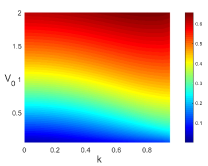
Figure 1: The maximal instability growth rate $\gamma$ as a function of $k$ and $V_{0}$ with $B=0.25$.

IV Instability Results

In this section, by choosing a cut-off $N$ on the number of Fourier modes, we numerically find the spectrum to (5) using the bi-infinite eigenvalue problem (12).

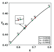
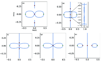
Figure 2: Left panel shows the maximal instability growth rate $\gamma$ as a function of $k$ with $B=0.25$ and $V_{0}=1$. When $k<k_{c}$, the modulation instability appears [one example can be seen in $(a)$ (with $k=0.55$) of the right panel]. At $k=k_{c}$, the ellipse-like curve appears. From $k_{c}$ to $k_{e}$, the dominant instability switches to the ellipse-like instability [one example can be seen in $(d)$ (with $k=0.64$) of the right panel]. At $k=k_{e}$, MI disappears and only the ellipse-like eigenvalues exist. From $k_{e}$ to $k_{g}$, the ellipse-like curve is compressed vertically [as shown in $(f)$ (with $k=0.69$) of the right panel]. An infinity symbol forms at $k_{g}$ (as shown in $(g)$ of the right panel). When $k>k_{g}$, the infinity symbol splits into two isolas drifting away along the real axis [as shown in $(h)$ (with $k=0.8$) of the right panel]. For the right panel, the red dots correspond to $\mu=0$ and the green dots correspond to $\mu=\frac{\pi}{2K(k)}$.

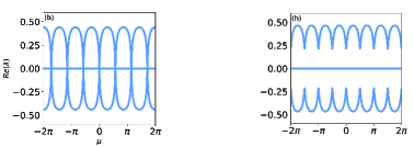
Figure 3: Real part of growth rates as a function of the Floquet parameter $\mu$, where $(b)$ (MI with $k=0.6$) and $(h)$ (isola instability with $k=0.8$) similarly to the left panel of FIG. 2

Figure 4: Eigenfunctions of the isola instability branch for $\mu=\frac{\pi}{2K(k)}$, where $(h)$ is labeled in FIG. 2.

IV.1 From MI to isola instability

Note that the solutions (3) have three free parameters $V_{0}$, $B$ and $k$. FIG. 1 shows the maximal instability growth rate $\gamma$ as a function of $k$ and $V_{0}$ with $B=0.25$. We can see that $\gamma$ increases with $k$ and $V_{0}$ increasing. To study the transition from MI to isola instability, by fixing $V_{0}=1$ and $B=0.25$, we study the dynamics of instabilities with varying $k$, i.e., effectively varying the periodicity of the potential. As shown in FIG. 2, for $0<k<k_{c}=0.63936$, the only instability of the elliptic wave is the MI and the maximal instability growth rate $\gamma$ corresponds to the real eigenvalues with $\mu=\frac{\pi}{2K(k)}$, which implies that the dominant disturbance has twice the period of elliptic wave. A typical example of MI is shown in FIG. 2(a) with $k=0.55\in(0,k_{c})$ and it can be seen that the closure of spectrum that is not on the imaginary axis forms an infinity symbol centered at the spectral plane origin. At $k=k_{c}$, the collisions of eigenvalues on the imaginary axis (at $\pm 0.06202i$), lead to the appearance of an ellipse-like curve. Then from $k_{c}$ to $k_{e}=0.64921$, two types of instability appear, as shown in FIG. 2(d) with $k=0.64$, which shows that a figure 8 is present inside an ellipse-like curve. Therefore from $k_{c}$ to $k_{e}$, the dominant instability switches to the ellipse-like instability, which is not MI (recall that MI involves an unstable band of eigenvalues encompassing the origin), and the dominant disturbance has twice period of elliptic waves. At $k=k_{e}$, a collision of eigenvalues at the origin leads to the disappearance of MI and only the ellipse-like eigenvalues exist. From $k_{e}$ to $k_{g}=0.70863$, the ellipse-like curve is compressed vertically (see FIG. 2(f) with $k=0.69$). Finally, this leads to the formation of an infinity symbol at $k_{g}=0.70863$ (see FIG. 2(g)), again of the MI type.

Increasing $k>k_{g}$, the collision of the eigenvalues with $\mu=0$ (red dots in FIG. 2 (f,g,h)) at the origin (where a Hamiltonian Hopf bifurcation occurs) causes the infinity symbol to subsequently split into two isolas drifting away along the real axis, as shown in Figure 2(h) with $k=0.8$. Now, the dominant instability switches to the isola instability, which is not MI (since the latter involves the spectral plane origin), and the dominant disturbance retains twice the period of the elliptic wave.

For the isola instability, we can observe the following. (a) Similarly to MI, the entire range of the Floquet parameter $\mu$ covers the isola instability branch (as shown in FIG. 3), in contrast to the high-frequency instabilities corresponding to a narrow region of the Floquet parameter $\mu$ (as shown in FIG. 7 below); (b) Differently from the MI, the spectrum of the isola instability has no intersections with the origin and the range of growth rate does not start from zero but from the nonzero eigenvalues with $\mu=0$, as shown in FIG. 3; (c) The maximal instability growth rate corresponds to the real eigenvalues with $\mu=\frac{\pi}{2K(k)}$ (as shown in the green dots of FIG. 2(h)); (d) Such an isola instability branch is called local instability branch in fluids ber1 , since the eigenfunctions associated with such a branch change rapidly in the vicinity of the wave-crest. However, here the eigenfunctions associated with such a branch don’t have such local property (which is a fundamental difference in comparison to ber1 ), as shown in FIG. 4. Therefore, such isola instability in BECs can be deemed to be nontrivially distinct from the local instability branch in fluids.

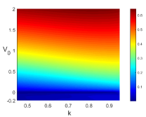
Figure 5: The maximal instability growth rate $\gamma$ as a function of $k$ and $V_{0}$ with $B=0.3$.

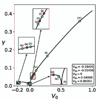
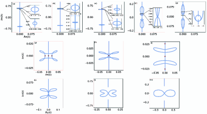
Figure 6: (Left panel) The maximal instability growth rate $\gamma$ as a function of $V_{0}$. When $V_{0}=V_{0f}$, the elliptic solutions are stable. When $-0.19<V_{0}<V_{0b}=-0.18431$, the first bubble dominates the instability (see $(a)$ (with $V_{0}=-0.19$) of the right panel). From $V_{0}$ to $V_{0b}$, the two bubbles approach and collision (see $(b)$ of the right panel). When $V_{0}>V_{0b}$, the two bubbles pass through each other (see $(c)$ (with $V_{0}=-0.18$) of the right panel) and then they fuse together (see $(d)$ (with $V_{0}=-0.01456$) of the right panel) and move toward the origin (see $(e)$ (with $V_{0}=-0.005$) of the right panel). When $0<V_{0}<V_{0j}=0.06063$, a transition between different stability spectra caused by the collision of eigenvalues with $\mu=0$ at the origin happens (see $(g,h,i)$ (with $V_{0}=0.032,0.04009,0.052$) of the right panel). The red dots in $(g,h,i)$ of the right panel correspond to $\mu=0$. When $V_{0}>V_{0j}$, we show three different stability spectra (see $(k,l,m)$ (with $V_{0}=0.1,0.28,0.8$) of the right panel).

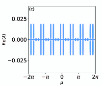
Figure 7: Real part of growth rates as a function of the Floquet parameter $\mu$, where $(c)$ (high-frequency instability) is labeled in the left panel of FIG. 6

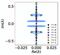
Figure 8: The stability spectrum for the elliptic solutions (3) with respect to $P$-subharmonic perturbations ($k=0.5$, $B=0.3$ and $V_{0}=-0.04$).

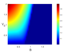
Figure 9: The maximal instability growth rate $\gamma$ as a function of $B$ and $V_{0}$ with $k=0$.

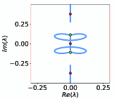
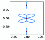
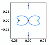
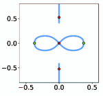
Figure 10: The stability spectrum for the elliptic solutions (3) with $k=0$, $B=0.29$, (from left to right) $V_{0}=0.3$, $V_{0}=0.36166$, $V_{0}=0.4$, $V_{0}=0.48$ and $V_{0}=1$.

IV.2 From MI to high-frequency instability

FIG. 5 shows the maximal instability growth rate $\gamma$ as a function of $k$ and $V_{0}$ with $B=0.3$. We can see that $\gamma$ increases with $k$ and $V_{0}$ increasing. To study the transition from MI to high-frequency instability, by fixing $k=0.5$ and $B=0.3$, we study the dynamics of instabilities with varying $V_{0}$. We note that when $V_{0}=V_{0f}=0$, (1), the problem reduces to the standard defocusing NLS equation. It is well known that all elliptic solutions with $V_{0}=0$ are stable adbe1 . Here we consider the case where $V_{0}\neq 0$. As shown in FIG. 6, when $V_{0}<0$, only the high-frequency instability occurs (see FIG.  6(a,b,c,e)). The high-frequency instability (the corresponding perturbations oscillate in time) develops from a Hamiltonian-Hopf bifurcation: collisions of nonzero, imaginary elements of the stability spectrum ($V_{0}=0$) lead to eigenvalues symmetrically bifurcating from the imaginary axis as $V_{0}$ decreasing, resulting in instability. Specifically, from $-0.19\leqslant V_{0}<V_{0b}=-0.18431$, the first bubble (arising farther away from the origin) dominates the instability (see FIG. 6(a) with $V_{0}=-0.19$). By increasing $V_{0}$ to $V_{0b}$, the two bubbles approach and collide (see FIG. 6(b)). When $V_{0}>V_{0b}$, the two bubbles pass through each other (see FIG. 6(c) with $V_{0}=-0.18$) and subsequently they fuse together (see FIG. 6(d) with $V_{0}=-0.01456$) and move toward the origin (see FIG. 6(e) with $V_{0}=-0.005$). When $0<V_{0}<V_{0j}=0.06063$, the elliptic solutions are modulational stable. We can see the transition between different stability spectra caused by the collision of eigenvalues with $\mu=0$ at the origin (see FIG. 6(g,h,i)). When $V_{0}>V_{0j}$, the modulation instability appears and we show three different stability spectra (see FIG. 6(k,l,m)). Different from MI and isola instability, we can see that the high-frequency instability branch occurs in a narrow region of the Floquet parameter $\mu$ (as shown in FIG. 7), which implies that we may get some useful stability results with respect to subharmonic perturbations. For example, we show that the elliptic solutions (3) (with $k=0.5$, $B=0.3$ and $V_{0}=-0.04$) are stable with respect to $1$-, $2$-, $3$-, $4$- , $5$-, $7$- and $8$- subharmonic perturbations but unstable with respect to the $6$- subharmonic perturbation, as shown FIG. 8.

IV.3 Instability trapped in a standing light wave $(k=0)$

When $k=0$, the elliptic potential $V(x)$ reduces to the trigonometric functions and thus $V(x)$ is a standing light wave. FIG. 9 shows the maximal instability growth rate $\gamma$ as a function of $B$ and $V_{0}$ with $k=0$. We can see that $\gamma$ increases with $V_{0}$ increasing and $B$ decreasing. The MI arises from the collision of the eigenvalues with $\mu=\frac{\pi}{2K(k)}$ at the origin, as shown in FIG. 10. Here, we also note that in FIG. 10 a panel with four petals morphs into a panel with two petals. This is because increasing $V_{0}$ leads to more collisions of imaginary eigenvalues at the origin and the spectral curve is vertically compressed. Besides we note that, solutions (3) with $k=0$ and $b=0.29$ are stable with respect to co-periodic perturbations. When $V_{0}$ is large enough, it can be seen that the maximal instability growth rate corresponds to the real eigenvalues with $\mu=\frac{\pi}{2K(k)}$, as shown in FIG. 10 with $V_{0}=1$.

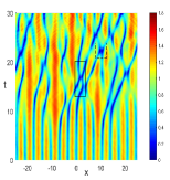
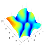
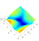
Figure 11: Numerical evolution of the MI resulting in pattern distortion and collisional events (highlighted by boxes on the left panel and zoomed-in at the middle and right panels). The initial condition is solution (3) perturbed by $5\%$ random noise with $k=0.6$, $B=0.25$ and $V_{0}=1$. The amplitude evolution (upper-left); the (solid-line)zoomed-in evolution of the box on the upper-left is shown on the middle panel; the (dotted-line) zoomed-in evolution of the box on the left is shown on the rightmost panel.

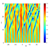
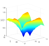
Figure 12: Numerical excitation of the isola instability. The initial condition is solution (3) perturbed by $5\%$ random noise with $k=0.72$, $B=0.25$ and $V_{0}=1$. The amplitude evolution (left); the zoomed-in evolution of the box on the left is shown on the right panel.

IV.4 Dynamical Manifestation of the Instabilities

Having explored the different scenarios of instability, we now turn to direct numerical simulations in order to explore the dynamical byproducts of these instabilities. Starting from the nontrivial phase elliptic solutions (3), we impose random perturbations and visualize the patterns produced by (1) numerically.

The case of dynamical evolution of a modulationally unstable scenario is shown in Fig. 11. One can observe that after an initial stage, the periodic pattern is distorted leading to the emergence of some skewed density dips reminiscent of moving dark (gray) solitary waves; for details of such coherent structures, see the review of djf . As these structures move through the distorted pattern they appear to interact in collision-type events which are somewhat reminiscent of the interactions of dark solitary waves observed, e.g., in the experiments of markus1 ; sengstock ; markus2 . These types of events causing a (deeper) spatio-temporal dip, prior to the colliding patterns re-emerging are highlighted in two boxes in Fig. 11 whose evolution is presented in more detail in the additional panels of the figure.

Interestingly, and as perhaps may be expected by the similar nature of the relevant instability (although the isola instability is detached from the spectral plane origin), the dynamics of the isola instability is similar to that of MI. Indeed, the relevant dynamical manifestations can be seen in Fig. 12. Here, too, it is evident that the distortion of the pattern leads to a number of waves that propagate along skewed lines in the space-time (left) panel of the figure. The zoom-in to the box of the left panel is once again shown in the right panel, illustrating a space-time collisional type event before the participating waves once again separate. It is relevant to note here that similar results to those of Figs. 11-12 arise in the case of $k=0$, i.e., for a trigonometric standing wave of light (results not shown here).

Finally, it is interesting to point out the fundamental difference of the high-frequency instability, in comparison, e.g., with those of Figs. 11-12 above. A prototypical example of the high-frequency instability is shown in Fig. 13. We can see that the instability is manifested through the propagation of high-wavenumber unstable modes which, in turn, are weakly perturbing the (deeper) density dips of the original configuration. Nevertheless, the latter persist, avoiding the more intense collisional events described above.

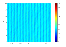
Figure 13: The initial condition is solution (3) perturbed by $5\%$ random noise with $k=0.5$, $B=0.3$ and $V_{0}=-0.1$.

V Conclusions & Future Challenges

The instabilities of the nontrivial phase elliptic solutions in a repulsive Bose-Einstein condensate (BEC) with a periodic potential have been studied. Based on the defocusing nonlinear Schrödinger (NLS) equation with an elliptic function potential based on a sequence of fundamental earlier works bec11 ; bec12 ; bec13 ; bec14 , the MI, the similar to it isola instability (on the real line) and the rather different high-frequency instability have been observed numerically and have been elucidated quantitatively. With varying parameters in solutions and equation, instability transitions occur, e.g., through a Hamiltonian Hopf bifurcation. Specifically, (i) increasing $k$, we have observed that the MI switches to the isola instability and the dominant disturbances have twice elliptic wave’s period, corresponding to a Floquet exponent $\mu=\frac{\pi}{2K(k)}$. The isola instability arises from the collision of spectral elements at the origin with $\mu=0$; (ii) with varying $V_{0}$, the transition between the MI and high-frequency instability occurs. Different from the MI and isola instability where the collisions of spectral elements happen at the origin, the high-frequency instability arises from pairwise collisions of nonzero, imaginary elements of the stability spectrum; (iii) in the limit of sinusoidal potential, with varying $V_{0}$, we have shown the MI occurs from a collision of eigenvalues with $\mu=\frac{\pi}{2K(k)}$ at the origin; (iv) the dynamical evolution of the relevant instabilities has been elucidated, notably leading in the case of the MI and isola instabilities to distortion of the patterns and events resembling the collision of dark (gray) solitary waves.

Admittedly, since the emergence of these fundamental works bec11 ; bec12 ; bec13 ; bec14 , numerous developments have arisen in higher-dimensional BECs bec2-3 , in multi-component condensates ueda1 ; ueda2 , as well as in the context of long-range interactions lahaye . Extending the present considerations to these progressively more and more accessible settings would be a natural next step for future studies.

Acknowledgements This work has been supported by the Fundamental Research Funds of the Central Universities (No. 230201606500048) and the National Natural Science Foundation of China under Grant No.12205029. The work of P.G.K is supported by the US National Science Foundation under Grants No. PHY-2110030 and DMS-2204702).

References

- (1) C. J. Pethick and H. Smith, Bose-Einstein condensation in dilute gases, Cambridge University Press (Cambridge, 2008).
- (2) L. P. Pitaevskii and S. Stringari, Bose-Einstein Condensation and Superfluidity, Oxford University Press (Oxford, 2016).
- (3) O. Morsch and M. Oberthaler, Rev. Mod. Phys. 78, 179 (2006).
- (4) E. Kengne, W. M. Liu, and B. A. Malomed, Phy. Rep. 899, 1 (2021).
- (5) P. G. Kevrekidis, D. J. Frantzeskakis, and R. Carretero-González, The Defocusing Nonlinear Schrödinger Equation: From Dark Solitons to Vortices and Vortex Rings, SIAM (Philadelphia, 2015).
- (6) B. P. Anderson and M. A. Kasevich, Science 282, 1686 (1998).
- (7) E. W. Hagley, L. Deng, M. Kozuma, J. Wen, K. Helmerson, S. L. Rolston, and W. D. Phillips, Science 283, 1706 (1999).
- (8) Y. B. Ovchinnikov, J. H. Muller, M. R. Doery, E. J. D. Vredenbregt, K. Helmerson, S. L. Rolston, and W. D. Phillips, Phys. Rev. Lett. 83, 284 (1999).
- (9) D. Jaksch, C. Bruder, J. I. Cirac, C. W. Gardiner, and P. Zoller, Phys. Rev. Lett. 81, 3108 (1998).
- (10) G. K. Brennen, C. M. Caves, P. S. Jessen, and I. H. Deutsch, Phys. Rev. Lett. 82, 1060 (1999).
- (11) D. I. Choi and Q. Niu, Phys. Rev. Lett. 82, 2022 (1999).
- (12) L. D. Carr and J. Brand, Phys. Rev. A 70, 033607 (2004).
- (13) Y. S. Kivshar and G. P. Agrawal, Optical Solitons: From Fibers to Photonic Crystals (Academic, New York, 2003).
- (14) T. J. Alexander, E. A. Ostrovskaya, and Y. S. Kivshar, Phys. Rev. Lett. 96, 040401 (2006).
- (15) N. A. Kostov, V. Z. Enol’skii, V. S. Gerdjikov, V. V. Konotop, and M. Salerno, Phy. Rev. E 70, 056617 (2004).
- (16) J. C. Bronski, L. D. Carr, R. C. Gonzlez, B. Deconinck, J. N. Kutz, and K. Promislow, Phy. Rev. E 64, 056615 (2001).
- (17) J. C. Bronski, L. D. Carr, B. Deconinck, and J. N. Kutz, Phy. Rev. E 63, 036612 (2001).
- (18) J. C. Bronski, L. D. Carr, B. Deconinck, and J. N. Kutz, Phy. Rev. Lett. 86, 1402 (2001).
- (19) J. C. Bronski and Z. Rapti, Dynamics of Partial Differential Equations 2, 335 (2005).
- (20) P. G. Kevrekidis and D.J. Frantzeskakis, Mod. Phys. Lett. B 18, 173 (2004).
- (21) K. E. Strecker, G. B. Partridge, A. G. Truscott, and R. G. Hulet, Nature 417, 150 (2002).
- (22) J. H. V. Nguen, D. Luo, and R. G. Hulet, Science 356, 422 (2017).
- (23) P. J. Everitt, M. A. Sooriyabandara, M. Guasoni, P. B. Wigley, C. H. Wei, G. D. McDonald, K. S. Hardman, P. Manju, J. D. Close, C. C. N. Kuhn, S. S. Szigeti, Y. S. Kivshar, and N. P. Robins, Phys. Rev. A 96, 041601(R) (2017).
- (24) C. A. Chen and C. L. Hung, Phys. Rev. Lett. 125, 250401 (2020).
- (25) A. Smerzi, A. Trombettoni, P. G. Kevrekidis, and A. R. Bishop, Phys. Rev. Lett. 89, 170402 (2002).
- (26) F. S. Cataliotti, L. Fallani, F. Ferlaino, C. Fort, P. Maddaloni, and M. Inguscio, New J. Phys. 5, 71 (2003).
- (27) J. Meier, G. I. Stegeman, D. N. Christodoulides, Y. Silberberg, R. Morandotti, H. Yang, G. Salamo, M. Sorel, and J. S. Aitchison, Phys. Rev. Lett. 92, 163902 (2004).
- (28) N. Boechler, G. Theocharis, S. Job, P. G. Kevrekidis, Mason A. Porter, and C. Daraio, Phys. Rev. Lett. 104, 244302 (2010).
- (29) F. Dalfovo, S. Giorgini, L. P. Pitaevskii, and S. Stringari, Rev. Mod. Phys. 71, 463 (1999).
- (30) L. D. Carr, C. W. Clark, and W. P. Reinhardt, Phys. Rev. A 62, 063610 (2000).
- (31) T. B. Benjamin and J. Feir. J. Fluid Mech. 27, 417 (1967).
- (32) V. V. Konotop and M. Salerno, Phys. Rev. A 65, 021602 (2002).
- (33) L. Salasnich, A. Parola, and L. Reatto, Phys. Rev. Lett. 91, 080405 (2003).
- (34) G. Theocharis, Z. Rapti, P. G. Kevrekidis, D. J. Frantzeskakis, and V. V. Konotop, Phys. Rev. A 67, 063610 (2003).
- (35) L. D. Carr and J. Brand, Phys. Rev. Lett. 92, 040401 (2004).
- (36) S. Ro jas-Ro jas, R. A. Vicencio, M. I. Molina, and F. Kh. Abdullaev, Phys. Rev. A 84, 033621 (2011).
- (37) A. Hasegawa, Opt. Lett. 9, 288 (1984).
- (38) K. Tai, A. Hasegawa, and A. Tomita, Phys. Rev. Lett. 56, 135 (1986).
- (39) S. Trillo and S. Wabnitz, Opt. Lett. 16, 986 (1991).
- (40) S. Coen and M. Haelterman, Phys. Rev. Lett. 79, 4139 (1997).
- (41) M. Peccianti, C. Conti, G. Assanto, A. De Luca, and C. Umeton, Nature 432, 733 (2004).
- (42) Y. V. Kartashov and D. V. Skryabin, Optica 3, 1228 (2016).
- (43) E. Kengne, W. M. Liu, L. Q. English, and B. A. Malomed, Phys. Rep. 982, 1 (2022).
- (44) T. Hansson, D. Modotto, and S. Wabnitz, Phys. Rev. A 88, 023819 (2013).
- (45) Y. S. Kivshar and M. Peyrard, Phys. Rev. A 46, 3198 (1992).
- (46) B. Deconinck and K. Oliveras. J. Fluid Mech. 675, 141 (2011).
- (47) R. P. Creedon, B. Deconinck, and O. Trichtchenko. J. Fluid Mech. 937, A24 (2022).
- (48) V. M. Hur and Z. Yang. Unstable stokes waves. arXiv:2010.10766 (2022).
- (49) B. Deconinck, S. A. Dyachenko, P. M. Lushnikov, and A. Semenova, arXiv:2211.05473 (2022).
- (50) K. B. Dysthe and K. Trulsen, Phys. Scr. T82, 48 (1999).
- (51) A. I. Dyachenko and V. E. Zakharov, JETP Lett. 81, 255 (2005).
- (52) J. M. Dudley, F. Dias, M. Erkintalo, and G. Genty, Nat. Photonics 8, 755 (2014).
- (53) M. Onorato, S. Residori, U. Bortolozzo, A. Montina, and F. T. Arecchi, Phys. Rep. 528, 47 (2013).
- (54) F. Baronio, M. Conforti, A. Degasperis, S. Lombardo, M. Onorato, and S. Wabnitz, Phys. Rev. Lett. 113, 034101 (2014).
- (55) B. Deconinck and J. N. Kutz, J. Comp. Physics 219, 296 (2006).
- (56) N. Bottman, B. Deconinck, and M. Nivala, J. Phys. A 44, 285201 (2011).
- (57) D. J. Frantzeskakis, J. Phys. A 43, 213001 (2010).
- (58) A. Weller, J. P. Ronzheimer, C. Gross, J. Esteve, M. K. Oberthaler, D. J. Frantzeskakis, G. Theocharis, and P. G. Kevrekidis, Phys. Rev. Lett. 101, 130401 (2008).
- (59) S. Stellmer, C. Becker, P. Soltan-Panahi, E. M. Richter, S. Dörscher, M. Baumert, J. Kronjäger, K. Bongs, and K. Sengstock, Phys. Rev. Lett. 101, 120406 (2008).
- (60) G. Theocharis, A. Weller, J. P. Ronzheimer, C. Gross, M. K. Oberthaler, P. G. Kevrekidis, and D. J. Frantzeskakis, Phys. Rev. A 81, 063604 (2010).
- (61) Y. Kawaguchi and M. Ueda, Phys. Rep. 520, 253 (2012).
- (62) D. M. Stamper-Kurn and M. Ueda, Rev. Mod. Phys. 85, 1191 (2013).
- (63) T. Lahaye, C. Menotti, L. Santos, M. Lewenstein, and T. Pfau, Rep. Prog. Phys. 72, 126401 (2009).