Hierarchical Wilson-Cowan Models and Connection Matrices

Abstract

This work aims to study the interplay between the Wilson-Cowan model and the connection matrices. These matrices describe the cortical neural wiring, while the Wilson-Cowan equations provide a dynamical description of neural interaction. We formulate the Wilson-Cowan equations on locally compact Abelian groups. We show that the Cauchy problem is well-posed. We then select a type of group that allows us to incorporate the experimental information provided by the connection matrices. We argue that the classical Wilson-Cowan model is incompatible with the small-world property. A necessary condition to have this property is that the Wilson-Cowan equations be formulated on a compact group. We propose a $p$-adic version of the Wilson-Cowan model, a hierarchical version in which the neurons are organized into an infinite rooted tree. We present several numerical simulations showing that the $p$-adic version matches the predictions of the classical version in relevant experiments. The $p$-adic version allows the incorporation of the connection matrices into the Wilson-Cowan model. We present several numerical simulations using a neural network model that incorporates a $p$-adic approximation of the connection matrix of the cat cortex.

Keywords— Wilson-Cowan Model, Connection matrices, $p$-adic numbers, Small-world networks.

1 Introduction

This work explores the interplay between the Wilson-Cowan models, the connection matrices, and the non-Archimedean models of complex systems.

The Wilson-Cowan model describes the evolution of excitatory and inhibitory activity in a synaptically coupled neuronal network. The model is given by the following system of non-linear integro-differential evolution equations:

$$\begin{array}[c]{ll}\tau\frac{\partial E(x,t)}{\partial t}=&-E(x,t)+\\ &\\ &\left(1-r_{E}E(x,t)\right)S_{E}\left(w_{EE}\left(x\right)\ast E(x,t)-w_{EI}\left(x\right)\ast I(x,t)+h_{E}\left(x,t\right)\right)\\ &\\ \tau\frac{\partial I(x,t)}{\partial t}=&-I(x,t)+\\ &\\ &\left(1-r_{I}I(x,t)\right)S_{I}\left(w_{IE}\left(x\right)\ast E(x,t)-w_{II}(x)\ast I(x,t)+h_{I}\left(x,t\right)\right),\end{array}$$

where $E(x,t)$ is a temporal coarse-grained variable describing the proportion of excitatory neuron firing per unit of time at position $x\in\mathbb{R}$ at the  instant $t\in\mathbb{R}_{+}$. Similarly the variable $I(x,t)$ represents the activity of the inhibitory population of neurons. The main parameters of the model are the strength of the connections between each subtype of population ($w_{EE}$, $w_{IE}$, $w_{EI}$, $w_{II}$) and the strength of input to each subpopulation ($h_{E}\left(x,t\right)$, $h_{I}\left(x,t\right)$). This model generates a diversity of dynamical behaviors that are representative of observed activity in the brain, like multistability, oscillations, traveling waves, and spatial patterns, see, e.g., [1]-[2], [3] and the references therein.

We formulate the Wilson-Cowan model on Abelian, locally compact topological groups. The classical model corresponds to the group $(\mathbb{R},+)$. In this framework, using classical techniques on semilinear evolution equations, see e.g. [4]-[5], we show that the corresponding Cauchy problem is locally well-posed, and if $r_{E}=r_{I}=0$, it is globally well-posed, see Theorem 2.5. This last condition corresponds to the case of two coupled perceptrons.

Nowadays, there is a large amount of experimental data about the connection matrices of the cerebral cortex of invertebrates and mammalians. Based on these data, several researchers hypothesized that cortical neural networks are arranged in fractal or self-similar patterns and have the small-world property, see, e.g., [6]-[19], and the references therein. The connection matrices provide a static view of the neural connections.

The investigation of the relationships between the Wilson-Cowan model and the connection matrices is quite natural, since model was proposed to explain the cortical dynamics, while the matrices describe the functional geometry of the cortex. We initiate this study here.

A network having the small-world property necessarily has long-range interactions; see Section 3. In the Wilson-Cowan model, the kernels ($w_{EE}$, $w_{IE}$, $w_{EI}$, $w_{II}$) describing the neural interactions are Gaussian in nature, so only short-range interactions may occur. For practical purposes, these kernels have compact support. On the other hand, the Wilson-Cowan model on a general group requires that the kernels be integrable; see Section 2. We argue that $G$ must be compact to satisfy the small-world property. Under this condition, any continuous kernel is integrable. Wilson and Cowan formulated their model on the group $(\mathbb{R},+)$. The only compact subgroup of this group is the trivial one. The small-world property is, therefore, incompatible with the classical Wilson-Cowan model.

It is worth noting that the absence of non-trivial compact subgroups in $(\mathbb{R},+)$ is a consequence of the Archimedean axiom (the absolute value is  not bounded on the integers). Therefore, to avoid this problem, we can replace $\mathbb{R}$ with a non-Archimedean field, which is a field where the Archimedean axiom is no valid. We selected the field of the $p$-adic numbers. This field has infinitely many compact subgroups, the balls with center at the origin. We selected the unit ball, the ring of $p$-adic numbers $\mathbb{Z}_{p}$. The $p$-adic integers are organized in an infinite rooted tree. We use this hierarchical structure as the topology for our $p$-adic version of the Wilson-Cowan model. In principle, we could use other groups, such as the classical compact groups, to replace $(\mathbb{R},+)$, but it is also essential to have a rigorous study of the discretization of the model. For the group $\mathbb{Z}_{p}$, this task can be performed using standard approximation techniques for evolutionary equations, see, e.g., [5, Section 5.4].

The $p$-adic Wilson-Cowan model admits good discretizations. Each discretization corresponds to a system of non-linear integro-differential equations on a finite rooted tree. We show that the solution of the Cauchy problem of this discrete system provides a good approximation to the solution of the Cauchy problem of the $p$-adic Wilson-Cowan model, see Theorem 4.3.

We provide extensive numerical simulations of $p$-adic Wilson-Cowan models. In Section 5, we present three numerical simulations showing that the $p$-adic models provide a similar explanation to the numerical experiments presented in [2]. In these experiments the kernels ($w_{EE}$, $w_{IE}$, $w_{EI}$, $w_{II}$) were chosen to have similar properties to the kernels used in [2]. In Section 6, we consider the problem of how to integrate the connection matrices into the $p$-adic Wilson-Cowan model. This fundamental scientific task aims to use the vast amount of data on maps of neural connections to understand the dynamics of the cerebral cortex of invertebrates and mammalians. We show that the connection matrix of the cat cortex can be well approximated by a $p$-adic kernel $K_{r}(x,y)$. We then replace the excitatory-excitatory relation term $w_{EE}\ast E$ by $\int_{\mathbb{Z}_{p}}K_{r}(x,y)E(y)dy$ but keep the other kernels as in Simulation 1 presented in Section 5. The response of this network is entirely different from that given in Simulation 1. For the same stimulus, the response of the last network exhibits very complex patterns, while the response of the network presented in Simulation 1 is simpler.

The $p$-adic analysis has shown to be the right tool in the construction of a wide variety of models of complex hierarchic systems, see, e.g., [20]-[28], and the references therein. Many of these models involve abstract evolution equations of the type $\partial_{t}u+\boldsymbol{A}u=F(u)$. In these models, the discretization of the operator $\boldsymbol{A}$ is an ultrametric matrix $A_{l}=\left[a_{ij}\right]_{i,j\in G_{l}}$, where $G_{l}$ is a finite rooted tree with $l$ levels and $p^{l}$ branches, here $p$ is a fixed prime number, see the numerical simulations in [27]-[28]. Locally, the connection matrices look very similar to the matrices $A_{l}$. The problem of approximating large connection matrices by ultrametric matrices is an open problem.

2 An abstract version of the Wilson-Cowan Equations

In this section, we formulate the Wilson-Cowan model on locally compact topological groups and study the well-posedness of the Cauchy problem attached to these equations.

2.1 Wilson-Cowan Equations on Abelian locally compact topological groups

Let $\left(\mathcal{G},+\right)$ be an Abelian, locally compact topological group. Let $d\mu$ be a fixed Haar measure on $\left(\mathcal{G},+\right)$. The basic example is $\left(\mathbb{R}^{N},+\right)$, the $N$-dimensional Euclidean space considered as an additive group. In this case $d\mu$ is the Lebesgue measure of $\mathbb{R}^{N}$.

Let $L^{\infty}\left(\mathcal{G}\right)$ be the $\mathbb{R}$-vector space of functions $f:\mathcal{G}\rightarrow\mathbb{R}$  satisfying

$$\left\|f\right\|_{\infty}=\sup_{x\in\mathcal{G\smallsetminus A}}\left|f\left(x\right)\right|<\infty,$$

where $\mathcal{A}$ is a subset of $\mathcal{G}$ with measure zero. Let $L^{1}\left(\mathcal{G}\right)$ be the $\mathbb{R}$-vector space of functions $f:\mathcal{G}\rightarrow\mathbb{R}$  satisfying

$$\left\|f\right\|_{1}={\displaystyle\int\limits_{\mathcal{G}}}\left|f\left(x\right)\right|d\mu<\infty.$$

For a fixed $w\in L^{1}\left(\mathcal{G}\right)$, the mapping

$$\begin{array}[c]{ccc}L^{\infty}\left(\mathcal{G}\right)&\rightarrow&L^{\infty}\left(\mathcal{G}\right)\\ &&\\ f\left(x\right)&\rightarrow&\left(w\ast f\right)\left(x\right)=\int_{\mathcal{G}}\text{ }w\left(x-y\right)f\left(y\right)d\mu(y)\end{array}$$

is a well-defined  linear bounded operator satisfying

$$\left\|w\ast f\right\|_{\infty}\leq\left\|w\right\|_{1}\left\|f\right\|_{\infty}.$$

Remark 2.1

• We recall that $f:\mathbb{R}\rightarrow\mathbb{R}$ is called a Lipschitz function if there is positive constant $L(f)$ such that $\left|f(x)-f(y)\right|\leq L(f)\left|x-y\right|$ for all $x$ and $y$.

• Given $\mathcal{X}$, $\mathcal{Y}$, Banach spaces, we denote by $\mathcal{C}(\mathcal{X},\mathcal{Y})$ the space of continuous functions from $\mathcal{X}$ to $\mathcal{Y}$.

• If $\mathcal{Y}=\mathbb{R}$, we use the simplified notation $\mathcal{C}(\mathcal{X})$.

We fix two bounded Lipschitz functions $S_{E}$, $S_{I}$ satisfying

$$S_{E}\left(0\right)=S_{I}\left(0\right)=0.$$

We also fix $w_{EE}$, $w_{IE}$, $w_{EI}$, $w_{II}\in L^{1}\left(\mathcal{G}\right)$, and $h_{E}\left(x,t\right)$, $h_{I}\left(x,t\right)\in\mathcal{C}(\left[0,\infty\right],L^{\infty}\left(\mathcal{G}\right))$.

The Wilson-Cowan model on $\mathcal{G}$ is given by the following system of non-linear integron-differential evolution equations:

$$\tau\frac{\partial E(x,t)}{\partial t} =-E(x,t)+$$

$$\left(1-r_{E}E(x,t)\right)S_{E}\left(w_{EE}\left(x\right)\ast E(x,t)-w_{EI}\left(x\right)\ast I(x,t)+h_{E}\left(x,t\right)\right)$$

$$\tau\frac{\partial I(x,t)}{\partial t} =-I(x,t)+$$

$$\left(1-r_{I}I(x,t)\right)S_{I}\left(w_{IE}\left(x\right)\ast E(x,t)-w_{II}(x)\ast I(x,t)+h_{I}\left(x,t\right)\right),$$

where $\ast$ denotes the convolution in the space variables and $r_{E}$, $r_{I}\in\mathbb{R}$.

The space $\mathcal{X}:=L^{\infty}\left(\mathcal{G}\right)\times L^{\infty}\left(\mathcal{G}\right)$ endowed with the norm

$$\left\|\left(f_{1},f_{2}\right)\right\|=\max\left\{\left\|f_{1}\right\|_{\infty},\left\|f_{2}\right\|_{\infty}\right\}$$

is a real Banach space.

Given $f=\left(f_{1},f_{2}\right)\in\mathcal{X}$, and $P(x)$, $Q(x)\in L^{\infty}\left(\mathcal{G}\right)$, we set

$$\boldsymbol{F}_{E}(f)=S_{E}\left(w_{EE}(x)\ast f_{1}(x)-w_{EI}(x)f_{2}(x)+P(x)\right),$$ (2.1)

and

$$\boldsymbol{F}_{I}(f)=S_{I}\left(w_{IE}(x)\ast f_{1}(x)-w_{II}(x)\ast f_{2}(x)+Q(x)\right).$$ (2.2)

We also set

$$\begin{array}[c]{ccc}\mathcal{X}&\rightarrow&\mathcal{X}\\ &&\\ f&\rightarrow&\boldsymbol{H}(f),\end{array}$$

where $\boldsymbol{H}(f)=\left(\boldsymbol{H}_{E}(f),\boldsymbol{H}_{I}(f)\right)$ and

$$\boldsymbol{H}_{E}(f)=(1-r_{E}f_{1})\boldsymbol{F}_{E}(f)\text{, }\boldsymbol{H}_{I}(f)=(1-r_{I}f_{2})\boldsymbol{F}_{I}(f).$$ (2.3)

Remark 2.2

We say that $\boldsymbol{H}$  is Lipschitz continuous (or globally Lipschitz) if there is a constant $L(\boldsymbol{H})$ such that $\left\|\boldsymbol{H}(f)-\boldsymbol{H}(g)\right\|\leq L(\boldsymbol{H})\left\|f-g\right\|$, for all $f$, $g\in\mathcal{X}$. We also say that $\boldsymbol{H}$  is locally Lipschitz continuous (or locally Lipschitz) if for every $h\in\mathcal{X}$ there exist a ball $B_{R}\left(h\right)=\left\{f\in\mathcal{X};\left\|f-h\right\|<R\right\}$ such that $\left\|\boldsymbol{H}(f)-\boldsymbol{H}(g)\right\|\leq L(R,h)\left\|f-g\right\|$ for all $f$, $g\in B_{R}\left(h\right)$. Since $\mathcal{X}$ is a vector space, without loss of generality, we can assume that $h=0$.

Lemma 2.3

With the above notation. If $r_{I}\neq 0$ or $r_{E}\neq 0$, the $\boldsymbol{H}:\mathcal{X}\rightarrow\mathcal{X}$ is a well-defined locally Lipschitz mapping. If $r_{I}=$ $r_{E}=0$, then $\boldsymbol{H}:\mathcal{X}\rightarrow\mathcal{X}$ is a well-defined globally Lipschitz mapping.

Proof. We first notice that for $f$, $g\in\mathcal{X}$, by using that $S_{E}$ is Lipschitz,

$$\left|\left(\boldsymbol{F}_{E}(f)-\boldsymbol{F}_{E}(g)\right)(x)\right|$$

$$\leq L\left(S_{E}\right)\left|w_{EE}(x)\ast\left(f_{1}(x)-g_{1}\left(x\right)\right)-w_{EI}(x)\left(f_{2}(x)-g_{2}(x)\right)\right|$$

$$\leq L\left(S_{E}\right)\left\{\left\|w_{EE}\right\|_{1}\left\|f_{1}-g_{1}\right\|_{\infty}+\left\|w_{EI}\right\|_{1}\left\|f_{2}-g_{2}\right\|_{\infty}\right\}$$

$$\leq L\left(S_{E}\right)\max\left\{\left\|w_{EE}\right\|_{1},\left\|w_{EI}\right\|_{1}\right\}\left\|f-g\right\|,$$

which implies that

$$\left\|\boldsymbol{F}_{E}(f)-\boldsymbol{F}_{E}(g)\right\|\leq L(\boldsymbol{F}_{E})\left\|f-g\right\|.$$ (2.4)

Similarly

$$\left\|\boldsymbol{F}_{I}(f)-\boldsymbol{F}_{I}(g)\right\|\leq L(\boldsymbol{F}_{I})\left\|f-g\right\|,$$ (2.5)

where $L(\boldsymbol{F}_{I})=L(S_{I})\max\left\{\left\|w_{IE}\right\|_{1},\left\|w_{II}\right\|_{1}\right\}$.

Now, by using estimation (2.4),  and the fact that $\left\|\boldsymbol{F}_{E}(f)\right\|\leq\left\|S_{E}\right\|_{\infty}$,

$$\left\|\boldsymbol{H}_{E}(f)-\boldsymbol{H}_{E}(g)\right\|=\left\|(1-r_{E}f_{1})\boldsymbol{F}_{E}(f)-(1-r_{E}g_{1})\boldsymbol{F}_{E}(g)\right\|=$$

$$\left\|\left(1-r_{E}f_{1}\right)\left(\boldsymbol{F}_{E}(f)-\boldsymbol{F}_{E}(g)\right)-r_{E}\boldsymbol{F}_{E}(g)\left(f_{1}-g_{1}\right)\right\|$$

$$\leq\left(1+\left|r_{E}\right|\left\|f_{1}\right\|_{\infty}\right)\left\|\boldsymbol{F}_{E}(f)-\boldsymbol{F}_{E}(g)\right\|+\left|r_{E}\right|\left\|\boldsymbol{F}_{E}(f)\right\|\left\|f_{1}-g_{1}\right\|_{\infty}$$

$$\leq\left\{\left(1+\left|r_{E}\right|\left\|f_{1}\right\|_{\infty}\right)L(\boldsymbol{F}_{E})+\left|r_{E}\right|\left\|S_{E}\right\|_{\infty}\right\}\left\|f-g\right\|.$$

By a similar reasoning using estimation (2.5), one gets that

$$\left\|\boldsymbol{H}_{I}(f)-\boldsymbol{H}_{I}(g)\right\|_{\infty}\leq\left(\left(1+\left|r_{I}\right|\left\|f_{2}\right\|_{\infty}\right)L(\boldsymbol{F}_{I})+\left|r_{I}\right|\left\|S_{I}\right\|_{\infty}\right)\left\|f-g\right\|,$$

and consequently

$$\left\|\boldsymbol{H}(f)-\boldsymbol{H}(g)\right\| =\max\left\{\left\|\boldsymbol{H}_{E}(f)-\boldsymbol{H}_{E}(g)\right\|_{\infty},\left\|\boldsymbol{H}_{I}(f)-\boldsymbol{H}_{I}(g)\right\|_{\infty}\right\}$$

$$\leq\left(A\left(1+B\left\|f\right\|_{\infty}\right)+C\right)\left\|f-g\right\|,$$ (2.6)

where

$$A:=\max\left\{L(\boldsymbol{F}_{E}),L(\boldsymbol{F}_{I})\right\},B:=\left\{\left|r_{E}\right|,\left|r_{I}\right|\right\},C:=\max\left\{\left|r_{E}\right|\left\|S_{E}\right\|_{\infty},\left|r_{I}\right|\left\|S_{I}\right\|_{\infty}\right\}.$$

In the case $r_{E}=r_{I}=0$, estimation (2.6) takes the form

$$\left\|\boldsymbol{H}(f)-\boldsymbol{H}(g)\right\|\leq A\left\|f-g\right\|.$$ (2.7)

Which in turn implies that for $f\in\mathcal{X},$

$$\left\|\boldsymbol{H}(f)\right\|\leq\left\|\boldsymbol{H}(f)-\boldsymbol{H}(0)\right\|+\left\|\boldsymbol{H}(0)\right\|\leq A\left\|f\right\|+\left\|\left(\boldsymbol{F}_{E}\left(0\right),\boldsymbol{F}_{I}\left(0\right)\right)\right\|$$ (2.8)

$$=A\left\|f\right\|+\left\|\left(S_{E}\left(0\right),S_{I}\left(0\right)\right)\right\|\leq A\left\|f\right\|+\max\left\{\left\|S_{E}\right\|_{\infty},\left\|S_{I}\right\|_{\infty}\right\}<\infty.$$

Then estimations (2.8)- (2.7) imply that $\boldsymbol{H}$ is a well-defined globally Lipschitz mapping.

We now consider the case $r_{I}\neq 0$ or $r_{E}\neq 0$. Take $f$, $g\in B_{R}\left(0\right)$, for some $R>0$. Then $\left\|f_{1}\right\|_{\infty}<R$, and estimation (2.6) takes the form

$$\left\|\boldsymbol{H}(f)-\boldsymbol{H}(g)\right\| \leq\left\{\left(1+\left|r_{E}\right|R\right)L(\boldsymbol{F}_{E})+\left|r_{E}\right|\left\|S_{E}\right\|_{\infty}\right\}\left\|f-g\right\|$$

$$\leq C\left\|f-g\right\|\text{, for }f,g\in B_{R}\left(0\right)\text{.}$$

Which implies that

$$\left\|\boldsymbol{H}(f)\right\|\leq\left\|\boldsymbol{H}(f)-\boldsymbol{H}(0)\right\|+\left\|\boldsymbol{H}(0)\right\|\leq C\left\|f\right\|+\max\left\{\left\|S_{E}\right\|_{\infty},\left\|S_{I}\right\|_{\infty}\right\}<\infty.$$ (2.9)

Then, the restriction of $\boldsymbol{H}$ to $B_{R}\left(0\right)\times B_{R}\left(0\right)$ is a well-defined Lipschitz mapping.   

The estimations given in Lemma 2.3 are still valid for functions depending continuously on a parameter $t$. More precisely, take $T>0$ and $f_{i}\in\mathcal{C}\left(\left[0,T\right],\mathcal{U}\right)$, for $i=1,2$, where $\mathcal{U}\subset$ $L^{\infty}\left(\mathcal{G}\right)$ is an open subset. We assume that

$$\left(0,T\right)\subset f_{i}^{-1}\left(\mathcal{U}\right)\text{, for }i=1,2.$$

We use the notation $f_{i}=f_{i}\left(\cdot,t\right)$, where $t\in\left[0,T\right]$,  $i=1,2$. We replace $P(x)$ by $h_{E}\left(x,t\right)$ and $Q(x)$ by $h_{I}\left(x,t\right)$, with $h_{E}\left(x,t\right)$, $h_{I}\left(x,t\right)\in\mathcal{C}\left(\left[0,\infty\right),L^{\infty}\left(\mathcal{G}\right)\right)$. We denote the corresponding maping $\boldsymbol{H}\left(f\right)$ as $\boldsymbol{H}\left(f,s\right)$. We also set $\mathcal{X}_{\mathcal{U},T}:=\left[0,T\right]\times\mathcal{U}$.

Lemma 2.4

With the above notation, the following assertions hold:

(i) The mapping $\boldsymbol{H}:\mathcal{X}_{\mathcal{U},T}\times\mathcal{X}_{\mathcal{U},T}\rightarrow\mathcal{X}$ is continuous, and for each $t\in\left(0,T\right)$ and each $h\in\mathcal{U}$ there exist $R>0$ and $L<\infty$ such that

$$\left\|\boldsymbol{H}\left(f,s\right)-\boldsymbol{H}\left(g,s\right)\right\|\leq L\left\|f-g\right\|\text{ for }f,g\in B_{R}(h)\text{, }s\in\left[0,t\right].$$

(ii) For $t\in\left(0,T\right)$, $f\in\mathcal{U}\times\mathcal{U}$,

$${\displaystyle\int\nolimits_{0}^{t}}\left\|\boldsymbol{H}\left(f,s\right)\right\|ds<\infty.$$

Proof. (i) it follows from Lemma 2.3. By estimations (2.8) and (2.9), $\left\|\boldsymbol{H}\left(f,s\right)\right\|$ is bounded by a positive constant $C$ depending on $R$, then

$${\displaystyle\int\nolimits_{0}^{t}}\left\|\boldsymbol{H}\left(f,s\right)\right\|ds<CT.$$

 

2.2 The Cauchy problem

With the above notation, the Cauchy problem for the abstract Wilson-Cowan system takes the following form

$$\left\{\begin{array}[c]{ll}\tau\frac{\partial}{\partial t}\left[\begin{array}[c]{c}E\left(x,t\right)\\ I\left(x,t\right)\end{array}\right]+\left[\begin{array}[c]{c}E\left(x,t\right)\\ I\left(x,t\right)\end{array}\right]=\boldsymbol{H}(\left[\begin{array}[c]{c}E\left(x,t\right)\\ I\left(x,t\right)\end{array}\right]),&x\in\mathcal{G}\text{, }t\geq 0\\ &\\ \left[\begin{array}[c]{c}E\left(x,0\right)\\ I\left(x,0\right)\end{array}\right]=\left[\begin{array}[c]{c}E_{0}\left(x\right)\\ I_{0}\left(x\right)\end{array}\right]\in\mathcal{X}.&\end{array}\right.$$ (2.10)

Theorem 2.5

(i) There exist $T_{0}\in\left(0,T\right]$ depending on $\left[\begin{array}[c]{c}E_{0}\left(x\right)\\ I_{0}\left(x\right)\end{array}\right]\in\mathcal{X}$, such that Cauchy problem (2.10) has a unique solution $\left[\begin{array}[c]{c}E\left(x,t\right)\\ I\left(x,t\right)\end{array}\right]$ in $\mathcal{C}^{1}(\left[0,T_{0}\right),\mathcal{X})$.

(ii) The solution satisfies

$$E\left(x,t\right)=e^{\frac{-t}{\tau}}E_{0}\left(x\right)+{\displaystyle\int\nolimits_{0}^{t}}e^{\frac{-(t-s)}{\tau}}(1-r_{E}E\left(x,s\right))\times$$ (2.11)

$$\left\{S_{E}\left(w_{EE}(x)\ast E\left(x,s\right)-w_{EI}(x)\ast I\left(x,s\right)+h_{E}\left(x,s\right)\right)\right\}ds,$$

$$I\left(x,t\right)=e^{\frac{-t}{\tau}}I_{0}\left(x\right)+{\displaystyle\int\nolimits_{0}^{t}}e^{\frac{-(t-s)}{\tau}}(1-r_{E}I\left(x,s\right))\times$$ (2.12)

$$\left\{S_{I}\left(w_{IE}(x)\ast E\left(x,s\right)-w_{II}(x)\ast I\left(x,s\right)+h_{E}\left(x,s\right)\right)\right\}ds,$$

for $t\in\left[0,T_{0}\right)$ and $x\in\mathcal{G}$.

(iii) If $r_{I}=$ $r_{E}=0$, then $T_{0}=\infty$ for any$\left[\begin{array}[c]{c}E_{0}\left(x\right)\\ I_{0}\left(x\right)\end{array}\right]\in\mathcal{X}$, and

$$\left|E\left(x,t\right)\right|\leq\left\|E_{0}\right\|_{\infty}+\tau\left\|S_{E}\right\|_{\infty}\text{ \ and \ }\left|I\left(x,t\right)\right|\leq\left\|I_{0}\right\|_{\infty}+\tau\left\|S_{I}\right\|_{\infty}.$$ (2.13)

(iv) The solution $\left[\begin{array}[c]{c}E\left(x,t\right)\\ I\left(x,t\right)\end{array}\right]$ in $\mathcal{C}^{1}(\left[0,T_{0}\right),\mathcal{X})$ depends continuously on the initial value.

Proof. By Lemma 2.4-(i) and [5, Lemma 5.2.1 and Theorem 5.1.2], for each

$$\left[\begin{array}[c]{c}E_{0}\left(x\right)\\ I_{0}\left(x\right)\end{array}\right]\in\mathcal{X},$$

there exists a unique $\left[\begin{array}[c]{c}E\left(x,t\right)\\ I\left(x,t\right)\end{array}\right]\in\mathcal{C}(\left[0,T_{0}\right],\mathcal{X})$ which satisfies (2.11)-(2.12). By 2.4-(i) and [5, Corollary 4.7.5], $\left[\begin{array}[c]{c}E\left(x,t\right)\\ I\left(x,t\right)\end{array}\right]\in\mathcal{C}^{1}(\left[0,T_{0}\right),\mathcal{X})$ and satisfies (2.10). By [4, Theorem 4.3.4], see also [5, Theorem 5.2.6], $T_{0}=\infty$ or $T_{0}<\infty$ and $\lim_{t\rightarrow T_{0}}\left\|\left(E\left(t\right),I\left(t\right)\right)\right\|=\infty$. In the case $r_{I}=$ $r_{E}=0$, by using that

$${\displaystyle\int\nolimits_{0}^{t}}e^{\frac{-(t-s)}{\tau}}\left|S_{E}\left(w_{EE}(x)\ast E\left(x,s\right)-w_{EI}(x)\ast I\left(x,s\right)+h_{E}\left(x,s\right)\right)\right|ds\\ \leq\left\|S_{E}\right\|_{\infty}{\displaystyle\int\nolimits_{0}^{t}}e^{\frac{-(t-s)}{\tau}}ds<\tau\left\|S_{E}\right\|_{\infty},$$

and

$${\displaystyle\int\nolimits_{0}^{t}}e^{\frac{-(t-s)}{\tau}}\left|S_{I}\left(w_{IE}(x)\ast E\left(x,s\right)-w_{II}(x)\ast I\left(x,s\right)+h_{I}\left(x,s\right)\right)\right|ds\\ <\tau\left\|S_{I}\right\|_{\infty},$$

one shows (2.13), which implies that $T_{0}=\infty$.

(iv) It follows from [5, Lemma 5.2.1 and Theorem 5.2.4].   

3 Small-world property and Wilson-Cowan models

After formulating the Wilson-Cowan model on locally compact Abelian groups, our next step is to find the groups for which the model is compatible with the description of the cortical networks given by connection matrices. From now on, we take $r_{I}=$ $r_{E}=0$; in this case, the Wilson-Cowan equations describe two coupled perceptrons.

3.1 Compactness and the small-world networks

The original Wilson-Cowan model is formulated on $(\mathbb{R},+)$. The kernels $w_{AB}$, $A$, $B\in\left\{E,I\right\}$, which control the connections between the neurons are supposed to be radial functions of the form

$$e^{-C_{AB}\left|x-y\right|}\text{, or }e^{-D_{AB}\left|x-y\right|^{2}}\text{,}$$ (3.1)

where $C_{AB}$, $D_{AB}$ are positive constants. Since $\mathbb{R}$ is unbounded, hypothesis (3.1) implies that only short-range interactions between the neurons occur. The strength of the connections produced by kernels of type (3.1) is negligible outside of a compact set, then for practical purposes, the interaction between groups of neurons occur only at small distances.

Nowadays is widely accepted that the brain is a small-world network, see, e.g., [8]-[11], and the references therein. The small-worldness is believed to be a crucial aspect of efficient brain organization that confers significant advantages in signal processing, furthermore, the small-world organization is deemed essential for healthy brain function, see, e.g., [10], and the references therein.  A small-world network has a topology that produces short paths across the whole network, i.e., given two nodes, there is a short path between them (the six degrees of separation phenomenon). In turn, this implies the existence of long-range interactions in the network. The compatibility of the Wilson-Cowan model with the small-world network property requires a non-negligible interaction between any two groups of neurons, i.e., $w_{AB}\left(x\right)>\varepsilon>0$, for any $x\in\mathcal{G}$, and for$\ A$, $B\in\left\{E,I\right\}$, where the constant $\varepsilon>0$ is independent of $x$. By Theorem 2.5, it is reasonable to expect that $w_{AB}$, $A$, $B\in\left\{E,I\right\}$ be integrable, then necessarily $\mathcal{G}$ must be compact.

Finally, we mention that $\left(\mathbb{R}^{N},+\right)$ does not have non-trivial compact subgroups. Indeed, if $x_{0}\neq 0$, then $\left\langle x_{0}\right\rangle=\left\{nx_{0};n\in\mathbb{Z}\right\}$ is a non-compact subgroup of $\left(\mathbb{R}^{N},+\right)$, because $\left\{\left|n\right|;n\in\mathbb{Z}\right\}$ is not bounded. This last assertion is equivalent to the Archimedean axiom of the real numbers. In conclusion, the compatibility between the Wilson-Cowan model and the small-world property requires changing $\left(\mathbb{R},+\right)$ to a compact Abelian group. The simplest solution is to replace $\left(\mathbb{R},\left|\cdot\right|\right)$ by a non-Archimedean field $\left(\mathbb{F},\left|\cdot\right|_{\mathbb{F}}\right)$, where the norm satisfies

$$\left|x+y\right|_{\mathbb{F}}\leq\max\left\{\left|x\right|_{\mathbb{F}},\left|y\right|_{\mathbb{F}}\right\}.$$

3.2 Neurons geometry and discreteness

Nowadays, there are extensive databases of neuronal wiring diagrams (connection matrices) of the invertebrates and mammalian cerebral cortex. The connection matrices are adjacency matrices of weighted directed graphs, where the vertices represent neurons, regions in a cortex, o neuron populations. These matrices correspond to the kernels $w_{AB}$, $A$, $B\in\left\{E,I\right\}$, then, it seems natural to consider using discrete Wilson-Cowan models, [2], [3, Chapter 2]. We argue that two difficulties appear. First, since the connection matrices may be extremely large, studying the corresponding Wilson-Cowan equations is only possible via numerical simulations. Second, it seems that the discrete Wilson-Cowan model is not a good approximation of the continuous Wilson-Cowan model, see [3, page 57]. The Wilson-Cowan equations can be formally discretized by replacing integrals with finite sums. But these discrete models are relevant only when they are good approximations of the continuous models. Finally, we want to mention that O. Sporns has proposed the hypothesis that cortical connections are arranged in hierarchical self-similar patterns, [8].

4 $p$-Adic Wilson-Cowan Models

The previous section shows that the classical Wilson-Cowan can be formulated on a large class of topological groups. This formulation does not use any information about the geometry of the neural interaction, which is encoded in the geometry of the group $\mathcal{G}$. The next step is to incorporate the connection matrices into the Wilson-Cowan model, which requires selecting a specific group. In this section, we propose the $p$-adic Wilson-Cowan models where $\mathcal{G}$ is the ring of $p$-adic integers $\mathbb{Z}_{p}$.

4.1 The $p$-adic integers

This section reviews some basic results on $p$-adic analysis required in this article. For a detailed exposition on $p$-adic analysis, the reader may consult [29]-[32]. For a quick review of $p$-adic analysis the reader may consult [33].

From now on, $p$ denotes a fixed prime number. The ring of $p-$adic integers $\mathbb{Z}_{p}$ is defined as the completion of the ring of integers $\mathbb{Z}$ with respect to the $p-$adic norm $|\cdot|_{p}$, which is defined as

$$|x|_{p}=\begin{cases}0&\text{if }x=0\\ p^{-\gamma}&\text{if }x=p^{\gamma}a\in\mathbb{Z},\end{cases}$$ (4.1)

where $a$ is an integers coprime with $p$. The integer $\gamma=ord_{p}(x):=ord(x)$, with $ord(0):=+\infty$, is called the $p-$adic order of $x$.

Any non-zero $p-$adic integer $x$ has a unique expansion of the form

$$x=x_{k}p^{k}+x_{k+1}p^{k+1}+\ldots,\text{ }$$

with $x_{k}\neq 0$, where $k$ is a non-negative integer, and the $x_{j}$s  are numbers from the set $\left\{0,1,\ldots,p-1\right\}$. There are natural field operations, sum, and multiplication, on $p$-adic integers, see, e.g., [34]. The norm (4.1) extends to $\mathbb{Z}_{p}$ as $\left|x\right|_{p}=p^{-k}$ for a nonzero $p$-adic integer $x$.

The metric space $\left(\mathbb{Z}_{p},\left|\cdot\right|_{p}\right)$ is a complete ultrametric space. Ultrametric means that $\left|x+y\right|_{p}\leq\max\left\{\left|x\right|_{p},\left|y\right|_{p}\right\}$. As a topological space $\mathbb{Z}_{p}$ is homeomorphic to a Cantor-like subset of the real line, see, e.g., [29]-[30], [35].

For $r\in\mathbb{N}$, denote by $B_{-r}(a)=\{x\in\mathbb{Z}_{p};\left|x-a\right|_{p}\leq p^{-r}\}$ the ball of radius $p^{-r}$ with center at $a\in\mathbb{Z}_{p}$, and take $B_{-r}(0):=B_{-r}$. The ball $B_{0}$ equals the ring of $p-$adic integers $\mathbb{Z}_{p}$. We use $\Omega\left(p^{r}\left|x-a\right|_{p}\right)$ to denote the characteristic function of the ball $B_{-r}(a)$. Two balls in $\mathbb{Z}_{p}$ are either disjoint or one is contained in the other. The balls are compact subsets, thus $\left(\mathbb{Z}_{p},\left|\cdot\right|_{p}\right)$ is a compact topological space.

4.1.1 Tree-like structures

The set of $p$-adic integers modulo $p^{l}$, $l\geq 1$, consists of all the integers of the form $i=i_{0}+i_{1}p+\ldots+i_{l-1}p^{l-1}$. These numbers form a complete set of representatives for the elements of the additive group $G_{l}=\mathbb{Z}_{p}/p^{l}\mathbb{Z}_{p}$, which is isomorphic to the set of integers $\mathbb{Z}/p^{l}\mathbb{Z}$ (written in base $p$) modulo $p^{l}$. By restricting $\left|\cdot\right|_{p}$ to $G_{l}$, it becomes a normed space, and $\left|G_{l}\right|_{p}=\left\{0,p^{-\left(l-1\right)},\cdots,p^{-1},1\right\}$. With the metric induced by $\left|\cdot\right|_{p}$, $G_{l}$ becomes a finite ultrametric space. In addition, $G_{l}$ can be identified with the set of branches (vertices at the top level) of a rooted tree with $l+1$ levels and $p^{l}$ branches. By definition, the tree’s root is the only vertex at level $0$. There are exactly $p$ vertices at level $1$, which correspond with the possible values of the digit $i_{0}$ in the $p$-adic expansion of $i$. Each of these vertices is connected to the root by a non-directed edge. At level $k$, with $2\leq k\leq l+1$, there are exactly $p^{k}$ vertices,  each vertex corresponds to a truncated expansion of $i$ of the form $i_{0}+\cdots+i_{k-1}p^{k-1}$. The vertex corresponding to $i_{0}+\cdots+i_{k-1}p^{k-1}$ is connected to a vertex $i_{0}^{\prime}+\cdots+i_{k-2}^{\prime}p^{k-2}$ at the level $k-1$ if and only if $\left(i_{0}+\cdots+i_{k-1}p^{k-1}\right)-\left(i_{0}^{\prime}+\cdots+i_{k-2}^{\prime}p^{k-2}\right)$ is divisible by $p^{k-1}$. See Figure 1. The balls $B_{-r}(a)=a+p^{r}\mathbb{Z}_{p}$ are infinite rooted trees.

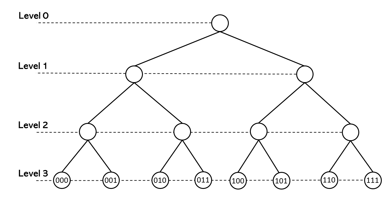
Figure 1: The rooted tree associated with the group $\mathbb{Z}_{2}/2^{3}\mathbb{Z}_{2}$. The elements of $\mathbb{Z}_{2}/2^{3}\mathbb{Z}_{2}$ have the form $i=i_{0}+i_{1}2+i_{2}2^{2}$,$\;i_{0}$, $i_{1}$, $i_{2}\in\{0,1\}$. The distance satisfies $-\log_{2}\left|i-j\right|_{2}=$level of the first common ancestor of $i$, $j$.

4.2 The Haar measure

Since $(\mathbb{Z}_{p},+)$ is a compact topological group, there exists a Haar measure $dx$, which is invariant under translations, i.e., $d(x+a)=dx$, [36]. If we normalize this measure by the condition $\int_{\mathbb{Z}_{p}}dx=1$, then $dx$ is unique. It follows immediately that

$${\textstyle\int\limits_{B_{-r}(a)}}dx={\textstyle\int\limits_{a+p^{r}\mathbb{Z}_{p}}}dx=p^{-r}{\textstyle\int\limits_{\mathbb{Z}_{p}}}dy=p^{-r}\text{, }r\in\mathbb{N}\text{.}$$

In a few occasions, we use the two-dimensional Haar measure $dxdy$ of the additive group $(\mathbb{Z}_{p}\times\mathbb{Z}_{p},+)$ normalize this measure by the condition $\int_{\mathbb{Z}_{p}}\int_{\mathbb{Z}_{p}}dxdy=1$. For a a quick review of the integration in the $p$-adic framework, the reader may consult [33] and the references therein.

4.3 The Bruhat-Schwartz space in the unit ball

A real-valued function $\varphi$ defined on $\mathbb{Z}_{p}$ is called Bruhat-Schwartz function (or a test function) if for any $x\in\mathbb{Z}_{p}$ there exist an integer $l\in\mathbb{N}$ such that

$$\varphi(x+x^{\prime})=\varphi(x)\text{ for any }x^{\prime}\in B_{l}.$$ (4.2)

The $\mathbb{R}$-vector space of Bruhat-Schwartz functions supported in the unit ball is denoted by $\mathcal{D}(\mathbb{Z}_{p})$. For $\varphi\in\mathcal{D}(\mathbb{Z}_{p})$, the largest number $l=l(\varphi)$ satisfying (4.2) is called the exponent of local constancy (or the parameter of constancy) of $\varphi$. A function $\varphi$ in $\mathcal{D}(\mathbb{Z}_{p})$ can be written as

$$\varphi\left(x\right)={\displaystyle\sum\limits_{j=1}^{M}}\varphi\left(\widetilde{x}_{j}\right)\Omega\left(p^{-r_{j}}\left|x-\widetilde{x}_{j}\right|_{p}\right),$$

where the $\widetilde{x}_{j}$, $j=1,\ldots,M$, are points in $\mathbb{Z}_{p}$, the $r_{j}$, $j=1,\ldots,M$, are non-negative integers, and $\Omega\left(p^{r_{j}}\left|x-\widetilde{x}_{j}\right|_{p}\right)$ denotes the characteristic function of the ball $B_{-r_{j}}(\widetilde{x}_{j})=\widetilde{x}_{j}+p^{r_{j}}\mathbb{Z}_{p}$.

We denote by $\mathcal{D}^{l}(\mathbb{Z}_{p})$ the $\mathbb{R}$-vector space of all test functions of the form

$$\varphi\left(x\right)={\textstyle\sum\limits_{i\in G_{l}}}\varphi\left(i\right)\Omega\left(p^{l}\left|x-i\right|_{p}\right)\text{, \ }\varphi\left(i\right)\in\mathbb{R}\text{,}$$

where $i=i_{0}+i_{1}p+\ldots+i_{l-1}p^{l-1}\in G_{l}=\mathbb{Z}_{p}/p^{l}\mathbb{Z}_{p}$, $l\geq 1$. Notice that $\varphi$ is supported on $\mathbb{Z}_{p}$ and that $\mathcal{D}(\mathbb{Z}_{p})=\cup_{l\in\mathbb{N}}\mathcal{D}^{l}(\mathbb{Z}_{p})$.

The space $\mathcal{D}^{l}(\mathbb{Z}_{p})$ is a finite-dimensional vector space spanned by the basis $\left\{\Omega\left(p^{l}\left|x-i\right|_{p}\right)\right\}_{i\in G_{l}}$. By identifying $\varphi\in\mathcal{D}^{l}(\mathbb{Z}_{p})$ with the column vector $\left[\varphi\left(i\right)\right]_{i\in G_{l}}\in\mathbb{R}^{\#G_{l}}$, we get that $\mathcal{D}^{l}(\mathbb{Z}_{p})$ is isomorphic to $\mathbb{R}^{\#G_{l}}$ endowed with the norm

$$\left\|\left[\varphi\left(i\right)\right]_{i\in G_{l}^{N}}\right\|=\max_{i\in G_{l}}\left|\varphi\left(i\right)\right|.$$

Furthermore,

$$\mathcal{D}^{l}\hookrightarrow\mathcal{D}^{l+1}\hookrightarrow\mathcal{D}(\mathbb{Z}_{p}),$$

where $\hookrightarrow$ denotes a continuous embedding.

4.4 The $p$-adic version and discrete version of the Wilson-Cowan models

The $p$-adic Wilson-Cowan model is obtained by taking $\mathcal{G}=\mathbb{Z}_{p}$ and $d\mu=dx$ in (2.10).

On the other hand, $\left\|f\right\|_{1}\leq\left\|f\right\|_{\infty}$, and

$$L^{1}(\mathbb{Z}_{p})\supseteq L^{\infty}(\mathbb{Z}_{p})\supseteq\mathcal{C}(\mathbb{Z}_{p})\supseteq\mathcal{D}(\mathbb{Z}_{p}),$$

where $\mathcal{C}(\mathbb{Z}_{p})$ denotes the $\mathbb{R}$-space of continuous functions on $\mathbb{Z}_{p}$ endowed with the norm $\left\|\cdot\right\|_{\infty}$. Futhermore, $\mathcal{D}(\mathbb{Z}_{p})$ is dense in $L^{1}(\mathbb{Z}_{p})$, [30, Proposition 4.3.3], and consequently, it is also dense in $L^{\infty}(\mathbb{Z}_{p})$ and $\mathcal{C}(\mathbb{Z}_{p})$.

For the sake of simplicity, we assume that $w_{EE}$, $w_{IE}$, $w_{EI}$, $w_{II}\in\mathcal{C}(\mathbb{Z}_{p})$, and $h_{E}\left(x,t\right)$, $h_{I}\left(x,t\right)\in\mathcal{C}(\left[0,\infty\right],\mathcal{C}(\mathbb{Z}_{p}))$. Theorem 2.5 is still valid under these hypotheses. We use the theory of approximation of evolution equations to construct good discretizations of the $p$-adic Wilson-Cowan system, see, e.g., [5, Section 5.4].

This theory requires the following hypotheses.

(A). (a) $\mathcal{X}=\left(\mathcal{C}(\mathbb{Z}_{p})\times\mathcal{C}(\mathbb{Z}_{p})\right)$, $\mathcal{X}_{l}=\left(\mathcal{D}^{l}(\mathbb{Z}_{p})\times\mathcal{D}^{l}(\mathbb{Z}_{p})\right)$, $l\geq 1$, endowed with the norm $\left\|f\right\|=\left\|\left(f_{1},f_{2}\right)\right\|=\max\left\{\left\|\left(f_{1}\right)\right\|_{\infty},\left\|\left(f_{2}\right)\right\|_{\infty}\right\}$ are Banach spaces. It is relevant to mention that $\mathcal{X}_{l}$ is a subspace of $\mathcal{X}$, and that $\mathcal{X}_{l}$ is a subspace of $\mathcal{X}_{l+1}$.

(b) The operator

$$\begin{array}[c]{cccc}\boldsymbol{P}_{l}:&\mathcal{X}&\rightarrow&\mathcal{X}_{l}\\ &&&\\ &f\left(x\right)&\rightarrow&\left(\boldsymbol{P}_{l}f\right)\left(x\right)={\textstyle\sum\limits_{i\in G_{l}}}f\left(i\right)\Omega\left(p^{l}\left|x-i\right|_{p}\right)\end{array}$$

is linear and bounded, i.e., $\boldsymbol{P}_{l}\in\mathbb{B}(\mathcal{X},\mathcal{X}_{l})$, and $\left\|\boldsymbol{P}_{l}f\right\|\leq\left\|f\right\|$, for every $f\in\mathcal{X}$.

(c) We set $\boldsymbol{1}_{l}:\mathcal{X}_{l}\rightarrow\mathcal{X}$ to be the identity operator. Then $\boldsymbol{1}_{l}\in\mathbb{B}(\mathcal{X}_{l},\mathcal{X})$, and $\left\|\boldsymbol{1}_{l}f\right\|=\left\|f\right\|$, for every $f\in\mathcal{X}_{l}$.

(d) $\boldsymbol{P}_{l}\boldsymbol{1}_{l}f=f$, for $l\geq 1$, $f\in\mathcal{X}_{l}$.

(B), (C). The Wilson-Cowan system, see (2.10), involves the operator $\frac{1}{\tau}\mathbf{1}$, where $\mathbf{1}\in\mathbb{B}(\mathcal{X},\mathcal{X})$ is the identity operator. As approximation, we use $\mathbf{1}\in\mathbb{B}(\mathcal{X}_{l},\mathcal{X}_{l})$, for every $l\geq 1$. Furthermore,

$$\lim_{l\rightarrow\infty}\left\|\mathbf{P}_{l}f-f\right\|=0,$$

see [37, Lemma 1].

(D). For $t\in\left(0,\infty\right)$, $\frac{1}{\tau}\boldsymbol{H}(s,f):\left[0,t\right]\times\mathcal{X}\rightarrow\mathcal{X}$ is a continuous and such that for some $L<\infty$,

$$\left\|\frac{1}{\tau}\boldsymbol{H}(s,f)-\frac{1}{\tau}\boldsymbol{H}(s,g)\right\|\leq L\left\|f-g\right\|\text{,}$$

for $0\leq s\leq t$, $f$, $g\in\mathcal{X}$. This assertion is a consequence of the fact that $\boldsymbol{H}:\mathcal{X}\rightarrow\mathcal{X}$ is a well-defined globally Lipschitz, see Lemma 2.3.

We use the notation $E\left(t\right)=E\left(\cdot,t\right)$, $I\left(t\right)=I\left(\cdot,t\right)\in\mathcal{C}^{1}(\left[0,T\right),\mathcal{X})$, and for the approximations $E_{l}\left(t\right)=E_{l}\left(\cdot,t\right)$, $I_{l}\left(t\right)=I_{l}\left(\cdot,t\right)\in\mathcal{C}^{1}(\left[0,T\right),\mathcal{X})$. The space discretization of the $p$-adic Wilson-Cowan system (2.10) is

$$\left\{\begin{array}[c]{l}\frac{\partial}{\partial t}\left[\begin{array}[c]{c}E_{l}\left(t\right)\\ I_{l}\left(t\right)\end{array}\right]+\frac{1}{\tau}\left[\begin{array}[c]{c}E_{l}\left(t\right)\\ I_{l}\left(t\right)\end{array}\right]=\frac{1}{\tau}\boldsymbol{P}_{l}\left(\boldsymbol{H}(\left[\begin{array}[c]{c}E_{l}\left(t\right)\\ I_{l}\left(t\right)\end{array}\right])\right),\\ \\ \left[\begin{array}[c]{c}E_{l}\left(0\right)\\ I_{l}\left(0\right)\end{array}\right]=\boldsymbol{P}_{l}\left(\left[\begin{array}[c]{c}E_{0}\left(x\right)\\ I_{0}\left(x\right)\end{array}\right]\right)\in\mathcal{X}_{l}.\end{array}\right.$$ (4.3)

The next step is to obtain an explicit expression for the space discretization given in (4.3). We need the following formulae.

Remark 4.1

Take

$$w(x)={\displaystyle\sum\limits_{j\in G_{l}}}w\left(j\right)\Omega\left(p^{l}\left|x-j\right|_{p}\right)\text{, }\phi(y)={\displaystyle\sum\limits_{i\in G_{l}}}\phi\left(i\right)\Omega\left(p^{l}\left|y-i\right|_{p}\right)\in\mathcal{D}^{l}(\mathbb{Z}_{p}).$$

Then

$$\left(w\ast\phi\right)\left(x\right)={\displaystyle\int\limits_{\mathbb{Z}_{p}}}w\left(x-y\right)\phi\left(y\right)dy=\\ {\displaystyle\sum\limits_{k\in G_{l}}}\left\{{\displaystyle\sum\limits_{i\in G_{l}}}w\left(k-i\right)\phi\left(i\right)\right\}\Omega\left(p^{l}\left|x-k\right|_{p}\right)\in\mathcal{D}^{l}(\mathbb{Z}_{p}).$$

Indeed,

$$\left(w\ast\phi\right)\left(x\right)={\displaystyle\sum\limits_{j\in G_{l}}}\text{ }{\displaystyle\sum\limits_{i\in G_{l}}}w\left(j\right)\phi\left(i\right){\displaystyle\int\limits_{\mathbb{Z}_{p}}}\Omega\left(p^{l}\left|x-y-j\right|_{p}\right)\Omega\left(p^{l}\left|y-i\right|_{p}\right)dy.$$

Changing variables as $z=y-i$, $dz=dx$, in the integral,

$$\left(w\ast\phi\right)\left(x\right) ={\displaystyle\sum\limits_{j\in G_{l}}}\text{ }{\displaystyle\sum\limits_{i\in G_{l}}}w\left(j\right)\phi\left(i\right){\displaystyle\int\limits_{\mathbb{Z}_{p}}}\Omega\left(p^{l}\left|x-z-\left(i+j\right)\right|_{p}\right)\Omega\left(p^{l}\left|z\right|_{p}\right)dz$$

$$={\displaystyle\sum\limits_{j\in G_{l}}}\text{ }{\displaystyle\sum\limits_{i\in G_{l}}}w\left(j\right)\phi\left(i\right){\displaystyle\int\limits_{p^{l}\mathbb{Z}_{p}}}\Omega\left(p^{l}\left|x-z-\left(i+j\right)\right|_{p}\right)dz.$$

Now, by taking $k=i+j$, and using the fact that $G_{l}$ is an additive group,

$$\left(w\ast\phi\right)\left(x\right) ={\displaystyle\sum\limits_{k\in G_{l}}}\text{ }{\displaystyle\sum\limits_{i\in G_{l}}}w\left(k-i\right)\phi\left(i\right){\displaystyle\int\limits_{p^{l}\mathbb{Z}_{p}}}\Omega\left(p^{l}\left|x-z-k\right|_{p}\right)dz$$

$$={\displaystyle\sum\limits_{k\in G_{l}}}\left\{{\displaystyle\sum\limits_{i\in G_{l}}}w\left(k-i\right)\phi\left(i\right)\right\}\Omega\left(p^{l}\left|x-k\right|_{p}\right).$$

Remark 4.2

Take $S:\mathbb{R\rightarrow}\mathbb{R}$. Then

$$S\left({\displaystyle\sum\limits_{i\in G_{l}}}\phi\left(i\right)\Omega\left(p^{l}\left|y-i\right|_{p}\right)\right)={\displaystyle\sum\limits_{i\in G_{l}}}S\left(\phi\left(i\right)\right)\Omega\left(p^{l}\left|y-i\right|_{p}\right).$$

This formula follows from the fact that the supports of the functions $\Omega\left(p^{l}\left|y-i\right|_{p}\right)$, $i\in G_{l}$, are disjoint.

The space discretization of the integro-differential equation in (4.3) is obtained by computing the term $\boldsymbol{P}_{l}\left(\boldsymbol{H}(\left[\begin{array}[c]{c}E_{l}\left(t\right)\\ I_{l}\left(t\right)\end{array}\right])\right)$ using Remarks 4.1-4.2. By using the notation

$$w_{l}^{AB}=\left[w_{i}^{AB}\right]_{i\in G_{l}},\ w_{i}^{AB}=w_{AB}\left(i\right)\text{, for }A,B\in\left\{E,I\right\},$$

$$E_{l}(t)=\left[E_{i}\left(t\right)\right]_{i\in G_{l}}\text{, }E_{i}\left(t\right)=E\left(i,t\right)\text{, and }I_{l}(t)=\left[I_{i}\left(t\right)\right]_{i\in G_{l}}\text{, }I_{i}\left(t\right)=I\left(i,t\right),$$

$$h_{l}^{A}\left(t\right)=\left[h_{i}^{A}\left(t\right)\right]_{i\in G_{l}}\text{, }h_{i}^{A}\left(t\right)=h_{A}\left(i,t\right)\text{, for }A\in\left\{E,I\right\},$$

and for $\phi_{l}=\left[\phi_{i}\right]_{i\in G_{l}}$, $\theta_{l}=\left[\theta_{i}\right]_{i\in G_{l}}$,

$$\phi_{l}\ast\theta_{l}=\left[\text{ }{\displaystyle\sum\limits_{k\in G_{l}}}\phi_{i-k}\theta_{k}\right]_{i\in G_{l}}.$$

With this notation, the announced discretization takes the following form:

$$\left\{\begin{array}[c]{cc}\tau\frac{\partial E_{l}(t)}{\partial t}=&-E_{l}(t)+S_{E}\left(w_{l}^{EE}\ast E_{l}(t)-w_{l}^{EI}\ast I_{l}(t)+h_{l}^{E}\left(t\right)\right)\\ &\\ \tau\frac{\partial I_{l}(t)}{\partial t}=&-I_{l}(t)+S_{I}\left(w_{l}^{IE}\ast E_{l}(t)-w_{l}^{II}(x)\ast I_{l}(t)+h_{l}^{I}\left(t\right)\right).\end{array}\right.$$

Theorem 4.3

Take $r_{I}=$ $r_{E}=0$, $\left[\begin{array}[c]{c}E_{0}\left(x\right)\\ I_{0}\left(x\right)\end{array}\right]\in\mathcal{X}$, and $T\in\left(0,\infty\right)$. Let $\left[\begin{array}[c]{c}E\left(t\right)\\ I\left(t\right)\end{array}\right]\in$ $\mathcal{C}^{1}(\left[0,T_{0}\right),\mathcal{X})$ be the solution (2.11)-(2.12) given in Theorem 2.5. Let $\left[\begin{array}[c]{c}E_{l}\left(t\right)\\ I_{l}\left(t\right)\end{array}\right]$ be the solution of the Cauchy problem (4.3). Then

$$\lim_{l\rightarrow\infty}\sup_{0\leq t\leq T}\left\|\left[\begin{array}[c]{c}E_{l}\left(t\right)\\ I_{l}\left(t\right)\end{array}\right]-\left[\begin{array}[c]{c}E\left(t\right)\\ I\left(t\right)\end{array}\right]\right\|=0.$$

Proof. We first notice that Theorem 2.5 is valid for the Cauchy problem (4.3), more precisely, this problem has a unique solution $\left[\begin{array}[c]{c}E_{l}\left(t\right)\\ I_{l}\left(t\right)\end{array}\right]$ in $\mathcal{C}^{1}(\left[0,T_{0}\right),\mathcal{X}_{l})$ satisfying properties akin to the ones stated in Theorem 2.5. Since $\mathcal{X}_{l}$ is a subspace of $\mathcal{X}$, by applying Theorem 2.5 to the Cauchy problem (4.3), we get the existence of a unique solution $\left[\begin{array}[c]{c}E_{l}\left(t\right)\\ I_{l}\left(t\right)\end{array}\right]$ in $\mathcal{C}^{1}(\left[0,T_{0}\right),\mathcal{X})$ satisfying the properties announced in Theorem 2.5. To show that the solution $\left[\begin{array}[c]{c}E_{l}\left(t\right)\\ I_{l}\left(t\right)\end{array}\right]$ belongs to $\mathcal{C}(\left[0,T_{0}\right),\mathcal{X}_{l})$, we use [5, Theorem 5.2.2]. For similar reasoning, the reader may consult Remark 2, and the proof of Theorem 1 in [27]. The proof of the the theorem follows from hypotheses A, B, C, and D by [5, Theorem 5.4.7]. For similar reasoning, the reader may consult the proof of Theorem 4 in [27].   

5 Numerical simulations

Remark 5.1

We use heat maps to visualize approximations of the solutions of $p$-adic discrete Wilson-Cowan Equations (4.3). The vertical axis gives the position, which is a truncated $p$-adic number. These numbers correspond to a rooted tree’s vertices at the top level, i.e., $G_{l}$; see Figure 1. By convenience, we include a representation of this tree. The heat maps’ colors represent the solutions’ values in a particular neuron. For instance, take $p=2$, $l=4$, and

$$\phi(x)=\Omega(2^{4}|x|_{2})-\Omega(2^{4}|x-2|_{2})+\Omega(2^{4}|x-1|_{2})+\Omega(2^{4}|x-7|_{2}).$$ (5.1)

The corresponding heat map is shown in Figure 2. If the function depends on two variables, say $\phi(x,t)$, where $x\in\mathbb{Z}_{p}$ and $t\in\mathbb{R}$, the corresponding heat map color represents the value of $\phi(x,t)$ at time $t$ and neuron $x$.

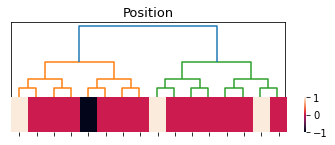
Figure 2: Heat map of the function $\phi(x)$, see (5.1). Here, $\phi(0)=\phi(1)=\phi(7)=1$ is white, $\phi(2)=-1$ is black, and $\phi(x)=0$ is red for $x\neq 0,1,7,2$.

We take $\tau=10$, $r_{I}=r_{E}=1$, $p=3$, $l=6$,

$$w_{AB}(x)=b_{AB}\exp(\sigma_{AB})-b_{AB}\exp(\sigma_{AB}|x|_{p})\text{, for }A,B\in\left\{E,I\right\},$$

and

$$S_{A}(z)=\frac{1}{1+\exp(-v_{A}(z-\theta_{A}))}-\frac{1}{1+\exp(v_{A}\theta_{A})}\text{, for }z\in\mathbb{R},\text{ }A\in\left\{E,I\right\}.$$

The kernel $w_{AB}(x)$ is a decresing function of $|x|_{p}$. Thus, near neurons interact strongly. $S_{A}(z)$ is a sigmoid function satisfying $S_{A}(0)=0$.

5.1 Numerical simulation 1

The purpose of this experiment is to show the response of the $p$-adic Wilson-Cowan network to a short pulse, and a constant stimulus. See Figure 3, 4, 5. Our results are consistent with the results obtained by Cowan and Wilson in [2, Section 2.2.1-Section 2.2.5]. The pulses are

$$h_{E}(x,t)=3.7\Omega(p^{2}|x-4|_{p})1_{[0,\delta]}(t)\text{, for }x\in\mathbb{Z}_{p}\text{, }t\in\left[0,\delta\right]\text{,}$$ (5.2)

$$h_{I}(x,t)=Q\Omega(|x-4|_{p})1_{[0,\delta]}(t)\text{, for }x\in\mathbb{Z}_{p}\text{, }t\in\left[0,\delta\right]\text{,}$$ (5.3)

where $1_{[0,\delta]}(t)$ is the characteristic function of the time interval $\left[0,\delta\right]$, $\delta>0$. We use the following parameters: $v_{E}=2.75$, $v_{I}=0.3$, $b_{EE}=1.5$, $\sigma_{EE}=4$, $b_{II}=1.8$, $\sigma_{II}=3$, $\theta_{E}=9$, $\theta_{I}=17$, $b_{IE}=1.35$, $\sigma_{IE}=6$, $b_{EI}=1.35$, $\sigma_{EI}=6$.

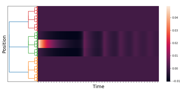
Figure 3: An approximation of $E(x,t)$. We take $Q=0$, $\delta=5$. The time axis goes from $0$ to $100$. The figure shows the response of the network to a brief localized stimulus (the  pulse given in (5.2)). The response is also a pulse. This result is consistent with the numerical results in [1, Section 2.2.1, Figure 3].

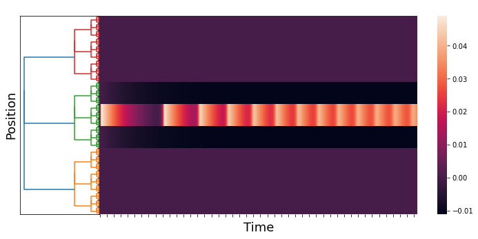
Figure 4: An approximation of $E(x,t)$. We take $Q=0$, $\delta=100$. The time axis goes from $0$ to $100$. The figure shows the response of the network to a maintained stimulus (see (5.2)). The response is a pulse train. This result is consistent with the numerical results in [1, Section 2.2.5, Figure 7].

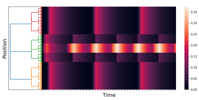
Figure 5: An approximation of $E(x,t)$. We take $Q=-30$, $\delta=100$. The time axis goes from $0$ to $100$. The figure shows the response of the network to a maintained stimulus (see (5.2)-(5.3)). The response is a pulse train in space and time. This result is consistent with the numerical results in [1, Section 2.2.7, Figure 9].

5.2 Numerical simulation  2

In [2, Section 3.3.1], Wilson and Cowan applied their model to the spatial hysteresis in the one-dimensional tissue model. In this experiment, a human subject was exposed to a binocular stimulus. The authors used sharply peaked Gaussian distributions to model the stimuli. The two stimuli were symmetrically moved apart by a small increment and re-summed, and the network response was allowed to reach equilibrium.

Initially, the two peaks (stimuli) were very closed; the network response consisted of a single pulse (peak), see [2, Section 3.3.1, Figure 13-A]. Then, the peaks separated from each other (i.e., the disparity between the two stimuli increased). The network response was a pulse in the middle of the binocular stimulus until a critical disparity was reached. At this stimulus disparity, the single pulse (peak) decayed rapidly to zero, and twin response pulses formed at the locations of the now rather widely separated stimuli, see [2, Section 3.3.1, Figure 13-B].

Following this, the stimuli were gradually moved together again in the same form until they essentially consisted of one peak. But the network response consisted of two pulses, see [2, Section 3.3.1, Figure 13-C].

The classical Wilson-Cowan model and our $p$-adic version can predict the results of this experiment. We use the function

$$\widetilde{h}_{E}(x,t)=e^{-(30(0.5-\mathfrak{m}(x))-0.5t)^{2}}+e^{-(30(0.5-\mathfrak{m}(x))+0.5t)^{2}}$$ (5.4)

to model the stimuli in the case where the peaks do not move together, and

$$h_{E}(x,t)=\widetilde{h}_{E}(x,t)1_{[0,18]}(t)+\widetilde{h}_{E}(x,36-t)1_{[18,36]}(t)$$ (5.5)

to model the stimuli in the case where the peaks gradually move together. The function $\mathfrak{m}:\mathbb{Z}_{p}\rightarrow\mathbb{R}$ is the Monna map, see [38].

Figure 6 shows the stimuli (see (5.4)) and the network response when the stimuli peaks are gradually separated. The network response begins with a single pulse. When a critical disparity threshold is reached, the response becomes a twin pulse. Which is the prediction of the classical Wilson-Cowan model, see [2, Section 3.3.1, Figures 13-A, 13-B.].

Figure 7 depicts the stimuli and the network response in the instance where the stimuli peaks gradually split, and finally move together. The network response at the end of the experiment consists of twin pulses. This finding is consistent with that of the classical Wilson-Cowan model, [2, Section 3.3.1, Figure 13-C].

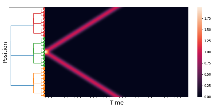
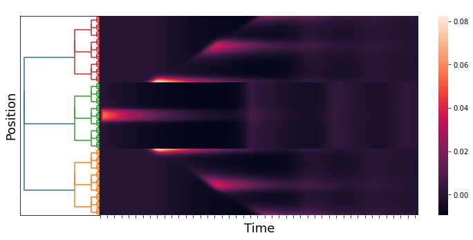
Figure 6: An approximation of $\widetilde{h}_{E}(x,t)$ and $E(x,t)$. We take $h_{I}(x,t)\equiv 0$, $p=3$, $l=6$, the kernels $w_{AB}$ are as in the Simulation 1, and the $h_{E}(x,t)$ as in (5.4). The time axis goes from $0$ to $60$. The first figure is the stimuli and the second figure is the response of the network.

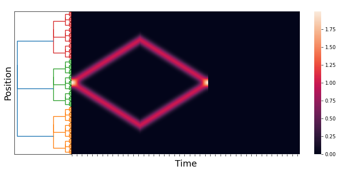
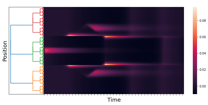
Figure 7: An approximation of $h_{E}(x,t)$ and $E(x,t)$. We take $h_{I}(x,t)\equiv 0$, $p=3$, $l=6$, the kernels $w_{AB}$ are as in the Simulation 1, and the $h_{E}(x,t)$ as in (5.5). The time axis goes from $0$ to $60$. The first figure is the stimuli and the second figure is the response of the network.

6 $p$-Adic kernels and connection matrices

There have been significant theoretical and experimental developments in comprehending the wiring diagrams (connection matrices) of the cerebral cortex of invertebrates and mammals over the last thirty years, see, for example, [6]-[19] and the references therein. The topology of cortical neural networks is described by connection matrices. Building dynamic models from experimental data recorded in connection matrices is a very relevant problem.

We argue that our $p$-adic Wilson-Cowan model provides meaningful dynamics on networks whose topology comes from a connection matrix. Figure 8 depicts the connection matrix of the cat cortex, see, e.g., [7]-[14], and the matrix of the kernel $w_{EE}$ used in the Simulation 1. The $p$-adic methods are relevant only if the connection matrices can be very well approximated for matrices coming from discretizations of $p$-adic kernels. This is an open problem. Here, we show that such an approximation is feasible for the cat cortex connection matrix.

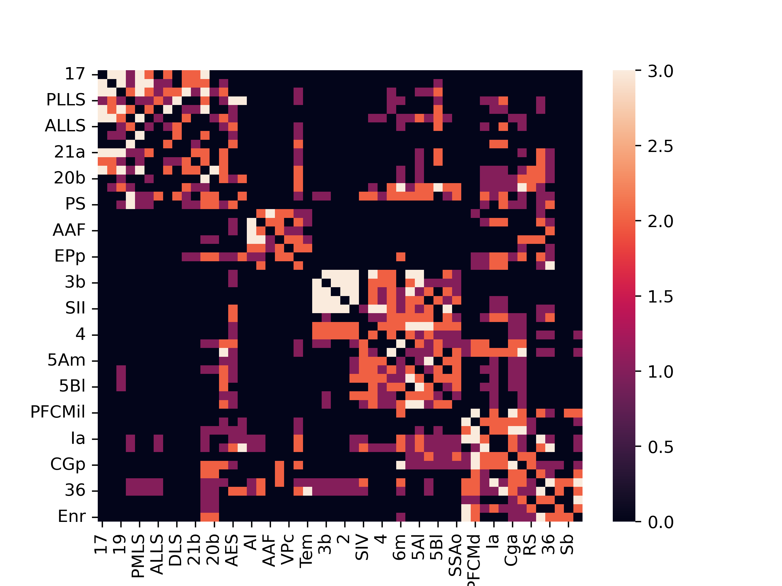
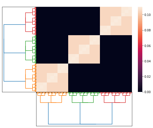
Figure 8: The left matrix is the connection matrix of the cat cortex. The right matrix corresponds to a discretization of the kernel $w_{EE}$ use in the simulation 1.

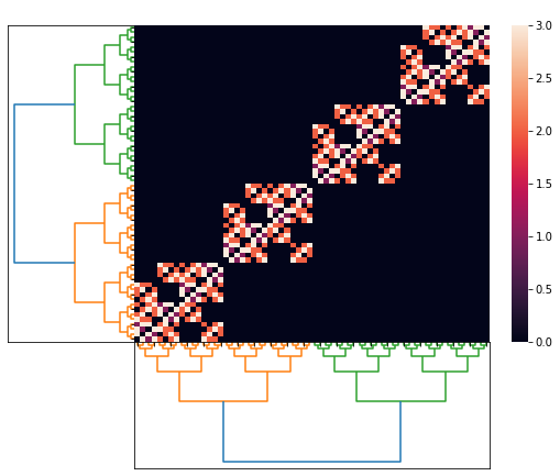
Figure 9: Three $p$-adic approximations for the connection matrix of the cat cortex. We take $p=2$, $l=6$. The first approximation uses $r=0$, the second $r=3$, and the last $r=5$.

By using the above procedure, we replace the excitatory-excitatory relation term $w_{EE}\ast E$ by $\int_{\mathbb{Z}_{p}}K_{r}(x,y)E(y)dy$ but keep the other kernels as in Simulation 1. For the stimuli we use $h_{E}=3.5\Omega(p^{2}|x-1|_{p})$, with $p=2$, $l=6$, and $h_{I}(x)=-30$. In the Figure 9, we show three different approximations for the cat cortex connection matrix using $p$-adic kernels. The black area in the right matrix in Figure 9 (which correspond to zero entries) comes from the process of adjusting the size of origin matrix to $2^{6}\times 2^{6}$.

The corresponding $p$-adic network responses are shown in Figure 10 for different values of $r$. In the case, $r=0$, the interaction between the neurons is short-range, while in the case $r=5$, there is long-range interaction. The response in the case $r=0$ is similar to the one presented in Simulation 1; see Figure 5. When the connection matrix gets close to the cat cortex matrix (see Figure 9), which is when the matrix allows more long-range connections, the response of the network presents more complex patterns (see Figure 10).

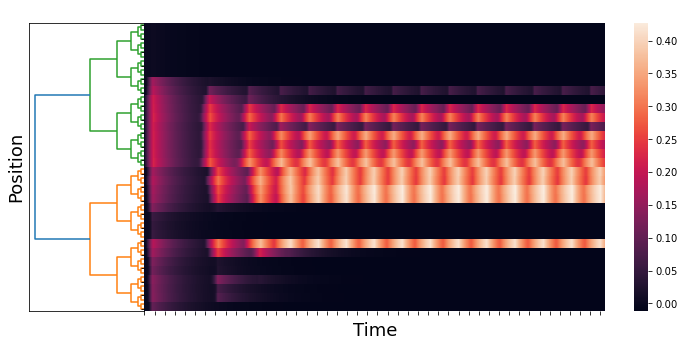
Figure 10: We use $p=2$, $l=6$, and time axis goes from $0$ to $150$. The left image uses $r=0$, the right one uses $r=3$, and the central one uses $r=5$.

7 Final Discussion

The Wilson–Cowan model describes interactions between populations of excitatory and inhibitory neurons. This model constitutes a relevant mathematical tool for understanding cortical tissue’s functionality. On the other hand, in the last twenty-five years, there has been tremendous experimental development in understanding the cerebral cortex’s neuronal wiring in invertebrates and mammalians. Employing different experimental techniques, the wiring patterns can be described by connection matrices. A such matrix is just an adjacency matrix of a directed graph whose nodes represent neurons, groups of neurons, or portions of the cerebral cortex. The oriented edges represent the strength of the connections between two groups of neurons. This work explores the interplay between the classical Wilson-Cowan model and the connections matrices.

Nowadays, it is widely accepted that the networks in the cerebral cortex of mammalians have the small-world property, which means a non-negligible interaction exists between any two groups of neurons in the network. The classical Wilson-Cowan model is not compatible with the small-world property. We show that the original Wilson-Cowan model can be formulated on any topological group, and the Cauchy problem for the underlying equations of the model is well-posed. We gave an argument showing that the small-world property requires that the group be compact, and consequently, the classical model should be discarded. In practical terms, the classical Wilson-Cowan model cannot incorporate the experimental information contained in the connection matrices. We proposed a $p$-adic Wilson-Cowan model, where the neurons are organized in an infinite rooted tree. We present numerical experiments showing that this model can explain several phenomena like the classical model. The new model can incorporate the experimental information coming from the connection matrices.

References

- [1] Wilson H. R., Cowan J. D. (1972). Excitatory and inhibitory interactions in localized populations of model neurons, Biophys J. 12(1), 1-24.
- [2] Wilson H. R., Cowan J. D. A. (1973). Mathematical theory of the functional dynamics of cortical and thalamic nervous tissue, Kybernetik 13(2), 55-80.
- [3] Coobes Stephen, baim Graben Peter, Potthast Roland, and Wright James, Editors. (2014). Neural fields. Theory and applications. Springer, Heidelberg.
- [4] Cazenave Thierry, Haraux Alain. (1998). An introduction to semilinear evolution equations. Oxford University Press.
- [5] Miklavčič Milan. (1998). Applied functional analysis and partial differential equations. World Scientific Publishing Co., Inc., River Edge, NJ,
- [6] Sporns O., Tononi G., Edelman G. M. (2000). Theoretical neuroanatomy: relating anatomical and functional connectivity in graphs and cortical connection matrices, Cerebral Cortex, 10( 2), 127–14.
- [7] Scannell, J. W., Burns, G. A., Hilgetag, C. C., O’Neil, M. A. , Young, M. P. (1999). The connectional organization of the cortico-thalamic system of the cat, Cerebral Cortex, 9(3), 277–299.
- [8] Sporns O. (2006). Small-world connectivity, motif composition, and complexity of fractal neuronal connections, Biosystems, 85(1), 55-64.
- [9] Sporns O, Honey C. J. (2006). Small worlds inside big brains, Proc Natl Acad Sci USA. 103(51):19219-20.
- [10] Hilgetag C. C., Goulas A. (2016). Is the brain really a small-world network? Brain Struct Funct. 221(4), 2361-6.
- [11] Muldoon S. F., Bridgeford E. W., Bassett D. S. (2016). Small-World Propensity and Weighted Brain Networks, Sci Rep. 6, 22057.
- [12] Bassett D. S., Bullmore E. T. (2017). Small-World Brain Networks Revisited, Neuroscientist, 23(5), 499-516.
- [13] Akiki T. J., Abdallah C. G. (2019). Determining the Hierarchical Architecture of the Human Brain Using Subject-Level Clustering of Functional Networks, Sci Rep 9, 19290.
- [14] Scannell J. W., Blakemore C., Young M. P.(1995). Analysis of connectivity in the cat cerebral cortex, J. Neurosci. 15(2), 1463-83.
- [15] Fornito Alex, Zalesky Andrew, Bullmore Edward T. Editors. (2016). Connectivity Matrices and Brain Graphs in Fundamentals of Brain Network Analysis. Academic Press. Pages 89-113.
- [16] Sporns Olaf. (2016). Networks of the Brain. Penguin Random House LLC, 2016.
- [17] Swanson L. W., Hahn J. D., Sporns O. (2017). Organizing principles for the cerebral cortex network of commissural and association connections, Proc Natl Acad Sci U S A, 114(45), E9692-E9701.
- [18] Demirtaş M., Burt J. B., Helmer M., Ji J. L., Adkinson B. D., Glasser M. F., Van Essen D. C., Sotiropoulos S. N., Anticevic A., Murray J. D. (2019). Hierarchical Heterogeneity across Human Cortex Shapes Large-Scale Neural Dynamics, Neuron, 101, 1181–1194.
- [19] Škoch A., Rehák Bučková B., Mareš J., Tintěra J., Sanda P., Jajcay L., Horáček J., Španiel F., Hlinka J. (2022). Human brain structural connectivity matrices-ready for modeling, Sci Data, 9, 486.
- [20] Avetisov V. A., Bikulov A. Kh., Osipov V. A. (2003). p-Adic description of characteristic relaxation in complex systems, J. Phys. A 36 (15), 4239–4246.
- [21] Avetisov V. A., Bikulov A. H., Kozyrev S.V., Osipov V. A. (2002). p-Adic models of ultrametric diffusion constrained by hierarchical energy landscapes, J. Phys. A 35 (2), 177–189.
- [22] Parisi G., Sourlas N. (2000). p-Adic numbers and replica symmetry breaking, Eur. Phys. J. B 14, 535–542.
- [23] Khrennikov Andrei, Kozyrev Sergei, Zúñiga-Galindo W. A. (2018). Ultrametric Equations and its Applications. Encyclopedia of Mathematics and its Applications 168. Cambridge University Press.
- [24] Zúñiga-Galindo W. A. (2022). Eigen’s paradox and the quasispecies model in a non-Archimedean framework, Physica A: Statistical Mechanics and its Applications, 602 , Paper No. 127648, 18 pp.
- [25] Zúñiga-Galindo W. A. (2022). Ultrametric diffusion, rugged energy landscapes, and transition networks, Physica A: Statistical Mechanics and its Applications, 597 , Paper No. 127221, 19 pp.
- [26] Zúñiga-Galindo W. A. (2020). Reaction-diffusion equations on complex networks and Turing patterns, via p-adic analysis, J. Math. Anal. Appl. 491(1), 124239, 39 pp.
- [27] Zambrano-Luna B.A., Zuniga-Galindo W.A. (2023). -Adic cellular neural networks, J. Nonlinear Math. Phys. 30(1), 34–70.
- [28] Zambrano-Luna B. A., Zúñiga-Galindo W. A. (2023). -Adic cellular neural networks: Applications to image processing, Physica D: Nonlinear Phenomena, 446 , Paper No. 133668, 11 pp.
- [29] Vladimirov V. S., Volovich I. V., Zelenov E. I. (1994). -Adic analysis and mathematical physics. Singapore, World Scientific.
- [30] Albeverio S., Khrennikov A. Yu., Shelkovich V. M. (2010). Theory of -adicdistributions: linear and nonlinear models. Cambridge University Press.
- [31] Kochubei Anatoly N. (2001). Pseudo-differential equations and stochastics over non-Archimedean fields. New York, Marcel Dekker.
- [32] Taibleson M. H. (1975). Fourier analysis on local fields. Princeton University Press.
- [33] Bocardo-Gaspar Miriam, García-Compeán H., Zúñiga-Galindo W. A. (2019). Regularization of p-adic string amplitudes, and multivariate local zeta functions, Lett. Math. Phys. 109(5), 1167–1204.
- [34] Koblitz Neal. (1984). -Adic Numbers, -adic Analysis, and Zeta-Functions. Graduate Texts in Mathematics No. 58. New York, Springer-Verlag.
- [35] Chistyakov D. V. (1996) Fractal geometry of images of continuous embeddings of p-adic numbers and solenoids into Euclidean spaces, Theor Math Phys 109, 1495–1507.
- [36] Halmos P. (1950). Measure Theory. D. Van Nostrand Company Inc., New York.
- [37] Zúñiga-Galindo W. A. (2018). Non-Archimedean Reaction-Ultradiffusion Equations and Complex Hierarchic Systems, Nonlinearity 31(6), 2590-2616.
- [38] Monna A. F. (1952). Sur une transformation simple des nombres p-adiques en nombres réels. Indagationes Math. 14, 1–9.