Improving Gradient Computation for Differentiable Physics Simulation with Contacts

Abstract

Differentiable simulation enables gradients to be back-propagated through physics simulations. In this way, one can learn the dynamics and properties of a physics system by gradient-based optimization or embed the whole differentiable simulation as a layer in a deep learning model for downstream tasks, such as planning and control. However, differentiable simulation at its current stage is not perfect and might provide wrong gradients that deteriorate its performance in learning tasks. In this paper, we study differentiable rigid-body simulation with contacts. We find that existing differentiable simulation methods provide inaccurate gradients when the contact normal direction is not fixed - a general situation when the contacts are between two moving objects. We propose to improve gradient computation by continuous collision detection and leverage the time-of-impact (TOI) to calculate the post-collision velocities. We demonstrate our proposed method, referred to as TOI-Velocity, on two optimal control problems. We show that with TOI-Velocity, we are able to learn an optimal control sequence that matches the analytical solution, while without TOI-Velocity, existing differentiable simulation methods fail to do so.

1 Introduction

With rapid advances and development of machine learning and automatic differentiation tools, a family of techniques has emerged to make physics simulation end-to-end differentiable (liang2020differentiable). These differentiable physics simulators make it easy to use gradient-based methods for learning and control tasks, such as system identification (zhong2021extending; le2021differentiable; pmlr-v120-song20a), learning to slide unknown objects (song2020learning), shape optimization (strecke2021diffsdfsim; Xu_RSS_21) and grasp synthesis (turpin2022grasp). These applications demonstrate the potential of differentiable simulations in solving control and design problems that are hard to solve with traditional tools. Compared to black-box neural network counterparts, differentiable simulations utilize physical models to provide more reliable gradient information and better interpretability, which benefits various learning tasks involving physics simulations. One important and popular category of differentiable simulation investigates rigid-body simulation with collisions and contacts. However, current methods might compute gradients incorrectly, providing useless or even harmful signals for learning and optimization tasks. In the present study, we directly identify why wrong gradients occur in the original optimization problem and propose a novel technique to improve gradient computation. Our results on two optimal control examples clearly show the advantage of our proposed method. It is worth noting that another line of research in recent literature has attempted to address the challenge by modifying the optimization problem by incorporating randomness into the objective function (suh2022differentiable; suh2022bundled; lidec2022augmenting) or implementing a smooth critic (xu2022accelerated).

2 Preliminaries

2.1 Differentiable Simulation with Contacts

In this section, we provide a brief overview of the different types of differentiable contact models. We classify these methods into the following two categories.

Velocity-impulse-based methods treat contact events as instantaneous velocity changes. There are many ways to solve these velocity impulses. For frictional contacts, the problem can be formulated as a nonlinear complementarity problem (NCP) (howell2022dojo). Most existing works approximate the NCP by a linear complementarity problem (LCP) and apply different techniques to calculate the gradients (de2018end; heiden2021neuralsim; degrave2019differentiable; qiao2021efficient; werling2021fast; du2021diffpd; li2021diffcloth). Another line of research solves velocity impulses by formulating it as a convex optimization problem (todorov2011convex; todorov2012mujoco; todorov2014convex). zhong2021extending implement a differentiable version of it with CvxpyLayer (agrawal2019differentiable). If the contact is frictionless, the velocity impulses can be computed directly in a straightforward way, e.g., as done in chen2021learning, and we refer to it as the direct velocity impulse method.

Non-velocity-impulse-based methods treat contact events in different ways. Compliant models resolve contact in multiple consecutive time steps and are studied extensively in the context of differentiable simulation (carpentier2018analytical; xu2022accelerated; heiden2021neuralsim; murthy2021gradsim; geilinger2020add; li2020incremental; heiden2021disect; du2021diffpd; warp2022; geilinger2020add). Besides compliant models, position-based dynamics (PBD) (muller2007position; macklin2016xpbd) that directly manipulate positions to resolve contacts can also be easily made differentiable as done in warp2022; brax2021github; macklin2020primal; liang2019differentiablecloth; qiao2020scalable; yang2020learning; Hu2020DiffTaichi.

We refer readers to zhong2022differentiable for a more detailed overview of these methods.

2.2 Time-of-impact - Position

Hu2020DiffTaichi is among the first to study differentiable simulation with contacts from the perspective of velocity impulses. They find that the most straightforward implementation might produce wrong gradients due to time discretization and they propose to use continuous collision detection to find the time-of-impact (TOI) to improve gradient computation. We refer to it as TOI-Position since it leverages TOI to adjust the post-collision position. In this paper, we argue that TOI-Position is not enough to solve all the issues caused by time discretization, especially if the contact normal is not fixed over the optimization iterations. We propose a new technique for velocity-impulse-based methods to improve gradient computation.

3 Motivating Problem

In this section, we revisit an optimal control problem studied by hu2022solving and demonstrate that current velocity-impulse-based differentiable simulation methods cannot learn an optimal control input for this problem.

3.1 Problem Setup

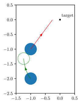
Figure 1: Motivating problem

The system is shown in Figure 1. The two blue circles represent the initial position of two balls, respectively. The pre-collision trajectory of Ball 1 is shown in green, and the post-collision trajectory of Ball 2 is shown in red. The goal is to push Ball 1 to strike Ball 2 so that Ball 2 will reach the target at the end of the simulation. We will formulate it as an optimal control problem later in Section LABEL:sec:exp. hu2022solving uses the hybrid minimum principle (HMP) to obtain an analytical solution to this class of optimal control problems. We will use this analytical solution to evaluate the performance of different methods.

3.2 Learning with Direct Velocity Impulse

An optimal control problem can be viewed as a constrained optimization problem where we design the control input at each time step to minimize an objective function. With differentiable simulation, we can compute the gradients of the objective with respect to the control inputs and use gradient-based optimization approaches to learn an optimal control sequence that minimizes the objective/loss function. Figure 2 shows the learning curves of the direct velocity impulse method implemented in Taichi and PyTorch, along with the analytically obtained optimal value. We observe that both implementations fail to converge to the analytical value even when TOI-Position is used. In Section LABEL:sec:exp, we will see that the learned control inputs do not match the analytical solution either (Figure LABEL:fig:two_balls_2_loss). This result highlights the issues present in existing differentiable simulation methods.

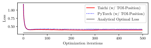
Figure 2: Learning curves of direct velocity impulse method implemented in Taichi and PyTorch.

3.3 A Hint of the Issue

To understand why the learning curve does not converge to the analytically obtained optimal solution, we initiate the learning with the analytical solution. Figure 3 shows the learning curve over the first 100 iterations. We observe that the loss jumps up in certain iterations, and the learning converges to a solution with a higher loss. This behavior is persistent across different learning rates, which indicates that the gradients computed by the differentiable simulation are incorrect.

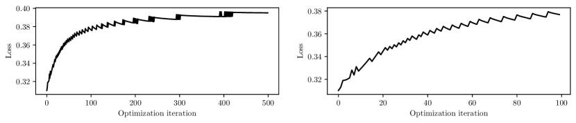
Figure 3: Motivating problem: Learning curve initialized from the analytical optimal solution.

4 Method

In this section, we first explain why the loss function increases in Figure 3 and then introduce a new technique, referred to as TOI-Velocity, to improve gradient calculation in differentiable simulation. We mainly work with a discrete-time formulation, where the simulation duration $T$ is discretized into $N$ time steps with $\Delta t=T/N$. As the examples in the paper involve two objects moving in the 2D space, we use $p_{n}=[p_{1,n},p_{2,n}]=[p_{x_{1},n},p_{y_{1},n},p_{x_{2},n},p_{y_{2},n}]$ to denote the $x$ and $y$ coordinates of the two objects at time step $n$. When we need to distinguish variables from different optimization iterations, we use the superscript $i$ to denote variables in iteration $i$.

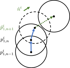
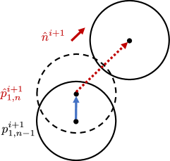
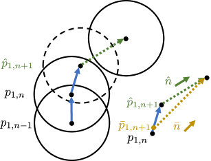
Figure 4: (a) ball positions in iteration $i$ ; (b) ball positions in iteration $i+1$ ; (c) Difference between penetration direction $\hat{n}$ and collision direction $\Bar{n}$ in an arbitrary iteration.

4.1 The Reason Behind Loss Increase

After taking a detailed look, we find that the increase of loss appears when the time step at which the collision happens changes over optimization iterations. The increase in the loss can be explained using the diagrams in Figure 4. In Figure 4, $p_{1,n-1}^{i}$ and $p_{1,n}^{i}$ show the position of the Ball 1 at time step $n-1$ and $n$ in iteration $i$, respectively. $\hat{p}_{1,n+1}^{i}$ denotes the penetrated position of Ball 1, which is an intermediate variable used to resolve the collision (explained below). The direction of the post-collision velocity of Ball 2 is determined by the penetration direction, indicated by the green arrow. Assume that after a gradient update, the position of the balls changes to the one shown in Figure 4, where the collision happens in time step $n$ instead of time step $n+1$. Now the direction of the post-collision velocity of Ball 2 is determined by the penetration direction indicated by the red arrow. As the change of penetration direction is not continuous, the change in the post-collision velocity of Ball 2 is also not continuous. Thus, the final position of Ball 2 suffers from a sudden change over these iterations, which could cause an increase in the loss since the terminal cost in the objective depends on the final position of Ball 2. This discontinuity in velocity between consecutive gradient updates is the main reason of the loss increase in Figure 3.

4.2 Time-of-impact - Velocity

To improve gradient computation in aforementioned situations where contact normal directions are not fixed, we propose to adjust post-collision velocity by continuous contact detection, and we call the technique TOI-Velocity. We present TOI-Velocity using the two-ball collision scenario shown in Figure 4, but the idea applies to collisions among multiple objects with a general class of shapes.

We assume we are using the symplectic Euler integration scheme, but the idea applies to other integration schemes as well. With symplectic Euler, we have

$$\hat{v}_{n+1} =v_{n}+u_{n}\Delta t,$$ (1)

$$\hat{p}_{n+1} =p_{n}+\hat{v}_{n+1}\Delta t,$$ (2)

where $v_{n}=[v_{1,n},v_{2,n}]=[v_{x_{1},n},v_{y_{1},n},v_{x_{2},n},v_{y_{2},n}]$ is the velocity of two balls at the $n$th time step and $u_{n}=[u_{1,n},u_{2,n}]=[u_{x_{1},n},u_{y_{1},n},u_{x_{2},n},u_{y_{2},n}]$ is the control input to the two balls at the $n$th time step. Variables with a hat ($\hat{\cdot}$) denote intermediate variables before a collision is resolved. If there is no collision detected in this time step, we would have $v_{n+1}=\hat{v}_{n+1}$ and $p_{n+1}=\hat{p}_{n+1}$. If we detect a collision as shown in Figure 4, we refer to $\hat{p}_{n+1}$ as penetration position and $\hat{v}_{n+1}$ as penetration velocity. The penetration direction is defined as $\hat{n}=(\hat{p}_{2,n+1}-\hat{p}_{1,n+1})/||\hat{p}_{2,n+1}-\hat{p}_{1,n+1}||_{2}$. Traditional simulation methods solves the post-collision velocities $v_{n+1}$ using penetration velocity $\hat{v}_{n+1}$ and penetration direction $\hat{n}$, both of which may be discontinuous across optimization iterations due to time discretization. The TOI-Position proposed by Hu2020DiffTaichi computes TOI as the time spent after the penetration appears, i.e.,

$$TOI=d/\big{(}(\hat{v}_{2,n+1}-\hat{v}_{1,n+1})\cdot\hat{n}\big{)}.$$ (3)

where $d=||\hat{p}_{2,n+1}-\hat{p}_{1,n+1}||_{2}-2r$ is the penetration depth. In other words, the collision time is estimated by $(\Delta t-TOI)$ after the balls are in position $p_{n}$. Then the post-collision position is adjusted by $p_{n+1}=p_{n}+\hat{v}_{n+1}\cdot(\Delta t-TOI)+\Tilde{v}_{n+1}\cdot TOI$, where $\Tilde{v}_{n+1}$ is the velocity after resolving collision, which depends on elasticity. However, we argue that adjusting the position only is not enough since the post-collision velocity is also incorrectly estimated. To improve that, we consider the collision position $\Bar{p}_{n+1}$ and velocity $\Bar{v}_{n+1}$