The Kolmogorov $N$-width for linear transport: Exact representation and the influence of the data

Abstract

The Kolmogorov $N$-width describes the best possible error one can achieve by elements of an $N$-dimensional linear space. Its decay has extensively been studied in Approximation Theory and for the solution of Partial Differential Equations (PDEs). Particular interest has occurred within Model Order Reduction (MOR) of parameterized PDEs e.g. by the Reduced Basis Method (RBM).

While it is known that the $N$-width decays exponentially fast (and thus admits efficient MOR) for certain problems, there are examples of the linear transport and the wave equation, where the decay rate deteriorates to $N^{-1/2}$. On the other hand, it is widely accepted that a smooth parameter dependence admits a fast decay of the $N$-width. However, a detailed analysis of the influence of properties of the data (such as regularity or slope) on the rate of the $N$-width seems to lack.

In this paper, we use techniques from Fourier Analysis to derive exact representations of the $N$-width in terms of initial and boundary conditions of the linear transport equation modeled by some function $g$ for half-wave symmetric data. For arbitrary functions $g$, we derive bounds and prove that these bounds are sharp. In particular, we prove that the $N$-width decays as ${{\color[rgb]{0,0,0}c_{r}N^{-r}}}$ for functions with Sobolev regularity $g\in H^{r{{\color[rgb]{0,0,0}-\varepsilon}}}$ for all $\varepsilon>0$ even if $g\not\in H^{r}$. Our theoretical investigations are complemented by numerical experiments which confirm the sharpness of our bounds and give additional quantitative insight.

1 Introduction

The Kolmogorov $N$-width describes the best possible error one can achieve by a linear approximation with $N\in\mathbb{N}$ degrees of freedom, i.e. by elements of the best possible $N$-dimensional linear space [1]. The arising optimal space in the sense of Kolmogorov can often not explicitly be constructed, at least not in a reasonable (computing) time. On the other hand, however, the decay rate of the $N$-width tells us if a given set can be well-approximated by a linear method, or not. This is a classical question in Approximation Theory and has been widely studied in the literature, see e.g. [2, 3, 4, 5], this list being far from complete.

Particular interest has been devoted to the case when the set to be approximated is given by solutions of certain equations, e.g. Partial Differential Equations (PDEs) with different data (one might think of the domain, coefficients, right-hand side loadings, initial- and/or boundary conditions), which might be considered as parameters [6, 7, 8]. In that direction, model order reduction of parametric PDEs (PPDE) has become a field of very intensive research, also with many very relevant real-life applications [9, 10, 11]. A prominent example is the Reduced Basis Method (RBM), where a PPDE is aimed to be reduced to an $N$-dimensional linear space in order to allow multi-query (w.r.t. different parameter values) and/or realtime (embedded systems, cloud computing) applications. The reduced $N$-dimensional system is determined in an offline training phase using sufficiently accurate detailed numerical solutions by any standard method. In this framework, the question arises, if a given PPDE can be well-reduced by means of the RBM or not. Since it has been proven in [12] that the offline reduced basis generation using a Greedy method realizes the same asymptotic rate of decay as the Kolmogorov $N$-width, one is left with the investigation of the decay for PPDEs to decide whether the RBM is suitable for a given PPDE, or not. Also in that direction, there is a significant amount of literature, e.g. [13, 14, 15, 16, 17, 18, 19, 20, 21, 22], just to name a few. Roughly speaking, it was shown there that a PPDE admits a fast decay of the $N$-width if the solution depends smoothly on the parameter, which is, e.g. known for elliptic and parabolic problems which allow for a separation of the parameters from the physical variables. As a rule of thumb: “holomorphic dependence admits exponential decay”.

However, when leaving the nice realm of such PPDEs, the situation becomes dramatically worse. It has for example been shown that the decay may drop down to $N^{-s}$, $0<s<1$, for the linear transport equation [20] and the wave equation [23]. However, the problems considered in the latter papers are quite specific examples yielding to a non-smooth dependence of the solution in terms of the parameter (the velocity in [20] and the wave speed in [23]). It was also demonstrated that the decay not only depends on the PDE, but also on the underlying physics, e.g. alloy compositions in case of solidification problems [24]. For problems of such type (transport, transport-dominated, hyperbolic), the above quoted rule of thumb remains true.

This is why we are interested in the exact dependence of the decay rate of the $N$-width in terms of the data / parameters of the problem. To our own surprise we could not find corresponding results in the literature. In [18, 21, 22], the fast decay is shown using techniques from interpolation proving that a Greedy-type selection selects the optimal nodes. The positive result in [20, Thm. 3.1] has been deduced by using the decay of the complex power series.

We consider the linear transport problem whose solution is given by the characteristics in terms of initial and boundary conditions. Hence, we can reduce ourselves to approximate the mapping $x\mapsto g(x-\mu)$, where $\mu$ is the parameter and $x\in\Omega$, which is the domain on which the PPDE is posed; $g$ is the real-valued univariate function modeling initial and boundary conditions. To this end, we use the Fourier series approximation, which allows us to incorporate the parametric shift by $\mu$ into the approximation spaces. We derive exact representations of the $N$-width for certain classes (half-wave symmetric -HWS- functions) and give estimates in terms of the regularity and the slope of the function $g$.

This paper is organized as follows. In Section 2, we collect preliminaries on the linear transport equation, the $N$-width and some facts from Fourier analysis, which we shall need in the sequel. The main tool for our analysis is a shift-isometric orthogonal decomposition (Def. 3.2) based upon the Fourier series of $g$. This notion is introduced in Section 3.2. In Section 4, we use Def. 3.2 to construct approximation spaces with which we can derive exact representations for the $N$-width for HWS functions and sharp estimates in the general case. The specific influence of the regularity of $g$ on the decay of the $N$-width is investigated in Section 5, where we prove that the $N$-width is bounded by $c_{r}N^{-r}$ for functions in the Sobolev space $H^{r{{\color[rgb]{0,0,0}-\varepsilon}}}$ for all $\varepsilon>0$ even if the function is not in $H^{r}$. In Section 6, using specifically constructed piecewise functions, we show that our bounds are sharp. Some results of our extensive numerical results are presented in Section 7. The paper finishes with some conclusions in Section 8.

2 Preliminaries

2.1 The linear transport equation

We consider the univariate linear transport equation with velocity $\mu$, which is interpreted as a parameter, i.e., we seek a function $\Phi(\cdot,\cdot;\mu):I\times\Omega\to\mathbb{R}$ such that

$$\partial_{t}\Phi(t,x;\mu)+\mu\,\partial_{x}\Phi(t,x;\mu) =0, (t,x)\in I\times\Omega,$$ (2.1a)

$$\Phi(0,x;\mu) =g(x), x\in\Omega,$$ (2.1b)

$$\Phi(t,0;\mu) =g(-\mu\,t), t\in I,$$ (2.1c)

where $I:=(0,1)$ is the time interval and $\Omega:=(0,1)$ the spatial domain. The velocity can be chosen in a compact interval $\mu\in\mathcal{P}:=[0,1]$. The initial and boundary conditions, (2.1b) and (2.1c), respectively, are given in terms of a function $g:\Omega_{\mathcal{P}}\to\mathbb{R}$, whose properties will be relevant in the sequel. Here,

$$\Omega_{\mathcal{P}}:=\{x-\mu t:x\in\Omega,\mu\in\mathcal{P},t\in I\}=(-1,1)$$

is the domain on which $g$ needs to be defined in order to obtain a well-posed problem (2.1) for every parameter. The solution of (2.1) is well-known to read $\Phi(t,x;\mu)=g(x-\mu\,t),$ $(t,x)\in I\times\Omega$. We are particularly interested in the solution at the final time $t=1$, i.e.,

$$u_{\mu}(x):=\Phi(1,x;\mu)=g(x-\mu),\qquad x\in\Omega,$$ (2.2)

and consider the low regularity case, i.e., we only assume that $g\in L_{2}(\Omega_{\mathcal{P}})$, and therefore $u_{\mu}\in L_{2}(\Omega)$, without additional smoothness.

Remark 2.1.

Often, the time $t\in I$ is also seen as a parameter. But our considerations are not restricted to the final time, since then for a given $t\in I$ and $\mu\in\mathcal{P}$, we can define the new parameter $\tilde{\mu}:=t\,\mu\in[0,1)$ and get $u_{\tilde{\mu}}=g(\cdot-\tilde{\mu})=\Phi(t,\cdot;\mu)$. $\diamond$

2.2 Linear approximation: The N-width

The specific focus of this paper is the approximation rate provided by linear subspaces. In particular, we are considering $N$-dimensional subspaces which are “optimal” to approximate $u_{\mu}$ for all parameters $\mu\in\mathcal{P}$ in an appropriate manner. Our aim is to study the dependency of the rate of approximation w.r.t. the data of the problem, namely initial and boundary conditions modeled by the function $g$. The parameter set $\mathcal{P}$ is fixed. Hence, we aim at approximating the “solution manifold”

$$\mathcal{U}_{g}:=\{u_{\mu}=g(\cdot-\mu):\,\mu\in\mathcal{P}\}\subset L_{2}(\Omega).$$ (2.3)

The maybe most classical setting is the worst case scenario w.r.t. the parameter yielding the classical Kolmogorov $N$-width [1] defined as

$$d_{N}({{\color[rgb]{0,0,0}\mathcal{U}_{g}}}) :=\kern-4.0pt\inf_{\begin{subarray}{c}V_{N}\subset L_{2}(\Omega)\\ \dim(V_{N})=N\end{subarray}}\sup_{\mu\in\mathcal{P}}\inf_{\tilde{v}_{N}\in V_{N}}\|u_{\mu}-\tilde{v}_{N}\|_{L_{2}(\Omega)}$$ (2.4)

$$=\kern-4.0pt\inf_{\begin{subarray}{c}V_{N}\subset L_{2}(\Omega)\\ \dim(V_{N})=N\end{subarray}}\operatorname{dist}(V_{N},\mathcal{U}_{g})_{L_{\infty}(\mathcal{P};L_{2}(\Omega))}.$$

The dependence on $g$ will be crucial below.

Remark 2.2.

There are several results concerning the decay of $d_{N}({{\color[rgb]{0,0,0}\mathcal{U}_{g}}})$ for the linear transport problem (2.1).

1. In [20] it was shown that $d_{N}({{\color[rgb]{0,0,0}\mathcal{U}_{g}}})$ decays as $N^{-1/2}$, i.e., very slowly for the specific choice $g=\chi_{[0,1]}$, namely for initial and boundary conditions involving a jump.

2. On the other hand, one can achieve exponential decay, i.e., $d_{N}({{\color[rgb]{0,0,0}\mathcal{U}_{g}}})\lesssim e^{-\alpha N}$ for some $\alpha>0$ if the function $g$ is analytic. This can be seen by considering a truncated power series in the complex plane [20, Thm. 3.1]. $\diamond$

Our main focus in this paper is to study the decay of the $N$-width w.r.t. properties of the function $g$, in particular we want to detail the influence of the regularity of $g$ on the decay of the $N$-width. In addition to the “worst-case in the parameter” Kolmogorov $N$-width $d_{N}({{\color[rgb]{0,0,0}\mathcal{U}_{g}}})$, which measures the error in $L_{\infty}(\mathcal{P};L_{2}(\Omega))$, we will also consider “mean-squared error in the parameter”, i.e., $L_{2}(\mathcal{P};L_{2}(\Omega))$ w.r.t. a probability measure $d\mu$ (i.e., $\int_{\mathcal{P}}d\mu=1$), which we call $L_{2}$-average $N$-width defined as

$$\delta_{N}({{\color[rgb]{0,0,0}\mathcal{U}_{g}}}) :=\inf_{\begin{subarray}{c}V_{N}\subset L_{2}(\Omega)\\ \dim(V_{N})=N\end{subarray}}\left\{\int_{\mathcal{P}}\inf_{\tilde{v}_{N}\in V_{N}}\|u_{\mu}-\tilde{v}_{N}\|_{L_{2}(\Omega)}^{2}\,d\mu\right\}^{1/2}$$ (2.5)

$$=\inf_{\begin{subarray}{c}V_{N}\subset L_{2}(\Omega)\\ \dim(V_{N})=N\end{subarray}}\operatorname{dist}(V_{N},\mathcal{U}_{g})_{L_{2}(\mathcal{P};L_{2}(\Omega))}.$$

Remark 2.3.

For later reference, we collect some equivalent expressions.

1. Let $P_{N}:L_{2}(\Omega)\to V_{N}$ denote the orthogonal projection onto $V_{N}$. Then,

   $$d_{N}({{\color[rgb]{0,0,0}\mathcal{U}_{g}}}) =\inf_{{\begin{subarray}{c}V_{N}\subset L_{2}(\Omega)\\ \operatorname{dim}(V_{N})=N\end{subarray}}}\|u_{\mu}-P_{N}u_{\mu}\|_{L_{\infty}(\mathcal{P};L_{2}(\Omega))},$$ (2.6a)

   $$\delta_{N}({{\color[rgb]{0,0,0}\mathcal{U}_{g}}}) =\inf_{{\begin{subarray}{c}V_{N}\subset L_{2}(\Omega)\\ \dim(V_{N})=N\end{subarray}}}\|u_{\mu}-P_{N}u_{\mu}\|_{L_{2}(\mathcal{P};L_{2}(\Omega))}.$$ (2.6b)

2. As $\|w\|_{L_{2}(\mathcal{P})}\leq\|w\|_{L_{\infty}(\mathcal{P})}$ for $w\in L_{\infty}(\mathcal{P})$, we get $\delta_{N}({{\color[rgb]{0,0,0}\mathcal{U}_{g}}})\leq d_{N}({{\color[rgb]{0,0,0}\mathcal{U}_{g}}})$. $\diamond$

2.3 Fourier Analysis

Our major tool for determining the decay of the $N$-widths is Fourier Analysis. Hence, we shall always assume that $g$ is periodic on the larger domain $\Omega_{\mathcal{P}}$, which is no restriction for the transport problem under consideration. We collect the main ingredients needed for the sequel of this paper. Recall that for the above model problem, we have $I=(0,1)$, $\Omega=(0,1)$, $\mathcal{P}=[0,1]$ and $\Omega_{\mathcal{P}}=(-1,1)$, but the analysis is not restricted to that case. We shall use the Fourier series of any periodic $L_{2}(\Omega_{\mathcal{P}})$-function, namely

$$g(x)=\tfrac{1}{\sqrt{2}}\hat{a}_{0}(g)+\sum_{k=1}^{\infty}\left[\hat{a}_{k}(g)\cos(k\pi x)+\hat{b}_{k}(g)\sin(k\pi x)\right],\quad x\in\Omega_{\mathcal{P}}\text{ a.e.},$$ (2.7)

where the Fourier coefficients are known as

$$\hat{a}_{0}(g)=\tfrac{1}{\sqrt{2}}\int_{\Omega_{\mathcal{P}}}\kern-5.0ptg(x)\,dx,\quad\hat{a}_{k}(g)=\langle g,\cos(k\pi\cdot)\rangle_{L_{2}(\Omega_{\mathcal{P}})},\quad\hat{b}_{k}(g)=\langle g,\sin(k\pi\cdot)\rangle_{L_{2}(\Omega_{\mathcal{P}})},$$

for $k\geq 1$. Here, we consider the space $L_{2}(\Omega_{\mathcal{P}})$ corresponding to signals of wave-length $2$. Thus, the half-wave length is $1$, which is used in the following definition, whose notion is well-known in electrical engineering (see e.g. [25]) and turns out to be crucial for the subsequent analysis.

Definition 2.4.

We call $g\in L_{2}(\Omega_{\mathcal{P}})$ even half-wave symmetric (even HWS, $g\in L_{2}^{\mathrm{evn}}$), if $g(x)=g(x+1)$ for almost all $x\in[-1,0]$, and odd half-wave symmetric (odd HWS, $g\in L_{2}^{\mathrm{odd}}$), if $g(x)=-g(x+1)$ for almost all $x\in[-1,0]$. A function is called half-wave symmetric (HWS, $g\in L_{2}^{\mathrm{hws}}$), if it is either even or odd HWS. $\diamond$

Remark 2.5.

1. The sets $\Psi^{\mathrm{evn}}:=\{\tfrac{1}{\sqrt{2}},\phi^{\mathrm{evn}}_{k},\psi^{\mathrm{evn}}_{k},k\in\mathbb{N}\}$, $\Psi^{\mathrm{odd}}:=\{\phi^{\mathrm{odd}}_{k},\psi^{\mathrm{odd}}_{k},k\in\mathbb{N}\}$ with

   $$\begin{split}\phi^{\mathrm{evn}}_{k}(x):=\cos(2k\pi x),\qquad&\psi^{\mathrm{evn}}_{k}(x):=\sin(2k\pi x),\\ \phi^{\mathrm{odd}}_{k}(x):=\cos((2k-1)\pi x),\qquad&\psi^{\mathrm{odd}}_{k}(x):=\sin((2k-1)\pi x)\end{split}$$ (2.8)

   are orthonormal bases (ONB) for $L_{2}^{\mathrm{evn}}$ and $L_{2}^{\mathrm{odd}}$, respectively.

2. We shall also need ONBs in $L_{2}(\Omega)$ and set $\tilde{\Psi}^{\mathrm{evn}}:=\{1,\tilde{\phi}^{\mathrm{evn}}_{k},\tilde{\psi}^{\mathrm{evn}}_{k},k\in\mathbb{N}\}$, $\tilde{\Psi}^{\mathrm{odd}}:=\{\tilde{\phi}^{\mathrm{odd}}_{k},\tilde{\psi}^{\mathrm{odd}}_{k},k\in\mathbb{N}\}$, where $\tilde{\xi}^{\mathrm{eo}}:=\sqrt{2}\,\xi^{\mathrm{eo}}_{|\Omega}$ for $\xi\in\{\phi,\psi\}$, $\mathrm{eo}\in\{\mathrm{evn},\mathrm{odd}\}$. We will need to keep track on this different scaling. $\diamond$

Using the Fourier expansion, it can readily be seen that any $g\in L_{2}(\Omega_{\mathcal{P}})$ can be decomposed into an even HWS and and odd HWS part, i.e., $g=g^{\mathrm{evn}}+g^{\mathrm{odd}}$, where $g^{\mathrm{evn}}\in L_{2}^{\mathrm{evn}}$ and $g^{\mathrm{odd}}\in L_{2}^{\mathrm{odd}}$, as functions on $\Omega_{\mathcal{P}}$, admit the following Fourier expansion

$$g^{\mathrm{evn}} ={{\color[rgb]{0,0,0}\tfrac{1}{\sqrt{2}}}}\hat{a}_{0}^{{{\color[rgb]{0,0,0}\mathrm{evn}}}}{{\color[rgb]{0,0,0}(g)}}+\sum_{k=1}^{\infty}\left[{{\color[rgb]{0,0,0}\hat{a}^{\mathrm{evn}}_{k}(g)\phi_{k}^{\mathrm{evn}}}}+{{\color[rgb]{0,0,0}\hat{b}^{\mathrm{evn}}_{k}(g)\psi_{k}^{\mathrm{evn}}}}\right],$$ (2.9)

$$g^{\mathrm{odd}} =\sum_{k=1}^{\infty}\left[{{\color[rgb]{0,0,0}\hat{a}^{\mathrm{odd}}_{k}(g)\phi_{k}^{\mathrm{odd}}}}+{{\color[rgb]{0,0,0}\hat{b}^{\mathrm{evn}}_{k}(g)\psi_{k}^{\mathrm{odd}}}}\right],$$ (2.10)

with the corresponding Fourier coefficients $\hat{a}_{0}^{\mathrm{evn}}(g):=\hat{a}_{0}(g)=\tfrac{1}{\sqrt{2}}\int_{\Omega}g(x)\,dx$ and

$$\hat{a}^{\mathrm{evn}}_{k}(g) :=\hat{a}_{2k}(g)=\langle g^{\mathrm{evn}},\phi_{k}^{\mathrm{evn}}\rangle_{L_{2}(\Omega_{\mathcal{P}})}=\int_{-1}^{1}g^{\mathrm{evn}}(x)\,\phi_{k}^{\mathrm{evn}}(x)\,dx$$

$$=\left\{\int_{-1}^{0}+\int_{0}^{1}\right\}g^{\mathrm{evn}}(x)\,\phi_{k}^{\mathrm{evn}}(x)\,dx=2\int_{0}^{1}g^{\mathrm{evn}}(x)\,\phi_{k}^{\mathrm{evn}}(x)\,dx$$

$$=\sqrt{2}\,\langle g^{\mathrm{evn}},\tilde{\phi}^{\mathrm{evn}}_{k}\rangle_{L_{2}(\Omega)}=2\,\langle g^{\mathrm{evn}},\cos(2k\pi\cdot)\rangle_{L_{2}(\Omega)}.$$

We collect the relations for all involved basis functions

$$\begin{split}\hat{a}^{\mathrm{evn}}_{k}(g)=\sqrt{2}\,\langle g^{\mathrm{evn}},\tilde{\phi}^{\mathrm{evn}}_{k}\rangle_{L_{2}(\Omega)},\quad&\hat{b}^{\mathrm{evn}}_{k}(g)=\sqrt{2}\,\langle g^{\mathrm{evn}},\tilde{\psi}^{\mathrm{evn}}_{k}\rangle_{L_{2}(\Omega)},\\ \hat{a}^{\mathrm{odd}}_{k}(g)=\sqrt{2}\,\langle g^{\mathrm{evn}},\tilde{\phi}^{\mathrm{odd}}_{k}\rangle_{L_{2}(\Omega)},\quad&\hat{b}^{\mathrm{odd}}_{k}(g)=\sqrt{2}\,\langle g^{\mathrm{evn}},\tilde{\psi}^{\mathrm{evn}}_{k}\rangle_{L_{2}(\Omega)}.\end{split}$$ (2.11)

We shall use this decomposition in order to determine the decay of the Kolmogorov $N$-width by splitting $g$ into its even HWS and odd HWS part and then estimating the $N$-width for both of these parts. For later reference, we collect the facts

$$L_{2}(\Omega_{\mathcal{P}})=L_{2}^{\mathrm{evn}}\oplus L_{2}^{\mathrm{odd}},\qquad L_{2}^{\mathrm{hws}}=L_{2}^{\mathrm{evn}}\cup L_{2}^{\mathrm{odd}},\qquad L_{2}^{\mathrm{hws}}\subsetneq L_{2}(\Omega_{\mathcal{P}}).$$ (2.12)

For later references, we collect some properties, which can easily be shown.

Lemma 2.6.

Let $k,\ell\in\mathbb{N}$, $x,y\in\Omega$ and $\mu\in\mathcal{P}$. Then,

$$\langle\phi^{\mathrm{odd}}_{\ell}(\cdot-\mu),\phi^{\mathrm{odd}}_{k}\rangle_{L_{2}(\Omega)} =\langle\psi^{\mathrm{odd}}_{\ell}(\cdot-\mu),\psi^{\mathrm{odd}}_{k}\rangle_{L_{2}(\Omega)}={{\color[rgb]{0,0,0}\tfrac{1}{2}}}\delta_{\ell,k}\,\phi_{k}^{\mathrm{odd}}(\mu),$$ (2.13a)

$$\langle\phi^{\mathrm{odd}}_{\ell}(\cdot-\mu),\psi^{\mathrm{odd}}_{k}\rangle_{L_{2}(\Omega)} ={{\color[rgb]{0,0,0}-}}\langle\psi^{\mathrm{odd}}_{\ell}(\cdot-\mu),\phi^{\mathrm{odd}}_{k}\rangle_{L_{2}(\Omega)}={{\color[rgb]{0,0,0}\tfrac{1}{2}}}\delta_{\ell,k}\,\psi_{k}^{\mathrm{odd}}(\mu),$$ (2.13b)

$$\phi_{\ell}^{\mathrm{odd}}(x-y) =\phi_{\ell}^{\mathrm{odd}}(x)\phi_{\ell}^{\mathrm{odd}}(y)+\psi_{\ell}^{\mathrm{odd}}(x)\psi_{\ell}^{\mathrm{odd}}(y),$$ (2.13c)

$$\phi^{\mathrm{evn}}_{k}(x-y) =\phi^{\mathrm{evn}}_{k}(x)\phi^{\mathrm{evn}}_{k}(y)+\psi^{\mathrm{evn}}_{k}(x)\psi^{\mathrm{evn}}_{k}(y),$$ (2.13d)

$$\langle\phi^{\mathrm{odd}}_{k}(x-\cdot),\phi^{\mathrm{odd}}_{\ell}(y-\cdot)\rangle_{L_{2}(\mathcal{P})} =\langle\psi^{\mathrm{odd}}_{k}(x-\cdot),\psi^{\mathrm{odd}}_{\ell}(y-\cdot)\rangle_{L_{2}(\mathcal{P})}$$

$$=\delta_{k,\ell}\,\tfrac{1}{2}\phi_{k}^{\mathrm{odd}}(x-y),$$ (2.13e)

$$\langle\phi^{\mathrm{odd}}_{k}(x-\cdot),\psi^{\mathrm{odd}}_{\ell}(y-\cdot)\rangle_{L_{2}(\mathcal{P})} ={{\color[rgb]{0,0,0}-}}\langle\psi^{\mathrm{odd}}_{k}(x-\cdot),\phi^{\mathrm{odd}}_{\ell}(y-\cdot)\rangle_{L_{2}(\mathcal{P})}$$

$$={{\color[rgb]{0,0,0}-}}\delta_{k,\ell}\,\tfrac{1}{2}\psi_{k}^{\mathrm{odd}}(x-y),$$ (2.13f)

$$\langle\phi_{\ell}^{\mathrm{evn}}(x-\cdot),\phi_{k}^{\mathrm{evn}}(y-\cdot)\rangle_{L_{2}(\mathcal{P})} =\langle\psi_{\ell}^{\mathrm{evn}}(x-\cdot),\psi_{k}^{\mathrm{evn}}(y-\cdot)\rangle_{L_{2}(\mathcal{P})}$$

$$=\tfrac{1}{2}\delta_{k,\ell}\phi^{\mathrm{evn}}_{k}(x-y),$$ (2.13g)

$$\langle\phi_{\ell}^{\mathrm{evn}}(x-\cdot),\psi_{k}^{\mathrm{evn}}(y-\cdot)\rangle_{L_{2}(\mathcal{P})} ={{\color[rgb]{0,0,0}-}}\langle\psi_{\ell}^{\mathrm{evn}}(x-\cdot),\phi_{k}^{\mathrm{evn}}(y-\cdot)\rangle_{L_{2}(\mathcal{P})}$$

$$={{\color[rgb]{0,0,0}-}}\tfrac{1}{2}\delta_{k,\ell}\psi^{\mathrm{evn}}_{k}(x-y),$$ (2.13h)

$$\hat{a}_{k}^{\mathrm{evn}}(g)=\langle g,\phi_{k}^{\mathrm{evn}}\rangle_{L_{2}(\Omega_{\mathcal{P}})}, \quad\hat{b}_{k}^{\mathrm{evn}}(g)=\langle g,\psi_{k}^{\mathrm{evn}}\rangle_{L_{2}(\Omega_{\mathcal{P}})},$$ (2.13i)

$$\hat{a}_{k}^{\mathrm{odd}}(g)=\langle g,\phi_{k}^{\mathrm{odd}}\rangle_{L_{2}(\Omega_{\mathcal{P}})}, \quad\hat{b}_{k}^{\mathrm{odd}}(g)=\langle g,\psi_{k}^{\mathrm{odd}}\rangle_{L_{2}(\Omega_{\mathcal{P}})}.$$ (2.13j)

2.4 Sobolev spaces of broken order

Our main goal is to relate the decay of the Kolmogorov $N$-width to the regularity of the solution w.r.t. the parameter. To this end, we consider the Sobolev space of order $r>0$ by

$$H^{r}(\Omega_{\mathcal{P}}) :=\left\{g\text{ as in \eqref{eq:Fourier}}:\sum_{k=1}^{\infty}(1+k^{2})^{r}\left(\hat{a}_{k}^{2}+\hat{b}_{k}^{2}\right)<\infty\right\}.$$ (2.14)

As we need to distinguish even and odd half-wave symmetric functions, we set

$$H^{r,\mathrm{odd}}(\Omega) :=\left\{\sum_{k=1}^{\infty}\big{[}\hat{a}^{\mathrm{odd}}_{k}\tilde{\phi}^{\mathrm{odd}}_{k}+\hat{b}^{\mathrm{odd}}_{k}\tilde{\psi}^{\mathrm{odd}}_{k}\big{]}\!\!:\,\sum_{k=1}^{\infty}(1+k^{2})^{r}\left((\hat{a}^{\mathrm{odd}}_{k})^{2}+(\hat{b}^{\mathrm{odd}}_{k})^{2}\right)<\infty\right\}.$$

and similarly for the even case (adding the constant basis function, of course). This can also be rephrased as follows for $\mathrm{eo}\in\{\mathrm{evn},\mathrm{odd}\}$

$$f\in H^{r,\mathrm{eo}}(\Omega) \iff\hat{\bm{f}}^{\mathrm{eo}}\in\ell_{2,r},$$ (2.15)

where $\ell_{2,r}:=\{\bm{c}\in\ell_{2}(\mathbb{N}):\,\|\bm{c}\|_{2,r}^{2}:=\sum_{k=1}^{\infty}(1+k^{2})^{r}c_{k}^{2}<\infty\}$ is the weighted sequence space and $\hat{\bm{f}}^{\mathrm{eo}}=(\hat{f}^{\mathrm{eo}}_{k})_{k\in\mathbb{N}}$, $(\hat{f}^{\mathrm{eo}}_{k})^{2}:=(\hat{a}^{\mathrm{eo}}_{k})^{2}+(\hat{b}^{\mathrm{eo}}_{k})^{2}$ is the sequence of Fourier coefficients.

3 Orthogonal space decomposition

Since the orthogonal projection is the best approximation, we are considering orthogonal decompositions of the spaces that are relevant for the transport problem. We find that the orthogonal space decompositions need to be tailored to a given function g in order to bound or represent $d_{N}({{\color[rgb]{0,0,0}\mathcal{U}_{g}}})$ and $\delta_{N}({{\color[rgb]{0,0,0}\mathcal{U}_{g}}})$ for that function $g$.

3.1 Eigenspaces and optimality

Spaces spanned by eigenfunctions are expectedly relevant for analyzing the $L_{2}$-average $N$-width $\delta_{N}({{\color[rgb]{0,0,0}\mathcal{U}_{g}}})$. In fact, it is not surprising that this leads us to spaces spanned by eigenfunctions. In fact, the appropriate orthogonal space decomposition is built by eigenspaces of the operator induced by the bilinear form

$$k^{g}:L_{2}(\Omega)\times L_{2}(\Omega)\to\mathbb{R},\qquad k^{g}(v,w):=\int_{\mathcal{P}}\langle u_{\mu},v\rangle_{L_{2}(\Omega)}\,\langle u_{\mu},w\rangle_{L_{2}(\Omega)}\,d\mu$$

with the “snapshots” $u_{\mu}=g(\cdot-\mu)$ induced by the function $g$ are defined by (2.2). We need to keep track on the dependence on $g$. Obviously, $k^{g}$ is a symmetric and positive semi-definite bilinear form. We define the induced operator by

$$\mathcal{K}^{g}:L_{2}(\Omega)\to L_{2}(\Omega),\qquad\langle\mathcal{K}^{g}\varphi,\psi\rangle_{L_{2}(\Omega)}:=k^{g}(\varphi,\psi),\,\psi\in L_{2}(\Omega),$$

which is obviously a positive semi-definite operator.

Remark 3.1.

We note the following representation of $k^{g}$ (and hence $\mathcal{K}^{g}$):

$$k^{g}(v,w) =\int_{\Omega}\int_{\Omega}v(x)\kappa^{g}(x,y)w(y)\,dy\,dx,$$

where $\kappa^{g}(x,y):=\langle u_{\mu}(x),u_{\mu}(y)\rangle_{L_{2}(\mathcal{P})}=\int_{\mathcal{P}}g(x-\mu)\,g(y-\mu)\,d\mu$, i.e., $k^{g}$ is an integral operator with kernel $\kappa^{g}$. $\diamond$

The operator $\mathcal{K}^{g}$ admits an $L_{2}(\Omega)$-ON basis $\{v^{g}_{k}\}_{k\in\mathbb{N}}$ of eigenfunctions according to non-negative ordered eigenvalues $\lambda^{g}_{1}\geq\lambda^{g}_{2}\geq\cdots\geq 0$. Then, we define

$$V^{g}_{N}:=\operatorname{span}\{v^{g}_{1},...,v^{g}_{N}\}$$

along with the orthogonal projector $P_{N}^{g}:L_{2}(\Omega)\to V^{g}_{N}$ defined as $P_{N}^{g}v:=\sum_{k=1}^{N}\langle v,v^{g}_{k}\rangle_{L_{2}(\Omega)}\,v^{g}_{k}$. The spaces $V_{N}^{g}$ will be constructed via a family of subspaces $\mathcal{W}^{g}:=\{W_{k}^{g}\}_{k\in\mathbb{N}}\subset L_{2}(\Omega)$ along with the associated orthogonal projectors $\mathcal{Q}^{g}:=\{Q_{k}^{g}\}_{k\in\mathbb{N}}$, $Q_{k}^{g}:L_{2}(\Omega)\to W_{k}^{g}$ forming an orthogonal decomposition, i.e., $L_{2}(\Omega)=\overline{\bigoplus_{k=1}^{\infty}W_{k}^{g}}$ and $W_{k}^{g}\perp W_{j}^{g}$ for $j\neq k$. By orthonormality, we have

$$\operatorname{dist}(V^{g}_{N},\mathcal{U}(\mathcal{P}))_{L_{2}(\mathcal{P};L_{2}(\Omega))}^{2} =\int_{\mathcal{P}}\|u_{\mu}-P^{g}_{N}u_{\mu}\|_{L_{2}(\Omega)}^{2}\,d\mu=\sum_{k=N+1}^{\infty}\int_{\mathcal{P}}\langle u_{\mu},v^{g}_{k}\rangle_{L_{2}(\Omega)}^{2}\,d\mu$$

$$=\sum_{k=N+1}^{\infty}\int_{\mathcal{P}}k^{g}(v^{g}_{k},v^{g}_{k})\,d\mu=\sum_{k=N+1}^{\infty}\lambda_{k}^{g}=\delta_{N}({{\color[rgb]{0,0,0}\mathcal{U}_{g}}})^{2},$$ (3.1)

where the last step follows from the fact that the eigenvalues are ordered. In this sense, eigenspaces are optimal in $L_{2}$, which is oft course quite well-known from the Singular Value Decomposition (SVD) or the Proper Orthogonal Decomposition (POD) in MOR. However, for analyzing the $N$-width, we need to identify the eigenfunctions in such a way that the eigenvalues are ordered as above.

3.2 Shift-isometry

In order to link $\delta_{N}({{\color[rgb]{0,0,0}\mathcal{U}_{g}}})$ to the $L_{\infty}$-based $N$-width $d_{N}({{\color[rgb]{0,0,0}\mathcal{U}_{g}}})$, we need an additional property of an orthogonal decomposition to be introduced next.

Definition 3.2.

Let $g\in L_{2}(\Omega_{\mathcal{P}})$. An orthogonal space decomposition of $L_{2}(\Omega)$ induced by a family of subspaces $\mathcal{W}^{g}:=\{W_{k}^{g}\}_{k\in\mathbb{N}}$ with the associated orthogonal projectors $\mathcal{Q}^{g}:=\{Q_{k}^{g}\}_{k\in\mathbb{N}}$, $Q_{k}^{g}:L_{2}(\Omega)\to W_{k}^{g}$ is called shift-isometric orthogonal decomposition (w.r.t. $g$) of $L_{2}(\Omega)$ if

$$\|Q_{k}^{g}g(\cdot-\mu)\|_{L_{2}(\Omega)}=\|Q_{k}^{g}g\|_{L_{2}(\Omega)}\quad\text{for all }\mu\in\mathcal{P}.$$ (3.2)

i.e., if the orthogonal projectors are shift-isometric. $\diamond$

Remark 3.3.

Note, that $g$ needs to be defined on the larger space $\Omega_{\mathcal{P}}$ in order to apply $g(\cdot-\mu)$. However, the solution of the transport problem (2.1) is defined on the domain $\Omega$. Whenever we take a norm $\|\cdot\|_{L_{2}(\Omega)}$ or apply $Q_{k}^{g}$, we consider implicitly the restrictions $g_{|\Omega}$ or $g(\cdot-\mu)_{|\Omega}$ respectively. $\diamond$

Now, we start by assuming that such a $\mathcal{W}^{g}$ exists and show that (3.2) is a key property. If $\mathcal{W}^{g}$ is a (shift-isometric) orthogonal decomposition of $L_{2}(\Omega)$, each $u_{\mu}\in\mathcal{U}_{g}\subset L_{2}(\Omega)$ has a unique decomposition $u_{\mu}=\sum_{k=1}^{\infty}Q_{k}^{g}u_{\mu}$. We define

$$V_{N}^{g}:=\bigoplus_{k=1}^{M(N)}W_{k}^{g},\quad\text{where }N=\dim(V_{N}^{g})=\sum_{k=1}^{M(N)}\dim(W_{k}^{g})$$ (3.3)

as a candidate for the best approximation space in the sense of Kolmogorov. Later, the spaces $W^{g}_{k}$ will be spanned by two eigenfunctions corresponding to the same eigenvalue. Clearly, the approximation $\tilde{v}_{N}:=\sum_{k=1}^{M(N)}Q_{k}^{g}u_{\mu}$ converges to $u_{\mu}$ as $N\to\infty$, which implies that both $d_{N}({{\color[rgb]{0,0,0}\mathcal{U}_{g}}})$ and $\delta_{N}({{\color[rgb]{0,0,0}\mathcal{U}_{g}}})$ converge towards zero. Moreover, the orthogonality easily allows us to control the error.

Proposition 3.4.

Let $g\in L_{2}(\Omega_{\mathcal{P}})$, let $\mathcal{W}^{g}$ be a corresponding shift-isometric orthogonal decomposition of $L_{2}(\Omega)$ and let $V_{N}^{g}$ be defined as in (3.3). Then,

$$\operatorname{dist}(V_{N}^{g},\mathcal{U}_{g})_{L_{\infty}(\mathcal{P};L_{2}(\Omega))}^{2} \kern-2.0pt=\operatorname{dist}(V_{N}^{g},\mathcal{U}_{g})_{L_{2}(\mathcal{P};L_{2}(\Omega))}^{2}\kern-2.0pt=\kern-10.0pt\sum_{k=M(N)+1}^{\infty}\kern-10.0pt\|Q_{k}^{g}g\|_{L_{2}(\Omega)}^{2}.$$ (3.4)

Proof.

The second equality is given by (3.1). Concering $L_{\infty}(\mathcal{P})$, we get by shift-isometry (Def. 3.2) $\|Q_{k}^{g}u_{\mu}\|_{L_{2}(\Omega)}=\|Q_{k}^{g}g(\cdot-\mu)\|_{L_{2}(\Omega)}=\|Q_{k}^{g}g\|_{L_{2}(\Omega)}$, so that

$$\operatorname{dist}(V_{N}^{g},\mathcal{U}_{g})_{L_{\infty}(\mathcal{P};L_{2}(\Omega))}^{2} =\sup_{\mu\in\mathcal{P}}\|u_{\mu}-P_{N}^{g}u_{\mu}\|_{L_{2}(\Omega)}^{2}$$

$$\kern-100.0pt=\sup_{\mu\in\mathcal{P}}\sum_{k=M(N)+1}^{\infty}\|Q_{k}^{g}g\|_{L_{2}(\Omega)}^{2}=\sum_{k=M(N)+1}^{\infty}\kern-10.0pt\|Q_{k}^{g}g\|_{L_{2}(\Omega)}^{2}$$

$$\kern-100.0pt=\int_{\mathcal{P}}\sum_{k=M(N)+1}^{\infty}\kern-10.0pt\|Q_{k}^{g}g\|_{L_{2}(\Omega)}^{2}d\mu=\operatorname{dist}(V_{N}^{g},\mathcal{U}_{g})_{L_{2}(\mathcal{P};L_{2}(\Omega))}^{2},$$

since $d\mu$ is a probability measure, which completes the proof. ∎

Remark 3.5.

From Proposition 3.4 and the previous discussion we see that $\delta_{N}(\mathcal{U}_{g})=d_{N}(\mathcal{U}_{g})$ and since the optimal spaces $V_{N}^{g}$ in the sense of Kolmogorov are formed by eigenfunctions corresponding to the largest eigenvalues of the operator $\mathcal{K}^{g}$, we conclude that $\|Q_{k}^{g}g\|_{L_{2}(\Omega)}^{2}=m_{k}\,\lambda^{g}_{k}$, where $m_{k}$ is the algebraic multiplicity of $\lambda^{g}_{k}$. $\diamond$

Before continuing, we stress that for shift-isometric decompositions both versions of the $N$-width coincide and that the right-hand side of (3.4) is independent of the parameter $\mu$, which allows us to bound the $N$-width for all parameters. As the simple proof above shows, the shift-isometry (3.2) is the key property.

4 N-widths for half-wave symmetric functions

We are now going to construct shift-isometric orthogonal decompositions for half-wave symmetric functions $g\in{{\color[rgb]{0,0,0}L_{2}^{\mathrm{hws}}}}$ in terms of trigonometric functions. This will allow us to define spaces $W_{k}^{\mathrm{hws}}\subset L_{2}(\Omega)$ which have an additional property, namely they are shift-invariant, i.e., if $w\in W_{k}^{\mathrm{hws}}$, then ${{\color[rgb]{0,0,0}w(\cdot-\mu+\chi_{[0,\mu]}(\cdot))}}\in W_{k}^{\mathrm{hws}}$ for all $\mu\in\mathcal{P}$. We will need to consider even and odd HWS functions separately.

We restrict ourselves to $\mathcal{P}=[0,1]$ and choose $d\mu$ as the Lebesgue measure, i.e., $L_{2}(\mathcal{P})=L_{2}(\Omega)$. Before we continue, we would like to stress one technical challenge. We have to deal with bases in $L_{2}(\Omega)$ and $L_{2}(\Omega_{\mathcal{P}})$. We will use functions defined on all $\mathbb{R}$ and consider their restriction to $\Omega$ and $\Omega_{\mathcal{P}}$. We shall always try to clearly indicate which domain is meant.

4.1 Even half-wave symmetric functions

Lemma 4.1.

For any $k\in\mathbb{N}$, the set $\{\tilde{\phi}_{k}^{\mathrm{evn}},\tilde{\psi}_{k}^{\mathrm{evn}}\}\subset{L_{2}(\Omega)}$ is an orthonormal basis for $W_{k}^{\mathrm{evn}}:=\operatorname{span}\{\tilde{\phi}_{k}^{\mathrm{evn}},\tilde{\psi}_{k}^{\mathrm{evn}}\}$ with $\dim(W_{k}^{\mathrm{evn}})=2$ and these spaces are shift-invariant.

Proof.

The statements concerning orthonormality and dimension are straightforward. Let $\mu\in\mathcal{P}$ and $x\in\Omega$, then

$${{\color[rgb]{0,0,0}\tilde{\phi}^{\mathrm{evn}}_{k}(x-\mu)}} ={{\color[rgb]{0,0,0}\sqrt{2}}}\,\cos\big{(}2k\pi\mu\big{)}\sin\big{(}2k\pi x\big{)}-{{\color[rgb]{0,0,0}\sqrt{2}}}\,\sin\big{(}2k\pi\mu\big{)}\cos\big{(}2k\pi x\big{)}$$

$$=:a_{k,1}(\mu)\,{{\color[rgb]{0,0,0}\tilde{\phi}^{\mathrm{evn}}_{k}}}(x)+a_{k,2}(\mu)\ {{\color[rgb]{0,0,0}\tilde{\psi}^{\mathrm{evn}}_{k}}}(x)$$

and therefore ${{\color[rgb]{0,0,0}\tilde{\phi}^{\mathrm{evn}}_{k}}}(\cdot-\mu)\in W_{k}^{\mathrm{evn}}$. The same applies for ${{\color[rgb]{0,0,0}\tilde{\psi}^{\mathrm{evn}}_{k}}}$. ∎

The simple proof shows that $W_{k}^{\mathrm{evn}}=\{\alpha\,\sin(2k\pi\cdot+\beta):\,\alpha,\beta\in\mathbb{R}\}$. For $k=0$, we set $W_{0}^{\mathrm{\mathrm{evn}}}:=\operatorname{span}\{{{\color[rgb]{0,0,0}1}}\},\dim(W_{0}^{\mathrm{\mathrm{evn}}})=1$, i.e., the constant functions.

Remark 4.2.

The above definition is similar to Kolmogorov’s paper in 1936 [1], where the best basis functions for all periodic $H^{r}(0,1)$-functions with $\|f^{(r)}\|_{L_{2}(0,1)}\leq 1$ is shown to be $\{1$, $\sqrt{2}\sin\left(2\pi kx\right)$, $\sqrt{2}\cos\left(2\pi kx\right)$, $k=1,2,...,\tfrac{N-1}{2}\}$. For such classes of functions, Kolmogorov quantified a constant, which was later called Kolmogorov $N$-width in honor of his contributions and proved $d_{N}=(\pi N)^{-r}$. $\diamond$

Lemma 4.3.

Let $g\in L_{2}^{\mathrm{evn}}$. Then, $\tilde{\phi}_{k}^{\mathrm{evn}}$ and $\tilde{\psi}_{k}^{\mathrm{evn}}$, $k\in\mathbb{N}$, are $L_{2}(\Omega)$-normalized eigenfunctions of $\mathcal{K}^{g}$ to the eigenvalues (recall (2.11))

$$\lambda_{2k}^{\mathrm{evn}}(g)=\lambda_{2k-1}^{\mathrm{evn}}(g)=\tfrac{1}{4}(\hat{a}_{k}^{\mathrm{evn}}(g)^{2}+\hat{b}_{k}^{\mathrm{evn}}(g)^{2}).$$ (4.1)

Proof.

The set $\{{{\color[rgb]{0,0,0}\tfrac{1}{\sqrt{2}}}},\phi^{\mathrm{evn}}_{\ell},\psi_{\ell}^{\mathrm{evn}},\ell\in\mathbb{N}\}$ is an ONB for $L_{2}^{\mathrm{evn}}$. Hence, any $g\in L_{2}^{\mathrm{evn}}$ has an expansion of the form (2.9). Then,

$$\kappa^{g}(x,y) =\int_{\mathcal{P}}g(x-\mu)\,g(y-\mu)\,d\mu$$

$$\hskip-25.0pt=\int_{\mathcal{P}}\Bigg{[}\tfrac{1}{\sqrt{2}}\hat{a}_{0}^{\mathrm{evn}}(g)+\sum_{\ell=1}^{\infty}\Big{(}\hat{a}_{\ell}^{\mathrm{evn}}(g)\,\phi_{\ell}^{\mathrm{evn}}(x-\mu)+\hat{b}_{\ell}^{\mathrm{evn}}(g)\,\psi_{\ell}^{\mathrm{evn}}(x-\mu)\Big{)}\Bigg{]}$$

$$\hskip 5.0pt\times\Bigg{[}\tfrac{1}{\sqrt{2}}\hat{a}_{0}^{\mathrm{evn}}(g)+\sum_{k=1}^{\infty}\Big{(}\hat{a}_{k}^{\mathrm{evn}}(g)\,\phi_{k}^{\mathrm{evn}}(x-\mu)+\hat{b}_{k}^{\mathrm{evn}}(g)\,\psi_{k}^{\mathrm{evn}}(y-\mu)\Big{)}\Bigg{]}\,d\mu$$

$$\hskip-25.0pt=\hat{a}_{0}^{\mathrm{evn}}(g)^{2}+\tfrac{1}{\sqrt{2}}\hat{a}_{0}^{\mathrm{evn}}(g)\sum_{\ell=1}^{\infty}\Big{(}\hat{a}_{\ell}^{\mathrm{evn}}(g)\,\underbrace{\int_{\mathcal{P}}\phi_{\ell}^{\mathrm{evn}}(x-\mu)\,d\mu}_{=0}+\hat{b}_{\ell}^{\mathrm{evn}}(g)\,\underbrace{\int_{\mathcal{P}}\psi_{\ell}^{\mathrm{evn}}(x-\mu)\,d\mu}_{=0}\Big{)}$$

$$\hskip 5.0pt+\tfrac{1}{\sqrt{2}}\hat{a}_{0}^{\mathrm{evn}}(g)\sum_{k=1}^{\infty}\Big{(}\hat{a}_{k}^{\mathrm{evn}}(g)\,\underbrace{\int_{\mathcal{P}}\phi_{\ell}^{\mathrm{evn}}(y-\mu)\,d\mu}_{=0}+\hat{b}_{k}^{\mathrm{evn}}(g)\,\underbrace{\int_{\mathcal{P}}\psi_{k}^{\mathrm{evn}}(y-\mu)\,d\mu}_{=0}\Big{)}$$

$$\hskip 5.0pt+\sum_{k,\ell=1}^{\infty}\Big{\{}\hat{a}_{\ell}^{\mathrm{evn}}(g)\,\hat{a}_{k}^{\mathrm{evn}}(g)\,\underbrace{\langle\phi_{\ell}^{\mathrm{evn}}(x-\cdot),\phi_{k}^{\mathrm{evn}}(y-\cdot)\rangle_{L_{2}(\mathcal{P})}}_{=\tfrac{1}{2}\delta_{k,\ell}\phi^{\mathrm{evn}}_{k}(x-y),\text{ by }\eqref{eq:SimpleProperties:9}}$$

$$\hskip 50.0pt+\hat{a}_{\ell}^{\mathrm{evn}}(g)\,\hat{b}_{k}^{\mathrm{evn}}(g)\,\langle\phi_{\ell}^{\mathrm{evn}}(x-\cdot),\psi_{k}^{\mathrm{evn}}(y-\cdot)\rangle_{L_{2}(\mathcal{P})}$$

$$\hskip 50.0pt+\hat{b}_{\ell}^{\mathrm{evn}}(g)\,\hat{a}_{k}^{\mathrm{evn}}(g)\,\langle\psi_{\ell}^{\mathrm{evn}}(x-\cdot),\phi_{k}^{\mathrm{evn}}(y-\cdot)\rangle_{L_{2}(\mathcal{P})}$$

$$\hskip 50.0pt+\hat{b}_{\ell}^{\mathrm{evn}}(g)\,\hat{b}_{k}^{\mathrm{evn}}(g)\,\underbrace{\langle\psi_{\ell}^{\mathrm{evn}}(x-\cdot),\psi_{k}^{\mathrm{evn}}(y-\cdot)\rangle_{L_{2}(\mathcal{P})}}_{=\tfrac{1}{2}\delta_{k,\ell}\phi^{\mathrm{evn}}_{k}(x-y),\text{ by }\eqref{eq:SimpleProperties:9}}\Big{\}}.$$

$$\hskip-25.0pt=\hat{a}_{0}^{\mathrm{evn}}(g)^{2}+\tfrac{1}{2}\sum_{\ell=1}^{\infty}\big{(}\hat{a}_{\ell}^{\mathrm{evn}}(g)^{2}+\hat{b}_{\ell}^{\mathrm{evn}}(g)^{2}\big{)}\phi^{\mathrm{evn}}_{k}(x-y),$$

since the sum of the two middle terms vanishes by (2.13h). Thus, for any $w\in L_{2}(\Omega)$,

$$k^{g}(\tilde{\phi}_{k}^{\mathrm{evn}},w) =\int_{\Omega}\int_{\Omega}\tilde{\phi}_{k}^{\mathrm{evn}}(x)\,k^{g}(x,y)\,w(y)\,dy\,dx$$

$$\hskip-35.0pt=\int_{\Omega}\int_{\Omega}\tilde{\phi}_{k}^{\mathrm{evn}}(x)\,\bigg{[}\hat{a}_{0}^{\mathrm{evn}}(g)^{2}+\tfrac{1}{2}\sum_{\ell=1}^{\infty}\big{(}\hat{a}_{\ell}^{\mathrm{evn}}(g)^{2}+\hat{b}_{\ell}^{\mathrm{evn}}(g)^{2}\big{)}\phi^{\mathrm{evn}}_{\ell}(x-y)\bigg{]}w(y)\,dy\,dx$$

$$\hskip-35.0pt=\hat{a}_{0}^{\mathrm{evn}}(g)^{2}\int_{\Omega}w(y)\,dy\,\underbrace{\int_{\Omega}\tilde{\phi}_{k}^{\mathrm{evn}}(x)\,dx}_{=0}$$

$$\hskip 15.0pt+\tfrac{1}{2}\sum_{\ell=1}^{\infty}\big{(}\hat{a}_{\ell}^{\mathrm{evn}}(g)^{2}+\hat{b}_{\ell}^{\mathrm{evn}}(g)^{2}\big{)}\Big{\{}\underbrace{\langle\tilde{\phi}_{k}^{\mathrm{evn}},\phi_{\ell}^{\mathrm{evn}}\rangle_{L_{2}(\Omega)}}_{=\tfrac{\sqrt{2}}{2}\,\delta_{\ell,k}\text{ by }\eqref{eq:SimpleProperties:9}}\,\langle\phi_{\ell}^{\mathrm{evn}},w\rangle_{L_{2}(\Omega)}$$

$$\hskip 130.0pt+\underbrace{\langle\tilde{\phi}_{k}^{\mathrm{evn}},\psi_{\ell}^{\mathrm{evn}}\rangle_{L_{2}(\Omega)}}_{=0\text{ by }\eqref{eq:SimpleProperties:10}}\,\langle\psi_{\ell}^{\mathrm{evn}},w\rangle_{L_{2}(\Omega)}\Big{\}}$$

$$\hskip-35.0pt=\tfrac{\sqrt{2}}{4}\big{(}\hat{a}_{k}^{\mathrm{evn}}(g)^{2}+\hat{b}_{k}^{\mathrm{evn}}(g)^{2}\big{)}\,\langle\phi_{k}^{\mathrm{evn}},w\rangle_{L_{2}(\Omega)}=\lambda_{2k}^{\mathrm{evn}}(g)\,\langle\tilde{\phi}_{k}^{\mathrm{evn}},w\rangle_{L_{2}(\Omega)},$$

which proves the claim for $\tilde{\phi}_{k}^{\mathrm{evn}}$. A similar derivation applies to $\tilde{\psi}_{k}^{\mathrm{evn}}$ from which we deduce that $\lambda_{2k}^{\mathrm{evn}}(g)=\lambda_{2k-1}^{\mathrm{evn}}(g)$. ∎

4.2 Odd half-wave symmetric functions

In a quite analogous manner, we get a similar result for the odd half-wave symmetric case. We skip the proofs.

Lemma 4.4.

For any $k\in\mathbb{N}$, the set $\{\tilde{\phi}_{k}^{\mathrm{odd}},\tilde{\psi}_{k}^{\mathrm{odd}}\}\subset{L_{2}(\Omega)}$ is an orthonormal basis of the shift-invariant spaces $W_{k}^{\mathrm{odd}}:=\operatorname{span}\{\tilde{\phi}_{k}^{\mathrm{odd}},\tilde{\psi}_{k}^{\mathrm{odd}}\}$ with $\dim(W_{k}^{\mathrm{odd}})=2$. ∎

Lemma 4.5.

Let $g\in L_{2}^{\mathrm{odd}}$. Then, $\tilde{\phi}_{k}^{\mathrm{odd}}$ and $\tilde{\psi}_{k}^{\mathrm{odd}}$, $k\in\mathbb{N}$, are $L_{2}(\Omega)$-normalized eigenfunctions of $\mathcal{K}^{g}$ to the eigenvalues (recall (2.11))

$$\lambda_{2k}^{\mathrm{odd}}(g)=\lambda_{2k-1}^{\mathrm{odd}}(g)=\tfrac{1}{4}(\hat{a}_{k}^{\mathrm{odd}}(g)^{2}+\hat{b}_{k}^{\mathrm{odd}}(g)^{2}).$$ (4.2)

4.3 Shift-isometry

We shall now prove that the above construction yields shift-isometric orthogonal decompositions. It turns out that shift-isometry (Def. 3.2 (ii)) and half-wave symmetry allow us to use the same orthogonal decomposition of $L_{2}(\Omega)$ for all $L_{2}^{\mathrm{evn}}$- and $L_{2}^{\mathrm{odd}}$-functions, respectively. We do not need a specific decomposition $\mathcal{W}^{g}$ for each individual function $g\in L_{2}^{\mathrm{hws}}$.

Lemma 4.6.

1. The family $\mathcal{W}^{\mathrm{evn}}:=\{W_{k}^{\mathrm{evn}}\}_{k\in\mathbb{N}_{0}}$ is a shift-isometric orthogonal decomposition of $L_{2}(\Omega)$ w.r.t. all $g\in L_{2}^{\mathrm{evn}}$.

2. The family $\mathcal{W}^{\mathrm{odd}}:=\{W_{k}^{\mathrm{odd}}\}_{k\in\mathbb{N}}$ is a shift-isometric orthogonal decomposition of $L_{2}(\Omega)$ w.r.t. all $g\in L_{2}^{\mathrm{odd}}$.

Proof.

We restrict ourselves to the odd case since the even case is analogous. We start by considering some $g^{\mathrm{odd}}\in L_{2}^{\mathrm{odd}}$, which has the Fourier expansion (2.10). Recalling (2.11), we expand $g^{\mathrm{odd}}(\cdot-\mu)$ in $L_{2}(\Omega)$ as follows

$$g^{\mathrm{odd}}(\cdot-\mu) ={{\color[rgb]{0,0,0}\sum_{\ell=1}^{\infty}\Big{(}\langle g,\tilde{\phi}_{k}^{\mathrm{evn}}\rangle_{L_{2}(\Omega)}\,\tilde{\phi}_{k}^{\mathrm{evn}}(\cdot-\mu)+\langle g,\tilde{\psi}_{k}^{\mathrm{evn}}\rangle_{L_{2}(\Omega)}\,\tilde{\psi}_{k}^{\mathrm{evn}}(\cdot-\mu)\Big{)}}}$$

$$=\sum_{\ell=1}^{\infty}\Big{(}{{\color[rgb]{0,0,0}\hat{a}_{\ell}^{\mathrm{odd}}}}\,{{\color[rgb]{0,0,0}\tilde{\phi}^{\mathrm{odd}}_{\ell}}}(\cdot-\mu)+{{\color[rgb]{0,0,0}\hat{b}_{\ell}^{\mathrm{odd}}}}\,{{\color[rgb]{0,0,0}\tilde{\psi}^{\mathrm{odd}}_{\ell}}}(\cdot-\mu)\Big{)}.$$ (4.3)

From this we can compute the orthogonal projection, which is defined as

$$\kern 0.0ptQ_{k}^{\mathrm{odd}}g^{\mathrm{odd}}(\cdot-\mu)=\langle g^{\mathrm{odd}}(\cdot-\mu),{{\color[rgb]{0,0,0}\tilde{\phi}^{\mathrm{odd}}_{k}}}\rangle_{L_{2}(\Omega)}{{\color[rgb]{0,0,0}\tilde{\phi}^{\mathrm{odd}}_{k}}}+\langle g^{\mathrm{odd}}(\cdot-\mu),{{\color[rgb]{0,0,0}\tilde{\psi}^{\mathrm{odd}}_{k}}}\rangle_{L_{2}(\Omega)}{{\color[rgb]{0,0,0}\tilde{\psi}^{\mathrm{odd}}_{k}}}.$$ (4.4)

Next, we insert (4.6) into (4.4) and use (2.13a), (2.13b), so that

$$Q_{k}^{\mathrm{odd}}g^{\mathrm{odd}}(\cdot-\mu) =\langle{{\color[rgb]{0,0,0}\hat{a}_{k}^{\mathrm{odd}}}}{{\color[rgb]{0,0,0}\tilde{\phi}^{\mathrm{odd}}_{k}}}(\cdot-\mu)+{{\color[rgb]{0,0,0}\hat{b}_{k}^{\mathrm{odd}}}}{{\color[rgb]{0,0,0}\tilde{\psi}^{\mathrm{odd}}_{k}}}(\cdot-\mu),{{\color[rgb]{0,0,0}\tilde{\phi}^{\mathrm{odd}}_{k}}}\rangle_{L_{2}(\Omega)}{{\color[rgb]{0,0,0}\tilde{\phi}^{\mathrm{odd}}_{k}}}$$

$$\hskip 15.0pt+\langle{{\color[rgb]{0,0,0}\hat{a}_{k}^{\mathrm{odd}}}}{{\color[rgb]{0,0,0}\tilde{\phi}^{\mathrm{odd}}_{k}}}(\cdot-\mu)+{{\color[rgb]{0,0,0}\hat{b}_{k}^{\mathrm{odd}}}}{{\color[rgb]{0,0,0}\tilde{\psi}^{\mathrm{odd}}_{k}}}(\cdot-\mu),{{\color[rgb]{0,0,0}\tilde{\psi}^{\mathrm{odd}}_{k}}}\rangle_{L_{2}(\Omega)}{{\color[rgb]{0,0,0}\tilde{\psi}^{\mathrm{odd}}_{k}}}$$

$$\kern-50.0pt=[{{\color[rgb]{0,0,0}\hat{a}_{k}^{\mathrm{odd}}\phi_{k}^{\mathrm{odd}}(\mu)}}+{{\color[rgb]{0,0,0}\hat{b}_{k}^{\mathrm{odd}}\psi_{k}^{\mathrm{odd}}(\mu)}}]{{\color[rgb]{0,0,0}\tilde{\phi}^{\mathrm{odd}}_{k}}}+[-{{\color[rgb]{0,0,0}\hat{a}_{k}^{\mathrm{odd}}\psi_{k}^{\mathrm{odd}}(\mu)}}+{{\color[rgb]{0,0,0}\hat{b}_{k}^{\mathrm{odd}}\phi_{k}^{\mathrm{odd}}(\mu)}}]{{\color[rgb]{0,0,0}\tilde{\psi}^{\mathrm{odd}}_{k}}}.$$

Since $\{{{\color[rgb]{0,0,0}\tilde{\phi}^{\mathrm{odd}}_{k}}},{{\color[rgb]{0,0,0}\tilde{\psi}^{\mathrm{odd}}_{k}}}\}$ is an ON-basis for $W_{k}^{\mathrm{odd}}$, we get that $Q_{k}^{\mathrm{odd}}g^{\mathrm{odd}}(\cdot-\mu)\|_{L_{2}(\Omega)}^{2}=\|Q_{k}^{\mathrm{odd}}g^{\mathrm{odd}}\|_{L_{2}(\Omega)}^{2}$ due to $\phi_{k}^{\mathrm{odd}}(\mu)^{2}+\psi_{k}^{\mathrm{odd}}(\mu)^{2}=1$, which shows that the projectors are shift-isometric. Considering (2.13a), (2.13b) for $\mu=0$ shows that the spaces $W_{k}^{\mathrm{odd}}$ are mutually orthogonal. Finally, $\operatorname{span}(\{{{\color[rgb]{0,0,0}\tilde{\phi}^{\mathrm{odd}}_{k}}},{{\color[rgb]{0,0,0}\tilde{\psi}^{\mathrm{odd}}_{k}}}\}_{k\in\mathbb{N}})$ is dense in $L_{2}(\Omega)$, so that $\mathcal{W}^{\mathrm{odd}}$ is an orthogonal decomposition of $L_{2}(\Omega)$, which completes the proof. ∎

4.4 Optimal sorting

Recalling Section 3.1, it remains to sort the eigenvalues $\lambda_{k}^{\mathrm{evn}}(g)$ in (4.1) and $\lambda_{k}^{\mathrm{odd}}(g)$ in (4.2), respectively. For a given $g\in L_{2}^{\mathrm{eo}}$, $\mathrm{eo}\in\{\mathrm{evn},\mathrm{odd}\}$, there is a sorting $\sigma:\mathbb{N}\to\mathbb{N}$ such that

$$\hat{a}_{\sigma(k)}^{\mathrm{eo}}(g)^{2}+\hat{b}_{\sigma(k)}^{\mathrm{eo}}(g)^{2}\geq\hat{a}_{\sigma(k+1)}^{\mathrm{eo}}(g)^{2}+\hat{b}_{\sigma(k+1)}^{\mathrm{eo}}(g)^{2}\quad\text{for all }k\in\mathbb{N}.$$ (4.5)

Of course, such a sorting does not need to be unique. It orders the Fourier coefficients of $g$ in descending order. If (4.5) holfs true, we have that $\lambda_{\sigma(k)}^{\mathrm{eo}}(g)\geq\lambda_{\sigma(k+1)}^{\mathrm{eo}}(g)$, as required. Hence, we can now define the optimal spaces and determine the $N$-width.

Proposition 4.7.

1. Let $g\in L_{2}^{\mathrm{odd}}$. If $N\in\mathbb{N}$ is even, then $V_{N}^{g}:=\bigoplus_{k=1}^{N/2}W_{\sigma(k)}^{\mathrm{odd}}$ is an optimal space of dimension $N$ in the sense of Kolmogorov w.r.t $d_{N}({{\color[rgb]{0,0,0}\mathcal{U}_{g}}})$ and $\delta_{N}({{\color[rgb]{0,0,0}\mathcal{U}_{g}}})$. If $N$ is odd then $V_{N-1}^{g}\oplus\operatorname{span}\{\phi_{\sigma((N+1)/2)}^{\mathrm{odd}}\}$ and $V_{N-1}^{g}\oplus\operatorname{span}\{\psi_{\sigma((N+1)/2)}^{\mathrm{odd}}\}$ are both optimal.

2. Let $g\in L_{2}^{\mathrm{evn}}$. If $N\in\mathbb{N}$ is odd, then $V_{N}^{g}:=\operatorname{span}\{1\}\oplus\bigoplus_{k=1}^{(N-1)/2}W_{\sigma(k)}^{\mathrm{evn}}$ is an optimal space of dimension $N$ in the sense of Kolmogorov w.r.t $d_{N}({{\color[rgb]{0,0,0}\mathcal{U}_{g}}})$ and $\delta_{N}({{\color[rgb]{0,0,0}\mathcal{U}_{g}}})$. If $N$ is odd then $V_{N-1}^{g}\oplus\operatorname{span}\{\phi_{\sigma(N/2)}^{\mathrm{odd}}\}$ and $V_{N-1}^{g}\oplus\operatorname{span}\{\psi_{\sigma(N/2)}^{\mathrm{odd}}\}$ are both optimal.

Proof.

We have shown that the basis functions are eigenfunctions of $\mathcal{K}^{g}$ with eigenvalues sorted in descending order (Lemma 4.3 and 4.5 as well as (4.5)). Moreover, we have proven that the arising orthogonal space decompositions are shift-isometric (Lemma 4.6). Then, the assertion follows by Proposition 3.4. ∎

4.5 Size of the N-width

Proposition 4.7 and Proposition 3.4 allow us now to determine (or at least to bound) the Kolmogorov $N$-with by (3.4) and (3.1).

Example 4.8 (Discontinuous jump).

We detail the example already investigated in [20], where $d_{N}({{\color[rgb]{0,0,0}\mathcal{U}_{g}}})\geq\tfrac{1}{2}N^{-1/2}$ was shown for discontinuous initial and boundary conditions, i.e., $g=\operatorname{sgn}(x)$, which is easily seen to be odd HWS.

Since ${{\color[rgb]{0,0,0}\hat{a}_{k}^{\mathrm{odd}}(g)}}=\langle g,{{\color[rgb]{0,0,0}\phi^{\mathrm{odd}}_{k}}}\rangle_{L_{2}(\Omega_{\mathcal{P}})}=0$ and ${{\color[rgb]{0,0,0}\hat{b}_{k}^{\mathrm{odd}}(g)=}}\langle g,{{\color[rgb]{0,0,0}\psi^{\mathrm{odd}}_{k}}}\rangle_{L_{2}(\Omega_{\mathcal{P}})}=\frac{{{\color[rgb]{0,0,0}4}}}{(2k-1)\pi}$, we get $\lambda_{2k}^{\mathrm{odd}}=\lambda_{2k-1}^{\mathrm{odd}}=\tfrac{1}{4}\hat{b}_{k}^{\mathrm{odd}}(g)^{2}=\frac{4}{\pi^{2}(2k-1)^{2}}$ and $\lambda_{k}^{g}\geq\lambda^{g}_{k+1}$ for all $k\in\mathbb{N}$, i.e., sorting is not needed. Proposition 3.4 and (3.1) yield an exact representation of the $N$-width by

$$\delta_{N}({{\color[rgb]{0,0,0}\mathcal{U}_{g}}})^{2} =\sum_{k=N+1}^{\infty}\lambda_{k}^{g}=\frac{4}{\pi^{2}}\sum_{k=N+1}^{\infty}\Big{(}2\Big{\lfloor}\tfrac{k+1}{2}\Big{\rfloor}-1\Big{)}^{-2}$$

$$=\frac{1}{\pi^{2}}\Psi^{(1)}\Big{(}\left\lfloor\tfrac{N}{2}\right\rfloor+\tfrac{1}{2}\Big{)}+\frac{1}{\pi^{2}}\Psi^{(1)}\Big{(}\left\lfloor\tfrac{N+1}{2}\right\rfloor+\tfrac{1}{2}\Big{)},$$ (4.6)

where $\Psi^{(1)}(\cdot)$ is the first derivative of the Digamma function $\Psi(\cdot)$. Moreover, for even $N$, we have $\delta_{N}({{\color[rgb]{0,0,0}\mathcal{U}_{g}}})=d_{N}({{\color[rgb]{0,0,0}\mathcal{U}_{g}}})$.  $\triangle$

Theorem 4.9.

Let $g\in L_{2}^{\mathrm{eo}}$, and let $\sigma:\mathbb{N}\to\mathbb{N}$ be the sorting in (4.5) for the Fourier coefficients $\hat{a}^{\mathrm{eo}}_{k}(g)$ and $\hat{b}^{\mathrm{eo}}_{k}(g)$, then

1. for even $N\in\mathbb{N}$ and $g\in L_{2}^{\mathrm{odd}}$

   $$\delta_{N}(\mathcal{U}_{g})^{2} =d_{N}(\mathcal{U}_{g})^{2}=\tfrac{1}{2}\sum_{k=N/2+1}^{\infty}\Big{[}\hat{a}^{\mathrm{odd}}_{\sigma(k)}(g)^{2}+\hat{b}_{\sigma(k)}^{\mathrm{odd}}(g)^{2}\Big{]};$$ (4.7)

2. for odd $N\in\mathbb{N}$ and $g\in L_{2}^{\mathrm{evn}}$

   $$\delta_{N}(\mathcal{U}_{g})^{2} =d_{N}(\mathcal{U}_{g})^{2}=\tfrac{1}{2}\sum_{k=(N+1)/2}^{\infty}\Big{[}\hat{a}^{\mathrm{evn}}_{\sigma(k)}(g)^{2}+\hat{b}_{\sigma(k)}^{\mathrm{evn}}(g)^{2}\Big{]}.$$ (4.8)

4.6 Non half-wave symmetric functions

Some of our results can also be extended to non half-wave symmetric functions. However, we were only able to derive an estimate for the $N$-width and not a representation as before. Recall from §2.3 that any $g\in L_{2}(\Omega_{\mathcal{P}})$ has a unique decomposition $g=g^{\mathrm{evn}}+g^{\mathrm{odd}}$ into its even and odd HWS part.

Proposition 4.10.

Let $N\in\mathbb{N}$, $g=g^{\mathrm{evn}}+g^{\mathrm{odd}}\in L_{2}(\Omega_{\mathcal{P}})$ and let the eigenvalues be ordered as $\{\lambda_{k}^{g^{\mathrm{evn}}},\lambda_{k}^{g^{\mathrm{odd}}}:k\in\mathbb{N}\}=\{\tilde{\lambda}^{g}_{1}\geq\tilde{\lambda}^{g}_{2}\geq\cdots\}$ . Then,

$$\delta_{N}({{\color[rgb]{0,0,0}\mathcal{U}_{g}}})^{2}\leq d_{N}({{\color[rgb]{0,0,0}\mathcal{U}_{g}}})^{2}\leq 2\sum_{k=N+1}^{\infty}\tilde{\lambda}^{g}_{k}.$$

Proof.

Let $g=g^{\mathrm{evn}}+g^{\mathrm{odd}}$, with $g^{\mathrm{evn}}\in L_{2}^{\mathrm{evn}},g^{\mathrm{odd}}\in L_{2}^{\mathrm{odd}}$, be uniquely decomposed. Denote by $W_{N}^{g}$ the space of dimension $N$ spanned by the eigenfunctions according to the largest eigenvalues $\tilde{\lambda}^{g}_{k}$. This space can be decomposed (not necessarily orthogonal) as $W_{N}^{g}=W_{M}^{g^{\mathrm{evn}}}\oplus W_{N-M}^{g^{\mathrm{odd}}}$ of dimension $M\leq N$ and $N-M$. Then, denoting by $P_{N}^{g}$, $P_{M}^{g^{\mathrm{evn}}}$ and $P_{M-N}^{g^{\mathrm{odd}}}$ the orthogonal projection onto $W_{N}^{g}$, $W_{M}^{g^{\mathrm{evn}}}$ and $W_{N-M}^{g^{\mathrm{odd}}}$, respectively, and recalling Remark 2.3 (ii) yields

$$\delta_{N}({{\color[rgb]{0,0,0}\mathcal{U}_{g}}})^{2} \leq d_{N}({{\color[rgb]{0,0,0}\mathcal{U}_{g}}})^{2}\leq\|g(\cdot-\mu)-P_{N}^{g}g(\cdot-\mu)\|_{L_{\infty}(\mathcal{P};L_{2}(\Omega))}^{2}$$

$$\leq 2\|g^{\mathrm{evn}}(\cdot-\mu)-P_{M}^{g^{\mathrm{evn}}}\|_{L_{\infty}(\mathcal{P};L_{2}(\Omega))}^{2}+2\|g^{\mathrm{odd}}(\cdot-\mu)-P_{N-M}^{g^{\mathrm{odd}}}\|_{L_{\infty}(\mathcal{P};L_{2}(\Omega))}^{2}$$

$$\leq 2\sum_{k=N+1}^{\infty}\tilde{\lambda}^{g}_{k},$$

which concludes the proof. ∎

In a similar manner, we can derive the following estimate.

Corollary 4.11.

Let $N\in\mathbb{N}$ and $g\in L_{2}(\Omega_{\mathcal{P}})$ , then

$$\delta_{2N}(\mathcal{P})^{2}\leq d_{2N}(\mathcal{P})^{2}\leq 2\sum_{k=N+1}^{\infty}\lambda^{g}_{k}.$$

5 The effect of smoothness on the N-width

So far, we did not use any specific properties of the function $g$ modeling initial and boundary values of the linear transport equation. In this section, we shall investigate the influence of the regularity to the decay of the $N$-width. In particular, we use the above exact representation to derive formulae for the decay of the $N$-width.

5.1 Finite regularity

Let $g\in H^{r}(\Omega_{\mathcal{P}})$ as defined in (2.14) be either even or odd HWS. For integer $r\in\mathbb{N}$, these spaces coincide with standard Sobolev spaces, for which Kolmogorov’s classical result is known, see [1] and [2, Theorem 1].

Theorem 5.1 (Kolmogorov).

Let $r\in\mathbb{N}$ be an integer and $B_{1}^{r,\mathrm{per}}(\Omega):=\{h\in H^{r}_{\mathrm{per}}(\Omega):\,\|h^{(r)}\|_{L_{2}(\Omega)}\leq 1\}$, then $d_{N}(B_{1}^{r,\mathrm{per}}(\Omega))=\left\lceil\tfrac{N}{2}\right\rceil^{-r}$. ∎

We stress the fact that this result holds for periodic functions. Moreover, for $r>\tfrac{1}{2}$, it holds that $H^{r}_{\mathrm{per}}(\Omega)\subsetneq H^{r}(\Omega)$. This indicates that $\mathcal{O}(N^{-r})$ for $g\in H^{r}(\Omega_{\mathcal{P}})$ sets a benchmark for what we can hope to achieve for the case of solutions to the transport equation. We are going to show now that we in fact reach Kolmogorov’s rate for any $r\in\mathbb{R}^{+}$.

Theorem 5.2.

Let $g\in L_{2}^{\mathrm{eo}}$, $g_{|\Omega}\in H^{r,\mathrm{eo}}(\Omega)$ for $r>0$ and let $\sigma:\mathbb{N}\to\mathbb{N}$ be the sorting in (4.5) for the Fourier coefficients $\hat{a}^{\mathrm{eo}}_{k}(g)$ and $\hat{b}^{\mathrm{eo}}_{k}(g)$. Then,

$$\delta_{N}(\mathcal{U}_{g})=d_{N}(\mathcal{U}_{g})\leq c_{r}N^{-r}$$

for $g\in L_{2}^{\mathrm{eo}}$ with some constant $c_{r}$ only depending on $r$.

Proof.

We only detail the odd HWS case. Let $(\hat{g}^{\mathrm{odd}}_{\sigma(k)})^{2}:=\hat{a}^{\mathrm{odd}}_{\sigma(k)}(g)^{2}+\hat{b}_{\sigma(k)}^{\mathrm{odd}}(g)^{2}$. Since $g_{|\Omega}\in H^{r,\mathrm{odd}}(\Omega)$, we have that $(\hat{g}^{\mathrm{odd}}_{k})_{k\in\mathbb{N}}\in\ell_{2,r}$, see (2.15), which remains true for the sequence $(\hat{g}^{\mathrm{odd}}_{\sigma(k)})_{k\in\mathbb{N}}$ of sorted Fourier coefficients. Moreover, due to the sorting, this sequence is monotonically decreasing. Hence, by the Cauchy criterium, there is a constant $C_{r}<\infty$ such that $\lambda_{k}^{\mathrm{odd}}(g)=\tfrac{1}{4}(\hat{g}^{\mathrm{odd}}_{\sigma(k)})^{2}\leq\tfrac{C_{r}}{2}\tfrac{1}{k}(1+k^{2})^{-r}\leq\tfrac{C_{r}}{2}k^{-(2r+1)}$. Then, Theorem 4.9 yields

$$\delta_{N}(\mathcal{U}_{g})^{2}=d_{N}(\mathcal{U}_{g})^{2} =2\sum_{k=N/2+1}^{\infty}\lambda_{k}^{\mathrm{odd}}(g)\leq C_{r}\sum_{k=N/2+1}^{\infty}k^{-(2r+1)}$$

Set $f:[1,\infty)\to\mathbb{R}$, $f(x):=x^{-(2r+1)}$ with primitive $F(x):=-\frac{1}{2r}x^{-2r}$. Then,

$$\sum_{k=N/2+1}^{\infty}f(k)\leq\sum_{k=N/2+1}^{\infty}\int_{k-1}^{k}f(x)\,dx=\int_{N/2}^{\infty}f(x)\,dx=-F(N/2)=\frac{1}{2r}\Big{(}\frac{N}{2}\Big{)}^{-2r},$$

Putting everything together yields $d_{N}(\mathcal{U}_{g})^{2}\leq C_{r}\,\tfrac{2^{2r}}{2r}N^{-2r}$, which proves the claim. ∎

Corollary 5.3.

Let $g\in L_{2}^{\mathrm{eo}}$ and $g\in H^{r-\varepsilon,\mathrm{eo}}(\Omega)$ for all $\varepsilon>0$, but $g\not\in H^{r,\mathrm{eo}}(\Omega)$. Then, $\delta_{N}(\mathcal{U}_{g})=d_{N}(\mathcal{U}_{g})\leq c_{r}N^{-r}$.

Proof.

In the proof of Theorem 5.2, we even have that $((1+k^{2})^{r}(\hat{g}^{\mathrm{odd}}_{\sigma(k)})^{2})_{k\in\mathbb{N}}\in o(\tfrac{1}{k})$, which yields the claim following the above lines. ∎

Remark 5.4.

1. Our above analysis shows that optimal spaces in the sense of Kolmogorov arise from optimally sorted Fourier spaces. If one would define spaces by Fourier modes without sorting of the coefficients, then we get a weaker estimate of order $N^{-(r-1/2)}$.

2. The above proof also shows that for a function $g$ defined by its Fourier coefficients as $(\hat{g}^{\mathrm{eo}}_{k})^{2}:=k^{-(2r+1)}$, we even get a equality of the Kolmogorov $N$-width. Defining $g$ by $(\hat{g}^{\mathrm{eo}}_{k})^{2}:=\tfrac{1}{\log(k)}k^{-(2r+1)}$ results in a function $g\in H^{r-\varepsilon,\mathrm{eo}}(\Omega)$ for all $\varepsilon>0$, but $g\not\in H^{r,\mathrm{eo}}(\Omega)$ with $d_{N}(\mathcal{U}_{g})$ being strictly smaller than $c_{r}N^{-r}$.

3. Vice versa, our analysis shows that $d_{N}(\mathcal{U}_{g})=c\,N^{-r}$ implies the corresponding Sobolev regularity $r-\varepsilon$ for all $\epsilon>0$ of $g$. $\diamond$

Remark 5.5.

Theorem 5.2 can also be extended to functions that are not half-wave symmetric by using Corollary 4.10. Since this is a straightforward extension of Theorem 5.2, we do not detail this. $\diamond$

5.2 Infinite regularity

It is known that smooth dependency yields exponential decay of the $N$-width, see e.g. [18, 20]. We can now detail the dependency of the rate w.r.t. the involved parameters by considering the limit case $r\to\infty$ for $g\in H^{\infty}$. It turns out that we need some complex analysis in this case.

Proposition 5.6.

Let $g\in H^{\infty}(\Omega_{\mathcal{P}})\cap L_{2}^{\mathrm{hws}}$ with a complex analytic extension $\bar{g}:\mathcal{B}_{1}(0)\to\mathbb{C}$, $\bar{g}_{|\Omega_{\mathcal{P}}}=g$ and $V_{N}$ defined as in (3.3) and Lemma 4.1, 4.4, respectively. Let $C:=\max_{\mathcal{B}_{1}(0)}|g(z)|$. Then, there exists a constant $C=C(g)>0$ such that $\delta_{N}({{\color[rgb]{0,0,0}\mathcal{U}_{g}}})\leq d_{N}({{\color[rgb]{0,0,0}\mathcal{U}_{g}}})\leq\operatorname{dist}(V_{N},\mathcal{U}_{g})_{L_{\infty}(\mathcal{P})}\leq CKd^{-N}$, where $d=\frac{\pi e}{2}\approx 4.27$ and $K=\sqrt{\frac{32e}{\pi}}\approx 5.26$.

Proof.

We consider the holomorphic extension $\bar{g}$ in $\mathcal{B}_{1}(0)\supset(-1,1)$. Let $x\in(-0.5,0.5)$, i.e., $\mathcal{B}_{0.5}(x)\subset\mathcal{B}_{1}(0)$. Cauchy’s integral formula gives $|g^{(r)}(x)|\leq r!\,2^{r}\max_{z\in\partial\mathcal{B}_{0.5}(x)}|g(z)|\leq C\,r!\,2^{r}$, where $C:=\max_{z\in\mathcal{B}_{1}(0)}|g(z)|$ [26]. By half-wave symmetry, we get $\|g^{(r)}\|_{L_{2}(\Omega)}=\|g^{(r)}\|_{L_{2}(-0.5,0.5)}\leq C\,r!\,2^{r}$. Then, $d_{N}({{\color[rgb]{0,0,0}\mathcal{U}_{g}}})\leq\operatorname{dist}(V_{N},\mathcal{U}_{g})_{L_{\infty}(\mathcal{P})}\leq\frac{4C}{\pi}(\tfrac{2}{\pi})^{N}N!\,N^{-{{\color[rgb]{0,0,0}N}}}$ follows by Theorem 5.2. Using Stirling’s approximation $N!<\sqrt{2\pi eN}(N/e)^{N}$ for the factorial gives the desired result. ∎

6 Exact decay for piecewise functions

So far, we derived upper bounds for the decay of the $N$-widths for certain classes of functions. In this section, we investigate exact formulae for the decay as well as lower bounds. We are going to investigate specific functions of known regularity, for which lower bounds can be proven. These functions are such that $g^{(m)}=\operatorname{sgn}(\cdot)$, $m\in\mathbb{N}$, i.e., the jump function considered in Example 4.8. This is done in a recursive manner by setting $g_{0}:=\operatorname{sgn}(\cdot)$. Then, for $m=1,2,3,...$, we set

$$g_{m}(x):=\int_{0}^{x}g_{m-1}(y)\,dy-\tfrac{1}{2}\int_{0}^{1}g_{m-1}(y)\,dy,\quad x\in[-1,1].$$ (6.1)

It is easily seen that

$$g_{1}(x)=\begin{cases}-x-\tfrac{1}{2},\quad x\in[-1,0),\\ x-\tfrac{1}{2},\quad\hskip 8.0ptx\in[0,1],\end{cases}\quad g_{2}(x)=\begin{cases}-\tfrac{1}{2}x^{2}-\tfrac{1}{2}x,\quad x\in[-1,0),\\ \tfrac{1}{2}x^{2}-\tfrac{1}{2}x,\quad\hskip 8.0ptx\in[0,1].\end{cases}$$

Lemma 6.1.

Let ${{\color[rgb]{0,0,0}m}}\in\mathbb{N}_{0}$ and $g_{m}$ as defined in (6.1). Then, ${{\color[rgb]{0,0,0}g_{m}}}\in H^{{{\color[rgb]{0,0,0}r(m)}}-\varepsilon}(\Omega_{\mathcal{P}})$ for $r(m)=m+1/2$ and all $\varepsilon>0$ but ${{\color[rgb]{0,0,0}g_{m}}}\not\in H^{{{\color[rgb]{0,0,0}r(m)}}}(\Omega_{\mathcal{P}})$, is odd HWS, $g_{m}^{(m)}=g_{0}={{\color[rgb]{0,0,0}\operatorname{sgn}(\cdot)}}$ and

$$\|Q^{\mathrm{odd}}_{k}g_{{{\color[rgb]{0,0,0}m}}}\|_{L_{2}(\Omega)}=\sqrt{8}((2k-1)\pi)^{-({{{\color[rgb]{0,0,0}m}}}+1)}.$$ (6.2)

Proof.

It is well-known (e.g. by considering the Fourier expansion), that $\operatorname{sgn}(\cdot)\in H^{1/2-\varepsilon}(\Omega_{\mathcal{P}})$ for all $\varepsilon>0$, but $\operatorname{sgn}(\cdot)\not\in H^{1/2}(\Omega_{\mathcal{P}})$. Then, the recursive definition immediately implies the statement about the regularity. Moreover, $g_{0}\in L_{2}^{\mathrm{odd}}$. Assuming that $g_{{{{\color[rgb]{0,0,0}m}}}-1}\in L_{2}^{\mathrm{odd}}$ for ${{{\color[rgb]{0,0,0}m}}}\in\mathbb{N}$, we get for any $-1<x<0$

$$g_{{{\color[rgb]{0,0,0}m}}}(x)+g_{{{\color[rgb]{0,0,0}m}}}(x+1) =\int_{0}^{x}g_{{{{\color[rgb]{0,0,0}m}}}-1}(y)\,dy+\int_{0}^{x+1}g_{{{{\color[rgb]{0,0,0}m}}}-1}(y)\,dy-2\,\tfrac{1}{2}\int_{0}^{1}g_{{{{\color[rgb]{0,0,0}m}}}-1}(y)\,dy$$

$$=\int_{0}^{x}g_{{{{\color[rgb]{0,0,0}m}}}-1}(y)\,dy+\int_{1}^{x+1}g_{{{{\color[rgb]{0,0,0}m}}}-1}(y)\,dy=0,$$

so that $g_{{{\color[rgb]{0,0,0}m}}}\in L_{2}^{\mathrm{odd}}$ by induction. Finally, Example 4.8 yields

$$\|Q_{k}^{\mathrm{odd}}g_{{{\color[rgb]{0,0,0}m}}}\|_{L_{2}(\Omega)}\kern-3.0pt=\kern-2.0pt((2k-1)\pi)^{-{{{\color[rgb]{0,0,0}m}}}}\|Q_{k}^{\mathrm{odd}}g_{{{\color[rgb]{0,0,0}m}}}^{({{{\color[rgb]{0,0,0}m}}})}\|_{L_{2}(\Omega)}\kern-3.0pt=\kern-2.0pt\sqrt{8}((2k-1)\pi)^{-({{{\color[rgb]{0,0,0}m}}}+1)},$$

which proves (6.2) and finishes the proof. ∎

Theorem 6.2.

Let ${{{\color[rgb]{0,0,0}m}}}\in\mathbb{N}_{0}$ and take $V_{N}$ as in (3.3) and Lemma 4.1, 4.4, respectively for $g=g_{{{\color[rgb]{0,0,0}m}}}$ odd HWS. Then,

$$\delta_{N}({{\color[rgb]{0,0,0}\mathcal{U}_{g}}})^{2} =\sum_{k=N+1}^{\infty}\frac{4}{\left((2\lfloor\frac{k+1}{2}\rfloor-1)\pi\right)^{2{{{\color[rgb]{0,0,0}m}}}+2}},$$

and, for even $N$, we have $\delta_{N}({{\color[rgb]{0,0,0}\mathcal{U}_{g}}})=d_{N}({{\color[rgb]{0,0,0}\mathcal{U}_{g}}})=\operatorname{dist}(V_{N},\mathcal{U}_{g})_{L_{\infty}(\mathcal{P};L_{2}(\Omega))}$. Moreover

$$\tfrac{2}{(2{{{\color[rgb]{0,0,0}m}}}+1)^{1/2}\pi^{{{{\color[rgb]{0,0,0}m}}}+1}}(N+1)^{-(2{{{\color[rgb]{0,0,0}m}}}+1)/2}\leq\delta_{N}({{\color[rgb]{0,0,0}\mathcal{U}_{g}}})\leq\tfrac{\sqrt{8}}{\pi^{{{{\color[rgb]{0,0,0}m}}}+1}}N^{-(2{{{\color[rgb]{0,0,0}m}}}+1)/2}$$

for all $N\in\mathbb{N}$. Thus $\delta_{N}(\mathcal{U}_{g})\cong N^{-r(m)}$ in terms of the regularity $r(m)$.

Proof.

The representation follows from Lemma 6.1 in combination with (2.15). It remains to prove the bounds. To prove the bounds, we deduce that on the one hand,

$$\operatorname{dist}(V_{N},\mathcal{U}_{g})_{L_{\infty}(\mathcal{P};L_{2}(\Omega))}^{2} =\sum_{k=N+1}^{\infty}4\left(\tfrac{1}{(2\lfloor\frac{k+1}{2}\rfloor-1)\pi}\right)^{2{{\color[rgb]{0,0,0}m}}+2}\leq\frac{4}{\pi^{2{{\color[rgb]{0,0,0}m}}+2}}\sum\limits_{k=N+1}^{\infty}\left(\tfrac{1}{k-1}\right)^{2{{\color[rgb]{0,0,0}m}}+2}$$

$$\leq\frac{8}{\pi^{2{{\color[rgb]{0,0,0}m}}+2}}N^{-(2{{\color[rgb]{0,0,0}m}}+1)},$$

and on the other hand

$$\operatorname{dist}(V_{N},\mathcal{U}_{g})_{L_{\infty}(\mathcal{P};L_{2}(\Omega))}^{2} \geq\frac{4}{\pi^{2{{\color[rgb]{0,0,0}m}}+2}(2{{\color[rgb]{0,0,0}m}}+1)}\sum\limits_{k=N+1}^{\infty}\left(\tfrac{2{{\color[rgb]{0,0,0}m}}+1}{k^{2{{\color[rgb]{0,0,0}m}}+2}}\right)$$

$$\geq\frac{4}{\pi^{2{{\color[rgb]{0,0,0}m}}+2}(2{{\color[rgb]{0,0,0}m}}+1)}\sum\limits_{k=N+1}^{\infty}\frac{1}{k^{2{{\color[rgb]{0,0,0}m}}+2}}\frac{\sum_{i=1}^{2{{\color[rgb]{0,0,0}m}}+1}\binom{2{{\color[rgb]{0,0,0}m}}+1}{i-1}k^{i}}{\sum_{i=0}^{2{{\color[rgb]{0,0,0}m}}+1}\binom{2{{\color[rgb]{0,0,0}m}}+1}{i}k^{i}}$$

$$=\frac{4}{(2{{\color[rgb]{0,0,0}m}}+1)\,\pi^{2{{\color[rgb]{0,0,0}m}}+2}}(N+1)^{-(2{{\color[rgb]{0,0,0}m}}+1)},$$

which are the desired bounds. Finally, (6.2) ensures the required sorting in Proposition 4.7, so that $\delta_{N}({{\color[rgb]{0,0,0}\mathcal{U}_{g}}})=\operatorname{dist}(V_{N},\mathcal{U}_{g})_{L_{\infty}(\mathcal{P};L_{2}(\Omega))}$ which is equal to $d_{N}({{\color[rgb]{0,0,0}\mathcal{U}_{g}}})$ for even $N$, see Theorem 4.9. This concludes the proof. ∎

Remark 6.3.

We have numerically validated the representation in Theorem 6.2 along the lines of Section 7 below. Moreover, we have seen in our experiments that the lower bound given in Theorem 6.2 seems to be the exact rate. We observe that the bound in Corollary 5.3 is in fact sharp in this case. $\diamond$

7 Numerical experiments

We are now going to report results of some of our numerical experiments highlighting different quantitative aspects of our previous theoretical investigations. More details and the code can be found in https://github.com/flabowski/n_widths_for_transport.

7.1 Numerical approximation of the N-width

It is clear that we cannot compute $\delta_{N}({{\color[rgb]{0,0,0}\mathcal{U}_{g}}})$ or $d_{N}({{\color[rgb]{0,0,0}\mathcal{U}_{g}}})$ exactly, at least in general. Even for a given linear approximation space $V_{N}$, the distance of $\mathcal{U}_{g}$ to $V_{N}$ amounts to computing an integral over $\mathcal{P}$ in the $L_{2}$-case or the determination of a supremum in the $L_{\infty}$-framework. Both would only be possible exactly, if we had a formula for the error $u_{\mu}-P_{N}u_{\mu}$ at hand.

Otherwise, we need a discretization in space $\Omega$ and for the parameter set $\mathcal{P}$ in such a way that the resulting numerical approximation is sufficiently accurate. In space, we fix a number $n_{x}\in\mathbb{N}$ of uniformly spaced quadrature or sampling points $x_{i}$, $i=1,...,n_{x}$ (we choose $n_{x}=2500$), by setting $\Delta x:=1/n_{x}$ and $x_{i}:=(2i-1)/2\,\Delta x$. We collect these points in a vector $\bm{x}:=(x_{1},...,x_{n_{x}})^{\top}\in\mathbb{R}^{n_{x}}$. We proceed in a similar manner for $\mathcal{P}$ by choosing $n_{\mu}\in\mathbb{N}$ of uniformly spaced points $\mu_{j}$, $j=1,...,n_{\mu}$ (we choose $n_{\mu}=2500$) by $\Delta\mu:=1/n_{\mu}$ and $\mu_{j}:=(2j-1)/2\,\Delta\mu$, $\bm{\mu}:=(\mu_{1},...,\mu_{n_{\mu}})^{\top}\in\mathbb{R}^{n_{\mu}}$. This corresponds to the midpoint rule for numerical integration.

Proper Orthogonal Decomposition (POD)

For some given parameter value $\mu_{j}$ and a given function $g$, we determine $X_{i,j}:=g(x_{i}-\mu_{j})=u_{\mu_{j}}(x_{i})$ as a “snapshot” of (2.2). These values are collected in the snapshot matrix $\bm{X}:=(X_{i,j})_{i=1,...,n_{x};j=1,...,n_{\mu}}\in\mathbb{R}^{n_{x}\times n_{\mu}}$.

For the $L_{2}$-width, we perform a singular value decomposition (SVD) $\bm{X}=\bm{U}\bm{\Sigma}\bm{V}^{\top}$, which is then truncated to dimension $N\in\mathbb{N}$ in order to obtain a reduced basis, which corresponds to the Proper Orthogonal Decomposition (POD). Since it is known that the POD is the best approximation w.r.t. $L_{2}(\mathcal{P})$, we get the optimal spaces $V_{N}$ in the $L_{2}(\mathcal{P})$-sense. The error and thus the $\delta_{N}$-width can be computed from the singular values: $\delta_{N}({{\color[rgb]{0,0,0}\mathcal{U}_{g}}})^{2}\approx\sum_{k=N+1}^{\min(n_{\mu},n_{x})}\sigma_{k}^{2}$.

Optimal spaces

In some cases, we have constructed (optimal) spaces $V_{N}$, i.e., we know an ON-basis for $V_{N}$. In such a case, the SVD is given through the projection terms, i.e. no eigenvalue decomposition needs to be performed. In case we know that $d_{N}({{\color[rgb]{0,0,0}\mathcal{U}_{g}}})=\delta_{N}({{\color[rgb]{0,0,0}\mathcal{U}_{g}}})$, no further computations are needed. In case they are not equal, we can proceed with the basis $V_{N}$ in order to compute the approximation error as described now in detail.

Computation of the distance/error

In order to determine the distance of $V_{N}$ to the set $\mathcal{U}_{g}$ of solutions, let $V_{N}=\operatorname{span}\{\psi_{1},...,\psi_{N}\}$ for some ON-basis functions $\psi_{\ell}$, $\ell=1,...,N$. The best approximation of some function $u_{\mu}$ onto $V_{N}$ is the orthogonal projection, i.e., $P_{N}(u_{\mu})=\sum_{\ell=1}^{N}\langle u_{\mu},\psi_{\ell}\rangle_{L_{2}(\Omega)}\psi_{\ell}$. The inner products are approximated by the midpoint rule, i.e., $\langle u_{\mu},\psi_{\ell}\rangle_{L_{2}(\Omega)}\approx\tfrac{1}{n_{x}}\sum_{i^{\prime}=1}^{n_{x}}u_{\mu}(x_{i^{\prime}})\,\psi_{\ell}(x_{i^{\prime}})$, so that by orthonormality

$$\inf_{\tilde{v}_{N}\in V_{N}}\|u_{\mu_{j}}-\tilde{v}_{N}\|_{L_{2}(\Omega)}^{2} =\|u_{\mu_{j}}-P_{N}(u_{\mu_{j}})\|_{L_{2}(\Omega)}^{2}$$

$$\kern-100.0pt\approx\tfrac{1}{n_{x}}\sum_{i=1}^{n_{x}}\big{(}u_{\mu_{j}}(x_{i})\kern-2.0pt-\kern-2.0pt(P_{N}(u_{\mu_{j}}))(x_{i})\big{)}^{2}{{\color[rgb]{0,0,0}=...\approx}}\tfrac{1}{n_{x}}\sum_{i=1}^{n_{x}}\left(X_{i,j}\kern-2.0pt-\kern-2.0pt\tfrac{1}{n_{x}}(\bm{\Psi}_{N}\bm{\Psi}_{N}^{\top}\,\bm{X})_{i,j}\right)^{2},$$

where $\bm{\Psi}_{N}=(\psi_{\ell}(x_{i}))_{i,\ell}\in\mathbb{R}^{n_{x}\times N}$. Then, $\operatorname{dist}(V_{N},\mathcal{U}_{g})_{L_{\infty}(\mathcal{P};L_{2}(\Omega))}$ is approximated by taking the maximum over $j=1,...,n_{\mu}$ of the latter quantity and then the square root. As for the $L_{2}$-distance $\operatorname{dist}(V_{N},\mathcal{U}_{g})_{L_{2}(\mathcal{P};L_{2}(\Omega))}$, by (2.6b)

$$\operatorname{dist}(V_{N},\mathcal{U}_{g})_{L_{2}(\mathcal{P};L_{2}(\Omega))}^{2} =\|u_{\mu}-P_{N}u_{\mu}\|_{L_{2}(\mathcal{P};L_{2}(\Omega))}^{2}=\int_{\mathcal{P}}\|u_{\mu}-P_{N}u_{\mu}\|_{L_{2}(\Omega)}^{2}\,d\mu$$

$$\kern-100.0pt\approx\tfrac{1}{n_{\mu}}\sum_{j=1}^{n_{\mu}}\|u_{\mu_{j}}-P_{N}u_{\mu_{j}}\|_{L_{2}(\Omega)}^{2}\approx\tfrac{1}{n_{\mu}}\tfrac{1}{n_{x}}\sum_{j=1}^{n_{\mu}}\sum_{i=1}^{n_{x}}\left(X_{i,j}-\tfrac{1}{n_{x}}(\bm{\Psi}_{N}\bm{\Psi}_{N}^{\top}\bm{X})_{i,j}\right)^{2}{{\color[rgb]{0,0,0}.}}$$

7.2 Error bound for a jump discontinuity

For a discontinuous function, it is known that $d_{N}({{\color[rgb]{0,0,0}\mathcal{U}_{g}}})\leq cN^{-1/2}$ [20], the novel exact representation is given in (4.6). We compare a reduced order model determined by POD with the exact rate, which allows us to numerically investigate the difference between the asymptotic order $N^{-1/2}$ and the exact rate. The results are shown in Figure 1. In the graph on the left, we show the decay for different sizes of $n_{x}$, i.e., various numbers of the original snapshots to build the POD (shown in different colors). Instead of computing the SVD, we use the basis functions $\phi^{\mathrm{odd}}_{k}$ and $\psi^{\mathrm{odd}}_{k}$ defined in Lemma 4.4, as they are known to be optimal. Numerical results confirmed that the POD basis vectors are in fact identical with the analytical basis vectors up to a seemingly random phase shift and a tolerance for numerical precision. As we see, they asymptotically reach the exact representation shown in cyan. This also confirms the known fact that POD is optimal w.r.t. the $L_{2}$-width. We also show the asymptotic order $N^{-1/2}$ in black.

The formula for the exact rate cannot immediately be re-interpreted as a simple asymptotic w.r.t. $N$. To this end, on the right-hand side of Figure 1(b) we plot the ratio of $N^{-1/2}$ and the exact form and see that it reaches $\tfrac{\pi}{2}$, which is interesting at least for two reasons: (i) the asymptotic rate $N^{-1/2}$ is sharp with a multiple factor of $\tfrac{\pi}{2}$; (ii) the exact formula has an asymptotic behavior as $N^{-1/2}$.

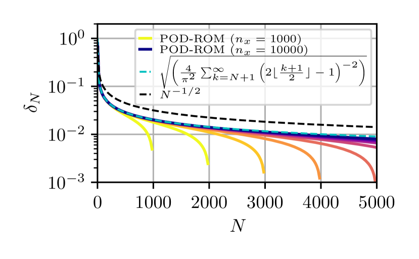
(a) POD vs. analytic error decay.

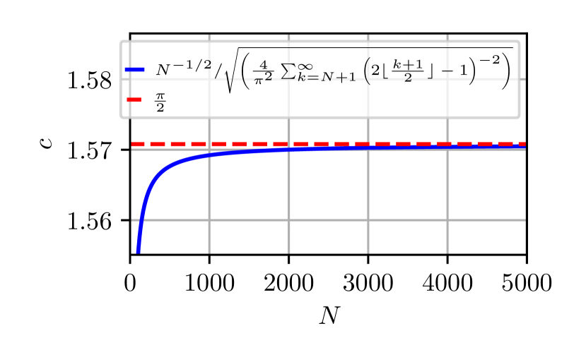
(b) Ratio of exact form to asymptotic rate.

Figure 1: Kolmorogov $N$-width $d_{N}({{\color[rgb]{0,0,0}\mathcal{U}_{g}}})$ for a discontinuous function – comparison of POD, exact form of $d_{N}({{\color[rgb]{0,0,0}\mathcal{U}_{g}}})$ and known asymptotic rate.

7.3 Smooth steep functions

We are now considering smooth functions which are “close” to a jump in the sense that they have one or more steep ramps. To this end, we construct an odd half-wave symmetric function, shown in Figure 2(b). The starting point is some smooth odd-symmetric function $q$ on the interval $(-\tfrac{1}{2},\tfrac{1}{2})$ (see Figure 2(a)). Based upon this, we define the odd HWS function $g=g_{q}$ by

$$g(x):=\begin{cases}1-2q(x+1),&-1<x\leq-\tfrac{1}{2},\\ 2q(x)-1,&-\tfrac{1}{2}<x\leq\tfrac{1}{2},\\ 1-2q(x-1),&\tfrac{1}{2}<x<1.\\ \end{cases}$$ (7.1)

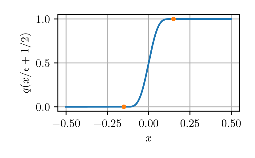
(a) Smooth function $q_{5}:(-\tfrac{1}{2},\tfrac{1}{2})\to\mathbb{R}$,
$x=\pm\varepsilon/2$ marked in orange.

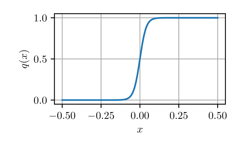
(b) Resulting odd HWS $g=g_{q}$ with junctions at dashed lines.

Figure 2: Construction of an odd HWS initial condition from a smooth ramp.

Following this idea, we can derive functions with arbitrary smoothness and arbitrarily steep ramps in order to be able to numerically investigate the dependence of the decay rate of $d_{N}({{\color[rgb]{0,0,0}\mathcal{U}_{g}}})$ on the regularity and the shape of the function. To this end, we construct a whole family $\{q_{m}\}_{m\in\mathbb{N}_{0}}$ such that $q_{m}\in C^{m}$ but $q_{m}\not\in C^{sm+1}$ (so that $m$ is the exact degree of regularity of $q_{m}$). We show an example of such functions $q_{0},...,q_{5}$ in (7.2). Starting from a linear function $q_{0}$, we successively increase the polynomial degree. A parameter $\varepsilon$ is used to control the steepness of the ramp. Then, we get

$$q_{0}(x/\varepsilon+1/2) :=x,$$ (7.2a)

$$q_{1}(x/\varepsilon+1/2) :=-2x^{3}+3x^{2},$$ (7.2b)

$$q_{2}(x/\varepsilon+1/2) :=6x^{5}-15x^{4}+10x^{3},$$ (7.2c)

$$q_{3}(x/\varepsilon+1/2) :=-20x^{7}+70x^{6}-84x^{5}+35x^{4},$$ (7.2d)

$$q_{4}(x/\varepsilon+1/2) :=70x^{9}-315x^{8}+540x^{7}-420x^{6}+126x^{5},$$ (7.2e)

$$q_{5}(x/\varepsilon+1/2) :=-252x^{11}+1386x^{10}-3080x^{9}+3465x^{8}-1980x^{7}+462x^{6},$$ (7.2f)

with the ramp being between $x=-\varepsilon/2$ and $x=\varepsilon/2$, the junctions are marked in Figure 2(a). Outside the ramp, $q_{m}\equiv 0$ and $q_{m}\equiv 1$ respectively. As an example of a $C^{\infty}$-function, we use the sigmoid function $q_{\infty,5}$ defined recursively as $q_{\infty,k+1}(x):=\sin\left(\tfrac{\pi}{2}q_{\infty,k}(x)\right)$ with $q_{\infty,0}(x):=\frac{2(x-\mu)}{\varepsilon m}$, $m=\tfrac{\pi^{k}}{2^{k}}$ with the smooth limit $q_{\infty}$ having the property $q_{\infty}\equiv-1$ for $x<\mu-m\tfrac{\varepsilon}{2}$ as well as $q_{\infty}\equiv 1$ for $x>\mu+m\tfrac{\varepsilon}{2}$. We can continue this process to obtain a $C^{\infty}$-function, but do not go into details. In order to get a meaningful comparison for the dependency of the $N$-width in terms of smoothness, we will use $\varepsilon$ for such a fine-tuning. The aim is that all functions $q_{m}$ should feature a similar steep jump from $0$ to $1$, but differ in their regularity, which of course causes different shapes of the functions, see Figure 3. Hence, we fit each resulting $g_{q_{m}}$ to $g_{q_{0}}$ and choose $\varepsilon$ as the parameter resulting in the best fit. We indicate the resulting values for $\varepsilon$ in Table 1.

regularity	$C^{0}$	$C^{1}$	$C^{2}$	$C^{3}$	$C^{4}$	$C^{5}$
$\varepsilon$	0.025	0.03316	0.04002	0.04592	0.05116	0.05592

Table 1: Values for $\varepsilon$ for each $g_{m}$.

The resulting functions of different smoothness are plotted in Figure 3. As we can see from the left graph in Figure 3(a), the shape of all functions is quite similar. The main difference lies in the regularity as can be seen in the zoom in Figure 3(b).

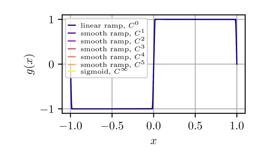
(a) Ramp functions on $\Omega_{\mathcal{P}}$.

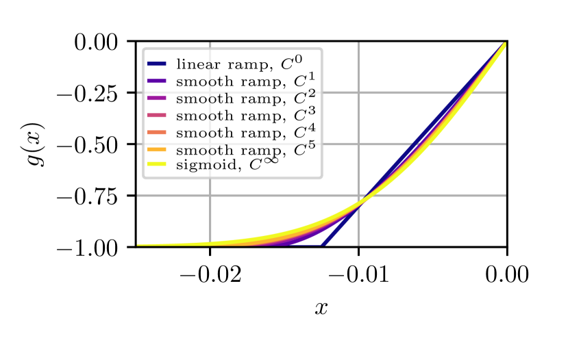
(b) Zoom into subinterval $[-0.025,0]$.

Figure 3: Ramp functions with varying smoothness $C^{m}$.

The results concerning the $N$-width are shown in Figure 4. On the left, in Figure 4(a), we compare the $N$-width $\delta_{N}({{\color[rgb]{0,0,0}\mathcal{U}_{g}}})$ for $g_{q_{{{\color[rgb]{0,0,0}m}}}}\in C^{m}(\Omega)$, $m=0,...,5$ and also for the $C^{\infty}$-sigmoid function (yellow) with exponential decay. We also indicate the error bound from Theorem 5.2, i.e., $\tilde{c}_{m}N^{-(m+1/2)}$. As there is no difference visible, in Figure 4(b), we plot the ratio of the numerically computed error and $c_{m}N^{-(m+1/2)}$ for a fitted $c_{m}$ for $m=0,...,5$. We see very good matches indicating that our bounds are sharp regarding $N$, in particular since the displayed functions are expected to have the Sobolev regularity $r(m)=m+1/2-\varepsilon$, see Corollary 5.3. As with the decay of the jump discontinuity (c.f. Figure 1(a)), the numerically computed decay for $N$ close to $\min(n_{x},n_{\mu})$ suffers from inaccuracies that are related to the discretization error.

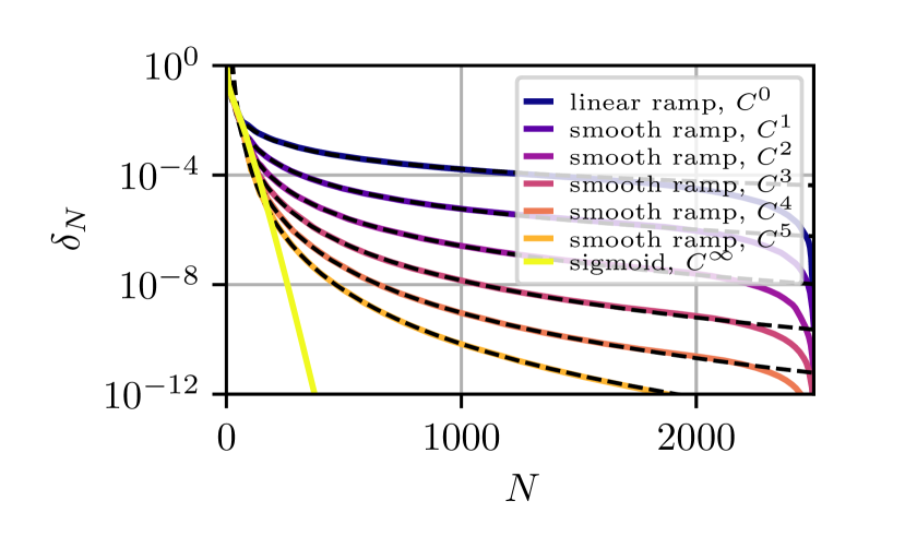
(a) $\delta_{N}$ and error estimation for $C^{m-1}$-functions.

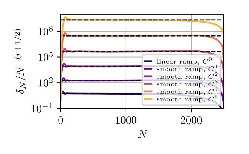
(b) Estimation of $c_{r}$ s.t. $\delta_{N}\approx c_{m}N^{-(m+1/2)}$.

Figure 4: $N$-width for ramps with varying regularity.

7.4 The impact of the slope

In §7.3 we have investigated functions with an almost identical ramp but with different smoothness. Now, we fix the regularity and vary the slope, i.e., the maximal value of the derivative (or norm of the gradient in higher dimensions). From our theoretical findings, we expect that the asymptotic decay rate should not be influenced by the slope. However, all estimates involve a multiplicative factor, which might depend on the slope. In order to clarify this, we consider a continuous, piecewise linear function with varying steepness. We choose the function $q_{0}$ in (7.2a) for different values of $\varepsilon$, see Figure 5(a). The results are displayed in Figure 5. We observe that the asymptotic rate is in fact identical, but the multiplicative factor grows when $\varepsilon$ decreases: the steeper the slope, the larger the $N$-widths.

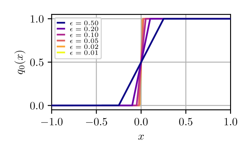
(a) Function $q_{0}$ for different $\varepsilon$.

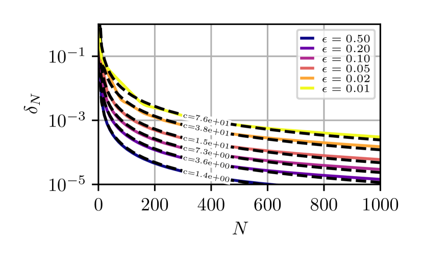
(b) $\delta_{N}({{\color[rgb]{0,0,0}\mathcal{U}_{g}}})$ for different $\varepsilon$.

Figure 5: $N$-width depending on the slope of a continuous, piecewise linear function.

7.5 Beyond symmetry

Finally, we consider almost arbitrary functions $g$ to define initial and boundary conditions for our original linear transport problem (2.1) in the sense that $g_{|[-1,0]}$ defines the inflow (i.e., the boundary condition) and $g_{|[0,1]}$ is the initial condition on $\Omega$. Again, we focus on the influence of the regularity on the decay of the $N$-width. To this end, we start by a piecewise constant discontinuous function as displayed in Figure 6(a) (dark blue), where the height of the $20$ steps are chosen at random. Smother versions are constructed by applying a convolution with a uniform box kernel, that is as wide as the distance between two discontinuities, see also Figure 6(a). The $N$-width is shown in Figure 6(b), where $-$again$-$ we clearly see the dependence of the decay on the regularity; the smoother the function, the better the rate. The rates are the same as in the previous case, but the constants (indicated in Figure 6(b)) differ. This experiment confirms our results also beyond half-wave symmetry, which we had to assume for the given proofs.

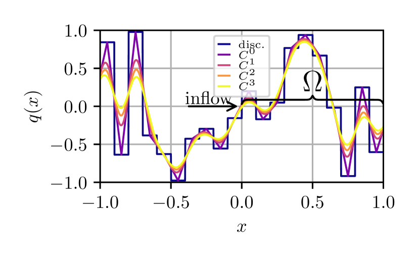
(a) Piecewise constant with $20$ random steps (dark blue); increasing smoothness $C^{m}(\Omega_{\mathcal{P}})$ by $m+1$-fold convolution, $m=0,...,3$.

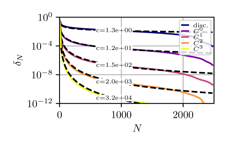
(b) $N$-width decay for discontinuous function and $g\in C^{m}(\Omega_{\mathcal{P}})$, $m=0,...,3$.

Figure 6: $\delta_{N}({{\color[rgb]{0,0,0}\mathcal{U}_{g}}})$ for random functions of different smoothness.

A 2D-example

All our analysis above was restricted to the 1D case $\Omega=(0,1)$. However, from the presentation it should be clear that at least some of what has been presented can be generalized to the higher-dimensional case by means of tensor products. In order to show this also numerically, we consider a linear transport problem on $\Omega=(0,1)^{2}$, see Figure 7(a). Note, that the parameter $\mu$ remains univariate. There, we indicate piecewise constant boundary conditions (on the left square yielding the inflow conditions) and initial conditions on $\Omega$ (on the right square). As before, we realize initial and boundary conditions of higher regularity by applying convolutions. The resulting $N$-widths are displayed in Figure 7(b), where we see once more that the rate is correlated to the regularity.

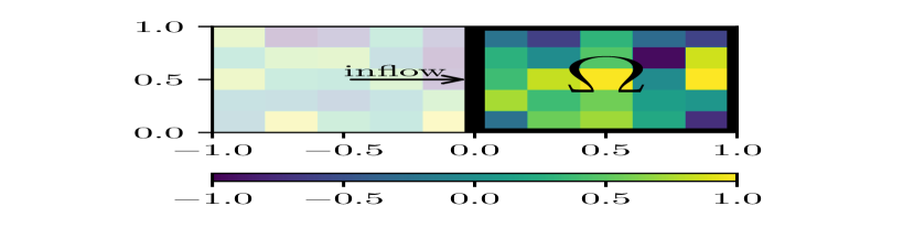
(a) Piecewise constant initial and boundary conditions indicated by color boxes.

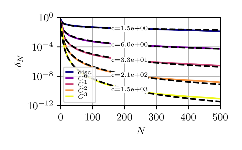
(b) Kolmorogov $N$-width for $C^{m}(\Omega_{\mathcal{P}})$-conditions, $m=0,...,{{\color[rgb]{0,0,0}3}}$.

Figure 7: 2D-transport problem: $\delta_{N}$-width for initial- and boundary conditions of different regularity $C^{m}(\Omega_{\mathcal{P}})$, $m=0,...,{{\color[rgb]{0,0,0}3}}$.

8 Conclusions

We have derived both exact representations as well as sharp bounds for the $N$-width for significant classes of functions used as initial and boundary values for the linear transport problem. The influence of the regularity on the decay has been rigorously investigated, namely $N^{-r}$ for functions in the Sobolev space $H^{r-\varepsilon}$. It became clear that a poor decay of the $N$-width is only a question of the smoothness of the solution in terms of the parameter, not of the problem itself. In other words, the decay does not necessarily depend on the PDE, but on the data such as initial and boundary values. We have also seen that the constant in the decay estimate depends on the slope of the function in a severe manner.

Our main tool is Fourier analysis and the notion of half-wave symmetric functions. This notion allowed us to construct linear spaces which we have shown to be optimal in the sense of Kolmogorov. Since any function can be written as a sum of even and odd HWS function, we derived a general upper estimate for the $N$-width. We have investigated both the $L_{2}(\mathcal{P})$-based $N$-width $\delta_{N}({{\color[rgb]{0,0,0}\mathcal{U}_{g}}})$ and the $L_{\infty}(\mathcal{P})$-based (worst case) $N$-width $d_{N}({{\color[rgb]{0,0,0}\mathcal{U}_{g}}})$ and we have proven $\delta_{N}({{\color[rgb]{0,0,0}\mathcal{U}_{g}}})=d_{N}({{\color[rgb]{0,0,0}\mathcal{U}_{g}}})$ for all HWS functions (Thm. 4.9). We conjecture that this upper bound is also asymptotically sharp, but we do not have a proof yet. Finally, the presented approach could also be generalized and adapted for other kinds of PPDEs.

Statements and Declarations

FA gratefully acknowledges STIPINST funding [318024] from the Research Council of Norway. The authors declare no competing interests.

References

- \bibcommenthead
- Kolmogorov [1936] Kolmogorov, A.: Über die beste Annäherung von Funktionen einer gegebenen Funktionenklasse. Annals of Mathematics 37(1), 107–110 (1936)
- Pinkus [1985] Pinkus, A.: N-Widths in Approximation Theory. Springer, Berlin (1985)
- DeVore [1998] DeVore, R.A.: Nonlinear approximation. Acta Numerica 7, 51–150 (1998)
- Floater et al. [2021] Floater, M.S., Manni, C., Sande, E., Speleers, H.: Best low-rank approximations and Kolmogorov -widths. SIAM J. Matrix Anal. Appl. 42(1), 330–350 (2021)
- Bressan et al. [2021] Bressan, A., Floater, M.S., Sande, E.: On best constants in L2 approximation. IMA J. Numer. Anal. 41(4), 2830–2840 (2021)
- Cohen et al. [2010] Cohen, A., DeVore, R., Schwab, C.: Convergence rates of best N-term Galerkin approximations for a class of elliptic sPDEs. Found. Comp. Math. 10(6), 615–646 (2010)
- Cohen and DeVore [2015] Cohen, A., DeVore, R.: Kolmogorov widths under holomorphic mappings. IMA J. Numer. Anal. 36(1), 1–12 (2015)
- Melenk [2000] Melenk, M.: On n-widths for elliptic problems. J. Math. Anal. Appl. 247(1), 272–289 (2000)
- Benner et al. [2017] Benner, P., Ohlberger, M., Cohen, A., Willcox, K.: Model Reduction and Approximation. Computational Science & Engineering. SIAM, Philadelphia (2017)
- Hesthaven et al. [2015] Hesthaven, J.S., Rozza, G., Stamm, B.: Certified Reduced Basis Methods for Parametrized Partial Differential Equations. Springer, Cham (2015)
- Quarteroni et al. [2015] Quarteroni, A., Manzoni, A., Negri, F.: Reduced Basis Methods for Partial Differential Equations: An Introduction. Springer, Cham (2015)
- Binev et al. [2011] Binev, P., Cohen, A., Dahmen, W., DeVore, R., Petrova, G., Wojtaszczyk, P.: Convergence Rates for Greedy Algorithms in Reduced Basis Methods. SIAM J. Math. Anal. 43(3), 1457–1472 (2011)
- Bachmayr and Cohen [2017] Bachmayr, M., Cohen, A.: Kolmogorov widths and low-rank approximations of parametric elliptic PDEs. Math. Comp. 86(304), 701–724 (2017)
- DeVore [2017] DeVore, R.A.: The Theoretical Foundation of Reduced Basis Methods. Computational Science & Engineering, pp. 137–168. SIAM, Philadelphia (2017)
- Maday et al. [2002] Maday, Y., Patera, A.T., Turinici, G.: A priori convergence theory for reduced-basis approximations of single-parameter elliptic partial differential equations. J. Sci. Comp. 17, 437–446 (2002)
- Maday [2006] Maday, Y.: Reduced basis method for the rapid and reliable solution of partial differential equations. In: Proceedings of ICM, Madrid, EMS (2006)
- Rozza et al. [2008] Rozza, G., Huynh, D.B.P., Patera, A.T.: Reduced basis approximation and a posteriori error estimation for affinely parametrized elliptic coercive partial differential equations: Application to transport and continuum mechanics. Arch. Comput. Methods Eng. 15(3), 229–275 (2008)
- Buffa et al. [2012] Buffa, A., Maday, Y., Patera, A.T., Prud’homme, C., Turinici, G.: A priori convergence of the greedy algorithm for the parametrized reduced basis method. ESAIM Math. Model. Numer. Anal. 46(3), 595–603 (2012)
- Lassila et al. [2013] Lassila, T., Manzoni, A., Quarteroni, A., Rozza, G.: Generalized reduced basis methods and n-width estimates for the approximation of the solution manifold of parametric pdes. Boll. Un. Mat. Italiana 6(1), 113–135 (2013)
- Ohlberger and Rave [2016] Ohlberger, M., Rave, S.: Reduced basis methods: Success, limitations and future challenges. Proceedings of the Conference Algoritmy, 1–12 (2016)
- Maday et al. [2002a] Maday, Y., Patera, A.T., Turinici, G.: A priori convergence theory for reduced-basis approximations of single-parameter elliptic partial differential equations. J. Sci. Comp. 17(1), 437–446 (2002)
- Maday et al. [2002b] Maday, Y., Patera, A.T., Turinici, G.: Global a priori convergence theory for reduced-basis approximations of single-parameter symmetric coercive elliptic partial differential equations. C.R. Math. 335(3), 289–294 (2002)
- Greif and Urban [2019] Greif, C., Urban, K.: Decay of the Kolmogorov N-width for wave problems. Appl. Math. Lett. 96, 216–222 (2019)
- Arbes et al. [2022] Arbes, F., Jensen, Ø., Mardal, K.-A., Dokken, J.: Model order reduction of solidification problems. ECCOMAS Congress (2022)
- Attenborough [2003] Attenborough, M.P.: Mathematics for Electrical Engineering and Computing. Elsevier, Oxford (2003)
- Rudin [1987] Rudin, W.: Real and Complex Analysis, 3rd edn., p. 416. McGraw-Hill Book Co., New York (1987)