Dissipative Boundary State Preparation

Abstract

We devise a generic and experimentally accessible recipe to prepare boundary states of topological or non-topological quantum systems through an interplay between coherent Hamiltonian dynamics and local dissipation. Intuitively, our recipe harnesses the spatial structure of boundary states which vanish on sublattices where losses are suitably engineered. This yields unique non-trivial steady states that populate the targeted boundary states with infinite life times while all other states are exponentially damped in time. Remarkably, applying loss only at one boundary can yield a unique steady state localized at the very same boundary. We detail our construction and rigorously derive full Liouvillian spectra and dissipative gaps in the presence of a spectral mirror symmetry for a one-dimensional Su-Schrieffer-Heeger model and a two-dimensional Chern insulator. We outline how our recipe extends to generic non-interacting systems.

I Introduction

Dissipation is ubiquitous and traditionally seen as detrimental to quantum phenomena. Much effort is thus aimed at minimizing its effects. Recently, however, it has been realized that structured dissipation can instead lead to new and intriguing topological physics [1, 2, 3, 4, 5]. In the quantum realm, an example thereof are dynamical Liouvillian skin effects [6, 7, 8, 9] reflecting the underlying non-Hermitian (NH) topology [10, 11, 12, 13, 14] on the level of quantum master equations. Another exciting aspect is the preparation of topological steady states of matter through judiciously engineered dissipation, which provide an alternative to ground state cooling [1, 15, 16, 17, 18, 19, 20, 21, 22, 23]. A preeminent idea considers the limit of strong dissipation in which jump operators [24] mimic localized Wannier functions and facilitate a projection onto the pertinent (‘low energy’) subspace [1, 15, 16]. Yet, while conceptually appealing, such approaches are both extremely challenging to implement and face a number of fundamental obstructions [16, 17, 18].

Here, we consider an alternative approach that crucially depends on the interplay of both coherent dynamics and dissipation. This approach alleviates both practical and fundamental challenges: with directly accessible ingredients, we can devise a combination of Hamiltonian dynamics and dissipation whose interplay uniquely prepares the system in what is the key hallmark of a topological phase, namely its boundary states. At long times all bulk modes vanish and only the boundary states prevail. A minimal example is shown in Fig. 1. Adding loss on a single site in a Su-Schrieffer-Heeger (SSH) chain evolves the system into a state localized at the same boundary. Our recipe is generic and can be applied to essentially any topological (or non-topological) noninteracting system. It also does not rely on fine tuning. Instead, the success of the construction is rooted in choosing lattices harboring boundary modes with the unique property of being the only eigenstates that vanish exactly on some sublattices [25, 26, 27, 28]—where we engineer loss. In fact, in the SSH example of Fig. 1, the same boundary steady state is obtained whenever loss is applied to one or more of the B-sites.

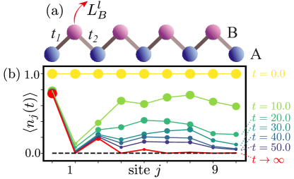
Figure 1: Minimal example: boundary state from single site loss. An open SSH chain with local loss only on the first site of the B sublattice (a), exhibiting a dynamical damping towards the boundary state at the same boundary (b) as indicated by the particle density $\left<n_{j}(t)\right>$ for a chain of length $L=2N-1=9$ with $t_{1}=0.5$, $t_{2}=1.0$ and $\gamma_{B}=0.5$.

We derive the aforementioned results analytically, and in the presence of a spectral mirror symmetry we obtain the full exact Liouvillian spectrum of the corresponding Lindblad master equation. We exemplify our construction for SSH chains with even and odd number of sites (Figs. 1-3) and for a two-dimensional (2D) Chern insulator hosting exact chiral edge steady states (Fig. 4). We also consider the effect of gain yielding steady state currents and how our exact solutions provide key intuitions for non-solvable systems (cf. Fig. 3).

II Setup and dissipative SSH models

We consider the Lindblad master equation [29, 24] which captures quantum dynamics of Markovian dissipative systems [30, 31, 32, 33, 34],

$$\frac{d\rho}{dt}=\hat{\mathcal{L}}\rho\coloneqq-i[\mathcal{H},\rho]+\sum_{\mu}(\hat{L}_{\mu}\rho\hat{L}_{\mu}^{\dagger}-\frac{1}{2}\{\hat{L}_{\mu}^{\dagger}\hat{L}_{\mu},\rho\}),$$ (1)

where $\rho$ is the density matrix of the system and $\mu$ denotes the summation over all types of jump operators.

As a minimal example, we study an SSH model of spinless fermions with an odd number of sites $L=2N-1$, with Hamiltonian $\mathcal{H}_{S}=\sum_{j=1}^{N-1}t_{1}a_{j,A}^{\dagger}a_{j,B}+t_{2}a_{j+1,A}^{\dagger}a_{j,B}+\text{H.c}$. We add local loss on the first B site: $\hat{L}^{l}_{1,B}=\sqrt{\gamma^{l}_{0,B}}a_{1,B}$ [see Fig. 1(a)]. Here, $a_{j,A}^{\dagger}(a_{j,B})$ are creation (annihilation) operators on the sublattice A(B) in the $j$th unit cell satisfying anticommutation relations: $\{a_{j,\alpha},a_{j^{\prime},\alpha^{\prime}}^{\dagger}\}=\delta_{j,j^{\prime}}\delta_{\alpha,\alpha^{\prime}}$. The quadratic Hamiltonian and linear Lindblad dissipators yield a quadratic Lindbladian diagonalizable in the third quantization approach [35, 36, 37]. The damping matrix $X$ which governs the dynamics can be mapped to a NH tight-binding Hamiltonian encoding information of both the original Hamiltonian and Lindblad dissipators (see Appendix A),

$$X=\frac{\gamma}{2}\times I_{L\times L}+iU\mathcal{H}_{\text{NH}}U^{-1},\ \mathcal{H}_{\text{NH}}=\mathcal{H}_{S}+i\Upsilon,$$ (2)

under a unitary transformation $U=\text{diag}\{1,i,1,i\dots,1\}$. For a single loss on the first $B$ site, $\gamma=\gamma_{B}=|\gamma_{0,B}^{l}|/2$, $I=\text{diag}\{1,1,0,\dots\}$ and $\Upsilon=\text{diag}\{\gamma/2,-\gamma/2,0,\dots,0\}$. The damping matrix $X=X_{c(d)}$ denotes the equal contribution from two Majorana fermions species: $a_{j,A}=\frac{1}{2}(c_{j,A}-id_{j,A}),a_{j,B}=\frac{1}{2}(d_{j,B}+ic_{j,B})$. It can also be decomposed into its eigenmodes: $X=\sum_{m}\beta_{m}|\psi_{Rm}\rangle\langle\psi_{Lm}|$ with $m$ the band index. The left and right eigenvectors satisfy the biorthogonal relations [38, 12, 39]: $\underline{\psi}^{*}_{L,m}\cdot\underline{\psi}_{R,m^{\prime}}=\delta_{m,m^{\prime}}$.

This decomposition enables us to derive dynamical observables by integrating the Lindblad master equation. The particle number $\langle n_{j}(t)\rangle=\text{Tr}[a_{j}^{\dagger}a_{j}\rho(t)]$ reads (see Appendix A)

$$\langle n_{j}(t)\rangle-\langle n_{j}\rangle_{s}$$ (3)

$$=\sum_{m,m^{\prime}}\sum_{l=1}^{L}e^{-(\beta_{m}+\beta^{*}_{m^{\prime}})t}\psi_{Lm^{\prime}}(j)\psi^{*}_{Rm^{\prime}}(l)\psi_{Rm}(l)\psi_{Lm}^{*}(j),$$

where $\langle n_{j}\rangle_{s}=\langle n_{j}(t=\infty)\rangle=0$ corresponds to the trivial non-equilibrium steady state (NESS) in the presence of loss, i.e. an empty chain, and the initial condition is chosen as a completely filled chain. The eigenvalues $\beta_{m}$ of the damping matrix coincide with the rapidity spectrum of the Liouvillian [35, 8]. Its real part encodes the decay rates of different modes towards the NESS and we define the dissipative gap $\Delta=2\min\{\text{Re}[\beta_{m}]\}\geq 0$.

For an odd number of sites, $\mathcal{H}_{S}$ hosts a zero-energy boundary mode fully suppressed on the $B$ sublattice [28]: $\mathcal{H}_{S}\underline{\psi}_{0}=E_{0}\underline{\psi}_{0}$, $E_{0}=0$ and

$$\underline{\psi}_{0}=\mathcal{N}(r,0,r^{2},0,\dots,0,r^{N})^{T},$$ (4)

with $r=-t_{1}/t_{2}$ the localization factor and $\mathcal{N}^{2}=(1-r^{2})/[r^{2}(1-r^{2N})]$ a normalization. For $|r|<1$ $(>1)$, the boundary mode is exponentially localized at the left (right) end of the chain. Intuitively, the frustrated nature of the boundary mode indicates its robustness against local loss on any B site. Indeed, with a single loss on the first $B$ site, we find a vanishing rapidity for this boundary mode: $X\underline{\psi}_{R0}=\beta_{0}\underline{\psi}_{R0}$, $X^{\dagger}\underline{\psi}_{L0}=\beta^{*}_{0}\underline{\psi}_{L0}$ where $\beta_{0}=0$ and $\underline{\psi}_{R0}=\underline{\psi}_{L0}=\underline{\psi}_{0}$ while all bulk modes have a finite dissipative gap. It implies that starting from all sites that are filled, through the dissipation the system always selects the boundary mode as the non-trivial steady state. For $t\to\infty$, the particle number becomes

$$\langle n_{j}\rangle_{s}=\frac{r^{j-1}-r^{j+1}}{1-r^{2N}}\>\>(j\>\mathrm{odd}),\quad\langle n_{j}\rangle_{s}=0\>\>(j\>\mathrm{even}).$$ (5)

To verify our observation, in Fig. 1(b), we calculate the time evolution of the particle number on individual sites by numerically diagonalizing the damping matrix. At sufficiently long times, the boundary mode (red line), with $|r|=|-t_{1}/t_{2}|=0.5$ and site occupation $\langle n_{j}\rangle_{s}$ predicted by Eq. (5), exponentially localizes ($|r|<1$) even when the single B-site loss is placed close to the same left end of the chain. We also observe that with single weak loss ($\gamma/2\leq\left||t_{1}|-|t_{2}|\right|$), the bulk dissipative gap is inversely proportional to the chain length: $\Delta_{\text{bulk}}\propto\gamma/N$. The single loss of our minimal model is particularly useful for small system size in modern experimental setups.

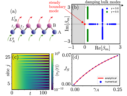
Figure 2: Solvable SSH chain with odd number of sites and uniform gain and loss. (a) Illustration of an open SSH chain with loss rate $\gamma_{B}$ on the B sublattice and gain rate $\gamma_{A}$ on the A sublattice. (b) Rapidity spectrum for $\gamma_{B}=0.5$ (green dots) and $\gamma_{B}=3.0$ (blue dots). The red dot at zero corresponds to the steady boundary mode. (c) Dynamics of the particle density $\left<n_{j}(t)\right>$ for a chain of length $L=2N-1=27$ with $t_{1}=2.0$, $t_{2}=1.0$, $\gamma_{A}=0.0$, $\gamma_{B}=0.5$. (d) Steady-state current $J_{S}$ as a function of $\gamma_{A}$. The other parameters are as in (c).

In the second example, while keeping the dissipationless feature of the boundary mode, we can make the dissipative gap of the bulk modes saturate in the large system size limit by adding loss on the entire B sublattice: $\hat{L}^{l}_{j,B}=\sqrt{\gamma^{l}_{0,B}}a_{j,B},\forall j$ [red arrows in Fig. 2 (a)]. The damping matrix $X$ in Eq. (2) holds new entries with $I=\mathbbm{1}_{L\times L}$ and $\Upsilon=(\gamma/2)\times\text{diag}\{1,-1,1,\dots,-1,1\}$. The rapidity for the boundary mode in Eq. (4) remains rigorously zero, $\beta_{0}=0$, and it is thus selected as the non-trivial steady state again. This steady boundary mode with a vanishing Liouvillian gap [denoted by the red dot in Fig. 2(b)] is not included in Ref. [40], while it is referred to as an ‘edge dark state’ in Ref. [41]. Remarkably, we can obtain the bulk dissipative gap analytically by exploiting spectral mirror symmetry under open boundary condition (OBC) with odd sites. The rapidity spectrum of the $(2N-2)$ bulk modes comes in pairs $\beta_{m}=\gamma/2\pm iE_{m}$, where $E_{m}$ denote the eigenenergies of $\mathcal{H}_{\text{NH}}$ from the mapping of Eq. (2) and we have adapted the notation for the band index $m=(\pm,q)$ with $q=\pi m^{\prime}/N$, $m^{\prime}=1,2,\dots,N-1$. The spectrum obeys spectral mirror symmetry $\beta^{{\text{OBC}}}_{\pm}(q)=\beta^{{\text{OBC}}}_{\pm}(-q)$, establishing a direct link to the spectrum under periodic boundary condition (PBC) [28, 39, 42]: $\beta^{\text{OBC}}_{\pm}(q)=\beta^{\text{PBC}}_{\pm}(q)$, reflecting the absence of a NH skin effect. We thus obtain $\beta_{\pm}^{\text{OBC}}(q)=\frac{\gamma}{2}\pm i\sqrt{t_{1}^{2}+t_{2}^{2}+2t_{1}t_{2}\cos(q)-\frac{\gamma^{2}}{4}}$. Shown in Fig. 2(b), all bulk modes have a finite gap and the minimum $\Delta_{\text{bulk}}=2\min\{\text{Re}[\beta_{\pm}(q)]\}$ determines the dissipative preparation time for the steady boundary mode: $\tau\sim\Delta_{\text{bulk}}^{-1}$. In the large-$N$ limit, we find the analytical solution to the bulk dissipative gap: $\Delta_{\text{bulk}}=\gamma$, for $\left||t_{1}|-|t_{2}|\right|\geq{\gamma}/2$; $\Delta_{\text{bulk}}=\gamma-\sqrt{\gamma^{2}-4(|t_{1}|-|t_{2}|)^{2}}$, otherwise. An exact complete set of right and left eigenvectors for the damping matrix $X$ is obtained as well (see Appendix A), where the bulk modes can be viewed as a superposition of two Bloch waves with opposite momenta vanishing on the last B site (which is removed in the odd chain). We are able to analytically resolve the full time evolution of the particle number shown in Fig. 2(c). For weak dissipation with $\Delta_{\text{bulk}}=\gamma$, the damping wavefront arises from the steady boundary mode, in contrast to previous studies with a major contribution from bulk skin modes [6, 7, 8, 9] (here our bulk modes are delocalized).

Next, we study the effect of small gain $\hat{L}^{g}_{j,A}=\sqrt{\gamma^{g}_{0,A}}a^{\dagger}_{j,A},\forall j$ on the A sublattice [green arrows in Fig. 2(a)]. The damping matrix $X$ in Eq. (2) is still exactly solvable with entries $\gamma=\gamma_{A}+\gamma_{B}$, $I=\mathbbm{1}_{L\times L}$, $\Upsilon=[(\gamma_{B}-\gamma_{A})/2]\times\text{diag}\{1,-1,1,-1,\dots,1\}$ and $\gamma_{A}=|\gamma^{g}_{0,A}|/2$. The boundary mode remains an eigenmode, yet it is associated with a non-zero rapidity $\beta_{0}=\gamma_{A}$ leading to a finite gap: $\Delta_{0}=2\gamma_{A}$. A small gain also eliminates the empty state as trivial NESS. In Appendix B, we identify the analytical structure of the non-trivial NESS in the presence of $\gamma_{A}$ as a mixed state continuously connected to the empty state and the boundary mode when $\gamma_{A}\to 0$. The system exhibits a steady state current $J_{S}=(i/L)\sum_{j}(\langle a_{j}^{\dagger}a_{j+1}\rangle_{s}-\langle a_{j+1}^{\dagger}a_{j}\rangle_{s})$, which we can obtain in a closed form [see Eq. 45]. We compare the analytical result with numerics in Fig. 2(d). Once $0<\gamma_{A}\ll\gamma_{B}$, regardless of the initial conditions, the system eventually evolves to the non-trivial NESS with a localization structure approximating the boundary mode in Eq. (4).

Figure 3: Topology and scaling in SSH chains with even number of sites and uniform loss. (a) Dynamics of the density $\left<n_{j}(t)\right>$ for a topologically trivial chain of length $L=2N=28$ with $t_{1}=2.0$, $t_{2}=1.0$, $\gamma_{B}=0.5$. (b) Dynamics of the density $\left<n_{j}(t)\right>$ for a topological chain of length $L=28$ with $t_{1}=0.5$, $t_{2}=1.0$, $\gamma_{B}=0.5$. (c) Real part of the rapidity spectrum as a function of $t_{1}$ for a system with $L=46$ sites and $t_{2}=1.0$, $\gamma_{B}=1.0$. (d) Dependence of the Liouvillian gap $\Delta=2\min\{\text{Re}[\beta_{m}]\}$ on the chain length $L$ for an even number of sites. Blue dots are the numerical result, while the red line indicates an exponential fit $f(N)=C\exp(-\alpha N)$ with $C=1.202$ and $\alpha=0.695$.

We now address the non-solvable model by obtaining the eigenmodes of the damping matrix through exact diagonalization (ED). The simplest scenario is encountered when we consider the SSH chain with an even number of sites $L=2N$. For $L=2N-1$, the model is symmetric under the exchange of $t_{1}$ and $t_{2}$ bonds [see Fig. 2(a)]. The boundary mode remains the steady state in both the topological ($|t_{1}|<|t_{2}|$) and non-topological ($|t_{1}|>|t_{2}|$) regions, with the localization direction reversed under the exchange ($|r|\to|r|^{-1}$). For $L=2N$, topology comes into play. With loss on the B sublattice, the boundary mode disappears in the topologically trivial region ($|t_{1}|>|t_{2}|$), as seen by comparing Fig. 3(a) with Fig. 2(c). Yet, it is retrieved in the topological region ($|t_{1}|<|t_{2}|$) [see Fig. 3(b)] with the same localization factor $|r|=|t_{1}/t_{2}|<1$ as in Eq. 4. This phenomenon can be predicted by noticing that two zero-energy boundary modes of the SSH model of even lengths are localized at different ends, and only one of them is protected under the B-sublattice loss [43, 44]. From the rapidity spectrum in Fig. 3(c), we observe this boundary mode only at $|t_{1}|<|t_{2}|$ and find that its dissipative gap decays exponentially with the chain length [see Fig. 3(d)]. The lifetime of the topological boundary state is enhanced exponentially by increasing the system size: $\tau\sim\Delta^{-1}\sim\exp{(\alpha N)}$ with $\alpha>0$, a remarkable feature due to topological protection.

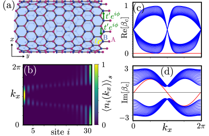
Figure 4: Preparation of chiral Chern insulator edge states. (a) Chern insulator on a cylinder geometry with (b) the distribution of the steady chiral mode prepared by B-sublattice loss as a function of $k_{x}$ along the $y$ direction. We adopt $L_{y}=2N-1=31$ for OBC and $L_{x}=200$ for PBC. The chiral edge state is localized at the left (right) boundary when $|r(k_{x})|=|2\cos(k_{x}/2)|<1$ ($>1$). The localization position changes at $k^{*}_{x}=2\pi/3,4\pi/3$ when $|r(k^{*}_{x})|=1$. (c),(d) Complex rapidity spectrum of the Chern insulator for $N=16$ and $t^{\prime}/t=\sqrt{3}/2$, $t=\gamma=1$ demonstrating bulk modes (blue lines) and exact chiral mode (red line). The real part (c) illustrates the dissipative gap and the imaginary part (d) is equivalent to the full energy spectrum.

III Generalization to dissipative lattice models in any dimension

Our recipe for devising unique steady boundary states naturally generalizes to any dimension with localization on boundaries of any co-dimension including surfaces, corners, edges and hinges. This is achieved by inferring results on boundary state solutions that vanish exactly on certain sublattices [26, 27]. In presence of a spectral mirror symmetry the full Liouvillian spectrum may be obtained [28]. Increasing both the bulk dimension and the codimension simultaneously is straightforward, yielding e.g. corner steady states on the breathing kagome lattice [45, 26], in full analogy with the SSH chain. Increasing the bulk dimension is suitably done by dimensional extension which is slightly more technically involved. Here, we provide an explicit example of dimensional extension in the preparation of dissipationless chiral edge modes of a two-dimensional Chern insulator on the honeycomb lattice [46, 28].

Figure 4(a) illustrates the corresponding cylinder geometry: we impose PBC on the $x$ direction with an even number of sites $L_{x}$ and OBC along the $y$ direction with an odd number of sites $L_{y}=2N-1$. The real nearest-neighbor and next-nearest-neighbor hopping amplitudes are denoted as $t$ and $t^{\prime}$. The complex hoppings $t^{\prime}e^{i\phi}$ with $\phi=\pi/2$ are allowed only between unit cells along the $x$ direction. For each $k_{x}$, a mapping to the generic SSH-like model can be established (see Appendix C): $\mathcal{H}_{S}(k_{x})=\sum_{j}\sum_{\alpha=A,B}\epsilon_{\alpha}a_{j,\alpha}^{\dagger}a_{j,\alpha}+\sum_{j=1}^{N-1}t_{1}a_{j,A}^{\dagger}a_{j,B}+t_{2}a_{j+1,A}^{\dagger}a_{j,B}+\text{H.c.}$, with $t_{1}=2t\cos(k_{x}/2),t_{2}=t,\epsilon_{A}=-\epsilon_{B}=-2t^{\prime}\sin(k_{x})$ (we use renormalized $k_{x}=\sqrt{3}k_{x,0}$ compared with the actual value). With the $B$-sublattice loss $\gamma=\gamma_{B}$, the rapidity spectrum consists of two copies ($\mu=\pm 1$) for distinct Majorana fermions species ($c$, $d$). For the topological chiral mode, $\beta_{0}^{\mu}=-i\mu\epsilon_{A}$ while for the bulk modes, the spectral mirror symmetry $\beta_{\pm}^{{\mu}}(k_{x},k_{y})=\beta_{\pm}^{{\mu}}(k_{x},-k_{y})$ leads to $\beta_{{\mu},\pm}^{\text{OBC}}(k_{x},k_{y})=\beta_{{\mu},\pm}^{\text{PBC}}(k_{x},k_{y})={\gamma}/{2}\pm i\sqrt{t_{1}^{2}+t_{2}^{2}+2t_{1}t_{2}\cos(k_{y})+(i\gamma/2-\mu\epsilon_{A})^{2}}$ with $k_{y}=\pi j/N$, $j=1,\dots,N-1$. Figures 4(c) and 4(d) show the real and imaginary parts of the rapidity spectrum of the chiral mode (red) and bulk modes (blue). The bulk modes have a vanishing dissipative gap in the large system limit at the momenta $k^{*}_{x}$ which satisfies $|r(k^{*}_{x})|=1$ where the chiral mode becomes delocalized and switches sides. Nevertheless for momenta when the chiral mode is isolated within the real rapidity spectrum of Fig. 4(c), the system has a finite instantaneous $\Delta_{\text{bulk}}$ to separate the chiral and bulk modes for any system size, and thus inherits the localization structure to the boundary mode of the SSH model with $|r(k_{x})|=|t_{1}/t_{2}|=|2\cos(k_{x}/2)|$. This feature is illustrated by the steady state particle number of Eq. (5) in Fig. 4(b).

IV Discussion

In this work, we have explored an alternative to ground state cooling and Floquet engineering of topological phenomena [47, 48, 17, 49, 50, 51], as well as other finite-time methods to probe boundary states [52, 53]. Our generic approach utilizes both dissipation and coherent dynamics to prepare boundary states as steady states which can be operated at arbitrarily long times. It circumvents the problem of thermal excitations faced at finite temperature in existing platforms. Compared with other dissipative preparation schemes [1, 15], in our recipe coherent dynamics from the Hamiltonian itself is introduced, while the form of dissipation is greatly simplified.

Our exact construction is not only simple, but also very general. By choosing appropriate lattice geometries it carries over directly to a plethora of topological and non-topological boundary states, including Fermi arcs and higher-order states at corners and hinges which all have the desired nodal boundary state structure [25, 26, 27, 28]. Going beyond the idealized model, one can break spectral mirror symmetry in the SSH Hamiltonians by adding disorder on the nearest-neighbor hopping terms. We find that the unique localization structure of the boundary mode is a generic property of any odd length chain: it still vanishes on the entire B sublattice without its dissipative gap opening, and is robust against onsite-potential disorder on any B site (see Appendix D). In real experiments, weak disorder on the other sublattice and further-neighour interactions directly interfere with the boundary mode and should be precisely controlled. The latter can be effectively suppressed on sufficiently deep optical lattices [54] that make the SSH models applicable [55, 56, 57, 53].

From the theoretical side, our analytical study offers promising outlooks for future exploration as well. One could test targeted boundary state distillation in open systems inherent with Liouvillian skin effects [6, 7, 8, 9], critical phenomena [58, 59] and phase transitions [60, 61, 62]. In particular, the preparation of steady boundary modes with NH skin effects would bestow exponentially enhanced sensitivity on quantum sensing devices [63, 64, 65, 66, 67]. It is equally exciting to extend the current framework from open fermions to bosonic and even hybrid systems via a similar third quantization approach [68, 69, 70].

Very recently, experiments on light in lossy optical waveguides showed that a similar boundary state preparation is possible at the level of NH effective Hamiltonians in classical settings [43]. The present work shows that a similar NH phenomenology is also relevant in the quantum realm and opens up different avenues for quantum control.

We also note that related systems with staggered loss or weak measurements have been considered earlier in the context of quantum walks described by effective NH Hamiltonians [71, 72, 73]. There, however, rather than the preparation of topological boundary states the focus was on other aspects such as defects, phase transitions and mean displacement.

Recently, we became aware of two independent works numerically observing the amplification of states at one boundary in Chern insulator models with gain and loss [41, 74]. In these studies, the boundary modes are classified and dynamically selected [43, 75, 44] as long-lived modes on even-length lattice models, but not as steady states once the system size becomes finite. By contrast, our predominantly analytical work focuses on odd-length lattice models and achieves this goal with generic boundary states hosting an exact zero dissipative gap. We also consider systems in which the entire family of boundary states is prepared, such as the Chern insulator model. This indicates a great flexibility and generality in harnessing structured dissipation for probing topological boundary state physics through its interplay with coherent Hamiltonian dynamics.

Acknowledgements.– We thank Mohamed Bourennane, Johan Carlström, Sebastian Diehl, and Kohei Kawabata for discussions. This work was supported by the Swedish Research Council (Grant No. 2018-00313), the Knut and Alice Wallenberg Foundation (KAW) via the Wallenberg Academy Fellows program (Grant No. 2018.0460) and the project Dynamic Quantum Matter (Grant No. 2019.0068), as well as the Göran Gustafsson Foundation for Research in Natural Sciences and Medicine.

Appendix A Liouvillian spectrum of 1D SSH model at odd lengths

Here we present the exact solutions to the Lindblad master equation for the SSH model with loss on the $B$ sublattice at arbitrary odd number of sites using third quantization. The exactly solvable dissipationless boundary mode together with the damping bulk modes give us full access to the quantum dynamics of the relaxation process, as well as a non-trivial non-equilibrium steady state (NESS).

A.1 Derivation of the damping matrix in third quantization

We start by writing the Hamiltonian of an SSH chain of spinless fermions with an odd number of sites: $\mathcal{H}_{S}=\sum_{j=1}^{N-1}t_{1}a_{j,A}^{\dagger}a_{j,B}+t_{2}a_{j+1,A}^{\dagger}a_{j,B}+\text{H.c.}$. The operator $a_{j,A}^{\dagger}(a_{j,B})$ creates (annihilates) a fermion on the sublattice A(B) in the $j$-th unit cell and they satisfy fermionic anticommutation relations: $\{a_{j,\alpha},a_{j^{\prime},\alpha^{\prime}}^{\dagger}\}=\delta_{j,j^{\prime}}\delta_{\alpha,\alpha^{\prime}}$. The last unit cell is broken and the total number of sites becomes odd, $L=2N-1$. Adding particle loss on the $B$ sublattice with the jump operator $\hat{L}^{l}_{j,B}=\sqrt{\gamma^{l}_{0,B}}a_{j,B}$ yields a quadratic Lindbladian from the Lindblad master equation in Eq. (1), of which the rapidity spectrum can be obtained via third quantization [35, 36, 37]. We briefly review the approach and adopt the same Majorana representation as in Ref. [8]. One spinless fermion can be mapped to two Majorana fermions per site:

$$a_{j,A}=\frac{1}{2}(c_{j,A}-id_{j,A}),\ a_{j,B}=\frac{1}{2}(d_{j,B}+ic_{j,B}).$$ (6)

This particular choice of mapping decouples two sectors in the damping matrix belonging to different Majorana fermions species $c$ and $d$. Let us group them into a whole set under a vector notation $\underline{w}=(w_{1},w_{2},\dots,w_{2L})^{T}=(c_{1},\dots,c_{L},d_{1},\dots,d_{L})^{T}$. Majorana fermions are their own anti-particles as evinced by $w_{j}^{\dagger}=w_{j}$, and they obey anticommutation relations $\{w_{j},w_{k}\}=2\delta_{j,k}$ such that each Majorana fermion squares to one. The density matrix $\rho$ in the original Hilbert space of dimension $2^{L}\times 2^{L}$ is now embedded in the set of Majorana operators with the new form $P_{\underline{\alpha}}=w_{1}^{\alpha_{1}}w_{2}^{\alpha_{2}}\cdots w_{2L}^{\alpha_{2L}}$, where $\alpha_{j}\in\{0,1\}$. In the Majorana representation, the Hamiltonian and Lindblad dissipators take the form: $\mathcal{H}=\sum_{j,k}w_{j}H_{j,k}w_{k}$ and $M_{ij}=\sum_{\nu=g,l}(l^{\nu}_{i,\mu})^{T}(l^{\nu}_{\mu,j})^{*}$. More precisely,

$$\underline{w}^{T}H\underline{w} =\begin{pmatrix}\underline{c}^{T}&\underline{d}^{T}\end{pmatrix}\begin{pmatrix}H_{0}&0\\ 0&H_{0}\end{pmatrix}\begin{pmatrix}\underline{c}\\ \underline{d}\end{pmatrix},$$

$$\underline{w}^{T}M\underline{w} =\begin{pmatrix}\underline{c}^{T}&\underline{d}^{T}\end{pmatrix}\begin{pmatrix}M_{1}&iM_{2}\\ -iM_{2}&M_{1}\end{pmatrix}\begin{pmatrix}\underline{c}\\ \underline{d}\end{pmatrix},$$ (7)

where

$$H_{0} =\frac{i}{4}\begin{pmatrix}0&t_{1}&&&&&\\ -t_{1}&0&-t_{2}&&&&\\ &t_{2}&0&t_{1}&&&\\ &&&\ddots&&&\\ &&&&&0&-t_{2}\\ &&&&&t_{2}&0\end{pmatrix},$$

$$M_{1} =\frac{1}{2}\begin{pmatrix}\gamma_{A}&&&&&&\\ &\gamma_{B}&&&&&&\\ &&\gamma_{A}&&&&\\ &&&&\ddots&&\\ &&&&&\gamma_{B}&\\ &&&&&&\gamma_{A}\end{pmatrix},$$

$$M_{2} =M_{1}(\gamma_{\alpha}\rightarrow\eta_{\alpha}),\quad\alpha=A,B,$$ (8)

where $\gamma_{\alpha}$’s and $\eta_{\alpha}$’s stand for the sum and the imbalance of the most generic loss and gain dissipators on two sublattices

$$2\gamma_{\alpha}=|\gamma_{0,\alpha}^{l}|+|\gamma^{g}_{0,\alpha}|,\quad 2\eta_{\alpha}=|\gamma_{0,\alpha}^{l}|-|\gamma^{g}_{0,\alpha}|,$$

$$\text{ for }\hat{L}^{l}_{j,\alpha}=\sqrt{\gamma^{l}_{0,\alpha}}a_{j,\alpha},\ \hat{L}^{g}_{j,\alpha}=\sqrt{\gamma^{g}_{0,\alpha}}a_{j,\alpha}^{\dagger},\ \forall j.$$ (9)

Over the $2^{2L}$-dimensional Liouville space $\mathcal{K}$, we now define adjoint fermionic operators that annihilate and create Majorana fermions: $\varphi_{j}|P_{\underline{\alpha}}\rangle=\delta_{\alpha_{j},1}|w_{j}P_{\underline{\alpha}}\rangle$, $\varphi_{j}^{\dagger}|P_{\underline{\alpha}}\rangle=\delta_{\alpha_{j},0}|w_{j}P_{\underline{\alpha}}\rangle$, which obey $\{\varphi_{j},\varphi_{k}^{\dagger}\}=\delta_{j,k}$. Since the Fermi parity $\mathcal{P}_{F}=(-1)^{\sum_{j}\varphi_{j}^{\dagger}\varphi_{j}}$ is conserved, $[\hat{\mathcal{L}},\mathcal{P}_{F}]=0$ and $(\mathcal{P}_{F})^{2}=1$, we can represent the Liouvillian in the even parity sector $\mathcal{P}_{F}=+1$ as

$$\hat{\mathcal{L}}_{+}=\frac{1}{2}\begin{pmatrix}\underline{\varphi}^{\dagger}\cdot&\underline{\varphi}\cdot\end{pmatrix}\begin{pmatrix}-X^{\dagger}&iY\\ 0&X\end{pmatrix}\begin{pmatrix}\underline{\varphi}\\ \underline{\varphi}^{\dagger}\end{pmatrix}-A_{0},$$ (10)

with $X=-4iH+M+M^{T}$, $Y=-2i(M-M^{T})$, and $A_{0}=\frac{1}{2}\text{Tr}[X]$. In the chosen Majorana fermions representation in Eq. (6), the full damping matrix is decoupled in different Majorana fermions species. The diagonal and off-diagonal blocks read

$$X=\begin{pmatrix}X_{c}&0\\ 0&X_{d}\end{pmatrix},\quad Y=4\begin{pmatrix}0&M_{2}\\ -M_{2}&0\end{pmatrix},$$ (11)

with $X_{c}=X_{d}=-4iH_{0}+2M_{1}$. The upper-triangular form of $\hat{\mathcal{L}}_{+}$ indicates that the eigenvalues of the Liouvillian coincide with those of the damping matrix $X$ [35, 8]. After proper diagonalization, we are able to express the Liouvillian in terms of rapidities $\beta$ and normal master modes (NMMs) $b^{\prime}$, $b$:

$$\hat{\mathcal{L}}_{+}=-\sum_{m=1}^{L}\beta_{m}(b^{\prime}_{c,m}b_{c,m}+b^{\prime}_{d,m}b_{d,m}).$$ (12)

Here, $\beta_{m}=\beta_{c,m}=\beta_{d,m}$ with the band index $m$ and NMMs satisfy the anticommutation relations $\{b^{\prime}_{c,m},b_{c,l}\}=\{b^{\prime}_{d,m},b_{d,l}\}=\delta_{m,l}$.

Furthermore, we can map the damping matrix in the Liouvillian to the SSH Hamiltonian with additional non-Hermitian imbalanced chemical potential on the two sublattices. For the (uniform) loss on the B sublattice only, we arrive at

$$X_{c}=X_{d}=\frac{\gamma}{2}\times\mathbbm{1}_{L\times L}+iU\mathcal{H}_{\text{NH}}U^{-1},\quad\mathcal{H}_{\text{NH}}=\mathcal{H}_{S}+i\Upsilon,$$

$$\mathcal{H}_{S}=\begin{pmatrix}0&t_{1}&&&&\\ t_{1}&0&t_{2}&&&\\ &t_{2}&0&&&\\ &&&\ddots&&\\ &&&&0&t_{2}\\ &&&&t_{2}&0\end{pmatrix}_{L\times L},$$

$$\Upsilon=\frac{\gamma}{2}\begin{pmatrix}1&&&&&\\ &-1&&&&\\ &&1&&&\\ &&&\ddots&&\\ &&&&-1&\\ &&&&&1\end{pmatrix}_{L\times L},$$ (13)

with the unitary transformation $U=\text{diag}\{1,i,1,i,\dots,i,1\}$ and $\gamma=|\gamma_{0,B}^{l}|/2$. Therefore, the rapidity spectrum satisfies the relation

$$\beta_{m}=\frac{\gamma}{2}+iE_{m},$$ (14)

where $E_{m}$ denotes the eigenvalues of the matrix $\mathcal{H}_{\text{NH}}=\mathcal{H}_{S}+i\Upsilon$.

A.2 Boundary mode and full rapidity spectrum with spectral mirror symmetry

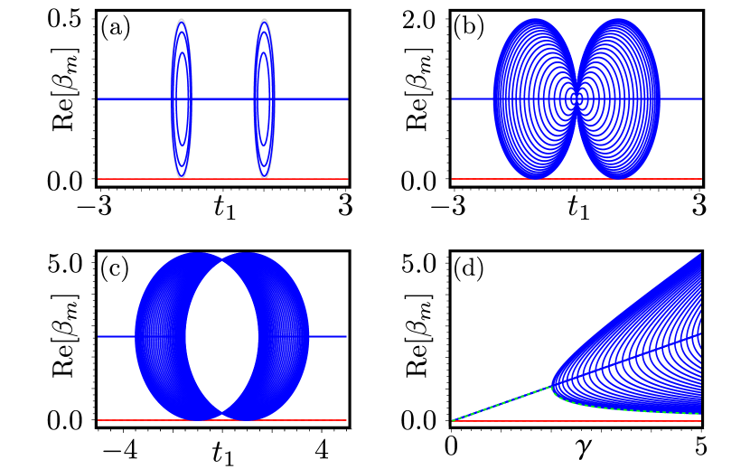
Figure 5: (a),(b) Real part of the rapidity spectrum as a function of $t_{1}$ for $t_{2}=1$ and $N=46$. The gray lines show the structure of the periodic system while the blue and red lines correspond to the bulk and boundary modes under OBC. We set different loss dissipation strengths on the B sublattice: (a) $\gamma=0.5$, (b) $\gamma=2$, (c) $\gamma=5$. (d) Real part of the rapidity spectrum as a function of $\gamma$ for $t_{1}=2$, $t_{2}=1$, and $N=46$. The green line denotes the half of the bulk dissipative gap estimated according to Eq. 20 for $N\gg 1$.

Under open boundary conditions (OBC), for the SSH chain with an odd number of sites $L=2N-1$, we first identify the zero-rapidity boundary mode $\beta_{m=0}=0$.

It comes from the zero-energy boundary state of the SSH Hamitonian:

$$\mathcal{H}_{S}\tilde{\underline{\psi}}_{m}=\tilde{E}_{m}\tilde{\underline{\psi}}_{m},\quad\tilde{E}_{0}=0,\ \tilde{\underline{\psi}}_{0}=\mathcal{N}\begin{pmatrix}r\\ 0\\ r^{2}\\ \cdots\\ 0\\ r^{N}\end{pmatrix},\ r=-\frac{t_{1}}{t_{2}},$$ (15)

where the normalization factor reads $\mathcal{N}^{2}=(1-r^{2})/[r^{2}(1-r^{2N})]$. It is straightforward to check that

$$(H_{\text{S}}+i\Upsilon)\tilde{\underline{\psi}}_{R0}=E_{0}\tilde{\underline{\psi}}_{R0},\quad E_{0}=i\frac{\gamma}{2},$$ (16)

which leads to zero rapidity from Eq. 14,

$$\beta_{0}=0,\quad\underline{\psi}_{R0}=\underline{\psi}_{L0}=\underline{\tilde{\psi}}_{0}.$$ (17)

Physically, this is consistent with the observation that the wave function of the zero-energy boundary mode is fully suppressed on the B sublattice for an SSH chain with an odd number of sites. The boundary mode survives under the dissipation on the frustrated sublattice in the infinitely long-time limit.

For a chain with an odd number of sites, the bulk spectrum fulfils a spectral mirror symmetry: $\beta_{\pm}^{\text{OBC}}(q)=\beta_{\pm}^{\text{OBC}}(-q)$. The mirror symmetry allows one to establish a rigorous relation between the spectrum under OBC and the spectrum under periodic boundary conditions (PBC)[28, 39, 42],

$$\beta_{\pm}^{\text{OBC}}(q) =\beta_{\pm}^{\text{PBC}}(q)$$

$$=\frac{\gamma}{2}\pm i\sqrt{t_{1}^{2}+t_{2}^{2}+2t_{1}t_{2}\cos(q)-\frac{\gamma^{2}}{4}},$$ (18)

with $q=\frac{\pi m^{\prime}}{N},\quad m^{\prime}=1,2,\dots,N-1$. We plot the real part of the rapidity spectrum as a function of the hopping amplitude and the dissipation strength in Fig. 5.

From the exact solutions, we can also obtain the dissipative gap that separates the boundary and bulk modes, together with the relaxation time $\tau$ for the system to evolve to the boundary mode in the long chain limit $N\gg 1$,

$${\Delta_{\text{bulk}}}=2\min\{\text{Re}[\beta_{m\neq 0}]\},\quad\tau\sim\frac{1}{\Delta},$$ (19)

where

$${\Delta_{\text{bulk}}}=\begin{cases}\gamma,&||t_{1}|-|t_{2}||\geq\gamma/2;\\ \gamma-\sqrt{\gamma^{2}-4(|t_{1}|-|t_{2}|)^{2}},&||t_{1}|-|t_{2}||<\gamma/2.\end{cases}$$ (20)

A.3 Exact eigenmodes of the damping matrix and dynamical observables

The complete set of eigenvectors of the damping matrix can be used to obtain dynamical observables. Apart from the exact boundary mode in Eq. (15), next we show how to construct the analytical solutions to the bulk eigenmodes.

To make the solutions more generic, we start from a Bloch form of the non-Hermitian tight-binding Hamiltonian $\mathcal{H}_{\text{NH}}$ into which the damping matrix can be transformed through Eq. (13),

$$\mathcal{H}_{\text{NH}}(q)=\vec{h}(q)\cdot\vec{\sigma},\quad\vec{h}=(h_{x},h_{y},h_{z}),\quad\vec{\sigma}=(\sigma_{x},\sigma_{y},\sigma_{z}),$$ (21)

where $h_{x},h_{y}\in\mathbb{R}$ and $h_{z}\in\mathbb{C}$. The non-Hermitian term enters into the sublattice potential. From the eigenvalue equations, $\mathcal{H}_{\text{NH}}\underline{u}_{R}(q)=E(q)\underline{u}_{R}(q)$ and $\mathcal{H}_{\text{NH}}^{\dagger}\underline{u}_{L}(q)=E^{*}(q)\underline{u}_{L}(q)$, one obtains the right and left eigenmodes of the Bloch Hamiltonian,

$$\underline{u}_{R,\pm}(q) =\frac{1}{\sqrt{2h(h{\mp}h_{z})}}\begin{pmatrix}h_{x}-ih_{y}\\ \pm h-h_{z}\end{pmatrix},$$

$$\underline{u}^{*}_{L,\pm}(q) =\frac{1}{\sqrt{2h(h{\mp}h_{z})}}\begin{pmatrix}h_{x}+ih_{y}\\ \pm h-h_{z}\end{pmatrix}.$$ (22)

Due to the spectral mirror symmetry, we establish the relation for energy eigenvalues switching from PBC to OBC,

$$E^{\text{OBC}}_{\pm}(q)=E^{\text{PBC}}_{\pm}(q)=\pm\sqrt{h_{x}^{2}+h_{y}^{2}+h_{z}^{2}},$$ (23)

with $q=\frac{\pi m^{\prime}}{N},\quad m^{\prime}=1,2,\dots,N-1$. Therefore, the bulk eigenmodes under OBC can be constructed as a superposition of the PBC eigenmodes at opposite momenta,

$$\underline{\tilde{\psi}}_{R/L,\nu}(q,j)=\frac{1}{\sqrt{2N}}\left(e^{iqj}\underline{u}_{R/L,\nu}(q)-e^{-iqj}\underline{u}_{R/L,\nu}(-q)\right).$$ (24)

Here, the minus sign is determined by the boundary condition, ensuring that the overall wavefunction vanishes on the B site of the last broken unit cell.

If we denote the band index as $m\in\{0,(\pm,q)\}$, it is straightforward to check that the boundary and bulk modes in Eqs. (15) and (24) satisfy the biorthogonal relations [38, 12, 39]: $\underline{\tilde{\psi}}^{*}_{L,m}\cdot\underline{\tilde{\psi}}_{R,l}=\delta_{m,l}$. The eigenmodes of the damping matrix can be obtained with an additional unitary transformation according to Eq. (13),

$$\underline{\psi}_{Rm}=U\ \tilde{\underline{\psi}}_{Rm},\quad\underline{\psi}_{Lm}=U\ \tilde{\underline{\psi}}_{Lm},$$ (25)

and they inherit the biorthogonal relations:

$${\underline{\psi}}_{Lm}^{*}\cdot{\underline{\psi}}_{Rl}=\tilde{\underline{\psi}}_{Lm}^{*}\cdot\tilde{\underline{\psi}}_{Rl}=\delta_{m,l}.$$ (26)

For the SSH model with loss on the B sublattice, we obtain the bulk modes by identifying

$$h_{x}=t_{1}+t_{2}\cos(q),\quad h_{y}=t_{2}\sin(q),\quad h_{z}=i\frac{\gamma}{2}.$$ (27)

It is then convenient to resolve the time evolution of the observables with the complete set of exactly solvable eigenstates of the damping matrix. Applying the anticommutation relations of Majorana fermions $\{w_{j},w_{k}\}=2\delta_{j,k}$ to the Lindblad master equation in Eq. 1, we arrive at the equation of motion for the covariance matrix $C_{jk}(t)=-\text{Tr}[w_{j}w_{k}\rho(t)]+\delta_{j,k}$:

$$\partial_{t}{C}(t)=-{C}(t)X-X^{\dagger}{C}(t)+iY.$$ (28)

For the trivial steady state,

$$\partial_{t}C_{s}=0,\quad C_{s}=i\begin{pmatrix}0&\mathbbm{1}_{L\times L}\\ -\mathbbm{1}_{L\times L}&0\end{pmatrix}.$$ (29)

Now, we define the expectation value of a local observable with respect to the trivial NESS: $\tilde{C}(t)=C(t)-C_{s}$. Starting from an arbitrary initial configuration that is not trivial $\tilde{C}(0)\neq 0$, we can integrate the equation of motion and implement the diagonalized damping matrix in the exponential,

$$X=\sum_{m}\sum_{\mu=c,d}\beta_{m}|\Theta^{\mu}_{Rm}\rangle\langle\Theta^{\mu}_{Lm}|,$$ (30)

$$|\Theta^{c}_{R(L)m}\rangle=\begin{pmatrix}\underline{\psi}_{R(L)m}\\ 0\end{pmatrix},\quad|\Theta^{d}_{R(L)m}\rangle=\begin{pmatrix}0\\ \underline{\psi}_{R(L)m}\end{pmatrix}.$$

Due to the biorthogonality of the basis, one reaches a compact form,

$$\tilde{C}(t)$$

$$=\sum_{m,m^{\prime}}\sum_{\mu,\mu^{\prime}}e^{-(\beta_{m}+\beta^{*}_{m^{\prime}})t}|\Theta^{\mu^{\prime}}_{Lm^{\prime}}\rangle\langle\Theta^{\mu^{\prime}}_{Rm^{\prime}}|\tilde{C}(0)|\Theta^{\mu}_{Rm}\rangle\langle\Theta^{\mu}_{Lm}|.$$ (31)

At $t=0$, we choose the system to be a completely filled chain: $\langle n_{j}(0)\rangle=1,\forall j$. It corresponds to a covariance matrix,

$$\tilde{C}(0)=-2i\begin{pmatrix}0&\mathbbm{1}_{n\times n}\\ -\mathbbm{1}_{n\times n}&0\end{pmatrix},$$ (32)

that selects $\mu\neq\mu^{\prime}$. Going back to the physical space consisting of spinless fermions, we define the single-particle correlator $Q_{jk}(t)=\text{Tr}[a_{j}^{\dagger}a_{k}\rho(t)]$. The mapping to Majorana fermions in Eq.( 6) yields

$$Q_{jk}(t)=\frac{i}{4}\sigma(j,k)\left[C_{j,{k+L}}(t)+C_{k,{j+L}}(t)\right],$$ (33)

where the phase factor depends on whether or not the correlation resides on the same sublattice,

$$\sigma(j,k)=\begin{cases}1,&j+k=\text{even};\\ (-1)^{j}\cdot(-i),&j+k=\text{odd}.\end{cases}$$ (34)

Combined with Eqs. 31 and 32, the single-particle correlator takes an explicit form in terms of the exact solutions of the damping matrix,

$$Q_{jk}(t)= \sigma(j,k)\sum_{m,m^{\prime}}\sum_{l=1}^{L}e^{-(\beta_{m}+\beta^{*}_{m^{\prime}})t}$$

$$\times\psi_{Lm}^{*}(j)\psi_{Lm^{\prime}}(k)\cdot\psi_{Rm}(l)\psi^{*}_{Rm^{\prime}}(l).$$ (35)

The particle number operator then reads

$$\langle\tilde{n}_{j}(t)\rangle=\langle n_{j}(t)\rangle-\langle n_{j}\rangle_{s}$$ (36)

$$=\sum_{m,m^{\prime}}\sum_{l=1}^{L}e^{-(\beta_{m}+\beta^{*}_{m^{\prime}})t}\psi_{Lm^{\prime}}(j)\psi^{*}_{Rm^{\prime}}(l)\psi_{Rm}(l)\psi_{Lm}^{*}(j),$$

where $\langle n_{j}\rangle_{s}=0$ denotes the trivial steady state.

Appendix B Non-equilibrium steady state for generic loss and gain

Below, we show the analytic structure of the non-trivial NESS with generic loss on the B sublattice and gain on the A sublattice. It also leads to a closed form for the steady state current.

Given the set of Lindblad dissipators $\hat{L}^{l}_{j,B}=\sqrt{\gamma^{l}_{0,B}}a_{j,B},\hat{L}^{g}_{j,A}=\sqrt{\gamma^{g}_{0,A}}a_{j,A}^{\dagger},\forall j$, the damping matrix from Eqs. (7)–(11) becomes

$$X_{c}=X_{d}=\frac{(\gamma_{A}+\gamma_{B})}{2}\times\mathbbm{1}_{L\times L}+iU(H_{\text{S}}+i\Upsilon)U^{-1},$$

$$\Upsilon=\frac{(\gamma_{B}-\gamma_{A})}{2}\begin{pmatrix}1&&&&&\\ &-1&&&&\\ &&1&&&\\ &&&\ddots&&\\ &&&&-1&\\ &&&&&1\end{pmatrix}_{L\times L},$$ (37)

with $\gamma_{A}=|\gamma_{0,A}^{g}|/2$ and $\gamma_{B}=|\gamma_{0,B}^{l}|/2$. The Bloch Hamiltonian of $\mathcal{H}_{\text{NH}}=\mathcal{H}_{S}+i\Upsilon=\vec{h}(q)\cdot\vec{\sigma}$ reads

$$h_{x}=t_{1}+t_{2}\cos(q),\quad h_{y}=t_{2}\sin(q),\quad h_{z}=i\frac{(\gamma_{B}-\gamma_{A})}{2}.$$ (38)

It encompasses all the ingredients to solving the rapidity spectrum,

$$\beta_{0} =\gamma_{A};$$ (39)

$$\beta_{\pm}(q) =\frac{\gamma_{A}+\gamma_{B}}{2}$$

$$\pm i\sqrt{t_{1}^{2}+t_{2}^{2}+2t_{1}t_{2}\cos(q)-\frac{(\gamma_{B}-\gamma_{A})^{2}}{4}},$$

together with the eigenmodes according to Eqs. (21)–(25).

To find the NESS that satisfies

$$\partial_{t}C_{s}=0,\quad X^{\dagger}C_{s}+C_{s}X=iY,$$ (40)

we begin by rewriting each matrix into the blocks,

$$X=\begin{pmatrix}X_{c}&0\\ 0&X_{d}\end{pmatrix},\quad C_{s}=\begin{pmatrix}0&D_{s}\\ -D_{s}&0\end{pmatrix},$$

$$Y=\begin{pmatrix}0&Y_{A}+Y_{B}\\ -(Y_{A}+Y_{B})&0\end{pmatrix}.$$ (41)

It simplifies to

$$X_{c}^{\dagger}D_{s}+D_{s}X_{c}=i(Y_{A}+Y_{B}),$$

$$Y_{A}=\begin{pmatrix}-2\gamma_{A}&&&&&\\ &0&&&&\\ &&-2\gamma_{A}&&&\\ &&&\ddots&&\\ &&&&0&\\ &&&&&-2\gamma_{A}\end{pmatrix},$$

$$Y_{B}=\begin{pmatrix}0&&&&&\\ &2\gamma_{B}&&&&\\ &&0&&&\\ &&&\ddots&&\\ &&&&2\gamma_{B}&\\ &&&&&0\end{pmatrix}.$$ (42)

In the presence of generic loss and gain, an analytical solution to the steady state covariance matrix follows

$$D_{s} =i(\mathbbm{1}_{L\times L}+\Delta D),$$ (43)

$$\Delta D =\sum_{m,m^{\prime}\neq 0}p_{m,m^{\prime}}|\underline{\psi}_{Lm}\rangle\langle\underline{\psi}_{Lm^{\prime}}|+c_{0}|\underline{\psi}_{L0}\rangle\langle\underline{\psi}_{L0}|.$$

While the matrix $\mathbbm{1}_{L\times L}$ in $D_{s}$ gives back the state of an empty chain due to loss, $c_{0}$ denotes the contribution from the boundary mode immune to loss and coefficients $p_{m,m^{\prime}}$ denote the overlaps between the bulk modes arising from gain,

$$c_{0}=p_{0,0}=-2,\quad p_{m,m^{\prime}}=\frac{\langle\psi_{Rm}|2Y_{A}|\psi_{Rm^{\prime}}\rangle}{\beta_{m}^{*}+\beta_{m^{\prime}}}.$$ (44)

We consider the scenario when $\gamma_{B}\gg\gamma_{A}$ and $\gamma_{A}\to 0^{+}$. The non-trivial NESS can be connected to a sum of the empty state and the boundary mode. Since the former gives zero particle number occupation, regardless of the initial conditions, the dissipative system always relaxes to a unique NESS with a localization structure approximating that of the boundary mode.

For the measurement of the steady-state current $J_{S}=(i/L)\sum_{j}(\langle a_{j}^{\dagger}a_{j+1}\rangle_{s}-\langle a_{j+1}^{\dagger}a_{j}\rangle_{s})$, we reach a closed form by substituting Eqs. (33) and (43) to the above definition:

$$J_{S}=-\frac{1}{L}\sum_{j}^{L-1}\sum_{m,m^{\prime}\neq 0}p_{m,m^{\prime}}\psi_{Lm}(j)\psi_{Lm^{\prime}}^{*}(j+1).$$ (45)

Appendix C Liouvillian spectrum of 2D Chern insulator

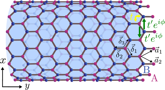
Figure 6: Illustration of a Chern insulator on a honeycomb lattice consisting of two sublattices A and B. We consider a system with PBC in the $x$ direction and OBC in the $y$ direction, yielding a cylinder geometry. We wrap the cylinder such that its edges are of zigzag type on the left and bearded type on the right. The vectors $\vec{a}_{1}$ and $\vec{a}_{2}$ indicate the Bravais lattice vectors of the honeycomb lattice, while $\vec{\delta}_{1}$ indicate the vectors in the three possible bond directions. The sites are coupled by nearest-neighbor hopping $t$ (depicted in yellow) and next-nearest-neighbor hopping $t^{\prime}$ (depicted in green). We further require that the next-nearest-neighbor hoppings along the $x$ direction acquire an additional phase factor $e^{i\phi}$ to open a Chern/Haldane insulator gap. In the text, we adopt $\phi=\pi/2$.

Here, we present more details on the derivation of the exactly solvable rapidity spectrum of a 2D dissipative Chern insulator [46, 28] through a mapping to the generic SSH model.

As shown in Fig. 6, we place the honeycomb lattice on a cylinder and adopt PBC along the $x$ direction with $M$ unit cells and OBC along the $y$ direction with $N$ unit cells. The last unit cell along the $y$ direction is broken, leading to $L_{y}=2N-1$ sites. We choose the zigzag edge on the left boundary and the bearded edge on the right boundary. The nearest-neighbor and next-nearest-neighbor hopping strengths are denoted by real parameters $t$ and $t^{\prime}$. The complex hoppings $t^{\prime}e^{i\phi}$ with $\phi=\pi/2$ are allowed only within unit cells along the $y$ direction. Setting the honeycomb lattice constant to $1$, different unit cells are connected by the vectors

$${\vec{a}_{1}=(\frac{\sqrt{3}}{2},\frac{3}{2}),\quad\vec{a}_{2}=(-\frac{\sqrt{3}}{2},\frac{3}{2}).}$$ (46)

First, we perform a Fourier transform on the $x$ components of the fermionic annihilation and creation operators ($\alpha=A,B$),

$$\vec{r}=(l,j),\quad a_{\alpha}(l,j)=\frac{1}{\sqrt{M}}\sum_{k_{x}}e^{ik_{x}l}a_{\alpha}(k_{x},j).$$ (47)

For each $k_{x}=2\pi m^{\prime}/M,m^{\prime}=-M/2,\dots,M/2-1$, the real-space Hamiltonian shares the form

$$H(k_{x})|_{L_{y}\times L_{y}}$$ (48)

$$=\begin{pmatrix}H_{A}&H_{A\leftarrow B}&&&&\\ H_{A\leftarrow B}^{\dagger}&H_{B}&H_{B\rightarrow A}^{\dagger}&&\\ &H_{B\rightarrow A}&H_{A}&&\\ &&&\ddots&&\\ &&&&{H_{B}}&{H_{B\rightarrow A}^{\dagger}}\\ &&&&{H_{B\rightarrow A}}&{H_{A}}\end{pmatrix}.$$

The matrix elements can be obtained as follows:

$$H_{A}: \sum_{l}t^{\prime}e^{i\phi}a_{A}^{\dagger}(l,j)a_{A}(l+\vec{a}_{1}-\vec{a}_{2},j)+\text{H.c.}$$

$$=\sum_{k_{x}}-2t^{\prime}\sin(k_{1}-k_{2})a_{A}^{\dagger}(k_{x},j)a_{A}(k_{x},j),$$

$$H_{B}: \sum_{l}t^{\prime}e^{-i\phi}a_{B}^{\dagger}(l,j)a_{B}(l+\vec{a}_{1}-\vec{a}_{2},j)+\text{H.c.}$$

$$=\sum_{k_{x}}2t^{\prime}\sin(k_{1}-k_{2})a_{B}^{\dagger}(k_{x},j)a_{B}(k_{x},j),$$

$$H_{A\leftarrow B}: \sum_{l}ta_{A}^{\dagger}(l,j)a_{B}(l,j)+ta_{A}^{\dagger}(l,j)a_{B}(l-(\vec{a}_{1}-\vec{a}_{2}),j)$$

$$=\sum_{k_{x}}t(1+e^{-i(k_{1}-k_{2})})a_{A}^{\dagger}(k_{x},j)a_{B}(k_{x},j),$$

$$H_{B\rightarrow A}: \sum_{l}ta_{A}^{\dagger}(l,j+1)a_{B}(l-1,j)$$

$$=\sum_{k_{x}}te^{-i(k_{1}-k_{2})/2}a_{A}^{\dagger}(k_{x},j+1)a_{B}(k_{x},j),$$ (49)

where $k_{i}=\vec{k}\cdot\vec{a}_{i}$, $i=1,2$.

Next, let us absorb the complex phases appearing in the hopping terms by the transformation

$$a_{A}(k_{x},j)\to e^{-i(k_{1}-k_{2})/2}a_{A}(k_{x},j).$$ (50)

It allows us to map $H(k_{x})$ to a generic SSH model with real hopping terms as before,

$$\mathcal{H}_{S}(k_{x}) =\sum_{j=1}^{N-1}t_{1}a_{j,A}^{\dagger}a_{j,B}+t_{2}a_{j+1,A}^{\dagger}a_{j,B}+\text{H.c.}$$

$$+\sum_{j}\sum_{\alpha=A,B}\epsilon_{\alpha}a_{j,\alpha}^{\dagger}a_{j,\alpha}$$ (51)

with $t_{1}=2t\cos(k_{x}/2),t_{2}=t,\epsilon_{A}=-\epsilon_{B}=-2t^{\prime}\sin(k_{x})$.

For simplicity, we have adopted the renormalized $k_{x}=k_{1}-k_{2}=\sqrt{3}k_{x,0}$, compared with the original value $k_{x,0}$ on the honeycomb lattice.

Adding the B sublattice loss $\hat{L}^{l}_{j,B}=\sqrt{\gamma^{l}_{0,B}}a_{j,B},\forall j$, we apply the Majorana fermions representation in Eq. 6. The generic SSH Hamiltonian reads

$$\underline{w}^{T}\mathcal{H}_{S}\underline{w}=\begin{pmatrix}\underline{c}^{T}&\underline{d}^{T}\end{pmatrix}\begin{pmatrix}H_{0}&-iH_{1}\\ iH_{1}&H_{0}\end{pmatrix}\begin{pmatrix}\underline{c}\\ \underline{d}\end{pmatrix},$$

$$H_{0}=\frac{i}{4}h_{0},\quad H_{1}=\frac{i}{4}h^{\prime},$$ (52)

where

$$h_{0} =\begin{pmatrix}0&t_{1}&&&&\\ -t_{1}&0&-t_{2}&&&\\ &t_{2}&0&&&\\ &&&\ddots&&\\ &&&&0&-t_{2}\\ &&&&t_{2}&0\end{pmatrix}_{L_{y}\times L_{y}},$$ (53)

$$h^{\prime} =\begin{pmatrix}-i\epsilon_{A}&&&&&\\ &-i\epsilon_{B}&&&&\\ &&-i\epsilon_{A}&&&\\ &&&\ddots&&\\ &&&&-i\epsilon_{B}&\\ &&&&&-i\epsilon_{A}\end{pmatrix}_{L_{y}\times L_{y}}.$$

And the damping matrix takes the form

$$X=\begin{pmatrix}\underline{c}^{T}&\underline{d}^{T}\end{pmatrix}\begin{pmatrix}h_{0}+2M_{1}&-ih^{\prime}\\ ih^{\prime}&h_{0}+2M_{1}\end{pmatrix}\begin{pmatrix}\underline{c}\\ \underline{d}\end{pmatrix},$$

$${M_{1}=\text{diag}\{0,\frac{\gamma}{2},0,\dots,\frac{\gamma}{2},0\},}$$ (54)

with $\gamma=\gamma_{B}=|\gamma_{0,B}^{l}|/2$. It is convenient to introduce a new set of Pauli matrices $\vec{\tau}$ acting on different subspaces of Majorana fermions species $c$ and $d$, in order to decouple them,

$$X=U_{0}\tilde{X}U_{0}^{-1},$$ (55)

$$\tilde{X}=\begin{pmatrix}h_{0}+h^{\prime}+2M_{1}&0\\ 0&h_{0}-h^{\prime}+2M_{1}\end{pmatrix}=\begin{pmatrix}\tilde{X}_{c}&0\\ 0&\tilde{X}_{d}\end{pmatrix},$$

where $U_{0}=(1+i\tau^{x})/\sqrt{2}$. The eigenmodes of $\tilde{X}_{c(d)}$ can be exactly solved by the method we have developed earlier in Eqs. (13)–(25), which requires the identification of their NH Bloch Hamiltonians in Eq. 21. From the mapping of the damping matrix in Eq. 13, one arrives at

$$h_{x}=t_{1}+t_{2}\cos({k_{y}}),\quad h_{y}=t_{2}\sin({k_{y}}),\quad h_{z}=i\frac{\gamma}{2}\mp\mu\epsilon_{A},$$ (56)

where $\mu=\pm 1$ for $c$, $d$, respectively. For the chiral edge mode,

$$\beta_{0}^{\mu}=-i\mu\epsilon_{A},\quad\underline{\psi}_{R0}=\underline{\psi}_{L0}=\mathcal{N}\begin{pmatrix}r\\ 0\\ r^{2}\\ \cdots\\ 0\\ r^{N}\end{pmatrix},$$

$$r(k_{x})=-\frac{t_{1}}{t_{2}}=-2\cos(k_{x}/2),$$ (57)

while for the bulk modes ($k_{y}=\pi m^{\prime}/N$ with $m^{\prime}=1,\dots,N-1$), the spectral mirror symmetry $\beta_{\pm}(k_{x},k_{y})=\beta_{\pm}(k_{x},-k_{y})$ leads to

$$\beta_{{\mu},\pm}^{\text{OBC}}(k_{x},k_{y})=\beta_{{\mu},\pm}^{\text{PBC}}(k_{x},k_{y})$$ (58)

$$={\gamma}/{2}\pm i\sqrt{t_{1}^{2}+t_{2}^{2}+2t_{1}t_{2}\cos(k_{y})+(i\gamma/2-\mu\epsilon_{A})^{2}}.$$

Furthermore, we check that the trivial steady state remains the same as the 1D SSH model (an empty state of spinless fermions along the $y$ direction),

$$C_{s}=i\begin{pmatrix}0&\mathbbm{1}\\ -\mathbbm{1}&0\end{pmatrix}.$$ (59)

The time evolution of the particle number distribution can be resolved as well,

$$\langle n_{j}(t)\rangle= \frac{1}{2}\sum_{m,m^{\prime}}\sum_{l=1}^{{L_{y}}}\sum_{\mu=c,d}e^{-(\beta_{\mu,m}+\beta^{*}_{\mu,m^{\prime}})t}$$ (60)

$$\times\psi_{L,\mu m^{\prime}}(j)\psi^{*}_{R,\mu m^{\prime}}(l)\psi_{R,\mu m}(l)\psi_{L,\mu m}^{*}(j).$$

Starting from a completely filled lattice driven by the B-sublattice loss, the steady-state particle number distribution becomes that of the chiral edge mode,

$$\langle n_{j}\rangle_{s}=\frac{r^{j-1}-r^{j+1}}{1-r^{2N}}\>\>(j\>\mathrm{odd}),\ \langle n_{j}\rangle_{s}=0\>\>(j\>\mathrm{even}).$$ (61)

Appendix D Robustness of the boundary state against sublattice and bond disorders

In the following, we discuss the robustness of the boundary state in Eq. 4 hosted by the 1D SSH model with odd sites, and generalize its localization structure in the presence of bond disorders.

Further-neighbor interactions and weak onsite-potential disorder on the A sublattice would eliminate the boundary mode from being a steady state of the Liouvillian. However, with loss engineering, there are other types of disorders that the boundary mode is robust against, including strong random disorders in the B-sublattice potentials and in the $t_{1}$ and $t_{2}$ hopping terms. Let us include them explicitly in the model with B-sublattice loss,

$$\mathcal{H}_{0}=\sum_{j=1}^{N-1}t_{j,1}a_{j,A}^{\dagger}a_{j,B}+t_{j,2}a_{j+1,A}^{\dagger}a_{j,B}+\text{H.c.},$$

$$V=\sum_{j}\omega_{j,B}a_{j,B}^{\dagger}a_{j,B},$$

$$\hat{L}^{l}_{j,B}=\sqrt{\gamma^{l}_{0,B}}a_{j,B},\forall j.$$ (62)

Casting the Hamiltonian into a matrix form, it is straightforward to check that due to local destructive interference arising from disordered nearest-neighbor hopping terms, the targeted zero-energy boundary state takes a new form,

$$H_{0}=\begin{pmatrix}0&t_{1,1}&&&&\\ t_{1,1}&0&t_{1,2}&&&\\ &t_{1,2}&0&t_{2,1}&&\\ &&&\ddots&&\\ &&&&0&t_{N-1,2}\\ &&&&t_{N-1,2}&0\end{pmatrix},$$

$$H_{0}\underline{\psi}_{0}=E_{0}\underline{\psi}_{0}:\ E_{0}=0,\ \underline{\psi}_{0}=\mathcal{N}(r_{1},0,r_{2},0,\dots,0,r_{N})^{T},$$

$$r_{1}=1,\quad r_{m}=\prod_{j=1}^{m-1}\left(-\frac{t_{j,1}}{t_{j,2}}\right),\ m>1,$$ (63)

with a normalization factor $\mathcal{N}^{-2}=\sum_{m=1}^{N}r_{m}^{2}$. It still shares a localization structure fully suppressed on the B sublattice, thus immune to both loss and on-site disorder on the same sublattice. Indeed, after a proper rotation in the subspaces of different Majorana fermions species $c$ and $d$ as has been performed in Eqs. (51)–(55), random on-site disorder acting as a real chemical potential enters the rotated damping matrix in the diagonal terms belonging to B sites and becomes purely imaginary ($\mu=+1,-1$ for $c,d$),

$$\tilde{X}_{c,d}= \begin{pmatrix}0&t_{1,1}&&&&\\ -t_{1,1}&0&-t_{1,2}&&&\\ &t_{1,2}&0&t_{2,1}&&\\ &&&\ddots&&\\ &&&&0&-t_{N-1,2}\\ &&&&t_{N-1,2}&0\end{pmatrix}$$

$$+\begin{pmatrix}0&&&&&&\\ &-i\mu\omega_{1,B}+\gamma_{B}&&&&&\\ &&0&&&&\\ &&&&\ddots&&\\ &&&&&-i\mu\omega_{N-1,B}+\gamma_{B}&\\ &&&&&&0\end{pmatrix}.$$ (64)

The vanishing gap of the generalized boundary mode ensures an infinite lifetime as a steady state,

$$\tilde{X}_{c,d}\underline{\psi}_{0}=\beta_{0}\underline{\psi}_{0},\quad\beta_{0}=0.$$ (65)

References

• Diehl et al. [2011] S. Diehl, E. Rico, M. A. Baranov, and P. Zoller, Topology by dissipation in atomic quantum wires, Nat. Phys. 7, 971 (2011).
• Gong et al. [2018] Z. Gong, Y. Ashida, K. Kawabata, K. Takasan, S. Higashikawa, and M. Ueda, Topological phases of non-Hermitian systems, Phys. Rev. X 8, 031079 (2018).
• Bergholtz et al. [2021] E. J. Bergholtz, J. C. Budich, and F. K. Kunst, Exceptional topology of non-Hermitian systems, Rev. Mod. Phys. 93, 015005 (2021).
• Miri and Alù [2019] M.-A. Miri and A. Alù, Exceptional points in optics and photonics, Science 363, eaar7709 (2019).
• Ashida et al. [2020] Y. Ashida, Z. Gong, and M. Ueda, Non-Hermitian physics, Advances in Physics 69, 249 (2020)https://doi.org/10.1080/00018732.2021.1876991 .
• Song et al. [2019] F. Song, S. Yao, and Z. Wang, Non-Hermitian skin effect and chiral damping in open quantum systems, Phys. Rev. Lett. 123, 170401 (2019).
• Haga et al. [2021] T. Haga, M. Nakagawa, R. Hamazaki, and M. Ueda, Liouvillian skin effect: Slowing down of relaxation processes without gap closing, Phys. Rev. Lett. 127, 070402 (2021).
• Yang et al. [2022] F. Yang, Q.-D. Jiang, and E. J. Bergholtz, Liouvillian skin effect in an exactly solvable model, Phys. Rev. Research 4, 023160 (2022).
• Kawabata et al. [2023] K. Kawabata, T. Numasawa, and S. Ryu, Entanglement phase transition induced by the non-Hermitian skin effect, Phys. Rev. X 13, 021007 (2023).
• Lee [2016] T. E. Lee, Anomalous edge state in a non-Hermitian lattice, Phys. Rev. Lett. 116, 133903 (2016).
• Yao and Wang [2018] S. Yao and Z. Wang, Edge states and topological invariants of non-Hermitian systems, Phys. Rev. Lett. 121, 086803 (2018).
• Kunst et al. [2018a] F. K. Kunst, E. Edvardsson, J. C. Budich, and E. J. Bergholtz, Biorthogonal bulk-boundary correspondence in non-Hermitian systems, Phys. Rev. Lett. 121, 026808 (2018a).
• [13] R. Lin, T. Tai, L. Li, and C. H. Lee, Topological non-Hermitian skin effect, arXiv:2302.03057 .
• Okuma and Sato [2023] N. Okuma and M. Sato, Non-Hermitian topological phenomena: A review, Annu. Rev. Condens. Matter Phys. 14, 83 (2023).
• Bardyn et al. [2013] C.-E. Bardyn, M. A. Baranov, C. V. Kraus, E. Rico, A. İmamoglu, P. Zoller, and S. Diehl, Topology by dissipation, New J. Phys. 15, 085001 (2013).
• Budich et al. [2015] J. C. Budich, P. Zoller, and S. Diehl, Dissipative preparation of Chern insulators, Phys. Rev. A 91, 042117 (2015).
• Goldman et al. [2016] N. Goldman, J. C. Budich, and P. Zoller, Topological quantum matter with ultracold gases in optical lattices, Nat. Phys. 12, 639 (2016).
• Goldstein [2019] M. Goldstein, Dissipation-induced topological insulators: A no-go theorem and a recipe, Sci. Phys. 7, 67 (2019).
• Shavit and Goldstein [2020] G. Shavit and M. Goldstein, Topology by dissipation: Transport properties, Phys. Rev. B 101, 125412 (2020).
• Tonielli et al. [2020] F. Tonielli, J. C. Budich, A. Altland, and S. Diehl, Topological field theory far from equilibrium, Phys. Rev. Lett. 124, 240404 (2020).
• Bandyopadhyay and Dutta [2020] S. Bandyopadhyay and A. Dutta, Dissipative preparation of many-body Floquet Chern insulators, Phys. Rev. B 102, 184302 (2020).
• Liu et al. [2021] Z. Liu, E. J. Bergholtz, and J. C. Budich, Dissipative preparation of fractional Chern insulators, Phys. Rev. Research 3, 043119 (2021).
• Vasiloiu et al. [2022] L. M. Vasiloiu, A. Tiwari, and J. H. Bardarson, Dephasing-enhanced Majorana zero modes in two-dimensional and three-dimensional higher-order topological superconductors, Phys. Rev. B 106, L060307 (2022).
• Lindblad [1976] G. Lindblad, On the generators of quantum dynamical semigroups, Commun. Math. Phys. 48, 119 (1976).
• Kunst et al. [2017] F. K. Kunst, M. Trescher, and E. J. Bergholtz, Anatomy of topological surface states: Exact solutions from destructive interference on frustrated lattices, Phys. Rev. B 96, 085443 (2017).
• Kunst et al. [2018b] F. K. Kunst, G. van Miert, and E. J. Bergholtz, Lattice models with exactly solvable topological hinge and corner states, Phys. Rev. B 97, 241405 (2018b).
• Kunst et al. [2019a] F. K. Kunst, G. van Miert, and E. J. Bergholtz, Boundaries of boundaries: A systematic approach to lattice models with solvable boundary states of arbitrary codimension, Phys. Rev. B 99, 085426 (2019a).
• Kunst et al. [2019b] F. K. Kunst, G. van Miert, and E. J. Bergholtz, Extended Bloch theorem for topological lattice models with open boundaries, Phys. Rev. B 99, 085427 (2019b).
• Breuer and Petruccione [2002] H.-P. Breuer and F. Petruccione, The theory of open quantum systems (Oxford University Press, New York, 2002).
• Diehl et al. [2008] S. Diehl, A. Micheli, A. Kantian, B. Kraus, H. Büchler, and P. Zoller, Quantum states and phases in driven open quantum systems with cold atoms, Nat. Phys. 4, 878 (2008).
• Kraus et al. [2008] B. Kraus, H. P. Büchler, S. Diehl, A. Kantian, A. Micheli, and P. Zoller, Preparation of entangled states by quantum Markov processes, Phys. Rev. A 78, 042307 (2008).
• Verstraete et al. [2009] F. Verstraete, M. M. Wolf, and J. I. Cirac, Quantum computation and quantum-state engineering driven by dissipation, Nat. Phys. 5, 633 (2009).
• Krauter et al. [2011] H. Krauter, C. A. Muschik, K. Jensen, W. Wasilewski, J. M. Petersen, J. I. Cirac, and E. S. Polzik, Entanglement generated by dissipation and steady state entanglement of two macroscopic objects, Phys. Rev. Lett. 107, 080503 (2011).
• Langen et al. [2015] T. Langen, R. Geiger, and J. Schmiedmayer, Ultracold atoms out of equilibrium, Annu. Rev. Condens. Matter Phys. 6, 201 (2015).
• Prosen [2008] T. Prosen, Third quantization: A general method to solve master equations for quadratic open Fermi systems, New J. Phys. 10, 043026 (2008).
• Prosen and Žunkovič [2010] T. Prosen and B. Žunkovič, Exact solution of Markovian master equations for quadratic Fermi systems: Thermal baths, open XY spin chains and non-equilibrium phase transition, New J. Phys. 12, 025016 (2010).
• Prosen [2010] T. Prosen, Spectral theorem for the Lindblad equation for quadratic open fermionic systems, J. Stat. Mech. 2010, P07020 (2010).
• Brody [2014] D. C. Brody, Biorthogonal quantum mechanics, J. Phys. A 47, 035305 (2014).
• Edvardsson et al. [2020] E. Edvardsson, F. K. Kunst, T. Yoshida, and E. J. Bergholtz, Phase transitions and generalized biorthogonal polarization in non-Hermitian systems, Phys. Rev. Research 2, 043046 (2020).
• Lieu et al. [2020] S. Lieu, M. McGinley, and N. R. Cooper, Tenfold way for quadratic Lindbladians, Phys. Rev. Lett. 124, 040401 (2020).
• Yang et al. [2023] F. Yang, Z. Wei, X. Tong, K. Cao, and S.-P. Kou, Symmetry classes of dissipative topological insulators with edge dark states, Phys. Rev. B 107, 165139 (2023).
• Edvardsson and Ardonne [2022] E. Edvardsson and E. Ardonne, Sensitivity of non-Hermitian systems, Phys. Rev. B 106, 115107 (2022).
• [43] W. Cherifi, J. Carlström, M. Bourennane, and E. J. Bergholtz, Non-Hermitian boundary state destillation with lossy waveguides, arXiv:2304.03016 .
• [44] E. Slootman, W. Cherifi, L. Eek, R. Arouca, M. Bourennane, and C. M. Smith, Topological monomodes in non-Hermitian systems, arXiv:2304.05748 .
• Ezawa [2018] M. Ezawa, Higher-order topological insulators and semimetals on the breathing kagome and pyrochlore lattices, Phys. Rev. Lett. 120, 026801 (2018).
• Haldane [1988] F. D. M. Haldane, Model for a quantum Hall effect without Landau levels: Condensed-matter realization of the ”parity anomaly”, Phys. Rev. Lett. 61, 2015 (1988).
• Eckardt [2017] A. Eckardt, Colloquium: Atomic quantum gases in periodically driven optical lattices, Rev. Mod. Phys. 89, 011004 (2017).
• Cooper et al. [2019] N. R. Cooper, J. Dalibard, and I. B. Spielman, Topological bands for ultracold atoms, Rev. Mod. Phys. 91, 015005 (2019).
• Aidelsburger et al. [2013] M. Aidelsburger, M. Atala, M. Lohse, J. T. Barreiro, B. Paredes, and I. Bloch, Realization of the Hofstadter Hamiltonian with ultracold atoms in optical lattices, Phys. Rev. Lett. 111, 185301 (2013).
• Jotzu et al. [2014] G. Jotzu, M. Messer, R. Desbuquois, M. Lebrat, T. Uehlinger, D. Greif, and T. Esslinger, Experimental realization of the topological Haldane model with ultracold fermions, Nature 515, 237–240 (2014).
• Molignini and Cooper [2023] P. Molignini and N. R. Cooper, Topological phase transitions at finite temperature, Phys. Rev. Research 5, 023004 (2023).
• Goldman et al. [2013] N. Goldman, J. Dalibard, A. Dauphin, F. Gerbier, M. Lewenstein, P. Zoller, and I. B. Spielman, Direct imaging of topological edge states in cold-atom systems, PNAS 110, 6736 (2013).
• Leder et al. [2016] M. Leder, C. Grossert, L. Sitta, M. Genske, A. Rosch, and M. Weitz, Real-space imaging of a topologically protected edge state with ultracold atoms in an amplitude-chirped optical lattice, Nat. Commun. 7, 13112 (2016).
• Jaksch et al. [1998] D. Jaksch, C. Bruder, J. I. Cirac, C. W. Gardiner, and P. Zoller, Cold bosonic atoms in optical lattices, Phys. Rev. Lett. 81, 3108 (1998).
• Atala et al. [2013] M. Atala, M. Aidelsburger, J. T. Barreiro, D. Abanin, Kitagawa, Takuya, E. Demler, and I. Bloch, Direct measurement of the Zak phase in topological Bloch bands, Nat. Phys. 9, 795–800 (2013).
• Atala et al. [2014] M. Atala, M. Aidelsburger, M. Lohse, J. T. Barreiro, B. Paredes, and I. Bloch, Observation of chiral currents with ultracold atoms in bosonic ladders, Nat. Phys. 10, 588 (2014).
• Meier et al. [2016] E. J. Meier, F. A. An, and B. Gadway, Observation of the topological soliton state in the Su–Schrieffer–Heeger model, Nat. Commun. 7, 13986 (2016).
• Berdanier et al. [2019] W. Berdanier, J. Marino, and E. Altman, Universal dynamics of stochastically driven quantum impurities, Phys. Rev. Lett. 123, 230604 (2019).
• Zhang and Barthel [2022] Y. Zhang and T. Barthel, Criticality and phase classification for quadratic open quantum many-body systems, Phys. Rev. Lett. 129, 120401 (2022).
• Nava et al. [2023] A. Nava, G. Campagnano, P. Sodano, and D. Giuliano, Lindblad master equation approach to the topological phase transition in the disordered Su-Schrieffer-Heeger model, Phys. Rev. B 107, 035113 (2023).
• Starchl and Sieberer [2022] E. Starchl and L. M. Sieberer, Relaxation to a parity-time symmetric generalized gibbs ensemble after a quantum quench in a driven-dissipative Kitaev chain, Phys. Rev. Lett. 129, 220602 (2022).
• [62] E. Starchl and L. M. Sieberer, Quantum quenches in driven-dissipative quadratic fermionic systems with parity-time symmetry, arXiv:2304.01836 .
• Budich and Bergholtz [2020] J. C. Budich and E. J. Bergholtz, Non-Hermitian topological sensors, Phys. Rev. Lett. 125, 180403 (2020).
• McDonald and Clerk [2020] A. McDonald and A. A. Clerk, Exponentially-enhanced quantum sensing with non-Hermitian lattice dynamics, Nat. Commun. 11, 1 (2020).
• Koch and Budich [2022] F. Koch and J. C. Budich, Quantum non-Hermitian topological sensors, Phys. Rev. Research 4, 013113 (2022).
• [66] M. Parto, C. Leefmans, J. Williams, and A. Marandi, Enhanced sensitivity via non-Hermitian topology, arXiv:2305.03282 .
• [67] V. Könye, K. Ochkan, A. Chyzhykova, J. C. Budich, J. v. d. Brink, I. C. Fulga, and J. Dufouleur, Non-Hermitian topological ohmmeter, arXiv:2308.11367 .
• Prosen and Seligman [2010] T. Prosen and T. H. Seligman, Quantization over boson operator spaces, J. Phys. A Math. Theor. 43, 392004 (2010).
• Barthel and Zhang [2022] T. Barthel and Y. Zhang, Solving quasi-free and quadratic Lindblad master equations for open fermionic and bosonic systems, J. Stat. Mech. Theory Exp. 2022, 113101 (2022).
• [70] L. Medic, A. Ramšak, and T. Prosen, Extending third quantization with commuting observables: a dissipative spin-boson model, arXiv:2308.05160 .
• Rudner and Levitov [2009] M. S. Rudner and L. S. Levitov, Topological transition in a non-Hermitian quantum walk, Phys. Rev. Lett. 102, 065703 (2009).
• Rakovszky et al. [2017] T. Rakovszky, J. K. Asbóth, and A. Alberti, Detecting topological invariants in chiral symmetric insulators via losses, Phys. Rev. B 95, 201407 (2017).
• Zeuner et al. [2015] J. M. Zeuner, M. C. Rechtsman, Y. Plotnik, Y. Lumer, S. Nolte, M. S. Rudner, M. Segev, and A. Szameit, Observation of a topological transition in the bulk of a non-Hermitian system, Phys. Rev. Lett. 115, 040402 (2015).
• [74] S. S. Hegde, T. Ehmcke, and T. Meng, Edge-selective extremal damping from topological heritage of dissipative Chern insulators, arXiv:2304.09040 .
• Brzezicki and Hyart [2019] W. Brzezicki and T. Hyart, Hidden Chern number in one-dimensional non-Hermitian chiral-symmetric systems, Phys. Rev. B 100, 161105 (2019).