Measuring Inflaton Couplings via Primordial Gravitational Waves

Abstract

We investigate the reach of future gravitational wave (GW) detectors in probing inflaton couplings with visible sector particles that can either be bosonic or fermionic in nature. Assuming reheating takes place through perturbative quantum production from vacuum in presence of classical inflaton background field, we find that the spectral energy density of the primordial GW generated during inflation becomes sensitive to inflaton-matter coupling. We conclude, obeying bounds from Big Bang Nucleosysthesis and Cosmic Microwave Background, that, e.g., inflaton-scalar couplings of the order of $\sim\mathcal{O}(10^{-20})$ GeV fall within the sensitivity range of several proposed GW detector facilities. However, this prediction is sensitive to the size of the inflationary scale, nature of the inflaton-matter interaction and shape of the potential during reheating. Having found the time-dependent effective inflaton decay width, we also discuss its implications for dark matter (DM) production from the thermal plasma via UV freeze-in during reheating. It is shown, that one can reproduce the observed DM abundance for its mass up to several PeVs, depending on the dimension of the operator connecting DM with the thermal bath and the associated scale of the UV physics. Thus we promote primordial GW to observables sensitive to feebly coupled inflaton, which is very challenging if not impossible to test in conventional particle physics laboratories or astrophysical measurements.

1 Introduction

Inflation stands as one of the most fundamental pillars of contemporary cosmology, explaining several puzzles of the early Universe, for example, the horizon or the flatness problem Guth:1980zm ; Linde:1981mu . In its simplest form, inflation can be described by a single, slowly-rolling scalar field with an approximately flat potential that dominates the energy density of the primordial Universe. The flatness of the potential is generally expressed in terms of the so-called slow roll parameters, which are connected to cosmological observables measured by the spectrum of the cosmic microwave background (CMB). Cosmic inflation dilutes any pre-existing matter and radiation and thus requires a reheating mechanism to eventually result in the Universe dominated by radiation. Perturbative reheating can be realized through interactions between the classical, coherently-oscillating inflaton and thermal bath. In this framework, the Standard Model (SM) particles are produced in a quantum process from the vacuum in the homogeneous inflaton background. Hereafter, this process is dubbed as the inflaton decay. The common assumption of perturbative reheating, a constant decay width of the inflaton, cannot be justified in a generic scenario, e.g., if inflaton $\phi$ oscillates in a potential of the form $V(\phi)\propto\phi^{2n}$, with $n\neq 1$ Garcia:2020wiy ; Barman:2022tzk or a daughter field acquires a vast mass due to its coupling with $\phi$, which generates kinematic suppression Ahmed:2021fvt ; Ahmed:2022tfm .

The primordial gravitational wave (GW) is one of the most crucial predictions of inflationary paradigm. During inflation, quantum fluctuations inevitably give rise to a scale-invariant spectrum of tensor metric perturbations at super-Hubble scales. In a standard post-inflationary scenario, tensor modes become sub-horizon during the radiation-dominated (RD) stage. It is, however, well established that the presence of non-standard cosmologies, e.g., an early stiff era before radiation domination, breaks such a scale invariance. In this case, the GW spectrum becomes significantly blue-tilted in the frequency range corresponding to the modes crossing the horizon during the stiff period Giovannini:1998bp ; Giovannini:1999bh ; Riazuelo:2000fc ; Seto:2003kc ; Boyle:2007zx ; Stewart:2007fu ; Li:2021htg ; Artymowski:2017pua ; Caprini:2018mtu ; Bettoni:2018pbl ; Figueroa:2019paj ; Opferkuch:2019zbd ; Bernal:2020ywq ; Ghoshal:2022ruy ; Caldwell:2022qsj ; Gouttenoire:2021jhk . In addition, the amplitude of the tensor power spectrum becomes considerably enhanced, as compared to the standard scenario, where the Universe immediately transitioned from the inflationary into radiation-dominated phase. For instance, the onset of the RD epoch can be delayed if the reheating process is not instantaneous. This happens in a class of reheating models with a time-dependent inflaton decay rate.

The fact that Dark Matter (DM) constitutes about 24% of the matter-energy budget of the Universe, has been unequivocally established from several cosmological and astrophysical observations Jungman:1995df ; Bertone:2004pz ; Feng:2010gw . As an alternative to the weakly interacting massive particle (WIMP) paradigm Roszkowski:2017nbc ; Arcadi:2017kky , feebly interacting massive particles (FIMPs) have gained quite an attention McDonald:2001vt ; Hall:2009bx ; Bernal:2017kxu . Freeze-in, as opposed to freeze-out, requires very suppressed interaction rates between the dark and visible sectors, which can be achieved either via small couplings, known as IR freeze-in Hall:2009bx , or via non-renormalizable operators, suppressed by a high mass scale, called UV freeze-in Hall:2009bx ; Elahi:2014fsa . The latter scenario is particularly interesting, as the DM yield is sensitive to the highest temperature reached by the SM plasma, controlled by the dynamics of the inflaton decay. The highest temperature of the bath, on the other hand, depends on the nature of the inflaton coupling or equivalently, the decay rate.

Motivated by the above arguments, we explore a generic reheating scenario with the time-dependent inflaton decay width whose dependence on the scale factor is parameterized by a power-law dependence Co:2020xaf ; Ahmed:2021fvt ; Barman:2022tzk ; Banerjee:2022fiw . The non-standard evolution of the inflaton decay rate results in the non-trivial behavior of the inflaton and SM energy densities in the post-inflationary phase. We consider several types of inflaton interactions with bosonic and fermionic fields, and for each case, we obtain the size of the inflaton-matter coupling that could be probed by the proposed GW detectors, satisfying bounds from the Big Bang Nucleosynthesis (BBN) and CMB on GW energy density. We finally discuss DM production via UV freeze-in under the influence of time-dependent inflaton decay width and show that it is possible to have DM over a wide mass range $\sim\mathcal{O}(\text{MeV})-\mathcal{O}(\text{PeV})$, satisfying the PLANCK observed relic abundance. Interestingly, since both DM dynamics and GW energy density are controlled by the inflaton decay width, the proposed GW detectors can probe inflaton couplings that can give rise to the correct relic abundance for the DM, making a direct correspondence between DM and GW detection prospects.

The paper is organized as follows. In Sec. 2, we discuss the thermal history of the Universe in the post-inflationary regime, elaborating on the underlying inflaton-matter interaction. The derivation of the spectral energy density of the primordial gravitational wave from inflation is concerned in Sec. 3. Subsequent results of the GW analysis are furnished in Sec. 4. The impact of time-dependent inflaton decay on dark matter abundance is discussed in Sec. 5. Finally, in Sec. 6, we summarize our findings. Detailed calculations of inflaton decay are presented in Appendix. A, while Appendix. B discusses the bound on the scale of inflation from inflationary observables.

2 The Framework

Let us consider the following action of a system composed of the inflaton $\phi$ and the SM sector:

$$S=\int d^{4}x\,\sqrt{-g}\,\left[-\frac{M_{P}^{2}}{2}\,\mathcal{R}+\mathcal{L}_{\phi}+\mathcal{L}_{\text{SM}}+\mathcal{L}_{\text{int}}\right]\,,$$ (1)

where $\mathcal{L}_{\phi\,,\text{SM}\,,\text{int}}$ are respectively the Lagrangian densities corresponding to the inflaton, the SM field, and relevant interactions, which we will elaborate in a moment. We assume that all matter fields are minimally coupled to gravity so that their kinetic terms are canonically normalized. We denote the Ricci scalar via $\mathcal{R}$, and $M_{P}\!\equiv\!1/\sqrt{8\pi G}\!=\!2.435\!\times\!10^{18}\;\hbox{GeV}$ is the reduced Planck mass. The background metric is assumed to be in the FLRW form. In the above expression, $g$ denotes the determinant of the metric tensor, whose line element is

$$ds^{2}=dt^{2}-a^{2}(t)\,d\vec{x}^{2}\,,$$ (2)

with $a(t)$ being the scale factor. The inflaton Lagrangian reads

$$\mathcal{L}_{\phi}\supset\frac{1}{2}\,\partial_{\mu}\phi\,\partial^{\mu}\phi-V(\phi)\,,$$ (3)

with $V(\phi)$ being the inflaton potential. In this work, we focus on the $\alpha$-attractor T-model of inflation Kallosh:2013hoa , where $V(\phi)$ is given by

$$V(\phi)=\Lambda^{4}\,\tanh^{2n}\,\left(\frac{|\phi|}{M}\right)\simeq\Lambda^{4}\,\begin{cases}1&\;\text{for}\;|\phi|\gg M,\\ \left(\frac{|\phi|}{M}\right)^{2n}&\;\text{for}\;|\phi|\ll M\,,\end{cases}$$ (4)

where $\Lambda$ is the scale of inflation, and $M=\sqrt{6\,\alpha}\,M_{P}$. Hereafter the parameter $\alpha$ will be fixed at $1/6$. In the following discussion of the inflationary period $V(\phi)=\Lambda^{4}$ will be adopted, while during reheating we will use $V(\phi)=\Lambda^{4}(|\phi|/M)^{2n}$. The Lagrangian $\mathcal{L}_{\text{int}}$, describing the interaction between the inflaton and matter shall be specified shortly.

2.1 Post-inflationary evolution of the Universe

We first discuss the evolution of energy density of inflaton and radiation during the era of reheating, when the massive scalar field $\phi$ (inflaton) governs the evolution of the SM radiation energy density. The dynamics of such a system is controlled by the following set of coupled Boltzmann equations (BEQ) for time-averaged (over one period of inflaton oscillations Ahmed:2022tfm ) energy densities of inflaton $(\rho_{\phi})$ and radiation $(\rho_{\text{\tiny SM}})$ as

$$\dot{\rho}_{\phi}+3(1+\bar{w})H\rho_{\phi}=-\left(1+\bar{w}\right)\,\Gamma_{\phi}\,\rho_{\phi},$$

$$\dot{\rho}_{\text{\tiny SM}}+4H\rho_{\text{\tiny SM}}=+\left(1+\bar{w}\right)\,\Gamma_{\phi}\,\rho_{\phi}\,,$$ (5)

where $\pm(1+\bar{w})\Gamma_{\phi}\rho_{\phi}$ accounts for the energy gain (loss) of the SM bath (the inflaton field). Note that above, we have assumed that $\phi$ mainly transfers its energy into the SM sector. Here the dots denote derivatives with respect to the cosmic time $t$, and $\bar{w}$ is the time-averaged equation-of-state (EoS) parameter for the inflaton

$$\bar{w}\equiv\frac{\langle p_{\phi}\rangle}{\langle\rho_{\phi}\rangle}\,,$$ (6)

where $\langle...\rangle$ denotes the time average, with $p$ being the inflaton pressure. For a given inflaton potential, the EoS parameter is calculable, e.g., for monomial potentials, it can be related to the index $n$ through the following formula: $\bar{w}=(n-1)/(n+1)$. At the onset of the reheating phase, the total energy density of the Universe is mainly in the form of the inflaton, while its end is defined as a moment when the inflaton and radiation energy densities become equal. In this work, we limit ourselves to the class of reheating models characterized by a stiff EoS parameter, i.e., $\bar{w}>1/3$. The evolution with $\bar{w}>1/3$ is referred to as the stiff epoch. In Fig. 1, we have schematically shown different periods of the evolution of the Universe and their corresponding equation of states.

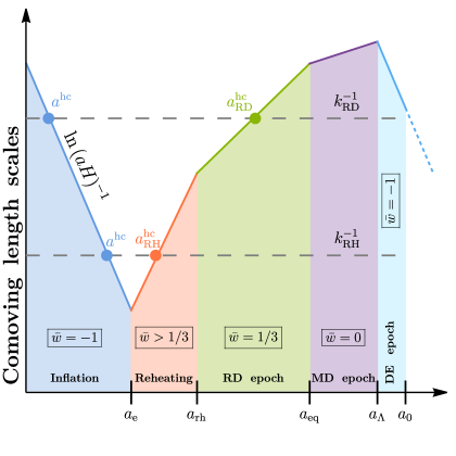
Figure 1: Evolution of cosmological comoving length scales with the scale factor at different epochs of the evolution of the universe. Here “RD” stands for radiation domination, “MD” implies matter domination, and “DE” indicates dark energy domination. In each case corresponding equation of state is also mentioned.

We adopt the following Ahmed:2021fvt parametrization of the inflaton width $\Gamma_{\phi}$:

$$\Gamma_{\phi}=\Gamma_{\phi}^{e}\left(\frac{a_{e}}{a}\right)^{\beta}\,,$$ (7)

where $a_{e}$ is the initial value of the scale factor, indicating the end of inflation, $\Gamma_{\phi}^{e}$ denotes the inflaton width at $a=a_{e}$, while $\beta$ is assumed to be a constant parameter. The above parametrization of the inflaton width can be systematically derived for a homogeneous inflaton condensate with a power-law evolution of the inflaton energy density, assuming massless final states, as elaborated in Appendix. A adopting the $\alpha$-attractor T-model of inflation. More generically, such a parametrization is valid for osciallation of the inflaton in any monomial potential during reheating. In addition, as shown in Garcia:2020wiy ; Ahmed:2022tfm , the generic power-law form of the inflaton width is also well justified if the time dependence of $\Gamma_{\phi}$ arises due to kinematical suppression effects for non-zero final state masses. Further, a general time (temperature) dependent dissipation rate can have several physical origins as discussed in Sec.3 of Ref. Co:2020xaf . It is worth to realize and emphasize that corrections that originate from kinematical mass effects do not change the form of $a$-dependence of the inflaton width, it turns out they merely modify the power $\beta$ in (7). In the following part, we will show how $\beta$ can be connected to the underlying inflationary potential.

The Hubble rate, $H$, evolves according to the Friedmann equation

$$H^{2}=\frac{\rho_{\rm{tot}}}{3M_{P}^{2}}\, \rho_{\rm{tot}}=\rho_{\phi}+\rho_{\text{\tiny SM}}\,.$$ (8)

The initial conditions for the inflaton and SM radiation are given by

$$\rho_{\phi}(a_{e})\equiv\rho_{e}\,, \rho_{\text{\tiny SM}}(a_{e})=0\,.$$ (9)

At early times, the term associated with the expansion, i.e., $3\,(1+\bar{w})\,H\rho_{\phi},$ typically dominates over the interaction term $(1+\bar{w})\,\Gamma_{\phi}\,\rho_{\phi}$. The right-hand side of the first Boltzmann equation (2.1) can then be neglected, and straightforward integration gives a solution for the inflaton energy density during the oscillatory phase

$$\rho_{\phi}^{\text{\tiny{RH}}}(a)\simeq\rho_{e}\left(\frac{a_{e}}{a}\right)^{\frac{6\,n}{n+1}},\leavevmode\nobreak\ \text{for}\leavevmode\nobreak\ a\in[a_{e},a_{\text{rh}})\,,$$ (10)

where the value of the inflaton energy density at the end of inflation can be expressed in terms of the initial value of the Hubble rate, $H_{e}$, though the Friedmann equation, i.e., $\rho_{e}=3\,M_{P}^{2}\,H_{e}^{2}$. During the early stages of reheating, one can neglect the radiation contribution to the total energy density, i.e., $\rho_{\rm{tot}}(a_{e})\simeq\rho_{e}$, which allows us to find the evolution of the Hubble rate

$$H^{\text{\tiny{RH}}}(a)\simeq H_{e}\left(\frac{a_{e}}{a}\right)^{\frac{3\,n}{n+1}}\,,\leavevmode\nobreak\ \text{for}\leavevmode\nobreak\ a\in[a_{e},a_{\text{rh}})\,.$$ (11)

Substituting Eq. (10) and (11) into the second Boltzmann equation in Eq. (2.1), leads to

$$\rho_{\text{\tiny SM}}^{\text{\tiny{RH}}}(a) \simeq\left(\frac{6\,n}{n+1}\right)\cdot\Gamma_{\phi}^{e}\,H_{e}\,M_{P}^{2}\begin{cases}\frac{n+1}{n+4-\beta\,(n+1)}\bigg{[}\left(\frac{a_{e}}{a}\right)^{\beta+\frac{3\,n}{n+1}}-\left(\frac{a_{e}}{a}\right)^{4}\bigg{]},&\beta\neq\frac{n+4}{n+1},\\ \left(\frac{a_{e}}{a}\right)^{4}\ln{\left(\frac{a}{a_{e}}\right)},&\beta=\frac{n+4}{n+1},\end{cases}\,,\leavevmode\nobreak\ a_{e}<a\leq a_{\text{rh}}.$$ (12)

which can further be written as

$$\rho_{\text{\tiny SM}}^{\text{\tiny{RH}}}(a) \approx\rho_{\text{rh}}\,\left(\frac{a_{\text{rh}}}{a}\right)^{4}\,\begin{cases}\left[\frac{1-\left(a_{e}/a\right)^{\frac{\beta\,(n+1)-(n+4)}{n+1}}}{1-\left(a_{e}/a_{\text{rh}}\right)^{\frac{\beta\,(n+1)-(n+4)}{n+1}}}\right],&\beta\neq\frac{n+4}{n+1},\\ \frac{\ln{(a/a_{e})}}{\ln{(a_{\text{rh}}/a_{e})}},&\beta=\frac{n+4}{n+1},\end{cases}\,,\leavevmode\nobreak\ a_{e}<a\leq a_{\text{rh}},$$ (13)

where we have used the value of the radiation energy density at the end of reheating, defined by the inflaton-radiation equality

$$\rho_{\phi}^{\text{\tiny{RH}}}(a_{\text{rh}})=\rho_{\text{\tiny SM}}^{\text{\tiny{RH}}}(a_{\text{rh}})\equiv\rho_{\text{rh}}.$$ (14)

There is a comment here regarding continuity of $\rho_{\text{\tiny SM}}^{\text{\tiny{RH}}}(a)$ as a function of $n$ at $\beta=(n+4)/(n+1)$. Within any given inflaton model, $\beta$ is a fixed function of $n$, e.g., in the case of the inflaton Yukawa interactions $\beta=\beta_{\psi}=3(n-1)/(n+1)$. Then, $\rho_{\text{\tiny SM}}^{\text{\tiny{RH}}}(a)$ should be a continuous function of $n$, including the values of $n$ that follows from the condition $\beta=(n+4)/(n+1)$. Indeed $\rho_{\text{\tiny SM}}^{\text{\tiny{RH}}}(a)$ given by Eq. (12), does satisfy this condition. To prove the continuity, it is essential to keep both terms in the bracket of Eq. (12). However, to perform further analytical calculations, we will be dropping one of those terms at a time. Therefore cases $\beta\ll(n+4)/(n+1)$ and $\beta\gg(n+4)/(n+1)$ will appear, and it is important to note that such approximations are not applicable in the close vicinity of $\beta=(n+4)/(n+1)$.

As the inflaton energy density dominates the early stages of reheating, the background dynamics is determined by the value of $\bar{w}$, whereas the behavior of the SM sector depends on both $\bar{w}$ and $\beta$. Note that, for $\beta<(n+4)/(n+1)$, the first term in the square bracket in (12) dominates, whereas if $\beta>(n+4)/(n+1)$ the energy density of the radiation bath decreases as $a^{-4}$. Thus, depending on the value of $\beta+3\,n/(n+1)$, one obtains a very different evolution of the radiation sector, which implies a non-trivial scaling of a thermal bath temperature $T$ with the scale factor during reheating. In particular, the temperature of the SM sector is measured by the radiation energy density

$$T(a)=\left(\frac{30}{\pi^{2}g_{\star\rho}(T)}\right)^{1/4}\rho_{\text{\tiny SM}}^{1/4}(a)\,,$$ (15)

where $g_{\star}(T)$ counts the effective number of relativistic degrees of freedom at temperature $T$. Utilizing (12), one finds that during the non-standard phase of reheating, $T$ behaves for $a_{e}<a\leq a_{\text{rh}}$ as

$$T^{\text{\tiny{RH}}}(a)\approx\left[\frac{180\,n\;\Gamma_{\phi}^{e}H_{e}M_{P}^{2}}{(n+1)\,\pi^{2}g_{\star\rho}(T)}\right]^{1/4}\begin{cases}\frac{n+1}{n+4-\beta\,(n+1)}\,\bigg{[}\left(\frac{a_{e}}{a}\right)^{\beta+\frac{3\,n}{n+1}}-\left(\frac{a_{e}}{a}\right)^{4}\bigg{]}^{1/4},&\beta\neq\frac{n+4}{n+1},\\ \frac{a_{e}}{a}[\ln{(a/a_{e})}]^{1/4},&\beta=\frac{n+4}{n+1}\end{cases}\,.$$ (16)

The scale factor at the end of reheating can be determined from Eqs. (10) and (12) as follows

$$a_{\text{rh}}=a_{e}\begin{cases}\left(\frac{n+4-\beta\,(n+1)}{2\,n}\,\frac{H_{e}}{\Gamma_{\phi}^{e}}\right)^{\frac{n+1}{n\,(3-\beta)-\beta}},&\beta\ll\frac{n+4}{n+1},\\ \left(\frac{H_{e}}{\Gamma_{\phi}^{e}}\,\frac{n-2}{n}\right)^{\frac{n+1}{2\,(n-2)}}\mathcal{W}^{\frac{n+1}{2\,(2-n)}}\,\left(\frac{H_{e}}{\Gamma_{\phi}^{e}}\frac{n-2}{n}\right),&\beta=\frac{n+4}{n+1},\\ \left(\frac{\beta-4+n\,(\beta-1)}{2\,n}\frac{H_{e}}{\Gamma_{\phi}^{e}}\right)^{\frac{n+1}{2\,(n-2)}},&\beta\gg\frac{n+4}{n+1}\,,\end{cases}$$ (17)

where $\mathcal{W}[z]$ denotes the Lambert $\mathcal{W}$-function. Note that in order to obtain the above result, we had to drop either the first or the second term in the bracket in Eq. (12).

During non-instantaneous decay of the inflaton, the bath temperature can rise to several orders of magnitude above the reheating temperature Giudice:2000ex . This happens at $a=a_{\rm{max}}$, defined via

$$a_{\rm{max}} \equiv a_{e}\begin{cases}\left[\frac{1}{4}\left(\beta+\frac{3\,n}{n+1}\right)\right]^{\frac{n+1}{\beta\,(n+1)-(n+4)}},&\beta\neq\frac{n+4}{n+1}\,,\\ \exp(1/4),&\beta=\frac{n+4}{n+1}\,,\end{cases}$$ (18)

so that the maximum temperature of the radiation bath is

$$T_{\tiny{\rm{max}}}\equiv\,T^{\text{\tiny{RH}}}(a_{\rm{max}}) \approx\left(\frac{180\,n\,M_{P}^{2}}{(n+1)\,\pi^{2}\,g_{\star\rho}(T)}\,\Gamma_{\phi}^{e}\,H_{e}\right)^{1/4}$$

$$\times\begin{cases}\left[\frac{n+1}{n+4-\beta\,(n+1)}\right]^{1/4}\,\bigg{[}\frac{1}{4}\left(\beta+\frac{3\,n}{n+1}\right)\bigg{]}^{\frac{\beta+n\,(\beta+3)}{4\,\left((n+4)-\beta\,(n+1)\right)}},&\beta\ll\frac{n+4}{n+1},\\ \frac{1}{\sqrt{2}}e^{-1/4},&\beta=\frac{n+4}{n+1},\\ \left[\frac{n+1}{\beta-4+n\,(\beta-1)}\right]^{1/4}\,\bigg{[}\frac{1}{4}\,\left(\beta+\frac{3\,n}{n+1}\right)\bigg{]}^{\frac{n+1}{n+4-\beta\,(n+1)}},&\beta\gg\frac{n+4}{n+1}\,.\end{cases}$$ (19)

From the discussion so far, it is understandable that once one specifies the inflaton potential $V(\phi)$ and the form of the inflaton-SM interactions (the “model”), $\bar{w},H_{e},\beta,\Gamma_{\phi}^{e}$ can be determined.

Before proceeding further, let us briefly discuss the details of inflaton dynamics during the oscillatory phase. In the FLRW background, the classical equation of motion (EoM) for the inflaton is given by

$$\ddot{\phi}+3\,H\,\dot{\phi}+\frac{\partial V(\phi)}{\partial\phi}=0\,,$$ (20)

where we have assumed that $\phi$ is spatially homogeneous. During the period of reheating, the oscillating inflaton field with a time-dependent amplitude can be parametrized as Ichikawa:2008ne ; Kainulainen:2016vzv ; Clery:2021bwz ; Co:2022bgh ; Garcia:2020wiy ; Ahmed:2022qeh .

$$\phi(t)=\varphi(t)\,.\,\mathcal{P}(t)\,.$$ (21)

Here, $\mathcal{P}(t)$ is a quasi-periodic, fast-oscillating function, and $\varphi(t)$ is a slowly-varying envelope. It is instructive to introduced the effective mass of the inflaton

$$m_{\phi}^{2}\equiv\frac{\partial^{2}V(\phi)}{\partial\phi^{2}}\Bigg{|}_{\phi=\varphi}=\frac{n\,\left(2n-1\right)}{3\,\alpha}\,\frac{\Lambda^{4}}{M_{P}^{2}}\,\left(\frac{\rho_{\phi}}{\Lambda^{4}}\right)^{\frac{n-1}{n}}\,.$$ (22)

The slow-roll evolution of the inflaton field during cosmic inflation can be parameterized by the so-called potential slow-roll parameters

$$\epsilon_{V}=\frac{M_{P}^{2}}{2}\,\left(\frac{V^{\prime}(\phi)}{V(\phi)}\right)^{2}, \eta_{V}=M_{P}^{2}\,\frac{V^{\prime\prime}(\phi)}{V(\phi)}\,,$$ (23)

that are related to the cosmological observables, namely the spectral index $n_{s}$ and the tensor-to-scalar ratio $r$ via

$$r\simeq 16\,\epsilon_{V}\,, n_{s}\simeq 1-6\,\epsilon_{V}+2\eta_{V}\,.$$ (24)

At the very end of inflation, $\ddot{a}=0$, and the first potential slow-roll parameter is $\epsilon_{V}\simeq 1$. This condition determines the field at $a=a_{e}$, i.e.,

$$\varphi_{e}=\sqrt{\frac{3}{2}}\,M_{P}\,\sinh^{-1}\left[\frac{2\,n}{\sqrt{3\,\alpha}}\right]\,.$$ (25)

Moreover, at $a=a_{e}$, the potential energy of $\phi$ matches with its kinetic energy, so that

$$\rho_{e}=\frac{3}{2}\,V(\varphi_{e})\,,$$ (26)

where we have assumed that $\mathcal{P}(a_{e})=1$. From the above expression, we see that $\rho_{e}$ has a very mild dependence on the index $n$ for a fixed $\alpha$ and $\Lambda$. For example, with $\alpha=1/6$ and $\Lambda=3\times 10^{-3}\,M_{P}$, we find $\rho_{e}\simeq 2\times 10^{63}\,\text{GeV}^{4}$ for $n\in[2\,,10]$.

2.2 Models of inflaton-matter interactions

Let us now specify interactions between the inflaton and other matter particles. Here, we assume that perturbative expansion is justified while calculating the quantum production of radiation (reheating) from the vacuum in the classical inflaton background. Once the inflaton couples to matter fields, its oscillations are severely damped by the decay. Without going into the details of the UV completion, we consider four possible interaction vertices

$$\mathcal{L}_{\text{int}}\supset\mathcal{L}_{SS\phi}+\mathcal{L}_{\psi\psi\phi}+\mathcal{L}_{VV\phi}+\mathcal{L}_{aa\phi}\,,$$ (27)

and parametrize them as

$$\mathcal{L}_{SS\phi}\supset g_{S\phi}\,SS\,\phi\,,$$

$$\mathcal{L}_{\psi\psi\phi}\supset g_{\psi\phi}\,\overline{\psi}\,\psi\,\phi\,,$$

$$\mathcal{L}_{VV\phi}\supset g_{V\phi}\,V_{\mu}\,V^{\mu}\,\phi\,,$$

$$\mathcal{L}_{aa\phi}\supset h_{a\phi}\,\partial_{\mu}a\,\partial^{\mu}a\,\phi\,,$$ (28)

where $S\,,V\,,\psi,a$ are generic scalar field, vector boson, Dirac fermion, and particles with derivative interactions (e.g., axion-like particles), respectively. We refer to scenarios with an inflaton-matter coupling specified as to models and consider them individually. It is important to stress that in the adopted parametrization, the coupling $g_{S\phi}$ and $g_{V\phi}$ have dimensions of mass, $g_{\psi\phi}$ is dimensionless, while $h_{a\phi}$ has inverse mass dimension. Let us also notice that once the model of reheating is specified, $\Gamma_{\phi}^{e}$ can be calculated, see Eq. (107), in terms of the model coupling $g_{i\phi}$ ($i\in SS\,,\psi\psi\,,\mathcal{VV}\,,aa$) and parameters of the inflaton potential, which also determines the value of the $\beta$ parameter. Moreover, the time-averaged EoS parameter $\bar{w}$ is predicted solely by the shape of the inflaton potential Eq. (4). Within a given model of inflaton-matter interaction, we adopt the following set of independent parameters 

$$\{\Gamma_{\phi\to f}^{e}\,,\Lambda,\,n\}\,,$$ (29)

where $f=SS,\,\psi\psi,\,\mathcal{VV}\,,aa$.

3 Spectrum of Primordial Gravitational Waves

Here we briefly summarize formalism to calculate the spectrum of a stochastic GW background of primordial origin. The complete derivations can be found in, for example, Refs. Boyle:2005se ; Watanabe:2006qe ; Saikawa:2018rcs ; Caprini:2018mtu , hence without going into the details, here we highlight the salient points that help in obtaining the final expression for primordial GW spectrum. We shall mainly stick to the convention followed in Ref. Saikawa:2018rcs while elaborating on the definition of different relevant quantities.

GWs are described as the tensor metric perturbations in a spatially-flat FLRW Universe

$$ds^{2}=dt^{2}-a^{2}(t)\,\left(\delta_{ij}+h_{ij}(t,{\bf x})\right)\,dx^{i}\,dx^{j}\,.$$ (30)

Tensor fluctuations are assumed to be small perturbations, i.e., $|h_{ij}|\ll 1$, satisfying the transverse-traceless conditions, $h_{i}^{i}=\partial^{i}\,h_{ij}=0$. The GWs equation of motion follows the Einstein equations linearized to first order in $h_{ij}$ over the FRLW background

$$\ddot{h}_{ij}+3\,H\,\dot{h}_{ij}-\frac{\nabla^{2}}{a^{2}}\,h_{ij}=16\,\pi\,G\,\Pi_{ij}^{\text{TT}}\,,$$ (31)

with $\Pi_{ij}^{\text{TT}}$ being the transverse and traceless part of the anisotropic stress tensor. It is instructive to decompose the perturbation $h_{ij}$ over two polarization states $\lambda$ as

$$h_{ij}(t\,,{\bf x})=\sum_{\lambda=+\,,\times}\int\,\frac{d^{3}{\bf k}}{(2\,\pi)^{3}}\,h^{\lambda}(t\,,{\bf k})\,\epsilon_{ij}^{\lambda}({\bf k})\,\exp\left(i\,{\bf k}\cdot{\bf x}\right)\,,$$ (32)

where $\epsilon_{ij}^{\lambda}({\bf k})$ are spin-2 polarization tensors satisfying orthonormality and completeness relations

$$\sum_{ij}\epsilon_{ij}^{\lambda}\,\left(\epsilon_{ij}^{\lambda^{\prime}}\right)^{\star}=2\,\delta^{\lambda\lambda^{\prime}}\,,$$

$$\sum_{\lambda=+\,,\times}\,\epsilon_{ij}^{\lambda}({\bf\hat{k}})\,\epsilon_{lm}^{\lambda}\,({\bf\hat{k}})=P_{il}\,P_{jm}+P_{im}\,P_{jl}-P_{ij}\,P_{lm}\,,$$ (33)

with $P_{ij}=\delta_{ij}-\hat{k}_{i}\,\hat{k}_{j}$ being the projection operator and $\bf\hat{k}$ being the unit vector along the direction of $\bf k$.

The mode function $h^{\lambda}(t,\bf{k})\equiv h_{\bf k}^{\lambda}$ satisfies the following equation:

$$\ddot{h}_{\bf k}^{\lambda}+3\,H\,\dot{h}_{\bf k}^{\lambda}+\frac{k^{2}}{a^{2}}\,h_{\bf k}^{\lambda}=16\,\pi\,G\,\Pi_{\bf k}^{\lambda}\,,$$ (34)

where $\Pi_{\bf k}^{\lambda}$ is the Fourier components of $\Pi_{ij}^{\text{TT}}$. It is convenient rewrite the above equation in conformal coordinates

$$\left(h_{\bf k}^{\lambda}\right)^{\prime\prime}+2\,\frac{a^{\prime}}{a}\left(h_{\bf k}^{\lambda}\right)^{\prime}+k^{2}\,h_{\bf k}^{\lambda}=16\,\pi\,G\,a^{2}\,\Pi_{\bf k}^{\lambda}\,,$$ (35)

where prime denotes a derivative with respect to the conformal time coordinate, defined by $dt=ad\tau$. Eq. (35) admits approximate analytical solutions in two extreme regimes as follows

• Super-Hubble scale:
  For modes far outside the Hubble horizon, i.e., $k\ll aH$, one can write Eq. (35) as

  $$\left(h_{\bf k}^{\lambda}\right)^{\prime\prime}+2\,\frac{a^{\prime}}{a}\left(h_{\bf k}^{\lambda}\right)^{\prime}\approx 0\,\implies a^{-2}\,\left(a^{2}\,h_{\bf k}^{\lambda\prime}\right)^{\prime}\approx 0\,,$$ (36)

  where we have ignored the source term. This equation has a solution of the form

  $$h_{\bf k}^{\lambda}(\tau)=\mathcal{C}_{1}+\mathcal{C}_{2}\int\,\frac{d\tau^{\prime}}{a(\tau^{\prime})^{2}}\,,$$ (37)

  where $\mathcal{C}_{1,2}$ are constants of integration. The second term in the above expression decays with time. Therefore, ignoring the decaying term, one concludes that $h_{\bf k}^{\lambda}$ stays constant for super-Hubble modes Watanabe:2006qe ; Saikawa:2018rcs . At some point after inflation, these modes become sub-Hubble, i.e., $k>a\,H$ and re-enter the horizon.

• Sub-Hubble scale:
  After the end of inflation, modes eventually re-enter the horizon $(k>a\,H)$ and start to oscillate. In this case, Eq. (35) can be solved by assuming a solution of the form

  $$h_{\bf k}^{\lambda}=A(\tau)\,\exp\left(i\,B(\tau)\right)\,,$$ (38)

  where $A$ and $B$ are real functions. Substituting this in Eq. (34), and comparing the real and imaginary components, we obtain

  $$A^{\prime\prime}-A\,\left(B^{\prime}\right)^{2}+\frac{2\,a^{\prime}}{a}\,A^{\prime}+k^{2}\,A=0\,,$$

  $$2\,A^{\prime}\,B^{\prime}+A\,B^{\prime\prime}+\frac{2\,a^{\prime}}{a}\,A\,B^{\prime}=0\,,$$ (39)

  where again, we have dropped the source term. Now, considering the oscillation to be very rapid compared to the time variation of the amplitude, and the modes to be well inside the horizon $k\gg a^{\prime}/a$, we obtain from the first equation

  $$B(\tau)=\pm k\,\tau+\text{constant}\,,$$ (40)

  which on substitution in the second equation brings us to

  $$A(\tau)\propto a(\tau)^{-1}\,.$$ (41)

  The behaviour of the mode function $h_{\bf k}^{\lambda}$ is thus described by a WKB solution of the from

  $$h_{\bf k}^{\lambda}\simeq\left(C/a\right)\,\exp\left(\pm ik\,\tau\right),$$ (42)

  where $C$ is some arbitrary constant.

The energy density carried by the GWs is given Maggiore:1999vm ; Watanabe:2006qe ; Saikawa:2018rcs ; Caprini:2018mtu by

$$\rho_{\text{GW}}=\frac{1}{64\pi Ga^{2}}\left\langle\left(\partial_{\tau}h_{ij}\right)^{2}+\left(\nabla h_{ij}\right)^{2}\right\rangle\,,$$ (43)

where $\langle...\rangle$ denotes the spatial average. As it could be seen from Eq. (34), once a particular mode re-enters (in other words crosses) the horizon, i.e., $k>aH$, the corresponding mode function obeys $|\partial h_{\bf k}^{\lambda}(\tau)/\partial\tau|^{2}=k^{2}\,|h_{\bf k}^{\lambda}(\tau)|^{2}$, therefore the energy density could be written as

$$\rho_{\text{GW}}=\frac{1}{32\,\pi\,G}\,\int d\,\ln k\,\left(\frac{k}{a}\,\right)^{2}\,\left[\frac{k^{3}}{\pi^{2}}\sum_{\lambda}\left|h_{\bf k}^{\lambda}\right|^{2}\right].$$ (44)

It is useful to define the spectral GW density per logarithmic wavenumber interval, normalized to the critical density $\rho_{c}=3\,H^{2}/(8\,\pi\,G)$ as follows

$$\Omega_{\text{GW}}(\tau,k)=\frac{1}{\rho_{c}}\,\frac{d\rho_{\text{GW}}}{d\log k}\,.$$ (45)

Then, starting with Eq. (43), one can obtain Watanabe:2006qe ; Saikawa:2018rcs

$$\Omega_{\text{GW}}(\tau\,,k)=\frac{1}{12}\,\left(\frac{k}{a(\tau)\,H(\tau)}\right)^{2}\mathcal{P}_{T,\text{prim}}\,\mathcal{T}(\tau,k)\,,$$ (46)

where the primordial power spectrum has been defined as

$$\mathcal{P}_{T,\text{prim}}\equiv\frac{k^{3}}{\pi^{2}}\,\sum_{\lambda}\left|h_{{\bf k}\,,\text{prim}}^{\lambda}\right|^{2}\,,$$ (47)

with the primordial mode function $h_{{\bf k}\,,\text{prim}}^{\lambda}$ defined as the mode function $h_{{\bf k}}^{\lambda}(\tau)$ at some moment shortly after the end of inflation, when all the modes have already exited the horizon.

The primordial tensor power spectrum $\mathcal{P}_{T,\text{prim}}$ is determined by the Hubble parameter at the time when the corresponding mode crosses the horizon during inflation $(k=aH)$ Watanabe:2006qe ; Saikawa:2018rcs ; Caprini:2018mtu

$$\mathcal{P}_{T,\text{prim}}=\frac{2\,H^{2}}{\pi^{2}\,M_{P}^{2}}\Bigg{|}_{k=a\,H}\,,$$ (48)

where we have used the mode solutions by matching the sub-Hubble modes (during inflation) with the super-Hubble modes (at the end of inflation) at $k=a\,H$ Boyle:2005se ; Caprini:2018mtu . The transfer function, $\mathcal{T}(\tau\,,k)$, adopted in Eq.(46), connects primordial mode functions with mode functions at some later time $h_{\bf k}^{\lambda}(\tau)$ as Boyle:2005se ; Saikawa:2018rcs

$$\mathcal{T}(\tau\,,k)=\left|\frac{h_{\bf k}^{\lambda}(\tau)}{h_{{\bf k},\text{prim}}^{\lambda}}\right|^{2}\,.$$ (49)

As shown earlier, the modes $h_{{\bf k}}^{\lambda}$ remain constant on super-horizon scales, while they decrease as $a^{-1}$ once they re-enter the Hubble horizon. In other words, in the sub-horizon regime, i.e., $k>aH$, $h_{{\bf k}}^{\lambda}=\left(a^{\text{hc}}/a\right)\,h_{{\bf k}}^{\text{hc},\lambda}$; therefore, the transfer function could be written Kuroyanagi:2008ye ; Opferkuch:2019zbd ; Allahverdi:2020bys as

$$\mathcal{T}(\tau\,,k)=\frac{1}{2}\,\left(\frac{a^{\text{hc}}}{a}\right)^{2}\,,$$ (50)

where the prefactor 1/2 appears due to oscillation-averaging the tensor mode functions Saikawa:2018rcs ; Choi:2021lcn ; Figueroa:2018twl and $a^{\text{hc}}$ is scale factor at the horizon crossing. As evident from Eq. (50), the transfer function characterizes the expansion history between the moment of horizon crossing $\tau=\tau^{\text{hc}}$ of a given mode $k$ and some later moment $\tau>\tau^{\text{hc}}$. From Eq. (46), one can see that the spectral GW energy density at the present time is given by

$$\Omega_{\text{GW}}^{(0)}(k)=\frac{1}{24}\left(\frac{k}{a_{0}H_{0}}\right)^{2}\mathcal{P}_{T,\text{prim}}\left(\frac{a^{\text{hc}}}{a_{0}}\right)^{2}\,,$$ (51)

where $a_{0}=1$ and $H_{0}$ are respectively the scale factor and the Hubble parameter measured today.

One anticipates that $\Omega_{\text{GW}}^{(0)}(k)$ has a power-law dependence on $k$. Using the fact that $k=a^{\text{hc}}H(a^{\text{hc}})$, and the equation-of-state parameter after the horizon crossing is $\bar{w}$, one obtains

$$a^{\text{hc}}\propto k^{\frac{n+1}{1-2\,n}}\,$$ (52)

Hence, from Eq. (51) we find the following scaling applies

$$\Omega_{\text{GW}}^{(0)}(k)\propto k^{\frac{2\,n-4}{2\,n-1}}\,.$$ (53)

Let us now find the coefficient of proportionality in Eq. (53). This coefficient might, in particular, depend on parameters such as, e.g., the inflaton width $\Gamma_{\phi}^{e}$ at the end of inflation, which, in turn, is determined by the inflaton-matter couplings. The sensitivity of the spectral GW energy density upon the inflaton couplings is one of the central tasks of this study. We will determine the present value of the spectral GW energy density for the modes re-entering the horizon at different epochs; after the end of reheating, during RD, and prior to the onset of RD, that is, during inflaton domination (reheating). At first, let us assume that the horizon re-entry happens during the RD epoch after the end of reheating, i.e., $a^{\text{hc}}_{\text{RD}}\in(a_{\rm rh},a_{\rm eq})$. In this case, we reproduce the standard scale-invariant result for the spectral GW energy density

$$\Omega_{\text{GW}}^{(0),\rm{RD}}=\frac{\mathcal{P}_{T,\text{prim}}}{24}\,\left(\frac{a^{\text{hc}}_{\text{RD}}\,H^{\text{hc}}_{\text{RD}}}{a_{0}\,H_{0}}\right)^{2}\,\left(\frac{a^{\text{hc}}_{\text{RD}}}{a_{0}}\right)^{2}=\Omega_{\gamma}^{(0)}\,\frac{\mathcal{P}_{T,\text{prim}}}{24}\,\mathcal{F}(g_{\star})\,,$$ (54)

where the function $\mathcal{F}(g_{\star})\equiv\frac{g_{\star\rho}^{\text{RH}}}{g_{\star\rho}^{0}}\,\left(\frac{g_{\star s}^{0}}{g_{\star s}^{\text{RH}}}\right)^{\frac{4}{3}}$ tracks the number of degrees of freedom from the end of reheating till present, and $\Omega_{\gamma}^{(0)}=\rho_{\gamma,0}/\rho_{c}=2.47\times 10^{-5}\,h^{-2}$ is the fraction of the energy density of photons at the present epoch. Here we have assumed entropy conservation from the moment of horizon crossing (RD) till today, implying $T\propto a^{-1}\,g_{\star s}^{-1/3}$. On the other hand, if the horizon crossing happens during reheating, before the radiation era, i.e., $a^{\text{hc}}_{\text{RH}}\in(a_{e},a_{\rm rh})$, one obtains

$$\Omega_{\text{GW}}^{(0),\rm{RH}}=\frac{\mathcal{P}_{T,\text{prim}}}{24}\,\left(\frac{H^{\text{hc}}_{\text{RH}}}{H_{0}}\right)^{2}\,\left(\frac{a^{\text{hc}}_{\text{RH}}}{a_{0}}\right)^{4}=\Omega_{\text{GW}}^{(0),\text{RD}}\,\left[\left(\frac{g_{\star\rho}^{\text{rh}}}{g_{\star\rho,\text{RD}}^{\text{hc}}}\right)^{\frac{3}{4}}\,\frac{g_{\star s,\text{RD}}^{\text{hc}}}{g_{\star s}^{\text{rh}}}\right]^{\frac{4}{3}}\,\left(\frac{a^{\text{hc}}_{\text{RH}}}{a_{\text{rh}}}\right)^{\frac{4-2\,n}{n+1}}\,,$$ (55)

where we have used the following relations:

$$\left(\frac{a_{\text{rh}}}{a^{\text{hc}}_{\text{RD}}}\right)^{4}\left(\frac{H_{\text{rh}}}{H^{\text{hc}}_{\text{RD}}}\right)^{2}=\frac{g_{\star\rho}^{\text{rh}}}{g_{\star\rho,\text{RD}}^{\text{hc}}}\,\left(\frac{g_{\star s,\text{RD}}^{\text{hc}}}{g_{\star s}^{\text{rh}}}\right)^{4/3}\,,$$

$$\left(\frac{a^{\text{hc}}_{\text{RH}}}{a_{\text{rh}}}\right)^{4}\left(\frac{H^{\text{hc}}_{\text{RH}}}{H_{\text{rh}}}\right)^{2}=\left(\frac{a^{\text{hc}}_{\text{RH}}}{a_{\text{rh}}}\right)^{\frac{4-2\,n}{n+1}}\,.$$ (56)

Now, for the re-entry of the modes happening during the period of reheating, redshifting the GW frequency $f$ to present, we obtain Saikawa:2018rcs

$$f=\frac{k}{2\pi}\frac{1}{a_{0}}=\frac{H^{\text{hc}}_{\text{RH}}}{2\,\pi}\,\frac{a^{\text{hc}}_{\text{RH}}}{a_{0}}=\frac{\rho_{\text{rh}}^{1/2}}{2\,\pi\,\sqrt{3\,M_{P}^{2}}}\,\frac{a^{\text{hc}}_{\text{RH}}}{a_{0}}\,\left(\frac{a_{\text{rh}}}{a^{\text{hc}}_{\text{RH}}}\right)^{\frac{3\,n}{n+1}}\,,$$ (57)

where $\rho_{\text{rh}}$ in the total energy density of the Universe at the end of reheating.

There exists an upper bound on frequencies, dictated by the modes that re-entered the horizon after the end of inflation

$$f_{\text{max}}=\frac{H_{e}}{2\pi}\,\frac{a_{e}}{a_{0}}\simeq\frac{\Lambda^{2}\,(n\,\sqrt{2})^{n}}{2\,\sqrt{2}\pi\,M_{P}}\,\left(\frac{g_{\star s}(T_{0})^{\frac{1}{3}}\,T_{0}}{g_{\star s}(T_{\text{rh}})^{\frac{1}{3}}\,T_{\text{rh}}}\right)$$

$$\times\begin{cases}\left[\left(n\sqrt{2}\right)^{n}\,\left(\frac{(n+4)-\beta\,(n+1)}{2\,n}\right)\,\frac{\Lambda^{2}}{\sqrt{2}\,M_{P}\,\Gamma_{\phi}^{e}}\right]^{\frac{n+1}{n\,(\beta-3)+\beta}},&\beta\ll\frac{n+4}{n+1}\,,\\ \left[\left(n\sqrt{2}\right)^{n}\,\frac{\Lambda^{2}}{\sqrt{2}\,M_{P}\,\Gamma_{\phi}^{e}}\,\frac{n-2}{n}\right]^{\frac{n+1}{2\,(2-n)}}\mathcal{W}^{\frac{n+1}{2\,(2-n)}}\left[\left(n\sqrt{2}\right)^{n}\,\frac{\Lambda^{2}}{\sqrt{2}\,M_{P}\,\Gamma_{\phi}^{e}}\,\frac{n-2}{n}\right],&\beta=\frac{n+4}{n+1}\,,\\ \left[\left(n\sqrt{2}\right)^{n}\left(\frac{\beta-4+n\,(\beta-1)}{2\,n}\right)\,\frac{\Lambda^{2}}{\sqrt{2}\,M_{P}\,\Gamma_{\phi}^{e}}\right]^{\frac{1+n}{4-2\,n}},&\beta\gg\frac{n+4}{n+1}\,,\end{cases}$$ (58)

while modes with frequencies $f>f_{\text{max}}$ are never produced. It is worth mentioning here that we are working in the small-field limit, where $\phi_{e}\simeq\sqrt{2}\,n\,M_{P}$ and $H_{e}=\sqrt{\rho_{e}/\left(3\,M_{P}^{2}\right)}\simeq\Lambda^{2}\,\left(n\,\sqrt{2}\right)^{n}/\left(\sqrt{2}\,M_{P}\right)$. Using Eq. (57) we can relate the ratio of the scale factors and the frequency $f$, arriving at

$$\Omega_{\text{GW}}^{(0),\rm{RH}}=\Omega_{\text{GW}}^{(0),\rm{RD}}\,\widetilde{\mathcal{F}}(g_{\star})\left[\frac{2\pi}{\sqrt{3}}\frac{T_{0}}{M_{P}}\,\left(\frac{30}{\pi^{2}\,g_{\star\rho}^{\text{rh}}}\right)^{-\frac{1}{4}}\right]^{\frac{4-2\,n}{2\,n-1}}\rho_{\text{rh}}^{\frac{2-n}{4\,n-2}}\,f^{\frac{2\,n-4}{2\,n-1}}\,,$$ (59)

with

$$\widetilde{\mathcal{F}}(g_{\star})\equiv\left(\frac{g_{\star s}^{0}}{g_{\star s}^{\text{rh}}}\right)^{\frac{4-2\,n}{6\,n-3}}\frac{g_{\star\rho}^{\text{rh}}}{g_{\star\rho,\text{RD}}^{\text{hc}}}\left(\frac{g_{\star s,\text{RD}}^{\text{hc}}}{g_{\star s}^{\text{rh}}}\right)^{4/3}\,,$$ (60)

which shows the blue-tilted behaviour of the spectrum for $\bar{w}>1/3$, which is equivalent to $n>2$. One can then, exploiting Eq. (12) and Eq. (17), rewrite $\rho_{\text{rh}}$ in Eq. (59) in terms of $\Gamma_{\phi}^{e}$ and remaining parameters ($\Lambda,\beta,n$), so that the spectral GW energy density as a function of the frequency measured today reads

$$\Omega_{\text{GW}}^{(0),\text{RH}}(f)\simeq\Omega_{\text{GW}}^{(0),\rm{RD}}\,\widetilde{\mathcal{F}}(g_{\star})\left[\frac{2\pi}{\sqrt{3}}\frac{T_{0}}{M_{P}}\,\left(\frac{30}{\pi^{2}\,g_{\star\rho}^{\text{rh}}}\right)^{-\frac{1}{4}}\right]^{\frac{4-2\,n}{2\,n-1}}\,f^{\frac{2\,n-4}{2\,n-1}}\,\left[\frac{3\,n}{n+1}\,(2\,n^{2})^{n}\,\Lambda^{4}\right]^{\frac{2-n}{4\,n-2}}$$

$$\times\begin{cases}\left(\frac{2\,n}{n+1}\right)^{\frac{n-2}{4\,n-2}}\,\left[\frac{n+4-\beta\,(n+1)}{2\,n}\right]^{\frac{\beta\,(n+1)\,(2-n)}{(2\,n-1)\,(\beta\,(n+1)-3\,n)}}\,\left[\frac{(n\sqrt{2})^{n}\,\Lambda^{2}}{\sqrt{2}\,M_{P}\,\Gamma_{\phi}^{e}}\right]^{\frac{3\,n\,(n-2)}{(1-2\,n)\,(\beta\,(1+n)-3n)}}\,,&\beta\ll\frac{n+4}{n+1}\,,\\[8.0pt] \vartheta^{\frac{n+1}{2n-1}}\mathcal{W}^{\frac{n+1}{1-2\,n}}(\vartheta)\left[\ln{\left(\vartheta^{\frac{n+1}{2n-4}}\mathcal{W}^{\frac{n+1}{4-2\,n}}(\vartheta)\right)}\right]^{\frac{2-n}{4\,n-2}}\,\left[\frac{(n\sqrt{2})^{n}\,\Lambda^{2}}{\sqrt{2}\,M_{P}\,\Gamma_{\phi}^{e}}\right]^{\frac{n-2}{4\,n-2}}\,,&\beta=\frac{n+4}{n+1}\\ \left(\frac{n+1}{2\,n}\right)^{\frac{2-n}{4\,n-2}}\,\left[\frac{\beta\,(n+1)-(n+4)}{2\,n}\right]^{\frac{3\,n}{4\,n-2}}\,\left[\frac{(n\sqrt{2})^{n}\,\Lambda^{2}}{\sqrt{2}\,M_{P}\,\Gamma_{\phi}^{e}}\right]^{\frac{3\,n}{4\,n-2}}\,,&\beta\gg\frac{n+4}{n+1}\,,\end{cases}$$ (61)

with

$$\vartheta\equiv\left[\frac{(n\sqrt{2})^{n}\,\Lambda^{2}}{\sqrt{2}\,M_{P}\,\Gamma_{\phi}^{e}}\right]\,\frac{n-2}{n}\,.$$ (62)

The above expression explicitly shows how the proportionality coefficient of Eq. (53) depends on the inflaton decay width $\Gamma_{\phi}^{e}$ at the end of inflation. Since the only frequency dependence in Eq. (3) enters through $f^{\frac{2\,n-4}{2\,n-1}}$, one can write the full spectrum today in an approximate piecewise form as

$$\Omega_{\text{GW}}^{(0)}(f)\sim\Omega_{\text{GW}}^{(0),\text{RD}}\,\begin{cases}1\,,&f<f_{c}\\[8.0pt] f^{\frac{2\,n-4}{2\,n-1}}\,,&f_{c}<f<f_{\text{max}}\\[8.0pt] 0\,,&f>f_{\text{max}}\end{cases}$$ (63)

where $f_{c}$ can be analytically computed as

$$f_{c}\simeq\left[\frac{n\,(2\,n^{2})^{n}}{n+1}\,\frac{\sqrt{3}\,\pi}{20}\,g_{\star\rho}^{\text{rh}}\,\frac{\Lambda^{4}\,M_{P}}{T_{0}}\,\widetilde{\mathcal{F}}(g_{\star})^{\frac{8\,n-4}{4-2\,n}}\right]^{1/4}$$

$$\times\begin{cases}\left(\frac{2\,n}{n+1}\right)^{\frac{2\,n-1}{4-8\,n}}\,\left[\frac{n+4-\beta\,(n+1)}{2\,n}\right]^{\frac{3\,n}{2\,\left(\beta\,(n+1)-3\,n\right)}}\,\left[\frac{(n\sqrt{2})^{n}\,\Lambda^{2}}{\sqrt{2}\,M_{P}\,\Gamma_{\phi}^{e}}\right]^{\frac{3}{2\,(\beta\,(1+n)-3n)}}\,,&\beta\ll\frac{n+4}{n+1}\,,\\[8.0pt] \vartheta^{\frac{n+1}{4-2\,n}}\mathcal{W}^{\frac{n+1}{2\,n-4}}(\vartheta)\left[\ln{\left(\vartheta^{\frac{n+1}{2n-4}}\mathcal{W}^{\frac{n+1}{4-2\,n}}(\vartheta)\right)}\right]^{1/2}\,\left[\frac{(n\sqrt{2})^{n}\,\Lambda^{2}}{\sqrt{2}\,M_{P}\,\Gamma_{\phi}^{e}}\right]^{-1/4}\,,&\beta=\frac{n+4}{n+1}\\ \left(\frac{n+1}{2\,n}\right)^{\frac{1}{4}}\,\left[\frac{\beta\,(n+1)-(n+4)}{2\,n}\right]^{\frac{3\,n}{8-4\,n}}\,\left[\frac{(n\sqrt{2})^{n}\,\Lambda^{2}}{\sqrt{2}\,M_{P}\,\Gamma_{\phi}^{e}}\right]^{\frac{3\,n}{4\,(1-2\,n)}}\,,&\beta\gg\frac{n+4}{n+1}\,.\end{cases}$$ (64)

Here we would like to emphasize that Eq. (3) is a general expression for GW energy density today, agnostic to the underlying inflaton coupling, and only relies on the fact that the inflaton decay width depends on the scale factor the way it has been assumed in Eq. (7). In Sec. 4 we present plots of $\Omega_{\text{GW}}^{(0)}(f)$ calculated according to Eq. (63) as a function of $f$ for different inflaton models and various choices of parameters $\{g_{i\phi}\,,n\,,\Lambda\}$. It is worth noting the presence of the constant contribution for $f\raise 1.29167pt\hbox{$\;<$\kern-7.5pt\raise-4.73611pt\hbox{$\sim\;$}}f_{c}$.

4 Results and Discussion

So far, we have considered primordial gravitational waves (PGW) and the connection between the spectral energy density of PGW and the inflaton decay width at the end of inflation, $\Gamma_{\phi}^{e}$, i.e., we have found a correspondence between the particle physics model and GW spectrum. Hereafter we assume that all the inflaton decay products belong exclusively to the thermal bath, and they thermalize instantaneously after being produced. In particular, we emphasize that the inflaton does not decay into dark matter (DM) pairs. Below, first, we review existing experimental constraints on the parameter space. Then, we present and discuss results for GWs spectral energy density within each inflaton model defined in Sec. 2.2.

4.1 Constraints on the model parameters

There exist experimental constraints on the parameter space $\{g_{i\phi}\,,\Lambda\,,n\}$ or, equivalently, upon $\{\Gamma_{\phi\to f}^{e}\,,\Lambda,\,n\}$. They will be reviewed shortly below.

4.1.1 $\Delta N_{\text{eff}}$

As it has been shown in Sec. 3, the energy density of GW background scales as $\rho_{\text{GW}}\propto a^{-4}$, i.e., the same way as that of radiation energy density. This implies that the GWs act as an additional source of radiation. Any observable capable of probing the background evolution of the Universe (and hence its energy content) has, therefore, the potential ability to constrain the GW energy density. In fact, it is possible to put an upper limit on the GWs energy density at the time of BBN and CMB decoupling. As it is well known, an upper bound on any extra radiation component, in addition to those of the SM, can be expressed in terms of the $\Delta N_{\text{eff}}$. The number of effective relativistic degrees of freedom $N_{\text{eff}}$ is defined through the expression for the radiation energy density in the late Universe as

$$\rho_{\text{rad}}(T\ll m_{e})=\rho_{\gamma}+\rho_{\nu}+\rho_{\text{GW}}=\left[1+\frac{7}{8}\left(\frac{T_{\nu}}{T_{\gamma}}\right)^{4}N_{\text{eff}}\right]\rho_{\gamma}\,,$$ (65)

where $\rho_{\gamma}$, $\rho_{\nu}$, and $\rho_{\text{GW}}$ correspond to the photon, SM neutrino, and GW energy densities, respectively, with $T_{\nu}/T_{\gamma}=(4/11)^{1/3}$. Note that, the relevant temperature here is the photon temperature after $e^{+}\,e^{-}$ annihilation. Within the SM, the prediction taking into account the non-instantaneous neutrino decoupling is $N_{\text{eff}}^{\text{SM}}=3.044$ Dodelson:1992km ; Hannestad:1995rs ; Dolgov:1997mb ; Mangano:2005cc ; deSalas:2016ztq ; EscuderoAbenza:2020cmq ; Akita:2020szl ; Froustey:2020mcq ; Bennett:2020zkv , whereas the presence of GW implies

$$\Delta N_{\text{eff}}=N_{\text{eff}}-N_{\text{eff}}^{\text{SM}}=\frac{8}{7}\,\left(\frac{11}{4}\right)^{\frac{4}{3}}\,\left(\frac{\rho_{\text{GW}}(T)}{\rho_{\gamma}(T)}\right)\,.$$ (66)

Since $\rho_{\text{GW}}\propto a^{-4}$ and $\rho_{\gamma}\propto T^{4}$, the above relation can be utilized to put a constraint on the GW energy density redshifted to today via

$$\left(\frac{\rho_{\text{GW}}}{\rho_{c}}\right)\Bigg{|}_{0}\leq\Omega_{\gamma}^{(0)}\,\left(\frac{4}{11}\right)^{\frac{4}{3}}\,\frac{7}{8}\,\Delta N_{\text{eff}}\simeq 5.62\times 10^{-6}\,\Delta N_{\text{eff}}\,,$$ (67)

where, as before, $\Omega_{\gamma}^{(0)}\,h^{2}\simeq 2.47\times 10^{-5}$. The bound in Eq. (67) is applicable for an integrated energy density as follows

$$\left(\frac{h^{2}\,\rho_{\text{GW}}}{\rho_{c}}\right)\Bigg{|}_{0}=\int_{f_{\text{BBN}}}^{f_{\text{max}}}\,\frac{df}{f}\,h^{2}\,\Omega_{\text{GW}}^{(0)}(f)\lesssim 5.62\times 10^{-6}\,\Delta N_{\text{eff}}\,,$$ (68)

where $f_{\text{max}}$ is given by Eq. (3). Note that the upper limit of the integration is $f_{\text{max}}$ for modes that match the size of the horizon at the end of inflation, while the lower limit can be $f_{\text{BBN}}$, which corresponds to the modes that match the horizon size at the time of BBN. One can then perform the integration analytically using Eq. (3), and for all $f_{\text{BBN}}<f<f_{\text{max}}$ show that $\Omega_{\text{GW}}\,h^{2}(f)\raise 1.29167pt\hbox{$\;<$\kern-7.5pt\raise-4.73611pt\hbox{$\sim\;$}}2\times 5.62\times 10^{-6}\,\left(\frac{n-2}{2\,n-1}\right)\,\Delta N_{\text{eff}}\lesssim 5.62\times 10^{-6}\,\Delta N_{\text{eff}}$ Boyle:2007zx ; Kuroyanagi:2014nba ; Caprini:2018mtu ; Figueroa:2019paj , for $n>2$. From Eq. (59), we note that, for $n>2$, $\Omega_{\text{GW}}^{(0),\rm{RH}}$ is inversely proportional to a positive power of the radiation energy density at the end of reheating. This implies, an increase in $\rho_{\text{rh}}$ should relax the $\Delta N_{\text{eff}}$ bound on $\Omega_{\text{GW}}^{(0)}$. In the following subsections we will see, for instance, a larger inflaton-matter coupling remains safe from $\Delta N_{\text{eff}}$ constraint as it leads to more radiation production, diluting the GW energy density.

Hereafter we use orange color to denote regions of the parameter space excluded by $\Delta N_{\text{eff}}$ measurements. Within the framework of $\Lambda$CDM, the Planck legacy data produces $N_{\text{eff}}=2.99\pm 0.34$ at 95% CL Planck:2018vyg . In our plots, this is shown by the solid orange horizontal line. Once the baryon acoustic oscillation (BAO) data are included, the measurement becomes more stringent: $N_{\text{eff}}=2.99\pm 0.17$. As computed in Ref. Yeh:2022heq , a combined BBN+CMB analysis shows $N_{\text{eff}}=2.880\pm 0.144$. We denote this by the dashed horizontal line. Upcoming CMB experiments like CMB-S4 Abazajian:2019eic and CMB-HD CMB-HD:2022bsz will be sensitive to a precision of $\Delta N_{\text{eff}}\simeq 0.06$ and $\Delta N_{\text{eff}}\simeq 0.027$, respectively. These are denoted by dot-dashed and dotted lines in subsequent figures. The next generation of satellite missions, such as COrE COrE:2011bfs and Euclid EUCLID:2011zbd , shall improve the limit even further up to $\Delta N_{\text{eff}}\lesssim 0.013$, as shown by the large dashed line. The orange-shaded region is thus disallowed, depending on the sensitivity of a particular experiment. We collectively named them “$\Delta N_{\text{eff}}$ bounds” in all the subsequent figures.

4.1.2 BBN: $T_{\text{rh}}$

The reheating temperature can be obtained by evaluating Eq.(16) at $a=a_{\text{rh}}$ and utilizing Eq.(17)

$$T_{\text{rh}}\simeq\left[\frac{45\,M_{P}}{\pi^{2}g_{\star\rho}}\,\frac{2^{\frac{n+3}{2}}\,n^{n+1}}{(n+1)}\,\Gamma_{\phi}^{e}\,\Lambda^{2}\right]^{\frac{1}{4}}\,$$

$$\times\begin{cases}\left[\frac{n+4-\beta\,(n+1)}{n+1}\right]^{\frac{3\,n}{2\,\left(\beta\,(n+1)-3\,n\right)}}\,\left(2^{\frac{n-3}{2}}\,n^{n-1}\,\frac{\Lambda^{2}\,(n+1)}{\Gamma_{\phi}^{e}\,M_{P}}\right)^{\frac{\beta\,(n+1)+3\,n}{4\,\left(\beta\,(n+1)-3\,n\right)}}\,,&\beta\ll\frac{n+4}{n+1},\\ \left[2^{\frac{n-1}{2}}\,(n-2)\,n^{n-1}\,\frac{\Lambda^{2}}{\Gamma_{\phi}^{e}\,M_{P}}\right]^{\frac{n+1}{2(n-2)}}\,\mathcal{W}^{\frac{n+1}{4-2\,n}}\ln\left[...\right]\,,&\beta=\frac{n+4}{n+1}\,,\\ \left[\frac{\beta\,(n+1)-(n+4)}{n+1}\right]^{\frac{n+4}{4\,n-8}}\,\left(2^{\frac{n-3}{2}}\,n^{n-1}\,\frac{\Lambda^{2}\,(n+1)}{\Gamma_{\phi}^{e}\,M_{P}}\right)^{\frac{n+1}{2\,n-4}}\,,&\beta\gg\frac{n+4}{n+1}\,,\end{cases}$$ (69)

where $[...]=\left[2^{\frac{n-1}{2}}(n-2)n^{n-1}\,\frac{\Lambda^{2}}{\Gamma_{\phi}^{e}\,M_{P}}\right]^{\frac{n+1}{2(n-2)}}$. Note that when the reheating scenario is specified, $\beta$ becomes a given function of $n$. For instance, for inflaton-fermion Yukawa coupling, $\beta=\beta_{\psi}=3(n-1)/(n+1)$. However, regardless the explicit form of $\beta(n)$, in the middle case $T_{\text{rh}}$ does not depend on $\beta$. When a particular model is chosen, corresponding $n$ for the middle case is fixed, e.g., for Yukawa interaction, this corresponds to $n=7/2$, while the most upper and most lower cases correspond to $n\ll 7/2$ and $n\gg 7/2$, respectively.

To avoid conflict with BBN predictions, we require $T_{\text{rh}}\gtrsim 4$ MeV Sarkar:1995dd ; Kawasaki:1994af ; Kawasaki:2000en ; Hannestad:2004px ; DeBernardis:2008zz ; deSalas:2015glj ; Hasegawa:2019jsa . As one can understand from Eq. (4.1.2), this requirement puts a constraint on the inflaton couplings (through $\Gamma_{\phi}^{e}$) and potential parameters $\Lambda$ and $n$. Here we would like to mention that for $\bar{w}\gtrsim 0.65$ (equivalently $n\gtrsim 5$), purely gravitational reheating (PGR) becomes important Haque:2022kez ; Clery:2022wib ; Co:2022bgh ; Haque:2023yra and may dominate over perturbative reheating as shown in Ref. Haque:2022kez ; Haque:2023yra . Namely, for $\bar{w}\lesssim 0.65$, PGR alone cannot successfully reheat the Universe because i) the energy density of the SM radiation redshifts faster than the inflaton energy ($\bar{w}\leq 0$), and ii) the reheating temperature is below the BBN bound ($\bar{w}\lesssim 0.65$). Since our goal is to predict constraints on perturbative inflaton-matter coupling, hereafter, we consider $n\in\left[2\,,5\right]$, where the gravitational reheating could be neglected. For completeness, we would like to mention that there exist several other kinds of reheating mechanisms. For example, in minimal preheating scenario, discussed in Brandenberger:2023zpx , the oscillating inflaton condensate directly transfers its energy to the SM Higgs field, even in the absence of a direct inflaton-Higgs coupling. Such a process, which relies typically on the tachyonic instablities Kofman:1994rk , turns out to be very efficient compared to the perturbative reheating scenario. Also, preheating arising from tri-linear vertex can feature tachyonic resonance Kofman:1997yn , that can lead to non-perturbative copious particle production immediately after inflation. As it has recently been shown in Garcia:2023eol , the presence of inflaton self-interactions can lead to inflaton fragmentation that can severely influence the reheating dynamics. A complete analysis including all such collective effects requires a dedicated lattice simulation Figueroa:2017vfa ; Cosme:2022htl ; Garcia:2023eol , which we plan to address in a future work.

4.1.3 Inflation: $\Lambda$

CMB measurement of the inflationary observables $r$ (the tensor-to-scalar ratio) and $n_{s}$ (the spectral index) puts an upper limit on the Hubble scale at the end of inflation, that can be recast into a limit on the scale of inflation $\Lambda$ so that $\Lambda\lesssim 10^{16}$ GeV, see Appendix. B for details. In addition, adopting the end-of-inflation condition $\epsilon_{V}(\phi_{e})\simeq 1$, one can determine the inflaton field strength at the end of inflation $\phi_{e}$.

Figure 2: $\phi\to SS$ scenario. Top Left: Reheating temperature $T_{\text{rh}}$ as a function of $n$. The red part of the curve is discarded from present bound on $\Delta N_{\text{eff}}$ due to PLANCK Planck:2018vyg . The grey-shaded region is in conflict with the BBN limit on $T_{\text{rh}}$.Top Right: $\Omega_{\text{GW}}^{(0)}$ as a function of frequency, where different curves correspond to different choices of $\Lambda$ for a fixed $g_{S\phi}$ and $n$.The orange-shaded regions are discarded from $\Delta N_{\text{eff}}$ due to overproduction of GWs. Bottom Left: Same as top right, but for fixed $\Lambda$ and $n$, with different choices of $g_{S\phi}$ specified below the curves. Bottom Right: Same as bottom left but for a fixed $\Lambda$ and $g_{S\phi}$, different curves correspond to different $n$ values. In the bottom and upper-right panels the parameters $\Lambda$, $n$ and $g_{S\phi}$ are chosen so that the BBN limit $T_{\text{rh}}>4$ MeV is satisfied [cf. Fig. 5]. Moreover, in the bottom panels, we show sensitivities of future GWs experiments.

4.2 Scenario I: $\phi\to SS$

Now, we are ready to discuss various reheating models. We begin with the tri-linear scalar interaction involving the inflaton and a pair of real scalars $S$. Adopting Eq. (A), the following result for $\phi\to SS$ decay width has been obtained

$$\Gamma_{\phi\rightarrow SS}^{e}\simeq\frac{1}{\sqrt{6\,\pi}}\,\left(\frac{3}{2}\right)^{\frac{1}{2\,n}}\,\frac{(n+1)\,n^{1-n}}{2^{n/2}}\,\left(\frac{\Gamma\left[\frac{n+1}{2n}\right]}{\Gamma\left[\frac{1}{2n}\right]}\right)\,\frac{g_{S\phi}^{2}\,M_{P}}{\Lambda^{2}}\,\sum\ell\,\left|\mathcal{P}_{\ell}\right|^{2}\,,$$ (70)

with $\beta_{S}=\frac{3(1-n)}{n+1}$. Also note that $\beta_{S}=(n+4)/(n+1)$ for $n=1/2$, so it happens to be outside of our region of variation for $2<n<5$. Unlike the model-independent analysis before, here, for each $n$, the exponent $\beta_{S}$ of the decay width is fixed by construction. Now, assuming reheating takes place through the decay of inflaton into scalars, we can compute the temperature $T_{\text{rh}}$ at the end of reheating from Eq. (4.1.2). This is, of course, a function of the decay width itself, which in turn makes it dependent on the inflaton-scalar coupling $g_{S\phi}$. Note that the same coupling strength also controls GW spectral energy density [cf. Eq. (3)]. The question that one can therefore ask is, for what size of $g_{S\phi}$ is it possible to have GW energy density that may have some detection prospects satisfying $\Delta N_{\text{eff}}$ constraint, together with successful reheating, keeping the BBN predictions unharmed.

In the top left panel of Fig. 2, we choose different coupling strengths and compute corresponding $T_{\text{rh}}$ as a function of $n$ for fixed inflationary scale $\Lambda=10^{15}$ GeV. From this figure, one can see that for inflaton-scalar coupling $g_{S\phi}\gtrsim 10^{-12}\;\rm{GeV}$, the reheating temperature exceeds the BBN bound $T_{\text{rh}}\gtrsim 4$ MeV for all considered values of n. Moreover, the strongest the $g_{S\phi}$ coupling, the highest $T_{\text{rh}}$. This can be understood from Eq. (4.1.2) noting that $T_{\text{rh}}\propto\left[\left(g_{S\phi}\right)^{n}/\Lambda\right]^{1/(2\,n-1)}$, hence a large coupling leads to higher reheating temperature for $n>2$. Following Eq. (3), the GW spectral energy density goes as $\Omega_{\text{GW}}^{(0)}\propto\left(\Lambda^{8\,n-7}/g_{S\phi}^{n-2}\right)^{\frac{2n}{(1-2\,n)^{2}}}$. Therefore, for $n>7/8$ and given $g_{S\phi}$, a large scale of inflation $\Lambda$ implies the overproduction of GWs. This is evident from the top right panel of Fig. 2, where we see that a large $\Lambda$ can easily be in conflict with $\Delta N_{\text{eff}}$ constraint (albeit there exists an upper bound from CMB). Also, in the top left panel, the red curves correspond to the spectral energy density of GW that is ruled out from the present bound on $\Delta N_{\text{eff}}$ due to PLANCK Planck:2018vyg . As expected, this bound is stronger for smaller $g_{S\phi}$, following the argument adopted above. The same feature is also visible from the bottom left panel. Finally, in the bottom right panel, we show the shape of $\Omega_{\text{GW}}^{(0)}(f)$ for different choices of $n$, where we see the spectral energy density corresponding to $n=3\,,4$ lies within reach of the proposed GWs detectors while remaining beyond the reach of the future $\Delta N_{\text{eff}}$ constraints. We show existing and expected sensitivity reaches from LIGO LIGOScientific:2016aoc ; LIGOScientific:2016sjg ; LIGOScientific:2017bnn ; LIGOScientific:2017vox ; LIGOScientific:2017ycc ; LIGOScientific:2017vwq , LISA 2017arXiv170200786A ; Baker:2019nia , CE LIGOScientific:2016wof ; Reitze:2019iox , ET Punturo:2010zz ; Hild:2010id , BBO Crowder:2005nr ; Corbin:2005ny , DECIGO Seto:2001qf ; Kudoh:2005as ; Nakayama:2009ce ; Yagi:2011wg ; Kawamura:2020pcg , $\mu$-ARES Sesana:2019vho , THEIA 10.3389/fspas.2018.00011 , AEDGE AEDGE:2019nxb ; Badurina:2021rgt and AION Badurina:2021rgt ; Graham:2016plp ; Graham:2017pmn ; Badurina:2019hst in the bottom panel, and in the subsequent figures in this section.

4.3 Scenario II: $\phi\to\psi\psi$

For the fermionic final state, the inflaton decay width at the end of inflation is given by

$$\Gamma_{\phi\rightarrow\psi\bar{\psi}}^{e}\simeq g_{\psi\phi}^{2}\,\frac{n\,(1+n)}{4}\,\sqrt{\frac{3\,\pi}{2}}\,\left(\frac{2}{3}\right)^{\frac{1}{2\,n}}\,\left(\sqrt{2}\,n\right)^{n}\,\left(\frac{\Gamma\left[\frac{n+1}{2n}\right]}{\Gamma\left[\frac{1}{2n}\right]}\right)^{3}\,\frac{\Lambda^{2}}{M_{P}}\,\sum\ell^{3}\,\left|\mathcal{P}_{\ell}\right|^{2}\,,$$ (71)

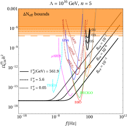
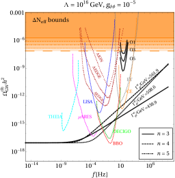
Figure 3: Same as Fig. 2, but for $\phi\to\psi\psi$ scenario. In the top left panel the vertical dashed line corresponds to $n=7/2$, for which $\beta_{\psi}=(n+4)/(n+1)$ (see text for details).

following Eq. (A), with $\beta_{\psi}=3\,(n-1)/(n+1)$. Note that, in this case, $\beta_{\psi}\gtrless(n+4)/(n+1)$ for $n\gtrless 7/2$. We see the effect of this transition in the top left panel of Fig. 3, where the evolution of the reheating temperature has different behaviour around $n=7/2$. This can be understood from Eq. (4.1.2), where, for a fixed $\Lambda$ and $g_{\psi\phi}$, one finds that

$$T_{\text{rh}}\propto\begin{cases}\frac{2^{\frac{n}{4}\,(4-n)}}{\left[\left(7-2\,n\right)\,n^{n-2}\right]^{n/2}}\,,&\,n\ll 7/2\,,\\ \left[\frac{2^{n\,(5-n)}}{n^{2\,n\,(n+1)}\,(2\,n-7)^{6\,n}}\right]^{\frac{1}{8\,n-16}}\,,&\,n\gg 7/2\,.\end{cases}$$ (72)

This shows, $T_{\text{rh}}$ decreases with $n$ for $2<n\ll 7/2$, while for $7/2\gg n<5$, an increase is observed. As before, we see from the bottom left panel, for fixed $n=3$, small couplings are disallowed from the present $\Delta N_{\text{eff}}$ constraint on $\Omega_{\text{GW}}^{(0)}$. This is understandable from Eq. (3), as for $n=3$, the GW spectral energy density behaves as $\Omega_{\text{GW}}^{(0)}\propto\left(\Lambda^{6}/g_{\psi\phi}\right)^{3/5}$, implying, a too small coupling may result in $\Omega_{\text{GW}}^{(0)}$ overproduction for a given $\Lambda$. On the other hand, it also shows that large $\Lambda$ may overproduce GW energy density for a fixed $n$ and coupling strength, as seen in the top right panel. In the bottom right panel, we show different values of $n$ that are within reach of several future experiments for $g_{\psi\phi}=10^{-5}$ and $\Lambda=10^{16}$ GeV.

4.4 Scenario III: $\phi\to aa$

The derivative interaction between inflaton and a pair of scalar bosons give rise to a decay width of

$$\Gamma_{\phi\rightarrow aa}^{e}\simeq\frac{h_{a\phi}^{2}}{3}\,\left(\frac{2}{3}\right)^{\frac{3}{2\,n}}\,\left(\frac{3\,\pi}{8}\right)^{\frac{3}{2}}\,2^{3n/2}\,\left(\frac{\Gamma\left[\frac{n+1}{2n}\right]}{\Gamma\left[\frac{1}{2n}\right]}\right)^{5}\,\frac{\Lambda^{6}}{M_{P}^{3}}\,\sum\ell^{5}\,\left|\mathcal{P}_{\ell}\right|^{2}\,,$$ (73)

with $\beta_{a}=\frac{9(n-1)}{1+n}$. In this case $\beta_{a}=(n+4)/(n+1)$ for $n=13/8$, so it is beyond our range of variation for $n$.

Figure 4: Same as Fig. 2, but for $\phi\to aa$ scenario.

Note that the $h_{a\phi}$ coupling has an inverse mass dimension. We find that for a fixed $\Lambda=10^{16}$ GeV, couplings weaker than $h_{a\phi}\lesssim 10^{-20}\,\text{GeV}^{-1}$ are entirely forbidden from present $\Delta N_{\text{eff}}$ constraint on $\Omega_{\text{GW}}^{(0)}$. This is shown via the red curve in the top left panel of Fig. 4. One can understand this behaviour from the fact that for $n>2$, smaller couplings lead to GW overproduction, as $\Omega_{\text{GW}}^{(0)}\propto h_{a\phi}^{\frac{3\,n}{1-2\,n}}$. We fix $n=5$ as a benchmark value and show the dependence of $\Omega_{\text{GW}}^{(0)}(f)$ on the scale of inflation $\Lambda$ for a given $h_{a\phi}$ in the top right panel. It is interesting to note here that the cut-off frequency $f_{\text{max}}$ is independent of the choice of the scale of inflation $\Lambda$. As mentioned, for $n>2$, one cannot go to a very small coupling since it results in GW overproduction and contradicts $\Delta N_{\text{eff}}$ bounds. This can be realized from the bottom left panel. However, for $h_{a\phi}=10^{-17}\,\text{GeV}^{-1}$ the GW amplitude falls within reach of the future detector sensitivities, still satisfying $\Delta N_{\text{eff}}$ constraint, as shown in the bottom right panel.

4.5 Combined limits

In Fig. 5, we present the parameter space that remains allowed after imposing the limits discussed in the above subsections. The red shaded regions are disallowed from BBN bound on reheating temperature, that requires $T_{\text{rh}}>4$ MeV [cf. subsection. 4.1.2], for different choices of the couplings. The “CMB bound”, shown via the gray shaded region parallel to the horizontal axes, implies bound on the scale of inflation $\Lambda\lesssim 10^{16}$ GeV, from CMB observables [cf. subsection. 4.1.3]. The cyan shaded regions are forbidden from $\Delta N_{\text{eff}}$ bound from PLANCK on overproduction of GW energy density [cf. subsection. 4.1.1]. Note that, in case of derivative interaction, the cyan region corresponds only to $h_{a\phi}=10^{-20}\,\text{GeV}^{-1}$, as for other values of $h_{a\phi}$ this bound is absent. Before moving on we would like to clarify that limits on tri-linear inflaton couplings from CMB observables have been derived in, for example, Ref. Ueno:2016dim ; Drewes:2013iaa , considering $\alpha$-attractor potential for the inflaton and taking non-perturbative effects into account. These analyses assume $n=1$ reheating scenario. We, on the other hand, are typically interested in $n>2$ in order to include bounds from $\Delta N_{\text{eff}}$, while considering only perturbative reheating.

Figure 5: $\phi\to SS$ (top left), $\phi\to\psi\psi$ (top right) and $\phi\to aa$ (bottom) scenario. In all cases the red shaded region is disallowed from BBN bound on reheating temperature $T_{\text{rh}}<4$ MeV, the cyan dashed region is forbidden from PLANCK observed $\Delta N_{\text{eff}}$ bound on GW overproduction at $f=f_{\text{max}}$, and the “CMB bound” discards scale of inflation $\Lambda>1.34\times 10^{16}$ GeV from constraint on tensor to scalar ratio.

5 UV freeze-in with time-dependent inflaton decay

In this section, we discuss Dark Matter (DM) production via UV freeze-in in a model-agnostic way, i.e., adopting the time-dependent inflaton decay rate as shown in Eq. (7). The evolution of the DM number density $n_{\text{DM}}$ is governed by the Boltzmann equation (BEQ), which can be written in a generalized form as

$$\frac{dn_{\text{DM}}}{dt}+3\,H\,n_{\text{DM}}=\gamma(T)\,,$$ (74)

where $\gamma(T)$ corresponds to the DM production rate out of SM particles as a function of the bath temperature $T$. Note that the equation (74) is coupled through $H$ to the Friedmann equation, so, in this case, we are solving the full set of equations together with Eqs. (2.1). When the SM entropy is conserved, it is instructive to rewrite Eq. (74) in terms of the DM yield defined as a ratio of DM number to entropy density of the Universe, $Y\equiv n_{\text{DM}}/s$, where $s(T)\equiv\frac{2\pi^{2}}{45}g_{\star s}(T)\,T^{3}$, with $g_{\star s}(T)$ being the number of relativistic degrees of freedom contributing to the SM entropy. Then Eq. (74) reads

$$\frac{dY}{dT}=-\frac{\gamma(T)}{H(T)\,T\,s(T)}\,.$$ (75)

For the UV freeze-in, we assume that DM communicates with the visible sector through non-renormalizable operators suppressed by an appropriate power of the scale of new physics (NP) $\Lambda_{\text{UV}}$ and that the maximal temperature of the bath is well below $\Lambda_{\text{UV}}$, so $T_{\text{max}}\ll\Lambda_{\text{UV}}$. If, in addition, we assume that the temperature of the thermal bath at the end of reheating is large enough to neglect radiation and DM masses ($m_{\text{SM}},m_{\text{DM}}\ll T_{\text{rh}}$), then the production rate of DM from the SM bath can be parametrized as Elahi:2014fsa ; Bernal:2019mhf ; Kaneta:2019zgw ; Barman:2020plp

$$\gamma(T)=\frac{T^{\kappa}}{\Lambda_{\text{UV}}^{\kappa-4}}\,,$$ (76)

where $\kappa=2\,(d-2)$ with $d$ being mass dimension of the relevant effective operator, ($d\geq 5$). Note that this scale of new physics is uncorrelated with the scale of inflation $\Lambda$ and can be larger, smaller, or equal to $\Lambda$. Finally, to match the whole observed abundance, the present DM yield $Y_{0}$ has to be fixed so that $m_{\text{DM}}\,Y_{0}=\Omega_{\text{DM}}h^{2}\frac{1}{s_{0}}\,\frac{\rho_{c}}{h^{2}}\simeq 4.3\times 10^{-10}$ GeV, where $m_{\text{DM}}$ is the DM mass in GeV, $\rho_{c}\simeq 1.1\times 10^{-5}h^{2}$ GeV/cm³ is the present critical energy density, $s_{0}\simeq 2.9\times 10^{3}$ cm^-3 is the entropy density at present, and $\Omega_{\text{DM}}h^{2}\simeq 0.12$ Planck:2018vyg .

5.1 Case-I: $T_{\text{rh}}\gg m_{\text{DM}}$

Utilizing the solutions for $T(a)$ and $H(a)$, obtained in the previous section, one finds that the DM comoving number $N\equiv n_{\text{DM}}\,a^{3}$ during the non-standard reheating evolves as

$$\frac{dN}{da}=\frac{a^{2}\,\gamma}{H}=\left[\frac{(30/\pi^{2}\,g_{\star\rho})^{\kappa/4}}{H_{e}\,\Lambda_{\text{UV}}^{\kappa-4}}\right]\,\frac{a^{\frac{5\,n+2}{n+1}}}{a_{e}^{\frac{3\,n}{n+1}}}\,\rho_{\text{SM}}(a)^{\kappa/4}\,,$$ (77)

which, after on integration between $a_{e}$ and $a_{\text{rh}}$ with the standard freeze-in initial condition $N(a_{e})=0$, leads to DM number at the end of reheating

$$N(a_{\text{rh}})\simeq a_{e}^{3}\,\frac{\left(\frac{90\,(1+\bar{w})}{\pi^{2}\,g_{\star\rho}}\,\Gamma_{\phi}^{e}\,H_{e}\,M_{P}^{2}\right)^{\frac{\kappa}{4}}}{H_{e}\,\Lambda_{\text{UV}}^{\kappa-4}}\begin{cases}\frac{1}{\zeta}\left(\frac{2}{5-3\bar{w}-2\beta}\right)^{\kappa/4}\,\left[1-\left(\frac{a_{\text{rh}}}{a_{e}}\right)^{-\zeta}\right]\,,&\beta<\frac{n+4}{n+1},\\ \Gamma\left(\frac{\kappa+4}{4},0\right)-\mathcal{I}+\left(\log\left[\frac{a_{\text{rh}}}{a_{e}}\right]\right)^{1+\frac{\kappa}{4}}\,,&\beta=\frac{n+4}{n+1},\\ \frac{1}{\xi}\left[1-\left(\frac{a_{\text{rh}}}{a_{e}}\right)^{-\xi}\right],&\beta>\frac{n+4}{n+1}\,,\end{cases}$$ (78)

where

$$\zeta\equiv\frac{\kappa\,\beta+n\left[(\beta+3)\,\kappa-24\right]-12}{4\,(n+1)}\,, \xi\equiv\frac{\kappa+(\kappa-12)\,n-6}{2\,(n+1)}\,,$$ (79)

and

$$\mathcal{I}=E_{-\frac{n}{4}}\left[\frac{n^{2}-5n-3}{n+1}\,\left(\log\left[\frac{a_{\text{rh}}}{a_{e}}\right]\right)\right]\,,$$ (80)

is the exponential integral function defined as

$$E_{i}(z)=\int_{-\infty}^{z}\,dt\,\frac{e^{t}}{t}\,,$$ (81)

whereas $\Gamma[a,z]$ is the incomplete gamma function. Note that the above result (78) is valid for light DM, i.e., with mass lower than the reheating temperature. Moreover, the UV freeze-in dark species are mainly produced just after the cosmic inflation, when the thermal bath temperature is the highest. Hence, the contribution from the late times, i.e., $a>a_{\rm rh}$, is negligible. Although the SM entropy density is not conserved when the inflaton is decaying, one can calculate the DM yield at $a_{\text{rh}}$ as $Y(a_{\text{rh}})=n_{\text{DM}}(a_{\text{rh}})/s(T_{\text{rh}})=N(a_{\text{rh}})/\left(a_{\text{rh}}^{3}\,s(T_{\text{rh}})\right)$. After the end of reheating, the SM entropy is conserved and therefore $Y(a_{\text{rh}})$ remains constant. Thus we obtain

$$Y(a_{\text{rh}})\simeq\frac{45}{2\,\pi^{2}\,g_{\star s}}\,\left(\frac{a_{e}}{a_{\text{rh}}}\right)^{3}\frac{\left(\frac{180\,n}{\pi^{2}\,g_{\star\rho}\,(n+1)}\,\Gamma_{\phi}^{e}\,H_{e}\,M_{P}^{2}\right)^{\frac{\kappa}{4}}}{H_{e}\,T_{\text{rh}}^{3}\,\Lambda_{\text{UV}}^{\kappa-4}}\begin{cases}\frac{1}{\zeta}\left(\frac{n+1}{n-\beta\,(n+1)+4}\right)^{\kappa/4}\,\left[1-\left(\frac{a_{\text{rh}}}{a_{e}}\right)^{-\zeta}\right]\,,\beta<\frac{n+4}{n+1},\\ \Gamma\left(\frac{\kappa+4}{4},0\right)-\mathcal{I}+\left(\log\left[\frac{a_{\text{rh}}}{a_{e}}\right]\right)^{1+\frac{\kappa}{4}}\,,\beta=\frac{n+4}{n+1}\,,\\ \frac{1}{\xi}\left[1-\left(\frac{a_{\text{rh}}}{a_{e}}\right)^{-\xi}\right],\beta>\frac{n+4}{n+1}\,,\end{cases}$$ (82)

where $a_{e}/a_{\text{rh}}$ can be read from Eq. (17), whereas $T_{\text{rh}}$ is given by Eq. (4.1.2). To obtain the right abundance for DM, $m_{\text{DM}}\,Y(a_{\text{rh}})$ needs to match the present DM abundance, which leads to

$$\frac{\Lambda_{\text{UV}}^{\kappa-4}}{m_{\text{DM}}}\simeq\frac{\text{GeV}^{-1}}{4.3\times 10^{-10}}\frac{45}{2\,\pi^{2}\,g_{\star s}}\,\frac{\left(\frac{180\,n}{\pi^{2}\,g_{\star\rho}\,(n+1)}\,\Gamma_{\phi}^{e}\,H_{e}\,M_{P}^{2}\right)^{\frac{\kappa}{4}}}{H_{e}\,T_{\text{rh}}^{3}}$$

$$\times\begin{cases}\frac{1}{\zeta}\left[\frac{n+1}{n-\beta\,(n+1)+4}\right]^{\frac{\kappa}{4}+\frac{3\,(n+1)}{n\,(\beta+1)-3\,n}}\,\left(1-\left(\frac{a_{\text{rh}}}{a_{e}}\right)^{-\zeta}\right)\,\left(2^{\frac{n-1}{2}}\,\frac{\Lambda^{2}\,(n+1)}{2\,M_{P}\,\Gamma_{\phi}^{e}}\right)^{\frac{3\,(n+1)}{n\,(\beta+1)-3\,n}}\,,\beta<\frac{n+4}{n+1},\\ \Gamma\left(\frac{\kappa+4}{4},0\right)-\mathcal{I}+\left(\log\left[\frac{a_{\text{rh}}}{a_{e}}\right]\right)^{1+\frac{\kappa}{4}}\,\left[\left(\frac{2^{\frac{n-1}{2}}\,(n-2)\,\Lambda^{2}}{n^{1-n}\,M_{P}\,\Gamma_{\phi}^{e}}\right)^{\frac{n+1}{2\,n-4}}\mathcal{W}^{\frac{n+1}{4-2n}}\left(\frac{2^{\frac{n-1}{2}}\,(n-2)\,\Lambda^{2}}{n^{1-n}\,M_{P}\,\Gamma_{\phi}^{e}}\right)\right]^{-3}\,,\beta=\frac{n+4}{n+1}\,,\\ \frac{1}{\xi}\,\left(1-\left(\frac{a_{\text{rh}}}{a_{e}}\right)^{-\xi}\right)\,\left[\frac{2^{\frac{n-1}{2}}\,\Lambda^{2}}{n^{1-n}\,M_{P}\,\Gamma_{\phi}^{e}}\,\frac{\beta-4+n\,(\beta-1)}{2}\right]^{\frac{3+3\,n}{4-2\,n}}\,,\beta>\frac{n+4}{n+1}\,,\end{cases}$$ (83)

which shows that for a given decay channel, and $n$, $\Lambda$ the ratio $\Lambda_{\text{UV}}^{\kappa-4}/m_{\text{DM}}$ is fixed.

5.2 Case-II: $T_{\text{rh}}\ll m_{\text{DM}}\ll T_{\text{max}}$

Production of heavy DM particles with mass exceeding the reheating temperature, is Boltzmann suppressed in the region where $m_{\text{DM}}>T_{\text{rh}}$. The present DM number density in that case could be estimated by integrating Eq. (77) from $a_{e}$ to $a_{\text{DM}}\equiv a(T=m_{\text{DM}})$, where

$$a_{\text{DM}} =a_{\text{rh}}\begin{cases}\left(\frac{T_{\text{rh}}}{m_{\text{DM}}}\right)^{\frac{4\,(n+1)}{3\,n+\beta\,(n+1)}},&\beta<\frac{n+4}{n+1}\,,\\ \frac{a_{e}}{a_{\text{rh}}}\,\exp\left(-\frac{1}{4}\,\mathcal{W}\left[-4\,\left(\frac{a_{e}}{a_{\text{rh}}}\right)^{4}\,\left(\frac{m_{\text{DM}}}{T_{\text{rh}}}\right)^{4}\,\log\left(\frac{a_{\text{rh}}}{a_{e}}\right)\right]\right),&\beta=\frac{n+4}{n+1}\,,\\ \frac{T_{\text{rh}}}{m_{\text{DM}}},&\beta>\frac{n+4}{n+1}\,.\end{cases}$$ (84)

The DM yield $Y(a_{\text{DM}})=N(a_{\text{DM}})/\left(a_{\text{DM}}^{3}\,s(m_{\text{DM}})\right)$ then reads

$$Y(a_{\text{DM}}) \simeq\frac{45}{2\,\pi^{2}\,g_{\star s}}\,\left(\frac{a_{e}}{a_{\text{DM}}}\right)^{3}\frac{\left(\frac{180\,n}{\pi^{2}\,g_{\star\rho}\,(n+1)}\,\Gamma_{\phi}^{e}\,H_{e}\,M_{P}^{2}\right)^{\frac{\kappa}{4}}}{H_{e}\,m_{\text{DM}}^{3}\,\Lambda_{\text{UV}}^{\kappa-4}}$$ (85)

$$\times\begin{cases}\frac{1}{\zeta}\left(\frac{n+1}{n-\beta(n+1)+4}\right)^{\kappa/4}\,\left[1-\left(\frac{a_{\text{DM}}}{a_{e}}\right)^{-\zeta}\right]\,,&\beta<\frac{n+4}{n+1},\\ \Gamma\left(\frac{\kappa+4}{4},0\right)-\mathcal{I}+\left(\log\left[\frac{a_{\text{DM}}}{a_{e}}\right]\right)^{1+\frac{\kappa}{4}}\,,&\beta=\frac{n+4}{n+1},\\ \frac{1}{\xi}\left[1-\left(\frac{a_{\text{DM}}}{a_{e}}\right)^{-\xi}\right],&\beta>\frac{n+4}{n+1}\,.\end{cases}$$

While the DM yield is conserved after reheating and not during reheating due to the entropy injection, the final yield at the end of reheating reads

$$Y(a_{\text{rh}})=Y(a_{\text{DM}})\,\left(\frac{a_{\text{DM}}}{a_{\text{rh}}}\right)^{3}\frac{s(a_{\text{DM}})}{s(a_{\text{rh}})}\simeq Y(a_{\text{DM}})\,\left(\frac{m_{\text{DM}}}{T_{\text{rh}}}\right)^{3}\,\left(\frac{a_{\text{DM}}}{a_{\text{rh}}}\right)^{3}\,,$$ (86)

where $a_{\text{DM}}/a_{\text{rh}}$ is given by Eq. (84). As before requiring the right abundance for the DM, one can show, for a given channel, $m_{\text{DM}}/\Lambda_{\text{UV}}^{\kappa-4}$ is a constant for a given inflaton decay channel for a fixed $n\,,\Lambda$ [cf. Eq. (5.1)]. Note that, in determining the UV freeze-in yield, we introduce three more free parameters here, namely, the DM mass $m_{\text{DM}}$, the scale of effective interaction $\Lambda_{\text{UV}}$, and the mass dimension of the DM-SM operator, $\kappa$.

5.3 Dark matter production

In Fig. 6, we show the contours that reproduce the observed DM relic abundance. We consider different reheating scenarios, e.g., $\phi\to SS\,,\psi\psi\,,aa$ and project the parameter space in $\Lambda_{\text{UV}}-m_{\text{DM}}$ plane by fixing the scale of inflation $\Lambda=10^{16}$ GeV, $n=5$ and $\kappa=6$ (or equivalently, $d=5$). We choose the strength of the inflaton-matter coupling in such a way that they give rise to observable GW spectrum as discussed in Sec. 4. From the top left panel, we first note that in all cases, the parameter space shows the existence of a cut-off for certain $m_{\text{DM}}$, beyond which DM can no longer be produced. This cut-off depends on the two cases discussed before. In case where $m_{\text{DM}}\ll T_{\text{rh}}$, DM species heavier than $T_{\text{rh}}$ cannot be created from the thermal bath due to the Boltzmann suppression. On the other hand, for dark particles with mass $T_{\text{rh}}\ll m_{\text{DM}}\ll T_{\text{max}}$, the production ceases beyond $m_{\text{DM}}=T_{\text{max}}$. In both cases, UV freeze-in production becomes inefficient when the SM temperature drops below dark matter mass. The slope of each contour is exactly given by $1/(\kappa-4)$, which can easily be obtained from Eq. (5.1) once all parameters are fixed except for $m_{\text{DM}}$ and $\Lambda_{\text{UV}}$. Next, we note that in all cases, a larger inflaton coupling $g_{i\phi}$ requires larger $\Lambda_{\text{UV}}$ to produce the correct DM abundance for a given DM mass (keeping all other parameters fixed). This can be understood from Eq. (82), where we find, for $n=5\,,\kappa=6\,,\Lambda=10^{16}$ GeV, the DM yield approximately reads $Y(a_{\text{rh}})\propto g_{S\phi}^{5/2}/\Lambda_{\text{UV}}^{2}$ in case of inflaton decaying into scalars, while for fermionic decay $Y(a_{\text{rh}})\propto g_{\psi\phi}^{3/2}/\Lambda_{\text{UV}}^{2}$ and for the derivative interaction $Y(a_{\text{rh}})\propto h_{a\phi}^{3/2}/\Lambda_{\text{UV}}^{2}$ (similar dependence can also be found from Eq. (85), for a fixed DM mass). Therefore, irrespective of the inflaton decay products, a larger coupling leads to a larger abundance that can be compensated by a higher $\Lambda_{\text{UV}}$ for a given DM mass. Moreover, for our choice of parameters, we find that the decay width into pairs of scalars is small compared to the fermionic or derivative scenario. Since the DM yield in all cases is proportional to $(\Gamma_{\phi}^{e})^{x}/\Lambda_{\text{UV}}^{\kappa-4}$ ($x$ is some function of $n$, the exact form of which depends on the decay mode), hence we see the scale $\Lambda_{\text{UV}}$ is more suppressed for the scalar case compared to other two cases.

Figure 6: Dark Matter parameter space producing right relic density in $\Lambda_{\text{UV}}-m_{\text{DM}}$ plane, considering reheating via $\phi\to SS$ (top left), $\phi\to\psi\psi$ (top right) and $\phi\to aa$ (bottom left), for a fixed $\Lambda=10^{15}$ GeV, $n=10$ and DM-SM operator of dimension $d=5$. In the bottom right panel we compare parameter space for DM -SM operators of dimension $d=\{5\,,6\,,7\}$, considering fermionic reheating as a benchmark scenario.

Figure 7: Left: Contours satisfying relic abundance for $\phi\to SS$ (black solid), $\phi\to\psi\psi$ (black dotted) and $\phi\to aa$ (black dot-dashed) scenarios. Right: GW spectrum for the three cases. We fix $\Lambda=10^{15}$ GeV and $n=10$, while choose different coupling strengths (see text).

Finally, in the bottom right panel, we show the effect of DM-SM operators of different dimensions on the DM parameter space. As an illustrative example, we choose the fermionic reheating scenario and fix all the relevant parameters. Now, we see, a larger $d\,(\equiv\kappa)$ relaxes the bound on $\Lambda_{\text{UV}}$ for a given DM mass since $Y(a_{\text{rh}})\propto m_{\text{DM}}\,\Lambda_{\text{UV}}^{8-2\,d}$. Hence, operators of larger dimensions lead to more suppression, allowing lower $\Lambda_{\text{UV}}$.

Since the same inflaton-matter coupling controls DM abundance and GW spectrum, it is, therefore, possible to make a one-to-one correspondence between DM abundance and observable PGW spectrum through such interactions. This is what is portrayed in Fig. 7. In the left panel, we show the parameter space that produces right relic abundance considering all possible inflaton-matter interactions and choosing $\{g_{S\phi}\,,g_{\psi\phi}\,,h_{a\phi}\}=\{10^{-15}\,\text{GeV}\,,10^{-7}\,,10^{-18}\,\text{GeV}^{-1}\}$, for a fixed $\Lambda_{\text{UV}}\,,n$, and considering DM-SM operator of mass dimension $d=6$. For the same choice of parameters, we show the GW spectrum in the right panel, where each curve corresponds to a range of $m_{\text{DM}}$ that gives rise to the right abundance. This shows, for the fermionic reheating scenario, that it is possible to probe the relic density allowed parameter space with GW detectors like BBO or DECIGO, for $m_{\text{DM}}\simeq\{10^{-5}-10^{11}\}$ GeV. This is also true for the bosonic (scalar) reheating scenario, where the DM mass lies in the range $m_{\text{DM}}\simeq\{10^{-5}-10^{0}\}$ GeV. Although derivative interactions can provide the right relic abundance, the prediction remains beyond the reach of future GW detectors, as shown by the black dashed curve. However, for this set of parameters, $\phi\to SS$ coupling could potentially be ruled out from future constraints on $\Delta N_{\text{eff}}$ from CMB. It is understandable that by choosing the inflaton-matter coupling and the scale of inflation appropriately, it is always possible to have a detectable GWs spectrum, satisfying BBN constraint, while accommodating the proper abundance for the DM requires tuning $\Lambda_{\text{UV}}$ and $m_{\text{DM}}$. Thus, a future GW detection can be regarded as a potential freeze-in DM signal, originating from an underlying new physics leading to a DM-SM operator of a given dimension.

6 Conclusions

This work investigates the possibility of probing inflaton couplings to the visible sector by primordial gravitational waves (GWs) of inflationary origin. We consider the inflaton field oscillating with a time-dependent amplitude assuming the $\alpha$-attractor T-model potential. Such a scenario inevitably implies a time-dependent decay width of the inflaton for potential different from quadratic (for small field strength). The inflaton is assumed to couple to a pair of bosonic or fermionic matter within a perturbative regime that can give rise to successful reheating. We then compute the primordial power spectrum and the spectral energy density of primordial GW. The energy density of the Universe turns out to be a function of the inflaton decay width at the end of inflation, which, in turn, is related to the inflaton couplings to matter. Satisfying bounds from the requirement of successful BBN and CMB, we find the inflaton coupling as small as $g_{S\phi}\sim 10^{-15}$ GeV becomes sensitive to future gravitational wave detectors in case the inflaton decays into a pair of scalar bosons via an operator of dimension three. For inflaton, Yukawa interactions with fermions, the corresponding coupling that falls within the detector sensitivity turns out to be $g_{\psi\phi}\sim 10^{-5}$. For derivative interaction involving a mass dimension five operator, coupling strength $h_{a\phi}\sim 10^{-17}\,\text{GeV}^{-1}$ becomes sensitive to the experiments. It is important to note that our result strongly depends on other free parameters of the model, for example, the shape of the potential or scale of inflation which is currently bounded from PLANCK data. However we envisage that once we got more information on inflation from next generation CMB experiments, like measuring the scale of inflation, uncertainties of our prediction would be reduced.

We finally discuss the production of dark matter (DM) during reheating from the radiation bath, assuming the DM communicates with the SM via non-renormalizable operators suppressed by large-scale $\Lambda_{\text{UV}}$. In this scenario, the UV freeze-in from the thermal bath is the primary mechanism of DM production. The freeze-in scenario requires tiny couplings between the bath and DM particles. Therefore it is very challenging if not impossible to probe such very feebly coupled dark sector. Here we promote GW as a novel observable to probe such dark sectors and identify the parameter space that satisfies the observed relic density. Because of the time-dependent inflaton decay width, the standard DM yield also gets modified in this framework. It turns out to be possible to tune the scale of new physics $\Lambda_{\text{UV}}$ and the DM mass to satisfy the PLANCK observed relic DM density. The interesting point here is that depending on the nature of the inflaton decay channel, one can produce DM over a large range of mass. As the same inflaton decay width influences DM production and controls the GW spectrum, hence a detectable GW may be interpreted as an indication of the DM detection and provide information about the scale of new physics.

Finally we comment on the fact that in our analysis we have only considered one GW detector running at a time. However once more than one GW detector starts operating then sensitivities to GW spectral shapes are expected to improve so that much larger regions of the parameter space could be probed. Such an analysis is beyond the scope of the current manuscript but we envision precision measurements that GW astronomy promises due to the planned global network of GW detectors, which can fulfill the dream of testing high-scale and weakly-coupled fundamental BSM scenarios a reality in very near future.

Appendix A Inflaton decay width calculations

In this work, the inflaton field is treated as a time-dependent external and classical background field that coherently oscillates in time. Its evolution can be parametrized by a product of a slowly varying envelope $\varphi(t)$ and a fast oscillating function $\mathcal{P}(t)$ Shtanov:1994ce ; Garcia:2020wiy ; Clery:2021bwz ,

$$\phi(t)=\varphi(t)\cdot\mathcal{P}(t).$$ (87)

The envelope is defined by the condition $\rho_{\phi}=V(\varphi)$ Shtanov:1994ce , and for the $\alpha-$attractor T model one finds

$$\varphi(t)=M_{P}\left(\frac{\rho_{\phi}(t)}{\Lambda^{4}}\right)^{\frac{1}{2n}}\,.$$ (88)

The final states are produced in a quantum process in the classical time-varying background. More specifically, we consider the transition from the vacuum, i.e., $\ket{\alpha}=\ket{0}$, to two-particle final states $\ket{\beta}=\ket{FF}$, where $F$ denotes the final state particle. The leading order S-matrix element describing this process is

$$S_{\beta\alpha}^{(1)}=-i\int d^{4}x\,\Big{\langle}\beta\Big{|}T\Big{[}\mathcal{L}_{\rm int}(x)\Big{]}\Big{|}\alpha\Big{\rangle}$$

$$=-ig_{\phi F}\int d^{4}x\,\phi(t)\cdot\Big{\langle}0\Big{|}\hat{a}_{F}(p_{1})\hat{a}_{F}(p_{2})\hat{F}\hat{F}|0\Big{\rangle}-ih_{\phi F}\int d^{4}x\,\phi(t)\cdot\Big{\langle}0\Big{|}\hat{a}_{F}(p_{1})\hat{a}_{F}(p_{2})(\partial_{\mu}\hat{F})(\partial^{\mu}\hat{F})|0\Big{\rangle}\,,$$ (89)

where $\hat{a}_{F}^{\dagger}(p_{1}),\hat{a}_{F}^{\dagger}(p_{2})$ are the creation operators for the final state particles, and $\hat{F}$ denotes the quantum field operator for the $F$ state. We will either consider contribution $\propto g_{\phi F}$ or $\propto h_{\phi F}$, but not both simultaneously. The form of $\hat{F}$ depends on the spin of $F$ particles. In what follows, we assume that the time scale of $\varphi$ variation is much longer than the time scale of interactions. Moreover, we decompose the $\mathcal{P}$ function into the Fourier modes

$$\mathcal{P}(t)=\sum_{l=-\infty}^{\infty}\mathcal{P}_{l}e^{-il\omega t},$$ (90)

with $\omega$ being the frequency of the inflaton oscillations. Hence, the S-matrix element can be written as

$$S_{\beta\alpha}^{(1)} =-ig_{F\phi}M_{P}\left(\frac{\rho_{\phi}}{\Lambda^{4}}\right)^{\frac{1}{2n}}\sum_{l}\mathcal{P}_{l}\int dt\,e^{-il\omega t}\int d^{3}x\,\Big{\langle}0\Big{|}\hat{a}_{F}(p_{1})\hat{a}_{F}(p_{2})\hat{F}\hat{F}|0\Big{\rangle}$$

$$-h_{F\phi}M_{P}\left(\frac{\rho_{\phi}}{\Lambda^{4}}\right)^{\frac{1}{2n}}\mathcal{P}_{l}\int dt\,e^{-il\omega t}\int d^{3}x\,\Big{\langle}0\Big{|}\hat{a}_{F}(p_{1})\hat{a}_{F}(p_{2})(\partial_{\mu}\hat{F})(\partial^{\mu}\hat{F})|0\Big{\rangle}$$

$$\equiv-iM_{P}\left(\frac{\rho_{\phi}}{\Lambda^{4}}\right)^{\frac{1}{2n}}\sum_{l}\mathcal{P}_{l}\times(1+\delta_{F})\mathcal{F}(F)(2\pi)^{4}\delta(l\omega-p_{1}^{0}-p_{2}^{0})\delta^{(3)}(\vec{p}_{1}+\vec{p}_{2}),$$ (91)

where $\delta_{F}=1$ for identical particles in the final state, and $\delta_{F}=0$ otherwise. The function $\mathcal{F}(F)$ depends on form of the inflaton interactions,

$$\mathcal{F}(F) =\begin{cases}g_{S\phi},&F=S,\\ g_{\psi\phi}\cdot\bar{u}^{s_{1}}(p_{1})v^{s_{2}}(p_{2}),&F=\psi,\\ g_{V\phi}\cdot g^{\mu\nu}\epsilon_{\mu}^{\sigma,*}(p_{1})\epsilon_{\nu}^{\sigma^{\prime},*}(p_{2}),&F=V,\\ h_{a\phi}\cdot(p_{1}\cdot p_{2}),&F=a,\end{cases}$$ (92)

with $\bar{u}^{s_{1}}(p_{1})$, $v^{s_{2}}(p_{2})$ denoting the Dirac spinors, and $\epsilon_{\mu}^{\sigma,*}(p_{1})$ being the polarization vectors of the gauge spin-1 field. The probability $P$ for the production of two $F$ particles with momenta $p_{1}$ and $p_{2}$ in the oscillating background of the inflaton field is given by

$$P(p_{1},p_{2}) =\frac{\big{\lvert}S_{\phi\rightarrow FF}^{(1)}\big{\rvert}^{2}}{\braket{0}{0}\braket{p_{1}}{p_{1}}\braket{p_{2}}{p_{2}}},$$ (93)

where $\braket{0}{0}=1$ and $\braket{p_{i}}{p_{i}}=(2\pi)^{3}2p_{i}^{0}\delta^{(3)}(0)$ for $i=1,2$. The modulus squared of the S-matrix element takes the form

$$\big{\lvert}S_{\phi\rightarrow FF}^{(1)}\big{\rvert}^{2} =M_{P}^{2}\left(\frac{\rho_{\phi}}{\Lambda^{4}}\right)^{\frac{1}{n}}\sum_{\rm{final}}\Big{[}\sum_{l}\mathcal{P}_{l}\times(1+\delta_{F})\mathcal{F}(F)(2\pi)^{4}\delta(l\omega-p_{1}^{0}-p_{2}^{0})\delta^{(3)}(\vec{p}_{1}+\vec{p}_{2})\Big{]}^{2},$$ (94)

where we have summed over spin/polarization states of $F$ particles. We can further simplify Eq.(94), obtaining

$$\big{\lvert}S_{\phi\rightarrow FF}^{(1)}\big{\rvert}^{2} =M_{P}^{4}\left(\frac{\rho_{\phi}}{\Lambda^{4}}\right)^{\frac{1}{n}}\sum_{l}|\mathcal{P}_{l}|^{2}(1+\delta_{F})^{2}|\overline{\mathcal{M}}^{(1)}_{\phi\rightarrow FF}|^{2}\times(2\pi)^{4}\delta(l\omega-p_{1}^{0}-p_{2}^{0})\delta^{3}(\vec{p}_{1}+\vec{p}_{2})VT.$$ (95)

The square of the dimensionless amplitude summed over spin/polarization states of particles $F$ is defined as

$$|\overline{\mathcal{M}}^{(1)}_{\phi\rightarrow FF}|^{2}\equiv\frac{1}{M_{P}^{2}}\sum_{\rm{final}}|\mathcal{F}(F)|^{2}=\begin{cases}(g_{S\phi}/M_{P})^{2},&F=S,\\ 4g_{\psi\phi}^{2}[p_{1}\cdot p_{2}-m_{\psi}^{2}]/M_{P}^{2},&F=\psi,\\ \left(\frac{g_{V\phi}}{M_{P}}\right)^{2}\left[2+\frac{(p_{1}\cdot p_{2})^{2}}{m_{V}^{4}}\right],&F=V\text{ and }m_{V}\neq 0,\\ 4\left(\frac{g_{V\phi}}{M_{P}}\right)^{2},&F=V\text{ and }m_{V}=0,\\ (h_{a\phi}/M_{P})^{2}\cdot(p_{1}\cdot p_{2})^{2}&F=a,\end{cases}$$ (96)

where

$$p_{1}\cdot p_{2}=\frac{s}{2}-m_{F}^{2},$$ (97)

with $s\equiv(p_{1}+p_{2})^{2}$ being the Mandelstam variable and $m_{\psi}$, $m_{V}$ denoting the mass of fermions and vectors in the final state, respectively. Now, the probability (Eq. (93)) takes the form

$$P(p_{1},p_{2}) =M_{P}^{4}\left(\frac{\rho_{\phi}}{\Lambda^{4}}\right)^{\frac{1}{n}}\sum_{l}\lvert\mathcal{P}_{l}\rvert^{2}\cdot(1+\delta_{F})^{2}\frac{\big{\lvert}\overline{\mathcal{M}}^{(1)}_{\phi\rightarrow FF}\big{\rvert}^{2}}{2p_{1}^{0}V\,2p_{2}^{0}V}(2\pi)^{4}\delta(l\omega-p_{1}^{0}-p_{2}^{0})\delta^{(3)}(\vec{p}_{1}+\vec{p}_{2})VT\,.$$ (98)

The total probability can then be found by summing over each outgoing momenta. In the continuum limit, this reduces to multiplying $P(p_{1},p_{1})/T$ by a factor $Vd^{3}\vec{p}_{1}/(2\pi)^{3}\,Vd^{3}\vec{p}_{2}/(2\pi)^{3}$.
The energy gain from created particles in volume $V$ and time ${\rm d}t$ is

$${\rm d}E(p_{1},p_{2})=(p_{1}^{0}+p_{2}^{0})\frac{V{\rm d}^{3}\vec{p}_{1}}{(2\pi)^{3}}\frac{V{\rm d}^{3}\vec{p}_{2}}{(2\pi)^{3}}\frac{P(p_{1},p_{1})}{T}{\rm d}t.$$ (99)

Thus, the total energy gain per volume and time for the $F$ particles is given by

$$\frac{{\rm d}E}{V{\rm d}t} =M_{P}^{4}\left(\frac{\rho_{\phi}}{\Lambda^{4}}\right)^{\frac{1}{n}}\sum_{l}\lvert\mathcal{P}_{l}\rvert^{2}\cdot(1+\delta_{F})^{2}\big{\lvert}\overline{\mathcal{M}}^{(1)}_{\phi\rightarrow FF}(k)\big{\rvert}^{2}$$

$$\times\int\frac{d^{3}\vec{p}_{1}}{(2\pi)^{3}2p_{1}^{0}}\int\frac{d^{3}\vec{p}_{2}}{(2\pi)^{3}2p_{2}^{0}}(p_{1}^{0}+p_{2}^{0})(2\pi)^{4}\delta(l\omega-p_{1}^{0}-p_{2}^{0})\delta^{3}(\vec{p}_{1}+\vec{p}_{2})$$

$$=\frac{M_{P}^{4}}{8\pi}\left(\frac{\rho_{\phi}}{\Lambda^{4}}\right)^{\frac{1}{n}}\sum_{l=1}^{\infty}l\omega\lvert\mathcal{P}_{l}\rvert^{2}\cdot(1+\delta_{F})^{2}\big{\lvert}\overline{\mathcal{M}}^{(1)}_{\phi\rightarrow FF}\big{\rvert}^{2}\sqrt{1\!-\!\frac{4m_{F}^{2}}{(l\omega)^{2}}}$$ (100)

The total energy density gained from production of $F$ particles must be compensated by the energy loss of the inflaton field, which we parametrize as $(1+\bar{w})\cdot\rho_{\phi}\Gamma_{\phi\rightarrow FF}$. Consequently, the decay width accounting for the $\phi\rightarrow FF$ interaction can be calculated from the following

$$\Gamma_{\phi\rightarrow FF} =\frac{1}{1+\bar{w}}\frac{1}{\rho_{\phi}}\frac{{\rm d}E}{V{\rm d}t}$$

$$=\frac{1}{1+\bar{w}}\frac{1}{8\pi}\frac{\omega M_{P}^{4}}{\rho_{\phi}}\left(\frac{\rho_{\phi}}{\Lambda^{4}}\right)^{\frac{1}{n}}\sum_{l=1}^{\infty}l\lvert\mathcal{P}_{l}\rvert^{2}\cdot(1+\delta_{F})^{2}\big{\lvert}\overline{\mathcal{M}}^{(1)}_{\phi\rightarrow FF}\big{\rvert}^{2}\sqrt{1\!-\!\frac{4m_{F}^{2}}{(l\omega)^{2}}}.$$ (101)

The corresponding decay widths read

$$\Gamma_{\phi\rightarrow SS} =\frac{1+n}{2n}\frac{4}{8\pi}\left(\frac{g_{S\phi}}{M_{P}}\right)^{2}\frac{\omega M_{P}^{4}}{\rho_{\phi}}\left(\frac{\rho_{\phi}}{\Lambda^{4}}\right)^{\frac{1}{n}}\sum_{l=1}^{\infty}l\lvert\mathcal{P}_{l}\rvert^{2}\sqrt{1\!-\!\frac{4m_{S}^{2}}{(l\omega)^{2}}}\,,$$

$$\Gamma_{\phi\rightarrow\psi\bar{\psi}} =\frac{1+n}{2n}\frac{1}{4\pi}\left(\frac{g_{\psi\phi}}{M_{P}}\right)^{2}\frac{\omega M_{P}^{4}}{\rho_{\phi}}\left(\frac{\rho_{\phi}}{\Lambda^{4}}\right)^{\frac{1}{n}}\sum_{l=1}^{\infty}l\lvert\mathcal{P}_{l}\rvert^{2}(l\omega)^{2}\left(1\!-\!\frac{4m_{\psi}^{2}}{(l\omega)^{2}}\right)^{3/2}\,,$$

$$\Gamma_{\phi\rightarrow VV} =\frac{1+n}{2n}\frac{1}{32\pi}\left(\frac{g_{V\phi}}{M_{P}}\right)^{2}\frac{\omega M_{P}^{4}}{\rho_{\phi}}\left(\frac{\rho_{\phi}}{\Lambda^{4}}\right)^{\frac{1}{n}}$$ (102)

$$\times\sum_{l=1}^{\infty}l\lvert\mathcal{P}_{l}\rvert^{2}\left(\frac{l\omega}{m_{V}}\right)^{4}\left[1-4\left(\frac{m_{V}}{l\omega}\right)^{2}+12\left(\frac{m_{V}}{l\omega}\right)^{4}\right]\sqrt{1\!-\!\frac{4m_{V}^{2}}{(l\omega)^{2}}}\,,$$

$$\Gamma_{\phi\rightarrow aa} =\frac{1+n}{2n}\frac{1}{8\pi}\left(\frac{h_{a\phi}}{M_{P}}\right)^{2}\frac{\omega M_{P}^{4}}{\rho_{\phi}}\left(\frac{\rho_{\phi}}{\Lambda^{4}}\right)^{\frac{1}{n}}\sum_{l=1}^{\infty}l\lvert\mathcal{P}_{l}\rvert^{2}(l\omega)^{4}\left(1-\frac{2m_{a}^{2}}{(l\omega)^{2}}\right)^{2}\sqrt{1\!-\!\frac{4m_{a}^{2}}{(l\omega)^{2}}},$$

In the limit $m_{F}\rightarrow 0$, these equations simplify

$$\Gamma_{\phi\rightarrow SS} =\frac{1+n}{2n}\frac{\omega}{2\pi}\left(\frac{g_{S\phi}M_{P}}{\Lambda^{2}}\right)^{2}\left(\frac{\rho_{\phi}}{\Lambda^{4}}\right)^{\frac{1-n}{n}}\sum_{l=1}^{\infty}l\lvert\mathcal{P}_{l}\rvert^{2}\,,$$

$$\Gamma_{\phi\rightarrow\psi\bar{\psi}} =\frac{1+n}{2n}\omega\cdot\frac{g_{\psi\phi}^{2}}{4\pi}\left(\frac{\omega M_{P}}{\Lambda^{2}}\right)^{2}\left(\frac{\rho_{\phi}}{\Lambda^{4}}\right)^{\frac{1-n}{n}}\sum_{l=1}^{\infty}l^{3}\lvert\mathcal{P}_{l}\rvert^{2}\,,$$

$$\Gamma_{\phi\rightarrow\mathcal{V}\mathcal{V}} =2\cdot\Gamma_{\phi\rightarrow SS}(g_{S\phi}\leftrightarrow g_{V\phi})\,,$$

$$\Gamma_{\phi\rightarrow aa} =\frac{1+n}{2n}\frac{\omega}{8\pi}\left(\frac{\omega^{2}M_{P}h_{a\phi}}{\Lambda^{2}}\right)^{2}\left(\frac{\rho_{\phi}}{\Lambda^{4}}\right)^{\frac{1-n}{n}}\sum_{l=1}^{\infty}l^{5}\lvert\mathcal{P}_{l}\rvert^{,},$$ (103)

where $V$ and $\mathcal{V}$ denote the massive and massless gauge fields, respectively. For the T-model, the frequency $\omega$ is related to the effective mass (23) of the inflaton field through

$$\omega=m_{\phi}\,\sqrt{\frac{\pi n}{2n-1}}\,\frac{\Gamma\left(\frac{n+1}{2n}\right)}{\Gamma\left(\frac{1}{2n}\right)}\,.$$ (104)

Its time-evolution is described by the power-law solution with the scale factor

$$\omega=\omega_{e}\cdot\left(\frac{\rho_{\phi}}{\Lambda^{4}}\right)^{\frac{n-1}{2n}}\simeq\omega_{e}\left(\frac{\rho_{e}}{\Lambda^{4}}\right)^{\frac{n-1}{2n}}\left(\frac{a_{e}}{a}\right)^{\frac{3(n-1)}{n+1}}, \omega_{e}\equiv\sqrt{2\,n^{2}\,\pi}\,\frac{\Gamma\left(\frac{n+1}{2n}\right)}{\Gamma\left(\frac{1}{2n}\right)}\,\frac{\Lambda^{2}}{M_{P}}.$$ (105)

Hence, the time dependency of the inflaton decay rate can be parametrized as

$$\Gamma_{\phi\rightarrow FF}\equiv\Gamma_{\phi\rightarrow FF}^{e}\left(\frac{a_{e}}{a}\right)^{\beta_{F}},$$ (106)

where

$$\Gamma_{\phi\rightarrow SS}^{e}=\frac{1+n}{2n}\frac{\omega_{e}}{2\pi}\left(\frac{g_{S\phi}M_{P}}{\Lambda^{2}}\right)^{2}\left(\frac{\rho_{e}}{\Lambda^{4}}\right)^{\frac{1-n}{2n}}\sum_{l=1}^{\infty}l\lvert\mathcal{P}_{l}\rvert^{2}\,,$$

$$\Gamma_{\phi\rightarrow\psi\bar{\psi}}^{e}=\omega_{e}\cdot\frac{1+n}{2n}\frac{g_{\psi\phi}^{2}}{4\pi}\left(\frac{\omega_{e}M_{P}}{\Lambda^{2}}\right)^{2}\left(\frac{\rho_{e}}{\Lambda^{4}}\right)^{\frac{n-1}{2n}}\sum_{l=1}^{\infty}l^{3}\lvert\mathcal{P}_{l}\rvert^{2}\,$$

$$\Gamma_{\phi\rightarrow\mathcal{V}\mathcal{V}}^{e}=2\cdot\Gamma_{\phi\rightarrow SS}^{e}(g_{S\phi}\leftrightarrow g_{V\phi})$$

$$\Gamma_{\phi\rightarrow aa}^{e}=\frac{1+n}{2n}\frac{\omega_{e}}{8\pi}\left(\frac{\omega_{e}^{2}M_{P}h_{a\phi}}{\Lambda^{2}}\right)^{2}\left(\frac{\rho_{e}}{\Lambda^{4}}\right)^{\frac{3n-3}{2n}}\sum_{l=1}^{\infty}l^{5}\lvert\mathcal{P}_{l}\rvert^{2},$$ (107)

and

$$\beta_{S}=\frac{3(1-n)}{1+n}, \beta_{\psi}=\frac{3(n-1)}{1+n}, \beta_{v}=\beta_{S}, \beta_{a}=\frac{9(n-1)}{1+n}\,.$$ (108)

$\begin{array}[]{|c||c|c|c|c|c|c|c|c|c|c|c|}\hline\cr n&1&2&3&4&5\\ \hline\cr\sum_{l}l|\mathcal{P}_{l}|^{2}&1/4&0.2294&0.2101&0.2177&0.2047\\ \hline\cr\sum_{l}l^{3}|\mathcal{P}_{l}|^{2}&1/4&0.2406&0.2442&0.2504&0.2571\\ \hline\cr\sum_{l}l^{5}|\mathcal{P}_{l}|^{2}&1/4&0.3433&0.5254&0.762&1.0492\\ \hline\cr\end{array}$

Table 1: Numerical values of the summation factors appearing in Eq. (107), for different values of $n$.

Appendix B Constraints on reheating from inflation

Here we derive constraints of the $\alpha$-attractor T-model from the combined WMAP, Planck, and BICEP/Keck data Planck:2018jri ; BICEP:2021xfz ; Tristram:2021tvh . Let us start with revisiting some of the necessary inflationary parameters. The so-called potential slow-roll parameters are defined as

$$\epsilon_{V}(\phi)\equiv\frac{M_{P}^{2}}{2}\,\left(\frac{V_{,\phi}(\phi)}{V(\phi)}\right)^{2}, \eta_{V}(\phi)\equiv M_{P}^{2}\frac{V_{,\phi\phi}(\phi)}{V(\phi)}\,.$$ (109)

Thus, for the $\alpha$-attractor T-model, we find

$$\epsilon_{V}^{T}(\phi)=\frac{4n^{2}}{3\alpha}\operatorname{csch}^{2}\left(\sqrt{\frac{2}{3\alpha}}\frac{\phi}{M_{P}}\right),$$ (110)

$$\eta_{V}^{T}(\phi)=\frac{4n}{3\alpha}\left[2n-\operatorname{cosh}\left(\sqrt{\frac{2}{3\alpha}}\frac{\phi}{M_{P}}\right)\right]\operatorname{csch}^{2}\left(\sqrt{\frac{2}{3\alpha}}\frac{\phi}{M_{P}}\right)\,.$$ (111)

Note that at the end of inflation $\ddot{a}=0$, which roughly corresponds to $\epsilon_{V}(\phi_{e})\simeq 1$. This condition allows us to find the inflaton field value at the end of inflation

$$\phi_{e}\simeq\sqrt{\frac{3\alpha}{2}}M_{P}\sinh^{-1}\left(\frac{2n}{\sqrt{3\alpha}}\right).$$ (112)

The inflationary number of e-folds between the horizon crossing of the perturbation with a comoving wave number $k_{\star}$ and the end of inflation is

$$N_{\star}\simeq\frac{1}{M_{P}}\int_{\phi_{e}}^{\phi_{\star}}\frac{d\phi}{\sqrt{2\epsilon_{V}^{T}(\phi)}}=\frac{3\,\alpha}{4\,n}\,\left[\cosh\left(\sqrt{\frac{2}{3\,\alpha}}\,\frac{\phi_{\star}}{M_{P}}\right)-\cosh\left(\sqrt{\frac{2}{3\,\alpha}}\,\frac{\phi_{e}}{M_{P}}\right)\right]\,,$$ (113)

with $\phi_{\star}\equiv\phi(a_{\star})$ being the field value at the moment when the Planck pivot scale $k_{\star}=0.05\,{\rm{Mpc}}^{-1}$ crosses the comoving Hubble radius, i.e., $k^{-1}_{\star}=(a_{\star}H_{\star})^{-1}$.

The two principal CMB observables, namely, the spectral index, $n_{S}$, and the tensor-to-scalar ratio, $r$, in the slow-roll approximation are defined as

$$r(\phi_{\star})=16\epsilon_{V}(\phi_{\star}), n_{S}(\phi_{\star})-1=2\eta_{V}(\phi_{\star})-6\epsilon_{V}(\phi_{\star}).$$ (114)

Using (110) and (111), we get

$$r^{T}(\phi_{\star}) =\frac{64n^{2}}{3\alpha}\operatorname{csch}^{2}\left(\sqrt{\frac{2}{3\alpha}}\frac{\phi_{\star}}{M_{P}}\right),$$ (115)

$$n_{S}^{T}(\phi_{\star})-1 =-\frac{8n}{3\alpha}\operatorname{csch}^{2}\left(\sqrt{\frac{2}{3\alpha}}\frac{\phi_{\star}}{M_{P}}\right)\left[\operatorname{cosh}\left(\sqrt{\frac{2}{3\alpha}}\frac{\phi_{\star}}{M_{P}}\right)+n\right]\,.$$ (116)

Next, one can use the above expression for the spectral tilt $n_{S}^{T}$ (116) to find the value of $\phi_{\star}$ as a function of $\alpha,n$, and $n_{S}^{T}$

$$\phi_{\star} =\sqrt{\frac{3\alpha}{2}}M_{P}\left\{-\log\left[3\alpha(1-n_{S}^{T})\right]+\log\left[4n+\sqrt{9\alpha^{2}(1-n_{S}^{T})^{2}+8n^{2}(2+3\alpha(1-n_{S}^{T}))}\right.\right.$$

$$+\left.\left.\sqrt{8n\left[n(4+3\alpha(1-n_{S}^{T}))+\left.\sqrt{8n^{2}(2+3\alpha(1-n_{S}^{T}))+9\alpha^{2}(1-n_{S}^{T})^{2}}\right)\right]}\,\right]\right\}\,.$$ (117)

The measured value of the spectral tilt $n_{S}$ by the Planck satellite for the pivot scale $k_{\star}$ is $n_{S}^{\rm{obs}}=0.9649\pm 0.0042$ Planck:2018jri . The numerical values of $\phi_{\star}$ (117) and $\phi_{e}$ (112) for different values of $n$ and fixed value of $\alpha=1/6$ are collected in Table (2).

$\begin{array}[]{|c||c|c|c|c|c|c|c|c|c|c|c|}\hline\cr n&1&2&3&4&5\\ \hline\cr\phi_{e}/M_{P}&0.88&1.21&1.41&1.56&1.67\\ \hline\cr\phi_{\star}/M_{P}&3.40&3.75&3.95&4.10&4.21\\ \hline\cr N_{\star}&56.73&56.74&56.74&56.74&56.75\\ \hline\cr\end{array}$

Table 2: Numerical values of the inflaton field amplitude and the corresponding number of e-folds $N_{\star}$ for different values of $n$ and fixed $\alpha=1/6$.

The CMB bound on $r$ allows us also to constrain the scale of inflation $\Lambda$ from above. The tensor-to-scalar ratio is defined as

$$r\equiv\frac{\Delta_{t}^{2}(k_{\star})}{\Delta_{s}^{2}(k_{\star})},$$ (118)

with

$$\Delta_{t}^{2}(k_{\star})=\frac{2}{\pi^{2}}\,\frac{H_{\star}^{2}}{M_{P}^{2}}, \Delta_{s}^{2}(k_{\star})=\frac{1}{8\pi^{2}}\,\frac{H_{\star}^{2}}{M_{P}^{2}}\frac{1}{\epsilon_{\star}},$$ (119)

denoting the dimensionless tensor and scalar power-spectra, respectively. Above, $\epsilon_{\star}\equiv-\dot{H}_{\star}/H^{2}_{\star}$ is the (Hubble) slow-roll parameter. The amplitude of the scalar power spectrum measured by Planck at $k=k_{\star}$ is $\Delta_{s}^{2}(k_{\star})=2.1\times 10^{-9}$ Planck:2018jri , which, in turn, implies $\Delta_{t}^{2}(k_{\star})\leq 6.7\times 10^{-11}$. Utilizing (119) one gets the upper bound on the Hubble rate

$$H_{\star}\simeq H_{e}\leq 4.4\times 10^{13}\,\rm{GeV},\$$ (120)

which, in turn, allow us to constraint the inflaton energy density at the end of inflation

$$\rho_{\phi}^{e}\equiv\rho_{\phi}(a_{e})=3M_{P}^{2}H_{e}^{2}\leq 3.4\times 10^{64}\,\rm{GeV^{4}}.$$ (121)

Moreover, the inflaton potential at $a=a_{\star}$ can be expressed in terms of the scalar power-spectrum and tensor-to-scalar ratio as

$$V(\phi_{\star})=\frac{3\pi^{2}}{2}M_{P}^{4}\,\Delta_{s}^{2}r,$$ (122)

which implies

$$\Lambda=\frac{M_{P}}{\tanh^{n/2}\left[\phi_{\star}/(\sqrt{6\alpha}M_{P})\right]}\cdot\left(\frac{3\pi^{2}}{2}\Delta_{s}^{2}r\right)^{1/4}$$ (123)

Since, at $a=a_{\star}$ the field value $\phi_{\star}>M_{P}$, the inflaton potential can be approximated by a constant value $V(\phi_{\star})\approx\Lambda^{4}$, which in turn sets an upper bound on the inflationary scale, $\Lambda\leq 1.34\times 10^{16}$ GeV, which has a feeble dependence on $n,\alpha$.

References

- (1) A.H. Guth, The Inflationary Universe: A Possible Solution to the Horizon and Flatness Problems, Phys. Rev. D 23 (1981) 347.
- (2) A.D. Linde, A New Inflationary Universe Scenario: A Possible Solution of the Horizon, Flatness, Homogeneity, Isotropy and Primordial Monopole Problems, Phys. Lett. B 108 (1982) 389.
- (3) M.A.G. Garcia, K. Kaneta, Y. Mambrini and K.A. Olive, Inflaton Oscillations and Post-Inflationary Reheating, JCAP 04 (2021) 012 [2012.10756].
- (4) B. Barman, N. Bernal, Y. Xu and O. Zapata, Ultraviolet freeze-in with a time-dependent inflaton decay, JCAP 07 (2022) 019 [2202.12906].
- (5) A. Ahmed, B. Grzadkowski and A. Socha, Implications of time-dependent inflaton decay on reheating and dark matter production, Phys. Lett. B 831 (2022) 137201 [2111.06065].
- (6) A. Ahmed, B. Grzadkowski and A. Socha, Higgs boson induced reheating and ultraviolet frozen-in dark matter, JHEP 02 (2023) 196 [2207.11218].
- (7) M. Giovannini, Gravitational waves constraints on postinflationary phases stiffer than radiation, Phys. Rev. D 58 (1998) 083504 [hep-ph/9806329].
- (8) M. Giovannini, Production and detection of relic gravitons in quintessential inflationary models, Phys. Rev. D 60 (1999) 123511 [astro-ph/9903004].
- (9) A. Riazuelo and J.-P. Uzan, Quintessence and gravitational waves, Phys. Rev. D 62 (2000) 083506 [astro-ph/0004156].
- (10) N. Seto and J. Yokoyama, Probing the equation of state of the early universe with a space laser interferometer, J. Phys. Soc. Jap. 72 (2003) 3082 [gr-qc/0305096].
- (11) L.A. Boyle and A. Buonanno, Relating gravitational wave constraints from primordial nucleosynthesis, pulsar timing, laser interferometers, and the CMB: Implications for the early Universe, Phys. Rev. D 78 (2008) 043531 [0708.2279].
- (12) A. Stewart and R. Brandenberger, Observational Constraints on Theories with a Blue Spectrum of Tensor Modes, JCAP 08 (2008) 012 [0711.4602].
- (13) B. Li and P.R. Shapiro, Precision cosmology and the stiff-amplified gravitational-wave background from inflation: NANOGrav, Advanced LIGO-Virgo and the Hubble tension, JCAP 10 (2021) 024 [2107.12229].
- (14) M. Artymowski, O. Czerwinska, Z. Lalak and M. Lewicki, Gravitational wave signals and cosmological consequences of gravitational reheating, JCAP 04 (2018) 046 [1711.08473].
- (15) C. Caprini and D.G. Figueroa, Cosmological Backgrounds of Gravitational Waves, Class. Quant. Grav. 35 (2018) 163001 [1801.04268].
- (16) D. Bettoni, G. Domènech and J. Rubio, Gravitational waves from global cosmic strings in quintessential inflation, JCAP 02 (2019) 034 [1810.11117].
- (17) D.G. Figueroa and E.H. Tanin, Ability of LIGO and LISA to probe the equation of state of the early Universe, JCAP 08 (2019) 011 [1905.11960].
- (18) T. Opferkuch, P. Schwaller and B.A. Stefanek, Ricci Reheating, JCAP 07 (2019) 016 [1905.06823].
- (19) N. Bernal, A. Ghoshal, F. Hajkarim and G. Lambiase, Primordial Gravitational Wave Signals in Modified Cosmologies, 2008.04959.
- (20) A. Ghoshal, L. Heurtier and A. Paul, Signatures of non-thermal dark matter with kination and early matter domination. Gravitational waves versus laboratory searches, JHEP 12 (2022) 105 [2208.01670].
- (21) R. Caldwell et al., Detection of early-universe gravitational-wave signatures and fundamental physics, Gen. Rel. Grav. 54 (2022) 156 [2203.07972].
- (22) Y. Gouttenoire, G. Servant and P. Simakachorn, Kination cosmology from scalar fields and gravitational-wave signatures, 2111.01150.
- (23) V.K. Oikonomou, Effects of the axion through the higgs portal on primordial gravitational waves during the electroweak breaking, Phys. Rev. D 107 (2023) 064071.
- (24) G. Jungman, M. Kamionkowski and K. Griest, Supersymmetric dark matter, Phys. Rept. 267 (1996) 195 [hep-ph/9506380].
- (25) G. Bertone, D. Hooper and J. Silk, Particle dark matter: Evidence, candidates and constraints, Phys. Rept. 405 (2005) 279 [hep-ph/0404175].
- (26) J.L. Feng, Dark Matter Candidates from Particle Physics and Methods of Detection, Ann. Rev. Astron. Astrophys. 48 (2010) 495 [1003.0904].
- (27) L. Roszkowski, E.M. Sessolo and S. Trojanowski, WIMP dark matter candidates and searches—current status and future prospects, Rept. Prog. Phys. 81 (2018) 066201 [1707.06277].
- (28) G. Arcadi, M. Dutra, P. Ghosh, M. Lindner, Y. Mambrini, M. Pierre et al., The waning of the WIMP? A review of models, searches, and constraints, Eur. Phys. J. C 78 (2018) 203 [1703.07364].
- (29) J. McDonald, Thermally generated gauge singlet scalars as selfinteracting dark matter, Phys.Rev.Lett. 88 (2002) 091304 [hep-ph/0106249].
- (30) L.J. Hall, K. Jedamzik, J. March-Russell and S.M. West, Freeze-In Production of FIMP Dark Matter, JHEP 03 (2010) 080 [0911.1120].
- (31) N. Bernal, M. Heikinheimo, T. Tenkanen, K. Tuominen and V. Vaskonen, The Dawn of FIMP Dark Matter: A Review of Models and Constraints, Int. J. Mod. Phys. A32 (2017) 1730023 [1706.07442].
- (32) F. Elahi, C. Kolda and J. Unwin, UltraViolet Freeze-in, JHEP 03 (2015) 048 [1410.6157].
- (33) R.T. Co, E. Gonzalez and K. Harigaya, Increasing Temperature toward the Completion of Reheating, JCAP 11 (2020) 038 [2007.04328].
- (34) A. Banerjee and D. Chowdhury, Fingerprints of freeze-in dark matter in an early matter-dominated era, SciPost Phys. 13 (2022) 022 [2204.03670].
- (35) R. Kallosh and A. Linde, Universality Class in Conformal Inflation, JCAP 07 (2013) 002 [1306.5220].
- (36) G.F. Giudice, E.W. Kolb and A. Riotto, Largest temperature of the radiation era and its cosmological implications, Phys. Rev. D 64 (2001) 023508 [hep-ph/0005123].
- (37) K. Ichikawa, T. Suyama, T. Takahashi and M. Yamaguchi, Primordial Curvature Fluctuation and Its Non-Gaussianity in Models with Modulated Reheating, Phys. Rev. D 78 (2008) 063545 [0807.3988].
- (38) K. Kainulainen, S. Nurmi, T. Tenkanen, K. Tuominen and V. Vaskonen, Isocurvature Constraints on Portal Couplings, JCAP 06 (2016) 022 [1601.07733].
- (39) S. Clery, Y. Mambrini, K.A. Olive and S. Verner, Gravitational portals in the early Universe, Phys. Rev. D 105 (2022) 075005 [2112.15214].
- (40) R.T. Co, Y. Mambrini and K.A. Olive, Inflationary Gravitational Leptogenesis, 2205.01689.
- (41) A. Ahmed, B. Grzadkowski and A. Socha, Higgs Boson-Induced Reheating and Dark Matter Production, Symmetry 14 (2022) 306.
- (42) L.A. Boyle and P.J. Steinhardt, Probing the early universe with inflationary gravitational waves, Phys. Rev. D 77 (2008) 063504 [astro-ph/0512014].
- (43) Y. Watanabe and E. Komatsu, Improved Calculation of the Primordial Gravitational Wave Spectrum in the Standard Model, Phys. Rev. D 73 (2006) 123515 [astro-ph/0604176].
- (44) K. Saikawa and S. Shirai, Primordial gravitational waves, precisely: The role of thermodynamics in the Standard Model, JCAP 05 (2018) 035 [1803.01038].
- (45) J. Ghiglieri and M. Laine, Gravitational wave background from Standard Model physics: Qualitative features, JCAP 07 (2015) 022 [1504.02569].
- (46) M. Maggiore, Gravitational wave experiments and early universe cosmology, Phys. Rept. 331 (2000) 283 [gr-qc/9909001].
- (47) S. Kuroyanagi, T. Chiba and N. Sugiyama, Precision calculations of the gravitational wave background spectrum from inflation, Phys. Rev. D 79 (2009) 103501 [0804.3249].
- (48) R. Allahverdi et al., The First Three Seconds: a Review of Possible Expansion Histories of the Early Universe, 2006.16182.
- (49) G. Choi, R. Jinno and T.T. Yanagida, Probing PeV scale SUSY breaking with satellite galaxies and primordial gravitational waves, Phys. Rev. D 104 (2021) 095018 [2107.12804].
- (50) D.G. Figueroa and E.H. Tanin, Inconsistency of an inflationary sector coupled only to Einstein gravity, JCAP 10 (2019) 050 [1811.04093].
- (51) S. Dodelson and M.S. Turner, Nonequilibrium neutrino statistical mechanics in the expanding universe, Phys. Rev. D 46 (1992) 3372.
- (52) S. Hannestad and J. Madsen, Neutrino decoupling in the early universe, Phys. Rev. D 52 (1995) 1764 [astro-ph/9506015].
- (53) A.D. Dolgov, S.H. Hansen and D.V. Semikoz, Nonequilibrium corrections to the spectra of massless neutrinos in the early universe, Nucl. Phys. B 503 (1997) 426 [hep-ph/9703315].
- (54) G. Mangano, G. Miele, S. Pastor, T. Pinto, O. Pisanti and P.D. Serpico, Relic neutrino decoupling including flavor oscillations, Nucl. Phys. B 729 (2005) 221 [hep-ph/0506164].
- (55) P.F. de Salas and S. Pastor, Relic neutrino decoupling with flavour oscillations revisited, JCAP 07 (2016) 051 [1606.06986].
- (56) M. Escudero Abenza, Precision early universe thermodynamics made simple: and neutrino decoupling in the Standard Model and beyond, JCAP 05 (2020) 048 [2001.04466].
- (57) K. Akita and M. Yamaguchi, A precision calculation of relic neutrino decoupling, JCAP 08 (2020) 012 [2005.07047].
- (58) J. Froustey, C. Pitrou and M.C. Volpe, Neutrino decoupling including flavour oscillations and primordial nucleosynthesis, JCAP 12 (2020) 015 [2008.01074].
- (59) J.J. Bennett, G. Buldgen, P.F. De Salas, M. Drewes, S. Gariazzo, S. Pastor et al., Towards a precision calculation of in the Standard Model II: Neutrino decoupling in the presence of flavour oscillations and finite-temperature QED, JCAP 04 (2021) 073 [2012.02726].
- (60) S. Kuroyanagi, T. Takahashi and S. Yokoyama, Blue-tilted Tensor Spectrum and Thermal History of the Universe, JCAP 02 (2015) 003 [1407.4785].
- (61) Planck collaboration, Planck 2018 results. VI. Cosmological parameters, Astron. Astrophys. 641 (2020) A6 [1807.06209].
- (62) T.-H. Yeh, J. Shelton, K.A. Olive and B.D. Fields, Probing Physics Beyond the Standard Model: Limits from BBN and the CMB Independently and Combined, 2207.13133.
- (63) K. Abazajian et al., CMB-S4 Science Case, Reference Design, and Project Plan, 1907.04473.
- (64) CMB-HD collaboration, Snowmass2021 CMB-HD White Paper, 2203.05728.
- (65) COrE collaboration, COrE (Cosmic Origins Explorer) A White Paper, 1102.2181.
- (66) EUCLID collaboration, Euclid Definition Study Report, 1110.3193.
- (67) S. Sarkar, Big bang nucleosynthesis and physics beyond the standard model, Rept. Prog. Phys. 59 (1996) 1493 [hep-ph/9602260].
- (68) M. Kawasaki and T. Moroi, Gravitino production in the inflationary universe and the effects on big bang nucleosynthesis, Prog. Theor. Phys. 93 (1995) 879 [hep-ph/9403364].
- (69) M. Kawasaki, K. Kohri and N. Sugiyama, MeV scale reheating temperature and thermalization of neutrino background, Phys. Rev. D 62 (2000) 023506 [astro-ph/0002127].
- (70) S. Hannestad, What is the lowest possible reheating temperature?, Phys. Rev. D 70 (2004) 043506 [astro-ph/0403291].
- (71) F. De Bernardis, L. Pagano and A. Melchiorri, New constraints on the reheating temperature of the universe after WMAP-5, Astropart. Phys. 30 (2008) 192.
- (72) P. de Salas, M. Lattanzi, G. Mangano, G. Miele, S. Pastor and O. Pisanti, Bounds on very low reheating scenarios after Planck, Phys. Rev. D 92 (2015) 123534 [1511.00672].
- (73) T. Hasegawa, N. Hiroshima, K. Kohri, R.S.L. Hansen, T. Tram and S. Hannestad, MeV-scale reheating temperature and thermalization of oscillating neutrinos by radiative and hadronic decays of massive particles, JCAP 12 (2019) 012 [1908.10189].
- (74) M.R. Haque and D. Maity, Gravitational Reheating, 2201.02348.
- (75) S. Clery, Y. Mambrini, K.A. Olive, A. Shkerin and S. Verner, Gravitational portals with nonminimal couplings, Phys. Rev. D 105 (2022) 095042 [2203.02004].
- (76) M.R. Haque, D. Maity and R. Mondal, WIMPs, FIMPs, and Inflaton phenomenology via reheating, CMB and , 2301.01641.
- (77) R. Brandenberger, V. Kamali and R. O. Ramos, Minimal Preheating, 2305.11246.
- (78) L. Kofman, A.D. Linde and A.A. Starobinsky, Reheating after inflation, Phys. Rev. Lett. 73 (1994) 3195 [hep-th/9405187].
- (79) L. Kofman, A.D. Linde and A.A. Starobinsky, Towards the theory of reheating after inflation, Phys. Rev. D 56 (1997) 3258 [hep-ph/9704452].
- (80) M.A.G. Garcia and M. Pierre, Reheating after Inflaton Fragmentation, 2306.08038.
- (81) D.G. Figueroa and F. Torrenti, Gravitational wave production from preheating: parameter dependence, JCAP 10 (2017) 057 [1707.04533].
- (82) C. Cosme, D.G. Figueroa and N. Loayza, Gravitational wave production from preheating with trilinear interactions, JCAP 05 (2023) 023 [2206.14721].
- (83) K. Schmitz, New Sensitivity Curves for Gravitational-Wave Experiments, 2002.04615.
- (84) LIGO Scientific, Virgo collaboration, Observation of Gravitational Waves from a Binary Black Hole Merger, Phys. Rev. Lett. 116 (2016) 061102 [1602.03837].
- (85) LIGO Scientific, Virgo collaboration, GW151226: Observation of Gravitational Waves from a 22-Solar-Mass Binary Black Hole Coalescence, Phys. Rev. Lett. 116 (2016) 241103 [1606.04855].
- (86) LIGO Scientific, VIRGO collaboration, GW170104: Observation of a 50-Solar-Mass Binary Black Hole Coalescence at Redshift 0.2, Phys. Rev. Lett. 118 (2017) 221101 [1706.01812].
- (87) LIGO Scientific, Virgo collaboration, GW170608: Observation of a 19-solar-mass Binary Black Hole Coalescence, Astrophys. J. Lett. 851 (2017) L35 [1711.05578].
- (88) LIGO Scientific, Virgo collaboration, GW170814: A Three-Detector Observation of Gravitational Waves from a Binary Black Hole Coalescence, Phys. Rev. Lett. 119 (2017) 141101 [1709.09660].
- (89) LIGO Scientific, Virgo collaboration, GW170817: Observation of Gravitational Waves from a Binary Neutron Star Inspiral, Phys. Rev. Lett. 119 (2017) 161101 [1710.05832].
- (90) LISA collaboration, Laser Interferometer Space Antenna, arXiv e-prints (2017) arXiv:1702.00786 [1702.00786].
- (91) J. Baker et al., The Laser Interferometer Space Antenna: Unveiling the Millihertz Gravitational Wave Sky, 1907.06482.
- (92) LIGO Scientific collaboration, Exploring the Sensitivity of Next Generation Gravitational Wave Detectors, Class. Quant. Grav. 34 (2017) 044001 [1607.08697].
- (93) D. Reitze et al., Cosmic Explorer: The U.S. Contribution to Gravitational-Wave Astronomy beyond LIGO, Bull. Am. Astron. Soc. 51 (2019) 035 [1907.04833].
- (94) M. Punturo et al., The Einstein Telescope: A third-generation gravitational wave observatory, Class. Quant. Grav. 27 (2010) 194002.
- (95) S. Hild et al., Sensitivity Studies for Third-Generation Gravitational Wave Observatories, Class. Quant. Grav. 28 (2011) 094013 [1012.0908].
- (96) J. Crowder and N.J. Cornish, Beyond LISA: Exploring future gravitational wave missions, Phys. Rev. D 72 (2005) 083005 [gr-qc/0506015].
- (97) V. Corbin and N.J. Cornish, Detecting the cosmic gravitational wave background with the big bang observer, Class. Quant. Grav. 23 (2006) 2435 [gr-qc/0512039].
- (98) N. Seto, S. Kawamura and T. Nakamura, Possibility of direct measurement of the acceleration of the universe using 0.1-Hz band laser interferometer gravitational wave antenna in space, Phys. Rev. Lett. 87 (2001) 221103 [astro-ph/0108011].
- (99) H. Kudoh, A. Taruya, T. Hiramatsu and Y. Himemoto, Detecting a gravitational-wave background with next-generation space interferometers, Phys. Rev. D 73 (2006) 064006 [gr-qc/0511145].
- (100) K. Nakayama and J. Yokoyama, Gravitational Wave Background and Non-Gaussianity as a Probe of the Curvaton Scenario, JCAP 01 (2010) 010 [0910.0715].
- (101) K. Yagi and N. Seto, Detector configuration of DECIGO/BBO and identification of cosmological neutron-star binaries, Phys. Rev. D 83 (2011) 044011 [1101.3940].
- (102) S. Kawamura et al., Current status of space gravitational wave antenna DECIGO and B-DECIGO, PTEP 2021 (2021) 05A105 [2006.13545].
- (103) A. Sesana et al., Unveiling the gravitational universe at -Hz frequencies, Exper. Astron. 51 (2021) 1333 [1908.11391].
- (104) A. Vallenari, The future of astrometry in space, Frontiers in Astronomy and Space Sciences 5 (2018) .
- (105) AEDGE collaboration, AEDGE: Atomic Experiment for Dark Matter and Gravity Exploration in Space, EPJ Quant. Technol. 7 (2020) 6 [1908.00802].
- (106) L. Badurina, O. Buchmueller, J. Ellis, M. Lewicki, C. McCabe and V. Vaskonen, Prospective sensitivities of atom interferometers to gravitational waves and ultralight dark matter, Phil. Trans. A. Math. Phys. Eng. Sci. 380 (2021) 20210060 [2108.02468].
- (107) P.W. Graham, J.M. Hogan, M.A. Kasevich and S. Rajendran, Resonant mode for gravitational wave detectors based on atom interferometry, Phys. Rev. D 94 (2016) 104022 [1606.01860].
- (108) MAGIS collaboration, Mid-band gravitational wave detection with precision atomic sensors, 1711.02225.
- (109) L. Badurina et al., AION: An Atom Interferometer Observatory and Network, JCAP 05 (2020) 011 [1911.11755].
- (110) Y. Ueno and K. Yamamoto, Constraints on -attractor inflation and reheating, Phys. Rev. D 93 (2016) 083524 [1602.07427].
- (111) M. Drewes and J.U. Kang, The Kinematics of Cosmic Reheating, Nucl. Phys. B 875 (2013) 315 [1305.0267].
- (112) D. Chowdhury and A. Hait, Thermalization in the presence of a time-dependent dissipation and its impact on dark matter production, 2302.06654.
- (113) N. Bernal, F. Elahi, C. Maldonado and J. Unwin, Ultraviolet Freeze-in and Non-Standard Cosmologies, JCAP 1911 (2019) 026 [1909.07992].
- (114) K. Kaneta, Y. Mambrini and K.A. Olive, Radiative production of nonthermal dark matter, Phys. Rev. D 99 (2019) 063508 [1901.04449].
- (115) B. Barman, D. Borah and R. Roshan, Effective Theory of Freeze-in Dark Matter, 2007.08768.
- (116) A. Chakraborty, M.R. Haque, D. Maity and R. Mondal, Inflaton phenomenology via reheating in the light of PGWs and latest BICEP/ data, 2304.13637.
- (117) Y. Shtanov, J.H. Traschen and R.H. Brandenberger, Universe reheating after inflation, Phys. Rev. D 51 (1995) 5438 [hep-ph/9407247].
- (118) Planck collaboration, Planck 2018 results. X. Constraints on inflation, Astron. Astrophys. 641 (2020) A10 [1807.06211].
- (119) BICEP, Keck collaboration, Improved Constraints on Primordial Gravitational Waves using Planck, WMAP, and BICEP/Keck Observations through the 2018 Observing Season, Phys. Rev. Lett. 127 (2021) 151301 [2110.00483].
- (120) M. Tristram et al., Improved limits on the tensor-to-scalar ratio using BICEP and Planck data, Phys. Rev. D 105 (2022) 083524 [2112.07961].