Kullback-Leibler Maillard Sampling for Multi-armed Bandits with Bounded Rewards

Abstract

We study $K$-armed bandit problems where the reward distributions of the arms are all supported on the $[0,1]$ interval. Maillard sampling [31], an attractive alternative to Thompson sampling, has recently been shown to achieve competitive regret guarantees in the sub-Gaussian reward setting [11] while maintaining closed-form action probabilities, which is useful for offline policy evaluation. In this work, we analyze the Kullback-Leibler Maillard Sampling (KL-MS) algorithm, a natural extension of Maillard sampling and a special case of Minimum Empirical Divergence (MED) [20] for achieving a KL-style finite-time gap-dependent regret bound. We show that KL-MS enjoys the asymptotic optimality when the rewards are Bernoulli and has an adaptive worst-case regret bound of the form $O(\sqrt{\mu^{*}(1-\mu^{*})KT\ln K}+K\ln T)$, where $\mu^{*}$ is the expected reward of the optimal arm, and $T$ is the time horizon length; this is the first time such adaptivity is reported in the literature for an algorithm with asymptotic optimality guarantees.

1 Introduction

The multi-armed bandit (abbrev. MAB) problem [42, 28, 30], a stateless version of the reinforcement learning problem, has received much attention by the research community, due to its relevance in may applications such as online advertising, recommendation, and clinical trials. In a multi-armed bandit problem, a learning agent has access to a set of $K$ arms (also known as actions), where for each $i\in[K]\mathrel{\mathop{\mathchar 58\relax}}=\mathinner{\left\{1,\ldots,K\right\}}$, arm $i$ is associated with a distribution $\nu_{i}$ with mean $\mu_{i}$; at each time step $t$, the agent adaptively chooses an arm $I_{t}\in[K]$ by sampling from a probability distribution $p_{t}\in\Delta^{K-1}$ and receives reward $y_{t}\sim\nu_{I_{t}}$, based on the information the agent has so far. The goal of the agent is to minimize its pseudo-regret over $T$ time steps: $\mathrm{Reg}(T)=T\mu^{*}-\mathbb{E}\sum_{t=1}^{T}y_{t}$, where $\mu^{*}=\max_{i}\mu_{i}$ is the optimal expected reward.

In this paper, we study the multi-armed bandit setting where reward distributions of all arms are supported on $[0,1]$. An important special case is Bernoulli bandits, where for each arm $i$, $\nu_{i}=\mathrm{Bernoulli}(\mu_{i})$ for some $\mu_{i}\in[0,1]$. It has practical relevance in settings such as computational advertising, where the reward feedback is oftentimes binary (click vs. not-click, buy vs. not-buy).

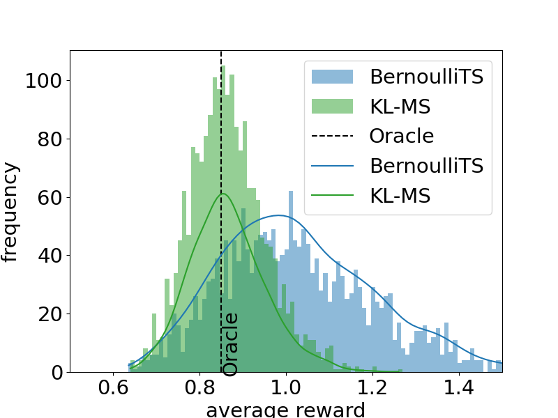
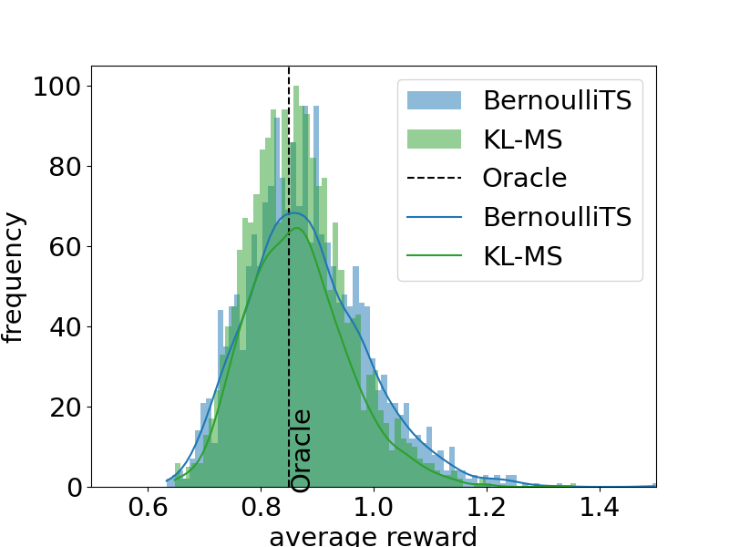
Broadly speaking, there are two popular families of provably regret-efficient algorithms for bounded-reward bandit problems: deterministic exploration algorithms (such as KL-UCB [17, 13, 32]) and randomized exploration algorithms (such as Thompson sampling (TS) [42]). Randomized exploration algorithms such as TS have been very popular, perhaps due to its excellent empirical performance and the ability to cope with delayed rewards better than deterministic counterparts [15]. In addition, the logged data collected from randomized exploration, of the form $(I_{t},p_{t,I_{t}},y_{t})_{t=1}^{T}$, where $p_{t,I_{t}}$ is the probability with which arm $I_{t}$ was chosen, are useful for offline evaluation purposes by employing the inverse propensity weighting (IPW) estimator [23] or the doubly robust estimator [39]. However, calculating the arm sampling probability distribution $p_{t}$ for Thompson sampling is nontrivial. Specifically, there is no known closed-form , and generic numerical integration methods and Monte-Carlo approximations suffer from instability issues: the time complexity for obtaining a numerical precision of $\epsilon$ is $\Omega(\mathrm{poly}(1/\epsilon))$ [37]. This is too slow to be useful especially for web-scale deployments; e.g., Google AdWords receives $\sim$237M clicks per day. Furthermore, the computed probability will be used after taking the inversion, which means that even moderate amount of errors are intolerable. Indeed, Figure 1 shows that the offline evaluation with Thompson sampling as the behavioral policy will be largely biased and inaccurate due to the errors from the Monte Carlo approximation.

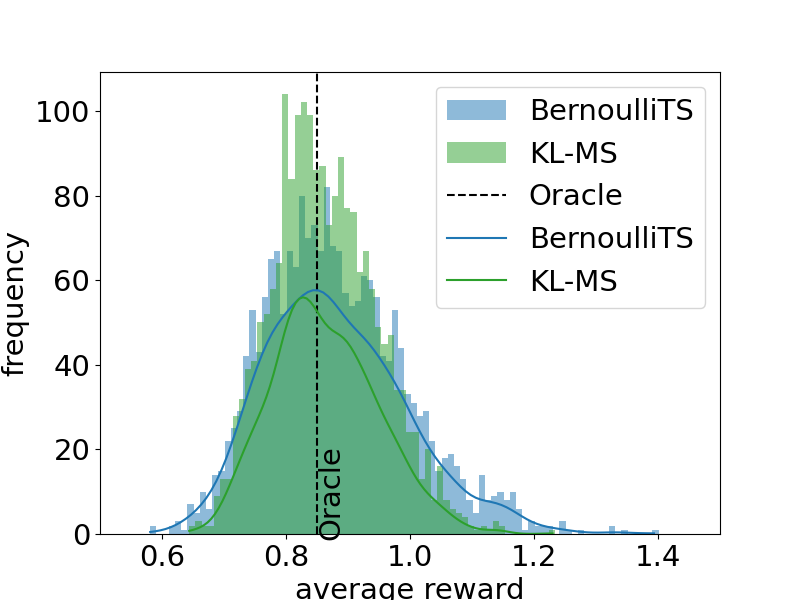
Figure 1: Histogram of the average rewards computed from the offline evaluation where the logged data is collected from Bernoulli TS and KL-MS (Algorithm 1) in a Bernoulli bandit environment with the mean reward (0.8, 0.9) with time horizon $T=10,000$. For Bernoulli TS’s log, we approximate the action probability by Monte Carlo Sampling with 1000 samples for each step. Here we estimate the expected reward of the uniform policy which has expected average reward of 0.85 (black dashed line). Across 2000 trials, the logged data of KL-MS induces an MSE of $0.00796$; however, for half of the trials, the IPW estimator induced by Bernoulli TS’s log returns invalid values due to the action probability estimates being zero. Even excluding those invalid values, the Bernoulli TS’s logged data induces an MSE of $0.02015$. See Appendix H for additional experiments.

Recently, many studies have introduced alternative randomized algorithms that allow an efficient computation of $p_{t}$ [20, 31, 14, 44]. Of these, Maillard sampling (MS)  [31, 11], a Gaussian adaptation of the Minimum Empirical Divergence (MED) algorithm [20] originally designed for finite-support reward distributions, provides a simple algorithm for the sub-Gaussian bandit setting that computes $p_{t}$ in a closed form:

$$p_{t,a}\propto\exp\mathinner{\left(-N_{t-1,a}{\frac{\hat{\Delta}_{t-1,a}^{2}}{2\sigma^{2}}}\right)}$$ (1)

where at time step $t$, $N_{t,a}$ is the number of pulling arm $a$. We define the estimator of $\mu_{a}$ as ${\hat{\mu}}_{t,a}\mathrel{\mathop{\mathchar 58\relax}}=\frac{\sum_{s=1}^{t}{\bf 1}\mathinner{\left\{I_{t}=a\right\}}y_{t}}{N_{t,a}}$ and the best performed mean value as ${\hat{\mu}}_{t,\max}\mathrel{\mathop{\mathchar 58\relax}}=\max_{a\in[K]}\mu_{t,a}$. $\hat{\Delta}_{t-1,a}=\max_{a^{\prime}}{\hat{\mu}}_{t-1,a^{\prime}}-{\hat{\mu}}_{t-1,a}$ is the empirical suboptimality gap of arm $a$, and $\sigma$ is the subgaussian parameter of the reward distribution of all arms. For sub-Gaussian reward distributions, MS enjoys the asymptotic optimality under the special case of Gaussian rewards and a near-minimax optimality [11], making it an attractive alternative to Thompson sampling. Also, MS satisfies the sub-UCB criterion (see Section 2 for a precise definition) to help establish sharp finite-time instance-dependent regret guarantees. Can we adapt MS to the bounded reward setting and achieve the asymptotic, minimax optimality and sub-UCB criterion while computing the sampling probability in a closed-form? In this paper, we make significant progress on this question.

Our contributions.

We focus on a Bernoulli adaptation of MS that we call Kullback-Leibler Maillard Sampling (abbrev. KL-MS) and perform a finite-time analysis of it in the bounded-reward bandit problem. KL-MS uses a sampling probability similar to MS but tailored to the $[0,1]$-bounded reward setting:

$$p_{t,a}\propto\exp\mathinner{\left(-N_{t-1,a}\mathsf{kl}\mathinner{\left({\hat{\mu}}_{t-1,a},{\hat{\mu}}_{t-1,\max}\right)}\right)},$$

where $\mathsf{kl}(\mu,\mu^{\prime})\mathrel{\mathop{\mathchar 58\relax}}=\mu\ln\frac{\mu}{\mu^{\prime}}+(1-\mu)\ln\frac{1-\mu}{1-\mu^{\prime}}$ is the binary Kullback-Leibler (KL) divergence. We can also view KL-MS as an instantiation of MED [20] for Bernoulli rewards; See Section 3 for a detailed comparison.

KL-MS performs an efficient exploration for bounded rewards since one can use $\mathsf{kl}(a,b)\geq 2(a-b)^{2}$ to verify that the probability being assigned to each empirical non-best arm by KL-MS is never larger than that of MS with $\sigma^{2}=1/4$, the best sub-Gaussian parameter for the bounded rewards in $[0,1]$. We show that KL-MS achieves a sharp finite-time regret guarantee (Theorem 1) that can be simultaneously converted to:

• an asymptotic regret upper bound (Theorem 4), which is asymptotically optimal when specialized to the Bernoulli bandit setting;

• a $\sqrt{T}$-style regret guarantee of $O(\sqrt{\mu^{*}(1-\mu^{*})KT\ln K}+K\ln(T))$ (Theorem 3) where $\mu^{*}$ is the mean reward of the best arm. This bound has two salient features. First, in the worst case, it is at most a $\sqrt{\ln K}$ factor suboptimal than the minimax optimal regret of $\Theta(\sqrt{KT})$ [5, 10]. Second, its $\tilde{O}(\sqrt{\mu^{*}(1-\mu^{*})}$ coefficient adapts to the variance of the optimal arm reward; this is the first time such adaptivity is reported in the literature for an algorithm with asymptotical optimality guarantees.

• a sub-UCB regret guarantee, which many existing minimax optimal algorithms [34, 18] have not been proven to satisfy.

Algorithm&	Finite-Time Regret		Closed-form	Reference
Analysis	Minimax Ratio	Sub-UCB	Probability
TS	$\sqrt{\ln K}$	yes	no	See the caption
ExpTS	$\sqrt{\ln K}$	yes	no	Jin et al. [25]
$\text{ ExpTS}^{+}$	$1$	$-^{\star\star}$	no	Jin et al. [25]
kl-UCB	$\sqrt{\ln T}$	yes	N/A	Cappé et al. [13]
kl-UCB++	$1$	$-^{\star\star}$	N/A	Ménard and Garivier [34]
kl-UCB-switch	$1$	$-^{\star\star}$	N/A	Garivier et al. [18]
MED	$-$	$-$	$\text{no}^{\star}$	Honda and Takemura [20]
DMED	$-$	$-$	N/A	Honda and Takemura [21]
IMED	$-$	$-$	N/A	Honda and Takemura [22]
KL-MS	$\sqrt{\ln K}$	yes	yes	this paper

Table 1: Comparison of regret bounds for bounded reward distributions; for space constraints we only include those that achieves the asymptotic optimality for the special case of Bernoulli distributions (this excludes, e.g., Maillard Sampling [31, 11], Tsallis-INF [44] and UCB-V [8]). ‘$-$’indicates that the corresponding analysis is not reported. ‘N/A’indicates that the algorithm does have closed-form, but it is deterministic. ‘$\star$’indicates that its computational complexity for calculating the action probability is $\ln(1/\text{precision})$. ‘$\star\star$’indicates that we conjecture that the algorithm is not sub-UCB. The results on TS are reported by Agrawal and Goyal [3, 4], Korda et al. [27].

We also conduct experiments that show that thanks to its closed-form action probabilities, KL-MS generates much more reliable logged data than Bernoulli TS with Monte Carlo estimation of action probabilities; this is reflected in their offline evaluation performance using the IPW estimator; see Figure 1 and Appendix H for more details.

2 Preliminaries

Let $N_{t,a}$ be the number of times arm $a$ has been pulled until time step $t$ (inclusively). Denote the suboptimality gap of arm $a$ by $\Delta_{a}\mathrel{\mathop{\mathchar 58\relax}}=\mu^{*}-\mu_{a}$, where $\mu^{*}=\max_{i\in[K]}\mu_{i}$ is the optimal expected reward. Denote the empirical suboptimality gap of arm $a$ by $\hat{\Delta}_{t,a}\mathrel{\mathop{\mathchar 58\relax}}=\hat{\mu}_{t,\max}-\hat{\mu}_{t,a}$; here, $\hat{\mu}_{t,a}$ is the empirical estimation to $\mu_{a}$ up to time step $t$, i.e., $\hat{\mu}_{t,a}\mathrel{\mathop{\mathchar 58\relax}}=\frac{1}{N_{t,a}}\sum_{s=1}^{t}y_{s}{\bf 1}\mathinner{\left\{I_{s}=a\right\}}$, and $\hat{\mu}_{t,\max}=\max_{a\in[K]}{\hat{\mu}}_{t,a}$ is the best empirical reward at time step $t$. For arm $a$, define $\tau_{a}(s)\mathrel{\mathop{\mathchar 58\relax}}=\min\mathinner{\left\{t\geq 1\mathrel{\mathop{\mathchar 58\relax}}N_{t,a}=s\right\}}$ at the time step when arm $a$ is pulled for the $s$-th time, which is a stopping time; we also use $\hat{\mu}_{(s),a}\mathrel{\mathop{\mathchar 58\relax}}=\hat{\mu}_{\tau_{a}(s),a}$ to denote empirical mean of the first $s$ reward values received from pulling arm $a$.

We define the Kullback-Leibler divergence between two distributions $\nu$ and $\rho$ as ${\mathsf{KL}}(\nu,\rho)=\mathbb{E}_{X\sim\nu}\mathinner{\left[\ln\frac{\operatorname{d\!}\nu}{\operatorname{d\!}\rho}(X)\right]}$ if $\nu$ is absolutely continuous w.r.t. $\rho$, and $=+\infty$ otherwise. Recall that we define the binary Kullback-Leibler divergence between two numbers $\mu,\mu^{\prime}$ in $[0,1]$ as $\mathsf{kl}(\mu,\mu^{\prime})\mathrel{\mathop{\mathchar 58\relax}}=\mu\ln\frac{\mu}{\mu^{\prime}}+(1-\mu)\ln\frac{1-\mu}{1-\mu^{\prime}}$, which is also the KL divergence between two Bernoulli distributions with mean parameters $\mu$ and $\mu^{\prime}$ respectively. We define ${\dot{\mu}}=\mu(1-\mu)$, which is the variance of $\mathrm{Bernoulli}(\mu)$ but otherwise an upper bound on any distribution supported on $[0,1]$ with mean $\mu$; see Lemma 16 for a formal justification.

In the regret analysis, we will oftentimes use the following notation for comparison up to constant factors: define $f\lesssim g$ (resp. $f\gtrsim g$) to denote that $f\leq Cg$ (resp. $f\geq Cg$) for some numerical constant $C>0$. We define $a\vee b$ and $a\wedge b$ as $\max(a,b)$ and $\min(a,b)$, respectively. For an event $E$, we use $E^{c}$ to denote its complement.

Below, we define some useful criteria for measuring the performance of bandit algorithms, specialized to the $[0,1]$ bounded reward setting.

Asymptotic optimality in the Bernoulli reward setting

An algorithm is asymptotically optimal in the Bernoulli reward setting [28, 12] if for any Bernoulli bandit instance $(\nu_{a}=\mathrm{Bernoulli}(\mu_{a}))_{a\in[K]}$, $\limsup_{T\to\infty}\frac{\mathrm{Reg}(T)}{\ln{T}}=\sum_{a\mathrel{\mathop{\mathchar 58\relax}}\Delta_{a}>0}\frac{\Delta_{a}}{\mathsf{kl}(\mu_{a},\mu^{*})}.$

Minimax ratio

The minimax optimal regret of the $[0,1]$ bounded reward bandit problem is $\Theta\mathinner{\left(\sqrt{KT}\right)}$ [5, 10]. Given a $K$-armed bandit problem with time horizon $T$, an algorithm has a minimax ratio of $f(T,K)$ if its has a worst-case regret bound of $O(\sqrt{KT}f(T,K))$.

Sub-UCB

Sub-UCB is originally defined in the context of sub-Gaussian bandits [30]: given a bandit problem with $K$ arms whose reward distributions are all sub-Gaussian, an algorithm is said to be sub-UCB if there exists some positive constants $C_{1}$ and $C_{2}$, such that for all $\sigma^{2}$-sub-Gaussian bandit instances, $\mathrm{Reg}(T)\leq C_{1}\sum_{a\mathrel{\mathop{\mathchar 58\relax}}\Delta_{a}>0}\Delta_{a}+C_{2}\sum_{a\mathrel{\mathop{\mathchar 58\relax}}\Delta_{a}>0}\frac{\sigma^{2}}{\Delta_{a}}\ln{T}$. Specialized to our setting, as any distribution supported on $[0,1]$ is also $\frac{1}{4}$-sub-Gaussian, and all suboptimal arm gaps $\Delta_{a}\in(0,1]$ are such that $\Delta_{a}<\frac{1}{\Delta_{a}}$, the above sub-UCB criterion simplifies to: there exists some positive constant $C$, such that for all $[0,1]$-bounded reward bandit instances, $\mathrm{Reg}(T)\leq C\sum_{a\mathrel{\mathop{\mathchar 58\relax}}\Delta_{a}>0}\frac{\ln{T}}{\Delta_{a}}$.

3 Related Work

Bandits with bounded rewards.

Early works of Lai et al. [28], Burnetas and Katehakis [12] show that in the bounded reward setting, for any consistent stochastic bandit algorithm, the regret is lower bounded by $(1+o(1))\sum_{a\mathrel{\mathop{\mathchar 58\relax}}\Delta_{a}>0}\frac{\Delta_{a}\ln T}{{\mathsf{KL}}_{\inf}(\nu_{a},\mu^{*})}$ and ${\mathsf{KL}}_{\inf}(\nu_{a},\mu^{*})$ is defined as

$${\mathsf{KL}}_{\inf}(\nu,\mu^{*})\mathrel{\mathop{\mathchar 58\relax}}=\inf\mathinner{\left\{{\mathsf{KL}}(\nu,\rho)\mathrel{\mathop{\mathchar 58\relax}}\mathbb{E}_{X\sim\rho}\mathinner{\left[X\right]}>\mu^{*},\mathrm{supp}(\rho)\subset[0,1]\right\}},$$ (2)

where the random variable follows a distribution $\rho$ bounded in $\mathinner{\left[0,1\right]}$. Therefore, any algorithm whose regret upper bound matches the lower bound is said to achieve asymptotic optimality. Cappé et al. [13] propose the KL-UCB algorithm and provide a finite time regret analysis, which is further refined by Lattimore and Szepesvári [30, Chapter 10]. Another line of work establishes asymptotic and finite-time regret guarantees for Thompson sampling algorithms and its variants [2, 4, 26, 25], which, when specialized to the Bernoulli bandit setting, can be combined with Beta priors for the Bernoulli parameters to design efficient algorithms.

A number of studies even go beyond the Bernoulli-KL-type regret bound and adapt to the variance of each arm in the bounded reward setting. UCB-V [7] achieves a regret bound that adapts to the variance. Efficient-UCBV [36] achieves a variance-adaptive regret bound and also an optimal minimax regret bound $O(\sqrt{KT})$, but it is not sub-UCB. Honda and Takemura [20] propose the MED algorithm that is asymptotically optimal for bounded rewards, but it only works for rewards that with finite supports. Honda and Takemura [22] propose the Indexed MED (IMED) algorithm that can handle a more challenging case where the reward distributions are supported in $(-\infty,1]$.

As with worst-case regret bounds, first, it is well-known that for Bernoulli bandits as well as bandits with $[0,1]$ bounded rewards, the minimax optimal regrets are of order $\Theta(\sqrt{KT})$ [10, 5]. Of the algorithms that enjoy asymptotic optimality under the Bernoulli reward setting described above, KL-UCB [13] has a worst-case regret bound of $O(\sqrt{KT\ln T})$, which is refined by the KL-UCB++ algorithm [34] that has a worst-case regret bound of $O(\sqrt{KT})$. We also show in Appendix F.1 and F.2 that with some modifications of existing analysis, KL-UCB and KL-UCB++ enjoy a regret bound of $O(\sqrt{\mu^{*}(1-\mu^{*})KT\ln T})$ and $O(\sqrt{\mu^{*}(1-\mu^{*})K^{3}T\ln T})$ respectively. Although the regret is worse in the order of $K$, it adapts to $\mu^{*}$ and will have a better regret when $\mu^{*}$ is small (say, $\mu^{*}\leq 1/K^{2}$). KL-UCB++[35] and KL-UCB-Switch[18] achieves $O(\sqrt{KT})$ regret in the finite-time regime and asymptotic optimality, while the sub-UCB criterion has not been satisfied. However, Lattimore [29, §3] shows that MOSS [6] suffers a sub-optimal regret worse than UCB-like algorithms because of not satisfying sub-UCB criteria, and we suspect that KL-UCB-switch experience the same issue as MOSS. For Thompson Sampling style algorithms, Agrawal and Goyal [3] shows that the original Thompson Sampling algorithm has a worst-case regret of $O(\sqrt{KT\ln K})$, and the ExpTS+ algorithm [25] has a worst-case regret of $O(\sqrt{KT})$.

Randomized exploration for bandits.

Many randomized exploration methods have been proposed for multi-armed bandits. Perhaps the most well-known is Thompson sampling [42], which is shown to achieve Bayesian and frequentist-style regret bounds in a broad range of settings [40, 2, 26, 27, 24, 25]. A drawback of Thompson sampling, as mentioned above, is that the action probabilities cannot be obtained easily and robustly. To cope with this, a line of works design randomized exploration algorithms with action probabilities in closed forms. For sub-Gaussian bandits, Cesa-Bianchi et al. [14] propose a variant of the Boltzmann exploration rule (that is, the action probabilities are proportional to exponential to empirical rewards, scaled by some positive numbers), and show that it has $O\mathinner{\left(\frac{K\ln^{2}T}{\Delta}\right)}$ instance-dependent and $O\mathinner{\left(\sqrt{KT}\ln K\right)}$ worst-case regret bounds respectively, where $\Delta=\min_{a\mathrel{\mathop{\mathchar 58\relax}}\Delta_{a}>0}\Delta_{a}$ is the minimum suboptimalty gap. Maillard sampling (MS; Eq. (1)) is an algorithm proposed by the thesis of Maillard [31] where the author reports that MS achieves the asymptotic optimality and has a finite-time regret of order $\sum_{a\mathrel{\mathop{\mathchar 58\relax}}\Delta_{a}>0}\left(\frac{\ln T}{\Delta_{a}}+\frac{1}{\Delta_{a}^{3}}\right)$ from which a worst-case regret bound of $O(\sqrt{K}T^{3/4})$ can be derived. MED [20], albeit achieves asymptotic optimality for a broad family of bandits with finitely supported reward distributions, also has a high finite-time regret bound of at least $\sum_{a\mathrel{\mathop{\mathchar 58\relax}}\Delta_{a}>0}\left(\frac{\ln T}{\Delta_{a}}+\frac{1}{\Delta_{a}^{2|\mathrm{supp}(\nu_{1})|-1}}\right)$. Recently, Bian and Jun [11] report a refined analysis of Maillard [31]’s sampling rule, showing that it has a finite time regret of order $\sum_{a\mathrel{\mathop{\mathchar 58\relax}}\Delta_{a}>0}\frac{\ln(T\Delta_{a}^{2})}{\Delta_{a}}+O\mathinner{\left(\sum_{a\mathrel{\mathop{\mathchar 58\relax}}\Delta_{a}>0}\frac{1}{\Delta_{a}}\ln(\frac{1}{\Delta_{a}})\right)}$, and additionally enjoys a $O\mathinner{\left(\sqrt{KT\ln T}\right)}$ worst-case regret, and by inflating the exploration slightly (called MS⁺), the bound can be improved and enjoy the minimax regret of $O\mathinner{\left(\sqrt{KT\ln K}\right)}$, which matches the best-known regret bound among those that satisfy sub-UCB criterion, except for AdaUCB. In fact, it is easy to adapt our proof technique in this paper to show that MS, without any further modification, achieves a $O\mathinner{\left(\sqrt{KT\ln K}\right)}$ worst-case regret.

Randomized exploration has also been studied from a nonstochastic bandit perspective [10, 5], where randomization serves both as a tool for exploration and a way to hedge bets against the nonstationarity of the arm rewards. Many recent efforts focus on designing randomized exploration bandit algorithms that achieve “best of both worlds” adaptive guarantees, i.e., achieving logarithmic regret for stochastic environments while achieving $\sqrt{T}$ regret for adversarial environments [e.g. 44, 43].

Binarization trick.

It is a folklore result that bandits with $[0,1]$ bounded reward distributions can be reduced to Bernoulli bandits via a simple binarization trick: at each time step $t$, the learner sees reward $r_{t}\in[0,1]$, draws $\tilde{r}_{t}\sim\mathrm{Bernoulli}(r_{t})$ and feeds it to a Bernoulli bandit algorithm. However, this reduction does not result in asymptotic optimality for the general bounded reward setting, where the asymptotic optimal regret is of the form $(1+o(1))\sum_{a\mathrel{\mathop{\mathchar 58\relax}}\Delta_{a}>0}\frac{\Delta_{a}\ln T}{{\mathsf{KL}}_{\inf}(\nu_{a},\mu^{*})}$ with ${\mathsf{KL}}_{\inf}(\nu_{a},\mu^{*})$ defined in the Eq (2). If we combine the binarization trick and the MED algorithm in the bounded reward setting, the size of the support set is viewed as $2$, the finite-time regret bound is at best as $O(K^{1/4}T^{3/4})$ (ignoring logarithmic factors), which is much higher than $O(\sqrt{KT})$.

Bandit algorithms with worst-case regrets that depend on the optimal reward.

Recent linear logistic bandit works have shown worst-case regret bounds that depend on the variance of the best arm [33, 1]. When the arms are standard basis vectors, logistic bandits are equivalent to Bernoulli bandits, and the bounds of Abeille et al. [1] become $\tilde{O}\mathinner{\left(K\sqrt{{\dot{\mu}}^{*}T}+{\frac{K^{2}}{{\dot{\mu}}_{\min}}}\wedge(K^{2}+A)\right)}$ where ${\dot{\mu}}_{\min}=\min_{i\in[K]}{\dot{\mu}}_{i}$ and $A$ is an instance dependent quantity that can be as large as $T$. This bound, compared to ours, has an extra factor of $\sqrt{K}$ in the leading term and the lower order term has an extra factor of $K$. Even worse, it has the term ${\dot{\mu}}_{\min}^{-1}$ in the lower order term, which can be arbitrarily large. The bound in Mason et al. [33] becomes $\tilde{O}\mathinner{\left(\sqrt{{\dot{\mu}}^{*}KT}+{\dot{\mu}}_{\min}^{-1}K^{2}\right)}$, which matches our bound in the leading term up to logarithmic factors yet still have extra factors of $K$ and ${\dot{\mu}}_{\min}^{-1}$ in the lower order term.

4 Main Result

The KL Maillard Sampling Algorithm.

We propose an algorithm called KL Maillard sampling (KL-MS) for bounded reward distributions (Algorithm 1). For the first $K$ times steps, the algorithm pulls each arm once (steps 3 to 4); this ensures that starting from time step $K+1$, the estimates of the reward distribution of all arms are well-defined. From time step $t=K+1$ on, the learner computes the empirical mean $\hat{\mu}_{t-1,a}$ of all arms $a$. For each arm $a$, the learner computes the binary KL divergence between $\hat{\mu}_{t-1,a}$ and $\hat{\mu}_{t-1,\max}$, $\mathsf{kl}(\hat{\mu}_{t-1,a},\hat{\mu}_{t-1,\max})$, as a measure of empirical suboptimality of that arm. The sampling probability of arm $a$, denoted by $p_{t,a}$, is proportional to the exponential of negative product between $N_{t-1,a}$ and $\mathsf{kl}(\hat{\mu}_{t-1,a},\hat{\mu}_{t-1,\max})$ (Eq. (3) of step 6). This policy naturally trades off between exploration and exploitation: arm $a$ is sampled with higher probability, if either it has not been pulled many times ($N_{t-1,a}$ is small) or it appears to be close to optimal empirically ($\mathsf{kl}(\hat{\mu}_{t-1,a},\hat{\mu}_{t-1,\max}))$ is small). The algorithm samples an arm $I_{t}$ from $p_{t}$, and observe a reward $y_{t}$ of the arm chosen.

We remark that if the reward distributions $\nu_{i}$’s are Bernoulli, KL-MS is equivalent to the MED algorithm [20] since in this case, all reward distributions have a binary support of $\{0,1\}$. However, KL-MS is different from MED in general: MED computes the empirical distributions of arm rewards $\hat{F}_{t-1,a}$, and chooses action according to probabilities $p_{t,a}\propto\exp(-N_{t-1,a}D_{t-1,a})$; here, $D_{t-1,a}\mathrel{\mathop{\mathchar 58\relax}}={\mathsf{KL}}(\hat{F}_{t-1,a},\hat{\mu}_{t-1,\max})$ (recall its definition in Section 3) is the “minimum empirical divergence” between arm $a$ and the highest empirical mean reward, which is different from the binary KL divergence of the mean rewards used in KL-MS.

1:  Input: $K\geq 2$

2:  for $t=1,2,\cdots,T$ do

3:     if $t\leq K$ then

4:        Pull the arm $I_{t}=t$ and observe reward $y_{t}\sim\nu_{i}$.

5:     else

6:        For every $a\in[K]$, compute

$$p_{t,a}=\frac{1}{M_{t}}\exp\mathinner{\left(-N_{t-1,a}\cdot\mathsf{kl}(\hat{\mu}_{t-1,a},\hat{\mu}_{t-1,\max})\right)}$$ (3)

where $M_{t}=\sum_{a=1}^{K}\exp(-N_{t-1,a}\mathsf{kl}(\hat{\mu}_{t-1,a},\hat{\mu}_{t-1,\max}))$ is the normalizer.

7:        Pull the arm $I_{t}\sim p_{t}$.

8:        Observe reward $y_{t}\sim\nu_{I_{t}}$.

9:     end if

10:  end for

Algorithm 1 KL Maillard Sampling (KL-MS)

4.1 Main Regret Theorem

Our main result of this paper is the following theorem on the regret guarantee of KL-MS (Algorithm 1). Without loss of generality, throughout the rest of the paper, we assume $\mu_{1}\geq\mu_{2}\geq\cdots\geq\mu_{K}$.

Theorem 1.

For any $K$-arm bandit problem with reward distribution supported on $[0,1]$, KL-MS has regret bounded as follows. For any $\Delta\geq 0$ and $c\in(0,\frac{1}{4}]$:

$$\mathrm{Reg}(T) \leq T\Delta+\sum_{a\mathrel{\mathop{\mathchar 58\relax}}\Delta_{a}>\Delta}\frac{\Delta_{a}\ln(T\mathsf{kl}(\mu_{a}+c\Delta_{a},\mu_{1}-c\Delta_{a})\vee e^{2})}{\mathsf{kl}(\mu_{a}+c\Delta_{a},\mu_{1}-c\Delta_{a})}$$

$$~{}~{}+392\sum_{a\mathrel{\mathop{\mathchar 58\relax}}\Delta_{a}>\Delta}\left(\frac{{\dot{\mu}}_{1}+\Delta_{a}}{c^{2}\Delta_{a}}\right)\ln\left(\left(\frac{{\dot{\mu}}_{1}+\Delta_{a}}{c^{2}\Delta_{a}^{2}}\wedge\frac{c^{2}T\Delta_{a}^{2}}{{\dot{\mu}}_{1}+\Delta_{a}}\right)\vee e^{2}\right)$$ (4)

The regret bound of Theorem 1 is composed of three terms. The first term is $T\Delta$, which controls the contribution of regret from all $\Delta$-near-optimal arms. The second term is asymptotically $(1+o(1))\sum_{a\mathrel{\mathop{\mathchar 58\relax}}\Delta_{a}>0}\frac{\Delta_{a}}{\mathsf{kl}(\mu_{a},\mu_{1})}\ln(T)$ with an appropriate choice of $c$, which is a term that grows in $T$ in a logarithmic rate. The third term is simultaneously upper bounded by two expressions. One is $\sum_{a\mathrel{\mathop{\mathchar 58\relax}}\Delta_{a}>0}\left(\frac{{\dot{\mu}}_{1}+\Delta_{a}}{c^{2}\Delta_{a}}\right)\ln\left(\frac{c^{2}T\Delta_{a}^{2}}{{\dot{\mu}}_{1}+\Delta_{a}}\vee e^{2}\right)$, which is of order $\ln T$ and helps establish a tight worst-case regret bound (Theorem 3); the other is $\sum_{a\mathrel{\mathop{\mathchar 58\relax}}\Delta_{a}>0}\left(\frac{{\dot{\mu}}_{1}+\Delta_{a}}{c^{2}\Delta_{a}}\right)\ln\left(\left(\frac{{\dot{\mu}}_{1}+\Delta_{a}}{c^{2}\Delta_{a}^{2}}\right)\vee e^{2}\right)$, which does not grow in $T$ and helps establish a tight asymptotic upper bound on the regret (Theorem 4).

To the best of our knowledge, existing regret analysis on Bernoulli bandits or bandits with bounded support have regret bounds of the form

$$\mathrm{Reg}(T)\leq T\Delta+\sum_{a\mathrel{\mathop{\mathchar 58\relax}}\Delta_{a}>\Delta}\frac{\Delta_{a}\ln(T)}{\mathsf{kl}(\mu_{a}+c\Delta_{a},\mu_{1}-c\Delta_{a})}+O\mathinner{\Biggl{(}\sum_{a\mathrel{\mathop{\mathchar 58\relax}}\Delta_{a}>\Delta}\frac{1}{c^{2}\Delta_{a}}\Biggr{)}},$$

for some $c>0$, where the third term is much larger than its counterpart given by Theorem 1 when $\Delta_{a}$ and ${\dot{\mu}}_{1}$ are small. As we will see shortly, as a consequence of its tighter bounds, our regret theorem yields a superior worst-case regret guarantee over previous works.

Theorem 2 (Sub-UCB).

KL-MS’s regret is bounded by $\mathrm{Reg}(T)\lesssim\sum_{a\mathrel{\mathop{\mathchar 58\relax}}\Delta_{a}>0}\frac{\ln T}{\Delta_{a}}$. Therefore, KL-MS is sub-UCB.

Sub-UCB criterion is important for measuring a bandit algorithm’s finite-time instance-dependent performance. Indeed, Lattimore [29, §3] points out that MOSS [6] does not satisfy sub-UCB and that it leads to a strictly suboptimal regret in a specific instance compared to the standard UCB algorithm [9]. A close inspection of the finite-time regret bounds of existing asymptotically optimal and minimax optimal algorithms for the $[0,1]$-reward setting, such as KL-UCB++ [34] and KL-UCB-switch [18], reveals that they are not sub-UCB. Thus, we speculate that they would also have a suboptimal performance in the aforementioned instance.

In light of Theorem 1, our first corollary is that KL Maillard sampling achieves the following adaptive worst-case regret guarantee.

Theorem 3 (Adaptive worst-case regret).

For any $K$-arm bandit problem with reward distribution supported on $[0,1]$, KL-MS has regret bounded as: $\mathrm{Reg}(T)\lesssim\sqrt{{\dot{\mu}}_{1}KT\ln{K}}+K\ln T$.

An immediate corollary is that KL Maillard sampling has a regret of order $O(\sqrt{KT\ln K})$, which is a factor of $O(\sqrt{\ln K})$ within the minimax optimal regret $\Theta(\sqrt{KT})$ [34, 5]. This also matches the worst-case regret bound $O(\sqrt{VKT\ln(K)})$ of Jin et al. [25] where $V={\frac{1}{4}}$ is the worst-case variance for Bernoulli bandits using a Thompson sampling-style algorithm. Another main feature of this regret bound is its adaptivity to ${\dot{\mu}}_{1}$, the variance of the reward of the optimal arm for the Bernoulli bandit setting, or its upper bound in the general bounded reward setting (see Lemma 16). Specifically, if $\mu_{1}$ is close to 0 or 1, ${\dot{\mu}}_{1}$ is very small, which results in the regret being much smaller than $O(\sqrt{KT\ln K})$.

Note that UCB-V [7] and KL-UCB/KL-UCB++, while not reported, enjoy a worst-case regret bound of $O(\sqrt{{\dot{\mu}}_{1}KT\ln T})$, which is worse than our bound in its logarithmic factor; see Appendix F.3 and F.1 for the proofs. Among these, UCB-V does not achieve the asymptotic optimality for the Bernoulli case. While logistic linear bandits [1, 33] can be applied to Bernoulli $K$-armed bandits and achieve similar worst-case regret bounds involving ${\dot{\mu}}_{1}$, their lower order term can be much worse as discussed in Section 3.

Our second corollary is that KL Maillard sampling achieves a tight asymptotic regret guarantee for the special case of Bernoulli rewards:

Theorem 4.

(Asymptotic Optimality) For any $K$-arm bandit problem with reward distribution supported on $[0,1]$, KL-MS satisfies the following asymptotic regret upper bound:

$$\limsup_{T\rightarrow\infty}{\frac{\mathrm{Reg}(T)}{\ln(T)}}=\sum_{a\in[K]\mathrel{\mathop{\mathchar 58\relax}}\Delta_{a}>0}\frac{\Delta_{a}}{\mathsf{kl}(\mu_{a},\mu_{1})}$$ (5)

Specialized to the Bernoulli bandit setting, in light of the asymptotic lower bounds [28, 12], the above asymptotic regret upper bound implies that KL-MS is asymptotically optimal.

While the regret guarantee of KL-MS is not asymptotically optimal for the general $[0,1]$ bounded reward setting, it nevertheless is a better regret guarantee than naively viewing this problem as a sub-Gaussian bandit problem and applying sub-Gaussian bandit algorithms on it. To see this, note that any reward distribution supported on $[0,1]$ is $\frac{1}{4}$-sub-Gaussian; therefore, standard sub-Gaussian bandit algorithms will yield an asymptotic regret $(1+o(1))\sum_{a\in[K]\mathrel{\mathop{\mathchar 58\relax}}\Delta_{a}>0}\frac{\ln T}{2\Delta_{a}}$. This is always no better than the asymptotic regret provided by Eq. (5), in view of Pinsker’s inequality that $\mathsf{kl}(\mu_{a},\mu_{1})\geq 2\Delta_{a}^{2}$.

5 Proof Sketch of Theorem 1

We provide an outline of our proof of Theorem 1, with full proof details deferred to Appendix C. Our approach is akin to the recent analysis of the sub-Gaussian Maillard Sampling algorithm in Bian and Jun [11] with several refinements tailored to the bounded reward setting and achieving $\sqrt{\ln K}$ minimax ratio. First, for any time horizon length $T$, $\mathrm{Reg}(T)$ can be bounded by:

$$\mathrm{Reg}(T)=\sum_{a\in[K]\mathrel{\mathop{\mathchar 58\relax}}\Delta_{a}>0}\Delta_{a}\mathbb{E}\mathinner{\left[N_{T,a}\right]}\leq\Delta T+\sum_{a\in[K]\mathrel{\mathop{\mathchar 58\relax}}\Delta_{a}>\Delta}\Delta_{a}\mathbb{E}\mathinner{\left[N_{T,a}\right]},$$ (6)

i.e., the total regret can be decomposed to a $T\Delta$ term and the sum of regret $\Delta_{a}\mathbb{E}\mathinner{\left[N_{T,a}\right]}$ from pulling $\Delta$-suboptimal arms $a$. Therefore, in subsequent analysis, we focus on bounding $\mathbb{E}\mathinner{\left[N_{T,a}\right]}$. To this end, we show the following lemma.

Lemma 5.

For any suboptimal arm $a$, let $\varepsilon_{1},\varepsilon_{2}>0$ be such that $\varepsilon_{1}+\varepsilon_{2}<\Delta_{a}$. Then its expected number of pulls is bounded as:

$$\mathbb{E}\mathinner{\left[N_{T,a}\right]}\leq 1+\frac{\ln\mathinner{\left(T\mathsf{kl}(\mu_{a}+\varepsilon_{1},\mu_{1}-\varepsilon_{2})\vee e^{2}\right)}}{\mathsf{kl}(\mu_{a}+\varepsilon_{1},\mu_{1}-\varepsilon_{2})}+\frac{1}{\mathsf{kl}(\mu_{a}+\varepsilon_{1},\mu_{1}-\varepsilon_{2})}+\frac{1}{\mathsf{kl}(\mu_{a}+\varepsilon_{1},\mu_{a})}$$

$$+6H\ln\mathinner{\left(\mathinner{\left({\frac{T}{H}}\wedge H\right)}\vee e^{2}\right)}+\frac{4}{\mathsf{kl}(\mu_{1}-\varepsilon_{2},\mu_{1})},$$ (7)

where $H\mathrel{\mathop{\mathchar 58\relax}}=\frac{1}{(1-\mu_{1}+\varepsilon_{2})(\mu_{1}-\varepsilon_{2})h^{2}(\mu_{1},\varepsilon_{2})}\lesssim\frac{2{\dot{\mu}}_{1}+\varepsilon_{2}}{\varepsilon_{2}^{2}}$ and $h(\mu_{1},\varepsilon_{2})\mathrel{\mathop{\mathchar 58\relax}}=\ln\mathinner{\left({\frac{(1-\mu_{1}+\varepsilon_{2})\mu_{1}}{(1-\mu_{1})(\mu_{1}-\varepsilon_{2})}}\right)}$.

Theorem 1 follows immediately from Lemma 5. See section C for details; we show a sketch here.

Proof sketch of Theorem 1.

Fix any $c\in(0,\frac{1}{4}]$. Let $\varepsilon_{1}=\varepsilon_{2}=c\Delta_{a}$; by the choice of $c$, $\varepsilon_{1}+\varepsilon_{2}<\Delta_{a}$. From Lemma 5, $\mathbb{E}\mathinner{\left[N_{T,a}\right]}$ is bounded by Eq. (7). Plugging in the values of $\varepsilon_{1}=\varepsilon_{2}$, and using Lemma 26 that lower bounds the binary KL divergence, along with Lemma 22 that gives $H\lesssim\frac{2{\dot{\mu}}_{1}+\varepsilon_{2}}{\varepsilon_{2}^{2}}$, and algebra, all terms except the second term on the right hand side of Eq. (7) are bounded by

$$\left(\frac{34}{c^{2}}+\frac{4}{(1-2c)^{2}}\right)\left(\frac{{\dot{\mu}}_{1}+\Delta_{a}}{c^{2}\Delta_{a}^{2}}\right)\ln\mathinner{\biggl{(}\mathinner{\biggl{(}\frac{{\dot{\mu}}_{1}+\Delta_{a}}{c^{2}\Delta_{a}^{2}}\wedge\frac{c^{2}T\Delta_{a}^{2}}{{\dot{\mu}}_{1}+\Delta_{a}}\biggr{)}}\vee e^{2}\biggr{)}}.$$

As a result, KL-MS satisfies that, for any arm $a$, for any $c\in(0,\frac{1}{4}]$:

$$\mathbb{E}\mathinner{\left[N_{T,a}\right]}\leq \frac{\ln(T\mathsf{kl}(\mu_{a}+c\Delta_{a},\mu_{1}-c\Delta_{a})\vee e^{2})}{\mathsf{kl}(\mu_{a}+c\Delta_{a},\mu_{1}-c\Delta_{a})}$$

$$+\left(\frac{34}{c^{2}}+\frac{4}{(1-2c)^{2}}\right)\left(\frac{{\dot{\mu}}_{1}+\Delta_{a}}{c^{2}\Delta_{a}^{2}}\right)\ln\left(\left(\frac{{\dot{\mu}}_{1}+\Delta_{a}}{c^{2}\Delta_{a}^{2}}\wedge\frac{c^{2}T\Delta_{a}^{2}}{{\dot{\mu}}_{1}+\Delta_{a}}\right)\vee e^{2}\right).$$

Theorem 1 follows by plugging the above bound to Eq. (6) for arms $a$ s.t. $\Delta_{a}>\Delta$ with $c=\frac{1}{4}$. ∎

5.1 Proof sketch of Lemma 5

We sketch the proof of Lemma 5 in this subsection. For full details of the proof, please refer to Appendix C.2. We first set up some useful notations that will be used throughout the proof. Let $u\mathrel{\mathop{\mathchar 58\relax}}=\lceil\frac{\ln\mathinner{\left(T\mathsf{kl}(\mu_{a}+\varepsilon_{1},\mu_{1}-\varepsilon_{2})\vee e^{2}\right)}}{\mathsf{kl}(\mu_{a}+\varepsilon_{1},\mu_{1}-\varepsilon_{2})}\rceil$. We define the following events

$$A_{t}\mathrel{\mathop{\mathchar 58\relax}}=\mathinner{\left\{I_{t}=a\right\}},\quad B_{t}\mathrel{\mathop{\mathchar 58\relax}}=\mathinner{\left\{N_{t,a}<u\right\}},\quad C_{t}\mathrel{\mathop{\mathchar 58\relax}}=\mathinner{\left\{\hat{\mu}_{t,\max}\geq\mu_{1}-{\varepsilon_{2}}\right\}},\quad D_{t}\mathrel{\mathop{\mathchar 58\relax}}=\mathinner{\left\{\hat{\mu}_{t,a}\leq\mu_{a}+{\varepsilon_{1}}\right\}},\quad$$

By algebra, one has the following elementary upper bound on $\mathbb{E}\mathinner{\left[N_{T,a}\right]}$: $\mathbb{E}\mathinner{\left[N_{T,a}\right]}\leq u+\mathbb{E}\mathinner{\left[\sum_{t=K+1}^{T}{\bf 1}\mathinner{\left\{A_{t},B_{t-1}^{c}\right\}}\right]}$. Intuitively, the $u$ term serves to control the length of a "burn-in" phase when the number of pulls to arm $a$ is at most $u$. It now remains to control the second term, the number of pulls to arm $a$ after it is large enough, i.e., $N_{t-1,a}\geq u$. We decompose it to $F1$, $F2$, and $F3$, resulting in the following inequality:

$$\mathbb{E}\mathinner{\left[N_{T,a}\right]}\leq u+\underbrace{\mathbb{E}\mathinner{\Biggl{[}\sum_{t=K+1}^{T}{\bf 1}\mathinner{\left\{A_{t},B_{t-1}^{c},C_{t-1},D_{t-1}\right\}}\Biggr{]}}}_{=\mathrel{\mathop{\mathchar 58\relax}}F1}$$

$$+\underbrace{\mathbb{E}\mathinner{\Biggl{[}\sum_{t=K+1}^{T}{\bf 1}\mathinner{\left\{A_{t},B_{t-1}^{c},C_{t-1},D_{t-1}^{c},\right\}}\Biggr{]}}}_{=\mathrel{\mathop{\mathchar 58\relax}}F2}+\underbrace{\mathbb{E}\mathinner{\Biggl{[}\sum_{t=K+1}^{T}{\bf 1}\mathinner{\left\{A_{t},B_{t-1}^{c},C_{t-1}^{c}\right\}}\Biggr{]}}}_{=\mathrel{\mathop{\mathchar 58\relax}}F3}$$

Here:

• $F1$ corresponds to the “steady state” when the empirical means of arm $a$ and the optimal arm are both estimated accurately, i.e., $\hat{\mu}_{t-1,\max}\geq\mu_{1}-\varepsilon_{2}$ and $\hat{\mu}_{t-1,a}\leq\mu_{a}+\varepsilon_{1}$. It can be straightforwardly bounded by $\frac{1}{\mathsf{kl}(\mu_{a}+\varepsilon_{1},\mu_{1}-\varepsilon_{2})}$, as we show in Lemma 10 (section D.1).

• $F2$ corresponds to the case when the empirical mean of arm $a$ is abnormally high, i.e., $\hat{\mu}_{t-1,a}>\mu_{a}+\varepsilon_{1}$. It can be straightforwardly bounded by $\frac{1}{\mathsf{kl}(\mu_{a}+\varepsilon_{1},\mu_{a})}$, as we show in Lemma 11 (section D.2).

• $F3$ corresponds to the case when the empirical mean of the optimal arm is abnormally low, i.e., $\hat{\mu}_{t-1,\max}\leq\mu_{1}-\varepsilon_{2}$; it is the most challenging term and we discuss our techniques in bounding it in detail below (section D.3).

We provide an outline of our analysis of $F3$ in Appendix D.3.1 and sketch its main ideas and technical challenges here.

We follow the derivation from Bian and Jun [11] by first using a probability transferring argument (Lemma 23) to bound the expected counts of pulling suboptimal arm $a$ by the expectation of indicators of pulling the optimal arm with a multiplicative factor and then change the counting from global time step $t$ to local count of pulling the optimal arm. Then, $F3$ is bounded by,

$$\sum_{k=1}^{\infty}\underbrace{\mathbb{E}\mathinner{\left[{\bf 1}\mathinner{\left\{\hat{\mu}_{(k),1}\leq\mu_{1}-\varepsilon_{2}\right\}}\exp(k\cdot\mathsf{kl}(\hat{\mu}_{(k),1},\mu_{1}-\varepsilon_{2})\right]}}_{M_{k}}.$$

Intuitively, each $M_{k}$ should be controlled: when $\exp(k\cdot\mathsf{kl}(\hat{\mu}_{(k),1},\mu_{1}-\varepsilon_{2}))$ is large, $\hat{\mu}_{(k),1}$ must significantly negatively deviate from $\mu_{1}-\varepsilon_{2}$, which happens with low probability by Chernoff bound (Lemma 25). Using a double integration argument, we can bound each $M_{k}$ by

$$M_{k}\leq\mathinner{\left(\frac{2H}{k}+1\right)}\exp(-k\mathsf{kl}(\mu_{1}-\varepsilon_{2},\mu_{1})).$$

Summing over all $k$, we can bound $F3_{1}$ by $O\mathinner{\left(H\ln\mathinner{\left(H\vee e^{2}\right)}+\frac{1}{\mathsf{kl}\mathinner{\left(\mu_{1}-\varepsilon_{2},\mu_{1}\right)}}\right)}$. Combining the bounds on $F1$ and $F2$, we can show a bound on $\mathbb{E}\mathinner{\left[N_{T,a}\right]}$ similar to Eq. (7) without the “$\frac{T}{H}\wedge$” term in the logarithmic factor. This yields a regret bound of KL-MS, in the form of Eq. (4) without the “$\wedge\frac{c^{2}T\Delta_{a}^{2}}{{\dot{\mu}}_{1}+\Delta_{a}}$” term in the logarithmic factor. Such a regret bound can be readily used to show KL-MS’s Bernoulli asympototic optimality and sub-UCB property. An adaptive worst-case regret bound of $\sqrt{{\dot{\mu}}_{1}KT\ln\mathinner{\left(T\right)}}$ also follows immediately.

To show that MS has a tighter adaptive worst-case regret bound of $\sqrt{{\dot{\mu}}_{1}KT\ln\mathinner{\left(K\right)}}$, we adopt a technique in [34, 25]. First, we observe that the looseness of the above bound on $F3$ comes from small $k$ (denoted as $F3_{1}\mathrel{\mathop{\mathchar 58\relax}}=\sum_{k\leq H}M_{k}$), as the summation of $M_{k}$ for large $k$ (denoted as $F3_{2}\mathrel{\mathop{\mathchar 58\relax}}=\sum_{k>H}M_{k}$) is well-controlled. The key challenge in a better control of $F3_{1}$ comes from the difficulty in bounding the tail probability of $\hat{\mu}_{(k),1}$ for $k<H$ beyond Chernoff bound. To cope with this, we observe that a modified version of $F3_{1}$ that contains an extra favorable indicator of $\mathsf{kl}(\hat{\mu}_{(k),1},\mu_{1})\leq\frac{2\ln\mathinner{\left(T/k\right)}}{k}$, denoted as:

$$\sum_{k\leq H}\mathbb{E}\mathinner{\left[{\bf 1}\mathinner{\left\{\hat{\mu}_{(k),1}\leq\mu_{1}-\varepsilon_{2},\mathsf{kl}(\hat{\mu}_{(k),1},\mu_{1})\leq\frac{2\ln\mathinner{\left(T/k\right)}}{k}\right\}}\exp(k\cdot\mathsf{kl}(\hat{\mu}_{(k),1},\mu_{1}-\varepsilon_{2})\right]}$$

can be well-controlled. Utilizing this introduces another term in the regret analysis, $T\cdot\mathbb{P}(\mathcal{E}^{C})$, where $\mathcal{E}=\mathinner{\bigl{\{}\forall k\in[1,H],\mathsf{kl}(\hat{\mu}_{(k),1},\mu_{1})\leq\frac{2\ln\mathinner{\left(T/k\right)}}{k}\bigr{\}}}$, which we bound by $O(H)$ via a time-uniform version of Chernoff bound. Putting everything together, we prove a bound of $F3$ of $O\mathinner{\bigl{(}H\ln\mathinner{\bigl{(}(\frac{T}{H}\wedge H)\vee e^{2}\bigr{)}}+\frac{1}{\mathsf{kl}\mathinner{\left(\mu_{1}-\varepsilon_{2},\mu_{1}\right)}}\bigr{)}}$, which yields our final regret bound of KL-MS in Theorem 1 and the refined minimax ratio.

Remark 6.

Although our technique is inspired by [25, 34], we carefully set the case splitting threshold for $N_{t-1,1}$ (to obtain $F3_{1}$ and $F3_{2}$) to be $H=O(\tfrac{{\dot{\mu}}_{1}+\epsilon_{2}}{\epsilon_{2}^{2}})$, which is significantly different from prior works ($\tilde{O}(\tfrac{1}{\epsilon_{2}^{2}})$).

Remark 7.

One can port our proof strategy back to sub-Gaussian MS and show that it achieves a minimax ratio of $\sqrt{\ln K}$ as opposed to $\sqrt{\ln T}$ reported in Bian and Jun [11]; a sketch of the proof is in Appendix G. Recall that Bian and Jun [11] proposed another algorithm MS⁺ that achieved the minimax ratio of $\sqrt{\ln K}$ at the price of extra exploration. Our result makes MS⁺ obsolete; MS should be preferred over MS⁺ at all times.

6 Conclusion

We have proposed KL-MS, a KL version of Maillard sampling for stochastic multi-armed bandits in the $[0,1]$-bounded reward setting, with a closed-form probability computation, which is highly amenable to off-policy evaluation. Our algorithm requires constant time complexity with respect to the target numerical precision in computing the action probabilities, and our regret analysis shows that KL-MS achieves the best regret bound among those in the literature that allows computing the action probabilities with $O(\text{polylog}(1/\text{precision}))$ time complexity, for example, Tsallis-INF [44], EXP3++ [41], in the stochastic setting.

Our study opens up numerous open problems. One immediate open problem is to generalize KL-MS to handle exponential family reward distributions. Another exciting direction is to design randomized and off-policy-amenable algorithms that achieve the asymptotic optimality for bounded rewards (i.e., as good as IMED [22]).

One possible avenue is to extend MED [20] and remove the restriction that the reward distribution must have bounded support. Furthermore, it would be interesting to extend MS to structured bandits and find connections to the Decision-Estimation Coefficient [16], which have recently been reported to characterize the optimal minimax regret rate for structured bandits. Finally, we believe MS is practical by incorporating the booster hyperparameter introduced in Bian and Jun [11]. Extensive empirical evaluations on real-world problems would be an interesting future research direction.

Acknowledgments.

We thank Kyoungseok Jang for helpful discussions on refinements of binary Pinsker’s inequality (Lemma 26). Hao Qin and Chicheng Zhang gratefully acknowledge funding support from the University of Arizona FY23 Eighteenth Mile TRIF Funding.

Appendix A Proof of Worst-case Regret Bounds (Theorem 3) and Sub-UCB Property (Theorem 2)

Before proving Theorem 3, we first state and prove a useful lemma that gives us an upper bound to the regret, which is useful for subsequent minimax ratio analysis and asymptotic analysis. This regret bound consists of two components, which correspond to arms with suboptimality gaps at most or greater than a predetermined threshold $\Delta$ respectively . The former is bounded by $T\Delta$, while the latter is upper bounded by a finer $\tilde{O}(\sum_{a\mathrel{\mathop{\mathchar 58\relax}}\Delta_{a}>\Delta}\frac{{\dot{\mu}}_{1}}{\Delta_{a}}+K)$ term.

Lemma 8.

For KL-MS, its regret is bounded by: for any $\Delta\geq 0$,

$$\mathrm{Reg}(T)\leq T\Delta+O\mathinner{\left(\sum_{a\mathrel{\mathop{\mathchar 58\relax}}\Delta_{a}>\Delta}\left(\frac{{\dot{\mu}}_{1}+\Delta_{a}}{\Delta_{a}}\right)\ln\left(\frac{T\Delta_{a}^{2}}{{\dot{\mu}}_{1}+\Delta_{a}}\vee e^{2}\right)\right)}$$

Proof.

Applying Theorem 1 with $c=\frac{1}{4}$, we have:

$$\mathrm{Reg}(T)$$

$$\leq T\Delta+\sum_{a\mathrel{\mathop{\mathchar 58\relax}}\Delta_{a}>\Delta}{\frac{\Delta_{a}\ln(T\mathsf{kl}(\mu_{a}+c\Delta_{a},\mu_{1}-c\Delta_{a})\vee e^{2})}{\mathsf{kl}(\mu_{a}+c\Delta_{a},\mu_{1}-c\Delta_{a})}}$$

$$+392\mathinner{\left(\sum_{a\mathrel{\mathop{\mathchar 58\relax}}\Delta_{a}>\Delta}\left(\frac{{\dot{\mu}}_{1}+\Delta_{a}}{c^{4}\Delta_{a}}\right)\ln\left(\left(\frac{{\dot{\mu}}_{1}+\Delta_{a}}{\Delta_{a}^{2}}\wedge\frac{T\Delta_{a}^{2}}{{\dot{\mu}}_{1}+\Delta_{a}}\right)\vee e^{2}\right)\right)}$$ (Theorem 1)

$$\leq T\Delta+O\mathinner{\left(\sum_{a\mathrel{\mathop{\mathchar 58\relax}}\Delta_{a}>\Delta}\left(\frac{{\dot{\mu}}_{1}+\Delta_{a}}{\Delta_{a}}\right)\ln\left(\frac{T\Delta_{a}^{2}}{{\dot{\mu}}_{1}+\Delta_{a}}\vee e^{2}\right)\right)},$$ (Lemma 27 and Lemma 26 )

here, the second inequality is because we choose ${\frac{T\Delta_{a}^{2}}{{\dot{\mu}}_{1}+\Delta_{a}}}$ as the upper bound in the lower order term then we use Lemma 26 to lower bound $\mathsf{kl}(\mu_{a}+c\Delta_{a},\mu_{1}-c\Delta_{a})\gtrsim\frac{\Delta_{a}^{2}}{{\dot{\mu}}_{a}+\Delta_{a}}$ and Lemma 27 that $x\mapsto{\frac{\ln(Tx\vee e^{2})}{x}}$ is monotonically decreasing when $x\geq 0$. Also by 1-Lipshitzness of $z\mapsto z(1-z)$, we have $(\mu_{1}-c\Delta_{a})(1-(\mu_{1}-c\Delta_{a}))\leq{\dot{\mu}}_{1}+c\Delta_{a}$ and all terms except $T\Delta$ will be merged into the $O(\cdot)$ term. ∎

Proof of Theorem 3.

Let $\Delta=\sqrt{\frac{{\dot{\mu}}_{1}K\ln{K}}{T}}$, from Lemma 8 we have

$$\mathrm{Reg}(T)\leq T\Delta+O\mathinner{\left(\sum_{a\mathrel{\mathop{\mathchar 58\relax}}\Delta_{a}>\Delta}\left(\frac{{\dot{\mu}}_{1}+\Delta_{a}}{\Delta_{a}}\right)\ln\left(\frac{T\Delta_{a}^{2}}{{\dot{\mu}}_{1}+\Delta_{a}}\vee e^{2}\right)\right)}$$

$$\leq T\Delta+O\mathinner{\left(\sum_{a\mathrel{\mathop{\mathchar 58\relax}}\Delta_{a}>\Delta}\frac{{\dot{\mu}}_{1}}{\Delta_{a}}\ln\left(\frac{T\Delta_{a}^{2}}{{\dot{\mu}}_{1}}\vee e^{2}\right)\right)}+O\mathinner{\left(\sum_{a\mathrel{\mathop{\mathchar 58\relax}}\Delta_{a}>\Delta}\ln\left(\left(T\Delta_{a}\right)\vee e^{2}\right)\right)}$$

$$\leq T\Delta+O\mathinner{\left(\frac{K{\dot{\mu}}_{1}}{\Delta}\ln\left(\frac{T\Delta^{2}}{{\dot{\mu}}_{1}}\vee e^{2}\right)\right)}+O\mathinner{\left(K\ln\left(T\right)\right)}$$ (Lemma 27)

$$\leq O\mathinner{\left(\sqrt{{\dot{\mu}}_{1}KT\ln{K}}\right)}+O\mathinner{\left(K\ln\mathinner{\left(T\right)}\right)},$$

where in the second inequality, we split fraction ${\frac{{\dot{\mu}}_{1}+\Delta_{a}}{\Delta_{a}}}$ into ${\frac{{\dot{\mu}}_{1}}{\Delta_{a}}}$ and $1$, then bound each term separately. The second-to-last inequality is due to the monotonicity of $x\mapsto{\frac{\ln{(bx^{2}\vee e^{2}})}{x}}$ proven in Lemma 27; The last inequality is by algebra. ∎

Proof of Theorem 2.

This is an immediate consequence of Lemma 8 with $\Delta=0$, along with the observations that $\frac{{\dot{\mu}}_{1}+\Delta_{a}}{\Delta_{a}}\leq\frac{2}{\Delta_{a}}$, and $\frac{T\Delta_{a}^{2}}{{\dot{\mu}}_{1}+\Delta_{a}}\leq T$. ∎

Appendix B Proof of Asymptotic Optimality (Theorem 4)

We establish asymptotic optimality of KL-MS by analyzing the ratio between the expected regret to $\ln T$ and letting $T\to\infty$.

Proof.

Starting from Theorem 1 and letting $\Delta=0$ and $c={\frac{1}{\ln\ln{T}}}$:

$$\limsup_{T\to\infty}{\frac{\mathrm{Reg}(T)}{\ln(T)}}$$

$$\leq \lim_{T\to\infty}\sum_{a\in[K]\mathrel{\mathop{\mathchar 58\relax}}\Delta_{a}>0}{\frac{\Delta_{a}\ln(T\mathsf{kl}(\mu_{a}+c\Delta_{a},\mu_{1}-c\Delta_{a})\vee e^{2})}{\ln{T}\mathsf{kl}(\mu_{a}+c\Delta_{a},\mu_{1}-c\Delta_{a})}}$$

$$+\lim_{T\rightarrow\infty}392\mathinner{\left(\sum_{a\in[K]\mathrel{\mathop{\mathchar 58\relax}}\Delta_{a}>0}\left(\frac{{\dot{\mu}}_{1}+\Delta_{a}}{c^{4}\ln{T}\Delta_{a}}\right)\ln\left(\left(\frac{{\dot{\mu}}_{1}+\Delta_{a}}{\Delta_{a}^{2}}\right)\vee e^{2}\right)\right)}$$ (Theorem 1)

$$\leq \lim_{T\rightarrow\infty}\sum_{a\in[K]\mathrel{\mathop{\mathchar 58\relax}}\Delta_{a}>0}{\frac{\Delta_{a}\ln(T\mathsf{kl}(\mu_{a}+c\Delta_{a},\mu_{1}-c\Delta_{a})\vee e^{2})}{\mathsf{kl}(\mu_{a}+c\Delta_{a},\mu_{1}-c\Delta_{a})\ln{T}}}$$

$$= \lim_{T\rightarrow\infty}\sum_{a\in[K]\mathrel{\mathop{\mathchar 58\relax}}\Delta_{a}>0}{\frac{\Delta_{a}\ln(T\mathsf{kl}(\mu_{a}+c\Delta_{a},\mu_{1}-c\Delta_{a})\vee e^{2})}{\mathsf{kl}(\mu_{a},\mu_{1})\ln{T}}}\cdot{\frac{\mathsf{kl}(\mu_{a},\mu_{1})}{\mathsf{kl}(\mu_{a}+c\Delta_{a},\mu_{1}-c\Delta_{a})}}$$

$$= \sum_{a\in[K]\mathrel{\mathop{\mathchar 58\relax}}\Delta_{a}>0}\frac{\Delta_{a}}{\mathsf{kl}(\mu_{a},\mu_{1})}, \mathsf{kl}(\cdot,\cdot)$$ (By the continuity of )

where the first inequality is because of the fact that $\ln\left(\left(\frac{{\dot{\mu}}_{1}+\Delta_{a}}{c^{2}\Delta_{a}^{2}}\wedge\frac{c^{2}T}{\frac{{\dot{\mu}}_{1}+\Delta_{a}}{\Delta_{a}^{2}}}\right)\vee e^{2}\right)\leq\frac{1}{c^{2}}\ln\left(\frac{{\dot{\mu}}_{1}+\Delta_{a}}{\Delta_{a}^{2}}\vee e^{2}\right)$ due to Lemma 28, and, the second inequality is due to that when $T\rightarrow\infty$, $c^{4}\ln{T}={\frac{\ln{T}}{(\ln\ln{T})^{4}}}\to\infty$. ∎

Appendix C Full Proof of Theorem 1

C.1 A general lemma on the expected arm pulls and its implication to Theorem 1

We first present a general lemma that bounds the number of pulls to arm $a$ by KL-MS; due to its technical nature, we defer its proof to Section C.2 and focus on its implication to Theorem 1 in this section.

Lemma 9 (Lemma 5 restated).

For any suboptimal arm $a$, let $\varepsilon_{1},\varepsilon_{2}>0$ be such that $\varepsilon_{1}+\varepsilon_{2}<\Delta_{a}$. Then its expected number of pulls is bounded as:

$$\mathbb{E}\mathinner{\left[N_{T,a}\right]}\leq 1+\frac{\ln\mathinner{\left(T\mathsf{kl}(\mu_{a}+\varepsilon_{1},\mu_{1}-\varepsilon_{2})\vee e^{2}\right)}}{\mathsf{kl}(\mu_{a}+\varepsilon_{1},\mu_{1}-\varepsilon_{2})}+\frac{1}{\mathsf{kl}(\mu_{a}+\varepsilon_{1},\mu_{1}-\varepsilon_{2})}+\frac{1}{\mathsf{kl}(\mu_{a}+\varepsilon_{1},\mu_{a})}$$ (8)

$$+6H\ln\mathinner{\left(\mathinner{\left({\frac{T}{H}}\wedge H\right)}\vee e^{2}\right)}+\frac{4}{\mathsf{kl}(\mu_{1}-\varepsilon_{2},\mu_{1})},$$ (9)

where $H\mathrel{\mathop{\mathchar 58\relax}}=\frac{1}{(1-\mu_{1}+\varepsilon_{2})(\mu_{1}-\varepsilon_{2})h^{2}(\mu_{1},\varepsilon_{2})}$ and $h(\mu_{1},\varepsilon_{2})\mathrel{\mathop{\mathchar 58\relax}}=\ln\mathinner{\left({\frac{(1-\mu_{1}+\varepsilon_{2})\mu_{1}}{(1-\mu_{1})(\mu_{1}-\varepsilon_{2})}}\right)}$.

We now use Lemma 9 to conclude Theorem 1.

Proof of Theorem 1.

Fix any $c\in(0,\frac{1}{4}]$. Let $\varepsilon_{1}=\varepsilon_{2}=c\Delta_{a}$; note that by the choice of $c$, $\varepsilon_{1}+\varepsilon_{2}<\Delta_{a}$. From Lemma 9, $\mathbb{E}\mathinner{\left[N_{T,a}\right]}$ is bounded by Eq. (9). We now plug in the value of $\varepsilon_{1},\varepsilon_{2}$, and further upper bound the third to the sixth terms of the right hand side of Eq. (9):

• $$\frac{1}{\mathsf{kl}(\mu_{a}+\varepsilon_{1},\mu_{1}-\varepsilon_{2})}\leq\frac{2(\mu_{1}-\varepsilon_{2})(1-\mu_{1}+\varepsilon_{2})+2(\Delta_{a}-\varepsilon_{1}-\varepsilon_{2})}{(\Delta_{a}-\varepsilon_{1}-\varepsilon_{2})^{2}}\leq\frac{2}{(1-2c)^{2}}\cdot\frac{\dot{\mu}_{1}+\Delta_{a}}{\Delta_{a}^{2}}$$

• $$\frac{1}{\mathsf{kl}(\mu_{a}+\varepsilon_{1},\mu_{a})}\leq{\frac{2{\dot{\mu}}_{a}+2\varepsilon_{1}}{\varepsilon_{1}^{2}}}\leq\frac{4}{c^{2}}\cdot\frac{\dot{\mu}_{1}+\Delta_{a}}{\Delta_{a}^{2}}$$

• $$\frac{4}{\mathsf{kl}(\mu_{1}-\varepsilon_{2},\mu_{1})}\leq{\frac{8{\dot{\mu}}_{1}+8\varepsilon_{2}}{\varepsilon_{2}^{2}}}\leq\frac{8}{c^{2}}\cdot\frac{\dot{\mu}_{1}+\Delta_{a}}{\Delta_{a}^{2}}$$

• By Lemma 22, $H\leq\frac{2{\dot{\mu}}_{1}+2\varepsilon_{2}}{\varepsilon_{2}^{2}}\leq\frac{2}{c^{2}}\cdot\frac{{\dot{\mu}}_{1}+\Delta_{a}}{\Delta_{a}^{2}}$, and by Lemma 27, the function $H\mapsto 6H\ln\mathinner{\left(({\frac{T}{H}}\wedge H)\vee e^{2}\right)}$ is monotonically increasing, we have that

  $$6H\ln\mathinner{\left(({\frac{T}{H}}\wedge H)\vee e^{2}\right)}\leq \frac{12}{c^{2}}\cdot\left(\frac{{\dot{\mu}}_{1}+\Delta_{a}}{\Delta_{a}^{2}}\right)\ln\left(\left(\frac{{\dot{\mu}}_{1}+\Delta_{a}}{c^{2}\Delta_{a}^{2}}\wedge\frac{c^{2}T\Delta_{a}^{2}}{{\dot{\mu}}_{1}+\Delta_{a}}\right)\vee e^{2}\right)$$

Combining all the above bounds and Eq. (9), KL-MS satisfies that, for any arm $a$, for any $c\in(0,\frac{1}{4}]$:

$$\mathbb{E}\mathinner{\left[N_{T,a}\right]}\leq \frac{\ln(T\mathsf{kl}(\mu_{a}+c\Delta_{a},\mu_{1}-c\Delta_{a})\vee e^{2})}{\mathsf{kl}(\mu_{a}+c\Delta_{a},\mu_{1}-c\Delta_{a})}$$

$$+\mathinner{\left(\frac{24}{c^{2}}+\frac{4}{(1-2c)^{2}}\right)}\left(\frac{{\dot{\mu}}_{1}+\Delta_{a}}{\Delta_{a}^{2}}\right)\ln\left(\left(\frac{{\dot{\mu}}_{1}+\Delta_{a}}{c^{2}\Delta_{a}^{2}}\wedge\frac{c^{2}T\Delta_{a}^{2}}{{\dot{\mu}}_{1}+\Delta_{a}}\right)\vee e^{2}\right)$$ (10)

For any $\Delta\geq 0$, we now bound the pseudo-regret of KL-MS as follows:

$$\mathrm{Reg}(T)$$

$$= \sum_{a\mathrel{\mathop{\mathchar 58\relax}}\Delta_{a}>0}\Delta_{a}\mathbb{E}\mathinner{\left[N_{T,a}\right]}$$

$$= \sum_{a\mathrel{\mathop{\mathchar 58\relax}}\Delta_{a}\in(0,\Delta]}\Delta_{a}\mathbb{E}\mathinner{\left[N_{T,a}\right]}+\sum_{a\mathrel{\mathop{\mathchar 58\relax}}\Delta_{a}>\Delta}\Delta_{a}\mathbb{E}\mathinner{\left[N_{T,a}\right]}$$

$$\leq \Delta T+\sum_{a\mathrel{\mathop{\mathchar 58\relax}}\Delta_{a}>\Delta}\Delta_{a}\frac{\ln(T\mathsf{kl}(\mu_{a}+c\Delta_{a},\mu_{1}-c\Delta_{a})\vee e^{2})}{\mathsf{kl}(\mu_{a}+c\Delta_{a},\mu_{1}-c\Delta_{a})}$$

$$+\mathinner{\left(\frac{24}{c^{2}}+\frac{4}{(1-2c)^{2}}\right)}\sum_{a\mathrel{\mathop{\mathchar 58\relax}}\Delta_{a}>\Delta}\left(\frac{{\dot{\mu}}_{1}+\Delta_{a}}{\Delta_{a}}\right)\ln\left(\left(\frac{{\dot{\mu}}_{1}+\Delta_{a}}{c^{2}\Delta_{a}^{2}}\wedge\frac{c^{2}T\Delta_{a}^{2}}{{\dot{\mu}}_{1}+\Delta_{a}}\right)\vee e^{2}\right),$$

where the last inequality is from Eq. (10). Then we pick $c=\frac{1}{4}$ and conclude the proof of the theorem. ∎

C.2 Proof of Lemma 9: arm pull count decomposition and additional notations

In this subsection, we prove Lemma 9. We first recall the following set of useful notations defined in Section 5:

Recall that $u=\lceil\frac{\ln\mathinner{\left(T\mathsf{kl}(\mu_{a}+\varepsilon_{1},\mu_{1}-\varepsilon_{2})\vee e^{2}\right)}}{\mathsf{kl}(\mu_{a}+\varepsilon_{1},\mu_{1}-\varepsilon_{2})}\rceil$, and we have defined the following events

$$A_{t}\mathrel{\mathop{\mathchar 58\relax}}=\mathinner{\left\{I_{t}=a\right\}}$$

$$B_{t}\mathrel{\mathop{\mathchar 58\relax}}=\mathinner{\left\{N_{t,a}<u\right\}}$$

$$C_{t}\mathrel{\mathop{\mathchar 58\relax}}=\mathinner{\left\{\hat{\mu}_{t,\max}\geq\mu_{1}-{\varepsilon_{2}}\right\}}$$

$$D_{t}\mathrel{\mathop{\mathchar 58\relax}}=\mathinner{\left\{\hat{\mu}_{t,a}\leq\mu_{a}+{\varepsilon_{1}}\right\}}$$

A useful decomposition of the expected number of pulls to arm $a$.

With the notations above, we bound the expected number of pulling any suboptimal $a$ by decomposing the arm pull indicator ${\bf 1}\mathinner{\left\{I_{t}=a\right\}}$ according to events $B_{t-1},C_{t-1}^{c}$ and $D_{t-1}$ in a cascading manner:

$$\mathbb{E}[N_{T,a}] =\mathbb{E}\mathinner{\left[\sum_{t=1}^{T}{\bf 1}\mathinner{\left\{I_{t}=a\right\}}\right]}$$ (11)

$$=1+\mathbb{E}\mathinner{\left[\sum_{t=K+1}^{T}{\bf 1}\mathinner{\left\{A_{t}\right\}}\right]}$$ (Definition of Algorithm 1)

$$=1+\mathbb{E}\mathinner{\left[\sum_{t=K+1}^{T}{\bf 1}\mathinner{\left\{A_{t},B_{t-1}\right\}}\right]}+\mathbb{E}\mathinner{\left[\sum_{t=K+1}^{T}{\bf 1}\mathinner{\left\{A_{t},B_{t-1}^{c}\right\}}\right]}$$ (12)

$$\leq 1+(u-1)+\mathbb{E}\mathinner{\left[\sum_{t=K+1}^{T}{\bf 1}\mathinner{\left\{A_{t},B_{t-1}^{c}\right\}}\right]}$$ (Lemma 18 )

$$=u+\underbrace{\mathbb{E}\mathinner{\left[\sum_{t=K+1}^{T}{\bf 1}\mathinner{\left\{A_{t},B_{t-1}^{c},C_{t-1},D_{t-1}\right\}}\right]}}_{F1}$$ (13)

$$\quad+\underbrace{\mathbb{E}\mathinner{\left[\sum_{t=K+1}^{T}{\bf 1}\mathinner{\left\{A_{t},B_{t-1}^{c},C_{t-1},D_{t-1}^{c}\right\}}\right]}}_{F2}$$ (14)

$$\quad+\underbrace{\mathbb{E}\mathinner{\left[\sum_{t=K+1}^{T}{\bf 1}\mathinner{\left\{A_{t},B_{t-1}^{c},C_{t-1}^{c}\right\}}\right]}}_{F3}$$ (15)

Given the above decomposition, the lemma is now an immediate consequence of the definition of $u$, Lemmas 10, 11 and 12 (that bounds $F1,F2,F3$ respectively), which we state and prove in Appendix D.

Appendix D Bounding the number of arm pulls in each case

D.1 F1

In this section we bound $F1$. This is the case that $\hat{\mu}_{t,a}$ is small and $\hat{\mu}_{t,\max}$ is large, so that $\mathsf{kl}(\hat{\mu}_{t,a},\hat{\mu}_{t,\max})$ do not significantly underestimate $\mathsf{kl}(\mu_{a},\mu_{1})$, which will imply that suboptimal arm $a$ will be only pulled a small number of times due to the arm selection rule (Eq. (3)). Note that $u$ is set carefully so that $F1$ is bounded just enough to be lower than the $\frac{\ln T}{\mathsf{kl}(\mu_{a},\mu_{1})}$ Bernoulli asymptotic lower bound.

Lemma 10.

$$F1\leq\frac{1}{\mathsf{kl}(\mu_{a}+\varepsilon_{1},\mu_{1}-\varepsilon_{2})}$$

Proof.

Recall the notations that $A_{t}=\mathinner{\left\{I_{t}=a\right\}}$, $B_{t-1}^{c}=\mathinner{\left\{N_{t-1,a}\geq u\right\}}$, $C_{t-1}=\mathinner{\left\{\hat{\mu}_{t-1,\max}\geq\mu_{1}-{\varepsilon_{2}}\right\}}$, $D_{t-1}=\mathinner{\left\{\hat{\mu}_{t-1,a}\leq\mu_{a}+{\varepsilon_{1}}\right\}}$. We have:

$$F1= \mathbb{E}\mathinner{\left[\sum_{t=K+1}^{T}{\bf 1}\mathinner{\left\{A_{t},B_{t-1}^{c},C_{t-1},D_{t-1}\right\}}\right]}$$ (16)

$$= \sum_{t=K+1}^{T}\mathbb{E}\mathinner{\left[\mathbb{E}\mathinner{\left[{\bf 1}\mathinner{\left\{A_{t},B_{t-1}^{c},C_{t-1},D_{t-1}\right\}}\mid{\mathcal{H}}_{t-1}\right]}\right]}$$ (Law of total expectation )

$$= \sum_{t=K+1}^{T}\mathbb{E}\mathinner{\left[{\bf 1}\mathinner{\left\{B_{t-1}^{c},C_{t-1},D_{t-1}\right\}}\mathbb{E}\mathinner{\left[{\bf 1}\mathinner{\left\{A_{t}\right\}}\mid{\mathcal{H}}_{t-1}\right]}\right]} B_{t-1},C_{t-1},D_{t-1} {\mathcal{H}}_{t-1}$$ ( are -measurable)

$$\leq \sum_{t=K+1}^{T}\mathbb{E}\mathinner{\left[{\bf 1}\mathinner{\left\{B_{t-1}^{c},C_{t-1},D_{t-1}\right\}}\exp(-N_{t-1,a}\mathsf{kl}(\hat{\mu}_{t-1,a},\hat{\mu}_{t-1,\max}))\right]}$$ (By Lemma 23)

$$\leq \sum_{t=K+1}^{T}\mathbb{E}\mathinner{\left[{\bf 1}\mathinner{\left\{B_{t-1}^{c}\right\}}\exp(-u\cdot\mathsf{kl}(\mu_{a}+\varepsilon_{1},\mu_{1}-\varepsilon_{2}))\right]} B_{t-1}^{c},C_{t-1} D_{t-1} N_{t-1,a}\geq u \mathsf{kl}\mathinner{\left(\hat{\mu}_{t-1,a},\hat{\mu}_{t-1,\max}\right)}\geq\mathsf{kl}\mathinner{\left(\mu_{a}+\varepsilon_{1},\mu_{1}-\varepsilon_{2}\right)}$$ (Based on and , there is and )

$$\leq T\cdot\exp(-u\cdot\mathsf{kl}(\mu_{a}+\varepsilon_{1},\mu_{1}-\varepsilon_{2})) {\bf 1}\mathinner{\left\{\cdot\right\}}\leq 1$$ ()

$$\leq T\cdot\frac{1}{T\mathsf{kl}(\mu_{a}+\varepsilon_{1},\mu_{1}-\varepsilon_{2})} u$$ (Recall definition of )

$$= \frac{1}{\mathsf{kl}(\mu_{a}+\varepsilon_{1},\mu_{1}-\varepsilon_{2})}\qed$$

D.2 F2

In this section we upper bound $F2$. This is the case when the suboptimal arm $a$’s mean reward is overestimated by at least $\varepsilon_{2}$. Intuitively this should not happen too many times, due to the concentration between the empirical mean reward and the population mean reward of arm $a$.

Lemma 11.

$$F2\leq\frac{1}{\mathsf{kl}(\mu_{a}+\varepsilon_{1},\mu_{a})}$$

Proof.

Recall the notations that $A_{t}=\mathinner{\left\{I_{t}=a\right\}}$, $B_{t-1}^{c}=\mathinner{\left\{N_{t-1,a}\geq u\right\}}$, $C_{t-1}=\mathinner{\left\{\hat{\mu}_{t-1,\max}\geq\mu_{1}-{\varepsilon_{2}}\right\}}$, $D_{t-1}^{c}=\mathinner{\left\{\hat{\mu}_{t-1,a}>\mu_{a}+{\varepsilon_{1}}\right\}}$. We have:

$$F2= \mathbb{E}\mathinner{\left[\sum_{t=K+1}^{T}{\bf 1}\mathinner{\left\{A_{t},B_{t-1}^{c},C_{t-1},D_{t-1}^{c}\right\}}\right]}$$ (17)

$$\leq \mathbb{E}\mathinner{\left[\sum_{k=2}^{\infty}{\bf 1}\mathinner{\left\{B_{\tau_{a}(k)-1}^{c},C_{\tau_{a}(k)-1},D_{\tau_{a}(k)-1}^{c}\right\}}\right]} t=\tau_{a}(k) k\geq 2$$ (implies that only when for some the inner indicator is non-zero )

$$\leq \mathbb{E}\mathinner{\left[\sum_{k=2}^{\infty}{\bf 1}\mathinner{\left\{D_{\tau_{a}(k)-1}^{c}\right\}}\right]}$$ (Drop unnecessary conditions)

$$= \mathbb{E}\mathinner{\left[\sum_{k=2}^{\infty}{\bf 1}\mathinner{\left\{D_{\tau_{a}(k-1)}^{c}\right\}}\right]} \hat{\mu}_{\tau_{a}(k)-1,a}=\hat{\mu}_{\tau_{a}(k-1),a}$$ ()

$$= \mathbb{E}\mathinner{\left[\sum_{k=1}^{\infty}{\bf 1}\mathinner{\left\{D_{\tau_{a}(k)}^{c}\right\}}\right]} t$$ (shift time index )

$$\leq \sum_{k=1}^{\infty}\exp(-k\cdot\mathsf{kl}(\mu_{a}+\varepsilon_{1},\mu_{a}))$$ (By Lemma 25)

$$\leq \frac{\exp(-\mathsf{kl}(\mu_{a}+\varepsilon_{1},\mu_{a}))}{1-\exp(-\mathsf{kl}(\mu_{a}+\varepsilon,\mu_{a}))}$$ (Geometric sum)

$$\leq \frac{1}{\mathsf{kl}(\mu_{a}+\varepsilon_{1},\mu_{a})} e^{x}\geq 1+x x\geq 0$$ (Applying inequality when )

Note that in the first inequality, we use the observation that for every $t\geq K+1$ such that $A_{t}$ happens, there exists a unique $k\geq 2$ such that $t=\tau_{a}(k)$. The third inequality is due to the Chernoff’s inequality (Lemma 25) on the random variable $\hat{\mu}_{\tau_{a}(k),a}-\mu_{a}$. Given any $\tau_{a}(k)$, $\hat{\mu}_{\tau_{a}(k),a}$ is the running average reward of the first $k$’s pulling of arm $a$. In each pulling of arm $a$ the reward follows a bounded distribution $\nu_{a}$ with mean $\mu_{a}$ independently. ∎

D.3 F3

In this section we upper bound $F3$, which counts the expected number of times steps when arm $a$ is pulled while $\hat{\mu}_{t-1,\max}$ underestimates $\mu_{1}$ by at least $\varepsilon_{2}$. Our main result of this section is the following lemma:

Lemma 12.

$$F3\leq 6H\ln\mathinner{\left(\mathinner{\left({\frac{T}{H}}\wedge H\right)}\vee e^{2}\right)}+\frac{4}{\mathsf{kl}(\mu_{1}-\varepsilon_{2},\mu_{1})},$$

where we recall that $H=\frac{1}{(1-\mu_{1}+\varepsilon_{2})(\mu_{1}-\varepsilon_{2})h^{2}(\mu_{1},\varepsilon_{2})}$.

D.3.1 Roadmap of analysis

Before proving the lemma, we sketch the key ideas underlying our proof. First, note that by the KL-MS sampling rule (Eq. (3)), at any time step $t$, $p_{t,1}$ should not be too small ($p_{t,1}=\exp(-N_{t-1,1}\mathsf{kl}(\hat{\mu}_{t-1,1},\hat{\mu}_{t-1,\max}))/M_{t}$), and as a result, the conditional probability of pulling arm $a$, $p_{t,a}$ should be not much higher than that of arm 1, $p_{t,1}$; using this along with a “probability transfer” argument similar to [4, 11] (see Lemma 23 for a formal statement) tailored to KL-MS sampling rule, we have:

$$F3\leq\mathbb{E}\mathinner{\left[\sum_{t=K+1}^{T}{\bf 1}\mathinner{\left\{A_{t},C_{t-1}^{c}\right\}}\right]}\leq \mathbb{E}\mathinner{\left[\sum_{t=K+1}^{T}{\bf 1}\mathinner{\left\{I_{t}=1,C_{t-1}^{c}\right\}}\exp(N_{t-1,1}\cdot\mathsf{kl}(\hat{\mu}_{t-1,1},\mu_{1}-\varepsilon_{2})\right]}$$

$$\leq \mathbb{E}\mathinner{\left[\sum_{t=K+1}^{T}{\bf 1}\mathinner{\left\{I_{t}=1,\hat{\mu}_{t-1,1}\leq\mu_{1}-\varepsilon_{2}\right\}}\exp(N_{t-1,1}\cdot\mathsf{kl}(\hat{\mu}_{t-1,1},\mu_{1}-\varepsilon_{2})\right]}$$

By filtering the time steps when $I_{t}=1$, the above can be upper bounded by an expectation over the outcomes in arm 1:

$$\sum_{k=1}^{\infty}\mathbb{E}\mathinner{\left[{\bf 1}\mathinner{\left\{\hat{\mu}_{(k),1}\leq\mu_{1}-\varepsilon_{2}\right\}}\exp(k\cdot\mathsf{kl}(\hat{\mu}_{(k),1},\mu_{1}-\varepsilon_{2})\right]}$$

Intuitively, this is well-controlled, as by Chernoff bound (Lemma 25), the probability that ${\bf 1}\mathinner{\left\{\hat{\mu}_{(k),1}\leq\mu_{1}-\varepsilon_{2}\right\}}$ is nonzero is exponentially small in $k$; therefore, the expectation of ${\bf 1}\mathinner{\left\{\hat{\mu}_{(k),1}\leq\mu_{1}-\varepsilon_{2}\right\}}\exp(k\cdot\mathsf{kl}(\hat{\mu}_{(k),1},\mu_{1}-\varepsilon_{2})$ can be controlled. After a careful calculation that utilizes a double-integral argument (that significantly simplifies similar arguments in [11, 25]), we can show that it is at most

$$2H\sum_{k=1}^{\lfloor H\rfloor}\frac{1}{k}+{\frac{1}{\mathsf{kl}(\mu_{1}-\varepsilon_{2},\mu_{1})}}$$

Summing this over all $k$, we can upper bound $F3$ by

$$F3\leq O\mathinner{\left(H\ln\mathinner{\left(H\vee e^{2}\right)}+\frac{1}{\mathsf{kl}(\mu_{1}-\varepsilon_{2},\mu_{1})}\right)}.$$ (19)

A slight generalization of the above argument yields the following useful lemma which further focuses on bounding the expected number of time steps when the number of pulls of arm 1 is in interval $(m,n]$; we defer its proof to Section D.3.5:

Lemma 13.

Recall the notations $A_{t}=\mathinner{\left\{I_{t}=a\right\}}$, $C_{t-1}=\mathinner{\left\{\hat{\mu}_{t-1,\max}\geq\mu_{1}-{\varepsilon_{2}}\right\}}$. Define event $S_{t}=\mathinner{\left\{N_{t,1}>m\right\}}$ and $T_{t}=\mathinner{\left\{N_{t,1}\leq n\right\}}$ where $m\leq n$ and $m,n\in\mathbb{N}\cup\mathinner{\left\{\infty\right\}}$. Then we have the following inequality:

$$\mathbb{E}\mathinner{\left[\sum_{t=K+1}^{T}{\bf 1}\mathinner{\left\{A_{t},C^{c}_{t-1},S_{t-1},T_{t-1}\right\}}\right]}\leq\sum_{k=m+1}^{n}\mathinner{\left(\frac{2H}{k}+1\right)}\exp(-k\mathsf{kl}(\mu_{1}-\varepsilon_{2},\mu_{1}))$$

Naively, the bound of $F3$ given by Eq. (19), when combined with previous bounds on $F1$, $F2$, suffice to bound $\mathbb{E}[N_{T,a}]$ by

$$\frac{\ln(T\mathsf{kl}(\mu_{a}+c\Delta_{a},\mu_{1}-c\Delta_{a})\vee e^{2})}{\mathsf{kl}(\mu_{a}+c\Delta_{a},\mu_{1}-c\Delta_{a})}+O\left(\left(\frac{{\dot{\mu}}_{1}+\Delta_{a}}{c^{2}\Delta_{a}^{2}}\right)\ln\left(\frac{{\dot{\mu}}_{1}+\Delta_{a}}{c^{2}\Delta_{a}^{2}}\vee e^{2}\right)\right)$$

which establishes KL-MS’s asymptotic optimality in the Bernoulli setting and a $O(\sqrt{{\dot{\mu}}_{1}KT\ln T}+K\ln T)$ regret bound. To show a refined $O(\sqrt{{\dot{\mu}}_{1}KT\ln K}+K\ln T)$ regret bound, we prove another bound of $F3$:

$$F3\leq O\mathinner{\left(H\ln\mathinner{\left(\frac{T}{H}\vee e^{2}\right)}+\frac{1}{\mathsf{kl}(\mu_{1}-\varepsilon_{2},\mu_{1})}\right)}.$$ (20)

This bound is sometimes stronger than bound (19), since its logarithmic factor depends on $\frac{T}{H}$, which can be substantially smaller than $H$. This alternative bound is crucial to achieve to achieve the $\sqrt{\ln K}$ minimax ratio; see Appendix A and the proof of Theorem 3 therein for details.

To this end, we decompose $F3$ according to whether the number of times arm 1 get pulled exceeds threshold $H$:

$$F3\leq \mathbb{E}\mathinner{\left[\sum_{t=K+1}^{T}{\bf 1}\mathinner{\left\{A_{t},C_{t-1}^{c}\right\}}\right]}$$

$$= \underbrace{\mathbb{E}\mathinner{\left[\sum_{t=K+1}^{T}{\bf 1}\mathinner{\left\{A_{t},C_{t-1}^{c},E_{t-1}\right\}}\right]}}_{=\mathrel{\mathop{\mathchar 58\relax}}F3_{1}}+\underbrace{\mathbb{E}\mathinner{\left[\sum_{t=K+1}^{T}{\bf 1}\mathinner{\left\{A_{t},C_{t-1}^{c},E_{t-1}^{c}\right\}}\right]}}_{=\mathrel{\mathop{\mathchar 58\relax}}F3_{2}},$$ (21)

where $E_{t}\mathrel{\mathop{\mathchar 58\relax}}=\mathinner{\left\{N_{t,1}\leq H\right\}}$.

Intuitively, $F3_{2}$ is small as when number of time steps arm 1 is pulled is large, $\hat{\mu}_{t-1,1}\leq\mu_{1}-\varepsilon_{2}$ is unlikely to happen. Indeed, using Lemma 13 with $m=\lfloor H\rfloor,n=\infty$, we immediately have $F3_{2}\leq O(\frac{1}{\mathsf{kl}(\mu_{1}-\varepsilon_{2},\mu_{1})})$.

It remains to bound $F3_{1}$. These terms are concerned with the time steps when arm 1 is pulled at most $\lfloor H\rfloor$ times. Inspired by [34, 24], we introduce an event $\mathcal{E}\mathrel{\mathop{\mathchar 58\relax}}=\mathinner{\left\{\forall k\in\mathinner{\left[1,\lfloor H\rfloor\right]},\hat{\mu}_{(k),1}\in L_{k,1}\right\}}$ (see the definition of $L_{k,1}$ in Eq. (24)) and use it to induce a split:

$$F3_{1}\leq \mathbb{E}\mathinner{\left[\sum_{t=K+1}^{T}{\bf 1}\mathinner{\left\{A_{t},C_{t-1}^{c},E_{t-1},\mathcal{E}\right\}}\right]}+\mathbb{E}\mathinner{\left[\sum_{t=K+1}^{T}{\bf 1}\mathinner{\left\{\mathcal{E}^{c}\right\}}\right]}$$

$$\leq \mathbb{E}\mathinner{\left[\sum_{t=K+1}^{T}{\bf 1}\mathinner{\left\{A_{t},C_{t-1}^{c},E_{t-1},\hat{\mu}_{t-1,1}\geq\mu_{1}-\alpha_{N_{t-1,1}}\right\}}\right]}+\mathbb{E}\mathinner{\left[\sum_{t=K+1}^{T}{\bf 1}\mathinner{\left\{\mathcal{E}^{c}\right\}}\right]}$$

A probability transferring argument on the first term shows that it is bounded by $O\mathinner{\left(H\ln\mathinner{\left(\frac{T}{H}\vee e^{2}\right)}\right)}$; the second term is at most $T\mathbb{P}(\mathcal{E}^{c})$, which in turn is at most $H$ using a peeling device and maximal Chernoff inequality (Lemma 24). Combining these two, we prove Eq. (20), which concludes the proof of Lemma 12.

D.3.2 Proof of Lemma 12

Additional notations.

In the proof of Lemma 12, we will use the following notations: we denote ramdom variable $X_{k}\mathrel{\mathop{\mathchar 58\relax}}=\mu_{1}-\hat{\mu}_{(k),1}$, and denote its probability density function by $p_{X_{k}}(x)$. We also define function $f_{k}(x)\mathrel{\mathop{\mathchar 58\relax}}=\exp(k\cdot\mathsf{kl}(\mu_{1}-x,\mu_{1}-\varepsilon_{2}))$.

Proof of Lemma 12.

Recall that we introduce $E_{t}\mathrel{\mathop{\mathchar 58\relax}}=\mathinner{\left\{N_{t,1}\leq H\right\}}$; and according to $E_{t-1}$ we obtain the decomposition Eq. (21) above that $F3\leq F3_{1}+F3_{2}$.

As we will prove in Lemmas 14 and 15, $F3_{1}$ and $F3_{2}$ are bounded by $6H\ln\mathinner{\left(\mathinner{\left({\frac{T}{H}}\wedge H\right)}\vee e^{2}\right)}+\frac{1}{\mathsf{kl}(\mu_{1}-\varepsilon_{2},\mu_{1})}$ and ${\frac{3}{\mathsf{kl}(\mu_{1}-\varepsilon_{2},\mu_{1})}}$, respectively. The lemma follows from combining these two bounds by algebra. ∎

D.3.3 $\bm{F3_{1}}$

Lemma 14.

$$F3_{1}\leq 6H\ln\mathinner{\left(\mathinner{\left({\frac{T}{H}}\wedge H\right)}\vee e^{2}\right)}+\frac{1}{\mathsf{kl}(\mu_{1}-\varepsilon_{2},\mu_{1})}$$

Proof.

We consider three cases.

Case 1: $H<1$.

In this case, $E_{t}$ cannot happen for $t\geq K+1$ since we have pulled each arm once in the first $K$ rounds and $N_{K,a}$ for any arm should be at least $1$. Therefore

$$F3_{1}=0\leq 6H\ln\mathinner{\left(\mathinner{\left({\frac{T}{H}}\wedge H\right)}\vee e^{2}\right)}+\frac{1}{\mathsf{kl}(\mu_{1}-\varepsilon_{2},\mu_{1})}$$

Case 2: $H>{\frac{T}{e}}$.

According to Lemma 22, we can upper bound $F3_{1}$ by

$$F3_{1}\leq T<4H$$

$$\leq 6H\ln\mathinner{\left(\mathinner{\left({\frac{T}{H}}\wedge H\right)}\vee e^{2}\right)}+\frac{1}{\mathsf{kl}(\mu_{1}-\varepsilon_{2},\mu_{1})}$$

Case 3: $1\leq H\leq{\frac{T}{e}}$.

It suffices to prove the following two inequalities:

$$F3_{1}\leq 6H\ln\mathinner{\left({\frac{T}{H}}\vee e^{2}\right)}+\frac{1}{\mathsf{kl}(\mu_{1}-\varepsilon_{2},\mu_{1})}$$ (22)

$$F3_{1}\leq 6H\ln(H\vee e^{2})+{\frac{1}{\mathsf{kl}(\mu_{1}-\varepsilon_{2},\mu_{1})}}$$ (23)

Case 3 – Proof of Eq. (22).

To show Eq. (22), we first set up some useful notations. Recall from Section 2 that we denote $\tau_{1}(s)=\min\{t\geq 1\mathrel{\mathop{\mathchar 58\relax}}N_{t,1}=s\}$ and $\hat{\mu}_{(s),1}\mathrel{\mathop{\mathchar 58\relax}}=\hat{\mu}_{\tau_{1}(s),1}$. For $s\in\mathbb{N}$, we first define interval $L_{s,1}$ as:

$$L_{s,1}\mathrel{\mathop{\mathchar 58\relax}}=\mathinner{\left\{\mu\in[0,1]\mathrel{\mathop{\mathchar 58\relax}}\mathsf{kl}(\mu,\mu_{1})\leq\frac{2\ln(T/s)}{s}\text{ or }\mu\geq\mu_{1}\right\}}.$$ (24)

For notational convenience, we also define $\alpha_{s}=\mu_{1}-\inf L_{s,1}$ and therefore $L_{s,1}=[\mu_{1}-\alpha_{s},1]$.

Define $\mathcal{E}$ as $\mathinner{\left\{\forall k\in\mathinner{\left[1,\lfloor H\rfloor\right]},\hat{\mu}_{(k),1}\in L_{k,1}\right\}}$. We denote event $\mathcal{E}_{k}\mathrel{\mathop{\mathchar 58\relax}}=\mathinner{\left\{\hat{\mu}_{(k),1}\in L_{k,1}\right\}}$; in this notation, $\mathcal{E}=\bigcap_{k=1}^{\lfloor H\rfloor}\mathcal{E}_{k}$, that is, $\mathcal{E}$ happens iff all $\mathcal{E}_{k}$ holds simultaneously for all $k$ less or equal to $H$. Note that Lemma 24 implies that $\mathbb{P}({\mathcal{E}}^{c})\leq\frac{2H}{T}$.

Therefore,

$$F3_{1}\leq \mathbb{E}\mathinner{\left[\sum_{t=K+1}^{T}{\bf 1}\mathinner{\left\{A_{t},C_{t-1}^{c},E_{t-1},\mathcal{E}\right\}}\right]}+\mathbb{E}\mathinner{\left[\sum_{t=K+1}^{T}{\bf 1}\mathinner{\left\{\mathcal{E}^{c}\right\}}\right]}$$

$$\leq \mathbb{E}\mathinner{\left[\sum_{t=K+1}^{T}{\bf 1}\mathinner{\left\{A_{t},C_{t-1}^{c},E_{t-1},{\mathcal{E}}_{N_{t-1,1}}\right\}}\right]}+T\mathbb{P}\left(\mathcal{E}^{c}\right)$$

$$\leq \mathbb{E}\mathinner{\left[\sum_{t=K+1}^{T}{\bf 1}\mathinner{\left\{A_{t},C_{t-1}^{c},E_{t-1},{\mathcal{E}}_{N_{t-1,1}}\right\}}\right]}+2H,$$ (25)

where in the second inequality, we use the observation that if ${\mathcal{E}}$ happens and $N_{t-1,1}\leq H$, ${\mathcal{E}}_{N_{t-1,1}}$ also happens; in the third inequality, we recall that $\mathbb{P}({\mathcal{E}}^{c})\leq\frac{2H}{T}$.

We continue upper bounding Eq. (25). For the first term in Eq. (25), we use a “probability transfer” argument (Lemma 23) to bound the probability of pulling the suboptimal arm by the probability of pulling optimal times an inflation term.

$$\mathbb{E}\mathinner{\left[\sum_{t=K+1}^{T}{\bf 1}\mathinner{\left\{A_{t},C_{t-1}^{c},E_{t-1},\mathcal{E}_{N_{t-1,1}}\right\}}\right]}$$ (26)

$$= \mathbb{E}\mathinner{\left[\sum_{t=K+1}^{T}{\bf 1}\mathinner{\left\{C_{t-1}^{c},\mathcal{E}_{N_{t-1,1}},E_{t-1}\right\}}\cdot\mathbb{E}\mathinner{\left[{\bf 1}\mathinner{\left\{A_{t}\right\}}\mid\mathcal{H}_{t-1}\right]}\right]}$$ (Law of total expectation)

$$\leq \mathbb{E}\mathinner{\left[\sum_{t=K+1}^{T}{\bf 1}\mathinner{\left\{C_{t-1}^{c},\mathcal{E}_{N_{t-1,1}},E_{t-1}\right\}}\cdot\exp(N_{t-1,1}\cdot\mathsf{kl}(\hat{\mu}_{t-1,1},\hat{\mu}_{t-1,\max}))\mathbb{E}\mathinner{\left[{\bf 1}\mathinner{\left\{I_{t}=1\right\}}\mid\mathcal{H}_{t-1}\right]}\right]}$$ (By Lemma 23)

$$= \mathbb{E}\mathinner{\left[\sum_{t=K+1}^{T}{\bf 1}\mathinner{\left\{I_{t}=1,C_{t-1}^{c},\mathcal{E}_{N_{t-1,1}},E_{t-1}\right\}}\cdot\exp(N_{t-1,1}\cdot\mathsf{kl}(\hat{\mu}_{t-1,1},\hat{\mu}_{t-1,\max}))\right]}$$ (Law of total expectation )

Then we make a series of manipulations to reduce the above to bounding the expectation of some function of the random observations drawn from the optimal arm. First, note that for the summation inside the expectation above, each nonzero term corresponds to a time step $t$ such that $t=\tau_{1}(k)$ for some unique $k\geq 2$, therefore,

$$\leq\mathbb{E}\mathinner{\left[\sum_{k=2}^{\infty}{\bf 1}\mathinner{\left\{C_{\tau_{1}(k)-1}^{c},\mathcal{E}_{N_{\tau_{1}(k)-1,1}},E_{\tau_{1}(k)-1}\right\}}\cdot\exp(N_{\tau_{1}(k)-1,1}\cdot\mathsf{kl}(\hat{\mu}_{\tau_{1}(k)-1,1},\hat{\mu}_{\tau_{1}(k)-1,\max}))\right]}$$ (27)

$$\leq\mathbb{E}\mathinner{\left[\sum_{k=2}^{\infty}{\bf 1}\mathinner{\left\{C_{\tau_{1}(k)-1}^{c},\mathcal{E}_{N_{\tau_{1}(k)-1,1}},E_{\tau_{1}(k)-1}\right\}}\cdot\exp(N_{\tau_{1}(k)-1,1}\cdot\mathsf{kl}(\hat{\mu}_{\tau_{1}(k)-1,1},\mu_{1}-\varepsilon_{2}))\right]} C_{\tau_{1}(k)-1}^{c} \hat{\mu}_{\tau_{1}(k)-1,1}\leq\hat{\mu}_{\tau_{1}(k)-1,\max}<\mu_{1}-\varepsilon_{2}$$ (when the condition holds, )

$$\leq\mathbb{E}\mathinner{\left[\sum_{k=2}^{\infty}{\bf 1}\mathinner{\left\{\mathcal{E}_{N_{\tau_{1}(k)-1,1}},E_{\tau_{1}(k)-1}\right\}}\cdot\exp(N_{\tau_{1}(k)-1,1}\cdot\mathsf{kl}(\hat{\mu}_{\tau_{1}(k)-1,1},\mu_{1}-\varepsilon_{2}))\right]} C_{\tau_{1}(k)-1}^{c}$$ (Dropping )

$$=\mathbb{E}\mathinner{\left[\sum_{k=2}^{\infty}{\bf 1}\mathinner{\left\{\mathcal{E}_{k-1},k-1\leq H\right\}}\exp((k-1)\cdot\mathsf{kl}(\hat{\mu}_{(k-1),1},\mu_{1}-\varepsilon_{2}))\right]} N_{\tau_{1}(k)-1}=k-1 \hat{\mu}_{\tau_{1}(k)-1,1}=\hat{\mu}_{\tau(k-1),1}$$ ( and )

$$=\mathbb{E}\mathinner{\left[\sum_{k=1}^{\infty}{\bf 1}\mathinner{\left\{\mathcal{E}_{k},k\leq H\right\}}\exp(k\cdot\mathsf{kl}(\hat{\mu}_{(k),1},\mu_{1}-\varepsilon_{2}))\right]} k 1$$ (shift index by )

$$=\mathbb{E}\mathinner{\left[\sum_{k=1}^{\lfloor H\rfloor}{\bf 1}\mathinner{\left\{\varepsilon_{2}\leq\mu_{1}-\hat{\mu}_{(k),1}\leq\alpha_{k}\right\}}\cdot\exp(k\cdot\mathsf{kl}(\hat{\mu}_{(k),1},\mu_{1}-\varepsilon_{2}))\right]}+\sum_{k=\lfloor H\rfloor+1}^{\infty}0 \mathcal{E}_{k},E_{\tau_{1}(k+1)-1} k\geq\lfloor H\rfloor+1 E_{\tau_{1}(k+1)-1}$$ (Under the conditions , when , is always false )

$$=\sum_{k=1}^{\lfloor H\rfloor}\mathbb{E}\mathinner{\left[{\bf 1}\mathinner{\left\{\varepsilon_{2}\leq X_{k}\leq\alpha_{k}\right\}}\cdot f_{k}(X_{k})\right]} X_{k}=\mu_{1}-\hat{\mu}_{(k),1}$$ (Recall )

Here the Eq. (LABEL:eqn:F_3_1_after_prob_trans) is the sum of expectation of the function $f_{k}(X_{k})$ over a bounded range $\mathinner{\left\{\varepsilon_{2}\leq X_{k}\leq\alpha_{k}\right\}}$ from $k=1$ to $\lfloor H\rfloor$. Continuing Eq. (LABEL:eqn:F_3_1_after_prob_trans),

$$\mathbb{E}\mathinner{\left[\sum_{t=K+1}^{T}{\bf 1}\mathinner{\left\{A_{t},C_{t-1}^{c},E_{t-1},\mathcal{E}_{N_{t-1,1}}\right\}}\right]}$$ (29)

$$\leq \sum_{k=1}^{\lfloor H\rfloor}\mathbb{E}[f_{k}(X_{k}){\bf 1}[\mathinner{\left\{\varepsilon_{2}\leq X_{k}\leq\alpha_{k}\right\}}]$$ (30)

$$= \sum_{k=1}^{\lfloor H\rfloor}\int_{\varepsilon_{2}}^{\alpha_{k}}f_{k}(x)p_{X_{k}}(x)\mathop{}\!\mathrm{d}x p_{X_{k}}(\cdot) X_{k}$$ ( is the p.d.f. of )

$$= \sum_{k=1}^{\lfloor H\rfloor}\int_{\varepsilon_{2}}^{\alpha_{k}}\left(f_{k}(\varepsilon_{2})+\int_{\varepsilon_{2}}^{x}f^{\prime}_{k}(y)\mathop{}\!\mathrm{d}y)\right)p_{X_{k}}(x)\mathop{}\!\mathrm{d}x f_{k}(x)=f_{k}(\varepsilon_{2})+\int_{\varepsilon_{2}}^{x}f^{\prime}_{k}(y)\mathop{}\!\mathrm{d}y$$ ()

$$= \underbrace{\sum_{k=1}^{\lfloor H\rfloor}\int_{\varepsilon_{2}}^{\alpha_{k}}\int_{\varepsilon_{2}}^{x}f^{\prime}_{k}(y)p_{X_{k}}(x)\mathop{}\!\mathrm{d}y\mathop{}\!\mathrm{d}x}_{A}+\underbrace{\sum_{k=1}^{\lfloor H\rfloor}\int_{\varepsilon_{2}}^{\alpha_{k}}p_{X_{k}}(x)\mathop{}\!\mathrm{d}x}_{B}$$ (31)

We denote the first term in Eq. (31) as $A$ and the second one as $B$. Next we are going to handle $A$ and $B$ separately. Starting from the easier one,

$$B= \sum_{k=1}^{\lfloor H\rfloor}\int_{\varepsilon_{2}}^{\alpha_{k}}p_{X_{k}}(x)\mathop{}\!\mathrm{d}x$$ (32)

$$\leq \sum_{k=1}^{\lfloor H\rfloor}\mathbb{P}(X_{k}\geq\varepsilon_{2})$$ (33)

$$= \sum_{k=1}^{\lfloor H\rfloor}\mathbb{P}(\hat{\mu}_{(k),1}\leq\mu_{1}-\varepsilon_{2})$$ (34)

$$\leq \sum_{k=1}^{\lfloor H\rfloor}\exp(-k\cdot\mathsf{kl}(\mu_{1}-\varepsilon_{2},\mu_{1}))$$ (Applying Lemma 25)

$$\leq \sum_{k=1}^{\infty}\exp\mathinner{\left(-k\cdot\mathsf{kl}(\mu_{1}-\varepsilon_{2},\mu_{1})\right)}$$ (35)

$$\leq \frac{\exp\mathinner{\left(-\mathsf{kl}(\mu_{1}-\varepsilon_{2},\mu_{1})\right)}}{1-\exp\mathinner{\left(-\mathsf{kl}(\mu_{1}-\varepsilon_{2},\mu_{1})\right)}}$$ (Geometric sum)

$$= \frac{1}{\exp\mathinner{\left(\mathsf{kl}(\mu_{1}-\varepsilon_{2},\mu_{1})\right)}-1}$$ (36)

$$\leq \frac{1}{\mathsf{kl}(\mu_{1}-\varepsilon_{2},\mu_{1})} e^{x}\geq x+1 x\geq 0$$ ( when )

On the other hand,

$$A= \sum_{k=1}^{\lfloor H\rfloor}\int_{\varepsilon_{2}}^{\alpha_{k}}\int_{\varepsilon_{2}}^{x}f^{\prime}_{k}(y)p_{X_{k}}(x)\mathop{}\!\mathrm{d}y\mathop{}\!\mathrm{d}x$$ (38)

$$= \sum_{k=1}^{\lfloor H\rfloor}\int_{\varepsilon_{2}}^{\alpha_{k}}\int_{y}^{\alpha_{k}}f^{\prime}_{k}(y)p_{X_{k}}(x)\mathop{}\!\mathrm{d}x\mathop{}\!\mathrm{d}y$$ (Switching the order of integral)

$$= \sum_{k=1}^{\lfloor H\rfloor}\int_{\varepsilon_{2}}^{\alpha_{k}}k\frac{\mathop{}\!\mathrm{d}\mathsf{kl}(\mu_{1}-y,\mu_{1}-\varepsilon_{2})}{\mathop{}\!\mathrm{d}y}f_{k}(y)\mathbb{P}(y\leq X_{k}\leq\alpha_{k})\mathop{}\!\mathrm{d}y$$ (Calculate inner integral)

$$\leq \sum_{k=1}^{\lfloor H\rfloor}\int_{\varepsilon_{2}}^{\alpha_{k}}k\frac{\mathop{}\!\mathrm{d}\mathsf{kl}(\mu_{1}-y,\mu_{1}-\varepsilon_{2})}{\mathop{}\!\mathrm{d}y}f_{k}(y)\exp{(-k\cdot\mathsf{kl}(\mu_{1}-y,\mu_{1}))}\mathop{}\!\mathrm{d}y$$ (Apply Lemma 25)

$$\leq \sum_{k=1}^{\lfloor H\rfloor}\int_{\varepsilon_{2}}^{\alpha_{k}}k\frac{\mathop{}\!\mathrm{d}\mathsf{kl}(\mu_{1}-y,\mu_{1}-\varepsilon_{2})}{\mathop{}\!\mathrm{d}y}\mathop{}\!\mathrm{d}y f_{k}(y)\exp{(-k\cdot\mathsf{kl}(\mu_{1}-y,\mu_{1})}\leq 1 y\in\mathinner{\left[\varepsilon_{2},\alpha_{k}\right]}$$ ( when )

$$= \sum_{k=1}^{\lfloor H\rfloor}k\mathsf{kl}(\mu_{1}-\alpha_{k},\mu_{1}-\varepsilon_{2})$$ (Fundamental Theorem of Calculus)

$$\leq \sum_{k=1}^{\lfloor H\rfloor}2\ln\frac{T}{k} \alpha_{k}$$ (Recall definition of )

$$\leq 2\lfloor H\rfloor\ln T-2\int_{1}^{\lfloor H\rfloor}\ln{k}\mathop{}\!\mathrm{d}k$$ (Integral inequality Lemma 20 )

$$= 2\lfloor H\rfloor\ln T-2(k\ln{k}-k)|_{1}^{\lfloor H\rfloor} \ln x x\ln x-x$$ (the anti-derivative of is )

$$= 2\lfloor H\rfloor\ln T-2\lfloor H\rfloor\ln\mathinner{\left(\lfloor H\rfloor\right)}+2\lfloor H\rfloor$$ (39)

$$= 2\lfloor H\rfloor\ln\mathinner{\left({\frac{T}{\lfloor H\rfloor}}\right)}+2\lfloor H\rfloor$$ (40)

$$\leq 2H\ln\mathinner{\left({\frac{T}{H}}\vee e^{2}\right)}+2H x\ln\frac{T}{x} x\in(0,{\frac{T}{e}})$$ ( is monotonically increasing when )

The fist inequality is due to the Lemma 25. In the second inequality, we use the fact that when $y\in\mathinner{\left[\varepsilon_{2},\alpha_{k}\right]}$, $f_{k}(y)\exp{(-k\cdot\mathsf{kl}(\mu_{1}-y,\mu_{1}))}\leq 1$. This is because

$$f_{k}(y)\exp{(-k\cdot\mathsf{kl}(\mu_{1}-y,\mu_{1}))}=\exp(k\cdot(\mathsf{kl}(\mu_{1}-y,\mu_{1}-\varepsilon_{2})-\mathsf{kl}(\mu_{1}-y,\mu_{1})))\leq 1$$

In the third one we use the definition of $\alpha_{k}$ to bound $\mathsf{kl}(\mu_{a}-\alpha_{k},\mu_{1}-\varepsilon_{2})$ by $\ln\mathinner{\left({\frac{T}{k}}\right)}$. In the fourth inequality, we apply integral inequality Lemma 20 by letting $f(x)\mathrel{\mathop{\mathchar 58\relax}}=\ln(x)$, $a=2$ and $b=\lfloor H\rfloor$. For the last inequality, we use the fact that $x\mapsto x\ln\mathinner{\left({\frac{T}{x}}\right)}$ is monotonically increasing when $x\in(0,{\frac{T}{e}})$.

We conclude that $F3_{1}$ is bounded by

$$F3_{1}\leq A+B+2H$$ (42)

$$\leq 2H\ln\mathinner{\left({\frac{T}{H}}\vee e^{2}\right)}+2H+{\frac{1}{\mathsf{kl}(\mu_{1}-\varepsilon_{2},\mu_{1})}}+2H$$ (43)

$$\leq 6H\ln\mathinner{\left({\frac{T}{H}}\vee e^{2}\right)}+\frac{1}{\mathsf{kl}(\mu_{1}-\varepsilon_{2},\mu_{1})}$$ (44)

Case 3 – Proof of Eq. (23).

Applying Lemma 13 by letting $m=0$ and $n=\lfloor H\rfloor$, we have that

$$F3_{1}= \mathbb{E}\mathinner{\left[\sum_{t=K+1}^{T}{\bf 1}\mathinner{\left\{A_{t},C_{t-1}^{c},E_{t-1}\right\}}\right]}$$ (45)

$$\leq \sum_{k=1}^{\lfloor H\rfloor}\frac{2\exp(-k\mathsf{kl}(\mu_{1}-\varepsilon_{2},\mu_{1}))}{k(\mu_{1}-\varepsilon_{2})(1-\mu_{1}+\varepsilon_{2})h^{2}(\mu_{1},\varepsilon_{2})}+\sum_{k=1}^{\lfloor H\rfloor}\exp(-k\mathsf{kl}(\mu_{1}-\varepsilon_{2},\mu_{1}))$$ (46)

$$\leq 2H\sum_{k=1}^{\lfloor H\rfloor}\frac{1}{k}+{\frac{1}{\mathsf{kl}(\mu_{1}-\varepsilon_{2},\mu_{1})}}$$ (47)

$$\leq 6H\ln(H\vee e^{2})+{\frac{1}{\mathsf{kl}(\mu_{1}-\varepsilon_{2},\mu_{1})}}$$ (48)

where in the second inequality, we use that $\exp(-k\mathsf{kl}(\mu_{1}-\varepsilon_{2},\mu_{1}))\leq 1$ and the definition of $H$, as well as the fact that $\sum_{k=1}^{\lfloor H\rfloor}\exp(-kt)\leq\sum_{k=1}^{\infty}\exp(-kt)=\frac{e^{-t}}{1-e^{-t}}\leq\frac{1}{t}$; in the third inequality, we use the algebraic fact that for $t>0$, $\sum_{k=1}^{\lfloor H\rfloor}\frac{1}{k}\leq(1+\ln(\lfloor H\rfloor)\leq 2(\ln(\lfloor H\rfloor)\vee 1)\leq 2\ln(H\vee e^{2})$.

Therefore, when $H\in(1,\frac{T}{e})$, $F3_{1}$ can be bounded using Eq. (22) and Eq. (23) simultaneously, concluding the proof in Case 3.

In summary, in all three cases, $F3_{1}$ is upper bounded by $6H\ln\mathinner{\left(\mathinner{\left({\frac{T}{H}}\wedge H\right)}\vee e^{2}\right)}+\frac{1}{\mathsf{kl}(\mu_{1}-\varepsilon_{2},\mu_{1})}$; this concludes the proof. ∎

D.3.4 $\bm{F3_{2}}$

As mentioned in the proof roadmap, intuitively, $F3_{2}$ is small, since when number of times arm 1 is pulled is large, $\hat{\mu}_{t-1,1}\leq\mu_{1}-\varepsilon_{2}$ is unlikely to happen. Here, we control $F3_{2}$ using Lemma 13.

Claim 15.

$$F3_{2}\leq{\frac{3}{\mathsf{kl}(\mu_{1}-\varepsilon_{2},\mu_{1})}}$$

Proof.

$F3_{2}$ is the case where the number of arm pulling of optimal arm $1$ is lower bounded by $H$.

$$F3_{2}= \mathbb{E}\mathinner{\left[\sum_{t=K+1}^{T}{\bf 1}\mathinner{\left\{A_{t},C_{t-1}^{c},E_{t-1}^{c}\right\}}\right]}$$ (49)

$$\leq \sum_{k=\lfloor H\rfloor+1}^{\infty}\frac{2\exp(-k\mathsf{kl}(\mu_{1}-\varepsilon_{2},\mu_{1}))}{k(\mu_{1}-\varepsilon_{2})(1-\mu_{1}+\varepsilon_{2})h^{2}(\mu_{1},\varepsilon_{2})}+{\frac{1}{\mathsf{kl}(\mu_{1}-\varepsilon_{2},\mu_{1})}}$$ (Lemma 13)

$$\leq \sum_{k=\lfloor H\rfloor+1}^{\infty}\frac{2\exp(-k\mathsf{kl}(\mu_{1}-\varepsilon_{2},\mu_{1}))}{H(\mu_{1}-\varepsilon_{2})(1-\mu_{1}+\varepsilon_{2})h^{2}(\mu_{1},\varepsilon_{2})}+{\frac{1}{\mathsf{kl}(\mu_{1}-\varepsilon_{2},\mu_{1})}} \lfloor H\rfloor+1\geq H$$ ()

$$\leq \sum_{k=\lfloor H\rfloor+1}^{\infty}2\exp(-k\mathsf{kl}(\mu_{1}-\varepsilon_{2},\mu_{1}))+{\frac{1}{\mathsf{kl}(\mu_{1}-\varepsilon_{2},\mu_{1})}} H$$ (By the definition of )

$$\leq {\frac{2\exp(-(\lfloor H\rfloor+1)\mathsf{kl}(\mu_{1}-\varepsilon_{2},\mu_{1}))}{1-\exp(-\mathsf{kl}(\mu_{1}-\varepsilon_{2},\mu_{1}))}}+{\frac{1}{\mathsf{kl}(\mu_{1}-\varepsilon_{2},\mu_{1})}}$$ (Geometric sum)

$$\leq {\frac{2}{1-\exp(-\mathsf{kl}(\mu_{1}-\varepsilon_{2},\mu_{1}))}}+{\frac{1}{\mathsf{kl}(\mu_{1}-\varepsilon_{2},\mu_{1})}} \exp(-x)\leq 1 x\leq 0$$ ( when )

$$\leq {\frac{3}{\mathsf{kl}(\mu_{1}-\varepsilon_{2},\mu_{1})}}$$ (50)

The first inequality is true because Lemma 13 by letting $m=\lfloor H\rfloor$ and $n=\infty$, as well as the fact that for $t>0$, $\sum_{k=\lfloor H\rfloor+1}^{\infty}\exp(-kt)\leq\sum_{k=1}^{\infty}\exp(-kt)=\frac{e^{-t}}{1-e^{-t}}\leq\frac{1}{t}$. ∎

D.3.5 Proof of Lemma 13

Proof of Lemma 13.

For any fixed $k$, recall that we denoted $f_{k}(x)=\exp(k\cdot\mathsf{kl}(\mu_{1}-x,\mu_{1}-\varepsilon_{2}))$, $X_{k}=\mu_{1}-\hat{\mu}_{\tau_{1}(k),1}$ and the pdf of $X_{k}$ as $p_{X_{k}}(x)$.

$$\mathbb{E}\mathinner{\left[\sum_{t=u+1}^{T}{\bf 1}\mathinner{\left\{A_{t},C_{t-1}^{c},S_{t-1},T_{t-1}\right\}}\right]}$$ (51)

$$= \sum_{t=u+1}^{T}\mathbb{E}\mathinner{\left[{\bf 1}\mathinner{\left\{C_{t-1}^{c},S_{t-1},T_{t-1}\right\}}\mathbb{E}\mathinner{\left[A_{t}\mid{\mathcal{H}}_{t-1}\right]}\right]}$$ (Law of total expectation )

$$\leq \sum_{t=u+1}^{T}\mathbb{E}\mathinner{\left[{\bf 1}\mathinner{\left\{C_{t-1}^{c},S_{t-1},T_{t-1}\right\}}\cdot\exp(N_{t-1,1}\cdot\mathsf{kl}(\hat{\mu}_{t-1,1},\hat{\mu}_{t-1,\max}))\mathbb{E}\mathinner{\left[I_{t}=1\mid{\mathcal{H}}_{t-1}\right]}\right]}$$ (Lemma 23)

$$\leq \sum_{t=u+1}^{T}\mathbb{E}\mathinner{\left[{\bf 1}\mathinner{\left\{C_{t-1}^{c},S_{t-1},T_{t-1}\right\}}\cdot\exp(N_{t-1,1}\cdot\mathsf{kl}(\hat{\mu}_{t-1,1},\mu_{1}-\varepsilon_{2}))\mathbb{E}\mathinner{\left[I_{t}=1\mid{\mathcal{H}}_{t-1}\right]}\right]} C_{t-1}^{c} \mathsf{kl}(\hat{\mu}_{t-1,1},\hat{\mu}_{t-1,\max})\leq\mathsf{kl}(\hat{\mu}_{t-1,1},\mu_{1}-\varepsilon_{2})$$ (when happens, )

$$= \sum_{t=u+1}^{T}\mathbb{E}\mathinner{\left[{\bf 1}\mathinner{\left\{I_{t}=1,C_{t-1}^{c},S_{t-1},T_{t-1}\right\}}\cdot\exp(N_{t-1,1}\cdot\mathsf{kl}(\hat{\mu}_{t-1,1},\mu_{1}-\varepsilon_{2}))\right]}$$ (Law of total expectation)

$$\leq \mathbb{E}\mathinner{\left[\sum_{k=2}^{\infty}{\bf 1}\mathinner{\left\{C_{\tau_{1}(k)-1}^{c},k-1\in(m,n]\right\}}\cdot\exp(N_{\tau_{1}(k)-1,1}\cdot\mathsf{kl}(\hat{\mu}_{(k-1),1},\mu_{1}-\varepsilon_{2}))\right]} t {\bf 1}\mathinner{\left\{I_{t}=1\right\}} t=\tau_{1}(k) k N_{\tau(k)-1,1}=k-1 \hat{\mu}_{\tau(k)-1,1}=\hat{\mu}_{(k-1),1}$$ (for any such that is nonzero, for some unique ; , and )

$$= \mathbb{E}\mathinner{\left[\sum_{k=2}^{\infty}{\bf 1}\mathinner{\left\{C_{\tau_{1}(k)-1}^{c},k\in(m+1,n+1]\right\}}\cdot\exp((k-1)\cdot\mathsf{kl}(\hat{\mu}_{(k-1),1},\mu_{1}-\varepsilon_{2}))\right]}$$ (algebra)

$$\leq \mathbb{E}\mathinner{\left[\sum_{k=m+2}^{n+1}{\bf 1}\mathinner{\left\{\mu_{1}\geq\mu_{1}-\hat{\mu}_{(k-1),1}>\varepsilon_{2}\right\}}\cdot\exp((k-1)\cdot\mathsf{kl}(\hat{\mu}_{(k-1),1},\mu_{1}-\varepsilon_{2}))\right]}$$ (52)

$$= \mathbb{E}\mathinner{\left[\sum_{k=m+1}^{n}{\bf 1}\mathinner{\left\{\mu_{1}\geq\mu_{1}-\hat{\mu}_{(k),1}>\varepsilon_{2}\right\}}\cdot f_{k}(\mu_{1}-\hat{\mu}_{(k),1})\right]}, k 1$$ (shift by )

here, for the second to last inequality, we use the fact that when $S_{\tau_{1}(k)-1}$ happens, $k-1>m$, and when $T_{\tau_{1}(k)-1}$ happens, $k-1\leq n$. In the last inequality, we use the fact that when $C^{c}_{\tau_{1}(k)-1}$ happens, $\hat{\mu}_{\tau_{1}(k)-1,\max}<\mu_{1}-\varepsilon_{2}$. Combining this with the fact that $\hat{\mu}_{(k-1),1}=\hat{\mu}_{\tau_{1}(k)-1,1}\leq\hat{\mu}_{\tau_{1}(k)-1,\max}$, we have $\mu_{1}-\hat{\mu}_{(k-1),1}>\varepsilon_{2}$.

Hence Eq. (LABEL:eqn:after-prob-transfer) becomes

$$\eqref{eqn:after-prob-transfer} =\mathbb{E}\mathinner{\left[\sum_{k=m+1}^{n}{\bf 1}\mathinner{\left\{\mu_{1}\geq X_{k}>\varepsilon_{2}\right\}}\cdot f_{k}(X_{k})\right]}$$

$$=\sum_{k=m+1}^{n}\int_{\varepsilon_{2}}^{\mu_{1}}f_{k}(x)p_{X_{k}}(x)\mathop{}\!\mathrm{d}x$$

$$=\sum_{k=m+1}^{n}\int_{\varepsilon_{2}}^{\mu_{1}}p_{X_{k}}(x)\left(f_{k}(\varepsilon_{2})+\sum_{k=m+1}^{n}\int_{\varepsilon_{2}}^{x}f_{k}^{\prime}(y)\mathop{}\!\mathrm{d}y\right)\mathop{}\!\mathrm{d}x f_{k}(x)=f_{k}(\varepsilon_{2})+\int_{\varepsilon_{2}}^{x}f_{k}^{\prime}(y)\mathop{}\!\mathrm{d}y)$$ ()

$$=\sum_{k=m+1}^{n}\int_{\varepsilon_{2}}^{\mu_{1}}p_{X_{k}}(x)f_{k}(\varepsilon_{2})\mathop{}\!\mathrm{d}x+\sum_{k=m+1}^{n}\int_{\varepsilon_{2}}^{\mu_{1}}\int_{\varepsilon_{2}}^{x}p_{X_{k}}(x)f_{k}^{\prime}(y)\mathop{}\!\mathrm{d}y\mathop{}\!\mathrm{d}x$$

$$=\underbrace{\sum_{k=m+1}^{n}\int_{\varepsilon_{2}}^{\mu_{1}}p_{X_{k}}(x)f_{k}(\varepsilon_{2})\mathop{}\!\mathrm{d}x}_{A}+\underbrace{\sum_{k=m+1}^{n}\int_{\varepsilon_{2}}^{\mu_{1}}\int_{y}^{\mu_{1}}p_{X_{k}}(x)f_{k}^{\prime}(y)\mathop{}\!\mathrm{d}x\mathop{}\!\mathrm{d}y}_{B}$$ (Exchange the order of integral)

For $A$:

$$A =\sum_{k=m+1}^{n}\int_{\varepsilon_{2}}^{\mu_{1}}p_{X_{k}}(x)f_{k}(\varepsilon_{2})\mathop{}\!\mathrm{d}x$$ (54)

$$\leq\sum_{k=m+1}^{n}\int_{\varepsilon_{2}}^{\mu_{1}}p_{X_{k}}(x)f_{k}(\varepsilon_{2})\mathop{}\!\mathrm{d}x$$ (55)

$$\leq\sum_{k=m+1}^{n}\exp\mathinner{\left(-k\cdot\mathsf{kl}\mathinner{\left(\mu_{1}-\varepsilon_{2},\mu_{1}\right)}\right)}f_{k}(\varepsilon_{2})$$ (By Lemma 25)

$$=\sum_{k=m+1}^{n}\exp\mathinner{\left(-k\cdot\mathsf{kl}\mathinner{\left(\mu_{1}-\varepsilon_{2},\mu_{1}\right)}\right)}$$ (56)

where the last equality is because $f_{k}(\varepsilon_{2})=1$.

For $B$:

$$B$$ (57)

$$= \sum_{k=m+1}^{n}\int_{\varepsilon_{2}}^{\mu_{1}}\int_{\varepsilon_{2}}^{x}f^{\prime}_{k}(y)p_{X_{k}}(x)\mathop{}\!\mathrm{d}y\mathop{}\!\mathrm{d}x$$ (58)

$$= \sum_{k=m+1}^{n}\int_{\varepsilon_{2}}^{\mu_{1}}\int_{y}^{\mu_{1}}f^{\prime}_{k}(y)p_{X_{k}}(x)\mathop{}\!\mathrm{d}x\mathop{}\!\mathrm{d}y$$ (Switching the order of integral)

$$= \sum_{k=m+1}^{n}\int_{\varepsilon_{2}}^{\mu_{1}}k\frac{\mathop{}\!\mathrm{d}\mathsf{kl}(\mu_{1}-y,\mu_{1}-\varepsilon_{2})}{\mathop{}\!\mathrm{d}y}f_{k}(y)\mathbb{P}(y\leq x\leq\mu_{1})\mathop{}\!\mathrm{d}y$$ (Calculate inner integral)

$$= \sum_{k=m+1}^{n}\int_{\varepsilon_{2}}^{\mu_{1}}f_{k}(y)\cdot k\frac{\mathop{}\!\mathrm{d}\mathsf{kl}(\mu_{1}-y,\mu_{1}-\varepsilon_{2})}{\mathop{}\!\mathrm{d}y}\cdot\exp(-k\cdot\mathsf{kl}(\mu_{1}-y,\mu_{1}))\mathop{}\!\mathrm{d}y$$ (Apply Lemma 25)

$$= \sum_{k=m+1}^{n}\int_{\varepsilon_{2}}^{\mu_{1}}\exp\mathinner{\left(k(\mathsf{kl}(\mu_{1}-y,\mu_{1}-\varepsilon_{2})-\mathsf{kl}(\mu_{1}-y,\mu_{1}))\right)}\cdot k\frac{\mathop{}\!\mathrm{d}\mathsf{kl}(\mu_{1}-y,\mu_{1}-\varepsilon_{2})}{\mathop{}\!\mathrm{d}y}\mathop{}\!\mathrm{d}y$$ (59)

$$= \sum_{k=m+1}^{n}\int_{\varepsilon_{2}}^{\mu_{1}}k\exp{\mathinner{\left(-k\mathsf{kl}(\mu_{1}-\varepsilon_{2},\mu_{1})\right)}}\cdot$$ (60)

$$\exp{\mathinner{\left(k\mathinner{\left(y-\varepsilon_{2}\right)}\ln\mathinner{\left(\frac{(1-\mu_{1})(\mu_{1}-\varepsilon_{2})}{(1-\mu_{1}+\varepsilon_{2})\mu_{1}}\right)}\right)}}\frac{\mathop{}\!\mathrm{d}\mathsf{kl}(\mu_{1}-y,\mu_{1}-\varepsilon_{2})}{\mathop{}\!\mathrm{d}y}\mathop{}\!\mathrm{d}y \phi(x)=x\ln(x)+(1-x)\ln(1-x) B_{\phi}(z,x)=\mathsf{kl}(z,x)$$ (By Lemma 29 with , which induces )

$$= \sum_{k=m+1}^{n}\int_{\varepsilon_{2}}^{\mu_{1}}k\exp{\mathinner{\left(-k\mathsf{kl}(\mu_{1}-\varepsilon_{2},\mu_{1})-k\mathinner{\left(y-\varepsilon_{2}\right)}h(\mu_{1},\varepsilon_{2})\right)}}\frac{\mathop{}\!\mathrm{d}\mathsf{kl}(\mu_{1}-y,\mu_{1}-\varepsilon_{2})}{\mathop{}\!\mathrm{d}y}\mathop{}\!\mathrm{d}y \ln(\frac{(1-\mu_{1}+\varepsilon_{2})\mu_{1}}{(1-\mu_{1})(\mu_{1}-\varepsilon_{2})})=h(\mu_{1},\varepsilon_{2})$$ (Recall )

$$= \sum_{k=m+1}^{n}\exp(-k\mathsf{kl}(\mu_{1}-\varepsilon_{2},\mu_{1}))\cdot$$ (61)

$$\mathinner{\left(\underbrace{\int_{\varepsilon_{2}}^{\mu_{1}}k\exp\mathinner{\left(-k\mathinner{\left(y-\varepsilon_{2}\right)}h(\mu_{1},\varepsilon_{2})\right)}\frac{\operatorname{d\!}\mathsf{kl}(\mu_{1}-y,\mu_{1}-\varepsilon_{2})}{\mathop{}\!\mathrm{d}y}\mathop{}\!\mathrm{d}y}_{\mathrm{INT}}\right)}$$ (62)

Here, in the third to the last equation we have applied Lemma 29 and $\phi(x)=x\ln(x)+(1-x)\ln(1-x)$,$B_{\phi}(z,x)$ becomes $\mathsf{kl}(z,x)$. We set $z\mathrel{\mathop{\mathchar 58\relax}}=(\mu_{1}-y,1-\mu_{1}+y)$, $x\mathrel{\mathop{\mathchar 58\relax}}=(\mu_{1}-\varepsilon_{2},1-\mu_{1}+\varepsilon_{2})$ and $y\mathrel{\mathop{\mathchar 58\relax}}=(\mu,1-\mu_{1})$. Under this setting, according to Lemma 29, we have $\mathsf{kl}(\mu_{1}-y,\mu_{1}-\varepsilon_{2})-\mathsf{kl}(\mu_{1}-y,\mu_{1})=-\mathsf{kl}(\mu_{1}-\varepsilon_{2},\mu_{1})+(y-\varepsilon_{2})\ln\mathinner{\left(\frac{(1-\mu_{1})(\mu_{1}-\varepsilon_{2})}{(1-\mu_{1}+\varepsilon_{2})\mu_{1}}\right)}$.

Next, we need to give an upper bound to the integral part $\mathrm{INT}$ carefully. By applying the observation below, the integral will become

$$\mathrm{INT}= \int_{\varepsilon_{2}}^{\mu_{1}}k\exp\mathinner{\left(-k\mathinner{\left(y-\varepsilon_{2}\right)}h(\mu_{1},\varepsilon_{2})\right)}\frac{\mathop{}\!\mathrm{d}\mathsf{kl}(\mu_{1}-y,\mu_{1}-\varepsilon_{2})}{\mathop{}\!\mathrm{d}y}\mathop{}\!\mathrm{d}y$$ (63)

$$= \int_{\varepsilon_{2}}^{\mu_{1}}k\exp\mathinner{\left(-k\mathinner{\left(y-\varepsilon_{2}\right)}h(\mu_{1},\varepsilon_{2})\right)}\frac{\mathop{}\!\mathrm{d}\mathsf{kl}(\mu_{1}-y,\mu_{1}-\varepsilon_{2})}{\mathop{}\!\mathrm{d}(\mu_{1}-y)}\frac{\mathop{}\!\mathrm{d}(\mu_{1}-y)}{\mathop{}\!\mathrm{d}y}\mathop{}\!\mathrm{d}y$$ (64)

$$= -\int_{\varepsilon_{2}}^{\mu_{1}}k\exp\mathinner{\left(-k\mathinner{\left(y-\varepsilon_{2}\right)}h(\mu_{1},\varepsilon_{2})\right)}\left(\ln{(\frac{\mu_{1}-y}{1-\mu_{1}+y})}-\ln{(\frac{\mu_{1}-\varepsilon_{2}}{1-\mu_{1}+\varepsilon_{2}})}\right)\mathop{}\!\mathrm{d}y$$ (65)

$$= \int_{\varepsilon_{2}}^{\mu_{1}}k\exp\mathinner{\left(-k\mathinner{\left(y-\varepsilon_{2}\right)}h(\mu_{1},\varepsilon_{2})\right)}\int_{\mu_{1}-y}^{\mu_{1}-\varepsilon_{2}}(\frac{1}{x}+\frac{1}{1-x})\mathop{}\!\mathrm{d}x\mathop{}\!\mathrm{d}y \ln\frac{a}{b}=\int_{a}^{b}\frac{1}{x}\mathop{}\!\mathrm{d}x$$ ()

$$= \int_{0}^{\mu_{1}-\varepsilon_{2}}\int_{\mu_{1}-x}^{\mu_{1}}k\exp\mathinner{\left(-k\mathinner{\left(y-\varepsilon_{2}\right)}h(\mu_{1},\varepsilon_{2})\right)}(\frac{1}{x}+\frac{1}{1-x})\mathop{}\!\mathrm{d}y\mathop{}\!\mathrm{d}x$$ (Change the order of integral)

$$= \int_{0}^{\mu_{1}-\varepsilon_{2}}\frac{\exp\mathinner{\left(k\varepsilon_{2}h(\mu_{1},\varepsilon_{2})\right)}}{h(\mu_{1},\varepsilon_{2})}\mathinner{\left(\exp\mathinner{\left(-k\mathinner{\left(\mu_{1}-x\right)}h(\mu_{1},\varepsilon_{2})\right)}-\exp\mathinner{\left(-k\mu_{1}h(\mu_{1},\varepsilon_{2})\right)}\right)}\cdot$$ (66)

$$(\frac{1}{x}+\frac{1}{1-x})\mathop{}\!\mathrm{d}x$$ (Calculate inner integral)

$$= \frac{\exp\mathinner{\left(-k\mathinner{\left(\mu_{1}-\varepsilon_{2}\right)}h(\mu_{1},\varepsilon_{2})\right)}}{h(\mu_{1},\varepsilon_{2})}\cdot$$ (67)

$$\left(\underbrace{\int_{0}^{\mu_{1}-\varepsilon_{2}}\frac{\exp{(kxh(\mu_{1},\varepsilon_{2}))}-1}{x}\mathop{}\!\mathrm{d}x}_{\textit{part I}}+\underbrace{\int_{0}^{\mu_{1}-\varepsilon_{2}}\frac{\exp{(kxh(\mu_{1},\varepsilon_{2}))}-1}{1-x}\mathop{}\!\mathrm{d}x}_{\textit{part II}}\right)$$ (68)

Part I

For part I, we can bound it by

Part I $$=\int_{0}^{\mu_{1}-\varepsilon_{2}}\frac{\exp\mathinner{\left(kxh(\mu_{1},\varepsilon_{2})\right)}-1}{x}\mathop{}\!\mathrm{d}x$$ (69)

$$=\int_{0}^{(\mu_{1}-\varepsilon_{2})kh(\mu_{1},\varepsilon_{2})}kh(\mu_{1},\varepsilon_{2})\frac{\exp{(y)}-1}{y}\frac{1}{kh(\mu_{1},\varepsilon_{2})}\mathop{}\!\mathrm{d}y y=kxh(\mu_{1},\varepsilon_{2})$$ (change variable )

$$=\int_{0}^{(\mu_{1}-\varepsilon_{2})kh(\mu_{1},\varepsilon_{2})}\frac{\exp{(y)}-1}{y}\mathop{}\!\mathrm{d}y$$ (70)

$$\leq 2\frac{\exp\mathinner{\left((\mu_{1}-\varepsilon_{2})kh(\mu_{1},\varepsilon_{2})\right)}}{(\mu_{1}-\varepsilon_{2})kh(\mu_{1},\varepsilon_{2})} t=(\mu_{1}-\varepsilon_{2})kh(\mu_{1},\varepsilon_{2})$$ (Using Lemma 19 by letting )

Part II

For part II,

$$\textit{part II}= \int_{0}^{\mu_{1}-\varepsilon_{2}}\frac{\exp\mathinner{\left(kxh(\mu_{1},\varepsilon_{2})\right)}-1}{1-x}\mathop{}\!\mathrm{d}x$$ (72)

$$\leq \int_{0}^{\mu_{1}-\varepsilon_{2}}\frac{\exp\mathinner{\left(kxh(\mu_{1},\varepsilon_{2})\right)}-1}{1-\mu_{1}+\varepsilon_{2}}\mathop{}\!\mathrm{d}x 1-\mu_{1}+\varepsilon_{2}$$ (Bound denominator by )

$$= \frac{1}{1-\mu_{1}+\varepsilon_{2}}\mathinner{\left(\frac{1}{kh(\mu_{1},\varepsilon_{2})}\exp\mathinner{\left(kxh(\mu_{1},\varepsilon_{2})\right)}-x\right)}|_{0}^{\mu_{1}-\varepsilon_{2}}$$ (calculate integral)

$$\leq \frac{\exp\mathinner{\left(k\mathinner{\left(\mu_{1}-\varepsilon_{2}\right)}h(\mu_{1},\varepsilon_{2})\right)}}{(1-\mu_{1}+\varepsilon_{2})kh(\mu_{1},\varepsilon_{2})}$$ (73)

Hence from Eq.(LABEL:eqn:B-INT-PART-I) and Eq.(73), by multiplying the first factor in the Eq. (68), we can bound $\mathrm{INT}$ by

$$\mathrm{INT}\leq \frac{\exp\mathinner{\left(-k(\mu_{1}-\varepsilon_{2})h(\mu_{1},\varepsilon_{2})\right)}}{h(\mu_{1},\varepsilon_{2})}\mathinner{\left(\text{part I}+\text{part II}\right)}$$ (74)

$$\leq \frac{\exp\mathinner{\left(-k(\mu_{1}-\varepsilon_{2})h(\mu_{1},\varepsilon_{2})\right)}}{h(\mu_{1},\varepsilon_{2})}\mathinner{\left(2\frac{\exp\mathinner{\left((\mu_{1}-\varepsilon_{2})kh(\mu_{1},\varepsilon_{2})\right)}}{(\mu_{1}-\varepsilon_{2})kh(\mu_{1},\varepsilon_{2})}+\frac{\exp\mathinner{\left(k\mathinner{\left(\mu_{1}-\varepsilon_{2}\right)}h(\mu_{1},\varepsilon_{2})\right)}}{(1-\mu_{1}+\varepsilon_{2})kh(\mu_{1},\varepsilon_{2})}\right)}$$ (75)

$$\leq \frac{2}{kh^{2}(\mu_{1},\varepsilon_{2})}\cdot\left(\frac{1}{\mu_{1}-\varepsilon_{2}}+\frac{1}{1-\mu_{1}+\varepsilon_{2}}\right)=\frac{2}{kh^{2}(\mu_{1},\varepsilon_{2})}\cdot\left(\frac{1}{(\mu_{1}-\varepsilon_{2})(1-\mu_{1}+\varepsilon_{2})}\right)$$ (76)

Therefore, we can upper bound $B$ by

$$B \leq\sum_{k=m+1}^{n}\exp(-k\mathsf{kl}(\mu_{1}-\varepsilon_{2},\mu_{1}))\cdot\mathrm{INT}$$ (77)

$$=\sum_{k=m+1}^{n}\frac{2\exp(-k\mathsf{kl}(\mu_{1}-\varepsilon_{2},\mu_{1}))}{k(\mu_{1}-\varepsilon_{2})(1-\mu_{1}+\varepsilon_{2})h^{2}(\mu_{1},\varepsilon_{2})}$$ (78)

In a summary, by combining Eq. (56) and Eq. (78), we have

$$\sum_{t=K+1}^{T}\mathbb{P}\mathinner{\left(A_{t},B^{c}_{t-1},C^{c}_{t-1},S_{t},T_{t}\right)}$$

$$\leq A+B$$

$$\leq \sum_{k=m+1}^{n}\mathinner{\left(\frac{2}{k(\mu_{1}-\varepsilon_{2})(1-\mu_{1}+\varepsilon_{2})h^{2}(\mu_{1},\varepsilon_{2})}+1\right)}\exp(-k\mathsf{kl}(\mu_{1}-\varepsilon_{2},\mu_{1})).\qed$$

Appendix E Auxiliary Lemmas

E.1 Control Variance over Bounded Distribution

Lemma 16.

Let $\nu$ be a distribution supported on $[0,1]$ with mean $\mu$. Then, the variance of $\nu$ is no larger than ${\dot{\mu}}$.

Proof.

For a random variable $X\sim\nu$,

$$\operatorname{{\rm Var}}_{X\sim\nu}[X]= \mathbb{E}\mathinner{\left[X^{2}\right]}-\mathinner{\left(\mathbb{E}[X]\right)}^{2}$$

$$\leq \mathbb{E}\mathinner{\left[X\right]}-\mathinner{\left(\mathbb{E}[X]\right)}^{2} X\geq X^{2} X\in\mathinner{\left[0,1\right]}$$ ( when )

$$= \mu-\mu^{2}$$

$$= {\dot{\mu}} {\dot{\mu}}=\mu(1-\mu)$$ (Recall that )

∎

E.2 Controlling the Moment Generating Function

Lemma 17.

Let $\nu$ be a distribution with mean $\mu$ and support set $\mathcal{S}=\mathinner{\left[0,1\right]}$. Then, moment generating function of $X\sim\nu$ is smaller than $1-\mu+e^{\lambda}$. More specifically,

$$\mathbb{E}_{X\sim\nu}\mathinner{\left[e^{\lambda X}\right]}\leq\mu e^{\lambda}+(1-\mu)$$ (79)

Proof.

Since $e^{y}$ is a convex function, we apply Jensen’s inequality on two point $y=0$ and $y=\lambda$ with weights $1-x$ and $x$ respectively.

$$\exp\mathinner{\left((1-x)\cdot 0+x\cdot\lambda\right)}\leq (1-x)\cdot e^{0}+x\cdot e^{\lambda}$$

$$\Rightarrow\mathbb{E}\mathinner{\left[\exp\mathinner{\left(\lambda x\right)}\right]}\leq (1-\mu)+\mu\cdot e^{\lambda}\qed$$

E.3 Upper Bounding the Sum of Probability of Cumulative Arm Pulling

Lemma 18.

Let $\mathinner{\left\{E_{t}\right\}}_{t=1}^{T}$ be a sequence of events determined at the time step $t$ and $N\mathrel{\mathop{\mathchar 58\relax}}=B_{t_{1}-1}$. $M$ is an integer such that $1\leq N\leq M\leq T$. Let $t_{1},t_{2}$ be time indices in $\mathbb{N}$ such that $t_{1}<t_{2}$ and $F_{t}\mathrel{\mathop{\mathchar 58\relax}}=\mathinner{\left\{\sum_{i=1}^{t}{\bf 1}\mathinner{\left\{E_{i}\right\}}<M\right\}}$ which is the event of upper bounding cumulative count Then, it holds deterministically that

$$\sum_{t=t_{1}}^{t_{2}}{\bf 1}\mathinner{\left\{E_{t},F_{t-1}\right\}}\leq M-N$$ (80)

E.4 Useful Integral Bound

Lemma 19.

Let $f(t)=\int_{0}^{t}\frac{\exp{(x)}-1}{x}\mathop{}\!\mathrm{d}x$. We have the inequality $f(t)\leq 2\cdot\frac{\exp{(t)}}{t}$.

Proof.

According to the Taylor expansion of $\exp(x)$ at $x=0$, we have

$$\frac{\exp(x)-1}{x}={\frac{\sum_{i=0}^{\infty}{\frac{x^{i}}{i!}}-1}{x}}=\sum_{i=0}^{\infty}\frac{x^{i}}{(i+1)!}$$

Then for $f(t)$,

$$f(t)= \int_{0}^{t}\sum_{i=0}^{\infty}\frac{x^{i}}{(i+1)!}\mathop{}\!\mathrm{d}x$$

$$= \sum_{i=0}^{\infty}\int_{0}^{t}\frac{x^{i}}{(i+1)!}\mathop{}\!\mathrm{d}x$$

$$= \sum_{i=0}^{\infty}\frac{t^{i+1}}{(i+1)\cdot(i+1)!}$$

$$\leq 2\cdot\sum_{i=0}^{\infty}\frac{t^{i+1}}{(i+2)!}$$

$$= 2\cdot\sum_{i=2}^{\infty}\frac{t^{i-1}}{i!}$$

$$\leq 2\cdot{\frac{\exp(t)}{t}}\qed$$

Lemma 20.

Given an integrable function $f(x)$ which is monotonically increasing in the range $\mathbb{R}^{+}$. For two integers $1\leq a<b$, we have the following inequality

$$\int_{a-1}^{b}f(x)\mathop{}\!\mathrm{d}x\leq\sum_{i=a}^{b}f(i)\leq f(a)+\int_{a}^{b}f(x)\mathop{}\!\mathrm{d}x$$

Proof.

For the LHS inequality,

$$\sum_{i=a}^{b}f(i) =\sum_{i=a}^{b}f(i)\cdot(i+1-i)$$

$$\geq\sum_{i=a}^{b}\int_{i-1}^{i}f(x)\mathop{}\!\mathrm{d}x$$

$$=\int_{a-1}^{b}f(x)\mathop{}\!\mathrm{d}x$$

For the RHS,

$$\sum_{i=a}^{b}f(i) =\sum_{i=a}^{b}f(i)\cdot(i+1-i)$$

$$=f(a)+\sum_{i=a+1}^{b}f(i)\cdot(i-(i-1))$$

$$\leq f(a)+\sum_{i=a+1}^{b}\int_{i-1}^{i}f(x)\mathop{}\!\mathrm{d}x$$

$$=f(a)+\int_{a}^{b}f(x)\mathop{}\!\mathrm{d}x\qed$$

E.5 Bounding $\bm{H}$

Lemma 21.

Given $h(\mu_{1},\varepsilon_{2})=\ln\mathinner{\left(\frac{(1-\mu_{1}+\varepsilon_{2})\mu_{1}}{(1-\mu_{1})(\mu_{1}-\varepsilon_{2})}\right)}$ with $0<\varepsilon_{2}<\mu_{1}$, there exists an inequality

$$h(\mu_{1},\varepsilon_{2})\geq\frac{\varepsilon_{2}(1+\varepsilon_{2})}{\mu_{1}(1-\mu_{1}+\varepsilon_{2})}$$

Proof.

Using concavity of logarithm function which is for two nonnegative point $x$, $y$

$$\forall x,y>0,\ln{y}\leq\ln{x}+\frac{y-x}{x}$$

We apply this property to get the lower bound $h(\mu_{a},\varepsilon_{2})$ by

$$h(\mu_{1},\varepsilon_{2}) =\ln\mathinner{\left(\frac{(1-\mu_{1}+\varepsilon_{2})\mu_{1}}{(1-\mu_{1})(\mu_{1}-\varepsilon_{2})}\right)}$$

$$=\ln{\mu_{1}}-\ln(\mu_{1}-\varepsilon_{2})+\ln{(1-\mu_{1}+\varepsilon_{2})}-\ln{(1-\mu_{1})}$$

$$\geq\frac{\varepsilon_{2}}{\mu_{1}}+\frac{\varepsilon_{2}}{1-\mu_{1}+\varepsilon_{2}}$$ (concavity property of logarithm)

$$=\frac{\varepsilon_{2}(1+\varepsilon_{2})}{\mu_{1}(1-\mu_{1}+\varepsilon_{2})}\qed$$

Lemma 22.

Given $H\mathrel{\mathop{\mathchar 58\relax}}=\frac{1}{(1-\mu_{1}+\varepsilon_{2})(\mu_{1}-\varepsilon_{2})h^{2}(\mu_{1},\varepsilon_{2})}$, $h(\mu_{1},\varepsilon_{2})\mathrel{\mathop{\mathchar 58\relax}}=\ln\mathinner{\left(\frac{(1-\mu_{1}+\varepsilon_{2})\mu_{1}}{(1-\mu_{1})(\mu_{1}-\varepsilon_{2})}\right)}$, $0\leq\varepsilon_{2}\leq{\frac{1}{2}}\mu_{1}$ and $0<\mu_{1}\leq 1$. $H$ is bounded by the following inequality

$$H\leq\frac{2{\dot{\mu}}_{1}}{\varepsilon_{2}^{2}}+\frac{2}{\varepsilon_{2}}$$

where ${\dot{\mu}}_{1}\mathrel{\mathop{\mathchar 58\relax}}=(1-\mu_{1})\mu_{1}$.

Proof.

According to Lemma 21, $h(\mu_{1},\varepsilon_{2})$ is lower bounded by

$$h(\mu_{1},\varepsilon_{2})\geq\frac{\varepsilon_{2}(1+\varepsilon_{2})}{\mu_{1}(1-\mu_{1}+\varepsilon_{2})}$$

To upper bound $H$,

$$H \leq\frac{1}{(\mu_{1}-\varepsilon_{2})(1-\mu_{1}+\varepsilon_{2})\mathinner{\left(\frac{\varepsilon_{2}(1+\varepsilon_{2})}{\mu_{1}(1-\mu_{1}+\varepsilon_{2})}\right)}^{2}}$$

$$=\frac{\mu_{1}^{2}(1-\mu_{1}+\varepsilon_{2})}{(\mu_{1}-\varepsilon_{2})\varepsilon_{2}^{2}(1+\varepsilon_{2})^{2}}$$

$$=\frac{\mu_{1}}{\mu_{1}-\varepsilon_{2}}\cdot\mathinner{\left(\frac{1}{1+\varepsilon_{2}}\right)}^{2}\cdot\frac{(1-\mu_{1}+\varepsilon_{2})\mu_{1}}{\varepsilon_{2}^{2}}$$

$$\leq 2\cdot 1\cdot\frac{(1-\mu_{1}+\varepsilon_{2})\mu_{1}}{\varepsilon_{2}^{2}} 0\leq\varepsilon_{2}\leq{\frac{\mu_{1}}{2}}$$ ()

$$\leq\frac{2\dot{\mu}}{\varepsilon_{2}^{2}}+\frac{2}{\varepsilon_{2}}\qed$$

E.6 Probability Transferring Inequality

Lemma 23.

Let ${\mathcal{H}}_{t-1}$ be the $\sigma$-field generated by historical trajectory up to time (and including) $t-1$, which is defined as $\sigma\left(\{I_{i},r_{i}\}_{i=1}^{t-1}\right)$ ($I_{i}$ is the arm pulling at the time round $i$ and $r_{i}$ is its return reward). Given the algorithm 1, the probability of pulling a sub-optimal arm $a$ has the following relationship.

$$\mathbb{P}(I_{t}=a|{\mathcal{H}}_{t-1})\leq\exp(-N_{t-1,a}\mathsf{kl}(\hat{\mu}_{t-1,a},\hat{\mu}_{t-1,\max}))$$

Also,

$$\mathbb{P}(I_{t}=a|{\mathcal{H}}_{t-1})\leq\exp(N_{t-1,1}\mathsf{kl}(\hat{\mu}_{t-1,1},\hat{\mu}_{t-1,\max}))\mathbb{P}(I_{t}=1\mid{\mathcal{H}}_{t-1})$$

Proof.

For the first item, recall the definition of $p_{t,a}=\exp\mathinner{\left(-N_{t-1,a}\mathsf{kl}(\hat{\mu}_{t-1,a},\hat{\mu}_{t-1,\max})\right)}/M_{t}$.

$$\mathbb{P}(I_{t}=a|{\mathcal{H}}_{t-1})=p_{t,a}$$

$$= \frac{\exp(-N_{t-1,a}\mathsf{kl}(\hat{\mu}_{t-1,a},\hat{\mu}_{t-1,\max}))}{M_{t}}$$

$$\leq \exp(-N_{t-1,a}\mathsf{kl}(\hat{\mu}_{t-1,a},\hat{\mu}_{t-1,\max}))$$

Since $M_{t}\geq 1$ from the fact that $KL(\hat{\mu}_{t-1,a},\hat{\mu}_{t-1,\max})=0$ when $a=\arg\max_{i\in[K]}\hat{\mu}_{t-1,i}$, recall the definition of$M_{t}$, we have $M_{t}\geq 1$.

For the second item, recall the algorithm setting, there exists the following relationship

$$\mathbb{P}(I_{t}=a|{\mathcal{H}}_{t-1})$$

$$= \frac{\exp(-N_{t-1,a}\mathsf{kl}(\hat{\mu}_{t-1,a},\hat{\mu}_{t-1,\max})}{M_{t}}$$

$$= \frac{\exp(-N_{t-1,a}\mathsf{kl}(\hat{\mu}_{t-1,a},\hat{\mu}_{t-1,\max}))}{\exp(-N_{t-1,1}\mathsf{kl}(\hat{\mu}_{t-1,1},\hat{\mu}_{t-1,\max}))}\cdot\frac{\exp(-N_{t-1,1}\mathsf{kl}(\hat{\mu}_{t-1,1},\hat{\mu}_{t-1,\max}))}{M_{t}}$$

$$= \frac{\exp(-N_{t-1,a}\mathsf{kl}(\hat{\mu}_{t-1,a},\hat{\mu}_{t-1,\max}))}{\exp(-N_{t-1,1}\mathsf{kl}(\hat{\mu}_{t-1,1},\hat{\mu}_{t-1,\max}))}\cdot\mathbb{P}(I_{t}=1\mid{\mathcal{H}}_{t-1})$$

$$\leq \frac{1}{\exp(-N_{t-1,1}\mathsf{kl}(\hat{\mu}_{t-1,1},\hat{\mu}_{t-1,\max}))}\cdot\mathbb{P}(I_{t}=1\mid{\mathcal{H}}_{t-1})$$

$$= \exp(N_{t-1,1}\mathsf{kl}(\hat{\mu}_{t-1,1},\hat{\mu}_{t-1,\max}))\mathbb{P}(I_{t}=1\mid{\mathcal{H}}_{t-1})$$

The first inequality is due to $\mathsf{kl}(\hat{\mu}_{t-1,a},\hat{\mu}_{t-1,\max})\geq 0$ and $\exp(-N_{t-1,a}\mathsf{kl}(\hat{\mu}_{t-1,a},\hat{\mu}_{t-1,\max}))\leq 1$. ∎

E.7 Bounding the Deviation of Running Averages from the Population Mean

Lemma 24.

The distribution of random variable $X$ is $\nu_{i}$ which is a distribution with bounded support $\mathinner{\left[0,1\right]}$ and mean $\mu$. Suppose that there is a sequence of sample $\mathinner{\left\{X_{i}\right\}}_{i=1}^{k}$ draw i.i.d. from $\nu_{i}$. Denote $\sum_{i=1}^{s}X_{i}/s$ as $\hat{\mu}_{s}$.

Let $\epsilon>0$, assume $T\geq k\geq 1$. Then,

$$\mathbb{P}\mathinner{\left(\exists 1\leq s\leq k\mathrel{\mathop{\mathchar 58\relax}}\mathsf{kl}(\hat{\mu}_{s},\mu)\geq\frac{2\ln(T/s)}{s}\right)}\leq\frac{2k}{T}$$

Proof.

We apply the peeling device $\frac{k}{2^{n+1}}<s\leq\frac{k}{2^{n}}$ to upper bound the upper left term

$$\mathbb{P}\mathinner{\left(\exists s\leq k\mathrel{\mathop{\mathchar 58\relax}}\mathsf{kl}(\hat{\mu}_{s},\mu)\geq\frac{2\ln(T/s)}{s}\right)}$$ (81)

$$\leq \sum_{n=0}^{\infty}\mathbb{P}\mathinner{\left(\exists s\mathrel{\mathop{\mathchar 58\relax}}s\in[k]\cap(\frac{k}{2^{n+1}},\frac{k}{2^{n}}],\mathsf{kl}(\hat{\mu}_{s},\mu)\geq\frac{2\ln(T/s)}{s}\right)}$$ (82)

$$\leq \sum_{n=0}^{\infty}\mathbb{P}\mathinner{\left(\exists s\mathrel{\mathop{\mathchar 58\relax}}s\in[k]\cap(\frac{k}{2^{n+1}},\frac{k}{2^{n}}],\mathsf{kl}(\hat{\mu}_{s},\mu)\geq\frac{2^{n+1}\ln(2^{n}T/k)}{k}\right)} s$$ (Relax to the maximum in each subcase)

For $n\geq\lfloor\log_{2}k\rfloor+1$, $[k]\cap(\frac{k}{2^{n+1}},\frac{k}{2^{n}}]=\emptyset$ , which means that the event $\mathinner{\left\{\exists s\mathrel{\mathop{\mathchar 58\relax}}s\in[k]\cap(\frac{k}{2^{n+1}},\frac{k}{2^{n}}],\mathsf{kl}(\hat{\mu}_{s},\mu)\geq\frac{2^{n+1}\ln(2^{n}T/k)}{k}\right\}}$ cannot happen and its probability is 0 trivially. Therefore,

$$\eqref{eqn:before-subcases}= \sum_{n=0}^{\lfloor\log_{2}k\rfloor}\mathbb{P}\mathinner{\left(\exists s\mathrel{\mathop{\mathchar 58\relax}}s\in[k]\cap(\frac{k}{2^{n+1}},\frac{k}{2^{n}}],\mathsf{kl}(\hat{\mu}_{s},\mu)\geq\frac{2^{n+1}\ln\mathinner{\left(2^{n}T/k\right)}}{k}\right)}+\sum_{n=\lfloor\log_{2}k\rfloor+1}^{\infty}0$$

$$\leq \sum_{n=0}^{\lfloor\log_{2}k\rfloor}\mathbb{P}\mathinner{\left(\exists s\geq{\frac{k}{2^{n+1}}},\mathsf{kl}(\hat{\mu}_{s},\mu)\geq\frac{2^{n+1}\ln\mathinner{\left(2^{n}T/k\right)}}{k}\right)}$$

$$= \sum_{n=0}^{\lfloor\log_{2}k\rfloor}\mathbb{P}\mathinner{\left(\exists s\geq\lceil{\frac{k}{2^{n+1}}}\rceil,\mathsf{kl}(\hat{\mu}_{s},\mu)\geq\frac{2^{n+1}\ln\mathinner{\left(2^{n}T/k\right)}}{k}\right)}$$

$$\leq \sum_{n=0}^{\lfloor\log_{2}k\rfloor}\exp\mathinner{\left(-\lceil\frac{k}{2^{n+1}}\rceil\cdot{\frac{2^{n+1}\ln\mathinner{\left(2^{n}T/k\right)}}{k}}\right)}$$ (Maximal Inequality Lemma 25)

$$= \sum_{n=0}^{\infty}\exp\mathinner{\left(-\ln\frac{2^{n}T}{k}\right)}$$

$$= \sum_{n=0}^{\infty}\frac{k}{2^{n}T}$$

$$= \frac{2k}{T}$$

The first inequality relies on the Lemma 25, for each choice of $n$, we set $y$ to be $\frac{2^{n+1}\ln\mathinner{\left(2^{n+1}T/k\right)}}{k}$. ∎

The following lemma is standard in the literature, see e.g. [34]; we include a proof for completeness.

Lemma 25.

Given a natural number $N$ in $\mathbb{N}^{+}$, and a sequence of R.V.s $\mathinner{\left\{X_{i}\right\}}_{i=1}^{\infty}$ is drawn from a distribution $\nu$ with bounded support $[0,1]$ and mean $\mu$. Let $\hat{\mu}_{n}=\frac{1}{n}\sum_{i=1}^{n}X_{i},n\in\mathbb{N}$, which is the empirical mean of the first $n$ samples.

Then, for $y\geq 0$

$$\mathbb{P}(\exists n\geq N,\mathsf{kl}(\hat{\mu}_{n},\mu)\geq y,\hat{\mu}_{n}<\mu)\leq \exp(-Ny)$$ (84)

$$\mathbb{P}(\exists n\geq N,\mathsf{kl}(\hat{\mu}_{n},\mu)\geq y,\hat{\mu}_{n}>\mu)\leq \exp(-Ny)$$ (85)

Consequently, the following inequalities are also true:

$$\mathbb{P}(\hat{\mu}_{N}<\mu-\varepsilon)\leq\exp(-N\cdot\mathsf{kl}(\mu-\varepsilon,\mu))$$ (86)

$$\mathbb{P}(\hat{\mu}_{N}>\mu+\varepsilon)\leq\exp(-N\cdot\mathsf{kl}(\mu+\varepsilon,\mu))$$ (87)

Proof.

First, we prove a useful fact that for any $\lambda\in\mathbb{R}$, $S_{n}(\lambda)\mathrel{\mathop{\mathchar 58\relax}}=\exp\mathinner{\left(n\hat{\mu}_{n}\lambda-ng_{\mu}(\lambda)\right)}$ (abbrev. $S_{n}$) is a super-martingale sequence when $n\in\mathbb{N}^{+}$ and $n\geq N$, where $g_{\mu}(\lambda)\mathrel{\mathop{\mathchar 58\relax}}=\ln\mathinner{\left(1-\mu+\mu e^{\lambda}\right)}$ is the log moment generating function of $\mathrm{Bernoulli}(\mu)$.

Then, we have the following inequalities to finish the proof of the above fact:

$$\mathbb{E}\mathinner{\left[S_{n+1}\mid S_{n},\dots,S_{1}\right]}= \mathbb{E}\mathinner{\left[S_{n+1}\mid S_{n}\right]}$$

$$= \mathbb{E}\mathinner{\left[\exp\mathinner{\left((n+1)\hat{\mu}_{n+1}\lambda-(n+1)g_{\mu}(\lambda)\right)}\mid S_{n}\right]}$$

$$= \mathbb{E}\mathinner{\left[S_{n}\cdot\exp\mathinner{\left(X_{n+1}\lambda-g_{\mu}(\lambda)\right)}\mid S_{n}\right]}$$

$$= S_{n}\cdot{\frac{\mathbb{E}\mathinner{\left[\exp\mathinner{\left(X_{n+1}\lambda\right)}\right]}}{\exp\mathinner{\left(g_{\mu}(\lambda)\right)}}}$$

$$\leq S_{n}\cdot{\frac{1-\mu+\mu e^{\lambda}}{1-\mu+\mu e^{\lambda}}}=S_{n}$$ (Lemma 17)

here, for the first equality, note that $S_{n+1}$, which is determined by $\hat{\mu}_{n+1}$ and $\hat{\mu}_{n+1}$ is conditionally independent of the trajectory up to time step $n-1$ given the condition $S_{n}$. The second and third equalities are due to the definitions of $S_{n+1}$ and $S_{n}$ respectively. In the first inequality, we apply Lemma 17 to upper bound the numerator $\mathbb{E}[\exp\mathinner{\left(X_{n+1}\lambda\right)}]$ by $1-\mu+\mu e^{\lambda}$.

We now prove Eq. (84) and Eq. (85) respectively.

For Eq. (84), we consider two cases:

Case 1: $y>\mathsf{kl}(0,\mu)=\ln\frac{1}{1-\mu}$.

In this case, event $\mathsf{kl}(\hat{\mu}_{n},\mu)\geq y$ can never happen. Therefore, $\mathrm{LHS}=0\leq\mathrm{RHS}$.

Case 2: $y\leq\mathsf{kl}(0,\mu)$.

In this case, there exists a unique $z_{0}\in[0,\mu)$ such that $\mathsf{kl}(z_{0},\mu)=y$. We denote $\lambda_{0}\mathrel{\mathop{\mathchar 58\relax}}=\ln\frac{z_{0}(1-\mu)}{(1-z_{0})\mu}<0$.

Observe that

$$y=\mathsf{kl}(z_{0},\mu)=z_{0}\lambda_{0}-g_{\mu}(\lambda_{0})$$

Therefore, $\mathrm{LHS}$ of Eq. (84) is equal to

$$\mathbb{P}(\exists n\geq N,\mathsf{kl}(\hat{\mu}_{n},\mu)\geq y,\hat{\mu}_{n}<\mu)$$ (88)

$$= \mathbb{P}\mathinner{\left(\exists n\geq N,\hat{\mu}_{n}\leq z_{0}\right)}$$ (89)

$$\leq \mathbb{P}\mathinner{\left(\exists n\geq N,n\hat{\mu}_{n}\lambda_{0}-ng_{\mu}(\lambda_{0})\geq nz_{0}\lambda_{0}-ng_{\mu}(\lambda_{0})\right)} \lambda_{0}<0 \hat{\mu}_{n}\leq z_{0}$$ ( and )

$$\leq \mathbb{P}\mathinner{\left(\exists n\geq N,n\hat{\mu}_{n}\lambda_{0}-ng_{\mu}(\lambda_{0})\geq ny\right)} z_{0}$$ (By the definition of )

$$\leq \mathbb{P}\mathinner{\left(\exists n\geq N,\exp(n\lambda_{0}\hat{\mu}_{n}-ng_{\mu}(z_{0}))\geq\exp(Ny)\right)}$$ (90)

$$= \mathbb{P}(\exists n\geq N,S_{n}(\lambda_{0})\geq\exp(Ny))$$ (91)

$$\leq \frac{\mathbb{E}[S_{N}(\lambda_{0})]}{\exp(Ny)}\leq\exp(-Ny)$$ (Ville’s maximal inequality)

For Eq. (85), we consider two cases:

Case 1: $y>\mathsf{kl}(1,\mu)=\ln\frac{1}{\mu}$.

In this case, event $\mathsf{kl}(\hat{\mu}_{n},\mu)\geq y$ can never happen. Therefore, $\mathrm{LHS}=0\leq\mathrm{RHS}$.

Case 2: $y\leq\mathsf{kl}(1,\mu)$.

In this case, there exists a unique $z_{1}\in(\mu,1]$ such that $\mathsf{kl}(z_{1},\mu)=y$. Let $\lambda_{1}\mathrel{\mathop{\mathchar 58\relax}}=\ln\mathinner{\left(\frac{z_{1}(1-\mu)}{(1-z_{1})\mu}\right)}>0$. Observe that

$$y=\mathsf{kl}(z_{1},\mu)=z_{1}\lambda_{1}-g_{\mu}(\lambda_{1})$$

Then we have

$$\mathbb{P}(\exists n\geq N,\mathsf{kl}(\hat{\mu}_{n},\mu)\geq y,\hat{\mu}_{n}>\mu)$$

$$= \mathbb{P}\mathinner{\left(\exists n\geq N,\hat{\mu}_{n}\geq z_{1}\right)}$$

$$\leq \mathbb{P}\mathinner{\left(\exists n\geq N,n\hat{\mu}_{n}\lambda_{1}-ng_{\mu}(\lambda_{1})\geq nz_{1}\lambda_{1}-ng_{\mu}(\lambda_{1})\right)} \lambda_{1}>0 \hat{\mu}_{n}\geq z_{1}$$ ( and )

$$\leq \mathbb{P}\mathinner{\left(\exists n\geq N,n\hat{\mu}_{n}\lambda_{1}-ng_{\mu}(\lambda_{1})\geq ny\right)} z_{1}$$ (By the definition of )

$$\leq \mathbb{P}\mathinner{\left(\exists n\geq N,\exp(n\lambda_{1}\hat{\mu}_{n}-ng_{\mu}(\lambda_{1}))\geq\exp(Ny)\right)}$$

$$= \mathbb{P}(\exists n\geq N,S_{n}(\lambda_{1})\geq\exp(Ny))$$

$$\leq \frac{\mathbb{E}[S_{N}(\lambda_{1})]}{\exp(Ny)}\leq\exp(-Ny)$$ (Ville’s maximal inequality)

where the first inequality is due to the fact that $\lambda_{1}>0$ and the condition $\hat{\mu}_{n}\geq z_{1}$ which is equivalent to the event $\mathinner{\left\{\mathsf{kl}\mathinner{\left(\hat{\mu}_{n},\mu\right)}\geq\mathsf{kl}\mathinner{\left(z_{1},\mu\right)},\hat{\mu}_{n}>\mu\right\}}$.

Finally we derive Eq. (86) and (87) from Eq. (84) and Eq. (85) respectively.

For Eq. (86), by letting $y=\mathsf{kl}(\mu-\varepsilon,\mu)$ we have that

$$\mathbb{P}\mathinner{\left(\hat{\mu}_{N}<\mu-\varepsilon\right)}= \mathbb{P}\mathinner{\left(\mathsf{kl}(\hat{\mu}_{N},\mu)>\mathsf{kl}(\mu-\varepsilon,\mu),\hat{\mu}_{n}<\mu\right)}=\mathbb{P}\mathinner{\left(\mathsf{kl}(\hat{\mu}_{N},\mu)>y,\hat{\mu}_{n}<\mu\right)}$$

$$\leq \mathbb{P}\mathinner{\left(\exists n\geq N,\mathsf{kl}(\hat{\mu}_{n},\mu)\geq y,\hat{\mu}_{n}<\mu)\right)}$$

$$\leq \exp(-Ny)=\exp(-N\cdot\mathsf{kl}(\mu-\varepsilon,\mu))$$

For Eq. (87), by letting $y=\mathsf{kl}(\mu+\varepsilon,\mu)$ we have that

$$\mathbb{P}\mathinner{\left(\hat{\mu}_{N}>\mu+\varepsilon\right)}= \mathbb{P}\mathinner{\left(\mathsf{kl}(\hat{\mu}_{N},\mu)>\mathsf{kl}(\mu+\varepsilon,\mu),\hat{\mu}_{n}>\mu\right)}=\mathbb{P}\mathinner{\left(\mathsf{kl}(\hat{\mu}_{N},\mu)>y,\hat{\mu}_{n}>\mu\right)}$$

$$\leq \mathbb{P}\mathinner{\left(\exists n\geq N,\mathsf{kl}(\hat{\mu}_{n},\mu)\geq y,\hat{\mu}_{n}>\mu)\right)}$$

$$\leq \exp(-Ny)=\exp(-N\cdot\mathsf{kl}(\mu+\varepsilon,\mu)\qed$$

E.8 Lower Bound of KL

Lemma 26.

Given a KL-divergence $\mathsf{kl}(\mu_{i},\mu_{j})$ between two Bernoulli distribution $\nu(\mu_{i})$ and $\nu(\mu_{j})$ where $\mu_{i},\mu_{j}\in\mathinner{\left[0,1\right]}$. Denote ${\dot{\mu}}_{i}\mathrel{\mathop{\mathchar 58\relax}}=\mu_{i}(1-\mu_{i})$, ${\dot{\mu}}_{j}\mathrel{\mathop{\mathchar 58\relax}}=\mu_{j}(1-\mu_{j})$ and $\Delta\mathrel{\mathop{\mathchar 58\relax}}=\mathinner{\!\left\lvert\mu_{j}-\mu_{i}\right\rvert}$, we have a lower bound to $\mathsf{kl}(\mu_{i},\mu_{j})$.

$$\mathsf{kl}(\mu_{i},\mu_{j})\geq{\frac{1}{2}}\mathinner{\left({\frac{\Delta^{2}}{{\dot{\mu}}_{i}+\Delta}}\vee{\frac{\Delta^{2}}{{\dot{\mu}}_{j}+\Delta}}\right)}$$

Proof.

Let $V(x)\mathrel{\mathop{\mathchar 58\relax}}=x(1-x)$ to the variance of a Bernoulli distribution with mean $x$. According to [19], the KL divergence $\mathsf{kl}(\mu_{i},\mu_{k})$ can be computed from the following formula

$$\mathsf{kl}(\mu_{i},\mu_{j})=\int_{\mu_{i}}^{\mu_{j}}\frac{x-\mu_{i}}{V(x)}\mathop{}\!\mathrm{d}x.$$

Since by 1-Lipshizness of $z\mapsto z(1-z)$ we have $V(x)\mathrel{\mathop{\mathchar 58\relax}}=x(1-x)\leq{\dot{\mu}}_{j}+1\cdot\mathinner{\!\left\lvert x-\mu_{j}\right\rvert}\leq{\dot{\mu}}_{j}+\Delta$ and $V(x)\leq{\dot{\mu}}_{i}+\Delta$. Then we have,

$$\mathsf{kl}(\mu_{i},\mu_{j})= \int_{\mu_{i}}^{\mu_{j}}\frac{x-\mu_{i}}{V(x)}\mathop{}\!\mathrm{d}x\geq\int_{\mu_{i}}^{\mu_{j}}\mathinner{\left(\frac{x-\mu_{i}}{{\dot{\mu}}_{i}+\Delta}\vee\frac{x-\mu_{i}}{{\dot{\mu}}_{j}+\Delta}\right)}\mathop{}\!\mathrm{d}x={\frac{1}{2}}\cdot\mathinner{\left(\frac{\Delta^{2}}{{\dot{\mu}}_{i}+\Delta}\vee\frac{\Delta^{2}}{{\dot{\mu}}_{j}+\Delta}\right)}.$$

∎

E.9 Algebraic Lemmas

Lemma 27.

Let $q\geq p>0$ and $b>0$, and define $f_{p,q}(x)\mathrel{\mathop{\mathchar 58\relax}}=\frac{\ln(bx^{p}\vee e^{q})}{x}$. Then $f(x)$ is monotonically decreasing in $\mathbb{R}_{+}$. Specifically, both $f_{1,2}(x)\mathrel{\mathop{\mathchar 58\relax}}=\frac{\ln(bx\vee e^{2})}{x}$ and $f_{2,2}(x)\mathrel{\mathop{\mathchar 58\relax}}=\frac{\ln(bx^{2}\vee e^{2})}{x}$ are monotonically decreasing.

Proof.

Note that

$$f_{p,q}(x)=\begin{cases}\frac{q}{x}&bx^{p}\leq e^{q}\\ \frac{\ln(bx^{p})}{x}&bx^{p}>e^{q}\end{cases}$$

• When $x\in(0,\frac{e^{\frac{q}{p}}}{b^{\frac{1}{p}}})$, $bx^{p}<e^{q}$. In this case, $f_{p,q}$ is monotonically decreasing as $f_{p,q}(x)$ is inverse proportional to $x$.

• When $x\in[\frac{e^{\frac{q}{p}}}{b^{\frac{1}{p}}},+\infty)$, $bx^{p}\geq e^{q}$. In this case,

  $$f_{p,q}^{\prime}(x)=\frac{p-\ln(bx^{p})}{x^{2}}\leq\frac{p-q}{x^{2}}\leq 0,$$

  which implies that $f_{p,q}$ is also monotonically decreasing in this region. ∎

Lemma 28.

For $C\geq 1$ and $a>0$,

$$\ln(Ca\vee e^{2})\leq C\ln(a\vee e^{2})$$

Proof.

From Lemma 27, $f_{1,2}(x)\mathrel{\mathop{\mathchar 58\relax}}=\frac{\ln(bx\vee e^{2})}{x}$ is monotonically decreasing. Therefore, we have

$$\frac{\ln(Ca\vee e^{2})}{Ca}\leq\frac{\ln(a\vee e^{2})}{a},$$

this yields the lemma. ∎

E.10 Bregman divergence identity

Lemma 29 (Lemma 6.6 in Orabona [38]).

Let $B_{\phi}$ the Bregman divergence w.r.t. $\phi\mathrel{\mathop{\mathchar 58\relax}}X\to\mathbb{R}$. Then, for any three points $x,y\in\mathrm{interior}(X)$ and $z\in X$, the following equality holds:

$$B_{\phi}(z,x)+B_{\phi}(x,y)-B_{\phi}(z,y)=\left\langle\nabla{\phi}(y)-\nabla{\phi}(x),z-x\right\rangle,$$

where $B_{\phi}(z,x)\mathrel{\mathop{\mathchar 58\relax}}=\phi(z)-\phi(x)-\left\langle\nabla\phi(x),z-x\right\rangle$.

Appendix F Refined worst-case guarantees for existing algorithms

F.1 KL-UCB’s refined regret guarantee

In this section, we show that KL-UCB [13] also can enjoy a worst-case regret bound of the form $\sqrt{{\dot{\mu}}_{1}TK\ln T}$ in the bandits with $[0,1]$ bounded reward setting. We first recall the KL-UCB algorithm, Algorithm 2, and we take the version of [30, Section 10.2].

1:  Input: $K\geq 2$

2:  for $t=1,2,\cdots,n$ do

3:     if $t\leq K$ then

4:        Pull the arm $I_{t}=t$ and observe reward $y_{t}\sim\nu_{i}$.

5:     else

6:        For every $a\in[K]$, compute

$$\mathrm{UCB}_{t}(a)=\max\mathinner{\left\{\mu\in[0,1]\mathrel{\mathop{\mathchar 58\relax}}\mathsf{kl}(\hat{\mu}_{t-1,a},\mu)\leq\frac{\ln f(t)}{N_{t-1,a}}\right\}},$$

where $f(t)=1+t\ln^{2}t$.

7:        Choose arm $I_{t}=\mathop{\mathrm{argmax}}_{a\in[K]}\mathrm{UCB}_{t}(a)$

8:        Receive reward $y_{t}\sim\nu_{I_{t}}$

9:     end if

10:  end for

Algorithm 2 The KL-UCB algorithm (taken from Lattimore and Szepesvári [30, Section 10.2])

The following theorem is a refinement of the guarantee of KL-UCB in [30, Theorem 10.6].

Theorem 30 (KL-UCB: refined guarantee).

For any $K$-arm bandit problem with reward distributions supported on $[0,1]$, KL-UCB (Algorithm 2) has regret bounded as follows. For any $\Delta>0$ and $c\in(0,\frac{1}{4}]$,

$$\mathrm{Reg}(T)\leq T\Delta+\sum_{a\mathrel{\mathop{\mathchar 58\relax}}\Delta_{a}>\Delta}\frac{\Delta_{a}\ln(1+T\ln^{2}T)}{{\mathsf{KL}}(\mu_{a}+c\Delta_{a},\mu_{1}-c\Delta_{a})}+O\left(\sum_{a\mathrel{\mathop{\mathchar 58\relax}}\Delta_{a}>\Delta}\frac{{\dot{\mu}}_{1}+\Delta_{a}}{c^{2}\Delta_{a}}\right).$$ (92)

and consequently,

$$\mathrm{Reg}(T)\leq O\left(\sqrt{{\dot{\mu}}_{1}TK\ln T}+K\ln T\right).$$ (93)

Proof sketch.

To show Eq. (92), fix any suboptimal arm $a$; it suffices to show that

$$\mathbb{E}\mathinner{\left[N_{T,a}\right]}\leq\frac{\Delta_{a}\ln(1+T\ln^{2}T)}{{\mathsf{KL}}(\mu_{a}+c\Delta_{a},\mu_{1}-c\Delta_{a})}+O\left(\sum_{a\mathrel{\mathop{\mathchar 58\relax}}\Delta_{a}>\Delta}\frac{{\dot{\mu}}_{1}+\Delta_{a}}{c^{2}\Delta_{a}}\right).$$ (94)

To this end, following Lattimore and Szepesvári [30, proof of Theorem 10.6], let $\varepsilon_{1},\varepsilon_{2}>0$ be such that $\varepsilon_{1}+\varepsilon_{2}<\Delta_{a}$.

Define

$$\tau=\min\mathinner{\left\{t\mathrel{\mathop{\mathchar 58\relax}}\max_{s\in\mathinner{\left\{1,\ldots,T\right\}}}\mathsf{kl}(\hat{\mu}_{1,(s)},\mu_{1}-\varepsilon_{2})-\frac{\ln f(t)}{s}\leq 0\right\}},$$

and

$$\kappa=\sum_{s=1}^{T}{\bf 1}\mathinner{\left\{\mathsf{kl}(\hat{\mu}_{a,(s)},\mu_{1}-\varepsilon_{2})\leq\frac{\ln f(T)}{s}\right\}}.$$

A close examination of Lattimore and Szepesvári [30, proof of Lemma 10.7] reveals that a stronger bound on $\mathbb{E}\mathinner{\left[\tau\right]}$ holds, i.e.,

$$\mathbb{E}\mathinner{\left[\tau\right]}\leq\frac{2}{\mathsf{kl}(\mu_{1}-\varepsilon_{2},\mu_{1})}$$

and similarly, a close examination of  Lattimore and Szepesvári [30, proof of Lemma 10.8] reveals that a stronger bound on $\mathbb{E}\mathinner{\left[\kappa\right]}$ holds,

$$\mathbb{E}\mathinner{\left[\kappa\right]}\leq\frac{\ln f(T)}{\mathsf{kl}(\mu_{a}+\varepsilon_{1},\mu_{1}-\varepsilon_{2})}+\frac{1}{\mathsf{kl}(\mu_{a}+\varepsilon_{1},\mu_{a})}$$

Therefore, by Lattimore and Szepesvári [30, proof of Theorem 10.6], we have

$$\mathbb{E}\mathinner{\left[N_{T,a}\right]}\leq\mathbb{E}\mathinner{\left[\tau\right]}+\mathbb{E}\mathinner{\left[\kappa\right]}\leq\frac{\ln f(T)}{\mathsf{kl}(\mu_{a}+\varepsilon_{1},\mu_{1}-\varepsilon_{2})}+\frac{1}{\mathsf{kl}(\mu_{a}+\varepsilon_{1},\mu_{a})}+\frac{2}{\mathsf{kl}(\mu_{1}-\varepsilon_{2},\mu_{1})}$$ (95)

We now set $\varepsilon_{1}=\varepsilon_{2}=c\Delta_{a}$. Observe that by Lemma 26,

$$\frac{1}{\mathsf{kl}(\mu_{a}+\varepsilon_{1},\mu_{a})}\lesssim\frac{{\dot{\mu}}_{a}+\varepsilon_{1}}{\varepsilon_{1}^{2}}\lesssim\frac{{\dot{\mu}}_{1}+\Delta_{a}}{c^{2}\Delta_{a}^{2}},$$

and

$$\frac{2}{\mathsf{kl}(\mu_{1}-\varepsilon_{2},\mu_{1})}\lesssim\frac{{\dot{\mu}}_{1}+\varepsilon_{2}}{\varepsilon_{2}^{2}}\lesssim\frac{{\dot{\mu}}_{1}+\Delta_{a}}{c^{2}\Delta_{a}^{2}}$$

Plugging these two inequalities into Eq. (95) yields Eq. (94).

As for Eq. (93), we note that $\frac{1}{\mathsf{kl}(\mu_{a}+c\Delta_{a},\mu_{a}-c\Delta_{a})}\lesssim\frac{{\dot{\mu}}_{1}+\Delta_{a}}{c^{2}\Delta_{a}^{2}}$, and therefore, Eq. (92) implies that for any $\Delta>0$,

$$\mathrm{Reg}(T)\leq \Delta T+\sum_{a\mathrel{\mathop{\mathchar 58\relax}}\Delta_{a}>\Delta}\frac{{\dot{\mu}}_{1}+\Delta_{a}}{c^{2}\Delta_{a}}\ln f(T)$$

$$\leq \Delta T+K\frac{{\dot{\mu}}_{1}+\Delta}{c^{2}\Delta}\ln f(T)$$

Choosing $\Delta=\sqrt{{\dot{\mu}}_{1}\frac{K\ln f(T)}{T}}$ yields Eq. (93). ∎

F.2 KL-UCB++’s refined regret guarantee

In this section, we show a worst-case regret guarantee of KL-UCB++ of order $\tilde{O}\mathinner{\left(\sqrt{{\dot{\mu}}_{1}K^{3}T\ln T}+K^{2}\ln T\right)}$ by adapting the original KL-UCB++ analysis (Theorem 2 of [34]).

First, we derive a refined bound of the number of suboptimal arm pulling, corresponding to Eq. (24) in [34], which we state in the following theorem.

Theorem 31 (KL-UCB++: refined upper bound of suboptimal arm pulling).

For any suboptimal arm $a$, the expected number of its pulling up to time step $T$, namely $\mathbb{E}\mathinner{\left[N_{a}(T)\right]}$, is bounded by

$$\mathbb{E}\mathinner{\left[N_{a}(T)\right]}\leq\frac{\ln(T)}{\mathsf{kl}(\mu_{a}+\delta,\mu_{1}-\delta)}+O\mathinner{\left(\frac{(K+\ln\ln(T))({\dot{\mu}}_{1}+\Delta_{a})}{\delta^{2}}\right)},$$ (96)

for any $\delta\in[\frac{88K}{T}+\sqrt{\frac{88{\dot{\mu}}_{1}K}{T}},\frac{\Delta_{a}}{3}]$.

Proof.

First we decompose the expected number of arm pulling w.r.t. suboptimal arm $a$, $\mathbb{E}\mathinner{\left[N_{a}(T)\right]}$ as

$$\mathbb{E}\mathinner{\left[N_{a}(T)\right]}\leq 1+\underbrace{\sum_{t=K}^{T-1}\mathbb{P}\mathinner{\left(U_{1}(t)\leq\mu_{1}-\delta\right)}}_{A}+\underbrace{\sum_{t=K}^{T-1}\mathbb{P}\mathinner{\left(\mu_{1}-\delta<U_{a}(t)\textit{ and }I_{t+1}=a\right)}}_{B}$$

Following [34], we can bound each term in $A$ as:

$$\mathbb{P}\mathinner{\left(U_{1}(t)\leq\mu_{1}-\delta\right)}$$

$$\leq \underbrace{\mathbb{P}\mathinner{\left(\exists 1\leq n\leq f(\delta),\hat{\mu}_{1,n}\leq\mu_{1},\mathsf{kl}(\hat{\mu}_{1,n},\mu_{1})\geq\frac{g(n)}{n}\right)}}_{A_{1}}+\underbrace{\mathbb{P}\mathinner{\left(\exists f(\delta)\leq n\leq T,\hat{\mu}_{1,n}\leq\mu_{1}-\delta\right)}}_{A_{2}},$$

here, with foresight, we choose $f(\delta)=\frac{1}{\mathsf{kl}(\mu_{1}-\delta,\mu_{1})}\ln\frac{\mathsf{kl}(\mu_{1}-\delta,\mu_{1})T}{K}$.

Note that $A_{2}\leq\exp(-f(\delta)\mathsf{kl}(\mu_{1}-\delta,\mu_{1}))$ by the maximal inequality (Lemma 25).

$$A_{2}\leq\frac{K}{T\mathsf{kl}(\mu_{1}-\delta,\mu_{1})}.$$ (97)

For bounding $A_{1}$, we rely on the following inequality borrowed from [34, page $7$]: for any $N$ such that $\frac{T}{KN}\geq e^{3/2}$,

$$\mathbb{P}\mathinner{\left(\exists 1\leq n\leq N,\hat{\mu}_{1,n}\leq\mu_{1},\mathsf{kl}(\hat{\mu}_{1,n},\mu_{1})\geq\frac{g(n)}{n}\right)}$$

$$\leq 4e^{2}\frac{\ln(\frac{T}{KN}(1+\ln^{2}(\frac{T}{KN})))}{\ln(\frac{T}{KN})}\cdot\frac{N\mathsf{kl}(\mu_{1}-\delta,\mu_{1})}{\ln(\frac{T}{KN})}\cdot\frac{K}{T\mathsf{kl}(\mu_{1}-\delta,\mu_{1})}.$$

Therefore, setting $N=f(\delta)$ we have the following inequality when $\frac{T}{Kf(\delta)}\geq e^{3/2}$:

$$\mathbb{P}\mathinner{\left(\exists 1\leq n\leq f(\delta),\hat{\mu}_{1,n}\leq\mu_{1},\mathsf{kl}(\hat{\mu}_{1,n},\mu_{1})\geq\frac{g(n)}{n}\right)}$$

$$\leq 4e^{2}\underbrace{\frac{\ln(\frac{T}{Kf(\delta)}(1+\ln^{2}(\frac{T}{Kf(\delta)})))}{\ln(\frac{T}{Kf(\delta)})}}_{C}\cdot\underbrace{\frac{f(\delta)\mathsf{kl}(\mu_{1}-\delta,\mu_{1})}{\ln(\frac{T}{Kf(\delta)})}}_{D}\cdot\frac{K}{T\mathsf{kl}(\mu_{1}-\delta,\mu_{1})}.$$

Also, based on the assumption that $\delta\geq\frac{88K}{T}+\sqrt{\frac{88{\dot{\mu}}_{1}K}{T}}$, we have that $\frac{T\mathsf{kl}(\mu_{1}-\delta,\mu_{1})}{K}\geq e^{3/2}$ and $\frac{T}{Kf(\delta)}>1$ (we defer the justification at the end of this paragraph). Now:

• For $C$, we apply the elementary inequality that $\frac{\ln(x(1+\ln^{2}x))}{\ln x}\leq 2$ for $x>1$ with $x=\frac{T}{Kf(\delta)}$; therefore, $C\leq 2$.

• For $D=\frac{\ln\frac{\mathsf{kl}(\mu_{1}-\delta)T}{K}}{\ln\mathinner{\left(\frac{\mathsf{kl}(\mu_{1}-\delta)T}{K}/\ln\frac{\mathsf{kl}(\mu_{1}-\delta)T}{K}\right)}}$, we apply the elementary inequality that $\frac{\ln(x)}{\ln(x/\ln x)}\leq 2$ for $x\geq e^{3/2}$ with $x=\frac{T\mathsf{kl}(\mu_{1}-\delta,\mu_{1})}{K}$; therefore, $D\leq 2$.

Now we are going to justify the condition that $\delta\geq\frac{88K}{T}+\sqrt{\frac{88{\dot{\mu}}_{1}K}{T}}$ ensures these two elementary inequalities being true. In proving $\frac{T\mathsf{kl}(\mu_{1}-\delta,\mu_{1})}{K}\geq e^{3/2}$, we use the KL lower bound lemma (lemma 26). More specifically,

$$\frac{T\mathsf{kl}\mathinner{\left(\mu_{1}-\delta,\mu_{1}\right)}}{K}\geq e^{3/2}$$ (98)

$$\Leftarrow \;\frac{T\delta^{2}}{4K({\dot{\mu}}_{1}+\delta)}\geq e^{3/2}$$ (Lemma 26)

$$\Leftarrow \;\delta^{2}\geq\frac{44K({\dot{\mu}}_{1}+\delta)}{T}$$ (99)

$$\Leftarrow \;\delta^{2}\geq 2\cdot\max\mathinner{\left\{\frac{44{\dot{\mu}}_{1}K}{T},\frac{44K\delta}{T}\right\}}$$ (100)

$$\Leftarrow \;\delta\geq\max\mathinner{\left\{\frac{88K}{T},\sqrt{\frac{88{\dot{\mu}}_{1}K}{T}}\right\}}$$ (101)

$$\Leftarrow \;\delta\geq\frac{88K}{T}+\sqrt{\frac{88{\dot{\mu}}_{1}K}{T}}$$ (102)

In summary, from the above derivation, $\delta\geq\frac{88K}{T}+\sqrt{\frac{88{\dot{\mu}}_{1}K}{T}}$ implies that $\frac{T\mathsf{kl}\mathinner{\left(\mu_{1}-\delta,\mu_{1}\right)}}{K}\geq e^{3/2}$. In this case, furthermore we have $\frac{T}{Kf(\delta)}=\frac{T\mathsf{kl}(\mu_{1}-\delta,\mu_{1})/K}{\ln\mathinner{\left(T\mathsf{kl}(\mu_{1}-\delta,\mu_{1})/K\right)}}\geq\frac{2}{3}e^{3/2}>1$.

Therefore we bound $A_{1}$ by

$$A_{1}\leq 4e^{2}\cdot 2\cdot 2\cdot\frac{K}{T\mathsf{kl}\mathinner{\left(\mu_{1}-\delta,\mu_{1}\right)}}\leq 16e^{2}\frac{K}{T\mathsf{kl}\mathinner{\left(\mu_{1}-\delta,\mu_{1}\right)}}.$$ (103)

Combining Eq (97) and (103), we derive the upper bound for $A$:

$$A \leq\sum_{t=K}^{T-1}\mathinner{\left(16e^{2}+1\right)}\frac{K}{T\mathsf{kl}(\mu_{1}-\delta,\mu_{1})}\leq\mathinner{\left(16e^{2}+1\right)}\frac{K}{\mathsf{kl}(\mu_{1}-\delta,\mu_{1})}\leq O\mathinner{\left(\frac{K({\dot{\mu}}_{1}+\delta)}{\delta^{2}}\right)},$$ (104)

where in the last inequality we use Lemma 26.

To bound $B$, we reuse the same idea in [34] but change the definition of $n(\delta)$ to accommodate our new analysis,

$$n(\delta)=\Biggl{\lceil}\frac{\ln\mathinner{\left(\frac{T}{K}\mathinner{\left(1+\ln^{2}(\frac{T}{K})\right)}\right)}}{\mathsf{kl}\mathinner{\left(\mu_{a}+\delta,\mu_{1}-\delta\right)}}\Biggr{\rceil}$$

applying the same analysis in [34] (specifically, from their Eq. (28) to Eq.(29)), we bound $B$ by

$$B\leq n(\delta)-1+\sum_{n=n(\delta)}^{T}\mathbb{P}\mathinner{\left(\mathsf{kl}\mathinner{\left(\hat{\mu}_{a,(n)},\mu_{1}-\delta\right)}\leq\mathsf{kl}\mathinner{\left(\mu_{a}+\delta,\mu_{1}-\delta\right)}\right)}$$ (105)

$$\leq n(\delta)-1+\sum_{n=n(\delta)}^{T}\mathbb{P}\mathinner{\left(\hat{\mu}_{a,(n)}\geq\mu_{a}+\delta\right)}$$ (106)

$$\leq n(\delta)-1+\sum_{n=1}^{T}\exp\mathinner{\left(-n\mathsf{kl}(\mu_{a}+\delta,\mu_{a})\right)}$$ (Lemma 25)

$$\leq n(\delta)-1+\frac{1}{\exp\mathinner{\left(\mathsf{kl}(\mu_{a}+\delta,\mu_{a})\right)}-1}$$ (Geometric sum)

$$\leq n(\delta)-1+\frac{1}{\mathsf{kl}(\mu_{a}+\delta,\mu_{a})} e^{x}\geq x+1 x\geq 0$$ ( when )

$$\leq \frac{\ln\mathinner{\left(\frac{T}{K}\mathinner{\left(1+\ln^{2}\mathinner{\left(\frac{T}{K}\right)}\right)}\right)}}{\mathsf{kl}\mathinner{\left(\mu_{a}+\delta,\mu_{1}-\delta\right)}}+\frac{4\mathinner{\left({\dot{\mu}}_{a}+\delta\right)}}{\delta^{2}}$$ (Lemma 26)

$$= \frac{\ln\mathinner{\left(T\right)}}{\mathsf{kl}\mathinner{\left(\mu_{a}+\delta,\mu_{1}-\delta\right)}}+\frac{\ln\mathinner{\left(\frac{1}{K}\mathinner{\left(1+\ln^{2}\mathinner{\left(\frac{T}{K}\right)}\right)}\right)}}{\mathsf{kl}\mathinner{\left(\mu_{a}+\delta,\mu_{1}-\delta\right)}}+\frac{4\mathinner{\left({\dot{\mu}}_{1}+\Delta_{a}+\delta\right)}}{\delta^{2}} 1 \mu\mapsto{\dot{\mu}}$$ (By the -Lipshitzness of )

$$\leq \frac{\ln\mathinner{\left(T\right)}}{\mathsf{kl}\mathinner{\left(\mu_{a}+\delta,\mu_{1}-\delta\right)}}+O\mathinner{\left(\frac{\ln\mathinner{\left(\frac{1}{K}\mathinner{\left(1+\ln^{2}\mathinner{\left(\frac{T}{K}\right)}\right)}\right)}}{\delta^{2}/({\dot{\mu}}_{1}+\Delta_{a})}+\frac{4\mathinner{\left({\dot{\mu}}_{1}+\Delta_{a}+\delta\right)}}{\delta^{2}}\right)}$$ (Lemma 26)

$$\leq \frac{\ln\mathinner{\left(T\right)}}{\mathsf{kl}\mathinner{\left(\mu_{a}+\delta,\mu_{1}-\delta\right)}}+O\mathinner{\left(\ln\ln T\cdot\frac{{\dot{\mu}}_{1}+\Delta_{a}}{\delta^{2}}\right)}.$$ (107)

Combining Eq.(104) and Eq.(107), we get the final inequality Eq.(96). ∎

Based on the above refinement and replace $\delta$ by $c\Delta_{a}$, we can have the following theorem.

Theorem 32 (KL-UCB++: refined guarantee).

For any $K$-arm bandit problem with reward distributions supported on $[0,1]$, KL-UCB++

$$\mathrm{Reg}(T)\leq O\left(\sqrt{{\dot{\mu}}_{1}TK^{3}\ln T}+K^{2}\ln T\right).$$ (108)

Proof.

Define $S=\mathinner{\left\{a\in[K]\mathrel{\mathop{\mathchar 58\relax}}\frac{88K}{T}+\sqrt{\frac{88{\dot{\mu}}_{1}K}{T}}\leq\frac{\Delta_{a}}{3}\right\}}$. For $a\in S$, applying Theorem 31 with $\delta=\frac{\Delta_{a}}{3}$, and observe that by Lemma 26,

$$\frac{1}{\mathsf{kl}(\mu_{a}+\delta,\mu_{1}-\delta)}\lesssim\frac{{\dot{\mu}}_{a}+\delta}{\delta^{2}}\lesssim\frac{{\dot{\mu}}_{1}+\Delta_{a}}{\Delta_{a}^{2}},$$

we get:

$$\mathbb{E}[N_{a}(T)]\mathop{}\!\lesssim \frac{({\dot{\mu}}_{1}+\Delta_{a})\ln T}{\Delta_{a}^{2}}+O\mathinner{\left(\frac{(K+\ln\ln(T))({\dot{\mu}}_{1}+\Delta_{a})}{\Delta_{a}^{2}}\right)}$$ (109)

$$\mathop{}\!\lesssim O\mathinner{\left(\frac{(K+\ln T)({\dot{\mu}}_{1}+\Delta_{a})}{\Delta_{a}^{2}}\right)}$$ (110)

Therefore, for any $\Delta>0$, the regret given a timespan of $T$ is bounded by

$$\mathrm{Reg}(T)\leq \sum_{a\mathrel{\mathop{\mathchar 58\relax}}\Delta_{a}\leq\Delta}\Delta_{a}\mathbb{E}\mathinner{\left[N_{a}(T)\right]}+\sum_{a\mathrel{\mathop{\mathchar 58\relax}}\Delta_{a}>\Delta,a\in S}\Delta_{a}\mathbb{E}\mathinner{\left[N_{a}(T)\right]}+\sum_{a\mathrel{\mathop{\mathchar 58\relax}}\Delta_{a}>\Delta,a\notin S}\Delta_{a}\mathbb{E}\mathinner{\left[N_{a}(T)\right]}$$

$$\leq T\Delta+\sum_{a\mathrel{\mathop{\mathchar 58\relax}}\Delta_{a}>\Delta,a\in S}O\mathinner{\left(\frac{(K+\ln T)({\dot{\mu}}_{1}+\Delta_{a})}{\Delta_{a}}\right)}+\sum_{a\mathrel{\mathop{\mathchar 58\relax}}\Delta_{a}>\Delta,a\notin S}O\mathinner{\left(T\mathinner{\left(\frac{K}{T}+\sqrt{\frac{{\dot{\mu}}_{1}K}{T}}\right)}\right)}$$

$$\leq T\Delta+O\mathinner{\left(\frac{K(K+\ln T)({\dot{\mu}}_{1}+\Delta)}{\Delta}\right)}+O\mathinner{\left(K^{2}+\sqrt{{\dot{\mu}}_{1}K^{3}T}\right)}$$

Choosing $\Delta=\sqrt{\frac{{\dot{\mu}}_{1}K\mathinner{\left(K+\ln(T)\right)}}{T}}$ yields Eq. (108). ∎

F.3 The worst-case regret bound of UCB-V

In this section, we will show that the problem dependent regret bound presented in UCB-V[7] can also be adaptive to ${\dot{\mu}}_{1}$ in the bandits with $[0,1]$ bounded reward setting. The starting point is that we will obtain a lemma (Lemma 33) to bound the arm pulling for all suboptimal arms like what we did in our paper.

Lemma 33.

Let $N_{i}(T)$ to be the number of the arm pulling in terms of the arm $i$ until the time step $T$ (inclusively) in the algorithm UCB-V from [7]. Then we can bound $\mathbb{E}\mathinner{\left[N_{i}(T)\right]}$ by the following inequality

$$\mathbb{E}\mathinner{\left[N_{i}(T)\right]}\mathop{}\!\lesssim\mathinner{\left(\frac{{\dot{\mu}}_{i}^{2}}{\Delta_{i}^{2}}+\frac{1}{\Delta_{i}}\right)}\log T$$ (111)

Proof.

Inside the proof of Theorem $3$ in [7], by setting $c=1$, for each arm $i$, we obtain the following inequality for any $\zeta>0$:

$$\mathbb{E}\mathinner{\left[N_{i}(T)\right]}\leq 1+8{\mathcal{E}}_{T}\mathinner{\left(\frac{{\dot{\mu}}_{i}^{2}}{\Delta_{i}^{2}}+\frac{2}{\Delta_{i}}\right)}+Te^{-{\mathcal{E}}_{T}}\mathinner{\left(\frac{24{\dot{\mu}}_{i}}{\Delta_{i}^{2}}+\frac{4}{\Delta_{i}}\right)}+\sum_{t=u+1}^{T}\beta\mathinner{\left({\mathcal{E}}_{t},T\right)},$$ (112)

where $u\mathrel{\mathop{\mathchar 58\relax}}=\lceil 8\zeta\mathinner{\left(\frac{{\dot{\mu}}_{k}^{2}}{\Delta_{k}^{2}}+\frac{2}{\Delta_{k}}\right)}\log T\rceil$, ${\mathcal{E}}_{T}\mathrel{\mathop{\mathchar 58\relax}}=\zeta\log T$ and $\beta\mathinner{\left({\mathcal{E}}_{t},t\right)}\mathrel{\mathop{\mathchar 58\relax}}=\inf_{1<\alpha\leq 3}\mathinner{\left(\frac{\log t}{\log\alpha}\wedge t\right)}e^{-\frac{{\mathcal{E}}_{t}}{\alpha}}$. We pick $\zeta=1.1$. The last term is bounded by

$$\sum_{t=u+1}^{T}\beta\mathinner{\left({\mathcal{E}}_{t},t\right)}\leq \sum_{t=u+1}^{T}3\cdot\inf_{1<\alpha\leq 3}\mathinner{\left(\frac{\log t}{\log\alpha}\wedge t\right)}e^{-\frac{{\mathcal{E}}_{t}}{\alpha}}\leq\sum_{t=u+1}^{T}3\cdot\frac{\log t}{\log\mathinner{\left(1.1\right)}}e^{-\frac{{\mathcal{E}}_{t}}{1.1}}$$ (113)

$$\leq \frac{3}{\log(1.1)}\sum_{t=u+1}^{T}\frac{\log t}{t^{1.1}}\mathop{}\!\lesssim\sum_{t=1}^{\infty}\frac{\log t}{t^{1.1}}\mathop{}\!\lesssim 1$$ (114)

Therefore, we have the following inequality

$$\mathbb{E}\mathinner{\left[N_{i}(T)\right]}\mathop{}\!\lesssim\mathinner{\left(\frac{{\dot{\mu}}_{i}^{2}}{\Delta_{i}^{2}}+\frac{1}{\Delta_{i}}\right)}\log T$$ (115)

∎

By using the lemma 33 we just obtained, we can obtain the following theorem about worst-case regret bound of UCB-V.

Theorem 34.

The regret of the algorithm UCB-V[7] is bounded by:

$$\mathrm{Reg}(T)\mathop{}\!\lesssim\sqrt{{\dot{\mu}}_{1}KT\ln(T)}+K\ln(T)$$ (116)

Proof.

$$\mathrm{Reg}(T) =\sum_{i\mathrel{\mathop{\mathchar 58\relax}}\Delta_{i}\leq\Delta}\Delta_{i}\mathbb{E}[N_{i}(T)]+\sum_{i\mathrel{\mathop{\mathchar 58\relax}}\Delta_{i}>\Delta}\Delta_{i}\mathbb{E}[N_{i}(T)]$$

$$\leq T\Delta+\sum_{i\mathrel{\mathop{\mathchar 58\relax}}\Delta_{i}>\Delta}\Delta_{i}\mathbb{E}[N_{i}(T)]$$

$$\mathop{}\!\lesssim T\Delta+\sum_{i\mathrel{\mathop{\mathchar 58\relax}}\Delta_{i}>\Delta}\mathinner{\left({\frac{{\dot{\mu}}_{i}}{\Delta_{i}}}+1\right)}\log(T)$$ (By Eq. (115) )

$$\leq T\Delta+\sum_{i\mathrel{\mathop{\mathchar 58\relax}}\Delta_{i}\in[\Delta,1/4]}\mathinner{\left({\frac{{\dot{\mu}}_{i}}{\Delta_{i}}}+1\right)}\log(T)+\sum_{i\mathrel{\mathop{\mathchar 58\relax}}\Delta_{i}>1/4}\mathinner{\left({\frac{{\dot{\mu}}_{i}}{\Delta_{i}}}+1\right)}\log(T)$$

$$\mathop{}\!\lesssim T\Delta+\sum_{i\mathrel{\mathop{\mathchar 58\relax}}\Delta_{i}\in[\Delta,1/4]}{\frac{{\dot{\mu}}_{i}}{\Delta_{i}}}\log(T)+K\log(T)~{}.$$

To bound the second term above, we consider two cases.

Case 1: $\mu_{1}<{\frac{3}{4}}$ .

In this case, one can show that ${\dot{\mu}}_{i}\mathop{}\!\lesssim{\dot{\mu}}_{1}$. Thus,

$$\sum_{i\mathrel{\mathop{\mathchar 58\relax}}\Delta_{i}\in[\Delta,1/4]}{\frac{{\dot{\mu}}_{i}}{\Delta_{i}}}\ln(T)\mathop{}\!\lesssim K{\frac{{\dot{\mu}}_{1}}{\Delta}}\ln(T)~{}.$$

Case 2: $\mu_{1}\geq{\frac{3}{4}}$ .

We observe that if $i$ satisfies $\Delta_{i}\in[\Delta,1/4]$, then ${\dot{\mu}}_{i}=\mu_{i}(1-\mu_{i})\leq 1-\mu_{i}=1-\mu_{i}+\mu_{1}-\mu_{1}=1-\mu_{1}+\Delta_{i}\mathop{}\!\lesssim{\dot{\mu}}_{1}+\Delta_{i}$. Thus,

$$\sum_{i\mathrel{\mathop{\mathchar 58\relax}}\Delta_{i}\in[\Delta,1/4]}{\frac{{\dot{\mu}}_{i}}{\Delta_{i}}}\ln(T)\mathop{}\!\lesssim\sum_{i\mathrel{\mathop{\mathchar 58\relax}}\Delta_{i}\in[\Delta,1/4]}\mathinner{\left({\frac{{\dot{\mu}}_{1}}{\Delta_{i}}}+1\right)}\ln(T)\leq K{\frac{{\dot{\mu}}_{1}}{\Delta}}\ln(T)+K\ln(T)~{}.$$

Altogether, we have

$$\mathrm{Reg}(T)\mathop{}\!\lesssim T\Delta+K{\frac{{\dot{\mu}}_{1}}{\Delta}}\ln(T)+K\ln(T)~{}.$$

Let us choose $\Delta=\sqrt{{\frac{K{\dot{\mu}}_{1}}{T}}}\wedge{\frac{1}{4}}$. If $T>K{\dot{\mu}}_{1}$, then we obtain the desired bound. If $T\leq K{\dot{\mu}}_{1}$, we get $\Delta=1/4$, so

$$\mathrm{Reg}(T)\mathop{}\!\lesssim n+K{\dot{\mu}}_{1}\ln(T)+K\ln(T)\leq K{\dot{\mu}}_{1}+K{\dot{\mu}}_{1}\ln(T)+K\ln(T)~{},$$

which is less than the desired bound. This concludes the proof. ∎

Appendix G Improved minimax analysis of the sub-Gaussian MS

We sketch how to change the proof of the sub-Gaussian MS regret bound in Bian and Jun [11] so it can achieve the minimax ratio of $\sqrt{\ln(K)}$.

It suffices to show that $\forall a\mathrel{\mathop{\mathchar 58\relax}}\mu_{a}<\mu_{1},\mathbb{E}[N_{T,a}]\mathop{}\!\lesssim{\frac{\sigma^{2}}{\varepsilon^{2}}}\ln({\frac{T\varepsilon^{2}}{\sigma^{2}}}\vee e^{2})$. To bound $\mathbb{E}[N_{T,a}]$, recall that there are three terms to bound: $(F1)$, $(F2)$, and $(F3)$. Recall the symbols in Bian and Jun [11]:

• $\sigma^{2}$: the sub-Gaussian parameter.

• $u\mathrel{\mathop{\mathchar 58\relax}}=\left\lceil{\frac{2\sigma^{2}(1+c)^{2}\ln(T\Delta_{a}^{2}/(2\sigma^{2})\vee e^{2})}{\Delta_{a}^{2}}}\right\rceil$ for some $c>0$.

• $\varepsilon>0$: an analysis parameter that will be chosen later to be $\Delta_{a}$ up to a constant factor.

The reason why one does not obtain the minimax ratio of $\sqrt{\ln(K)}$ is that the bound obtained in Bian and Jun [11] for $(F3)$ is $O({\frac{\sigma^{2}}{\varepsilon^{2}}}\ln({\frac{\sigma^{2}}{\varepsilon^{2}}}\vee e^{2}))$ rather than $O({\frac{\sigma^{2}}{\varepsilon^{2}}}\ln({\frac{T\varepsilon^{2}}{\sigma^{2}}}\vee e^{2}))$. To achieve the latter bound for $(F3)$, first we choose the splitting threshold ${\frac{\sigma^{2}}{\varepsilon^{2}}}$ which takes the same role as $H$ for KL-MS in the $[0,1]$-bounded reward case and $F3$ will be separated into $F3_{1}$ and $F3_{2}$. $F3_{1}$ is the case where $F3$ is with the extra condition that $N_{t-1,1}\leq{\frac{\sigma^{2}}{\varepsilon^{2}}}$ for $1\leq t\leq T$ and $F3_{2}$ the case where $F3$ is with the extra condition that $N_{t-1,1}>{\frac{\sigma^{2}}{\varepsilon^{2}}}$ for $1\leq t\leq T$. It is easy to bound $F3_{2}$ using a similar argument as our Claim 15 that $F3_{2}\mathop{}\!\lesssim{\frac{\sigma^{2}}{\varepsilon^{2}}}$.

For $F3_{1}$, we define the following event

$${\mathcal{E}}\mathrel{\mathop{\mathchar 58\relax}}=\mathinner{\left\{\forall k\in[1,\lfloor{\frac{\sigma^{2}}{\varepsilon^{2}}}\rfloor],{\hat{\mu}}_{(k),1}\geq\mu_{1}-\sqrt{{\frac{4\sigma^{2}\ln(T/k)}{k}}}\right\}}$$

where ${\hat{\mu}}_{(k),1}$ is the empirical mean of arm 1 (the true best arm) after $k$ arm pulls.

We have

$$F3_{1} =\mathbb{E}\mathinner{\left[\sum_{t=K+1}^{T}{\bf 1}\mathinner{\left\{I_{t}=a,N_{t-1,a}>u,{\hat{\mu}}_{t-1,\max}<\mu_{1}-\varepsilon,N_{t-1,1}\leq{\frac{\sigma^{2}}{\varepsilon^{2}}}\right\}}\right]}$$

$$=\mathbb{E}\mathinner{\left[\sum_{t=K+1}^{T}{\bf 1}\mathinner{\left\{I_{t}=a,N_{t-1,a}>u,{\hat{\mu}}_{t-1,\max}<\mu_{1}-\varepsilon,N_{t-1,1}\leq{\frac{\sigma^{2}}{\varepsilon^{2}}},{\mathcal{E}}\right\}}\right]}+\mathbb{E}\mathinner{\left[\sum_{t=K+1}^{T-1}{\bf 1}\mathinner{\left\{{\mathcal{E}}^{c}\right\}}\right]}$$

$$\leq\mathbb{E}\mathinner{\left[\sum_{t=K+1}^{T}{\bf 1}\mathinner{\left\{I_{t}=a,N_{t-1,a}>u,{\hat{\mu}}_{t-1,\max}<\mu_{1}-\varepsilon,{\mathcal{E}}\right\}}\right]}+T\cdot\mathbb{P}({\mathcal{E}}^{c})$$

Note that one can show that $T\cdot\mathbb{P}({\mathcal{E}}^{c})\mathop{}\!\lesssim{\frac{\sigma^{2}}{\varepsilon^{2}}}$ using a similar argument to Lemma 24. One can also see that the first term above corresponds to the first term of Eq. (25) in KL-MS, and one can use a similar technique therein to bound the first term above by ${\frac{\sigma^{2}}{\varepsilon^{2}}}\ln({\frac{T\varepsilon^{2}}{\sigma^{2}}}\vee e^{2})$ up to a constant factor.

Adding the bounds of $F3_{1}$ and $F3_{2}$ together, we conclude that $F3\mathop{}\!\lesssim{\frac{\sigma^{2}}{\varepsilon^{2}}}\ln({\frac{T\varepsilon^{2}}{\sigma^{2}}}\vee e^{2})$.

Appendix H Additional Experiments

H.1 Regret comparison

We compare KL-MS with the Bernoulli Thompson Sampling and MS [11]. Bernoulli Thompson Sampling chooses beta distribution as the prior (Beta(0.5, 0.5)) and the posterior. The reward environment is borrowed from [26], where there are two reward environments. Both are two-arm bandit, one has the mean reward $[0,20,0,25]$ and the other has the mean reward $[0.80,0.90]$. From Figure 2 and Figure 2 we find that the performance of KL-MS is better than MS by a margin, although worse than Bernoulli Thompson Sampling. Nevertheless, we will see in the next section that Bernoulli Thompson Sampling tends to generate somewhat unreliable logged data for offline evaluation.

Regret comparison with $2000$ times simulation

Figure 1: $\mu=[0.20,0.25],T=10,000$

Figure 2: $\mu=[0.80,0.90],T=10,000$

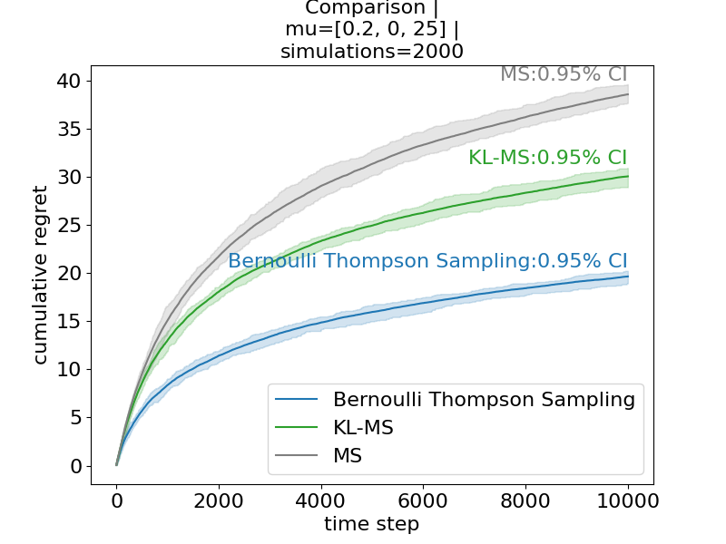
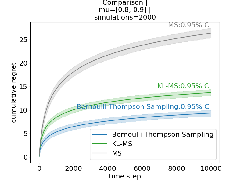
H.2 Offline evaluation

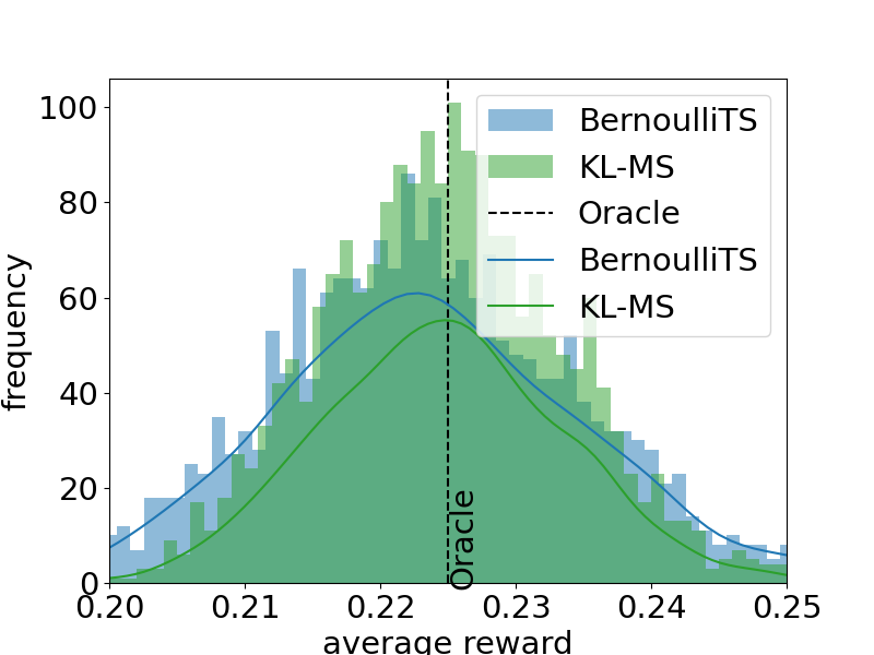
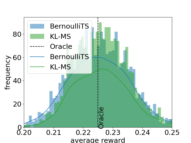
This section presents our simulation results on offline evaluation using logged data. We use the logged data generated by our algorithm, KL-MS, and standard Thompson Sampling, to estimate the expected reward of the policy that takes an action uniformly at random in $[K]$, which is equal to $\bar{\mu}=\frac{1}{K}\sum_{i=1}^{K}\mu_{i}$. The logged data are of the form $(I_{t},p_{t,I_{t}},r_{t})_{t=1}^{T}$, where $I_{t}$ is the action taken, $p_{t,I_{t}}$ is the action probability (which can be exact or approximate), $r_{t}$ is the received reward, all at time step $t$. We consider the IPW estimator [23] that estimates $\mu$, defined as

$$\hat{\mu}=\frac{1}{T}\sum_{t=1}^{T}\frac{1/K}{p_{t,I_{t}}}r_{t}.$$

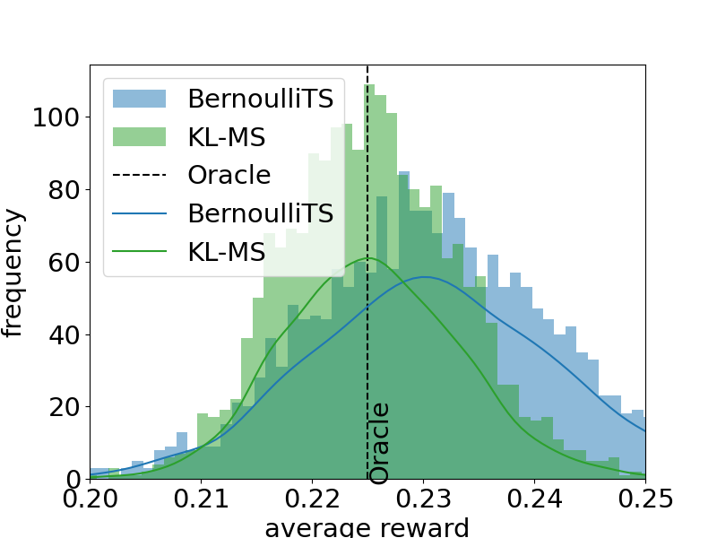
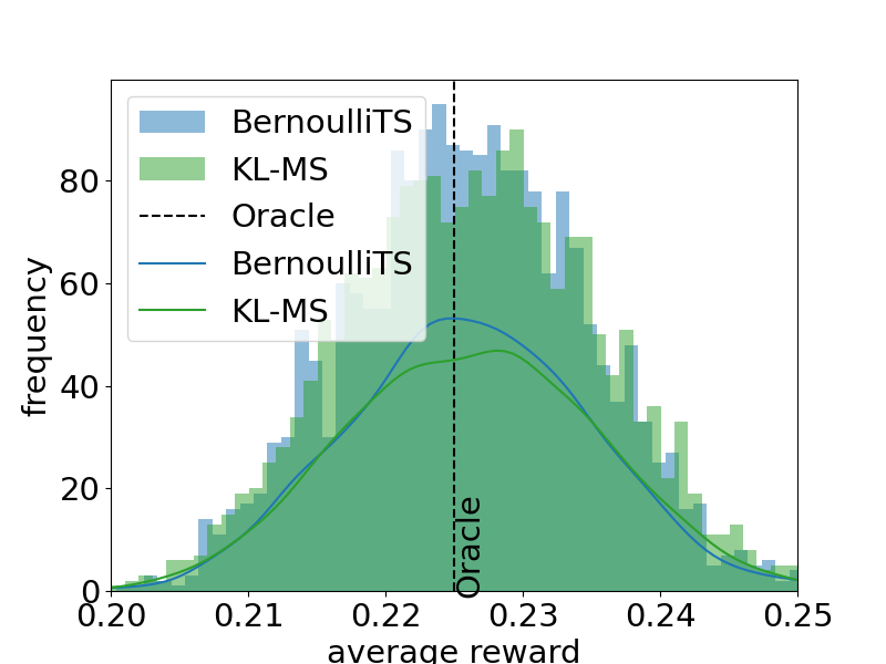
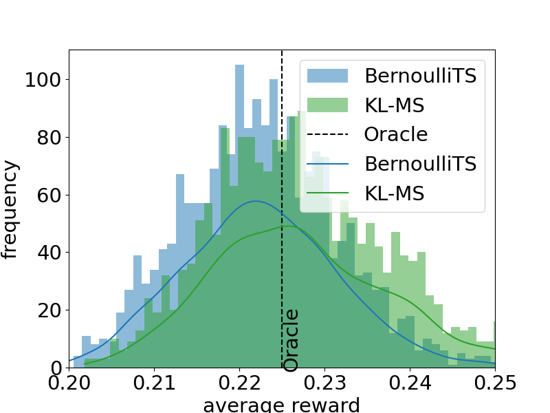
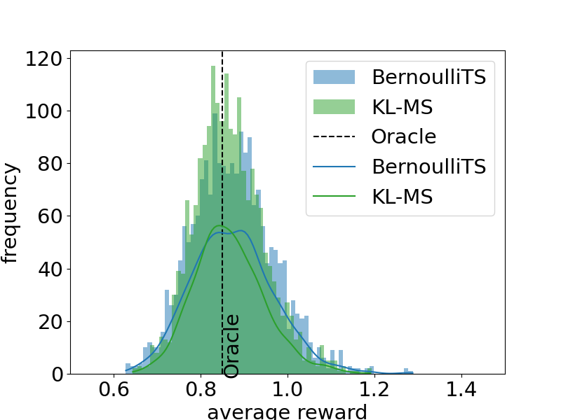
We set $T$, the time horizon of the interaction log, to be $1,000$ or $10,000$. For Thompson sampling, we use Monte Carlo (MC) to estimate the action probabilities; we vary the number of MC samples $M$ in $\mathinner{\left\{10^{3},10^{4},10^{5}\right\}}$. Note that MC estimation of action probabilities induces a high time cost: in our simulations, for $T=10^{3}$, KL-MS uses $0.43$s to generate its logged data; in contrast, BernoulliTS with $M=10^{3}$ uses $15.21$s to generate its logged data. This suggest that setting $M=10^{4}$ or $10^{5}$ may be impractical in applications.

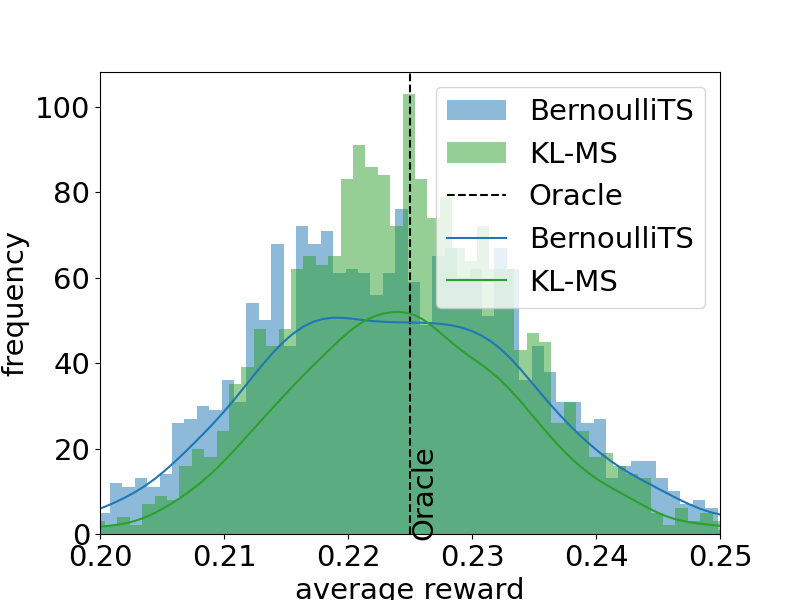
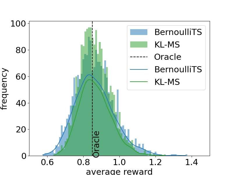
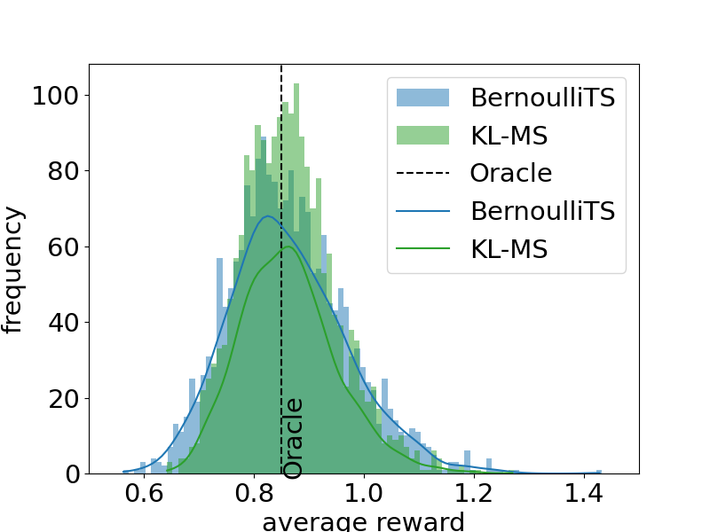
Figures 5 to 14 shows the histogram of the IPW estimates of the average reward induced by logged data generated by KL-MS and Bernoulli-TS with MC estimation of action probabilities, based on $N=2000$ independent trials in the same reward environment used in the previous experiment. Repeatedly, We have two $2$-armed bandit problems, whose mean rewards are $[0.20,0.25]$ and $[0.8,0.9]$ respectively. Tables 9 to 9 report the MSE and the bias estimate of the respective estimator. It can be seen from the figures and tables that: (1) the logged data induced by KL-MS consistently give more accurate estimates of $\mu$, compared to that of BernoulliTS with MC estimation of action probabilities; (2) the offline evaluation performance of the logged data induced by BernoulliTS is sensitive to the number of MC samples $M$; while the performance of setting $M=10^{4}$ or $10^{5}$ is on par with KL-MS, the estimation error of the more-practical $M=10^{3}$ setting is evidently higher. (3) When time step $T$ is increasing, the error between the IPW estimator induced by BernoulliTS logged data and the true performance become larger while KL-MS remains the same level of error which is smaller than the BernoulliTS.

$\mu=[0.20,0.25],T=1,000$

Figure 3: $M=10^{3}$

Figure 4: $M=10^{4}$

Figure 5: $M=10^{5}$

$\mu=[0.80,0.90],T=1,000$

Figure 6: $M=10^{3}$

Figure 7: $M=10^{4}$

Figure 8: $M=10^{5}$

$\mu=[0.20,0.25],T=10,000$

Figure 9: $M=10^{3}$

Figure 10: $M=10^{4}$

Figure 11: $M=10^{5}$

$\mu=[0.80,0.90],T=10,000$

Figure 12: $M=10^{3}$

Figure 13: $M=10^{4}$

Figure 14: $M=10^{5}$

Table 2: MSEs for $\mu=[0.20,0.25]$, $T=1,000$

	$M$
	$10^{3}$	$10^{4}$	$10^{5}$
BernoulliTS	0.00014	0.00012	0.00014
KL-MS	0.00001	0.00001	0.00001

Table 3: Bias for $\mu=[0.20,0.25]$, $T=1,000$

	$M$
	$10^{3}$	$10^{4}$	$10^{5}$
BernoulliTS	-0.00059	0.00106	-0.00068
KL-MS	-0.00096	0.00118	0.00011

Table 4: MSEs for $\mu=[0.80,0.90]$, $T=1,000$

	$M$
	$10^{3}$	$10^{4}$	$10^{5}$
BernoulliTS	0.01464	0.01143	0.01228
KL-MS	0.00733	0.00782	0.00749

Table 5: Bias for $\mu=[0.80,0.90]$, $T=1,000$

	$M$
	$10^{3}$	$10^{4}$	$10^{5}$
BernoulliTS	0.02911	0.01741	0.01636
KL-MS	0.01304	0.01412	0.01355

Table 6: MSEs for $\mu=[0.20,0.25]$, $T=10,000$

	$M$
	$10^{3}$	$10^{4}$	$10^{5}$
BernoulliTS	0.00017	0.00010	0.00009
KL-MS	0.00007	0.00006	0.00011

Table 7: Bias for $\mu=[0.20,0.25]$, $T=10,000$

	$M$
	$10^{3}$	$10^{4}$	$10^{5}$
BernoulliTS	0.00637	0.00142	-0.00240
KL-MS	0.00052	0.00066	0.00220

Table 8: MSEs for $\mu=[0.80,0.90]$, $T=10,000$

	$M$
	$10^{3}$	$10^{4}$	$10^{5}$
BernoulliTS	0.06842	0.01276	0.01220
KL-MS	0.00898	0.00804	0.00929

Table 9: Bias for $\mu=[0.80,0.90]$, $T=10,000$

	$M$
	$10^{3}$	$10^{4}$	$10^{5}$
BernoulliTS	0.17947	0.03401	0.04313
KL-MS	0.02046	0.01731	0.01123

References

- Abeille et al. [2021] M. Abeille, L. Faury, and C. Calauzenes. Instance-Wise Minimax-Optimal Algorithms for Logistic Bandits. In Proceedings of the International Conference on Artificial Intelligence and Statistics (AISTATS), pages 3691–3699, 2021.
- Agrawal and Goyal [2012] S. Agrawal and N. Goyal. Analysis of Thompson Sampling for the Multi-armed Bandit Problem. In Proceedings of the Conference on Learning Theory (COLT), volume 23, pages 39.1–39.26, 2012.
- Agrawal and Goyal [2013] S. Agrawal and N. Goyal. Further optimal regret bounds for thompson sampling. In Artificial intelligence and statistics, pages 99–107, 2013.
- Agrawal and Goyal [2017] S. Agrawal and N. Goyal. Near-optimal regret bounds for thompson sampling. Journal of the ACM (JACM), 64(5):1–24, 2017.
- Audibert et al. [2009a] J.-Y. Audibert, S. Bubeck, and Others. Minimax Policies for Adversarial and Stochastic Bandits. In Proceedings of the Conference on Learning Theory (COLT), 2009a.
- Audibert et al. [2009b] J.-Y. Audibert, S. Bubeck, et al. Minimax policies for adversarial and stochastic bandits. In COLT, volume 7, pages 1–122, 2009b.
- Audibert et al. [2009c] J.-Y. Audibert, R. Munos, and C. Szepesvári. Exploration–exploitation tradeoff using variance estimates in multi-armed bandits. Theoretical Computer Science, 410(19):1876–1902, 2009c.
- Audibert et al. [2009d] J.-Y. Audibert, R. Munos, and C. Szepesvári. Exploration–exploitation tradeoff using variance estimates in multi-armed bandits. Theoretical Computer Science, 410(19):1876–1902, 2009d.
- Auer [2002] P. Auer. Using Confidence Bounds for Exploitation-Exploration Trade-offs. Journal of Machine Learning Research, 3:397–422, 2002.
- Auer et al. [2003] P. Auer, N. Cesa-Bianchi, Y. Freund, and R. E. Schapire. The Nonstochastic Multiarmed Bandit Problem. SIAM J. Comput., 32(1):48–77, jan 2003. ISSN 0097-5397. doi: 10.1137/S0097539701398375.
- Bian and Jun [2022] J. Bian and K.-S. Jun. Maillard Sampling: Boltzmann Exploration Done Optimally. In International Conference on Artificial Intelligence and Statistics (AISTATS), pages 54–72, 2022.
- Burnetas and Katehakis [1996] A. N. Burnetas and M. N. Katehakis. Optimal adaptive policies for sequential allocation problems. Advances in Applied Mathematics, 17(2):122–142, 1996.
- Cappé et al. [2013] O. Cappé, A. Garivier, O.-A. Maillard, R. Munos, and G. Stoltz. Kullback-leibler upper confidence bounds for optimal sequential allocation. The Annals of Statistics, pages 1516–1541, 2013.
- Cesa-Bianchi et al. [2017] N. Cesa-Bianchi, C. Gentile, G. Lugosi, and G. Neu. Boltzmann exploration done right. Advances in Neural Information Processing Systems (NeurIPS), 2017.
- Chapelle and Li [2011] O. Chapelle and L. Li. An Empirical Evaluation of Thompson Sampling. In Advances in Neural Information Processing Systems (NIPS), pages 2249–2257, 2011.
- Foster et al. [2021] D. J. Foster, S. M. Kakade, J. Qian, and A. Rakhlin. The Statistical Complexity of Interactive Decision Making. CoRR, abs/2112.1, 2021.
- Garivier and Cappé [2011] A. Garivier and O. Cappé. The kl-ucb algorithm for bounded stochastic bandits and beyond. In Proceedings of the 24th annual conference on learning theory, pages 359–376. JMLR Workshop and Conference Proceedings, 2011.
- Garivier et al. [2022] A. Garivier, H. Hadiji, P. Menard, and G. Stoltz. Kl-ucb-switch: optimal regret bounds for stochastic bandits from both a distribution-dependent and a distribution-free viewpoints. The Journal of Machine Learning Research, 23(1):8049–8114, 2022.
- Harremoës [2017] P. Harremoës. Bounds on tail probabilities for negative binomial distributions. Kybernetika, pages 943–966, feb 2017. doi: 10.14736/kyb-2016-6-0943. URL https://doi.org/10.14736%2Fkyb-2016-6-0943.
- Honda and Takemura [2011] J. Honda and A. Takemura. An asymptotically optimal policy for finite support models in the multiarmed bandit problem. Machine Learning, 85(3), 2011.
- Honda and Takemura [2012] J. Honda and A. Takemura. Finite-time regret bound of a bandit algorithm for the semi-bounded support model. arXiv preprint arXiv:1202.2277, 2012.
- Honda and Takemura [2015] J. Honda and A. Takemura. Non-asymptotic analysis of a new bandit algorithm for semi-bounded rewards. J. Mach. Learn. Res., 16:3721–3756, 2015.
- Horvitz and Thompson [1952] D. G. Horvitz and D. J. Thompson. A generalization of sampling without replacement from a finite universe. Journal of the American statistical Association, 47(260):663–685, 1952.
- Jin et al. [2021] T. Jin, P. Xu, J. Shi, X. Xiao, and Q. Gu. Mots: Minimax optimal thompson sampling. In International Conference on Machine Learning, pages 5074–5083. PMLR, 2021.
- Jin et al. [2022] T. Jin, P. Xu, X. Xiao, and A. Anandkumar. Finite-time regret of thompson sampling algorithms for exponential family multi-armed bandits. In Advances in Neural Information Processing Systems, 2022.
- Kaufmann et al. [2012] E. Kaufmann, N. Korda, and R. Munos. Thompson sampling: An asymptotically optimal finite-time analysis. In Proceedings of the international conference on Algorithmic Learning Theory (ALT), pages 199–213, 2012.
- Korda et al. [2013] N. Korda, E. Kaufmann, and R. Munos. Thompson sampling for 1-dimensional exponential family bandits. Advances in neural information processing systems, 26, 2013.
- Lai et al. [1985] T. L. Lai, H. Robbins, et al. Asymptotically efficient adaptive allocation rules. Advances in applied mathematics, 6(1):4–22, 1985.
- Lattimore [2018] T. Lattimore. Refining the confidence level for optimistic bandit strategies. The Journal of Machine Learning Research, 19(1):765–796, 2018.
- Lattimore and Szepesvári [2020] T. Lattimore and C. Szepesvári. Bandit Algorithms. Cambridge University Press, 2020. URL https://tor-lattimore.com/downloads/book/book.pdf.
- Maillard [2013] O.-A. Maillard. APPRENTISSAGE SÉQUENTIEL: Bandits, Statistique et Renforcement. PhD thesis, Université des Sciences et Technologie de Lille-Lille I, 2013.
- Maillard et al. [2011] O.-A. Maillard, R. Munos, and G. Stoltz. A finite-time analysis of multi-armed bandits problems with kullback-leibler divergences. In Proceedings of the Conference On Learning Theory (COLT), pages 497–514, 2011.
- Mason et al. [2022] B. Mason, K.-S. Jun, and L. Jain. An experimental design approach for regret minimization in logistic bandits. In Proceedings of the AAAI Conference on Artificial Intelligence, volume 36, pages 7736–7743, 2022.
- Ménard and Garivier [2017] P. Ménard and A. Garivier. A minimax and asymptotically optimal algorithm for stochastic bandits. In Proceedings of the international conference on Algorithmic Learning Theory (ALT), pages 223–237, 2017.
- Ménard and Garivier [2017] P. Ménard and A. Garivier. A minimax and asymptotically optimal algorithm for stochastic bandits. In International Conference on Algorithmic Learning Theory, pages 223–237. PMLR, 2017.
- Mukherjee et al. [2018] S. Mukherjee, K. P. Naveen, N. Sudarsanam, and B. Ravindran. Efficient-ucbv: An almost optimal algorithm using variance estimates. Proceedings of the AAAI Conference on Artificial Intelligence (AAAI), 2018.
- Novak [2016] E. Novak. Some results on the complexity of numerical integration. Monte Carlo and Quasi-Monte Carlo Methods: MCQMC, Leuven, Belgium, April 2014, pages 161–183, 2016.
- Orabona [2019] F. Orabona. A modern introduction to online learning. arXiv preprint arXiv:1912.13213, 2019.
- Robins and Rotnitzky [1995] J. M. Robins and A. Rotnitzky. Semiparametric efficiency in multivariate regression models with missing data. Journal of the American Statistical Association, 90(429):122–129, 1995.
- Russo and Roy [2014] D. Russo and B. V. Roy. Learning to Optimize via Posterior Sampling. Mathematics of Operations Research, 39(4):1221–1243, 2014.
- Seldin and Slivkins [2014] Y. Seldin and A. Slivkins. One practical algorithm for both stochastic and adversarial bandits. In International Conference on Machine Learning, pages 1287–1295. PMLR, 2014.
- Thompson [1933] W. R. Thompson. On the Likelihood that One Unknown Probability Exceeds Another in View of the Evidence of Two Samples. Biometrika, 25(3/4):285, 1933.
- Wei and Luo [2018] C.-Y. Wei and H. Luo. More Adaptive Algorithms for Adversarial Bandits. In Proceedings of the Conference on Learning Theory (COLT), pages 1263–1291, 2018. URL http://arxiv.org/abs/1801.03265.
- Zimmert and Seldin [2021] J. Zimmert and Y. Seldin. Tsallis-inf: An optimal algorithm for stochastic and adversarial bandits. The Journal of Machine Learning Research, 22(1):1310–1358, 2021.