Interpreting Vision and Language Generative Models with Semantic Visual Priors
Abstract
When applied to Image-to-text models, interpretability methods often provide token-by-token explanations namely, they compute a visual explanation for each token of the generated sequence. Those explanations are expensive to compute and unable to comprehensively explain the model’s output. Therefore, these models often require some sort of approximation that eventually leads to misleading explanations.
We develop a framework based on SHAP, that allows for generating comprehensive, meaningful explanations leveraging the meaning representation of the output sequence as a whole. Moreover, by exploiting semantic priors in the visual backbone, we extract an arbitrary number of features that allows the efficient computation of Shapley values on large-scale models, generating at the same time highly meaningful visual explanations.
We demonstrate that our method generates semantically more expressive explanations than traditional methods at a lower compute cost and that it can be generalized over other explainability methods.
\helveticabold1 Keywords:
vision and language, multimodality, explainability, image captioning, visual question answering, natural language generation
2 Introduction
Multimodal learning research has witnessed a surge of effort leading to substantial improvements, in algorithms involving the integration of vision and language (V&L ), for tasks such as image captioning (Lin et al., 2014; Hossain et al., 2019; Sharma et al., 2020) and visual question answering (Antol et al., 2015; Zhu et al., 2016; Srivastava et al., 2021). The need has arisen to create more challenging tasks and benchmarks requiring higher fine-grained linguistic capabilities (Parcalabescu et al., 2022; Thrush et al., 2022) and semantic and temporal understanding (Yu et al., 2016; Park et al., 2020).
In this context, the role of interpretability methods has become central to assessing the models’ grounding capabilities. However, such tools are often designed for specific classes of tasks or models. To overcome this limitation, model-agnostic interpretability methods, such as SHAP-based methods (Lundberg and Lee, 2017), are often preferred over others, since they rely on a solid theory and benefit from desirable properties not available in other methods.
When such methods are applied to V&L generative tasks, like image-captioning, the goal is to explain the textual output with reference to the visual input. However, the text generation process happens token-by-token, and as a result, most of the interpretability methods applied in this context tend to produce local token-by-token explanations. Moreover, for most applications, current methods build the explanation on top of arbitrary regions of the visual input.
Such explanations are hard to interpret as they are token-specific, and they are costly to compute since the number of models’ evaluations grows exponentially with the number of features used in each explanation. To mitigate these issues, approximation techniques, like sampling, and input feature reduction are usually applied. However, this produces inaccurate explanations which lack detail and are hard to interpret.
In this work, we address these issues by proposing:
-
1.
a modular framework to create a new family of tools to generate explanations in V&L generative settings;
-
2.
a method to generate sentence-based explanations for vision-to-text generative tasks, as opposed to token-by-token explanations, showing that such explanations can efficiently be generated with SHAP by exploiting semantic knowledge from the two modalities;
-
3.
a method to reduce the number of visual input features by exploiting the semantics embedded in the models’ visual backbone. We extend this method to a number of different architectures, performing a systematic comparative study and we propose an alternative for the architectures not suitable for this method;
-
4.
a human evaluation designed to assess key user-centric properties of our explanations.
3 Related Work
3.1 Interpretable Machine Learning
Interpretable machine learning is a multidisciplinary field encompassing efforts from computer science, human-computer interaction, and social science, aiming to design user-oriented and human-friendly explanations for machine learning models. It plays an important role in the field for a series of reasons: it increases trust, confidence, and acceptance of machine learning models by users, and enables verification, validation, and debugging of machine learning models. Techniques for deep neural networks (DNN) can be grouped into two main categories: white-box methods which exploit the knowledge of the internal structure of the model to generate the explanation and black-box methods, also called model-agnostic, which operate only on the inputs and the outputs (Loyola-Gonzalez, 2019).
White-box methods. There exist two types of white-box methods: attention-based and gradient-based methods. Attention-based methods (e.g. Ahmed et al., 2021; Zheng et al., 2022) exploit the model’s attention activations to identify the part of the input attended by the model during the prediction. They can be used to explain predictions in diverse tasks, like image recognition (Li et al., 2021), authorship verification (Boenninghoff et al., 2019) gender bias identification (Boenninghoff et al., 2019) etc. On the other hand, Gradient-based methods (Springenberg et al., 2014; Selvaraju et al., 2017) compute feature attributions by manipulating the gradients computed in the backward step with respect to the original inputs (Shrikumar et al., 2016), or with respect to a specific baseline (Sundararajan et al., 2017; Simonyan et al., 2013).
Black-box methods do not make any assumptions regarding the underlying model. For example, Permutation Feature Importance (Breiman, 2001), initially designed for random forests and later extended into a model-agnostic version by Fisher et al. (2019), consists in randomly shuffling the input features and evaluating the model’s output variations. Ribeiro et al. (2016) proposed LIME for Local Interpretable Model-Agnostic Explanation. This method uses a surrogate linear model to approximate the black-box model locally, that is, in the neighborhood of any prediction. LOCO (Lei et al., 2018) is another popular technique for generating local explanation models. It can provide insight into the importance of individual variables in explaining a specific prediction. SHAP (Lundberg and Lee, 2017) is a framework considered by many to be the gold standard for local explanations, thanks to its solid theoretical background. SHAP leverages the concept of Shapley values, first introduced by (Shapley et al., 1953), used to measure the contribution of players in a cooperative game. This was later extended by (Lundberg and Lee, 2017) for the purpose of explaining a machine learning model.
In this work, we propose a flexible hybrid framework based on SHAP, which benefits from properties typical of black-box methods, since it can be applied in a completely model-agnostic way. At the same time, our method shares some properties with white-box approaches since, when possible, it takes advantage of certain internal components of the model. In particular, the framework we propose for Vision-Language generative models can be leveraged to exploit architectural features of a model’s visual backbone to generate more semantically meaningful explanations.
3.2 Background on SHAP
In the context of machine learning, the cooperative framework introduced by Shapley et al. (1953) can be framed as a game where each input feature is a player and the outcome is determined by the model’s prediction. Shapley values measure the contribution of each player to the final outcome, or in other words, the input features’ importance. Shapley redistributed the total outcome value among all the features, based on their marginal contribution across the possible coalitions of players, i.e. combinations of input features. The outcome of the game, namely the prediction of the model, is redistributed across the features, in the form of contributions that have three desirable properties:
-
•
Efficiency: all the Shapley values add to the final outcome of the game;
-
•
Symmetry: all the features generating the same outcome in the game have the same Shapley value, thus the same contribution;
-
•
Dummy: if adding a feature to a coalition (i.e. set of features) does not change the outcome of the game, its Shapley value is zero.
Furthermore, Lundberg and Lee (2017) contribute by formulating a variety of methods to efficiently approximate Shapley values in different conditions:
-
1.
KernelSHAP: derived from LIME and totally model agnostic, hence the slowest within the framework;
-
2.
LinearSHAP: designed specifically for Linear models;
-
3.
DeepSHAP: adapted from DeepLift (Shrikumar et al., 2017) for neural networks, which is faster than KernelSHAP, but makes assumptions about the model’s compositional nature.
Later on, the framework was extended with other methods with variations for specific settings; Mosca et al. (2022a) propose a thorough description of the SHAP family of methods.
It is important to note that all these methods work under the so-called feature independence assumption, which is fundamental for the theoretical resolution of the problem. However, in order to deal with real-life scenarios, this constraint is relaxed to some extent. For instance, in Natural Language Processing tasks each token of a textual sequence is considered an independent feature (Kokalj et al., 2021) whereas, in Computer Vision, the image is usually split into squared patches also considered independent of each other (Jeyakumar et al., 2020). In both of these cases, the independence assumption is a simplification. For example, language tokens are often mutually dependent in context (and this is indeed the property leveraged by self-attention in Transformer language models). Similarly, pixels in neighboring patches in an image may well belong to the same semantically relevant region (and this is indeed the property exploited by neural many architectures suited for computer vision tasks, such as convolutional networks). Properties of tokens in context and those of pixels in image regions, have been taken into account in some adaptations of SHAP which consider the hierarchical structure of the feature space, such as HEDGE for text (Chen et al., 2020) and h-SHAP for images (Teneggi et al., 2022).
Our framework relies on KernelSHAP as is it totally model-agnostic. We address both the efficiency issue and the strict independence assumption of the method by generating semantic input features (more details in Section 4.3) and optimizing the approximation through sampling (full details in Section 4.1.1).
3.3 Explainability for Vision and Language
One way to characterize the scope of V&L models is with respect to the types of tasks they are designed to address. On the one hand, tasks like image captioning (Fisch et al., 2020; Zhang et al., 2021; Anderson et al., 2018; Mokady et al., 2021; Li et al., 2022a), image-text retrieval (Cao et al., 2022; Radford et al., 2021), and visual question answering (Antol et al., 2015) require a strong focus on the recognition of objects in images. More recently, research has begun to explore the capabilities of models in tasks that require some further reasoning or inference over the image contexts, such as understanding analogies (Zhang et al., 2019a), describing actions and rationales (Cafagna et al., 2023) and inferring temporal relations (Park et al., 2020).
The need to understand how V&L models ground their predictions has become essential, leading to the emergence of Explainable Artificial Intelligence (XAI) for multimodal settings (Zellers et al., 2019). Visual explanations can help humans to know what triggered the system’s output and how the system attended to the image. To this purpose, feature attribution methods are often preferred as they can provide a visual explanation of the prediction. Most of the XAI methods introduced for unimodal tasks can be adapted to V&L tasks.
Some popular white-box methods use gradients to generate saliency maps to highlight the pixels corresponding to highly contributing regions. These methods include Grad-CAM (Selvaraju et al., 2017; Shrikumar et al., 2016) or Layer-wise Relevance Propagation (LRP) (Binder et al., 2016) where the contribution is computed with respect to an intermediate layer instead of the input layer. These methods can produce fine-grained pixel-level explanations. However, their outcomes can be noisy and require many evaluations to converge to a stable explanation.
Black-box approaches are mostly perturbation-based, that is, they compute attributions based on the difference observed in the model’s prediction by altering the input. Such methods include occlusion sensitivity, RISE (Petsiuk et al., 2018), and LIME (Ribeiro et al., 2016). Other approaches are task-agnostic, like MM-SHAP (Parcalabescu and Frank, 2022), where a SHAP-based method is used to measure the contribution of the two modalities in V&L models independently of the task performance. Although these methods make few assumptions about the underlying model, their explanations are computationally expensive, as the number of model evaluations required grows exponentially with the number of features. To overcome this limitation, the number of features is usually reduced by partitioning the image into patches called superpixels, which discretize the input into a smaller number of features. However, this approach can lead to coarser and not very informative explanations.
3.3.1 Generative tasks
Explanations for V&L generative tasks like image captioning incur even more complexity, as the prediction of the model is now a textual sequence. A popular solution, which is in keeping with the autoregressive nature of neural language decoders, is to break down the caption generation process into a series of steps where each token is explained separately with respect to the image and the previously generated sequence. This requires generating a single visual explanation for each generation step. However, the meaning of the sentence is not only determined by the meaning of the single words it is composed of, but also by the way these words are combined and arranged together. Therefore, a global meaningful explanation must take into account the whole textual sequence and not just part of it, as only in this way can the explanation take into account the whole textual context.
A popular solution is to generate the token-level explanations using Integrated Gradients (Sundararajan et al., 2017), providing region-level visualizations or using the attention activation scores to visualize the model’s attended regions (Cornia et al., 2022; Zhang et al., 2019b). However, these methods are white-box approaches as they make assumptions about the inner workings of the model, thus they need to be specifically re-adapted to new systems. Furthermore, they focus on token-level explanations but do not allow a comprehensive global explanation of the textual output.
To the best of our knowledge, our work is the first attempt to bring together a model-agnostic framework like SHAP, in the image-to-text task, with the aim of providing a comprehensive explanation of the generated textual output as a whole, rather than on a token-by-token level.
4 Method
4.1 Kernel Shap
The core method of our framework is Kernel Shap. We base our approach on the formulation by Lundberg and Lee (2017), which provides an accurate regression-based, model-agnostic estimation of Shapley values. The computation is performed by estimating the parameters of an explanation model which matches the original model , namely:
| (1) |
where is the number of input features (or players) and is a player of the game. is approximated by performing a weighted linear regression using the Shapley kernel:
| (2) |
where is the subset of non-zero entries, namely a binary representation of the coalition of players. The Shapley kernel, in other words, is a function assigning a weight to each coalition. The number of coalitions needed to approximate the Shapley values corresponds to all the possible combinations of players, i.e. coalitions. This makes Kernel SHAP extremely expensive to compute (and slow in practice) when is large.

4.1.1 Kernel SHAP Sampling
Kernel SHAP is model-agnostic, meaning that it cannot make any assumption on the model to explain. For this reason, it is also among the slowest in the SHAP family of XAI methods (Mosca et al., 2022b). This issue is addressed by performing Monte Carlo sampling over the pool of coalitions, allowing under certain conditions to compute a reasonably accurate approximation of the Shapley values, even in the case of large-sized models or low-resource hardware.
Taking inspiration from Molnar (2020), we implement a deterministic sampling strategy, where we prioritize the high-weight coalitions, whose weight is computed by Eq. 2, when applying a certain sampling budget. This is achieved by generating the coalitions in decreasing weight order and selecting the first coalitions, where corresponds to the sampling budget. In Figure 1 we compare the plots of the coalition’s weights computed using the standard Kernel SHAP (on the left) and prioritizing high-weight coalitions (on the right); as observed, our sampling strategy with priority (on the right) ensures selecting the high-weight coalitions first, providing an optimal ordering among samples.
Sampling with priority offers two main advantages:
-
1.
higher accuracy of the Shapley values estimate;
-
2.
a deterministic sampling strategy.
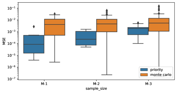
In Figure 2 we report the approximation error of the Shapley values when applying Kernel SHAP, using Monte Carlo (orange) and the high-weight priority (blue) as sampling strategy, for different sampling sizes. The error is computed over runs, using the Mean Squared Error (MSE) with respect to the Shapley values computed with Kernel SHAP using all the coalitions. Our sampling with priority approximates Shapley values with errors that are orders of magnitude smaller than Monte Carlo sampling, consistently, for different sampling sizes.
4.1.2 How to adapt Kernel SHAP to Vision and Language Generative Tasks
In the image captioning scenario, we can set up a cooperative game, where we want to compute the contributions of the players, i.e. the pixels of the image, with respect to the outcome, i.e. the caption. In this section, we identify two shortcomings of the standard way in which this is performed and discuss our contributions to overcome these shortcomings, which were pointed out in Section 3 above.
The first problem is related to the definition of coalitions in the visual input. The number of coalitions to be computed grows exponentially with the number of players. This makes the computation of the Shapley values intractable for images and makes any sampling strategy completely inaccurate. In order to overcome this limitation, the image is typically partitioned into a grid composed of superpixels, namely groups of pixels, each of which represents a single player. This reduces the total number of players in the game, making computation of the Shapley values more feasible, but at the same time, it reduces the degree of the detail of the explanation. Moreover, we argue that breaking the image into a grid of square superpixels breaks the semantics underlying the image, resulting in potentially under-informative explanations. In particular, there is no guarantee that the pixels grouped together in this manner correspond to semantically meaningful image regions.
The second problem is related to the comprehensiveness of explanations. In order to measure the variations of the outcome of the function needed to run Kernel SHAP, the caption generation process is usually broken down into token generation steps. Each step produces logits that can be used to compute a numerical outcome. However, this forces us to consider each generation step as a separate cooperative game, meaning that we need to run a separate instance of Kernel SHAP for each generated token, further increasing the time and compute cost needed to explain an image-caption pair. Moreover, such explanations refer to single tokens and do not provide an explanation for the whole output of the model, namely the caption.
4.2 Towards Sentence-based explanations
As explained in Section 4.1, Shapley values are computed with respect to a numerical value representing the outcome of the function we are interested in explaining. With generative models, this is typically done on a token-by-token basis. For example, in an image captioning scenario, this is achieved by measuring variations in the logit of the generated tokens for the caption, at each time step. Such token-based explanations are useful to assess the grounding of a specific part of speech - like nouns and verbs - but fail in providing a global explanation that takes into account the meaning of the whole sentence.
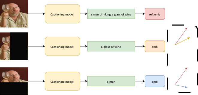
On the other hand, with a whole caption, we lack the numerical output against which to compute the attributions. In order to adapt Kernel SHAP to generate global explanations for the caption, we measure variations of the caption meaning representation when perturbations are applied to the image in input. This allows us to numerically quantify the meaning variation of the whole caption. Formally, given an image-captioning model and an image we generate a caption and we compute:
| (3) |
where is the embedding representation of that we consider the reference embedding of the caption, and is a function used to extract such a representation.
For each perturbed image and its corresponding caption we extract, analogously, an embedding , then we compute:
| (4) |
where is the variation in the embedding representation computed as the cosine distance , between the reference embedding and the embedding of the caption of the perturbed image .
In other words, we use the cosine distance between the semantic representation of the reference caption and the caption generated upon input perturbation, to measure the model’s variations; a schematic representation of the method is shown in Figure 3. Re-framing the problem as described allows us to apply Kernel SHAP to compute feature attributions taking into account the semantic variation of the whole caption in a single cooperative game instance.
4.3 Exploiting Semantic Visual Priors
Partitioning the image into a grid of superpixels is a straightforward way to reduce the number of input features in the image. We argue that, although convenient, superpixels do not guarantee the preservation of semantic information depicting the visual content, as they shatter the image into equally sized patches regardless of the content represented. We address this issue by proposing a semantically guided approach, that selects the input features according to semantics-preserving visual concepts arising from the visual backbone of the V&L model. This not only allows for generating more meaningful explanations but explicitly focuses explanations of the model’s generative choices on the output of the model’s own visual backbone.
We generate input features leveraging the Deep Feature Factorization (DFF) method (Collins et al., 2018). DFF is an unsupervised method allowing concept discovery from the feature space of CNN-based models. We refer to such concepts as ‘semantic priors’, that is, the knowledge or assumptions learned by the visual backbone, for a given domain or task. We use them to craft input features that produce semantically informed visual explanations.
Formally, following Collins et al. (2018)’s notation, given the activation tensor for an image :
| (5) |
where correspond respectively to the height and width, and the number of channels of the visual backbone’s last activation layer, we perform a non-negative matrix factorization (NMF) of :
| (6) |
where and enforce the dimensionality reduction to rank .
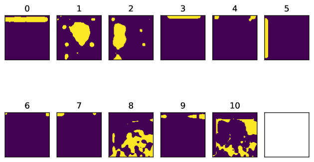
Each column can be reshaped into heatmaps of dimensions , each of which highlights a region that the factor corresponds to. The heatmaps are then upsampled to match the original image size with bilinear interpolation and converted to binary masks, each of which corresponds to an input feature. In this way we obtain input features, where is the number of concepts extracted. A schematic example of input feature extraction performed by DFF is shown in Figure 4.
In our method, the regions identified via DFF are the features for which attributions are computed. The key intuition is that these features correspond to meaningful sub-parts of the input image according to the V&L model’s visual backbone. They do not necessarily reflect humans’ visual expectations of the image; rather they represent the visual priors learned by the vision model after training.
To create a coalition we sum up multiple masks, then apply them to the original image which will contain only pixels belonging to input features in the selected coalition.
NMF can be seen as an unsupervised clustering algorithm, allowing control for the number of clusters or concepts to find. can be considered a hyperparameter of the method, which we show can be kept small to achieve a good level of semantic detail and low compute cost.

4.3.1 Non-partitioning features
DFF generates semantic masks reflecting the activations of the model’s visual backbone. The whole process is unsupervised and produces masks that do not constitute partitions of the image, meaning that it is not guaranteed that the sum of all the extracted masks will match the total size of the image. In order to account for this issue, we create an additional leftover mask covering the remaining area and we include it in the SHAP cooperative game, this allows us to consider the whole visual information represented by the image, in the game.
4.3.2 Intensity-preserving explanations
SHAP-based methods relying on superpixels assume that each pixel in a patch contributes equally, thus all the pixels in a patch are assigned the same Shapley value. However, in DFF, features in each binary mask correspond to an equally sized heatmap. Therefore, we multiply the Shapley value by the heatmap corresponding to the binary mask. This allows scaling the contribution according to the intensity of the feature signal.
5 Experiments
The methodology described in the previous section raises two questions which we now address experimentally:
-
1.
What are the pros and cons of our method based on visual semantic priors in comparison with standard feature selection methods used in V&L , based on superpixels?
-
2.
What are the benefits and potential limits of our method for human users, in terms of relevant dimensions such as intensity, detail, efficiency, and flexibility?
5.1 Data
We validate the method presented in the previous section with experiments using the HL image caption dataset. The HL dataset (Cafagna et al., 2023) contains 15k images extracted from COCO (Lin et al., 2014). The dataset pairs images with captions that describe the visual contents along three different high-level dimensions, namely scenes, actions and rationales for the actions. These are additionally paired with the original COCO captions, which provide a more low-level, object-centric description. The annotations were collected by asking annotators three questions related to each of the three high-level dimensions. The systematic alignment of the object-centric and abstract captions provides us with a suitable test bed to compare the efficacy of our method in delivering global explanations in both captioning and visual question-answering scenarios. An example pairing the three high-level captions and the original COCO caption from the HL Dataset is shown in Table 1.
| Image | Axis | Caption |
|---|---|---|
![[Uncaptioned image]](/html/2304.14986/assets/img/hl_example_6780.jpg)
|
scene | at a sport field |
| action | they are playing a sport | |
| rationale | they are having fun | |
| object-centric (COCO) | A woman has fallen on the ground in a field. |
5.2 Model
For our experiments, we focus on one V&L model, since our goal is to evaluate the quality of explanations. Our choice is motivated by two considerations: first, a model should ideally have good performance in zero-shot settings; second, it should exhibit state-of-the-art performance on generative tasks. OFA (Wang et al., 2022) is a large pre-trained multimodal model trained using a task-agnostic and modality-agnostic framework. OFA is able to perform a diverse set of cross-modal and unimodal tasks, like image captioning, visual question answering, image generation, image classification, etc. OFA is trained on a relatively small amount of data (20M image-text pairs) with instruction-based learning and a simple sequence-to-sequence architecture. Nevertheless, on downstream tasks, it outperforms or is on par with larger models trained on a larger amount of data. OFA is effectively able to transfer to unseen tasks and domains in zero-shot settings, proving to be well grounded also in out-of-domain tasks.
This makes OFA an excellent candidate to test our explainability framework in a real-world scenario, namely a large pre-trained generative model with SOTA performance on downstream tasks in zero-shot conditions.
5.3 DFF vs Superpixel
In this Section, we focus on the comparison between the global visual explanations produced using superpixel or DFF input features. We focus on the capability of the two methods to adapt to different semantic aspects of the explanation; in Section5.3.1 we specifically address this discussion leveraging the VQA task.
All the experiments are performed in zero-shot by using OFA-large model in its original implementation 111https://github.com/OFA-Sys/OFA. In order to ensure a fair comparison, we extract a similar number of features for both methods, namely for superpixel and for DFF. This number allows us to execute the experiments in a reasonable amount of time. In fact, we recall that the number of features has an exponential impact on the number of model evaluations needed to generate the explanations. Reducing the number of features mitigates the efficiency issue, but does not solve it. An in-depth discussion about the efficiency issue is provided in Section 5.3.2.
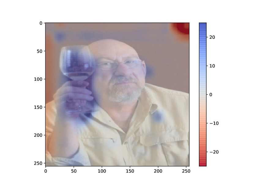
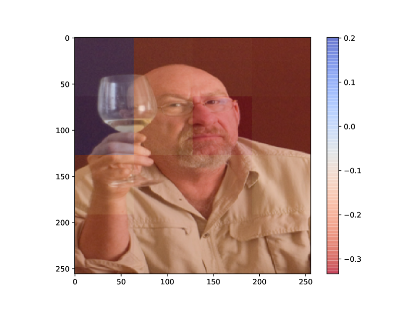
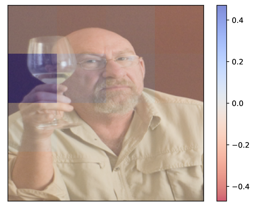
As an initial comparison, Figure 5 shows a direct comparison between the two kinds of input features for the caption ”drinking”, generated using sentence-based Kernel SHAP. Both methods assign a positive contribution to the region corresponding to the glass, with some important differences:
-
•
Detail: The DFF features succeed in capturing the key visual semantics of the image, i.e. the glass, in a single input feature (with some noise), producing a more detailed explanation than superpixel, where the region corresponding to the glass is shared across different patches (i.e. different features).
-
•
Intensity: DFF scales the contributions according to the magnitude of the feature signal (as described in Section 4.3.2), providing additional information regarding the importance of a specific area within the same input feature region.
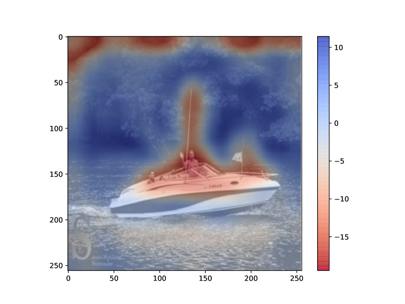
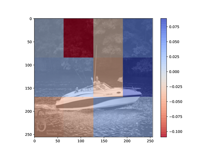
Q: What is the subject doing? A: boating
Q: Where is the picture taken? A: lake
Q: What is the subject doing? A: eating
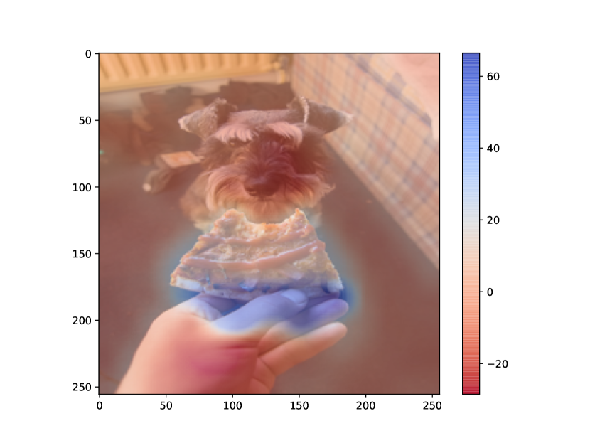
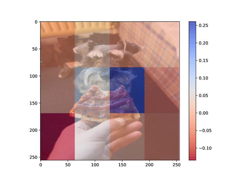
Q: Where is the picture taken? A: in a living room
5.3.1 Semantic visual features improve the quality of the explanations
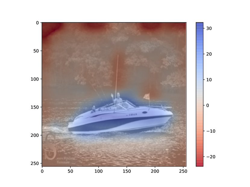
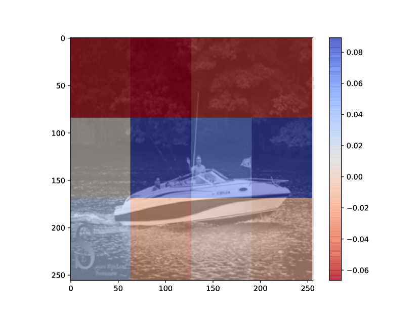
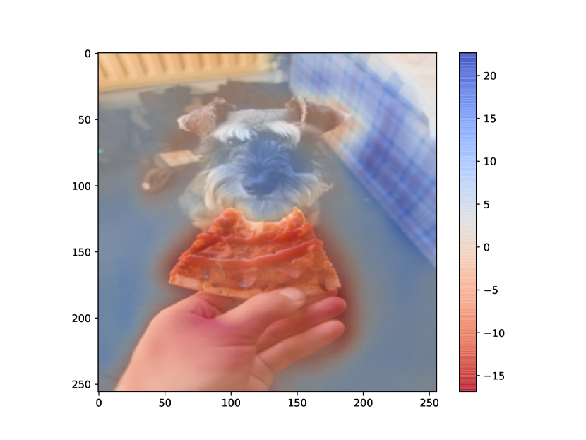
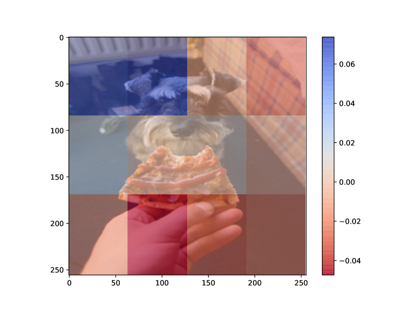
We compare DFF and superpixel explanations on the VQA task. We select images and questions for the three axes in the HL dataset, i.e. action, scenes, and rationales, and we generate visual explanations for the answers. This allows us to compare how the two methods handle semantically different aspects highlighted in the visual content.
We expect to see that the positive contribution assignment (in blue) changes for the same image for different captions, corresponding to different kinds of questions. In response to different questions about location, rationale, or action, the model’s output should depend on different regions of the image. For instance, we expect to observe a wider positive area highlighted in the picture for the where question and a more specific detailed area for the what question. As shown in Figure 6, the DFF-based method (middle row) succeeds in highlighting in significant detail the semantic areas contributing to the output. On the other hand, superpixels provide coarser detail, as it is limited by the size of the patches. This suggests that the DFF-generated explanations could lead to a visible advantage in terms of comprehensiveness and completeness; we further test these hypotheses by running a human evaluation, in Section 6.
5.3.2 Semantics-guided explanations are efficient
In order for superpixel-based explanations to achieve a level of detail comparable to DFF, we need to significantly increase the number of patches. However, this causes an exponential surge in computing cost, which makes it unfeasible to run, especially if we are testing large models. This issue can be mitigated by performing Kernel SHAP sampling (as described in Section 4.1.1). The combination of the exponential growth of the sample space, and the limited sampling budget can easily lead to unreliable explanations. An example is shown in Figure 5.3.2 where we perform Kernel SHAP sampling with a budget of samples, which is the same budget used to compute the DFF explanation in Figure 5.
On the other hand, DFF does not suffer from this issue. In fact, there is no clear advantage in increasing the number of features, because the main semantic content is already embedded in a small number of features. In our experiments, we establish that a good number of features for DFF is between and . This number of features keeps the computational cost low, allowing to compute full Kernel SHAP or Kernel SHAP sampling with very high accuracy. We provide full details in the supplemental material.
minipage0.32
![[Uncaptioned image]](/html/2304.14986/assets/x16.png)
8X8
![[Uncaptioned image]](/html/2304.14986/assets/x17.png)
16X16
5.4 Semantic Features Analysis
The semantic features extracted by DFF are drastically different from superpixel features in many key aspects related to the visual content captured. Moreover, DFF is unsupervised and dynamically exploits the visual backbone’s priors. In this Section, we focus on analyzing the benefits and limitations characterizing the semantic features generated by DFF. We discuss in detail key aspects like the kind of semantic content captured along with possible theoretical implications and how it can be generalized over different visual backbones.
5.4.1 What kind of semantics do DFF features capture?
DFF features capture semantic concepts learned by the model’s visual backbone. These do not necessarily follow human visual expectations. In Figure 7 we show an example: features 1, 2, and 8 can be associated with three main semantic objects and entities of the image, namely face, glass and shirt. However, we observe in the remaining features several geometrical patterns, that highlight the edges and the corners of the pictures. This pattern is recurrent in the features extracted by DFF, independently of the visual content. We believe this is partially due to the capability of CNNs to capture spatial configuration (Zeiler and Fergus, 2014) and the effectiveness of DFF, in factorizing together model activations with similar characteristics.
5.4.2 Relaxing the feature independence assumption
As described in Section 3.2, SHAP in the cooperative game formulation assumes the feature independence principle, namely that each feature is independent of all the others. However, this assumption does not hold for image data since each pixel is inherently dependent on the other pixels, especially those in its vicinity, in representing the visual content. Therefore, in order to work with visual data, this constraint needs to be relaxed. This solution is typically applied for computer vision tasks by graphical models like Conditional Random Fields (CRF). CRFs relax the strong dependence assumption on the observations (the pixels of the image) by modeling the joint distribution of observations, usually intractable, as a conditional distribution (Li et al., 2022b).
![[Uncaptioned image]](/html/2304.14986/assets/x19.png) Non-disjoint features
Non-disjoint features
![[Uncaptioned image]](/html/2304.14986/assets/x20.png) Disjoint features
Example of overlap (highlighted in red) between two feature masks (Figure 5.4.2) and comparison between visual explanations generated given the question ”What is the subject doing?” and the model’s answer ”drinking”, with regular DFF features (Figure 5.4.2) and disjoint DFF features (Figure 5.4.2). Although the masks overlap only to a small extent, the explanation is visibly affected.
Along the same lines, superpixel features relax this constraint by partitioning the image into patches that are not independent, considering the underlying semantics depicted in the visual content.
This issue is mitigated by the DFF features, as they tend to cover semantically related regions of the image, preserving the underlying visual semantics. On the other hand, as pointed out in Section 4.3.1, DFF features are not disjoint, meaning that to some extent, the contribution of overlapping regions is subject to contamination from other regions. In this section, we analyse the consequences of this in more detail. Our analysis follows two steps:
Disjoint features
Example of overlap (highlighted in red) between two feature masks (Figure 5.4.2) and comparison between visual explanations generated given the question ”What is the subject doing?” and the model’s answer ”drinking”, with regular DFF features (Figure 5.4.2) and disjoint DFF features (Figure 5.4.2). Although the masks overlap only to a small extent, the explanation is visibly affected.
Along the same lines, superpixel features relax this constraint by partitioning the image into patches that are not independent, considering the underlying semantics depicted in the visual content.
This issue is mitigated by the DFF features, as they tend to cover semantically related regions of the image, preserving the underlying visual semantics. On the other hand, as pointed out in Section 4.3.1, DFF features are not disjoint, meaning that to some extent, the contribution of overlapping regions is subject to contamination from other regions. In this section, we analyse the consequences of this in more detail. Our analysis follows two steps:
-
1.
We measure the DFF feature overlap over a sample of 1000 images. We find that the amount of overlap among the feature masks corresponds to the of the pixels in the image with a standard deviation of and an average maximum peak of . This suggests that this phenomenon is present to a limited extent.
-
2.
We compare visual explanations generated by disjoint and non-disjoint features. In order to generate disjoint features, we post-process the feature masks extracted, by checking all possible pairs of feature masks and assigning the possible overlapping region to one of the two compared features. An example is shown in Figure 5.4.2 where the overlapping regions (highlighted in red) between two feature masks are randomly assigned to one of the features (either blue or green).
Enforcing the features’ disjointness leads to similar results to their non-disjoint counterpart. However, in some cases, the re-allocation of the overlapped region impacts the Shapley value of the feature, causing unpredictable results. This suggests that manually changing the feature masks can disruptively affect the visual semantics captured by the feature, leading to misleading visual explanations. A cherry-picked example is shown in Figure 5.4.2, where using the disjoint features (Figure 5.4.2) causes a meaningful change in the visual explanation. In conclusion, we observed that the phenomenon of the non-disjoint features is present to a small extent and overall it does not invalidate the visual explanations as it can be considered a relaxation of the feature independence assumption. Moreover, as empirically observed, relaxing this assumption is unlikely to invalidate the method, as the explanation is consistent with the ones generated by superpixel features. On the other hand, we observed that forcing the feature masks’ disjointness harms their capability to preserve the visual semantics, leading to misleading visual explanations.
minipage0.32
5.4.3 Does the feature size matter?

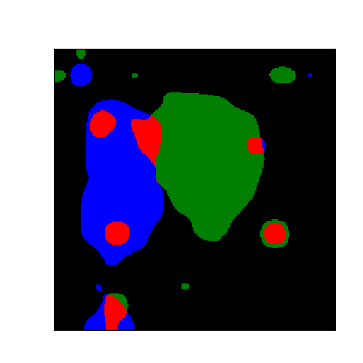
Differently from superpixel patches, DFF semantic features can have different sizes, depending on the semantic role of the highlighted region. We ask to what extent the size of a visual feature could affect the final contribution in the SHAP cooperative game. In order to test for that, we normalize the Shapley value obtained according to the size of the feature mask and we compare normalised values with the unnormalized ones. To normalize a Shapley value we compute:
| (7a) | |||
| (7b) | |||
where is a non-zero element of the binary mask, is the total number of entries in mask and indicates the proportion of the image covered by the mask. is then used to discount the magnitude of the Shapley value obtaining the normalized value . In the normalization process, the feature contribution’s magnitude is obviously re-scaled. However, we are interested in measuring to what extent the normalization has affected the features’ importance in relative terms. Therefore, we use the Rank Biased Overlap (RBO) (Webber et al., 2010), a similarity metric for ranked lists, to measure the difference in the feature attribution ranking after normalization for a sample of 100 DFF-based explanations. A significant change in feature ranking would entail a positive correlation between size and feature importance. In Figure 8 we show the results of this experiment: the RBO is overall at the ceiling, with a minimum value of (in a range where is identical ranking and is totally different). The positive contributions, which are the most informative to understand the explanations, are the most stable in terms of ranking. This suggests that the size of the features extracted using DFF, does not significantly affect the final contribution of the semantic feature and does not harm the visual explanations.
5.5 Does DFF adapt to other visual backbones?
DFF is designed to perform concept discovery in CNN-based visual backbones. However, current pre-trained V&L models’ vision encoder often rely on different architectures, such as Vision Transformers (ViT) (Dosovitskiy et al., 2020), FasterRCNNs (FRCNN) (Ren et al., 2015), or their variants. In this section, we show how DFF can be adapted to these architectures. Moreover, we provide an alternative solution to perform model-agnostic semantic feature extraction, which is applicable to any architecture.

5.5.1 Vision Transformers
In order to apply DFF to ViT encodings, we need to take into account two substantial differences with respect to CNNs: (1) firstly, ViT splits the image into a grid of patches and generates an embedding vector for each patch. To obtain an activation matrix, each embedding vector is stacked together and a special vector is added in position to indicate the beginning of the sequence. Differently from the CNNs, the spatial information related to the patch is lost in the encoding process and added later on, by concatenating a positional embedding to the embedding vectors. (2) Secondly, ViT activation contains both positive and negative values, differently from CNNs which generate only positive activations. As described in Section 4.3, DFF requires a non-negative activation matrix as it is based on NMF, therefore in order to address (2) we normalize the ViT features to values between and . As a consequence of (1) above, when we apply DFF to the normalized ViT activations, we obtain binary masks with vertical bands, where each band corresponds to a patch of the image. We use the index of the highlighted vectors in the binary mask to select the patches to be grouped together in the semantic features. In this way, we obtain feature masks by grouping together semantically related patches. A schematic example is depicted in Figure 9.
5.5.2 FasterRCNNs
FRCNNs are often used as feature extractors in V&L models (Zhang et al., 2021; Anderson et al., 2018; Tan and Bansal, 2019). They extract feature vectors representing bounding boxes of salient objects identified in the image. Similarly to ViT, the FRCNN’s activation matrix is a stack of feature vectors, therefore we can extract semantic features, similarly to the method described in Section 5.5.1. However, FRCNNs tend to extract highly overlapping bounding boxes, which results in massively redundant semantic features. This prevents the features from effectively selecting specific semantic content, as they often result in sharing most of the selected area. A schematic example is shown in Figure 10, where although DFF manages to cluster semantically related boxes (like collar, man, neck, sleeve), it ends up selecting a large portion of the image in a single input feature.

An excessive amount of overlap among the features affects their capability to identify specific semantic concepts thus, we conclude that DFF can be adapted to FRCNN’s features but does not produce the desired results of capturing enough fine-grained semantic concepts to support informative explanations. In the following subsection, we describe an alternative route towards obtaining semantically meaningful visual regions that can act as features for explaining V&L models, in cases where the visual backbone does not permit an application of bottom-up, unsupervised methods such as DFF.
5.5.3 Beyond DFF: a model-agnostic semantic feature extraction
As shown in the previous sections:
-
•
the full potential of DFF is evident with CNN models;
-
•
it can be adapted to extract features from ViT models, though they are less detailed due to the initial discretization of the image into patches operated by the model;
-
•
it does not produce satisfactory results on FRCNN activations, because of the redundancy of the bounding boxes extracted by the model.
In order to address limitations coming from the visual backbone’s architecture (e.g. in the case of FRCNNs), we propose to use STEGO (Hamilton et al., 2022)222At the time of this work, STEGO was the state-of-the-art model for semantic segmentation. However, the approach proposed here is agnostic as to the segmentation model used. For example, Segment Anything (Kirillov et al., 2023), a more recent model proposed after the present experiments were completed could yield better results a state-of-the-art segmentation model, to extract semantic feature masks. It is unsupervised, meaning that it does not require ground truth labels. As a consequence, the number of features extracted can not be controlled, though in our experiment we observe that it extracts a small number of semantic masks (usually less than ). This keeps the Shapley value computation low but could limit the number of semantic concepts captured, differently from DFF where the number of features is a controllable hyperparameter.
![[Uncaptioned image]](/html/2304.14986/assets/img/all/vit_cross.png) DFF (ViT)
DFF (ViT)
![[Uncaptioned image]](/html/2304.14986/assets/img/all/stego_cross.png) STEGO
STEGO
![[Uncaptioned image]](/html/2304.14986/assets/img/all/sp_cross.png) Superpixel
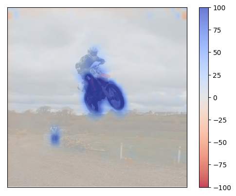
Direct comparison of explanations generated for the caption” riding a dirt bike” from different visual backbones and methods. The first two starting from the left, are generated from features extracted using DFF and activations of different visual backbones, namely a CNN (Figure 5.5.3) and ViT(Figure 5.5.3). Figure 5.5.3 uses semantic masks extracted by a segmentation model (STEGO) and 5.5.3 uses superpixel features. All the explanations have comparable compute costs, apart from Figure 5.5.3, where only features are used.
The biggest advantage of using an off-the-self segmentation model is that it supports the generation of visual explanations, independently of the visual backbone’s architecture. On the other hand, we have the downside of no longer relying on the visual backbones’ priors, embedded in the captioning model.
In Figure 2 we directly compare the visual explanations generated by all methods, DFF on CNN and ViT (Figures 5.5.3 and 5.5.3), STEGO (Figure 5.5.3), and superpixel (Figure 5.5.3). All the explanations are generated with similar compute costs, apart from STEGO which uses a smaller amount of features (). As expected, the explanations generated with STEGO’s semantic features are more fine-grained than the others, as the model is trained on the semantic segmentation task. However, they come from an external model and do not necessarily reflect the visual priors of the V&L model itself. Nevertheless, this provides a flexible solution to adapt the explanation of V&L models with visual priors to any visual backbone. Furthermore, any segmentation model can in principle be used.
Superpixel
Direct comparison of explanations generated for the caption” riding a dirt bike” from different visual backbones and methods. The first two starting from the left, are generated from features extracted using DFF and activations of different visual backbones, namely a CNN (Figure 5.5.3) and ViT(Figure 5.5.3). Figure 5.5.3 uses semantic masks extracted by a segmentation model (STEGO) and 5.5.3 uses superpixel features. All the explanations have comparable compute costs, apart from Figure 5.5.3, where only features are used.
The biggest advantage of using an off-the-self segmentation model is that it supports the generation of visual explanations, independently of the visual backbone’s architecture. On the other hand, we have the downside of no longer relying on the visual backbones’ priors, embedded in the captioning model.
In Figure 2 we directly compare the visual explanations generated by all methods, DFF on CNN and ViT (Figures 5.5.3 and 5.5.3), STEGO (Figure 5.5.3), and superpixel (Figure 5.5.3). All the explanations are generated with similar compute costs, apart from STEGO which uses a smaller amount of features (). As expected, the explanations generated with STEGO’s semantic features are more fine-grained than the others, as the model is trained on the semantic segmentation task. However, they come from an external model and do not necessarily reflect the visual priors of the V&L model itself. Nevertheless, this provides a flexible solution to adapt the explanation of V&L models with visual priors to any visual backbone. Furthermore, any segmentation model can in principle be used.
minipage0.24
6 Human Evaluation
The experiments in the previous section made direct comparisons between our method and superpixel-based explanations for V&L generative models. In this section, we report on an evaluation with human participants. Evaluating XAI techniques is a notoriously challenging task (e.g. Nauta et al., 2023; Adebayo et al., 2022). Here, we take inspiration from the work of Hoffman et al. (2018) and compare the judgments of participants on three qualities, namely detail, satisfaction and completeness of explanations generated using the two methods under consideration.
6.1 Participants
For the purposes of this study, it is important to source judgments from participants who are knowledgeable about machine learning and explainable AI. Relying on crowd-sourcing is a risky strategy, as there is no guarantee that participants will be in a position to evaluate explanations rather than, say, the quality of model outputs. We, therefore, recruited 14 researchers (9 male, 5 female; 9 aged 18-30, 4 aged 31-40, 1 aged 41-50) from our own network. All are researchers in AI-related fields and are familiar with XAI methods. Two of these are senior researchers who obtained their PhD more than 5 years ago; all the others were doctoral students at the time the experiment was run. Six participants are native speakers of English; the remainder are fluent or near-fluent speakers.

6.2 Design and materials
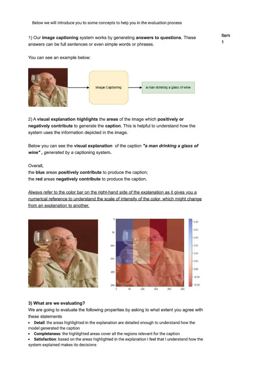
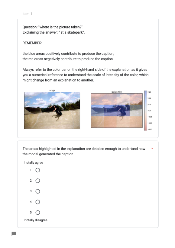
We randomly selected 40 images from the HL dataset, for which we generated the corresponding answers to questions. In order to create a more challenging scenario, we framed it into a visual question-answering task, thus for each image, we select one of the available questions and we generate the corresponding caption. Moreover, for each image-caption pair, we generated visual explanations using both DFF and superpixels features. Each participant was shown the question, the generated answer, the original image, and the visual explanation which can be either generated by DFF or by superpixel. In order to counterbalance the experimental materials, we divided images randomly into two groups, and further assigned participants randomly to two groups. We rotated items through a 2 (participant group) 2 (image group) Latin square, such that participants in any experimental group evaluated all images, but each image was always seen once and evaluated in only one condition (DFF or superpixel).333In the end, the experiment was completed by 8 participants in one group, and 6 in the other. The participants were asked to judge explanations based on their agreement to each of the following statements:
-
•
Detail: the areas highlighted in the explanation are detailed enough to understand how the model generated the caption;
-
•
Completeness: the highlighted areas cover all the regions relevant to the caption;
-
•
Satisfaction: based on the areas highlighted in the explanation I feel that I understand how the system explained makes its decisions.
Responses to each dimension were given on on a Likert scale from to , where corresponds to the total agreement and to total disagreement. The full evaluation form is reproduced in the appendix.
6.3 Results
As shown in Figure 11, DFF-based explanations (in orange) are considered on par with superpixel-based explanations (in blue) in terms of completeness, but at the same time, they are considered more detailed and more satisfactory for human judges. Thus, the score distributions for detail and satisfaction are more skewed towards lower (better) scores for the detail and satisfaction criteria. More detailed statistics are reported in Table 2.
| Type | Metric | Mean | Std | Median |
|---|---|---|---|---|
| SP | completeness | 2.48 | 1.38 | 2.0 |
| detail | 2.46 | 1.42 | 2.0 | |
| satisfaction | 2.51 | 1.51 | 2.0 | |
| DFF | completeness | 2.50 | 1.45 | 2.0 |
| detail | 2.18 | 1.41 | 2.0 | |
| satisfaction | 2.32 | 1.48 | 2.0 |
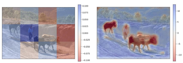
Although the superpixel and DFF differ in the judged level of detail of the explanations, they yield attributions which are similarly located in the input image. This is in part due to the fact that in both cases, we are using the same feature attribution method, namely Kernel SHAP. However, in the same cases, we observe a certain degree of divergence in the visual explanation. In Figure 12 we show an example where we generate explanations for the question “Where is the picture taken?” and the generated caption “on a dirty road”. The DFF-based explanation (on the right) broadly assigns a positive attribution to the background of the picture, depicting the road, and negative contributions to the subjects, namely the person and the animals. However, the superpixel-based explanation (on the left) assigns attributions to patches that are, at least partially, in contrast with the DFF-based explanation. This is probably due to the particular configuration of features selected by both methods, which in some instances might select insufficiently detailed regions, preventing the method from highlighting the semantically relevant areas of the image.
In order to quantify this phenomenon we manually inspected the 40 samples used in the human evaluation. We found that around of the explanations diverged to some extent between the two feature selection methods. We analyzed separately this sub-sample of divergent explanations. We find that the average scores for this subset are overall slightly worse (higher) than the full results reported in Table 2. Nevertheless, the trends observed in relation to Figure 11 for the three evaluation criteria still hold. This suggests that this phenomenon does not significantly affect the participants’ judgments, except for a slight drop in the perceived quality of the explanations. Moreover, in qualitative feedback given by participants, some declared that in some instances, their assessment was affected by the correctness of the caption, which in some cases was considered wrong or partially inaccurate. We quantified the inaccuracy of the caption by computing their lexical and semantic similarity with respect to the reference captions, using respectively, BLEU (Papineni et al., 2002) and Sentence-Bert (Reimers and Gurevych, 2019). We computed the Pearson correlation (Cohen et al., 2009) between the Likert scores and the lexical and semantic similarity previously computed. We find that the Likert scores slightly but not significantly positively correlate with both lexical and semantic similarity ( for lexical similarity and for semantic similarity)444Note that since in the Likert score, 1 is the maximum agreement and 5 the minimum, a positive correlation corresponds to a negative .. This suggests that despite the fact that participants did note the quality of the captions, this did not significantly affect their judgments of the explanations. In conclusion, we found that assessing visual explanations is a hard task even for specialists in the field. We observed a relatively low inter-annotator agreement for both groups in the Likert judgments (Krippendorff’s (Krippendorff, 2004)). However, besides possible confounding factors, like inaccuracies of the captions and divergent explanations, the DFF-based explanations are consistently perceived as higher quality explanations than superpixel-based ones.
7 Conclusions
In this work, we proposed an explainability framework to bridge the gap between multimodality and explainability in image-to-text generative tasks exploiting textual and visual semantics. Our method is developed around SHAP, as it provides a model-agnostic solution with solid theory and desirable properties. We design our approach to address certain crucial limitations of current approaches. First, SHAP-based methods are rarely employed to explain large models as they are extremely expensive to compute. Our solution is efficient and allows an accurate approximation of the Shapley values. Second, we overcome the limitations of current token-by-token explanations by proposing sentence-based explanations exploiting semantic textual variations which are also more efficient to compute. Finally, based on the rationale that a model’s generative outputs should be explained with reference to the knowledge encoded by the visual backbone, we propose an unsupervised method to extract semantically informative visual features. Using these features rather than superpixels means that we obtain explanations which are cheaper (insofar as more can be gleaned from fewer features) but also more intuitive, especially when compared to superpixel-based approaches. We show that our method can be employed with different visual-backbones architectures like CNN and Vision Transformers. In the case of visual backbones for which desirable results cannot be produced, such as FasterRCNN-based models, we propose an alternative solution based on a semantic segmentation model, to generate semantic input features. Through a human evaluation, we show that using semantic priors improves the perceived quality of the explanation, resulting in more detailed and satisfactory explanations than superpixels though matching the same level of completeness. Moreover, our framework is totally modular and it can co-exist with a wide range of possible configurations for all of its components. It allows the computation of sentence-based or token-by-token explanations. The core method, Kernel SHAP, can be replaced with another SHAP-based method, and the visual features can be extracted with one of the proposed methods or with any other method of choice.
Funding
Contribution from the ITN project NL4XAI (Natural Language for Explainable AI). This project has received funding from the European Union’s Horizon 2020 research and innovation programme under the Marie Skłodowska-Curie grant agreement No 860621. This document reflects the views of the author(s) and does not necessarily reflect the views or policy of the European Commission. The REA cannot be held responsible for any use that may be made of the information this document contains.
References
- Adebayo et al. (2022) Adebayo, J., Muelly, M., Abelson, H., and Kim, B. (2022). Post-hoc explanations may be ineffective for detecting unknown spurious correlation. In Proceedings of the 10th International Conference on Learning Representations (ICLR’22). 13
- Ahmed et al. (2021) Ahmed, U., Lin, J. C.-W., and Srivastava, G. (2021). Fuzzy explainable attention-based deep active learning on mental-health data. In 2021 IEEE International Conference on Fuzzy Systems (FUZZ-IEEE) (IEEE), 1–6
- Anderson et al. (2018) Anderson, P., He, X., Buehler, C., Teney, D., Johnson, M., Gould, S., et al. (2018). Bottom-up and top-down attention for image captioning and visual question answering. In Proceedings of the IEEE conference on computer vision and pattern recognition. 6077–6086
- Antol et al. (2015) Antol, S., Agrawal, A., Lu, J., Mitchell, M., Batra, D., Zitnick, C. L., et al. (2015). Vqa: Visual question answering. In Proceedings of the IEEE international conference on computer vision. 2425–2433
- Binder et al. (2016) Binder, A., Bach, S., Montavon, G., Müller, K.-R., and Samek, W. (2016). Layer-wise relevance propagation for deep neural network architectures. In Information science and applications (ICISA) 2016 (Springer), 913–922
- Boenninghoff et al. (2019) Boenninghoff, B., Hessler, S., Kolossa, D., and Nickel, R. M. (2019). Explainable authorship verification in social media via attention-based similarity learning. In 2019 IEEE International Conference on Big Data (Big Data) (IEEE), 36–45
- Breiman (2001) Breiman, L. (2001). Random forests. Machine learning 45, 5–32
- Cafagna et al. (2023) Cafagna, M., van Deemter, K., and Gatt, A. (2023). HL dataset: Grounding High-Level Linguistic Concepts in Vision. arXiv preprint arXiv:2302.12189
- Cao et al. (2022) Cao, M., Li, S., Li, J., Nie, L., and Zhang, M. (2022). Image-text retrieval: A survey on recent research and development. In Proceedings of the Thirty-First International Joint Conference on Artificial Intelligence, IJCAI-22, ed. L. D. Raedt (International Joint Conferences on Artificial Intelligence Organization), 5410–5417. 10.24963/ijcai.2022/759. Survey Track
- Chen et al. (2020) Chen, H., Zheng, G., and Ji, Y. (2020). Generating Hierarchical Explanations on Text Classification via Feature Interaction Detection. In Proceedings of the 58th Annual Meeting of the Association for Computational Linguistics (Online: Association for Computational Linguistics), 5578–5593. 10.18653/v1/2020.acl-main.494
- Cohen et al. (2009) Cohen, I., Huang, Y., Chen, J., Benesty, J., Benesty, J., Chen, J., et al. (2009). Pearson correlation coefficient. Noise reduction in speech processing , 1–4
- Collins et al. (2018) Collins, E., Achanta, R., and Susstrunk, S. (2018). Deep feature factorization for concept discovery. In Proceedings of the European Conference on Computer Vision (ECCV). 336–352
- Cornia et al. (2022) Cornia, M., Baraldi, L., and Cucchiara, R. (2022). Explaining transformer-based image captioning models: An empirical analysis. AI Communications 35, 111–129
- Dosovitskiy et al. (2020) Dosovitskiy, A., Beyer, L., Kolesnikov, A., Weissenborn, D., Zhai, X., Unterthiner, T., et al. (2020). An image is worth 16x16 words: Transformers for image recognition at scale. arXiv preprint arXiv:2010.11929
- Fisch et al. (2020) Fisch, A., Lee, K., Chang, M.-W., Clark, J. H., and Barzilay, R. (2020). Capwap: Captioning with a purpose. arXiv preprint arXiv:2011.04264
- Fisher et al. (2019) Fisher, A., Rudin, C., and Dominici, F. (2019). All models are wrong, but many are useful: Learning a variable’s importance by studying an entire class of prediction models simultaneously. J. Mach. Learn. Res. 20, 1–81
- Hamilton et al. (2022) Hamilton, M., Zhang, Z., Hariharan, B., Snavely, N., and Freeman, W. T. (2022). Unsupervised semantic segmentation by distilling feature correspondences. arXiv preprint arXiv:2203.08414
- Hoffman et al. (2018) Hoffman, R. R., Mueller, S. T., Klein, G., and Litman, J. (2018). Metrics for explainable ai: Challenges and prospects. arXiv preprint arXiv:1812.04608
- Hossain et al. (2019) Hossain, M. Z., Sohel, F., Shiratuddin, M. F., and Laga, H. (2019). A comprehensive survey of deep learning for image captioning. ACM Computing Surveys (CsUR) 51, 1–36
- Jeyakumar et al. (2020) Jeyakumar, J. V., Noor, J., Cheng, Y.-H., Garcia, L., and Srivastava, M. (2020). How can i explain this to you? an empirical study of deep neural network explanation methods. Advances in Neural Information Processing Systems 33, 4211–4222
- Kirillov et al. (2023) Kirillov, A., Mintun, E., Ravi, N., Mao, H., Rolland, C., Gustafson, L., et al. (2023). Segment anything. arXiv preprint arXiv:2304.02643
- Kokalj et al. (2021) Kokalj, E., Škrlj, B., Lavrač, N., Pollak, S., and Robnik-Šikonja, M. (2021). Bert meets shapley: Extending shap explanations to transformer-based classifiers. In Proceedings of the EACL Hackashop on News Media Content Analysis and Automated Report Generation. 16–21
- Krippendorff (2004) Krippendorff, K. (2004). Reliability in content analysis: Some common misconceptions and recommendations. Human communication research 30, 411–433
- Lei et al. (2018) Lei, J., G’Sell, M., Rinaldo, A., Tibshirani, R. J., and Wasserman, L. (2018). Distribution-free predictive inference for regression. Journal of the American Statistical Association 113, 1094–1111
- Li et al. (2022a) Li, J., Li, D., Xiong, C., and Hoi, S. (2022a). Blip: Bootstrapping language-image pre-training for unified vision-language understanding and generation. In International Conference on Machine Learning (PMLR), 12888–12900
- Li et al. (2021) Li, L., Wang, B., Verma, M., Nakashima, Y., Kawasaki, R., and Nagahara, H. (2021). Scouter: Slot attention-based classifier for explainable image recognition. In Proceedings of the IEEE/CVF International Conference on Computer Vision. 1046–1055
- Li et al. (2022b) Li, Y., Li, C., Li, X., Wang, K., Rahaman, M. M., Sun, C., et al. (2022b). A comprehensive review of markov random field and conditional random field approaches in pathology image analysis. Archives of Computational Methods in Engineering 29, 609–639
- Lin et al. (2014) Lin, T.-Y., Maire, M., Belongie, S., Hays, J., Perona, P., Ramanan, D., et al. (2014). Microsoft coco: Common objects in context. In Computer Vision–ECCV 2014: 13th European Conference, Zurich, Switzerland, September 6-12, 2014, Proceedings, Part V 13 (Springer), 740–755
- Loyola-Gonzalez (2019) Loyola-Gonzalez, O. (2019). Black-box vs. white-box: Understanding their advantages and weaknesses from a practical point of view. IEEE access 7, 154096–154113
- Lundberg and Lee (2017) Lundberg, S. M. and Lee, S.-I. (2017). A unified approach to interpreting model predictions. Advances in neural information processing systems 30
- Mokady et al. (2021) Mokady, R., Hertz, A., and Bermano, A. H. (2021). Clipcap: Clip prefix for image captioning. arXiv preprint arXiv:2111.09734
- Molnar (2020) Molnar, C. (2020). Interpretable machine learning (Lulu. com)
- Mosca et al. (2022a) Mosca, E., Szigeti, F., Tragianni, S., Gallagher, D., and Groh, G. (2022a). Shap-based explanation methods: A review for nlp interpretability. In Proceedings of the 29th International Conference on Computational Linguistics. 4593–4603
- Mosca et al. (2022b) Mosca, E., Szigeti, F., Tragianni, S., Gallagher, D., and Groh, G. (2022b). SHAP-based explanation methods: A review for NLP interpretability. In Proceedings of the 29th International Conference on Computational Linguistics (Gyeongju, Republic of Korea: International Committee on Computational Linguistics), 4593–4603
- Nauta et al. (2023) Nauta, M., Trienes, J., Pathak, S., Nguyen, E., Peters, M., Schmitt, Y., et al. (2023). From Anecdotal Evidence to Quantitative Evaluation Methods: A Systematic Review on Evaluating Explainable AI. ACM Computing Surveys 10.1145/3583558
- Papineni et al. (2002) Papineni, K., Roukos, S., Ward, T., and Zhu, W.-J. (2002). Bleu: a method for automatic evaluation of machine translation. In Proceedings of the 40th annual meeting of the Association for Computational Linguistics. 311–318
- Parcalabescu et al. (2022) Parcalabescu, L., Cafagna, M., Muradjan, L., Frank, A., Calixto, I., and Gatt, A. (2022). VALSE: A task-independent benchmark for vision and language models centered on linguistic phenomena. In Proceedings of the 60th Annual Meeting of the Association for Computational Linguistics (Volume 1: Long Papers) (Dublin, Ireland: Association for Computational Linguistics), 8253–8280. 10.18653/v1/2022.acl-long.567
- Parcalabescu and Frank (2022) Parcalabescu, L. and Frank, A. (2022). Mm-shap: A performance-agnostic metric for measuring multimodal contributions in vision and language models & tasks. arXiv preprint arXiv:2212.08158
- Park et al. (2020) Park, J. S., Bhagavatula, C., Mottaghi, R., Farhadi, A., and Choi, Y. (2020). Visualcomet: Reasoning about the dynamic context of a still image. In Computer Vision–ECCV 2020: 16th European Conference, Glasgow, UK, August 23–28, 2020, Proceedings, Part V 16 (Springer), 508–524
- Petsiuk et al. (2018) Petsiuk, V., Das, A., and Saenko, K. (2018). Rise: Randomized input sampling for explanation of black-box models. arXiv preprint arXiv:1806.07421
- Radford et al. (2021) Radford, A., Kim, J. W., Hallacy, C., Ramesh, A., Goh, G., Agarwal, S., et al. (2021). Learning transferable visual models from natural language supervision. In International conference on machine learning (PMLR), 8748–8763
- Reimers and Gurevych (2019) Reimers, N. and Gurevych, I. (2019). Sentence-bert: Sentence embeddings using siamese bert-networks. arXiv preprint arXiv:1908.10084
- Ren et al. (2015) Ren, S., He, K., Girshick, R., and Sun, J. (2015). Faster r-cnn: Towards real-time object detection with region proposal networks. Advances in neural information processing systems 28
- Ribeiro et al. (2016) Ribeiro, M. T., Singh, S., and Guestrin, C. (2016). Model-agnostic interpretability of machine learning. arXiv preprint arXiv:1606.05386
- Selvaraju et al. (2017) Selvaraju, R. R., Cogswell, M., Das, A., Vedantam, R., Parikh, D., and Batra, D. (2017). Grad-cam: Visual explanations from deep networks via gradient-based localization. In Proceedings of the IEEE international conference on computer vision. 618–626
- Shapley et al. (1953) Shapley, L. S. et al. (1953). A value for n-person games
- Sharma et al. (2020) Sharma, H., Agrahari, M., Singh, S. K., Firoj, M., and Mishra, R. K. (2020). Image captioning: a comprehensive survey. In 2020 International Conference on Power Electronics & IoT Applications in Renewable Energy and its Control (PARC) (IEEE), 325–328
- Shrikumar et al. (2017) Shrikumar, A., Greenside, P., and Kundaje, A. (2017). Learning important features through propagating activation differences. In International conference on machine learning (PMLR), 3145–3153
- Shrikumar et al. (2016) Shrikumar, A., Greenside, P., Shcherbina, A., and Kundaje, A. (2016). Not just a black box: Learning important features through propagating activation differences. arXiv preprint arXiv:1605.01713
- Simonyan et al. (2013) Simonyan, K., Vedaldi, A., and Zisserman, A. (2013). Deep inside convolutional networks: Visualising image classification models and saliency maps. arXiv preprint arXiv:1312.6034
- Springenberg et al. (2014) Springenberg, J. T., Dosovitskiy, A., Brox, T., and Riedmiller, M. (2014). Striving for simplicity: The all convolutional net. arXiv preprint arXiv:1412.6806
- Srivastava et al. (2021) Srivastava, Y., Murali, V., Dubey, S. R., and Mukherjee, S. (2021). Visual question answering using deep learning: A survey and performance analysis. In Computer Vision and Image Processing: 5th International Conference, CVIP 2020, Prayagraj, India, December 4-6, 2020, Revised Selected Papers, Part II 5 (Springer), 75–86
- Sundararajan et al. (2017) Sundararajan, M., Taly, A., and Yan, Q. (2017). Axiomatic attribution for deep networks. In International conference on machine learning (PMLR), 3319–3328
- Tan and Bansal (2019) Tan, H. and Bansal, M. (2019). Lxmert: Learning cross-modality encoder representations from transformers. arXiv preprint arXiv:1908.07490
- Teneggi et al. (2022) Teneggi, J., Luster, A., and Sulam, J. (2022). Fast Hierarchical Games for Image Explanations. IEEE Transactions on Pattern Analysis and Machine Intelligence , 1–1110.1109/TPAMI.2022.3189849. ArXiv:2104.06164 [cs]
- Thrush et al. (2022) Thrush, T., Jiang, R., Bartolo, M., Singh, A., Williams, A., Kiela, D., et al. (2022). Winoground: Probing vision and language models for visio-linguistic compositionality. In Proceedings of the IEEE/CVF Conference on Computer Vision and Pattern Recognition. 5238–5248
- Wang et al. (2022) Wang, P., Yang, A., Men, R., Lin, J., Bai, S., Li, Z., et al. (2022). Unifying architectures, tasks, and modalities through a simple sequence-to-sequence learning framework. arXiv preprint arXiv:2202.03052
- Webber et al. (2010) Webber, W., Moffat, A., and Zobel, J. (2010). A similarity measure for indefinite rankings. ACM Transactions on Information Systems (TOIS) 28, 1–38
- Yu et al. (2016) Yu, L., Poirson, P., Yang, S., Berg, A. C., and Berg, T. L. (2016). Modeling context in referring expressions. In Computer Vision–ECCV 2016: 14th European Conference, Amsterdam, The Netherlands, October 11-14, 2016, Proceedings, Part II 14 (Springer), 69–85
- Zeiler and Fergus (2014) Zeiler, M. D. and Fergus, R. (2014). Visualizing and understanding convolutional networks. In Computer Vision–ECCV 2014: 13th European Conference, Zurich, Switzerland, September 6-12, 2014, Proceedings, Part I 13 (Springer), 818–833
- Zellers et al. (2019) Zellers, R., Bisk, Y., Farhadi, A., and Choi, Y. (2019). From recognition to cognition: Visual commonsense reasoning. In Proceedings of the IEEE/CVF conference on computer vision and pattern recognition. 6720–6731
- Zhang et al. (2019a) Zhang, C., Gao, F., Jia, B., Zhu, Y., and Zhu, S.-C. (2019a). Raven: A dataset for relational and analogical visual reasoning. In Proceedings of the IEEE/CVF conference on computer vision and pattern recognition. 5317–5327
- Zhang et al. (2021) Zhang, P., Li, X., Hu, X., Yang, J., Zhang, L., Wang, L., et al. (2021). Vinvl: Revisiting visual representations in vision-language models. In Proceedings of the IEEE/CVF Conference on Computer Vision and Pattern Recognition. 5579–5588
- Zhang et al. (2019b) Zhang, Y., Niebles, J. C., and Soto, A. (2019b). Interpretable visual question answering by visual grounding from attention supervision mining. In 2019 ieee winter conference on applications of computer vision (wacv) (IEEE), 349–357
- Zheng et al. (2022) Zheng, J., Qin, Z., Wang, S., and Li, D. (2022). Attention-based explainable friend link prediction with heterogeneous context information. Information Sciences 597, 211–229
- Zhu et al. (2016) Zhu, Y., Groth, O., Bernstein, M., and Fei-Fei, L. (2016). Visual7w: Grounded question answering in images. In Proceedings of the IEEE conference on computer vision and pattern recognition. 4995–5004
8 Supplementary Tables and Figures
