The Exponential Capacity of Dense Associative Memories

Carlo Lucibello carlo.lucibello@unibocconi.it    Marc Mézard marc.mezard@unibocconi.it Department of Computing Sciences, Bocconi University, Milano, Italy
Bocconi Institute for Data Science and Analytics (BIDSA), Milano, Italy
Abstract

Recent generalizations of the Hopfield model of associative memories are able to store a number P𝑃P of random patterns that grows exponentially with the number N𝑁N of neurons, P=exp(αN)𝑃𝛼𝑁P=\exp(\alpha N). Besides the huge storage capacity, another interesting feature of these networks is their connection to the attention mechanism which is part of the Transformer architectures widely applied in deep learning. In this work, we study a generic family of pattern ensembles using a statistical mechanics analysis which gives exact asymptotic thresholds for the retrieval of a typical pattern, α1subscript𝛼1\alpha_{1}, and lower bounds for the maximum of the load α𝛼\alpha for which all patterns can be retrieved, αcsubscript𝛼𝑐\alpha_{c}, as well as sizes of attraction basins. We discuss in detail the cases of Gaussian and spherical patterns, and show that they display rich and qualitatively different phase diagrams.

I Introduction

About forty years ago, John Hopfield introduced a simple model of memory [1] based on N𝑁N spins interacting by pairs like in a spin glass, but with specifically tailored interactions so that the ground states of the spin-glass are strongly correlated with a set of patterns that one wants to memorize. This allows building an associative memory that retrieves the full information from some partial information. Using statistical physics methods, it was then shown that this model can store up to αcNsubscript𝛼𝑐𝑁\alpha_{c}N independent random patterns in the large N𝑁N limit, with αc0.14similar-to-or-equalssubscript𝛼𝑐0.14\alpha_{c}\simeq 0.14 if one uses the simple Hebb rule for defining the interactions [2, 3]. Going beyond pairwise interactions, i.e. introducing p𝑝p-spin interactions, yields a big increase in the memory capacity which becomes of order Np1superscript𝑁𝑝1N^{p-1} [4, 5, 6]. Pushing this strategy further, a family of models with exponential interaction terms leading to exponential capacity has been recently introduced and analyzed in Refs. [7, 8]. While [7] discusses networks with Ising variables, Ref. [8] considers continuous variables and links the dynamics of the system with the attention mechanism one finds in the transformer models [9] now ubiquitous in natural language processing and other domains in machine learning. We refer to all these generalization as Dense Associative Memories (DAMs). Here we perform a statistical mechanics analysis of the DAM with continuous variables introduced in [8]. We expect that a similar approach can be used in the case [7] of discrete variables and other DAMs. Defining P=eαN𝑃superscript𝑒𝛼𝑁P=e^{\alpha N} as the number of patterns, we want to compute the critical value αcsubscript𝛼𝑐\alpha_{c} such that, for α<αc𝛼subscript𝛼𝑐\alpha<\alpha_{c} retrieval is possible with high probability in the large N𝑁N limit. Notice that the precise definition of αcsubscript𝛼𝑐\alpha_{c} in presence of an exponentially large number of patterns requires some care, and indeed we will find distinct thresholds depending on whether we request to store all patterns, or we request that a randomly chosen pattern can be retrieved with probability one.

Following [8], we consider a set of P=eαN𝑃superscript𝑒𝛼𝑁P=e^{\alpha N} patterns {𝝃μ}μ=1Psuperscriptsubscriptsuperscript𝝃𝜇𝜇1𝑃\{\operatorname{\bm{\xi}}^{\mu}\}_{\mu=1}^{P}, 𝝃μNsuperscript𝝃𝜇superscript𝑁\operatorname{\bm{\xi}}^{\mu}\in\mathbb{R}^{N}, independently and identically distributed according to some distribution 𝒫(𝝃)𝒫𝝃\mathcal{P}(\operatorname{\bm{\xi}}), normalized such that 𝔼𝝃2=N𝔼superscriptdelimited-∥∥𝝃2𝑁\mathbb{E}\lVert\operatorname{\bm{\xi}}\rVert^{2}=N. These patterns should be memorized by a network of N𝑁N neurons, with activities encoded in a N𝑁N-dimensional vector 𝐱𝐱\operatorname{\mathbf{x}}. Starting from an initial condition 𝐱0Nsubscript𝐱0superscript𝑁\operatorname{\mathbf{x}}_{0}\in\mathbb{R}^{N}, the recall of a memorized pattern is based on a gradient descent of the energy function

E(𝐱)𝐸𝐱\displaystyle E(\operatorname{\mathbf{x}}) =1λlogμ=1Peλ𝐱𝝃μ+12𝐱2,\displaystyle=-\frac{1}{\lambda}\log\sum_{\mu=1}^{P}e^{\lambda\operatorname{\mathbf{x}}\cdot\operatorname{\bm{\xi}}^{\mu}}+\frac{1}{2}\lVert\operatorname{\mathbf{x}}\lVert^{2}, (1)

Notice that with respect to Ref. [8] we exchanged the roles of 𝐱𝐱\operatorname{\mathbf{x}} and 𝝃𝝃\operatorname{\bm{\xi}} in order to conform to statistical physics’ standard notation. The gradient descent with learning rate one gives:

𝐱t+1=subscript𝐱𝑡1absent\displaystyle\operatorname{\mathbf{x}}_{t+1}= μatμ𝝃μ,atμ=eλ𝐱t𝝃μνeλ𝐱t𝝃ν.subscript𝜇superscriptsubscript𝑎𝑡𝜇superscript𝝃𝜇superscriptsubscript𝑎𝑡𝜇superscript𝑒𝜆subscript𝐱𝑡superscript𝝃𝜇subscript𝜈superscript𝑒𝜆subscript𝐱𝑡superscript𝝃𝜈\displaystyle\sum_{\mu}a_{t}^{\mu}\,\operatorname{\bm{\xi}}^{\mu}\;,\qquad a_{t}^{\mu}=\frac{e^{\lambda\operatorname{\mathbf{x}}_{t}\cdot\operatorname{\bm{\xi}}^{\mu}}}{\sum_{\nu}e^{\lambda\operatorname{\mathbf{x}}_{t}\cdot\operatorname{\bm{\xi}}^{\nu}}}\;. (2)

Interestingly, this update rule is well known in deep learning [10, 9]. It corresponds to a cross-attention mechanism with a single query 𝐱=𝐪𝐱𝐪\operatorname{\mathbf{x}}=\mathbf{q} and identical key and value matrices: K=V=[𝝃1,,𝝃P]𝐾𝑉superscript𝝃1superscript𝝃𝑃K=V=[\operatorname{\bm{\xi}}^{1},...,\operatorname{\bm{\xi}}^{P}]. The update rule can be compactly written as 𝐱t+1=VSoftmax(𝐱tTK)subscript𝐱𝑡1𝑉Softmaxsuperscriptsubscript𝐱𝑡𝑇𝐾\operatorname{\mathbf{x}}_{t+1}=V\operatorname{Softmax}(\operatorname{\mathbf{x}}_{t}^{T}K). The coefficients atμsuperscriptsubscript𝑎𝑡𝜇a_{t}^{\mu} are called attention scores.

A pattern 𝝃μsuperscript𝝃𝜇\operatorname{\bm{\xi}}^{\mu} will be said to be retrieved if, starting from an initial configuration 𝐱0subscript𝐱0\operatorname{\mathbf{x}}_{0} close enough to the pattern, the gradient iterations converge close to the pattern: limt1N𝐱t𝝃μ2<ϵsubscript𝑡1𝑁superscriptdelimited-∥∥subscript𝐱𝑡superscript𝝃𝜇2italic-ϵ\lim_{t\to\infty}\frac{1}{N}\lVert\operatorname{\mathbf{x}}_{t}-\operatorname{\bm{\xi}}^{\mu}\rVert^{2}<\epsilon for some constant ϵ>0italic-ϵ0\epsilon>0 that we assume to be vanishing in the limit of large N𝑁N. In the standard Hopfield model with P=O(N)𝑃𝑂𝑁P=O(N) patterns, the retrieved configuration always contains a small fraction of errors compared to the original pattern, and one has to impose P=O(N/log(N))𝑃𝑂𝑁𝑁P=O(N/\log(N)) for perfect retrieval [11]. For our DAM, we discuss (asymptotic) perfect retrieval.

At fixed interaction strength λ𝜆\lambda, we define the single pattern retrieval threshold α1(λ)subscript𝛼1𝜆\alpha_{1}(\lambda) as the largest value of α𝛼\alpha for which the probability of retrieving a randomly chosen pattern goes to one in the large N𝑁N limit. This is a sharp phase transition: as we shall see, for α>α1(λ)𝛼subscript𝛼1𝜆\alpha>\alpha_{1}(\lambda) this probability goes to zero. The other problem we consider is the full retrieval problem, that is determining the maximum number of patterns that are jointly stored. We define the capacity threshold αc(λ)subscript𝛼𝑐𝜆\alpha_{c}(\lambda) as the largest α𝛼\alpha such that all P=eαN𝑃superscript𝑒𝛼𝑁P=e^{\alpha N} patterns are retrieved. Clearly we have αc(λ)α1(λ)subscript𝛼𝑐𝜆subscript𝛼1𝜆\alpha_{c}(\lambda)\leq\alpha_{1}(\lambda).

In this paper, we derive exact and simple expressions for α1(λ)subscript𝛼1𝜆\alpha_{1}(\lambda), provide bounds on αc(λ)subscript𝛼𝑐𝜆\alpha_{c}(\lambda), and study the size of attraction basins, i.e. the maximal distance between 𝐱0subscript𝐱0\operatorname{\mathbf{x}}_{0} and the pattern such that retrieval is possible. We shall first explain the general formalism and then apply it to various distributions of patterns.

II Retrieval of a typical pattern

We study the capacity in the thermodynamic limit N𝑁N\to\infty. Let us choose one of the patterns independently from the sample realization, say 𝝃1superscript𝝃1\bm{\xi}^{1}, and explore the energy landscape E(𝐱)𝐸𝐱E(\operatorname{\mathbf{x}}) in its neighborhood, when the overlap 𝐱𝝃1𝐱superscript𝝃1\operatorname{\mathbf{x}}\cdot\operatorname{\bm{\xi}}^{1}, as well as the square norm 𝐱2superscriptnorm𝐱2\|\operatorname{\mathbf{x}}\|^{2} are of O(N)𝑂𝑁O(N). The overlaps of 𝐱𝐱\operatorname{\mathbf{x}} with each of the eαN1superscript𝑒𝛼𝑁1e^{\alpha N}-1 other patterns are typically of order N𝑁\sqrt{N}; however, as their number is exponentially large, some of these overlaps will also be of order N𝑁N. It is convenient to rewrite the energy as:

E(𝐱)=1λlog(eλ𝐱𝝃1+eλNΦ(𝐱))+12𝐱2,E(\operatorname{\mathbf{x}})=-\frac{1}{\lambda}\log\left(e^{\lambda\operatorname{\mathbf{x}}\cdot\operatorname{\bm{\xi}}^{1}}+e^{\lambda N\Phi(\mathbf{x})}\right)+\frac{1}{2}\lVert\operatorname{\mathbf{x}}\lVert^{2}, (3)

where

Φ(𝐱)=1λNlog(μ=2Peλ𝐱𝝃μ).Φ𝐱1𝜆𝑁superscriptsubscript𝜇2𝑃superscript𝑒𝜆𝐱superscript𝝃𝜇\Phi(\operatorname{\mathbf{x}})=\frac{1}{\lambda N}\log\left(\sum_{\mu=2}^{P}e^{\lambda\operatorname{\mathbf{x}}\cdot\operatorname{\bm{\xi}}^{\mu}}\right)\ . (4)

The log\log term in the energy is the sum of two terms which are both exponential in N𝑁N. We identify the first term eλ𝐱𝝃1superscript𝑒𝜆𝐱superscript𝝃1e^{\lambda\operatorname{\mathbf{x}}\cdot\operatorname{\bm{\xi}}^{1}} as signal and eNΦ(𝐱)superscript𝑒𝑁Φ𝐱e^{N\Phi(\operatorname{\mathbf{x}})} as noise. In fact, if ΦΦ\Phi can be neglected, the energy becomes a quadratic function with minimum in 𝝃1superscript𝝃1\operatorname{\bm{\xi}}^{1}.

We now study the noise term. For given 𝝃1superscript𝝃1\operatorname{\bm{\xi}}^{1} and 𝐱𝐱\operatorname{\mathbf{x}} independent from the other patterns, ΦΦ\Phi is a random variable whose distribution is induced by the random patterns 𝝃μsuperscript𝝃𝜇\operatorname{\bm{\xi}}^{\mu} with μ=2,,P𝜇2𝑃\mu=2,...,P. Notice that ΦΦ\Phi is minus the free energy density of a Random Energy Model (REM) [12] with P1𝑃1P-1 “energies” εμ=𝐱𝝃μ/Nsuperscript𝜀𝜇𝐱superscript𝝃𝜇𝑁{\varepsilon}^{\mu}=\operatorname{\mathbf{x}}\cdot\operatorname{\bm{\xi}}^{\mu}/N and “inverse temperature” λ𝜆\lambda. Let us stress that these energies and temperature are auxiliary quantities defined within the REM, they have nothing to do with the energy function or temperature of the associative memory under study.

As recalled in Appendix A, the REM can be solved both with direct probabilistic methods and with the replica method. For the sake of the analysis, we shall focus hereafter on settings where the distribution of εμsuperscript𝜀𝜇{\varepsilon}^{\mu} depends on 𝐱𝐱\operatorname{\mathbf{x}} only through its rescaled norm ρ=𝐱/N𝜌delimited-∥∥𝐱𝑁\rho=\lVert\operatorname{\mathbf{x}}\rVert/\sqrt{N}. This is the case for pattern distributions that are rotationally invariant. In the thermodynamic limit where N,P𝑁𝑃N,P\to\infty with fixed exponential rate α𝛼\alpha and considering a sequence of 𝐱𝐱\operatorname{\mathbf{x}} chosen independently from {𝝃μ}μ=2Psuperscriptsubscriptsuperscript𝝃𝜇𝜇2𝑃\{\operatorname{\bm{\xi}}^{\mu}\}_{\mu=2}^{P} and at fixed ρ=𝐱/N𝜌norm𝐱𝑁\rho=\|\operatorname{\mathbf{x}}\|/\sqrt{N}, the quantity Φ(𝐱)Φ𝐱\Phi(\operatorname{\mathbf{x}}) converges almost surely to a value ϕα,ρ(λ)subscriptitalic-ϕ𝛼𝜌𝜆\phi_{\alpha,\rho}(\lambda). This asymptotic free energy can be expressed in terms of the cumulant generating function of the εμsuperscript𝜀𝜇{\varepsilon}^{\mu}. In the case of Gaussian patterns, it reads:

ϕα,ρ(λ)={αλ+12λρ2λ<λ(α,ρ)ρ2αλλ(α,ρ),subscriptitalic-ϕ𝛼𝜌𝜆cases𝛼𝜆12𝜆superscript𝜌2𝜆subscript𝜆𝛼𝜌𝜌2𝛼𝜆subscript𝜆𝛼𝜌\displaystyle\phi_{\alpha,\rho}(\lambda)=\begin{cases}\frac{\alpha}{\lambda}+\frac{1}{2}\lambda\rho^{2}&\lambda<\lambda_{*}(\alpha,\rho)\\ \rho\sqrt{2\alpha}&\lambda\geq\lambda_{*}(\alpha,\rho),\end{cases} (5)

where λ(α,ρ)=2α/ρsubscript𝜆𝛼𝜌2𝛼𝜌\lambda_{*}(\alpha,\rho)=\sqrt{2\alpha}/\rho. The generic expression is given in (28). In general, ϕα,ρ(λ)subscriptitalic-ϕ𝛼𝜌𝜆\phi_{\alpha,\rho}(\lambda) is a decreasing function of λ𝜆\lambda and an increasing function of α𝛼\alpha. As exemplified in the Gaussian case (5), it takes two different forms separated by a glass phase transition line in the plane (α,λ)𝛼𝜆(\alpha,\lambda). For λ<λ(α,ρ)𝜆subscript𝜆𝛼𝜌\lambda<\lambda_{*}(\alpha,\rho), exponentially many energies εμsuperscript𝜀𝜇{\varepsilon}^{\mu} contribute to Φ(x)Φ𝑥\Phi(x); on the other hand, for λλ(α,ρ)𝜆subscript𝜆𝛼𝜌\lambda\geq\lambda_{*}(\alpha,\rho), the REM is dominated by the largest εμsuperscript𝜀𝜇{\varepsilon}^{\mu}: this is called condensation.

We now use this REM analysis in order to study the energy landscape of (3). For large N𝑁N we have:

E(𝐱)max(𝐱𝝃1,Nϕα,ρ(λ))+12𝐱2.E(\operatorname{\mathbf{x}})\approx-\max(\operatorname{\mathbf{x}}\cdot\operatorname{\bm{\xi}}^{1},\,N\phi_{\alpha,\rho}(\lambda))+\frac{1}{2}\lVert\operatorname{\mathbf{x}}\lVert^{2}. (6)

Whenever 𝐱𝝃1𝐱superscript𝝃1\operatorname{\mathbf{x}}\cdot\operatorname{\bm{\xi}}^{1} dominates the max\max, the energy E(𝐱)𝐸𝐱E(\operatorname{\mathbf{x}}) is a quadratic well with a minimum in 𝐱=𝝃1𝐱superscript𝝃1\operatorname{\mathbf{x}}=\operatorname{\bm{\xi}}^{1}, and the pattern 𝝃1superscript𝝃1\operatorname{\bm{\xi}}^{1} is retrieved in one step of gradient descent. This occurs at small α𝛼\alpha. When the storage α𝛼\alpha increases, ϕα,ρ(λ))\phi_{\alpha,\rho}(\lambda)) increases and the basin of attraction of 𝝃1superscript𝝃1\operatorname{\bm{\xi}}^{1} shrinks. Above a critical value of α𝛼\alpha, the quadratic well disappears, because E(𝐱=𝝃1)𝐸𝐱superscript𝝃1E(\operatorname{\mathbf{x}}=\operatorname{\bm{\xi}}^{1}) is dominated by the noise term. We thus have a simple criterion to identify the critical value α1subscript𝛼1\alpha_{1} such that for α<α1𝛼subscript𝛼1\alpha<\alpha_{1} retrieval of 𝝃1superscript𝝃1\operatorname{\bm{\xi}}^{1} is possible:

α1(λ)=sup{α:ϕα,1(λ)<1}.subscript𝛼1𝜆supremumconditional-set𝛼subscriptitalic-ϕ𝛼1𝜆1\alpha_{1}(\lambda)=\sup\left\{\,\alpha\,:\,\phi_{\alpha,1}(\lambda)<1\,\right\}. (7)

Notice that we set ρ=1𝜌1\rho=1 since 𝔼𝝃12=N𝔼superscriptdelimited-∥∥superscript𝝃12𝑁\mathbb{E}\lVert\operatorname{\bm{\xi}}^{1}\rVert^{2}=N. What happens at α>α1𝛼subscript𝛼1\alpha>\alpha_{1} when the pattern is not retrieved? Ramsauer et al. [8] show that in this case the attention scores become approximately flat and the dynamics converges to the barycenter of the patterns. In fact, it can be shown that in our high-dimensional regime E(𝐱)𝐸𝐱\nabla E(\operatorname{\mathbf{x}}) develops an extensive radial component leading the dynamics towards the origin.

Remarkably, we could derive the exact threshold α1subscript𝛼1\alpha_{1} thanks to a simple inspection of the energy function, bypassing calculations involving the dynamical rule or even quenched free energy computations à la Ref. [13]. This is a consequence of the exponentially many terms appearing in the expression of the energy, thanks to which the signal-vs-noise balance becomes an all-or-nothing one. On the other hand, let us mention a subtlety of the derivation: in the REM analysis of Φ(𝐱)Φ𝐱\Phi(\operatorname{\mathbf{x}}), we assumed the choice of 𝐱𝐱\operatorname{\mathbf{x}} to be independent from {𝝃μ}μ=2Psuperscriptsubscriptsuperscript𝝃𝜇𝜇2𝑃\{\operatorname{\bm{\xi}}^{\mu}\}_{\mu=2}^{P}. Therefore this analysis does not prove that Eq. (6) holds for all 𝐱𝐱\operatorname{\mathbf{x}} in a neighborhood of 𝝃1superscript𝝃1\operatorname{\bm{\xi}}^{1}. However, it does hold for 𝐱=𝝃1𝐱superscript𝝃1\operatorname{\mathbf{x}}=\operatorname{\bm{\xi}}^{1}, and by continuity we can deduce that, for α<α1(λ)𝛼subscript𝛼1𝜆\alpha<\alpha_{1}(\lambda), there exists a ball centered at 𝝃1superscript𝝃1\operatorname{\bm{\xi}}^{1} with a non-vanishing (and extensive) radius, such that the dynamics converges to the pattern for all 𝐱𝐱\operatorname{\mathbf{x}} inside this ball.

III Retrieval of all patterns
Refer to caption
Refer to caption
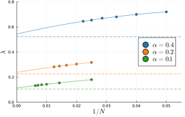
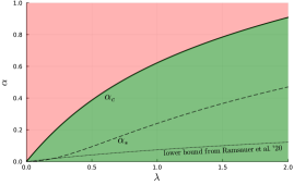
Figure 1: Top: Phase diagram for patterns uniformly distributed on the hypersphere. All the patterns are retrieved in the green region α<αc=αclb=α1𝛼subscript𝛼𝑐superscriptsubscript𝛼clbsubscript𝛼1\alpha<\alpha_{c}=\operatorname{\alpha_{c}^{lb}}=\alpha_{1} (the two thresholds coincide in the spherical setting). The dashed line α(λ)subscript𝛼𝜆\alpha_{*}(\lambda) is where the REM condensation occurs, and the dotted one is the lower bound for the capacity derived in Ref. [8]. Bottom: Gradient descent simulations starting from initial condition 𝝃1superscript𝝃1\operatorname{\bm{\xi}}^{1}. Points give values of λ𝜆\lambda where we observe a crossover between retrieval (higher λ𝜆\lambda) and non-retrieval (lower λ𝜆\lambda). Solid lines are empirical quadratic fits in 1/N1𝑁1/N. Horizontal lines are the predictions from our N=+𝑁N=+\infty theory.

We now consider the stronger requirement that all patterns can be successfully retrieved. While in the standard Hopfield model and its polynomial generalizations, single and all-patterns retrieval thresholds coincide, in presence of an exponential number of patterns one needs to control exponentially rare events.

In order to derive a lower bound, αclbαcsuperscriptsubscript𝛼clbsubscript𝛼𝑐\operatorname{\alpha_{c}^{lb}}\leq\alpha_{c}, for the critical value of α𝛼\alpha such that all patterns are retrieved, we use a union bound: if p1subscript𝑝1p_{1} is the probability of retrieving a typical pattern, the probability pcsubscript𝑝𝑐p_{c} that all patterns are retrieved verifies 1pceαN(1p1)1subscript𝑝𝑐superscript𝑒𝛼𝑁1subscript𝑝11-p_{c}\leq e^{\alpha N}(1-p_{1}). As we have seen, 1p11subscript𝑝11-p_{1} is the probability that the free-energy of the REM with P1𝑃1P-1 energy levels εμ=𝝃1𝝃μ/Nsuperscript𝜀𝜇superscript𝝃1superscript𝝃𝜇𝑁{\varepsilon}^{\mu}=\operatorname{\bm{\xi}}^{1}\cdot\operatorname{\bm{\xi}}^{\mu}/N (with μ1𝜇1\mu\neq 1) is larger than 𝝃12/Nsuperscriptdelimited-∥∥superscript𝝃12𝑁\lVert\operatorname{\bm{\xi}}^{1}\rVert^{2}/N. In order to control pcsubscript𝑝𝑐p_{c}, we thus need to compose the large deviations of the norm of the reference pattern with those of the REM free-energy.

As proven in Ref. [14] (see also [15]), if 𝝃1=rNdelimited-∥∥superscript𝝃1𝑟𝑁\lVert\operatorname{\bm{\xi}}^{1}\rVert=r\sqrt{N} and the cumulant generating function is defined for all λ𝜆\lambda\in\operatorname{\mathbb{R}}, differentiable, and strictly convex, then the distribution of the REM free-energy density ϕitalic-ϕ\phi satisfies a large deviation principle given by P(ϕ)=eNIα,r,λ(ϕ)𝑃italic-ϕsuperscript𝑒𝑁subscript𝐼𝛼𝑟𝜆italic-ϕP(\phi)=e^{-NI_{\alpha,r,\lambda}(\phi)} with

Iα,r,λ(ϕ)={+ϕ<ϕα,r(λ)0ϕ=ϕα,r(λ)sr(ϕ)αϕ>ϕα,r(λ).subscript𝐼𝛼𝑟𝜆italic-ϕcasesitalic-ϕsubscriptitalic-ϕ𝛼𝑟𝜆0italic-ϕsubscriptitalic-ϕ𝛼𝑟𝜆subscript𝑠𝑟italic-ϕ𝛼italic-ϕsubscriptitalic-ϕ𝛼𝑟𝜆I_{\alpha,r,\lambda}(\phi)=\begin{cases}+\infty&\phi<\phi_{\alpha,r}(\lambda)\\ 0&\phi=\phi_{\alpha,r}(\lambda)\\ s_{r}(\phi)-\alpha&\phi>\phi_{\alpha,r}(\lambda).\end{cases} (8)

where srsubscript𝑠𝑟s_{r} is defined in Eq. (25). Let us call I~(r)~𝐼𝑟\tilde{I}(r) instead the rate function for large deviations of 𝝃1/Ndelimited-∥∥superscript𝝃1𝑁\lVert\operatorname{\bm{\xi}}^{1}\rVert/\sqrt{N}. Accounting for the fluctuations of r𝑟r and of the REM free energy conditioned on the value of r𝑟r, it is easy to show that 1p1=eNA(α,λ)1subscript𝑝1superscript𝑒𝑁𝐴𝛼𝜆1-p_{1}=e^{-NA(\alpha,\lambda)} for large N𝑁N, where

A(α,λ)=infr[0,)[I~(r)+infϕ:ϕ>r2Iα,r,λ(ϕ)].𝐴𝛼𝜆subscriptinfimum𝑟0delimited-[]~𝐼𝑟subscriptinfimum:italic-ϕitalic-ϕsuperscript𝑟2subscript𝐼𝛼𝑟𝜆italic-ϕ\displaystyle A(\alpha,\lambda)=\inf_{r\in[0,\infty)}\left[\,\tilde{I}(r)+\inf_{\phi\,:\phi>r^{2}}I_{\alpha,r,\lambda}(\phi)\,\right]. (9)

Therefore, the union bound provides the lower bound

αclb(λ)=sup{α:A(α,λ)α>0}.superscriptsubscript𝛼clb𝜆supremumconditional-set𝛼𝐴𝛼𝜆𝛼0\operatorname{\alpha_{c}^{lb}}(\lambda)=\sup\{\alpha\,:\,A(\alpha,\lambda)-\alpha>0\}\ . (10)

We note that since αclbαcα1superscriptsubscript𝛼clbsubscript𝛼𝑐subscript𝛼1\operatorname{\alpha_{c}^{lb}}\leq\alpha_{c}\leq\alpha_{1}, when αclb=α1superscriptsubscript𝛼clbsubscript𝛼1\operatorname{\alpha_{c}^{lb}}=\alpha_{1} the bound turns into an equality. As we will show, this is always the case for spherical patterns, while for Gaussian patterns there is a gap at any λ𝜆\lambda.

IV Basins of attraction

The full analytic computation of attraction basins requires following a trajectory in time. This is a complicated task, which has not been done in the standard Hopfield model, and which is beyond the reach of our method. However, we can obtain a characterization of the size of attraction basins using the energy decomposition of Eq. (3). Consider one step of the optimization procedure in Eq. (2), starting from a configuration 𝐱𝐱\operatorname{\mathbf{x}} sampled uniformly at random conditioned on a given norm and angle with the first pattern constraints: 𝐱=ρNdelimited-∥∥𝐱𝜌𝑁\lVert\operatorname{\mathbf{x}}\rVert=\rho\sqrt{N}, cos(θ)=𝐱𝝃1/𝐱𝝃1𝜃𝐱superscript𝝃1delimited-∥∥𝐱delimited-∥∥superscript𝝃1\cos(\theta)=\operatorname{\mathbf{x}}\cdot\operatorname{\bm{\xi}}^{1}/\lVert\operatorname{\mathbf{x}}\rVert\lVert\operatorname{\bm{\xi}}^{1}\rVert. Then Eq. (3) implies that if ρcos(θ)>ϕα,ρ(λ)𝜌𝜃subscriptitalic-ϕ𝛼𝜌𝜆\rho\cos(\theta)>\phi_{\alpha,\rho}(\lambda) the first pattern dominates, the gradient is 𝐱𝝃1𝐱superscript𝝃1\operatorname{\mathbf{x}}-\operatorname{\bm{\xi}}^{1} and the pattern is retrieved after one step of gradient descent at rate 111. On the other hand, if ρcos(θ)<ϕα,ρ(λ)𝜌𝜃subscriptitalic-ϕ𝛼𝜌𝜆\rho\cos(\theta)<\phi_{\alpha,\rho}(\lambda), the energy is dominated by the sum over all patterns distinct from 𝝃1superscript𝝃1\operatorname{\bm{\xi}}^{1}. Then one needs to study the multi-step dynamics in order to see the final point of gradient descent. Therefore, at large N𝑁N, the condition ρcos(θ)=ϕα,ρ(λ)𝜌𝜃subscriptitalic-ϕ𝛼𝜌𝜆\rho\cos(\theta)=\phi_{\alpha,\rho}(\lambda) identifies the phase transition. In the region θ<θc(α,ρ,λ)𝜃subscript𝜃c𝛼𝜌𝜆\theta<\operatorname{\theta_{c}}(\alpha,\rho,\lambda) the pattern is recovered in one step. θcsubscript𝜃𝑐\theta_{c} is thus a lower bound to the size of the attraction basin, that we conjecture to be tight. This phase diagram is valid with high probability for random starting points 𝐱𝐱\operatorname{\mathbf{x}} with given ρ𝜌\rho and θ𝜃\theta. A more fine-grained analysis of the attraction basis studying all initial conditions (and in particular adverse ones) requires controlling the rare events, similarly to what is done in Sec. III.

Notice that, at large λ𝜆\lambda, the value of cosθcsubscript𝜃c\operatorname{\cos\theta_{c}} is given by geometrical constraints. In the REM analysis, we have limλϕα,ρ(λ)=ε(α,ρ)=ρcmax(α)subscript𝜆subscriptitalic-ϕ𝛼𝜌𝜆subscript𝜀𝛼𝜌𝜌subscript𝑐𝑚𝑎𝑥𝛼\lim_{\lambda\to{\infty}}\phi_{\alpha,\rho}(\lambda)={\varepsilon}_{*}(\alpha,\rho)=\rho\,c_{max}(\alpha), where cmax(α)subscript𝑐𝑚𝑎𝑥𝛼c_{max}(\alpha) is the maximum (in the thermodynamic limit) of the {cos(θμ)}μ=2eαNsuperscriptsubscriptsuperscript𝜃𝜇𝜇2superscript𝑒𝛼𝑁\{\cos(\theta^{\mu})\}_{\mu=2}^{e^{\alpha N}}, where θμsubscript𝜃𝜇\theta_{\mu} is the angle between 𝐱𝐱\operatorname{\mathbf{x}} and 𝝃μsuperscript𝝃𝜇\operatorname{\bm{\xi}}^{\mu}: cmax(α)subscript𝑐𝑚𝑎𝑥𝛼c_{max}(\alpha) gives the angular distance between 𝐱𝐱\operatorname{\mathbf{x}} and the closest neighbor to 𝝃1superscript𝝃1\operatorname{\bm{\xi}}^{1}. For discrete-valued patterns, this geometrical analysis is a standard one in error correcting codes, and the corresponding angular distance cmax(α)subscript𝑐𝑚𝑎𝑥𝛼c_{max}(\alpha) is called the Gilbert-Varshamov distance [16, 17]. Generalizing its computation to the present case of continuous patterns, we show in Appendix B that limλcosθc(α,ρ,λ)=ρcmax(α)subscript𝜆subscript𝜃c𝛼𝜌𝜆𝜌subscript𝑐𝑚𝑎𝑥𝛼\lim_{\lambda\to\infty}\cos\operatorname{\theta_{c}}(\alpha,\rho,\lambda)=\rho\,c_{max}(\alpha).

It is also interesting to study the basins of attraction when the network is used to store a polynomial number of patterns, P=cNk𝑃𝑐superscript𝑁𝑘P=cN^{k}, much below its capacity, in the spirit of the studies in [18]. In this case, we show in Appendix B that for any finite λ𝜆\lambda, one has cosθc=2logP/N1subscript𝜃𝑐2𝑃𝑁much-less-than1\cos\theta_{c}=\sqrt{2\log P/N}\ll 1. So the attraction basins become very large.

V Applications to pattern ensembles

For spherical patterns, i.e. with uniform distribution on the sphere 𝝃2=Nsuperscriptdelimited-∥∥𝝃2𝑁\lVert\operatorname{\bm{\xi}}\rVert^{2}=N, we compute the auxiliary REM free energy as given by Eq. (28). The threshold α1(λ)subscript𝛼1𝜆\alpha_{1}(\lambda) for the retrieval of a typical pattern is then identified by ϕα1,1(λ)=1subscriptitalic-ϕsubscript𝛼11𝜆1\phi_{\alpha_{1},1}(\lambda)=1 according to Eq. (7). Considering all patterns retrieval instead, evaluation of Eq. (9) yields A(α,λ)=+𝐴𝛼𝜆A(\alpha,\lambda)=+\infty for α<α1(λ)𝛼subscript𝛼1𝜆\alpha<\alpha_{1}(\lambda), and A(α,λ)=0𝐴𝛼𝜆0A(\alpha,\lambda)=0 otherwise. Therefore there is a unique retrieval transition line, αc=α1subscript𝛼𝑐subscript𝛼1\alpha_{c}=\alpha_{1}. See Appendix C for the details of the calculations.

Fig. 1 (Top) shows the phase diagram in the (α,λ)𝛼𝜆(\alpha,\lambda) plane. There is no upper limit to the capacity: at large λ𝜆\lambda, one finds αc(λ)0.5logλsimilar-tosubscript𝛼𝑐𝜆0.5𝜆\alpha_{c}(\lambda)\sim 0.5\log\lambda, but of course the basins of attraction become very small. Besides the αc(λ)=α1(λ)subscript𝛼𝑐𝜆subscript𝛼1𝜆\alpha_{c}(\lambda)=\alpha_{1}(\lambda) line, we also report the weaker (but rigorous) lower bound to αc(λ)subscript𝛼𝑐𝜆\alpha_{c}(\lambda) obtained by extrapolating the results of Ref. [8] to large N𝑁N (see Appendix E). The numerical experiments also presented in Fig. 1 (Bottom) corroborate the theoretical findings. Because of the exponential capacity, simulations are limited to small values of N𝑁N, but the extrapolation to infinite size is nevertheless in reasonable agreement with our theory. Additional numerical results are presented in Appendix F.

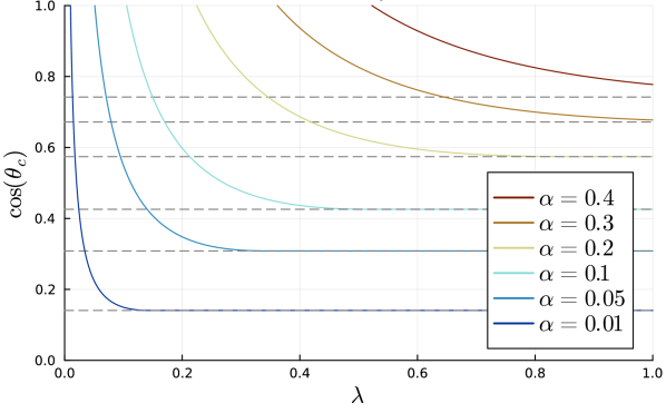
In Fig. 2 we show the critical size for the basins as discussed in Section IV. Considering a typical pattern, recovery is possible from a random initial condition on the sphere at an angle θ𝜃\theta from it as long as θ<θc(α,λ)𝜃subscript𝜃𝑐𝛼𝜆\theta<\theta_{c}(\alpha,\lambda). The expression for θcsubscript𝜃𝑐\theta_{c} is given in Appendix C. We see that the basin size decreases monotonically with α𝛼\alpha as expected. For a given α𝛼\alpha and increasing λ𝜆\lambda, we find 3 regimes: 1) No retrieval for λ<λ1(α)𝜆subscript𝜆1𝛼\lambda<\lambda_{1}(\alpha); 2) Monotonically increasing basin size for λ1(α)<λ<λ(α)subscript𝜆1𝛼𝜆subscript𝜆𝛼\lambda_{1}(\alpha)<\lambda<\lambda_{*}(\alpha); 3) Basin size frozen to θ(α)subscript𝜃𝛼\theta_{*}(\alpha) for λ>λ(α)𝜆subscript𝜆𝛼\lambda>\lambda_{*}(\alpha). The value θ(α)subscript𝜃𝛼\theta_{*}(\alpha) corresponds to the typical distance of nearest patterns. The REM is in a condensed phase in this last regime.
Refer to caption
Figure 2: Characterization of the basins of attraction given by the maximum angle θc(α,λ)subscript𝜃𝑐𝛼𝜆\theta_{c}(\alpha,\lambda) between a typical pattern and a random initialization such that the pattern is retrieved with high probability. The patterns here follow a spherical distribution and the configuration is also initialized on the hypersphere. Horizontal lines correspond to the angle of the nearest pattern.

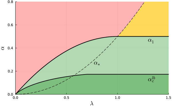
In the case of Gaussian patterns, fluctuations in the norm of the patterns lead to larger deviations from the typical behavior compared to the spherical case. The phase diagram derived in Appendix D and summarized in Fig. 3 thus differs significantly from the one of spherical patterns. The capacity threshold for typical pattern retrieval, α1(λ)subscript𝛼1𝜆\alpha_{1}(\lambda), saturates at λ=1𝜆1\lambda=1 to the value α1=1/2subscript𝛼112\alpha_{1}=1/2. The lower bound to αcsubscript𝛼𝑐\alpha_{c} no longer coincides with α1subscript𝛼1\alpha_{1}. It saturates at large λ𝜆\lambda to the value αclb=log2/ 4superscriptsubscript𝛼clb24\operatorname{\alpha_{c}^{lb}}=\log 2\,/\,4. Finally, in the region α>α1𝛼subscript𝛼1\alpha>\alpha_{1} where the patterns are not retrieved, the noise term dominating the energy, which is given by the REM term, can be either in a condensed phase or not depending on the value of λ𝜆\lambda.

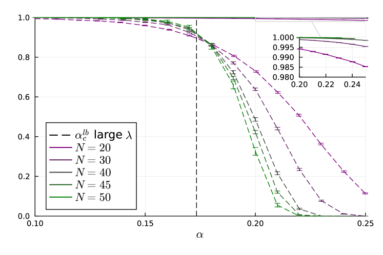
Fig. 8 of Appendix F shows that the numerical estimate of αcsubscript𝛼𝑐\alpha_{c} is close to our analytic lower bound.

Refer to caption
Figure 3: Phase diagram for Gaussian patterns, showing the critical capacity for retrieval of a typical pattern, α1subscript𝛼1\alpha_{1}, as well as the lower bound for the capacity of retrieval of all patterns, αclbsuperscriptsubscript𝛼clb\operatorname{\alpha_{c}^{lb}}. The αsubscript𝛼\alpha_{*} line is the condensation transition in the auxiliary REM. In the non-retrieval regime α>α1𝛼subscript𝛼1\alpha>\alpha_{1} there exist two phases, one with α>α𝛼subscript𝛼\alpha>\alpha_{*} where the energy is dominated by an exponential number of patterns, and the condensed phase α1<α<αsubscript𝛼1𝛼subscript𝛼\alpha_{1}<\alpha<\alpha_{*}.

VI Scaled dot-product

The dot-product found in the softmax operation of Transformer architectures is commonly scaled by a N𝑁\sqrt{N} factor [9] so that totally uncorrelated keys and queries give an O(1)𝑂1O(1) exponent. Therefore we consider a scaling regime where λ=λ~/Na𝜆~𝜆superscript𝑁𝑎\lambda=\tilde{\lambda}/N^{a} for some a(0,1)𝑎01a\in(0,1). The energy function now reads

E(𝐱)=Naλ~logμeλ~Na𝐱𝝃μ+12𝐱2.𝐸𝐱superscript𝑁𝑎~𝜆subscript𝜇superscript𝑒~𝜆superscript𝑁𝑎𝐱superscript𝝃𝜇12superscriptdelimited-∥∥𝐱2E(\operatorname{\mathbf{x}})=-\frac{N^{a}}{\tilde{\lambda}}\log\sum_{\mu}e^{\frac{\tilde{\lambda}}{N^{a}}\operatorname{\mathbf{x}}\cdot\operatorname{\bm{\xi}}^{\mu}}+\frac{1}{2}\lVert\operatorname{\mathbf{x}}\rVert^{2}. (11)

The interesting regime is now when the number of patterns scales as P=exp(α~N1a)𝑃~𝛼superscript𝑁1𝑎P=\exp(\tilde{\alpha}N^{1-a}) so that we have a competition between the noise contribution ΦΦ\Phi given by the REM and the signal term λ~Na𝝃12λ~N1a\frac{\tilde{\lambda}}{N^{a}}\rVert\operatorname{\bm{\xi}}^{1}\lVert^{2}\approx\tilde{\lambda}N^{1-a} in Eq. (3) when 𝐱=𝝃1𝐱superscript𝝃1\operatorname{\mathbf{x}}=\operatorname{\bm{\xi}}^{1}. Then, λNΦ=α~N1a𝜆𝑁Φ~𝛼superscript𝑁1𝑎\lambda N\Phi=\tilde{\alpha}N^{1-a} for any pattern ensemble. The typical pattern retrieval threshold in this setting always coincides with the all-patterns retrieval one, and they take the simple value α~1=α~c=λ~subscript~𝛼1subscript~𝛼𝑐~𝜆\tilde{\alpha}_{1}=\tilde{\alpha}_{c}=\tilde{\lambda}. In Appendix F.4 we present numerical experiments supporting this result.

VII Conclusions

Dense associative memories have exponential capacity, at the cost of using an energy function that takes an exponential number of operations. This gives a completely new regime where we can use statistical physics to determine the asymptotic memory capacity of large networks, as well as their attraction basins for zero-temperature dynamics starting from random configurations. Generalizing these results to properties of the free-energy landscape (at finite temperature), or to worst-case initial conditions is an interesting challenge: subtle effects due to the exponential number of patterns, and resulting rare events, are to be taken into account. On the other hand, it should be possible to establish rigorously our zero-temperature results and to extend them to other factorized pattern distributions, such as the case of binary patterns and continuous neurons. Finally, it would be interesting to extend the study to patterns generated from a hidden-manifold [19], and to explore implications for Transformer architectures. C.L. acknowledges funding from the European Union – Next Generation EU (MIUR PRIN 2022 and MIUR PRIN PNRR 2022).

References

  • [1] J J Hopfield. Neural networks and physical systems with emergent collective computational abilities. Proceedings of the National Academy of Sciences, 79(8):2554–2558, April 1982. Publisher: Proceedings of the National Academy of Sciences. URL: https://www.pnas.org/doi/10.1073/pnas.79.8.2554, doi:10.1073/pnas.79.8.2554.
  • [2] Daniel J Amit, Hanoch Gutfreund, and Haim Sompolinsky. Spin-glass models of neural networks. Physical Review A, 32(2):1007–1018, aug 1985. URL: http://link.aps.org/doi/10.1103/PhysRevA.32.1007, doi:10.1103/PhysRevA.32.1007.
  • [3] Daniel J. Amit, Hanoch Gutfreund, and Haim Sompolinsky. Storing Infinite Numbers of Patterns in a Spin-Glass Model of Neural Networks. Physical Review Letters, 55(14):1530–1533, sep 1985. URL: https://link.aps.org/doi/10.1103/PhysRevLett.55.1530, doi:10.1103/PhysRevLett.55.1530.
  • [4] E. Gardner. Multiconnected neural network models. Journal of Physics A: Mathematical and General, 20(11):3453–3464, August 1987. URL: https://iopscience.iop.org/article/10.1088/0305-4470/20/11/046, doi:10.1088/0305-4470/20/11/046.
  • [5] Dmitry Krotov and John J. Hopfield. Dense associative memory for pattern recognition. Advances in Neural Information Processing Systems, pages 1180–1188, 2016. URL: http://arxiv.org/abs/1606.01164.
  • [6] Elena Agliari, Linda Albanese, Francesco Alemanno, Andrea Alessandrelli, Adriano Barra, Fosca Giannotti, Daniele Lotito, and Dino Pedreschi. Dense hebbian neural networks: A replica symmetric picture of supervised learning. Physica A: Statistical Mechanics and its Applications, 626:129076, 2023. URL: https://www.sciencedirect.com/science/article/pii/S0378437123006313, doi:10.1016/j.physa.2023.129076.
  • [7] Mete Demircigil, Judith Heusel, Matthias Löwe, Sven Upgang, and Franck Vermet. On a Model of Associative Memory with Huge Storage Capacity. Journal of Statistical Physics, 168(2):288–299, July 2017. arXiv: 1702.01929. URL: http://arxiv.org/abs/1702.01929, doi:10.1007/s10955-017-1806-y.
  • [8] Hubert Ramsauer, Bernhard Schäfl, Johannes Lehner, Philipp Seidl, Michael Widrich, Lukas Gruber, Markus Holzleitner, Thomas Adler, David Kreil, Michael K Kopp, Günter Klambauer, Johannes Brandstetter, and Sepp Hochreiter. Hopfield networks is all you need. In International Conference on Learning Representations, 2021. URL: https://openreview.net/forum?id=tL89RnzIiCd.
  • [9] Ashish Vaswani, Noam Shazeer, Niki Parmar, Jakob Uszkoreit, Llion Jones, Aidan N Gomez, Łukasz Kaiser, and Illia Polosukhin. Attention is all you need. In Advances in neural information processing systems, pages 5998–6008, 2017.
  • [10] Dzmitry Bahdanau, Kyunghyun Cho, and Yoshua Bengio. Neural machine translation by jointly learning to align and translate. In Yoshua Bengio and Yann LeCun, editors, 3rd International Conference on Learning Representations, ICLR 2015, San Diego, CA, USA, May 7-9, 2015, Conference Track Proceedings, 2015. URL: http://arxiv.org/abs/1409.0473.
  • [11] Anton Bovier. Sharp upper bounds on perfect retrieval in the hopfield model. Journal of Applied Probability, 36(3):941–950, 1999. URL: http://www.jstor.org/stable/3215454.
  • [12] Bernard Derrida. Random-energy model: An exactly solvable model of disordered systems. Physical Review B, 24(5):2613–2626, sep 1981. URL: http://link.aps.org/doi/10.1103/PhysRevB.24.2613https://link.aps.org/doi/10.1103/PhysRevB.24.2613, doi:10.1103/PhysRevB.24.2613.
  • [13] Daniel J. Amit, Hanoch Gutfreund, and Haim Sompolinsky. Statistical mechanics of neural networks near saturation. Annals of Physics, 173(1):30–67, January 1987. URL: https://linkinghub.elsevier.com/retrieve/pii/0003491687900923.
  • [14] M. Fedrigo, F. Flandoli, and F. Morandin. A Large Deviation Principle for the free energy of random Gibbs measures with application to the REM. Annali di Matematica Pura ed Applicata, 186(3):381–417, July 2007. doi:10.1007/s10231-006-0011-4.
  • [15] E. Gardner and B. Derrida. The probability distribution of the partition function of the random energy model. Journal of Physics A: Mathematical and General, 22(12):1975, June 1989. URL: https://dx.doi.org/10.1088/0305-4470/22/12/003, doi:10.1088/0305-4470/22/12/003.
  • [16] Marc Mézard and Andrea Montanari. Information, physics, and computation. Oxford Univ. Press, 2009.
  • [17] Tom Richardson and Rüdiger Urbanke. Modern Coding Theory. Cambridge University Press, 2008.
  • [18] Elena Agliari, Francesco Alemanno, Adriano Barra, Martino Centonze, and Alberto Fachechi. Neural networks with a redundant representation: Detecting the undetectable. Phys. Rev. Lett., 124:028301, Jan 2020. URL: https://link.aps.org/doi/10.1103/PhysRevLett.124.028301, doi:10.1103/PhysRevLett.124.028301.
  • [19] M. Negri, C. Lauditi, G. Perugini, C. Lucibello, and E. Malatesta. Storage and learning phase transitions in the random-features hopfield model. Phys. Rev. Lett., 131:257301, Dec 2023. URL: https://link.aps.org/doi/10.1103/PhysRevLett.131.257301, doi:10.1103/PhysRevLett.131.257301.
  • [20] David Ruelle. A mathematical reformulation of derrida’s rem and grem. Communications in Mathematical Physics, 108:225–239, 1987.
  • [21] Anton Bovier, Irina Kurkova, and Matthias Löwe. Fluctuations of the free energy in the rem and the p𝑝p-spin sk models. The Annals of Probability, 30(2):605–651, 2002.
  • [22] Jean-Philippe Bouchaud and Marc Mézard. Universality classes for extreme-value statistics. Journal of Physics A: Mathematical and General, 30(23):7997, dec 1997. URL: https://dx.doi.org/10.1088/0305-4470/30/23/004, doi:10.1088/0305-4470/30/23/004.
  • [23] Marc Mézard, Giorgio Parisi, and Miguel Angel Virasoro. Spin glass theory and beyond: An Introduction to the Replica Method and Its Applications, volume 9. World Scientific Publishing Company, 1987.
  • [24] Mauro Pastore. Replicas in complex systems: applications to large deviations and neural networks. PhD thesis, 2021.

Appendix A Computation of the noise function Φ(x)Φ𝑥\Phi(x)

This Appendix aims to present in a self-contained way the Random Energy Model (REM) analysis which is used to derive the noise function Φ(𝐱)Φ𝐱\Phi(\operatorname{\mathbf{x}}). This analysis uses the methods that were initially developed by Derrida [12], and generalizes them to a broader range of problems, including the ones which are encountered when computing Φ(𝐱)Φ𝐱\Phi(\operatorname{\mathbf{x}}). In the more than 40 years since Derrida’s work, numerous papers have appeared on the REM, its mathematical formalism [20, 21], and its generalizations [22]. The present Appendix cannot give a fair account of all these developments, therefore it will present the main ideas without going into the details of mathematical proofs, but we hope that it will give a reasonably self-contained set of ideas and methods for colleagues who are not experts in statistical physics of disordered systems. The Chapter 5 of [16] also provides a self-contained introduction to the REM itself. We mainly follow here the line of approach of that chapter, extending it to the more general setup useful for our present problem. This Appendix is divided into four subsections. Section A.1 gives the general analysis of partition functions of a REM type, when the statistics of the random variables is known. Section A.2 studies the statistics of the random variables that appear in the noise Φ(𝐱)Φ𝐱\Phi(\operatorname{\mathbf{x}}) in dense associative memories. Section A.3 summarizes the various steps of the derivation of the noise function. Section A.4 presents an alternative approach to the computation of Φ(𝐱)Φ𝐱\Phi(\operatorname{\mathbf{x}}) using replicas: it gives back the same results as the direct approach of the first three subsections, in a more compact way. Although this is neither particularly transparent nor rigorous, we include it here because it is an interesting approach in itself and it also gives a path towards studying large deviations.

A.1 REM partition functions

Consider a set 𝒮𝒮{\mathcal{S}} of P=eαN𝑃superscript𝑒𝛼𝑁P=e^{\alpha N} independent random variables εμsuperscript𝜀𝜇\varepsilon^{\mu} which are i.i.d. random variables with probability density function (pdf) pN(ε)subscript𝑝𝑁𝜀p_{N}(\varepsilon). The pdf is assumed to satisfy, at large N𝑁N, a large deviation principle with a certain rate function s(ε)𝑠𝜀s({\varepsilon}). That is, for large N𝑁N and any a<b𝑎𝑏a<b we have, at the leading exponential order we have

ab𝑑εpN(ε)eNmaxε[a,b]s(ε).superscriptsubscript𝑎𝑏differential-d𝜀subscript𝑝𝑁𝜀superscript𝑒𝑁subscript𝜀𝑎𝑏𝑠𝜀\displaystyle\int_{a}^{b}d{\varepsilon}\;p_{N}(\varepsilon)\approx e^{-N\max_{{\varepsilon}\in[a,b]}s({\varepsilon})}. (12)

A classical choice [12] for the pdf is pN=𝒩(0,1/N)subscript𝑝𝑁𝒩01𝑁p_{N}=\mathcal{N}(0,1/N). In the cases that we shall study, the function s(ε)𝑠𝜀s({\varepsilon}) is a convex non-negative function, which vanishes at the typical value of the random variable. In the usual REM, the independent random variables εμsuperscript𝜀𝜇{\varepsilon}^{\mu} are called energies, hence the name of the model. The energies in the auxiliary REM model are not to be confused with the main object of our study, the energy function E(𝐱)𝐸𝐱E(\operatorname{\mathbf{x}}) of the dense associative memory in Eq. (1). The REM partition function is defined as

Z=μ=1PeλNεμ.𝑍superscriptsubscript𝜇1𝑃superscript𝑒𝜆𝑁superscript𝜀𝜇\displaystyle Z=\sum_{\mu=1}^{P}e^{\lambda N{\varepsilon}^{\mu}}\ . (13)

Notice that at odds with the usual statistical physics definition, the energies appear in the exponent with a plus sign instead of a minus. It depends on a parameter λ𝜆\lambda that we choose positive without loss of generality. It plays the role of an inverse temperature: increasing λ𝜆\lambda, the εμsuperscript𝜀𝜇{\varepsilon}^{\mu} with higher values will give the dominant contribution to Z𝑍Z. One can define the free-energy density of the REM as Φ=1λNlogZΦ1𝜆𝑁𝑍\Phi=\frac{1}{\lambda N}\log Z. A main consequence of the independence of the variables in 𝒮𝒮{\mathcal{S}}, and of the specific large-deviation form of their distribution is that, in the large N𝑁N limit, the random variable ΦΦ\Phi concentrates: its distribution becomes peaked around its typical value

ϕα(λ)=limN𝔼Φ,subscriptitalic-ϕ𝛼𝜆subscript𝑁𝔼Φ\phi_{\alpha}(\lambda)=\lim_{N\to\infty}\mathbb{E}\,\Phi, (14)

with a standard deviation that goes to zero as 1/N1𝑁1/\sqrt{N}. Let us see how one can compute the typical value of the free energy density in the large N𝑁N limit, ϕitalic-ϕ\phi, which depends on α,λ𝛼𝜆\alpha,\lambda and on the rate function s(ε)𝑠𝜀s({\varepsilon}), and justify the concentration property. In the large N𝑁N limit, let us call 𝒩[a,b]subscript𝒩𝑎𝑏\mathcal{N}_{[a,b]} the number of random variables of 𝒮𝒮{\mathcal{S}} (among the P=eαN𝑃superscript𝑒𝛼𝑁P=e^{\alpha N} it contains) which are in the interval [a,b]𝑎𝑏[a,b]. Its expected value is

𝔼𝒩[a,b]=eN(αmaxε[a,b]s(ε)),𝔼subscript𝒩𝑎𝑏superscript𝑒𝑁𝛼subscript𝜀𝑎𝑏𝑠𝜀\displaystyle\mathbb{E}\,\mathcal{N}_{[a,b]}=e^{N(\alpha-\max_{{\varepsilon}\in[a,b]}s({\varepsilon}))}, (15)

therefore the average density of random variables around ε𝜀{\varepsilon} is eN(αs(ε))superscript𝑒𝑁𝛼𝑠𝜀e^{N(\alpha-s({\varepsilon}))}. The function αs(ε)𝛼𝑠𝜀\alpha-s({\varepsilon}) is a concave function of ε𝜀{\varepsilon}, it vanishes for certain values ε=εm(α)𝜀subscript𝜀𝑚𝛼{\varepsilon}={\varepsilon}_{m}(\alpha) and ε=ε(α)𝜀subscript𝜀𝛼{\varepsilon}={\varepsilon}_{*}(\alpha), with εm(α)<ε0<ε(α)subscript𝜀𝑚𝛼subscript𝜀0subscript𝜀𝛼{\varepsilon}_{m}(\alpha)<{\varepsilon}_{0}<{\varepsilon}_{*}(\alpha), it is positive for ε[εm(α),ε(α)]𝜀subscript𝜀𝑚𝛼subscript𝜀𝛼{\varepsilon}\in[{\varepsilon}_{m}(\alpha),\,{\varepsilon}_{*}(\alpha)] and it is negative outside of this interval. Using the first- and second-moment methods, one can prove that at large N𝑁N, 1Nlog𝒩[a,b]1𝑁subscript𝒩𝑎𝑏\frac{1}{N}\log\mathcal{N}_{[a,b]} concentrates around maxε[a,b]ψα(ε)subscript𝜀𝑎𝑏subscript𝜓𝛼𝜀\max_{{\varepsilon}\in[a,b]}\psi_{\alpha}({\varepsilon}), where:

ψα(ε)={αs(ε)if ε[εm(α),ε(α)]otherwisesubscript𝜓𝛼𝜀cases𝛼𝑠𝜀if 𝜀subscript𝜀𝑚𝛼subscript𝜀𝛼otherwise\psi_{\alpha}({\varepsilon})=\begin{cases}\alpha-s({\varepsilon})&\text{if }{\varepsilon}\in[{\varepsilon}_{m}(\alpha),\,{\varepsilon}_{*}(\alpha)]\\ -\infty&\text{otherwise}\end{cases} (16)

We shall not detail this proof, referring the reader to [12]. Let us just mention the ideas behind the proofs. The first moment method uses Jensen’s inequality log𝔼𝒩[a,b]𝔼log𝒩[a,b]𝔼subscript𝒩𝑎𝑏𝔼subscript𝒩𝑎𝑏\log\mathbb{E}\mathcal{N}_{[a,b]}\geq\mathbb{E}\log\mathcal{N}_{[a,b]} in order to show that, when αs(ε)<0𝛼𝑠𝜀0\alpha-s({\varepsilon})<0, the average number of variables in 𝒮𝒮{\mathcal{S}} around ε𝜀{\varepsilon} is exponentially small in N𝑁N, which implies that the typical number of energies is zero. This explains the -\infty case in Eq. (16). The second moment method uses the independence of the variables to show that, when 𝔼𝒩[a,b]𝔼subscript𝒩𝑎𝑏\mathbb{E}\mathcal{N}_{[a,b]} is exponentially large in N𝑁N, the relative fluctuations 𝔼(𝒩[a,b]2)(𝔼𝒩[a,b])2/(𝔼𝒩[a,b])𝔼superscriptsubscript𝒩𝑎𝑏2superscript𝔼subscript𝒩𝑎𝑏2𝔼subscript𝒩𝑎𝑏\sqrt{\mathbb{E}(\mathcal{N}_{[a,b]}^{2})-(\mathbb{E}\mathcal{N}_{[a,b]})^{2}}/(\mathbb{E}\mathcal{N}_{[a,b]}) are exponentially small, leading to the concentration result (16).

Let us study the partition function (13). Using the concentration property for the density of levels (16), one obtains the large N𝑁N behaviour

Zεm(α)ε(α)𝑑εeN(αs(ε)+λε).𝑍superscriptsubscriptsubscript𝜀𝑚𝛼subscript𝜀𝛼differential-d𝜀superscript𝑒𝑁𝛼𝑠𝜀𝜆𝜀\displaystyle Z\approx\int_{{\varepsilon}_{m}(\alpha)}^{{\varepsilon}_{*}(\alpha)}d{\varepsilon}\;e^{N(\alpha-s({\varepsilon})+\lambda{\varepsilon})}. (17)

This integral can be evaluated using Laplace’s method which gives

limN1NlogZ=maxε[εm(α),ε(α)]αs(ε)+λε,subscript𝑁1𝑁𝑍subscript𝜀subscript𝜀𝑚𝛼subscript𝜀𝛼𝛼𝑠𝜀𝜆𝜀\displaystyle\lim_{N\to\infty}\frac{1}{N}\log Z=\max_{{\varepsilon}\in[{\varepsilon}_{m}(\alpha),\,{\varepsilon}_{*}(\alpha)]}\ \alpha-s({\varepsilon})+\lambda{\varepsilon}, (18)

where equality is in the sense of almost sure convergence. Depending on the value of λ>0𝜆0\lambda>0, we find two regimes separated by a critical value λ(α)=s(ε(α))subscript𝜆𝛼superscript𝑠subscript𝜀𝛼\lambda_{*}(\alpha)=s^{\prime}({\varepsilon}_{*}(\alpha)). If λ<λ(α)𝜆subscript𝜆𝛼\lambda<\lambda_{*}(\alpha), the maximum is found at a value ε=ε~(λ)𝜀~𝜀𝜆{\varepsilon}=\tilde{{\varepsilon}}(\lambda), with εm(α)<ε~<ε(α)subscript𝜀𝑚𝛼~𝜀subscript𝜀𝛼{\varepsilon}_{m}(\alpha)<\tilde{{\varepsilon}}<{\varepsilon}_{*}(\alpha), obtained as the stationary point of αs(ε)+λε𝛼𝑠𝜀𝜆𝜀\alpha-s({\varepsilon})+\lambda{\varepsilon}. In this regime, an exponentially large number of variables εμsuperscript𝜀𝜇{\varepsilon}^{\mu} contribute to the partition function (the entropy of the REM is proportional to N𝑁N). On the contrary when λλ(α)𝜆subscript𝜆𝛼\lambda\geq\lambda_{*}(\alpha), the maximum is at ε(α)subscript𝜀𝛼{\varepsilon}_{*}(\alpha) and the entropy vanishes. The transition between these two regimes is called condensation transition.

This discussion leads to the following result: the free-energy density of a REM-type model, 1λNlogZ1𝜆𝑁𝑍\frac{1}{\lambda N}\log Z, concentrates at large N𝑁N to the value

ϕα(λ)subscriptitalic-ϕ𝛼𝜆\displaystyle\phi_{\alpha}(\lambda) ={ε~(λ)+αs(ε~(λ))λλ<λ(α)ε(α)λλ(α)absentcases~𝜀𝜆𝛼𝑠~𝜀𝜆𝜆𝜆subscript𝜆𝛼subscript𝜀𝛼𝜆subscript𝜆𝛼\displaystyle=\begin{cases}\tilde{{\varepsilon}}(\lambda)+\frac{\alpha-s(\tilde{{\varepsilon}}(\lambda))}{\lambda}&\lambda<\lambda_{*}(\alpha)\\ {\varepsilon}_{*}(\alpha)&\lambda\geq\lambda_{*}(\alpha)\end{cases} (19)

where ε~(λ)~𝜀𝜆\tilde{{\varepsilon}}(\lambda) is defined by λ=s(ε~)𝜆superscript𝑠~𝜀\lambda=s^{\prime}(\tilde{{\varepsilon}}), The critical value λ(α)subscript𝜆𝛼\lambda_{*}(\alpha) instead is found when ε(λ)𝜀𝜆{\varepsilon}(\lambda) becomes equal to the maximal value ε(α)subscript𝜀𝛼{\varepsilon}_{*}(\alpha) of the P=eαN𝑃superscript𝑒𝛼𝑁P=e^{\alpha N} random variables: λ(α)=s(ε(α))subscript𝜆𝛼superscript𝑠subscript𝜀𝛼\lambda_{*}(\alpha)=s^{\prime}({\varepsilon}_{*}(\alpha)).

In the next sections, we discuss how to compute the rate function s(ε)𝑠𝜀s({\varepsilon}) and summarize the steps needed to apply the formalism to our original dense associative memory problem.

A.2 Determination of the rate function

Let us go back to the definition (4)italic-(4italic-)\eqref{eq:def-Phi} of the noise term in our analysis of the dense associative memory in presence of P=eαN𝑃superscript𝑒𝛼𝑁P=e^{\alpha N} memories 𝝃μNsuperscript𝝃𝜇superscript𝑁\operatorname{\bm{\xi}}^{\mu}\in\mathbb{R}^{N} independently sampled from a density function pN(𝝃)subscript𝑝𝑁𝝃p_{N}(\operatorname{\bm{\xi}}):

Φ(𝐱)=1Nλlog(μ=2Peλ𝐱𝝃μ).Φ𝐱1𝑁𝜆superscriptsubscript𝜇2𝑃superscript𝑒𝜆𝐱superscript𝝃𝜇\displaystyle\Phi(\operatorname{\mathbf{x}})=\frac{1}{N\lambda}\log\left(\sum_{\mu=2}^{P}e^{\lambda\operatorname{\mathbf{x}}\cdot\operatorname{\bm{\xi}}^{\mu}}\right). (20)

We consider the vector 𝐱𝐱\operatorname{\mathbf{x}}, chosen independently from patterns {𝝃μ}μ=2,,Psubscriptsuperscript𝝃𝜇𝜇2𝑃\{\operatorname{\bm{\xi}}^{\mu}\}_{\mu=2,...,P}. We are in a situation similar to the REM partition function of Eq. (13)italic-(13italic-)\eqref{REMdef}, where the i.i.d. random variables are εμ=1N𝐱𝝃μsuperscript𝜀𝜇1𝑁𝐱superscript𝝃𝜇{\varepsilon}^{\mu}=\frac{1}{N}\operatorname{\mathbf{x}}\cdot\operatorname{\bm{\xi}}^{\mu}. We need to establish that the large deviation principle (12)italic-(12italic-)\eqref{eq:rate-s} applies and compute the rate function s(ε)𝑠𝜀s({\varepsilon}).

We introduce the generating function:

Γ(λ,𝐱)=d𝝃pN(𝝃)eλ𝐱𝝃Γ𝜆𝐱𝑑𝝃subscript𝑝𝑁𝝃superscript𝑒𝜆𝐱𝝃\displaystyle\Gamma(\lambda,\operatorname{\mathbf{x}})=\int d\operatorname{\bm{\xi}}p_{N}(\operatorname{\bm{\xi}})\,e^{\lambda\operatorname{\mathbf{x}}\cdot\operatorname{\bm{\xi}}} (21)

Where the expectation is over the pattern distribution pN𝝃)p_{N}\operatorname{\bm{\xi}}). A priori, this generating function depends on the full vector 𝐱𝐱\operatorname{\mathbf{x}}. Assuming that the distribution pN(𝝃)subscript𝑝𝑁𝝃p_{N}(\operatorname{\bm{\xi}}) is rotationally invariant, one finds that ζ𝐱subscript𝜁𝐱\zeta_{\operatorname{\mathbf{x}}} depends on 𝐱𝐱\operatorname{\mathbf{x}} only through its norm, 𝐱=ρN𝐱𝜌𝑁\operatorname{\mathbf{x}}=\rho\sqrt{N}. We also assume that ΓΓ\Gamma satisfies a large deviation principle with a (negative) rate function ζρ(λ)subscript𝜁𝜌𝜆\zeta_{\rho}(\lambda) , that is for large N𝑁N we have

Γ(λ,𝐱)eNζρ(λ)Γ𝜆𝐱superscript𝑒𝑁subscript𝜁𝜌𝜆\displaystyle\Gamma(\lambda,\operatorname{\mathbf{x}})\approx e^{N\zeta_{\rho}(\lambda)}\ (22)

Under the assumptions of Gärtner-Ellis theorem, this implies that the distribution ρN(ε)subscript𝜌𝑁𝜀\rho_{N}({\varepsilon}) satisfies a large deviation principle with a rate function sρ(ε)subscript𝑠𝜌𝜀s_{\rho}({\varepsilon}), which is the Legendre transform of ζρ(λ)subscript𝜁𝜌𝜆\zeta_{\rho}(\lambda). In fact, writing

Γ(u,𝐱)𝑑εeNsρ(ε)eλNεeNζρ(u),Γ𝑢𝐱differential-d𝜀superscript𝑒𝑁subscript𝑠𝜌𝜀superscript𝑒𝜆𝑁𝜀superscript𝑒𝑁subscript𝜁𝜌𝑢\displaystyle\Gamma(u,\operatorname{\mathbf{x}})\approx\int d{\varepsilon}\ e^{-Ns_{\rho}({\varepsilon})}e^{\lambda N{\varepsilon}}\approx e^{N\zeta_{\rho}(u)}, (23)

we find the relations

ζρ(λ)=supελεsρ(ε)subscript𝜁𝜌𝜆subscriptsupremum𝜀𝜆𝜀subscript𝑠𝜌𝜀\displaystyle\zeta_{\rho}(\lambda)=\sup_{\varepsilon}\ \lambda{\varepsilon}-s_{\rho}({\varepsilon}) (24)

and

sρ(ε)=supλλεζρ(λ).subscript𝑠𝜌𝜀subscriptsupremum𝜆𝜆𝜀subscript𝜁𝜌𝜆\displaystyle s_{\rho}({\varepsilon})=\sup_{\lambda}\ \lambda{\varepsilon}-\zeta_{\rho}(\lambda). (25)

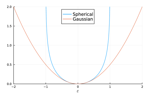
The rate function sρ(ε)subscript𝑠𝜌𝜀s_{\rho}({\varepsilon}) is shown in Fig. 4 for the Gaussian and Spherical pattern ensembles.
Refer to caption
Figure 4: The REM rate function sρ(ε)subscript𝑠𝜌𝜀s_{\rho}({\varepsilon}) for ρ=1𝜌1\rho=1 and the two pattern ensembles considered in this paper.

A.3 Summary of the noise function computation

We summarize here the general approach for finding the large N𝑁N limit of the REM-like noise term Φ(𝐱)Φ𝐱\Phi(\operatorname{\mathbf{x}}) in (4), with P=eαN𝑃superscript𝑒𝛼𝑁P=e^{\alpha N} patterns independently sampled from a rotationally invariant distribution pN(𝝃)subscript𝑝𝑁𝝃p_{N}(\operatorname{\bm{\xi}}).

For increasing N𝑁N, we consider a sequence of vectors 𝐱N𝐱superscript𝑁\operatorname{\mathbf{x}}\in\mathbb{R}^{N} and patterns 𝝃μNsuperscript𝝃𝜇superscript𝑁\operatorname{\bm{\xi}}^{\mu}\in\mathbb{R}^{N}, such that 𝐱𝐱\operatorname{\mathbf{x}} is chosen independently from {𝝃μ}μ=2,,Psubscriptsuperscript𝝃𝜇𝜇2𝑃\{\operatorname{\bm{\xi}}^{\mu}\}_{\mu=2,...,P} and with norm 𝐱=ρNdelimited-∥∥𝐱𝜌𝑁\lVert\operatorname{\mathbf{x}}\rVert=\rho\sqrt{N}. Thanks to rotational invariance and to concentration of the REM free energy on its expected value (the self-averaging property in statistical physics jargon), we have

ϕα,ρ(λ)=limN1NΦ(𝐱).subscriptitalic-ϕ𝛼𝜌𝜆subscript𝑁1𝑁Φ𝐱\phi_{\alpha,\rho}(\lambda)=\lim_{N\to\infty}\frac{1}{N}\Phi(\operatorname{\mathbf{x}}). (26)

The asymptotic value ϕρ(λ)subscriptitalic-ϕ𝜌𝜆\phi_{\rho}(\lambda) is thus obtained as follows:

  1. 1.

    Find the generating function ζρ(λ)subscript𝜁𝜌𝜆\zeta_{\rho}(\lambda) defined in (22):

    ζρ(λ)=limN+1Nlog𝔼𝝃eλ𝐱𝝃.subscript𝜁𝜌𝜆subscript𝑁1𝑁subscript𝔼𝝃superscript𝑒𝜆𝐱𝝃\zeta_{\rho}(\lambda)=\lim_{N\to+\infty}\frac{1}{N}\log\mathbb{E}_{\operatorname{\bm{\xi}}}\,e^{\lambda\operatorname{\mathbf{x}}\cdot\operatorname{\bm{\xi}}}. (27)
  2. 2.

    Using the Legendre transform (25), find the rate function sρ(ε)=supλλεζρ(λ)subscript𝑠𝜌𝜀subscriptsupremum𝜆𝜆𝜀subscript𝜁𝜌𝜆s_{\rho}({\varepsilon})=\sup_{\lambda}\ \lambda{\varepsilon}-\zeta_{\rho}(\lambda).

  3. 3.

    For a given value of α𝛼\alpha, find the values εm(α,ρ)<ε(α,ρ)subscript𝜀𝑚𝛼𝜌subscript𝜀𝛼𝜌{\varepsilon}_{m}(\alpha,\rho)<{\varepsilon}_{*}(\alpha,\rho) which are the two solutions of αsρ(ε)=0𝛼subscript𝑠𝜌𝜀0\alpha-s_{\rho}({\varepsilon})=0. We are assuming here sρ(ε)subscript𝑠𝜌𝜀s_{\rho}({\varepsilon}) to be concave and unbounded above. For bounded sρ(ε)subscript𝑠𝜌𝜀s_{\rho}({\varepsilon}), the argument has to be slightly modified.

  4. 4.

    Obtain the condensation threshold λ(α,ρ)=sρ(ε(α,ρ))subscript𝜆𝛼𝜌superscriptsubscript𝑠𝜌subscript𝜀𝛼𝜌\lambda_{*}(\alpha,\rho)=s_{\rho}^{\prime}({\varepsilon}_{*}(\alpha,\rho)).

  5. 5.

    Obtain the energy level ε~(λ,ρ)~𝜀𝜆𝜌\tilde{\varepsilon}(\lambda,\rho) dominating the uncondensed phase as the stationary point of λεsρ(ε)𝜆𝜀subscript𝑠𝜌𝜀\lambda{\varepsilon}-s_{\rho}({\varepsilon}).

  6. 6.

    Finally compute ϕα,ρ(λ)subscriptitalic-ϕ𝛼𝜌𝜆\phi_{\alpha,\rho}(\lambda) as

    ϕα,ρ(λ)={ε~(λ,ρ)+αsρ(ε~(λ,ρ))λ=α+ζρ(λ)λλ<λ(α,ρ)ε(α,ρ)λλ(α,ρ).subscriptitalic-ϕ𝛼𝜌𝜆cases~𝜀𝜆𝜌𝛼subscript𝑠𝜌~𝜀𝜆𝜌𝜆𝛼subscript𝜁𝜌𝜆𝜆𝜆subscript𝜆𝛼𝜌subscript𝜀𝛼𝜌𝜆subscript𝜆𝛼𝜌\displaystyle\phi_{\alpha,\rho}(\lambda)=\begin{cases}\tilde{{\varepsilon}}(\lambda,\rho)+\frac{\alpha-s_{\rho}(\tilde{{\varepsilon}}(\lambda,\rho))}{\lambda}=\frac{\alpha+\zeta_{\rho}(\lambda)}{\lambda}&\lambda<\lambda_{*}(\alpha,\rho)\\ {\varepsilon}_{*}(\alpha,\rho)&\lambda\geq\lambda_{*}(\alpha,\rho).\end{cases} (28)

A.4 An alternative approach: replicas

We now show how to obtain the same result for the free energy using the replica method, generalizing the derivation in Refs. [12, 16]. It is convenient to use rotational invariance and rewrite the free energy as

ϕα,ρ(λ)=limN1λN𝔼logμ=2PeλρNξ1μ.subscriptitalic-ϕ𝛼𝜌𝜆subscript𝑁1𝜆𝑁𝔼superscriptsubscript𝜇2𝑃superscript𝑒𝜆𝜌𝑁superscriptsubscript𝜉1𝜇\phi_{\alpha,\rho}(\lambda)=\lim_{N\to\infty}\frac{1}{\lambda N}\mathbb{E}\log\sum_{\mu=2}^{P}e^{\lambda\rho\sqrt{N}\xi_{1}^{\mu}}. (29)

It is clear that the ρ𝜌\rho dependence could be reabsorbed in the λ𝜆\lambda one (or vice-versa), but we will keep both parameters for consistency with the main discussion. We then consider an integer number n>0𝑛0n>0 of replicas, with n𝑛n to be sent to zero by analytical continuation at the end of the computation. The average replicated partition function reads

𝔼Zn𝔼superscript𝑍𝑛\displaystyle\mathbb{E}\,Z^{n} =𝔼μ1,,μneλρNa=1nξ1μa.absent𝔼subscriptsubscript𝜇1subscript𝜇𝑛superscript𝑒𝜆𝜌𝑁superscriptsubscript𝑎1𝑛superscriptsubscript𝜉1subscript𝜇𝑎\displaystyle=\mathbb{E}\sum_{\mu_{1},\dots,\mu_{n}}e^{\lambda\rho\sqrt{N}\sum_{a=1}^{n}\xi_{1}^{\mu_{a}}}. (30)

In order to decouple the average over patterns, we introduce the variables mμsubscript𝑚𝜇m_{\mu} defined by mμ=a=1nδμa,μsubscript𝑚𝜇superscriptsubscript𝑎1𝑛subscript𝛿subscript𝜇𝑎𝜇m_{\mu}=\sum_{a=1}^{n}\delta_{\mu_{a},\mu} for a given choice of the labels μasubscript𝜇𝑎\mu_{a}. Defining the combinatorial factor

M({mμ}μ)={μa}aμδ(mμaδμa,μ),𝑀subscriptsubscript𝑚𝜇𝜇subscriptsubscriptsubscript𝜇𝑎𝑎subscriptproduct𝜇𝛿subscript𝑚𝜇subscript𝑎subscript𝛿subscript𝜇𝑎𝜇M(\{m_{\mu}\}_{\mu})=\sum_{\{\mu_{a}\}_{a}}\prod_{\mu}\delta(m_{\mu}-\sum_{a}\delta_{\mu_{a},\mu}), (31)

we obtain

𝔼Zn𝔼superscript𝑍𝑛\displaystyle\mathbb{E}\,Z^{n} =𝔼{nμ}μM({mμ}μ)eμmμρNξ1μabsent𝔼subscriptsubscriptsubscript𝑛𝜇𝜇𝑀subscriptsubscript𝑚𝜇𝜇superscript𝑒subscript𝜇subscript𝑚𝜇𝜌𝑁superscriptsubscript𝜉1𝜇\displaystyle=\mathbb{E}\sum_{\{n_{\mu}\}_{\mu}}M(\{m_{\mu}\}_{\mu})\ e^{\sum_{\mu}m_{\mu}\rho\sqrt{N}\xi_{1}^{\mu}} (32)
={mμ}μM({mμ}μ)eNμζρ(λmμ),absentsubscriptsubscriptsubscript𝑚𝜇𝜇𝑀subscriptsubscript𝑚𝜇𝜇superscript𝑒𝑁subscript𝜇subscript𝜁𝜌𝜆subscript𝑚𝜇\displaystyle=\sum_{\{m_{\mu}\}_{\mu}}M(\{m_{\mu}\}_{\mu})\ e^{N\sum_{\mu}\zeta_{\rho}(\lambda m_{\mu})}, (33)

where ζρ(λ)subscript𝜁𝜌𝜆\zeta_{\rho}(\lambda) is the generating function given by the single pattern expectation

ζρ(λ)=limN1Nlog𝔼𝝃eNλρξ1.subscript𝜁𝜌𝜆subscript𝑁1𝑁subscript𝔼𝝃superscript𝑒𝑁𝜆𝜌subscript𝜉1\zeta_{\rho}(\lambda)=\lim_{N\to\infty}\frac{1}{N}\log\mathbb{E}_{\operatorname{\bm{\xi}}}\,e^{\sqrt{N}\lambda\rho\xi_{1}}. (34)

Notice that this is the same ζρ(λ)subscript𝜁𝜌𝜆\zeta_{\rho}(\lambda) of Eqs. (24) and (27). We will now make an ansatz corresponding to one step of replica symmetry breaking (1RSB) [23, 16] for the values of mμsubscript𝑚𝜇m_{\mu} dominating the summation.

1RSB ansatz: The n𝑛n replicas μasubscript𝜇𝑎\mu_{a} are divided into n/m𝑛𝑚n/m groups of size m𝑚m. Within a group, all μasubscript𝜇𝑎\mu_{a} are the same. Different groups have different μasubscript𝜇𝑎\mu_{a}. Therefore mμ=msubscript𝑚𝜇𝑚m_{\mu}=m for nm𝑛𝑚\frac{n}{m} of the patterns, and mμ=0subscript𝑚𝜇0m_{\mu}=0 for the others.

The parameter m𝑚m, which has to be optimized, is called the Parisi 1RSB parameter. Within this ansatz, we have M=enαmN𝑀superscript𝑒𝑛𝛼𝑚𝑁M=e^{n\frac{\alpha}{m}N}, from which one obtains

ϕα,ρ(λ)=1λinfm[0,1][αm+1mζρ(λm)].subscriptitalic-ϕ𝛼𝜌𝜆1𝜆subscriptinfimum𝑚01delimited-[]𝛼𝑚1𝑚subscript𝜁𝜌𝜆𝑚\phi_{\alpha,\rho}(\lambda)=\frac{1}{\lambda}\,\inf_{m\in[0,1]}\ \left[\frac{\alpha}{m}+\frac{1}{m}\zeta_{\rho}(\lambda m)\right]\ . (35)

For any given ρ𝜌\rho, the optimal value for the Parisi parameter m𝑚m is increasing in α𝛼\alpha. Moreover, we also assume the monotonicity of ζρ(λ)subscript𝜁𝜌𝜆\zeta_{\rho}(\lambda), which implies that the optimal m𝑚m is monotonous in λ𝜆\lambda as well. We now define as m(α,ρ,λ)subscript𝑚𝛼𝜌𝜆m_{*}(\alpha,\rho,\lambda) the value of m𝑚m obtained imposing a stationarity condition in Eq. (35):

αm21m2ζρ(λm)+λmζρ(λm)=0𝛼superscriptsubscript𝑚21superscriptsubscript𝑚2subscript𝜁𝜌𝜆subscript𝑚𝜆subscript𝑚superscriptsubscript𝜁𝜌𝜆subscript𝑚0-\frac{\alpha}{m_{*}^{2}}-\frac{1}{m_{*}^{2}}\zeta_{\rho}(\lambda m_{*})+\frac{\lambda}{m_{*}}\zeta_{\rho}^{\prime}(\lambda m_{*})=0 (36)

The condensation threshold λ(α,ρ)subscript𝜆𝛼𝜌\lambda_{*}(\alpha,\rho) is defined by the value of λ𝜆\lambda for which the stationary m𝑚m is exactly one:

m(α,ρ,λ)=1.subscript𝑚𝛼𝜌subscript𝜆1m_{*}(\alpha,\rho,\lambda_{*})=1. (37)

Solving the same equation for α𝛼\alpha instead yields the equivalent parametrization of the critical surface α(ρ,λ)subscript𝛼𝜌𝜆\alpha_{*}(\rho,\lambda). The optimal value of m𝑚m constrained to the interval [0,1]01[0,1] in Eq. (35) is then given by

m(α,ρ,λ)𝑚𝛼𝜌𝜆\displaystyle m(\alpha,\rho,\lambda) =\displaystyle= {1λ<λ(α,ρ)m(α,ρ,λ)λλ(α,ρ).cases1𝜆subscript𝜆𝛼𝜌subscript𝑚𝛼𝜌𝜆𝜆subscript𝜆𝛼𝜌\displaystyle\begin{cases}1&\lambda<\lambda_{*}(\alpha,\rho)\\ m_{*}(\alpha,\rho,\lambda)&\lambda\geq\lambda_{*}(\alpha,\rho).\end{cases} (38)

The two phases at λ<λ𝜆subscript𝜆\lambda<\lambda_{*} and λ>λ𝜆subscript𝜆\lambda>\lambda_{*} are called dynamical and static 1RSB phase respectively. The final result is given by Eq. (35), to be evaluated at the optimal value of m𝑚m given in Eq. (38).

The equivalence between the free energy expression in Eq. (35) and the one given in Eq. (28) is not immediately obvious for λ<λ𝜆subscript𝜆\lambda<\lambda_{*} and it is due to the general Legendre structure of the 1RSB formalism. Considering the free energy functional as function of m𝑚m, in our case ϕ(m)=1λ(αm+1mζρ(λm))italic-ϕ𝑚1𝜆𝛼𝑚1𝑚subscript𝜁𝜌𝜆𝑚\phi(m)=\frac{1}{\lambda}\,(\frac{\alpha}{m}+\frac{1}{m}\zeta_{\rho}(\lambda m)), one can in fact show [16] that it can be decomposed in a complexity and energy contribution, ϕ(m)=1λm(Σ(ε(m))+λmε(m)\phi(m)=\frac{1}{\lambda m}(\Sigma(\varepsilon(m))+\lambda m\,\varepsilon(m)). Since ϕε=0italic-ϕ𝜀0\frac{\partial\phi}{\partial\varepsilon}=0 due to the stationarity of the action, we have ϕm=1λm2Σ(ε(m))italic-ϕ𝑚1𝜆superscript𝑚2Σ𝜀𝑚\frac{\partial\phi}{\partial m}=-\frac{1}{\lambda m^{2}}\Sigma(\varepsilon(m)). Therefore, Eq. (36)italic-(36italic-)\eqref{eq:stationary_m} selects the value msubscript𝑚m_{*} which gives zero complexity and the maximum allowed energy value εsubscript𝜀\varepsilon_{*}. This completes the replica description of the average free energy of the REM.

The replica analysis can be extended to the computation of the large deviation function. This is done considering the partition function at finite integer n𝑛n, and using a 1RSB ansatz and analytic continuation to obtain

Gα,ρ,λ(n)=limN1Nlog𝔼Zn.subscript𝐺𝛼𝜌𝜆𝑛subscript𝑁1𝑁𝔼superscript𝑍𝑛G_{\alpha,\rho,\lambda}(n)=\lim_{N\to\infty}\frac{1}{N}\log\mathbb{E}\,Z^{n}. (39)

for generic n𝑛n. Thanks to the Gärtner-Ellis theorem, one can then perform a Legendre transform and obtain the convex-hull G^α,ρ,λ(ϕ)subscript^𝐺𝛼𝜌𝜆italic-ϕ\hat{G}_{\alpha,\rho,\lambda}(\phi) of the true rate function Iα,ρ,λ(ϕ)subscript𝐼𝛼𝜌𝜆italic-ϕI_{\alpha,\rho,\lambda}(\phi). Unfortunately, in the uncondensed phase λ<λ𝜆subscript𝜆\lambda<\lambda_{*}, the convex-hull G^^𝐺\hat{G} differs from the expression for Iα,ρ,λsubscript𝐼𝛼𝜌𝜆I_{\alpha,\rho,\lambda} proved by in Ref. [14] and reported in Eq. (8). For a thorough analysis of the large deviations in the REM as computed by the replica method, we refer the reader to Chap. 2 in Ref. [24].

Appendix B Typical distances

The typical distance between a configuration and the nearest patterns is related to the attraction basin size at large λ𝜆\lambda and can be studied as follows, generalizing to the case of continuous variables the ’Gilbert-Varshamov’ derivation in error-correcting codes [16, 17]. We take a configuration 𝐱𝐱\operatorname{\mathbf{x}} with 𝐱=Ndelimited-∥∥𝐱𝑁\lVert\operatorname{\mathbf{x}}\rVert=\sqrt{N} as the reference configuration, since as argued in Section IV it is sufficient to consider the case ρ=1𝜌1\rho=1. We could also take 𝐱=𝝃1𝐱superscript𝝃1\operatorname{\mathbf{x}}=\operatorname{\bm{\xi}}^{1}, the only requirement is that 𝐱𝐱\operatorname{\mathbf{x}} is chosen independently from the μ2𝜇2\mu\geq 2 patterns. We study the overlaps cμ=𝐱𝝃μ/Nsuperscript𝑐𝜇𝐱superscript𝝃𝜇𝑁c^{\mu}=\operatorname{\mathbf{x}}\cdot\operatorname{\bm{\xi}}^{\mu}/N. Conditioning on 𝐱𝐱\operatorname{\mathbf{x}}, the cμsuperscript𝑐𝜇c^{\mu} are independent random variables. For a given realization of the patterns, let us call N(c)N𝑐\mathrm{N}(c) the number of patterns with overlap cμ=csuperscript𝑐𝜇𝑐c^{\mu}=c. We first compute the annealed average

𝔼𝝃2:PN(c)subscript𝔼superscript𝝃:2𝑃N𝑐\displaystyle\mathbb{E}_{\operatorname{\bm{\xi}}^{2:P}}\,\mathrm{N}(c) =𝔼𝝃2:Pμ2δ(Nc𝐱𝝃μ)absentsubscript𝔼superscript𝝃:2𝑃subscript𝜇2𝛿𝑁𝑐𝐱superscript𝝃𝜇\displaystyle=\mathbb{E}_{\operatorname{\bm{\xi}}^{2:P}}\sum_{\mu\geq 2}\delta(Nc-\operatorname{\mathbf{x}}\cdot\operatorname{\bm{\xi}}^{\mu}) (40)
=𝔼𝝃2:Pμ=2Pdv2π/NeNvc+v𝝃1𝝃μabsentsubscript𝔼superscript𝝃:2𝑃superscriptsubscript𝜇2𝑃𝑑𝑣2𝜋𝑁superscript𝑒𝑁𝑣𝑐𝑣superscript𝝃1superscript𝝃𝜇\displaystyle=\mathbb{E}_{\operatorname{\bm{\xi}}^{2:P}}\sum_{\mu=2}^{P}\int\frac{dv}{2\pi/N}\,\ e^{-Nvc+v\operatorname{\bm{\xi}}^{1}\cdot\operatorname{\bm{\xi}}^{\mu}} (41)
=dv2π/NeN(αvc+ζ1(v))absent𝑑𝑣2𝜋𝑁superscript𝑒𝑁𝛼𝑣𝑐subscript𝜁1𝑣\displaystyle=\int\frac{dv}{2\pi/N}\;e^{N(\alpha-vc+\zeta_{1}(v))} (42)

where the integral over v𝑣v is along the imaginary axis. Using the saddle point method we obtain

Sαann(c)=limN1Nlog𝔼𝝃2:PN(c)=stv[αvc+ζ1(v)]=αs1(c),subscriptsuperscriptS𝑎𝑛𝑛𝛼𝑐subscript𝑁1𝑁subscript𝔼superscript𝝃:2𝑃N𝑐subscriptst𝑣𝛼𝑣𝑐subscript𝜁1𝑣𝛼subscript𝑠1𝑐\mathrm{S}^{ann}_{\alpha}(c)=\lim_{N\to\infty}\frac{1}{N}\log\mathbb{E}_{\operatorname{\bm{\xi}}^{2:P}}\mathrm{N}(c)=\operatorname{st}_{v}\ \left[\alpha-vc+\zeta_{1}(v)\right]=\alpha-s_{1}(c), (43)

where stst\operatorname{st} denotes the stationary point (a minimum in this case). Because of the independence of the random variables cμsuperscript𝑐𝜇c^{\mu}, the usual REM argument shows that the random variable 1NlogN(c)1𝑁N𝑐\frac{1}{N}\log\mathrm{N}(c) converges almost surely to a deterministic quantity:

Sα(c)=limN1NlogN(c)={Sαann(c)Sαann(c)0Sαann(c)<0.subscript𝑆𝛼𝑐subscript𝑁1𝑁N𝑐casessubscriptsuperscriptS𝑎𝑛𝑛𝛼𝑐subscriptsuperscriptS𝑎𝑛𝑛𝛼𝑐0subscriptsuperscriptS𝑎𝑛𝑛𝛼𝑐0S_{\alpha}(c)=\lim_{N\to\infty}\frac{1}{N}\log\mathrm{N}(c)=\begin{cases}\mathrm{S}^{ann}_{\alpha}(c)&\mathrm{S}^{ann}_{\alpha}(c)\geq 0\\ -\infty&\mathrm{S}^{ann}_{\alpha}(c)<0.\end{cases} (44)

Therefore cmax(α)subscript𝑐𝑚𝑎𝑥𝛼c_{max}(\alpha) is obtained as the largest root of Sαann(cmax)=0superscriptsubscriptS𝛼𝑎𝑛𝑛subscript𝑐𝑚𝑎𝑥0\mathrm{S}_{\alpha}^{ann}(c_{max})=0. Notice that this is exactly the condition α=s1(ε)𝛼subscript𝑠1subscript𝜀\alpha=s_{1}({\varepsilon}_{*}) determining ε(α,ρ=1)subscript𝜀𝛼𝜌1{\varepsilon}_{*}(\alpha,\rho=1). In fact, the largest physical (non-negative complexity) energy level corresponds to the maximum overlap cmax(α)=ε(α,ρ=1)subscript𝑐𝑚𝑎𝑥𝛼subscript𝜀𝛼𝜌1c_{max}(\alpha)={\varepsilon}_{*}(\alpha,\rho=1).

It is interesting to study the case of small α𝛼\alpha, i.e. logPNmuch-less-than𝑃𝑁\log P\ll N. We can expand the rate function sρ(ϵ)subscript𝑠𝜌italic-ϵs_{\rho}(\epsilon) close to its minimum.This can be obtained by expanding ζρ(λ)𝜁𝜌𝜆\zeta-\rho(\lambda) close to λ=0𝜆0\lambda=0. Let us write

ζρ(λ)=aλ+12bλ2+O(λ3).subscript𝜁𝜌𝜆𝑎𝜆12𝑏superscript𝜆2𝑂superscript𝜆3\displaystyle\zeta_{\rho}(\lambda)=a\lambda+\frac{1}{2}b\lambda^{2}+O(\lambda^{3}). (45)

In general, a𝑎a and b𝑏b depend on the distribution of patterns; however, for rotational invariant distributions normalized so that 𝔼|𝝃|2=N𝔼superscript𝝃2𝑁\mathbb{E}|\operatorname{\bm{\xi}}|^{2}=N, we have simply a=0,b=1formulae-sequence𝑎0𝑏1a=0,b=1. Then

sρ(ϵ)=12ϵ2+O(ϵ3).subscript𝑠𝜌italic-ϵ12superscriptitalic-ϵ2𝑂superscriptitalic-ϵ3\displaystyle s_{\rho}(\epsilon)=\frac{1}{2}\epsilon^{2}+O(\epsilon^{3}). (46)

The condensation energy is given by ϵ=2α.subscriptitalic-ϵ2𝛼\epsilon_{*}=\sqrt{2\alpha}. For any finite λ𝜆\lambda the REM is condensed and one has Φ=ϵ=2α=2logPN.Φsubscriptitalic-ϵ2𝛼2𝑃𝑁\Phi=\epsilon_{*}=\sqrt{2\alpha}=\sqrt{2\frac{\log P}{N}}. The angle θcsubscript𝜃𝑐\theta_{c} characterizing the attraction basin is obtained from ρcosθc=Φ𝜌subscript𝜃𝑐Φ\rho\cos\theta_{c}=\Phi. This gives:

cosθc=2logPN.subscript𝜃𝑐2𝑃𝑁\displaystyle\cos\theta_{c}=\sqrt{\frac{2\log P}{N}}. (47)

Let us assume that the above small α𝛼\alpha limit is valid to describe the case of polynomial storage, P=α~Nk𝑃~𝛼superscript𝑁𝑘P=\tilde{\alpha}\,N^{k}. Then the prediction for the size of the attraction basins is

cosθc=2klogN+logα~N.subscript𝜃𝑐2𝑘𝑁~𝛼𝑁\displaystyle\cos\theta_{c}=\sqrt{2\,\frac{k\log N+\log\tilde{\alpha}}{N}}. (48)

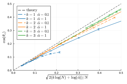
We see that cosθcsubscript𝜃𝑐\cos\theta_{c} goes to zero proportionally to logN/N𝑁𝑁\sqrt{\log N/N}. Therefore, using the dense associative memory network at a storage capacity that is much smaller than its (exponentially large ) threshold leads to a very large basin of attraction. We have tested this prediction in the case of spherical patterns. The results, presented in Fig. 5, are in very good agreement with the theory.
Refer to caption
Figure 5: Size of attraction basins for patterns uniformly distributed on the hypersphere. We study here the case in which the number of stored patterns is polynomial, P=α~Nk𝑃~𝛼superscript𝑁𝑘P=\tilde{\alpha}N^{k}, far below its exponential storage capacity. Given a pattern 𝝃1superscript𝝃1\operatorname{\bm{\xi}}^{1}, we compute the cosine of the average angle to the nearest other pattern. We plot the expectation value of this cosine versus the theoretical prediction 2klogN+logα~N2𝑘𝑁~𝛼𝑁\sqrt{2\frac{k\log N+\log\tilde{\alpha}}{N}}. In the large N𝑁N limit, there is good agreement between the numerical result and the prediction.

Appendix C Spherical patterns

C.1 Typical case

Consider the case where patterns 𝝃μNsuperscript𝝃𝜇superscript𝑁\operatorname{\bm{\xi}}^{\mu}\in\mathbb{R}^{N} are uniformly distributed on the sphere 𝝃μ2=Nsuperscriptdelimited-∥∥superscript𝝃𝜇2𝑁\lVert\operatorname{\bm{\xi}}^{\mu}\rVert^{2}=N, and choose a vector 𝐱𝐱\operatorname{\mathbf{x}} such that 𝐱2=ρ2Nsuperscriptdelimited-∥∥𝐱2superscript𝜌2𝑁\lVert\operatorname{\mathbf{x}}\rVert^{2}=\rho^{2}N. Using rotational invariance, the distribution of the energy levels εμ=𝐱𝝃μ/Nsuperscript𝜀𝜇𝐱superscript𝝃𝜇𝑁{\varepsilon}^{\mu}=\operatorname{\mathbf{x}}\cdot\operatorname{\bm{\xi}}^{\mu}/N depends on 𝐱𝐱\operatorname{\mathbf{x}} only through ρ𝜌\rho. One can choose the axes so that εμ=ρξ1μ/Nsuperscript𝜀𝜇𝜌subscriptsuperscript𝜉𝜇1𝑁{\varepsilon}^{\mu}=\rho\xi^{\mu}_{1}/\sqrt{N}. The probability density of these energy levels is expressed by the large deviation function

sρ(ε)=limN1Nlogidξiδ(Niξi2)δ(ερξ1N)idξiδ(Niξi2).subscript𝑠𝜌𝜀subscript𝑁1𝑁subscriptproduct𝑖𝑑subscript𝜉𝑖𝛿𝑁subscript𝑖superscriptsubscript𝜉𝑖2𝛿𝜀𝜌subscript𝜉1𝑁subscriptproduct𝑖𝑑subscript𝜉𝑖𝛿𝑁subscript𝑖superscriptsubscript𝜉𝑖2s_{\rho}({\varepsilon})=-\lim_{N\to\infty}\frac{1}{N}\log\frac{\int\prod_{i}d\xi_{i}\ \delta\left(N-\sum_{i}\xi_{i}^{2}\right)\,\delta\left({\varepsilon}-\frac{\rho\xi_{1}}{\sqrt{N}}\right)}{\int\prod_{i}d\xi_{i}\ \delta\left(N-\sum_{i}\xi_{i}^{2}\right)}. (49)

As prescribed in Appendix A.3, we first compute its Legendre transform

ζρ(λ)=limN1Nlogidξiδ(Niξi2)eλρξ1Nidξiδ(Niξi2).subscript𝜁𝜌𝜆subscript𝑁1𝑁subscriptproduct𝑖𝑑subscript𝜉𝑖𝛿𝑁subscript𝑖superscriptsubscript𝜉𝑖2superscript𝑒𝜆𝜌subscript𝜉1𝑁subscriptproduct𝑖𝑑subscript𝜉𝑖𝛿𝑁subscript𝑖superscriptsubscript𝜉𝑖2\zeta_{\rho}(\lambda)=\lim_{N\to\infty}\frac{1}{N}\log\frac{\int\prod_{i}d\xi_{i}\ \delta\left(N-\sum_{i}\xi_{i}^{2}\right)e^{\lambda\rho\xi_{1}\sqrt{N}}}{\int\prod_{i}d\xi_{i}\ \delta\left(N-\sum_{i}\xi_{i}^{2}\right)}. (50)

Standard field theoretical calculations and saddle point evaluation lead to

ζρ(λ)=12(1+4λ2ρ21log(1+1+4λ2ρ22)).subscript𝜁𝜌𝜆1214superscript𝜆2superscript𝜌21114superscript𝜆2superscript𝜌22\zeta_{\rho}(\lambda)=\frac{1}{2}\left(\sqrt{1+4\lambda^{2}\rho^{2}}-1-\log\left(\frac{1+\sqrt{1+4\lambda^{2}\rho^{2}}}{2}\right)\right)\ . (51)

Performing the inverse Legendre transform one gets

sρ(ε)subscript𝑠𝜌𝜀\displaystyle s_{\rho}({\varepsilon}) =12log(1ε2ρ2).absent121superscript𝜀2superscript𝜌2\displaystyle=-\frac{1}{2}\log\left(1-\frac{{\varepsilon}^{2}}{\rho^{2}}\right). (52)

The function sρ(ε)subscript𝑠𝜌𝜀s_{\rho}({\varepsilon}) is shown in Fig. 4. According to Eq. (28), the REM free-energy density is given by

ϕα,ρ(λ)={αλ+12λ(1+4λ2ρ21log(1+1+4λ2ρ22]))λ<λ(α,ρ)ρ1e2αλλ(α,ρ),\displaystyle\phi_{\alpha,\rho}(\lambda)=\begin{cases}\frac{\alpha}{\lambda}+\frac{1}{2\lambda}\left(\sqrt{1+4\lambda^{2}\rho^{2}}-1-\log\left(\frac{1+\sqrt{1+4\lambda^{2}\rho^{2}}}{2}\right])\right)&\lambda<\lambda_{*}(\alpha,\rho)\\ \rho\sqrt{1-e^{-2\alpha}}&\lambda\geq\lambda_{*}(\alpha,\rho),\end{cases}

where

λ(α,ρ)=1ρe2α1e2α.subscript𝜆𝛼𝜌1𝜌superscript𝑒2𝛼1superscript𝑒2𝛼\displaystyle\lambda_{*}(\alpha,\rho)=\frac{1}{\rho}e^{2\alpha}\sqrt{1-e^{-2\alpha}}. (53)

According to Eq. (7), the phase boundary for the retrieval of a typical pattern, α1(λ)subscript𝛼1𝜆\alpha_{1}(\lambda), is found by using the expression for ϕα,ρsubscriptitalic-ϕ𝛼𝜌\phi_{\alpha,\rho} with ρ=1𝜌1\rho=1 (which is the radius of any pattern). It is given by the value of α𝛼\alpha satisfying that ϕα,1(λ)=1subscriptitalic-ϕ𝛼1𝜆1\phi_{\alpha,1}(\lambda)=1. This is plotted in Fig. 1. The retrieval phase boundary is entirely in the region of the REM which is uncondensed.

C.2 All patterns retrieval

In order to study the retrieval of all patterns using the union bound, we notice that, for the spherical model, all patterns have r=𝝃1/N=1𝑟delimited-∥∥superscript𝝃1𝑁1r=\lVert\operatorname{\bm{\xi}}^{1}\rVert/\sqrt{N}=1. Therefore, eq. (9) reduces to

A(α,λ)=infϕ:ϕ>1Iα,1,λ(ϕ)𝐴𝛼𝜆subscriptinfimum:italic-ϕitalic-ϕ1subscript𝐼𝛼1𝜆italic-ϕ\displaystyle A(\alpha,\lambda)=\inf_{\phi\,:\phi>1}I_{\alpha,1,\lambda}(\phi) (54)

Assuming α<α1(λ)𝛼subscript𝛼1𝜆\alpha<\alpha_{1}(\lambda), by the very definition of α1subscript𝛼1\alpha_{1} we have that the typical REM free energy ϕα,1(λ)subscriptitalic-ϕ𝛼1𝜆\phi_{\alpha,1}(\lambda) is lower than 1. Therefore, we should look at atypically high free energy. According to Eq. (8) we have

A(α,λ)=infϕ:ϕ>1s1(ϕ)α.𝐴𝛼𝜆subscriptinfimum:italic-ϕitalic-ϕ1subscript𝑠1italic-ϕ𝛼A(\alpha,\lambda)=\inf_{\phi\,:\phi>1}s_{1}(\phi)-\alpha. (55)

On the other hand, Eq. (52) implies that s1(ϕ)subscript𝑠1italic-ϕs_{1}(\phi) is finite only for ϕ<1italic-ϕ1\phi<1. Therefore A(α,λ)=+𝐴𝛼𝜆A(\alpha,\lambda)=+\infty for α<α1(λ)𝛼subscript𝛼1𝜆\alpha<\alpha_{1}(\lambda) and A(α,λ)=0𝐴𝛼𝜆0A(\alpha,\lambda)=0 otherwise. This leads to the final result αclb(λ)=αc(λ)=α1(λ)superscriptsubscript𝛼clb𝜆subscript𝛼𝑐𝜆subscript𝛼1𝜆\operatorname{\alpha_{c}^{lb}}(\lambda)=\alpha_{c}(\lambda)=\alpha_{1}(\lambda) for spherical patterns.

C.3 Attraction basins

The attraction basins are studied by considering an initial condition 𝐱𝐱\operatorname{\mathbf{x}} on the sphere 𝐱2=Nsuperscriptdelimited-∥∥𝐱2𝑁\lVert\operatorname{\mathbf{x}}\rVert^{2}=N sampled uniformly at random but at fixed angle cos(θ)=𝐱𝝃1/N𝜃𝐱superscript𝝃1𝑁\cos(\theta)=\operatorname{\mathbf{x}}\cdot\operatorname{\bm{\xi}}^{1}/N from a typical pattern (𝝃1superscript𝝃1\operatorname{\bm{\xi}}^{1} without loss of generality). As argued in Sec. IV, the gradient flow (with or without projection on the sphere) will converge to 𝝃1superscript𝝃1\operatorname{\bm{\xi}}^{1} as long as the initial angle is smaller than some critical angle θc(α,λ)subscript𝜃𝑐𝛼𝜆\theta_{c}(\alpha,\lambda), that is cos(θ)>cos(θc)𝜃subscript𝜃𝑐\cos(\theta)>\cos(\theta_{c}). The critical angle is found solving ϕα,1(λ)=cos(θc)subscriptitalic-ϕ𝛼1𝜆subscript𝜃𝑐\phi_{\alpha,1}(\lambda)=\cos(\theta_{c}) as suggested by the energy decomposition (3). The critical lines are shown in Fig. 2. For a given α𝛼\alpha, the largest basin size is obtained for λe2α1e2α𝜆superscript𝑒2𝛼1superscript𝑒2𝛼\lambda\geq e^{2\alpha}\sqrt{1-e^{-2\alpha}}, where the critical angle becomes cosθc(α)=1e2αsubscript𝜃c𝛼1superscript𝑒2𝛼\operatorname{\cos\theta_{c}}(\alpha)=\sqrt{1-e^{-2\alpha}}.

Appendix D Gaussian patterns

D.1 Typical case

Consider the case where patterns have independent identically distributed components which are Gaussian variables of mean zero and unity variance, and independently choose a vector 𝐱𝐱\operatorname{\mathbf{x}} such that 𝐱2=Nρ2delimited-∥∥superscript𝐱2𝑁superscript𝜌2\lVert\operatorname{\mathbf{x}}^{2}\rVert=N\rho^{2}. Using rotational invariance, the distribution of the energy levels εμ=𝐱𝝃μ/Nsuperscript𝜀𝜇𝐱superscript𝝃𝜇𝑁{\varepsilon}^{\mu}=\operatorname{\mathbf{x}}\cdot\operatorname{\bm{\xi}}^{\mu}/N depends on 𝐱𝐱\operatorname{\mathbf{x}} only through its norm ρ𝜌\rho. One can choose the axes so that εμ=ρξ1μ/Nsuperscript𝜀𝜇𝜌subscriptsuperscript𝜉𝜇1𝑁{\varepsilon}^{\mu}=\rho\xi^{\mu}_{1}/\sqrt{N}. The probability density of this energy is expressed by the large deviation function

sρ(ε)=limN1Nlog(dξ12πeξ12/2δ(ερξ1N)).subscript𝑠𝜌𝜀subscript𝑁1𝑁𝑑subscript𝜉12𝜋superscript𝑒superscriptsubscript𝜉122𝛿𝜀𝜌subscript𝜉1𝑁s_{\rho}({\varepsilon})=-\lim_{N\to\infty}\frac{1}{N}\log\left(\int\frac{d\xi_{1}}{\sqrt{2\pi}}\;e^{-\xi_{1}^{2}/2}\;\delta\left({\varepsilon}-\frac{\rho\xi_{1}}{\sqrt{N}}\right)\right). (56)

The generating function is given instead by

ζρ(ε)=limN1Nlogdξ12πeξ12/2+1Nλρξ1,subscript𝜁𝜌𝜀subscript𝑁1𝑁𝑑subscript𝜉12𝜋superscript𝑒superscriptsubscript𝜉1221𝑁𝜆𝜌subscript𝜉1\zeta_{\rho}({\varepsilon})=\lim_{N\to\infty}\frac{1}{N}\log\int\frac{d\xi_{1}}{\sqrt{2\pi}}\;e^{-\xi_{1}^{2}/2+\frac{1}{\sqrt{N}}\lambda\rho\xi_{1}}, (57)

and the two functions are connected by a Legendre transform as described in Appendix A.1.

Computing the two limits obtain

sρ(ε)subscript𝑠𝜌𝜀\displaystyle s_{\rho}({\varepsilon}) =ε22ρ2absentsuperscript𝜀22superscript𝜌2\displaystyle=\frac{{\varepsilon}^{2}}{2\rho^{2}} (58)
ζρ(λ)subscript𝜁𝜌𝜆\displaystyle\zeta_{\rho}(\lambda) =λ2ρ22.absentsuperscript𝜆2superscript𝜌22\displaystyle=\frac{\lambda^{2}\rho^{2}}{2}. (59)

The REM free-energy density, ϕα,ρ(λ)subscriptitalic-ϕ𝛼𝜌𝜆\phi_{\alpha,\rho}(\lambda), according to Eq. (28) reads

ϕα,ρ(λ)={αλ+12λρ2λ<λ(α,ρ)ρ2αλλ(α,ρ),subscriptitalic-ϕ𝛼𝜌𝜆cases𝛼𝜆12𝜆superscript𝜌2𝜆subscript𝜆𝛼𝜌𝜌2𝛼𝜆subscript𝜆𝛼𝜌\displaystyle\phi_{\alpha,\rho}(\lambda)=\begin{cases}\frac{\alpha}{\lambda}+\frac{1}{2}\lambda\rho^{2}&\lambda<\lambda_{*}(\alpha,\rho)\\ \rho\sqrt{2\alpha}&\lambda\geq\lambda_{*}(\alpha,\rho),\end{cases} (60)

where the condensation threshold is given by

λ(α,ρ)=2αρ.subscript𝜆𝛼𝜌2𝛼𝜌\displaystyle\lambda_{*}(\alpha,\rho)=\frac{\sqrt{2\alpha}}{\rho}. (61)

The phase boundary for retrieval of a typical pattern, α1(λ)subscript𝛼1𝜆\alpha_{1}(\lambda), is found by using the expression for ϕα,ρsubscriptitalic-ϕ𝛼𝜌\phi_{\alpha,\rho} with ρ=1𝜌1\rho=1 (which is the radius of a typical pattern) and finding the value of α𝛼\alpha such that ϕα,1(λ)=1subscriptitalic-ϕ𝛼1𝜆1\phi_{\alpha,1}(\lambda)=1. It takes the simple form

α1(λ)={λ(112λ)0λ<112λ1.subscript𝛼1𝜆cases𝜆112𝜆0𝜆112𝜆1\alpha_{1}(\lambda)=\begin{cases}\lambda(1-\frac{1}{2}\lambda)&0\leq\lambda<1\\ \frac{1}{2}&\lambda\geq 1.\end{cases} (62)

The phase diagram is plotted in Fig. 3.

D.2 All patterns retrieval

We now compute the quantities involved in the all patterns retrieval lower bound αclb(λ)superscriptsubscript𝛼clb𝜆\operatorname{\alpha_{c}^{lb}}(\lambda) given in Eq. (10). We first compute the large deviation rate function I~(r)~𝐼𝑟\tilde{I}(r) for the scaled norm of a single pattern, r=𝝃/N𝑟delimited-∥∥𝝃𝑁r=\lVert\operatorname{\bm{\xi}}\rVert/\sqrt{N}. It is easy to show that

I~(r)=limN1NlogdN𝝃2πNe(1/2)iξi2δ(r𝝃N)=12(r21)logr.~𝐼𝑟subscript𝑁1𝑁superscript𝑑𝑁𝝃superscript2𝜋𝑁superscript𝑒12subscript𝑖superscriptsubscript𝜉𝑖2𝛿𝑟delimited-∥∥𝝃𝑁12superscript𝑟21𝑟\displaystyle\tilde{I}(r)=-\lim_{N\to\infty}\frac{1}{N}\;\log\int\frac{d^{N}\operatorname{\bm{\xi}}}{\sqrt{2\pi}^{N}}\;e^{-(1/2)\sum_{i}\xi_{i}^{2}}\;\delta\left(r-\frac{\lVert\operatorname{\bm{\xi}}\rVert}{\sqrt{N}}\right)=\frac{1}{2}(r^{2}-1)-\log r. (63)

Then we compute the large deviation function for the REM free energy conditioned on the pattern radius r𝑟r. According to the general expression in Eq. (8), this is given by

Iα,r,λ(ϕ)={+ϕ<ϕα,r(λ)0ϕ=ϕα,r(λ)ϕ22r2αϕ>ϕα,r(λ).subscript𝐼𝛼𝑟𝜆italic-ϕcasesitalic-ϕsubscriptitalic-ϕ𝛼𝑟𝜆0italic-ϕsubscriptitalic-ϕ𝛼𝑟𝜆superscriptitalic-ϕ22superscript𝑟2𝛼italic-ϕsubscriptitalic-ϕ𝛼𝑟𝜆I_{\alpha,r,\lambda}(\phi)=\begin{cases}+\infty&\phi<\phi_{\alpha,r}(\lambda)\\ 0&\phi=\phi_{\alpha,r}(\lambda)\\ \frac{\phi^{2}}{2r^{2}}-\alpha&\phi>\phi_{\alpha,r}(\lambda).\end{cases} (64)

For convenience , we define the function I(α,r,λ)superscript𝐼𝛼𝑟𝜆I^{*}(\alpha,r,\lambda) such that Eq. (9) becomes:

A(α,λ)=infr[0,)I~(r)+I(α,r,λ),𝐴𝛼𝜆subscriptinfimum𝑟0~𝐼𝑟subscript𝐼𝛼𝑟𝜆\displaystyle A(\alpha,\lambda)=\inf_{r\in[0,\infty)}\,\tilde{I}(r)+I_{*}(\alpha,r,\lambda), (65)

that is

I(α,r,λ)=infϕ:ϕ>r2Iα,r,λ(ϕ).subscript𝐼𝛼𝑟𝜆subscriptinfimum:italic-ϕitalic-ϕsuperscript𝑟2subscript𝐼𝛼𝑟𝜆italic-ϕI_{*}(\alpha,r,\lambda)=\inf_{\phi\,:\phi>r^{2}}I_{\alpha,r,\lambda}(\phi). (66)

Let us denote by r0(α,λ)subscript𝑟0𝛼𝜆r_{0}(\alpha,\lambda) the value of r𝑟r such that r2=ϕα,r(λ)superscript𝑟2subscriptitalic-ϕ𝛼𝑟𝜆r^{2}=\phi_{\alpha,r}(\lambda). It is given by

r0(α,λ)={αλ(1λ/2)0λ<12αλ1.subscript𝑟0𝛼𝜆cases𝛼𝜆1𝜆20𝜆12𝛼𝜆1r_{0}(\alpha,\lambda)=\begin{cases}\sqrt{\frac{\alpha}{\lambda(1-\lambda/2)}}&0\leq\lambda<1\\ \sqrt{2\alpha}&\lambda\geq 1.\end{cases} (67)

When r<r0𝑟subscript𝑟0r<r_{0}, we have ϕα,r(λ)>r2subscriptitalic-ϕ𝛼𝑟𝜆superscript𝑟2\phi_{\alpha,r}(\lambda)>r^{2}. When r>r0𝑟subscript𝑟0r>r_{0} instead, we have ϕα,r(λ)<r2subscriptitalic-ϕ𝛼𝑟𝜆superscript𝑟2\phi_{\alpha,r}(\lambda)<r^{2}. It follows that:

  • If r>r0𝑟subscript𝑟0r>r_{0} the infimum in (66) is obtained at ϕ=r2italic-ϕsuperscript𝑟2\phi=r^{2} and its value is I(α,r,λ)=r22αsubscript𝐼𝛼𝑟𝜆superscript𝑟22𝛼I_{*}(\alpha,r,\lambda)=\frac{r^{2}}{2}-\alpha.

  • If r<r0𝑟subscript𝑟0r<r_{0} the infimum in (66) is obtained at ϕ=ϕα,r(λ)italic-ϕsubscriptitalic-ϕ𝛼𝑟𝜆\phi=\phi_{\alpha,r}(\lambda) and its value is I(α,r,λ)=0subscript𝐼𝛼𝑟𝜆0I_{*}(\alpha,r,\lambda)=0.

This leads to

A(α,λ)=min(minr[0,r0(α,λ)]I~(r),minr[r0(α,λ),)I~(r)+r22α).𝐴𝛼𝜆subscript𝑟0subscript𝑟0𝛼𝜆~𝐼𝑟subscript𝑟subscript𝑟0𝛼𝜆~𝐼𝑟superscript𝑟22𝛼A(\alpha,\lambda)=\min\left(\min_{r\in[0,r_{0}(\alpha,\lambda)]}\,\tilde{I}(r),\ \min_{r\in[r_{0}(\alpha,\lambda),\infty)}\,\tilde{I}(r)+\frac{r^{2}}{2}-\alpha\right). (68)

The final value for αclb(λ)superscriptsubscript𝛼clb𝜆\operatorname{\alpha_{c}^{lb}}(\lambda) is found by solving A(α,λ)=α𝐴𝛼𝜆𝛼A(\alpha,\lambda)=\alpha. When λ0.70091greater-than-or-equivalent-to𝜆0.70091\lambda\gtrsim 0.70091 one gets αclb=log(2)/4superscriptsubscript𝛼clb24\operatorname{\alpha_{c}^{lb}}=\log(2)/4. We have αclbλsimilar-tosuperscriptsubscript𝛼clb𝜆\operatorname{\alpha_{c}^{lb}}\sim\lambda instead for small λ𝜆\lambda, therefore in this limit it matches α1(λ)subscript𝛼1𝜆\alpha_{1}(\lambda). The results are shown in Fig. 3.

D.3 Attraction basins and typical distances

In the case of Gaussian patterns, the condition ρrξcos(θ)>ϕα,ρ(λ)𝜌subscript𝑟𝜉𝜃subscriptitalic-ϕ𝛼𝜌𝜆\rho\,r_{\xi}\,\cos(\theta)>\phi_{\alpha,\rho}(\lambda) identifying the attraction basin of a typical pattern, for large λ𝜆\lambda takes the form cos(θc)>2αsubscript𝜃𝑐2𝛼\cos(\theta_{c})>\sqrt{2\alpha}. Clearly, the basin disappears when α>0.5𝛼0.5\alpha>0.5

Since in this ensemble we have large deviations also in the patterns’ radii, contrary to the spherical case, we can perform a slightly more refined version of the computation in Appendix B in order to compute also the radius of the patterns with maximum overlap with a reference configuration.

Consider a reference configuration 𝐱𝐱\operatorname{\mathbf{x}} with squared norm 𝐱2=Nsuperscriptdelimited-∥∥𝐱2𝑁\lVert\operatorname{\mathbf{x}}\rVert^{2}=N. We ask what is the number of patterns with a certain overlap c𝑐c with it and with a certain square norm r2Nsuperscript𝑟2𝑁r^{2}N. That is, we want to compute the statistics of the random variable

𝖭(c,r)=μ=2Pδ(𝐱𝝃μcN)δ(𝝃μ2r2N)𝖭𝑐𝑟superscriptsubscript𝜇2𝑃𝛿𝐱superscript𝝃𝜇𝑐𝑁𝛿superscriptdelimited-∥∥superscript𝝃𝜇2superscript𝑟2𝑁\mathsf{N}(c,r)=\sum_{\mu=2}^{P}\delta\left(\operatorname{\mathbf{x}}\cdot\operatorname{\bm{\xi}}^{\mu}-cN\right)\,\delta\left(\lVert\operatorname{\bm{\xi}}^{\mu}\rVert^{2}-r^{2}N\right) (69)

Although we are interested in the quenched average, 1N𝔼log𝖭(c,r)1𝑁𝔼𝖭𝑐𝑟\frac{1}{N}\mathbb{E}\log\mathsf{N}(c,r), let’s do an annealed computation first.

𝔼𝖭(c,r)𝔼𝖭𝑐𝑟\displaystyle\mathbb{E}\mathsf{N}(c,r) =eαN𝔼dc^2πdr^2πe+ic^cN+12r^r2Niq^ixiξi12r^i(ξi)2absentsuperscript𝑒𝛼𝑁𝔼𝑑^𝑐2𝜋𝑑^𝑟2𝜋superscript𝑒𝑖^𝑐𝑐𝑁12^𝑟superscript𝑟2𝑁𝑖^𝑞subscript𝑖subscript𝑥𝑖subscript𝜉𝑖12^𝑟subscript𝑖superscriptsubscript𝜉𝑖2\displaystyle=e^{\alpha N}\mathbb{E}\int\frac{d\hat{c}}{2\pi}\,\frac{d\hat{r}}{2\pi}\ e^{+i\hat{c}cN+\frac{1}{2}\hat{r}r^{2}N-i\hat{q}\sum_{i}x_{i}\xi_{i}-\frac{1}{2}\hat{r}\sum_{i}\left(\xi_{i}\right)^{2}} (70)
=dc^2π/Ndr^2π/NeαN+ic^cN+12r^r2Nc^22(1+r^)N12Nlog(1+r^)absent𝑑^𝑐2𝜋𝑁𝑑^𝑟2𝜋𝑁superscript𝑒𝛼𝑁𝑖^𝑐𝑐𝑁12^𝑟superscript𝑟2𝑁superscript^𝑐221^𝑟𝑁12𝑁1^𝑟\displaystyle=\int\frac{d\hat{c}}{2\pi/N}\,\frac{d\hat{r}}{2\pi/N}\ e^{\alpha N+i\hat{c}cN+\frac{1}{2}\hat{r}r^{2}N-\frac{\hat{c}^{2}}{2(1+\hat{r})}N-\frac{1}{2}N\log(1+\hat{r})} (71)
=dr^2π(1+r^)/NeαN+12r^r212c2(1+r^)N12Nlog(1+r^)absent𝑑^𝑟2𝜋1^𝑟𝑁superscript𝑒𝛼𝑁12^𝑟superscript𝑟212superscript𝑐21^𝑟𝑁12𝑁1^𝑟\displaystyle=\int\frac{d\hat{r}}{\sqrt{2\pi(1+\hat{r})/N}}\ e^{\alpha N+\frac{1}{2}\hat{r}r^{2}-\frac{1}{2}c^{2}(1+\hat{r})N-\frac{1}{2}N\log(1+\hat{r})} (72)

Therefore

limN+1Nlog𝔼𝖭(c,r)=α+12str^[r^r2c2(1+r^)log(1+r^)].subscript𝑁1𝑁𝔼𝖭𝑐𝑟𝛼12subscriptst^𝑟^𝑟superscript𝑟2superscript𝑐21^𝑟1^𝑟\lim_{N\to+\infty}\frac{1}{N}\log\mathbb{E}\mathsf{N}(c,r)=\alpha+\frac{1}{2}\operatorname{st}_{\hat{r}}\ \left[\hat{r}r^{2}-c^{2}(1+\hat{r})-\log(1+\hat{r})\right]. (73)

At the stationary point

r^=1r2c21.^𝑟1superscript𝑟2superscript𝑐21\hat{r}=\frac{1}{r^{2}-c^{2}}-1. (74)

This leads to

Sαann(c,r)=limN+1Nlog𝔼𝖭(c,r)=α+1r22+12log(r2c2)subscriptsuperscriptS𝑎𝑛𝑛𝛼𝑐𝑟subscript𝑁1𝑁𝔼𝖭𝑐𝑟𝛼1superscript𝑟2212superscript𝑟2superscript𝑐2\mathrm{S}^{ann}_{\alpha}(c,r)=\lim_{N\to+\infty}\frac{1}{N}\log\mathbb{E}\mathsf{N}(c,r)=\alpha+\frac{1-r^{2}}{2}+\frac{1}{2}\log\left(r^{2}-c^{2}\right) (75)

A standard second moment argument then gives the concentration of the quenched entropy:

Sα(c,r)=limN1NlogN(c)={Sαann(c,r)Sαann(c,r)0Sαann(c,r)<0subscript𝑆𝛼𝑐𝑟subscript𝑁1𝑁N𝑐casessubscriptsuperscriptS𝑎𝑛𝑛𝛼𝑐𝑟subscriptsuperscriptS𝑎𝑛𝑛𝛼𝑐𝑟0subscriptsuperscriptS𝑎𝑛𝑛𝛼𝑐𝑟0S_{\alpha}(c,r)=\lim_{N\to\infty}\frac{1}{N}\log\mathrm{N}(c)=\begin{cases}\mathrm{S}^{ann}_{\alpha}(c,r)&\mathrm{S}^{ann}_{\alpha}(c,r)\geq 0\\ -\infty&\mathrm{S}^{ann}_{\alpha}(c,r)<0\end{cases} (76)

For a given overlap c𝑐c, the radius of the patterns giving the dominant contribution to the energy is found by setting rSαann(c,r)=0subscript𝑟subscriptsuperscriptS𝑎𝑛𝑛𝛼𝑐𝑟0\partial_{r}\mathrm{S}^{ann}_{\alpha}(c,r)=0. This gives

r(c)subscript𝑟𝑐\displaystyle r_{*}(c) =1+c2,absent1superscript𝑐2\displaystyle=\sqrt{1+c^{2}}, (77)
Sαann(c)subscriptsuperscriptS𝑎𝑛𝑛𝛼𝑐\displaystyle\mathrm{S}^{ann}_{\alpha}(c) =Sαann(c,r(c))=α12c2absentsubscriptsuperscriptS𝑎𝑛𝑛𝛼𝑐subscript𝑟𝑐𝛼12superscript𝑐2\displaystyle=\mathrm{S}^{ann}_{\alpha}(c,r_{*}(c))=\alpha-\frac{1}{2}c^{2} (78)

Imposing the condition Sαann(c,r(c))=0subscriptsuperscriptS𝑎𝑛𝑛𝛼𝑐subscript𝑟𝑐0\mathrm{S}^{ann}_{\alpha}(c,r_{*}(c))=0 we finally recover the result cmax(α)=2αsubscript𝑐𝑚𝑎𝑥𝛼2𝛼c_{max}(\alpha)=\sqrt{2\alpha}.

Appendix E Storage capacity lower bound from Ramsauer et al. ’20

In this Appendix, we restate Theorem 3 of Ref. [8] using our notation and we compute its asymptotic form in the high-dimensional limit N+𝑁N\to+\infty with P=eαN𝑃superscript𝑒𝛼𝑁P=e^{\alpha N} for fixed α𝛼\alpha. The Theorem considers patterns 𝝃μsuperscript𝝃𝜇\operatorname{\bm{\xi}}^{\mu} uniformly distributed on the sphere of radius KN1𝐾𝑁1K\sqrt{N-1} and provides a lower bound for all patterns retrieval capacity at finite N𝑁N described in the following. We consider K=1𝐾1K=1 for simplicity and assume failure probability 0<p10𝑝10<p\leq 1 for the storage problem, that is the probability that at least one pattern is not an approximate fixed point of the dynamics (we refer the reader to Ref. [8] for precise definitions). We define the quantities

a:=2N1(1+log(2λp(N1)));b:=25λ;c:=bW0(ea+logb);formulae-sequenceassign𝑎2𝑁112𝜆𝑝𝑁1formulae-sequenceassign𝑏25𝜆assign𝑐𝑏subscript𝑊0superscript𝑒𝑎𝑏\displaystyle a:=\frac{2}{N-1}\left(1+\log(2\lambda p(N-1))\right);\quad b:=\frac{2}{5}\lambda;\quad c:=\frac{b}{W_{0}(e^{a+\log b})}; (79)

where W0subscript𝑊0W_{0} is the upper branch of the Lambert W𝑊W function. Ensuring c(2p)N14𝑐superscript2𝑝𝑁14c\geq\left(\frac{2}{\sqrt{p}}\right)^{\frac{N-1}{4}}, with probability 1p1𝑝1-p the number of patterns that can be stored Pcsubscript𝑃𝑐P_{c} satisfies the bound [8]

Pc>pcN14.subscript𝑃𝑐𝑝superscript𝑐𝑁14P_{c}>\sqrt{p}c^{\frac{N-1}{4}}. (80)

We now consider the thermodynamic limit N,P𝑁𝑃N,P\to\infty and p0𝑝0p\to 0 with:

p𝑝\displaystyle p =eγN,absentsuperscript𝑒𝛾𝑁\displaystyle=e^{-\gamma N}, (81)
Pcsubscript𝑃𝑐\displaystyle P_{c} =eαcN.absentsuperscript𝑒subscript𝛼𝑐𝑁\displaystyle=e^{\alpha_{c}N}. (82)

The limit for the previously defined quantitis is then

a=2γ;b=25;λc=25λ1W0(e2γ+log(25λ)).formulae-sequence𝑎2𝛾formulae-sequence𝑏25𝜆𝑐25𝜆1subscript𝑊0superscript𝑒2𝛾25𝜆\displaystyle a=-2\gamma;\quad b=\frac{2}{5};\lambda\quad c=\frac{2}{5}\lambda\frac{1}{W_{0}\left(e^{-2\gamma+\log\left(\frac{2}{5}\lambda\right)}\right)}. (83)

The inequality (80) becomes

αc>12γ+14logc.subscript𝛼𝑐12𝛾14𝑐\alpha_{c}>-\frac{1}{2}\gamma+\frac{1}{4}\log c. (84)

Taking the limit γ0𝛾0\gamma\to 0 we finally derived the asymptotic form of the bound presented in Ref. [8]:

αc(λ)>14log[2λ/5W0(2λ/5)]αc,ramslb(λ)subscript𝛼𝑐𝜆142𝜆5subscript𝑊02𝜆5superscriptsubscript𝛼cramslb𝜆\alpha_{c}(\lambda)>\frac{1}{4}\log\left[\frac{2\lambda/5}{W_{0}(2\lambda/5)}\right]\eqqcolon\operatorname{\alpha_{c,\text{rams}}^{lb}}(\lambda) (85)

For large λ𝜆\lambda we have c2λ5log(25λ)similar-to𝑐2𝜆525𝜆c\sim\frac{2\lambda}{5\log(\frac{2}{5}\lambda)} and αc,ramslb14logλsimilar-tosuperscriptsubscript𝛼cramslb14𝜆\operatorname{\alpha_{c,\text{rams}}^{lb}}\sim\frac{1}{4}\log\lambda. For small λ𝜆\lambda instead we have αc,ramslbλ/10similar-tosuperscriptsubscript𝛼cramslb𝜆10\operatorname{\alpha_{c,\text{rams}}^{lb}}\sim\lambda/10. The value of αc,ramslbsuperscriptsubscript𝛼cramslb\operatorname{\alpha_{c,\text{rams}}^{lb}} is plotted in Fig. 1. One can notice a large gap with the exact value obtained by our large deviation analysis.

Appendix F Numerical Experiments

This Appendix is devoted to the numerical validation of our analytical result for the typical pattern retrieval threshold α1(λ)subscript𝛼1𝜆\alpha_{1}(\lambda) (more precisely, we consider its inverse, λ1(α)subscript𝜆1𝛼\lambda_{1}(\alpha)) and for the typical basin size. We make the general remark that while the numerical results are in good agreement with theory predictions for infinite N𝑁N, dealing with an exponential number of patterns makes the system hard to simulate. We quickly saturate our memory and compute resources going up in N𝑁N so that is hard to extrapolate the large N𝑁N behavior. Therefore, the numerical validation of our theory cannot be made entirely satisfactory, and we hope that follow-up works will be able to establish with mathematical rigor our results obtained through partially non-rigorous arguments.

In the numerical experiments, we perform a gradient descent (GD) procedure on the energy function of Eq. (1). We use a step size η=0.5𝜂0.5\eta=0.5. The results are averaged over a number of realizations of the patterns that vary from 100010001000 (low values of N𝑁N and α𝛼\alpha) to 10 (large N𝑁N and α𝛼\alpha).

F.1 Typical pattern retrieval

In the first set of experiments, we start from the initial condition 𝐱t=0=𝝃1superscript𝐱𝑡0superscript𝝃1\operatorname{\mathbf{x}}^{t=0}=\operatorname{\bm{\xi}}^{1} and run GD until convergence. We then plot the normalized distance from the initial configuration, Δ=𝐱t=𝝃12/NΔsuperscriptdelimited-∥∥superscript𝐱𝑡superscript𝝃12𝑁\Delta=\lVert\operatorname{\mathbf{x}}^{t=\infty}-\operatorname{\bm{\xi}}^{1}\rVert^{2}/N, as a function of λ𝜆\lambda and for different values of N𝑁N and α𝛼\alpha. The results are presented in Fig. 6 for the spherical case and in Fig. 7 for the Gaussian case. In both cases, at large λ𝜆\lambda GD remains close to the initial point, meaning that the pattern is an (approximate) minimum. For low λ𝜆\lambda GD approaches the origin instead, a phenomenon already outlined in Ref. [8] as the ”average of all patterns” global fixed point. As expected, the crossover between the two regimes becomes sharper as N𝑁N increases and approaches the analytical prediction for the threshold λ1(α)subscript𝜆1𝛼\lambda_{1}(\alpha) obtained by inverting Eq. (7). We notice that the transition is much smoother in the Gaussian case compared to the spherical case.

In Fig. 1 (bottom), we present a large N𝑁N extrapolation in the case of spherical patterns. At given α𝛼\alpha and N𝑁N, we define the crossover value of λ𝜆\lambda as the smallest value of λ𝜆\lambda for which Δ<0.5Δ0.5\Delta<0.5. We then extrapolate the numerical results to large N𝑁N through a quadratic fit in 1N1𝑁\frac{1}{N} and compare them with the analytical prediction λ1(α)subscript𝜆1𝛼\lambda_{1}(\alpha).

Refer to caption
Figure 6: Spherical patterns. End distance ΔΔ\Delta from initial conditions 𝝃1superscript𝝃1\operatorname{\bm{\xi}}^{1} under GD dynamics as a function of the interaction strength λ𝜆\lambda and for different values of N𝑁N and α𝛼\alpha. Vertical lines are the predicted values for the threshold λ1(α)subscript𝜆1𝛼\lambda_{1}(\alpha) at infinite N𝑁N separating the retrieval and the non-retrieval regime.
Refer to caption
Figure 7: Gaussian patterns. End distance ΔΔ\Delta from initial conditions 𝝃1superscript𝝃1\operatorname{\bm{\xi}}^{1} under GD dynamics as a function of the interaction strength λ𝜆\lambda and for different values of N𝑁N and α𝛼\alpha. Vertical lines are the predicted values for the threshold λ1(α)subscript𝜆1𝛼\lambda_{1}(\alpha) at infinite N𝑁N separating the retrieval and the non-retrieval regime.

F.2 All patterns retrieval for large λ𝜆\lambda

In the case of Gaussian patterns, we have a gap between the all patterns retrieval lower bound αclb(λ)superscriptsubscript𝛼clb𝜆\operatorname{\alpha_{c}^{lb}}(\lambda) of Eq. (10) and the single pattern one α1(λ)subscript𝛼1𝜆\alpha_{1}(\lambda), that is αclb(λ)<α1(λ)superscriptsubscript𝛼clb𝜆subscript𝛼1𝜆\operatorname{\alpha_{c}^{lb}}(\lambda)<\alpha_{1}(\lambda). This can be clearly seen in the phase diagram shown in Fig. 3. It remains to be established where the true value of the all patterns retrieval threshold αc(λ)subscript𝛼𝑐𝜆\alpha_{c}(\lambda) lies in the interval [αclb(λ),α1(λ)]superscriptsubscript𝛼clb𝜆subscript𝛼1𝜆[\operatorname{\alpha_{c}^{lb}}(\lambda),\alpha_{1}(\lambda)] and if the gap really exists. Since this question cannot be answered within the theory we have developed, we provide some indications through numerical simulations.

Due to computational constraints at large N𝑁N, we only explore the case of large λ𝜆\lambda here and drop the explicit λ𝜆\lambda dependence from the thresholds α1,αclb,αcsubscript𝛼1superscriptsubscript𝛼clbsubscript𝛼𝑐\alpha_{1},\operatorname{\alpha_{c}^{lb}},\alpha_{c}. For a given value of α𝛼\alpha and for a given realization of the patterns, we check if all patterns in the sample are stable (i.e. correspond to a local minimum of the energy). As α𝛼\alpha grows, the probability pNallretr(α)subscriptsuperscript𝑝allretr𝑁𝛼p^{\text{allretr}}_{N}(\alpha) of this event will drop to zero in correspondence of αcsubscript𝛼𝑐\alpha_{c}. The probability of the event ”all patterns are retrieved”, in the large λ𝜆\lambda case is defined by

pNallretr(α)=𝔼𝕀(𝝃μ2>𝝃μ𝝃νμ,ν[P]).subscriptsuperscript𝑝allretr𝑁𝛼𝔼𝕀formulae-sequencesuperscriptdelimited-∥∥superscript𝝃𝜇2superscript𝝃𝜇superscript𝝃𝜈for-all𝜇𝜈delimited-[]𝑃p^{\text{allretr}}_{N}(\alpha)=\mathbb{E}\ \mathbb{I}\left(\lVert\operatorname{\bm{\xi}}^{\mu}\rVert^{2}>\operatorname{\bm{\xi}}^{\mu}\cdot\operatorname{\bm{\xi}}^{\nu}\ \forall\mu,\nu\in[P]\right). (86)

This is to be compared with the probability of retrieving a typical pattern, that is the probability that most patterns are retrieved. This can be estimated by computing the expected fraction of retrieved patterns

fNretr(α)=𝔼1Pμ=1P𝕀(𝝃μ2>𝝃μ𝝃νν[P],νμ).f^{\text{retr}}_{N}(\alpha)=\mathbb{E}\frac{1}{P}\sum_{\mu=1}^{P}\mathbb{I}\left(\lVert\operatorname{\bm{\xi}}^{\mu}\rVert^{2}>\operatorname{\bm{\xi}}^{\mu}\cdot\operatorname{\bm{\xi}}^{\nu}\ \forall\nu\in[P],\nu\neq\mu\right). (87)

For large N𝑁N, the fraction fNretr(α)subscriptsuperscript𝑓retr𝑁𝛼f^{\text{retr}}_{N}(\alpha) should go from 1 to 0 at α1subscript𝛼1\alpha_{1}.

We estimate pNallretr(α)subscriptsuperscript𝑝allretr𝑁𝛼p^{\text{allretr}}_{N}(\alpha) and fNretr(α)subscriptsuperscript𝑓retr𝑁𝛼f^{\text{retr}}_{N}(\alpha) for different values of N𝑁N and α𝛼\alpha using Monte Carlo samples. The results are shown in Fig. 8. The estimated value of αcsubscript𝛼𝑐\alpha_{c}, where we observe the crossover from 1 to 0 for pNallretr(α)subscriptsuperscript𝑝allretr𝑁𝛼p^{\text{allretr}}_{N}(\alpha), seems to be close to the theoretically predicted αclb=log(2)/4superscriptsubscript𝛼clb24\operatorname{\alpha_{c}^{lb}}=\log(2)/4 and far from α1=0.5subscript𝛼10.5\alpha_{1}=0.5. It remains an open question whether we have αclb=αcsuperscriptsubscript𝛼clbsubscript𝛼𝑐\operatorname{\alpha_{c}^{lb}}=\alpha_{c} or not.

Refer to caption
Figure 8: Gaussian patterns ensemble. (Dashed Lines) Numerical estimations of the probability of retrieving all patterns P=eαN𝑃superscript𝑒𝛼𝑁P=e^{\alpha N} as a function of the load α𝛼\alpha, for large λ𝜆\lambda and for different system sizes N𝑁N. Vertical dashed line is the lower bound of Eq. (10) . (Continuous Lines) Fraction of patterns retrieved, also shown in the inset, converging to 1 at large N𝑁N in the range explored as expected since α<α1𝛼subscript𝛼1\alpha<\alpha_{1} .

F.3 Basins

In order to confirm our prediction cosθc=ϕα,1(λ)subscript𝜃𝑐subscriptitalic-ϕ𝛼1𝜆\cos\theta_{c}=\phi_{\alpha,1}(\lambda) for the basin size in the case of spherical patterns, we run the following experiments.

We sample an initial configuration for the GD dynamics uniformly at random on the hypersphere of radius N𝑁\sqrt{N} conditional on it being at a given angle θ𝜃\theta from 𝝃𝝃\operatorname{\bm{\xi}}. We then measure the normalized distance of the final configuration from 𝝃1superscript𝝃1\operatorname{\bm{\xi}}^{1} after convergence of GD. The result is shown in Fig. 9 (Left) for α=0.1,λ=0.2formulae-sequence𝛼0.1𝜆0.2\alpha=0.1,\lambda=0.2 and different values of N𝑁N as function of cos(θ)𝜃\cos(\theta). For small angle (cos(θ)𝜃\cos(\theta) close to 1), the final distance is close to 0, therefore the initial configuration lies in the basin of attraction of 𝝃1superscript𝝃1\operatorname{\bm{\xi}}^{1}. Increasing the angle we have a crossover to a regime where the configuration escapes from 𝝃1superscript𝝃1\operatorname{\bm{\xi}}^{1}. As N𝑁N increases the crossover becomes sharper and approaches the analytical prediction.

In Fig. 9 (Right) we plot the critical angle at finite size N𝑁N as a function of interaction strength. Since for finite N𝑁N we don’t have sharp thresholds, we define the critical angle as follows: for a given sample, the critical angle is defined as the one for which half of the random initializations of the dynamics (we use 10 restarts) fall back to 𝝃1superscript𝝃1\operatorname{\bm{\xi}}^{1} while the other half escape the basin. We apply a bisection method to find such angle and then average the (cosine of the) angle over 10 samples. As the plot shows, increasing the system size the curves converge to the infinite size theoretical prediction.
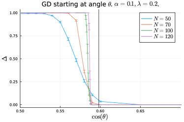
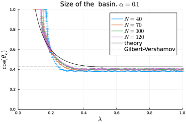
Refer to caption
Refer to caption
Figure 9: Spherical patterns. (Left) Distance ΔΔ\Delta from the reference pattern 𝝃1superscript𝝃1\operatorname{\bm{\xi}}^{1} as a function of the starting angle at the end of GD dynamics. We set α=0.1𝛼0.1\alpha=0.1 and λ=0.2𝜆0.2\lambda=0.2, with spherical patterns, and simulate different system sizes N𝑁N. The theory prediction for the critical angle is given by the vertical line. (Right) Critical angle for the basin as a function of interaction strength. Numerical simulations at finite size are compared to the theory prediction for infinite size and to the Gilbert-Varshamov result for the angle of the nearest pattern.

F.4 Scaled dot-product

In Fig. 10 we present numerical validation for single pattern retrieval threshold λ~1(α~)subscript~𝜆1~𝛼\tilde{\lambda}_{1}(\tilde{\alpha}) for the scaling regime discussed in Section VI in the case of Gaussian patterns. Here the number of patterns is P=exp(α~N1a)𝑃~𝛼superscript𝑁1𝑎P=\exp(\tilde{\alpha}N^{1-a}) and the energy reads

E(𝐱)=Naλ~logμeλ~Na𝐱𝝃μ+12𝐱2.𝐸𝐱superscript𝑁𝑎~𝜆subscript𝜇superscript𝑒~𝜆superscript𝑁𝑎𝐱superscript𝝃𝜇12superscriptdelimited-∥∥𝐱2E(\operatorname{\mathbf{x}})=-\frac{N^{a}}{\tilde{\lambda}}\log\sum_{\mu}e^{\frac{\tilde{\lambda}}{N^{a}}\operatorname{\mathbf{x}}\cdot\operatorname{\bm{\xi}}^{\mu}}+\frac{1}{2}\lVert\operatorname{\mathbf{x}}\rVert^{2}. (88)

The numerical protocol is the Gradient Descent one discussed in F.1. We observe that by increasing N𝑁N the retrieval crossover approaches the theoretical prediction as expected.

Refer to caption
Refer to caption
Figure 10: Gaussian patterns. Final distance from pattern 𝝃1superscript𝝃1\operatorname{\bm{\xi}}^{1} after GD for scaled attention with exponents a=1/2𝑎12a=1/2 (top) and a=3/4𝑎34a=3/4 (bottom). Vertical lines are the theoretical predictions λ1(α~)=α~subscript𝜆1~𝛼~𝛼\lambda_{1}(\tilde{\alpha})=\tilde{\alpha} for the retrieval transition. The patterns are sampled from the Gaussian ensemble.