HQP: A Human-Annotated Dataset for Detecting Online Propaganda

Abstract

Online propaganda poses a severe threat to the integrity of societies. However, existing datasets for detecting online propaganda have a key limitation: they were annotated using weak labels that can be noisy and even incorrect. To address this limitation, our work makes the following contributions: (1) We present HQP: a novel dataset ($N=$30,000$$) for detecting online propaganda with high-quality labels. To the best of our knowledge, HQP is the first dataset for detecting online propaganda that was created through human annotation. (2) We show empirically that state-of-the-art language models fail in detecting online propaganda when trained with weak labels (AUC: 64.03). In contrast, state-of-the-art language models can accurately detect online propaganda when trained with our high-quality labels (AUC: 92.25), which is an improvement of $\sim$44%. (3) To address the cost of labeling, we extend our work to few-shot learning. Specifically, we show that prompt-based learning using a small sample of high-quality labels can still achieve a reasonable performance (AUC: 80.27). Finally, we discuss implications for the NLP community to balance the cost and quality of labeling. Crucially, our work highlights the importance of high-quality labels for sensitive NLP tasks such as propaganda detection.

Disclaimer: Our work contains potentially offensive language and manipulative content. Reader’s discretion is advised.

1 Introduction

Propaganda refers to communication that is primarily used to influence, persuade, or manipulate public opinions Smith (2022). Nowadays, propaganda is widely used as practices of modern warfare (e.g., in the ongoing Russo-Ukrainian war) and thus poses a significant threat to the integrity of societies Kowalski (2022). In this regard, social media presents especially fertile grounds for disseminating propaganda at an unprecedented scale.

Existing NLP works for propaganda detection generally focus on different types of content. One literature stream aims at detecting propaganda in official news (e.g., Rashkin et al., 2017; Barrón-Cedeño et al., 2019; Da San Martino et al., 2019) but fails to detect propaganda in online content Wang et al. (2020). Another literature stream aims at detecting propaganda in online content from social media (Wang et al., 2020; Vijayaraghavan and Vosoughi, 2022). Here, existing works rely upon datasets that were exclusively annotated using weak labels and were, therefore, not validated by humans. Because of this, labels can be noisy and even incorrect. We later provide empirical support for this claim and show that the overlap between weak labels and human annotations is only $\sim$41%. Given that social media is increasingly used for propaganda dissemination Geissler et al. (2022), a tailored dataset is needed to tackle it. To the best of our knowledge, there is no dataset for detecting online propaganda that was constructed through human annotation and validation and thus comprises high-quality labels.

To fill this gap, we develop HQP: a novel dataset with high-quality labels for detecting online propaganda. HQP consists of $N=$30,000$$ tweets in English from the Russo-Ukrainian war. We use human annotation and validation to generate high-quality labels. Specifically, we follow best practices and make use of a rigorous multi-annotator, multi-batch procedure for annotation Song et al. (2020). We then leverage state-of-the-art, pre-trained language models (PLMs), i.e., BERT, RoBERTa, and BERTweet, to benchmark the performance in detecting online propaganda using weak labels vs. our high-quality labels. We find that high-quality labels are crucial for performance. We further acknowledge that human annotation also incurs labeling costs, and, to address this, we extend our work to few-shot learning (i.e., prompt-based learning).

Our main contributions are as follows:

1. We construct HQP, a novel dataset with high-quality labels for online propaganda detection using human-annotated labels.

2. We show that PLMs for detecting online propaganda using high-quality labels outperform PLMs using weak labels by a large margin.

3. We adapt few-short learning for online propaganda detection by prompting PLMs.

2 Related Work

Detecting harmful content: Prior literature in NLP has aimed to detect a broad spectrum of harmful content such as hate speech (e.g., Badjatiya et al., 2017; Mathew et al., 2021; Pavlopoulos et al., 2022), rumors (e.g., Zhou et al., 2019; Bian et al., 2020; Xia et al., 2020; Wei et al., 2021), and fake news (e.g., Zellers et al., 2019; Liu et al., 2020; Lu and Li, 2020; Jin et al., 2022). Further, claim detection has been studied, for example, in the context of the Russo-Ukrainian war La Gatta et al. (2023). Overall, literature for detecting harmful content makes widespread use of datasets that were created through human annotations (e.g., Founta et al., 2018; Thorne et al., 2018; Mathew et al., 2021), yet outside of online propaganda. We add by constructing a dataset through human annotations that is tailored to online propaganda.

Detecting propaganda content: Previous works for propaganda detection can be loosely grouped by the underlying content, namely (1) official news and (2) social media. We briefly review both in the following.

(1) News. To detect propaganda in official news, existing works leverage datasets that originate from propagandistic and non-propagandistic news outlets (Rashkin et al., 2017; Barrón-Cedeño et al., 2019; Da San Martino et al., 2019; Solopova et al., 2023), yet these datasets are not tailored to online content from social media. As a case in point, Wang et al. (2020) previously examined the capability of machine learning to transfer propaganda detection between news and online content, yet found challenges in doing so.

(2) Social media. To detect propaganda in social media, existing works create datasets from online platforms such as Twitter. For example, TWE Wang et al. (2020) combines a random sample of tweets (representing the non-propagandistic class) with a sample of tweets from the Internet Research Agency (representing the propagandistic class). TWEETSPIN Vijayaraghavan and Vosoughi (2022) is a dataset with tweets that are annotated with weak labels along different types of propaganda techniques by mining accusations in the replies and quotes to each tweet. Notably, all existing datasets for detecting online propaganda were created through weak annotation (see Table 1). To this end, labels can oftentimes be noisy or even incorrect. We fill this void by developing a human-annotated dataset for online propaganda detection.

Methodologically, earlier works generally rely upon feature engineering (tf-idf) Barrón-Cedeño et al. (2019) and LSTMs (Rashkin et al., 2017; Wang et al., 2020). More recently, PLMs such as BERT evolved as the state-of-the-art method to detect propaganda (Da San Martino et al., 2019; Vijayaraghavan and Vosoughi, 2022). Later, we thus also adopt state-of-the-art PLMs to assess the role of weak vs. high-quality labels.

Few-shot learning in NLP: Generally, constructing large-scale datasets with high-quality labels in NLP is costly. Hence, there is a growing interest in few-shot learning. Common methods typically leverage prompting, where the downstream task is reformulated to resemble the masked language modeling task the PLM was trained on (e.g., Radford et al., 2019; Brown et al., 2020; Gao et al., 2021; Schick and Schütze, 2021; Liu et al., 2023). Prompting has been highly successful in few-shot learning, e.g., for rumor detection Lin et al. (2023) and humor detection Li et al. (2023). However, to the best of our knowledge, no work has so far adapted few-shot learning to detect propaganda.

Dataset	Domain	Level	Human ann.	Model	Few-shot
Rashkin et al. (2017)	News	Document	✗	LSTM	✗
Barrón-Cedeño et al. (2019)	News	Document	✗	Maximum entropy classifier	✗
Da San Martino et al. (2019)	News	Fragment	✓	Multi-granularity network	✗
Solopova et al. (2023)	News	Document	✗	BERT	✗
Wang et al. (2020) (“TWE”)	Social media	Short-text	✗	LSTM	✗
Vijayaraghavan and Vosoughi (2022) (“TWEETSPIN”)	Social media	Short-text	✗	Multi-view transformer	✗
HQP (ours)	Social media	Short-text	✓	BERT, RoBERTa, BERTweet	✓

Table 1: Overview of existing datasets for propaganda detection aimed at (i) news and (ii) online content.

3 Dataset Construction (HQP)

In the following, we construct a human-annotated dataset of English social media content with propaganda (HQP). For this, we construct a corpus of tweets with Russian propaganda from the 2022 invasion of Ukraine. We collect tweets from February 2021 until October 2022, i.e., our timeframe starts one year before the invasion due to the widespread opinion that the invasion was planned far in advance. We intentionally choose the Russo-Ukrainian war due to its significance for world politics Kowalski (2022) and the sheer size of the propaganda campaign Geissler et al. (2022). Our methodology for constructing HQP follows best practices for human annotation Song et al. (2020). Specifically, we build upon a four-step process: (1) data collection, (2) sampling, and (3) human annotation.

3.1 Data Collection

In practice, social media content with propaganda is rare in comparison to non-propaganda (e.g., well below 0.1%). Therefore, simply collecting a random subset of tweets will contain only very few samples from the positive class. Instead, we follow the methodology in Founta et al. (2018) and perform a stratified search. Thereby, we separately generate candidates for the positive class ($D_{+}$) and for the negative class ($D_{-}$) as shown in Figure 1. The latter are context-related samples in that they also discuss topics related to the Russo-Ukrainian war but are likely not propaganda. Thereby, we eventually capture a challenging setting in which we can evaluate how accurately propaganda and non-propaganda can be discriminated.

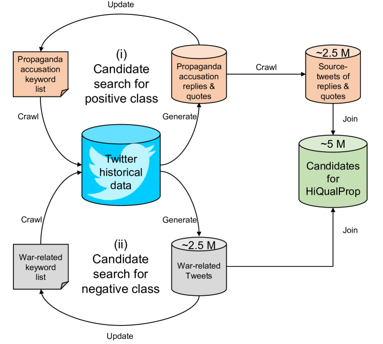
Figure 1: Data collection of candidate tweets for HQP.

(i) Candidate search for positive class ($D_{+}$): Analogous to Vijayaraghavan and Vosoughi (2022), we expect that propaganda on Twitter is often called out in replies or quotes (e.g., some users debunk propaganda as such). We thus access the Twitter Historical API and perform a keyword-based search. Specifically, we crawl replies and quotes that contain phrases (keywords) that may accuse the original tweet of propaganda, such as (“russian” $\land$ “propaganda”) or (“war” $\land$ “propaganda”). The full list is in Table A.1 in the supplements.

We create the list of search keywords through an iterative process: (1) In each iteration, the current list of keywords is used to filter for English-language replies and quotes from Twitter. (2) We then manually scan the most frequent words (including bi- and tri-grams) for phrases that can potentially qualify as propaganda accusations. (3) We add these to our list of keywords. We repeat the process for three iterations and use the final list of search keywords to retrieve our set of replies and quotes. Afterward, we crawl the corresponding source tweets, which resulted in $\sim$2.5 million candidates for $D_{+}$.

(ii) Candidates for negative class ($D_{-}$): To collect candidates for the negative class, we crawl a random sample of 2.5 million tweets that discuss the Russo-Ukrainian war but that have not necessarily been identified as propaganda through users. For this, we use a similar iterative procedure to generate a keyword list as for the positive class. However, we now perform a keyword search only for source tweets (but not for replies or quotes). Example keywords are (“russia” $\land$ “war”) and (“ukraine” $\land$ “war”). The complete list of search keywords is in Table A.2 in the supplements.

Postprocessing: We postprocess the candidates for both the positive class ($D_{+}$) and the negative class ($D_{-}$). Specifically, we filter out duplicates, non-English tweets, and very short tweets (i.e., fewer than 5 words). The resulting union of both postprocessed candidate sets contains $|D_{+}|+|D_{-}|\sim$3.2 million samples.

Unlike Vijayaraghavan and Vosoughi (2022), we do not perform weak labeling by simply assigning a label to a tweet depending on whether it is in $D_{+}$ or $D_{-}$, respectively. Instead, we generate high-quality labels through human annotation. This is motivated by our observation that many samples in $D_{+}$ cover the Russo-Ukrainian war but do not qualify as propaganda. Hence, weak labeling would lead to many false positives.

3.2 Boosted Sampling

We collect $N=$30,000$$ tweets from the postprocessed union of $D_{+}$ and $D_{-}$ for human annotation. We adopt boosted sampling Founta et al. (2018) as we observe that the majority of samples from the previous step cover ‘normal’ content and do not necessarily qualify as propaganda. Our research objective requires that there is a sufficient proportion of positive class labels in our dataset, since, otherwise, the dataset will not be useful for the research community. To address the class imbalance, we use weighted sampling. For this, we generate weights $w_{i}$ for each tweet as the inverse term frequency of potential propaganda-related phrases (e.g., “nobody talks about”), that is,

$$w_{i}= \,\frac{n_{i}}{\sum_{j=1}^{M}n_{j}},$$ (1)

where $n_{i}$ is the number of unique occurences of propaganda-related phrases and $M=|D_{+}|+|D_{-}|$. Here, we use the list of 189 potential propaganda phrases from Vijayaraghavan and Vosoughi (2022). As a result, our boosted sampling approach will increase the likelihood that actual propaganda content (true positives) is later annotated (rather than false positives).

3.3 Human Annotation

To annotate our data, we recruit human workers from Prolific (https://www.prolific.co/) to label the tweets as propagandistic or non-propagandistic. Workers are pre-selected according to strict criteria: residency in the UK/US, English as a first language; enrollment in an undergraduate, graduate, or doctoral degree; a minimum approval rate of 95%; and min. 500 completed submissions on Prolific. The annotation instructions are in Appendix B of the supplement.

Workers are asked to annotate two labels for each tweet. The first is a binary label (BL) to classify propagandistic vs. non-propagandistic content. The second is a propaganda-strategy label (PSL) aimed at capturing the context-related strategy behind propagandistic tweets. Therefore, if a tweet is annotated as propagandistic, the worker is asked to select one of four context-related propaganda strategies that are used in this tweet (thus giving PSL). The four propaganda strategies were carefully chosen after manually studying a sample of $2,000$ tweets and discussing different options with an expert team of propaganda researchers. Specifically, for PSL, workers have to decide whether the propagandistic tweet is designed to influence opinions (1) against Western countries, (2) against Ukraine, (3)  pro-Russian government, or (4) aimed at other countries.

Our annotation follows a batch procedure according to best practices Song et al. (2020), i.e., a pool of workers annotates a subset of the data to avoid fatigue. We thus split the dataset ($N=$30.000$$) into 300 batches with 100 tweets each. Each batch is annotated by two workers. Beforehand, we manually annotate 10 tweets of each batch with respect to BL to measure the quality of the annotations: If (a) a worker incorrectly labeled more than 20% of the internally annotated tweets or (b) the inter-annotator agreement between both workers has a Cohen’s kappa Cohen (1960) $\leq 0.4$, we discard the annotation and repeat the annotation for the batch. Overall, we had to discard and redo 7.5% of the batch annotations. When annotators disagreed on BL for individual tweets, we resolve the conflicts as follows: the BL is then re-annotated by randomly assigning it to one of the top 25 annotators. If there is disagreement on the PSL after resolving the disagreement on the BL, the final PSL is decided by the author team. The latter was the case for only 2.6% of the tweets. Altogether, this corroborates the reliability of our multi-annotator, multi-batch procedure for annotation.

We further crawled additional meta information about authors, which we report in Appendix F.

3.4 Dataset Statistics

Table 2 reports summary statistics for our HQP. Table 3 lists five example tweets and their corresponding labels, i.e., BL and PSL.

	Propaganda = true	Propaganda = false	Overall
Num. of tweets ($N$)	$4,610$	$25,390$	$30,000$
Avg. tweet length (in chars)	238.71	216.90	220.25
Num. of unique authors	$3,910$	$20,140$	$23,317$

Table 2: Summary statistics for HQP.

Tweet	BL	PSL
“STOP RUSSIAN AGGRESSION AGAINST #UKRAINE . @USER CLOSE THE SKY OVER UKRAINE ! EXCLUDE RUSSIA FROM THE @USER SECURITY COUNCIL ! #StopPutin #StopRussia HTTPURL”	False	—
“The Textile Worker microdistrict in Donetsk came under fire ! The Ukraine nazis dealt another blow to the residential quarter At least four civilians were killed on the spot . #UkraineRussiaWar #UkraineNazis #ZelenskyWarCriminal @USER @USER HTTPURL”	True	Against Ukraine
“The denazification of Ukraine continues . In Kherson , employees of the Russian Guard detained two accomplices of the Nazis . During the operation , the National Guard officers detained several leaders of neo-Nazi formations and accomplices of the SBU . HTTPURL HTTPURL”	True	Pro Russian government
“Western ‘leaders’ continue with their irrational drive toward WWIII . NATO is a criminal enterprise , an instrument of white power threat to global humanity . Join anti-NATO protests around the world . HTTPURL”	True	Against Western countries
“Chinese and Indian citizens must leave Ukraine because Ukraine is run by the Nazi / Zionist fascists since the coup d’etat of 2014 .”	True	Aimed at other countries

Table 3: Example tweets in our HQP dataset. BL is a binary label whether a tweet is propaganda or not. PSL is the propaganda strategy.

4 Methods

In our experiments, we follow state-of-the-art methods from the literature (see Sec. 2) to ensure the comparability of our results. To this end, we use a binary classification task (propaganda $=1$, otherwise $=0$). Results are reported as the average performance over five seperate runs. In each run, we divide the dataset into train (70%), val (10%), and test (20%) using a stratified shuffle split. All experiments are conducted on a Ubuntu 20.04 system, with 2.30 GHz Intel Xeon Silver 4316 CPU and two NVIDIA A100-PCIE-40GB GPUs.

4.1 Fine-Tuning PLMs

4.1.1 PLMs

We use the following PLMs in our experiments: BERT-large Devlin et al. (2019), RoBERTa-large Liu et al. (2019), and BERTweet-large Nguyen et al. (2020). The latter uses the pretraining procedure from RoBERTa but is tailored to English tweets in order to better handle social media content. We report implementation details in Appendix C.

4.1.2 Baselines

We compare the fine-tuning procedure on our high-quality labels vs. baselines that make use of weak labels. All evaluations are based on separate test splits of HQP with human verification.

$\bullet$ TWE: We fine-tune on weak labels of the public TWE dataset Wang et al. (2020).

$\bullet$ TWEETSPIN: The TWEETSPIN dataset with weak labels Vijayaraghavan and Vosoughi (2022) is not public, and we thus replicate the data collection procedure ($N=$3,223,867$$).

$\bullet$ HQP-weak: As an ablation study, we construct a dataset with weak labels based on our data collection procedure from HQP. Specifically, we map from our classification into $D_{+}$ and $D_{-}$. We generate $N=|\textsf{HQP}|$ samples so that the size is comparable to HQP. This allows us later to isolate the effect of the dataset size from the role of weak vs high-quality labels.

4.2 Prompt-Based Learning

For few-shot learning, we leverage state-of-the-art prompt-based learning Liu et al. (2023); Gao et al. (2021), which requires only a small set of labeled samples and thus reduces annotation costs. Prompt-based learning reformulates the downstream classification task to look more like the masked-language-model task the PLM was trained on. For example, for our task, each input sequence could be appended with a textual prompt, e.g., the propagandistic sequence “Ukraine is full of nazis.” is continued with the prompt “I stand with $\mathrm{[MASK]}$” (which gives the so-called template). Given a mapping of predefined label words to each class (via the so-called verbalizer), the masked language model predicts the probabilities of each label word to fill the $\mathrm{[MASK]}$ token and thereby the probabilities of each class. For our task, examples for label words could be “Russia” for the class of propaganda and “Ukraine” for the class of no propaganda. As a result, this introduces the task of prompt engineering, i.e., finding the most suitable template and verbalizer to solve the downstream task. In general, manual prompt engineering can be challenging, especially because the performance in the downstream task depends highly on the prompt Gao et al. (2021). In our work, we use a three-step procedure: (i) finding the best template, (ii) finding the best verbalizer, and (iii) prompt-based fine-tuning, as follows:

(i) Automatic template generation: Here, we use the LM-BFF procedure from Gao et al. (2021). We randomly sample $k^{\prime}$ positive and $k^{\prime}$ negative examples for training and validation, which thus requires $k=4\times k^{\prime}$ samples overall. We use the seq2seq PLM T5 Raffel et al. (2020) to generate template candidates. Given the training example and an initial verbalizer, T5 then generates a candidate template by filling the missing spans. We use beam search to generate a set of 100 candidate templates. Afterward, we fine-tune each template using the training examples and the downstream PLM. Finally, the best-performing template is chosen based on the performance on the val set.

(ii) Automatic verbalizer generation: We use the method from Gao et al. (2021) to generate the verbalizer (i.e., to map predictions to our label classes). For each class, we construct a set of 100 candidate tokens based on the conditional likelihood of the downstream PLM to fill the $\mathrm{[MASK]}$ token using the best-performing template from step (i). These candidates are fine-tuned and re-ranked to find the best candidate for each class with regard to the performance on the val set.

(iii) Prompt-based fine-tuning: We use the best template from step (i) and the best verbalizer from step (ii) to form our prompt. We fine-tune the downstream PLM with this prompt to create the final model for propaganda detection. We refer to the above model as LM-BFF.

In our LM-BFF implementation, we use the OpenPromt framework Ding et al. (2022). For template generation, we choose an initial verbalizer with label words “propaganda” (propaganda) and “truth” (no propaganda) and a cloze prompt format Liu et al. (2023). We choose RoBERTa-large Liu et al. (2019) as the underlying PLM due to its overall superior performance. We freeze the first 16 layers to control for overfitting and choose a learning rate of 4e$-$5. We train for a number of 50 epochs and choose the best checkpoint. We set the batch size depending on $k^{\prime}$; see Table 4. For all other hyper-parameters, we choose the same as those presented in Gao et al. (2021).

	$k^{\prime}=16$	$k^{\prime}=32$	$k^{\prime}=64$	$k^{\prime}=128$
Batch size	4	8	16	32

Table 4: Batch size of prompt-based learning for different numbers of overall samples ($k=4\times k^{\prime}$).

4.3 Extension of LM-BFF to Auxiliary-Task Prompting

We extend the above LM-BFF procedure for inductive learning and use both the BL and the PSL labels during prompting. The rationale behind this is three-fold: (1) We use information about the propaganda strategy and thus richer labels, which may improve performance. (2) Propaganda can be highly diverse, and, through the use of more granular labels, we can better capture heterogeneity. (3) The overall sample size remains low with only a minor increase in labeling costs. This is beneficial in practice when newly emerging propaganda narratives must be detected and there are thus only a few available samples.

To leverage both BL and PSL labels, we develop a custom architecture for auxiliary-task prompting, which we refer to as LM-BFF-AT. Specifically, we apply steps (i) to (iii) for our two labels BL and PSL, separately. This results in two different fine-tuned versions of the downstream PLM with different templates and verbalizers. To classify a given input text, we fuse verbalizer probabilities for each label into a classification head, which computes the final prediction. For the classification heads, we train an elastic net and a feed-forward neural network with one hidden layer on top of the verbalizer probabilities. The val set is used for hyper-parameter tuning. Hyper-parameter grids for the classification heads are reported in Appendix E. Note that our LM-BFF-AT approach uses two labels but can easily be generalized to $n$ labels.

5 Experiments

5.1 Discrepancy between Weak Labels vs. High-Quality Labels

RQ1: What is the discrepancy between weak labeling vs. human annotation?

We find a substantial discrepancy between the weak labels (from HQP-weak) and our high-quality labels (from human annotation). In fact, the overall agreement is only 41.0%. Hence, the majority of labels are thus different. Figure 2 shows the contingency table comparing weak and human annotation. Crucially, this supports our hypotheses that weak labels are noisy and thus often incorrect. This motivates our use of high-quality labels from human annotation in the following.

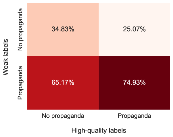
Figure 2: Contingency table comparing weak vs. high-quality labels.

5.2 Propopaganda Detection when using Weak vs. High-Quality Labels

RQ2: How well can state-of-the-art PLMs detect online propaganda when trained with weak labels vs. high-quality labels?

Table 5 compares the performance. For this, we vary the choice of the underlying PLM (BERT, RoBERTa, BERTweet) and what data is used for training (TWE, TWEETSPIN, HQP). We make the following observations: (1) The different PLMs reach a similar performance, which corroborates the robustness and reliability of our results. Recall that we intentionally chose state-of-the-art PLMs to allow for comparability when benchmarking the role of weak vs. high-quality labels. (2) Weak labels from the TWE dataset Wang et al. (2020) lead to an AUC similar to a random guess, while weak labels from the TWEETSPIN dataset reach an AUC of 64.03. (3) We use HQP-weak for an ablation study where we use the weak labels from our classification into $D_{+}$ and $D_{-}$ for training. We register an AUC of 56.79. (4) PLMs trained with high-quality labels perform best with an AUC of 92.25 (for BERTweet). Thereby, we achieve an improvement in AUC over best-performing weak labels (TWEETSPIN) of $\sim$44%. In sum, the performance gain must be exclusively attributed to the informativeness of high-quality labels (and not other characteristics of the dataset).

We further inspect weak vs. high-quality labels visually. For this, we plot the representation of the $\mathrm{[CLS]}$ tokens from HQP using $t$-SNE van der Maaten and Hinton (2008). As seen in Figure 3, the representations learned with high-quality labels (right plot) are more discriminatory for the true labels than that learned on weak labels (here: TWEETSPIN; left plot).

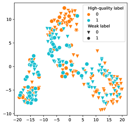
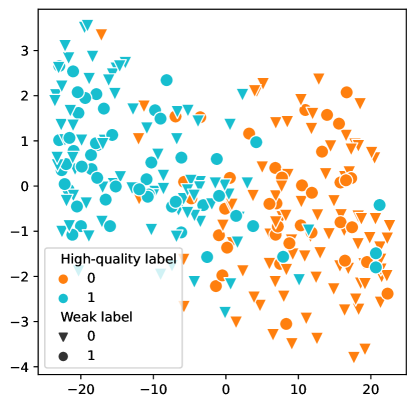
Figure 3: A $t$-SNE visualization showing the representations of the $\mathrm{[CLS]}$ tokens for BERTweet fine-tuned on TWEETSPIN labels (left) and high-quality labels (right). Evidently, representations learned with high-quality labels are more discriminatory than with weak labels for predictions on the test set .

	Precision			Recall			F1			AUC
Training data	BERT	RoBERTa	BERTweet	BERT	RoBERTa	BERTweet	BERT	RoBERTa	BERTweet	BERT	RoBERTa	BERTweet
TWE Wang et al. (2020)	14.86 (0.65)	14.67 (0.51)	14.75 (0.20)	46.04 (3.01)	45.71 (2.47)	53.47 (6.13)	22.46 (0.99)	22.20 (0.83)	23.08 (0.52)	47.93 (1.58)	48.63 (1.67)	47.22 (0.81)
TWEETSPIN Vijayaraghavan and Vosoughi (2022)	23.08 (1.51)	23.18 (1.11)	23.33 (1.25)	60.09 (1.87)	59.65 (1.48)	59.25 (1.85)	33.32 (1.54)	33.38 (1.36)	33.46 (1.46)	64.03 (1.05)	63.50 (1.06)	63.85 (1.41)
HQP-weak (weak labels on our HQP)	16.42 (0.17)	16.39 (0.31)	16.16 (0.18)	69.24 (1.38)	69.94 (3.03)	68.22 (2.64)	26.55 (0.30)	26.56 (0.61)	26.13 (0.43)	56.71 (0.99)	56.79 (2.07)	56.64 (0.76)
HQP (ours)	61.52 (5.77)	66.68 (2.30)	68.86 (2.37)	64.65 (3.83)	70.80 (2.85)	70.65 (2.52)	62.77 (1.92)	68.64 (1.80)	69.70 (1.31)	88.21 (0.62)	91.76 (0.62)	92.25 (0.80)
Stated: mean (SD).

Table 5: Results of propaganda detection for different PLMs trained on weak vs. high-quality labels.

5.3 Performance of Few-Shot Learning

RQ3: How much can few-shot learning reduce labeling costs for detecting online propaganda?

To reduce the costs of labeling, we further use few-short learning (see Figure 4). Here, we vary the overall number of labeled samples ($k=4\times k^{\prime}$). We compare the performance of prompt-based learning with LM-BFF (using only BL) vs. LM-BFF-AT (using BL and PSL).

Figure 4 compares the performance across the different values for $k^{\prime}$ and the prompt-based learning methods. Generally, a larger $k^{\prime}$ tends to improve the performance. For example, for $k^{\prime}=128$ and LM-BFF, we register a mean F1-score of 43.03 and a mean AUC of 79.74. As expected, this is lower than for fine-tuned PLMs but it is a promising finding since only 2.13% of the labeled examples are used for training and validation. Using LM-BFF-AT with an elastic net as the classification head consistently improves the performance of prompt-based learning across all $k^{\prime}$. For $k^{\prime}=128$, we achieve a 2.8% improvement in the F1-score (44.22) and a 0.7% improvement in AUC (80.27). On average, over all $k^{\prime}$, the improvement amounts to 1.25% for the F1-score and 0.51% for the AUC. Generally, the variant with an elastic net tends to be better than the variant with a neural network, likely due to the small size of the training sample.

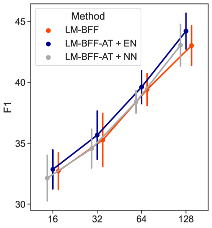
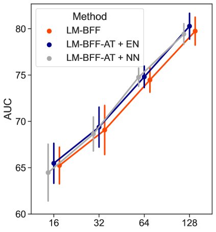
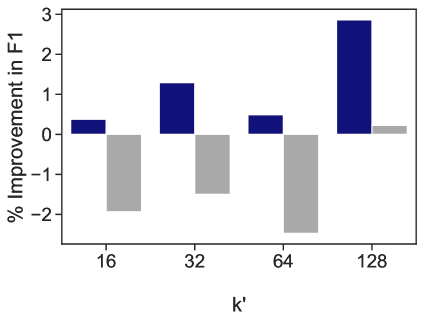
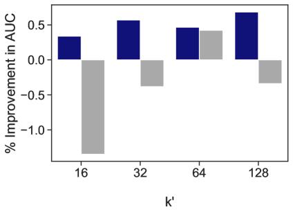
Figure 4: Results for prompt-based learning for LM-BFF vs. LM-BFF-AT (left: F1, right: AUC, top: absolute performance, bottom: %-improvement over LM-BFF). EN (NN) refers to the elastic net (neural net) classification head. $k^{\prime}$ refers to the number of examples sampled from each class for both training and validation, while $k=4\times k^{\prime}$ is the overall number of samples. Error bars denote the standard errors across 5 runs.

6 Discussion

We introduce HQP: the first dataset for online propaganda detection with human annotations. Our experiments further have direct implications for the NLP community.

$\bullet$ Implication 1: When identifying propaganda, there is a substantial discrepancy between weak labeling and human annotations. This pinpoints weaknesses in existing datasets for online propaganda detection Wang et al. (2020); Vijayaraghavan and Vosoughi (2022), since these make exclusive use of weak labeling. To this end, our work highlights the importance of human feedback for sensitive NLP tasks such as propaganda detection.

$\bullet$ Implication 2: High-quality labels are crucial to detect online propaganda. Our experiments are intentionally based on state-of-the-art PLMs to ensure reliability and comparability of our results. Generally, PLMs fail to detect propaganda when fine-tuned with weak labels. In contrast, there is a large improvement ($\sim$44%) when using high-quality labels.

$\bullet$ Implication 3: Few-shot learning can be an effective remedy to reduce the cost of human annotation of propaganda. To the best of our knowledge, our work is the first to adapt few-shot learning (via prompt-based learning) to propaganda detection. Interestingly, our performance is similar to that in related NLP tasks such as, e.g., detecting rumors Lin et al. (2023) and humor Li et al. (2023). Despite the challenging nature of our task, the performance of few-shot learning is promising. For example, only $k=64$ ($k^{\prime}=16$) high-quality annotated samples are needed to outperform propaganda detection with weak labels. For $k=512$ ($k^{\prime}=128$), we already achieve an improvement over weak labels of 24.54%.

7 Limitations

As with other works, ours is not free of limitation. First, there is no universal rule to determine what propaganda is and what not. Hence, the perception may vary across individuals. We address this by having our dataset annotated through multiple raters and showing raters a task description that includes a widely accepted definition of propaganda (see Smith, 2022). Second, we are further aware that PLMs may embed biases that are populated in downstream tasks. Hence, we call for careful use when deploying our methods in practice. Third, narratives that fall under the scope of propaganda may change over time. Hence, we recommend that both the dataset construction and the PLM fine-tuning is repeated regularly. To this end, we provide a cost-effective approach through few-shot learning.

8 Ethics Statement

Our dataset will benefit research on improving social media integrity. The construction of our dataset follows best-practice for ethical research Rivers and Lewis (2014). The dataset construction and usage was approved as ethically unproblematic by the ethics commission of the Faculty of Mathematics, Informatics and Statistics at LMU Munich (ethics approval number: EK-MIS-2023-160). In particular, our dataset contains only publicly available information. The privacy policy of Twitter warns users that their content can be viewed by the general public. Further, we respect the privacy of users and only report aggregate results throughout our paper. Although we believe the intended use of this work is largely positive, there exists potential for misuse (e.g., by propaganda campaigns to run adversarial attacks and develop techniques to avoid detection). To this end, we call for meaningful research by the NLP community to further improve social media integrity. Finally, we encourage careful use of our dataset, as it contains potentially offensive language and manipulative content, which lies in the nature of the task.

Appendix A Keywords for Dataset Construction

Table A.1 lists the keywords used in our dataset construction process to obtain candidate tweets for the positive class ($D_{+}$) via accusations in replies. Table A.2 shows the keywords that are used to collect candidate tweets for the negative class ($D_{-}$). Generally, keywords relevant to the positive class should mostly be terms that express accusations of propaganda, while keywords relevant to the negative class should be mostly terms that refer to general activities of the war. The keywords in both lists contain further results from our construction procedure in that we list the iteration in which they were added to the list.

Keywords ($D_{+}$)	Iteration
russia(n) $\land$ propaganda	1
russia(n) $\land$ propagandist	1
kremlin $\land$ propaganda	2
kremlin $\land$ propagandist	2
putinist(s)	2
putinism	2
russia(n) $\land$ lie(s)	3
war $\land$ propaganda	3
war $\land$ lie(s)	3
putin $\land$ propaganda	3
putin $\land$ propagandist	3
russia(n) $\land$ fake news	3

Table A.1: List of keywords used to get propaganda accusations and the corresponding iteration they were added to the keyword list. The $\land$-operator indicates that both keywords have to appear.

Keywords ($D_{-}$)	Iteration
russia $\land$ war	1
ukraine $\land$ war	1
#istandwithrussia	1
#istandwithputin	1
russian $\land$ war	2
ukrainian $\land$ war	2
#russianukrainianwar	2
#ukrainerussiawar	2
#standwithrussia	2
#standwithputin	2
#russia	2
#russiaukraine	2
#ukraine	2
putin $\land$ war	3
#putin	3
#lavrov	3
#zakharova	3
#nato	3
#donbass	3
#mariupol	3

Table A.2: List of keywords used to get war-related tweets and the corresponding iteration they were added to the keyword list. The $\land$-operator indicates that both keywords have to appear.

Appendix B Annotation Instructions

Figure B.1 shows the instructions of batch annotations we present to the workers on Prolific (https://www.prolific.co/). We follow best practices Song et al. (2020). That is, we provide a detailed and comprehensible description of the task, a precise definition of the labels, and a transparent disclosure that we use attention checks.

Given the complexity and subjective nature of propaganda, we put great emphasis on providing meaningful and precise instructions for annotation. Therefore, the final instructions in Figure B.1 are a result of several iterations of improvement, each followed by an internal discussion and analysis. In each iteration, we had three workers from Prolific annotate a random sample of 100 tweets using the current version of the instructions. We analyzed the resulting annotations and focused on the samples with disagreement. We then aimed to address the corresponding issues in the next update of our instructions. In each iteration, we calculated the inter-annotator agreement using Krippendorff’s alpha Krippendorff et al. (2016) and stopped iterating after surpassing an agreement of 0.8 for the first time. As a result, we updated the instructions three times.

We also followed best practices and applied attention checks. Participants failing the attention checks were removed, and the annotation was repeated.

Figure B.1: Instructions for annotators.

Appendix C Implemenation Details for Full Fine-tuning

For fine-tuning, we add a linear layer to the hidden representation of the $\mathrm{[CLS]}$ token. The PLMs are then fine-tuned using the transformer framework from Huggingface Wolf et al. (2020). We set the maximum sequence length to 128. We use a training batch size of 32 and a learning rate of 4e-5. We freeze the first 16 layers of the PLMs. For BERT-large and RoBERTa-large, we add emoji-tokens to the vocabulary due to their frequent and meaningful use in social media. Weight updates are performed using the AdamW-optimizer Loshchilov and Hutter (2019). We fine-tune for a maximum number of 5 epochs. We validate the performance every 500 steps for fine-tuning with TWEETSPIN and every 50 steps otherwise. Early stopping is used when the loss on the validation set does not decrease for more than 5 validation steps.

Appendix D Evaluation of the Auxiliary Task in LM-BFF-AT

In Table D.1, we report the performance of the auxiliary task in LM-BFF-AT, i.e., the performance of prompt-based learning using PSL.

k’	Weighted Precision	Weighted Recall	Weighted F1
16	75.06 (2.54)	66.17 (6.81)	69.84 (4.02)
32	75.6 (1.21)	64.93 (10.73)	68.75 (7.48)
64	77.46 (2.19)	75.31 (4.45)	76.13 (2.15)
128	77.18 (3.45)	74.39 (3.87)	75.41 (1.86)
Stated: mean (SD).

Table D.1: Evaluation results for the auxiliary task of prompt-based learning using PSL on HQP.

Appendix E Hyper-Parameters for Classification Heads of LM-BFF-AT

For our extension of the LM-BFF method, namely LM-BFF-AT, we perform hyper-parameter tuning using grid search for the two classification heads, i.e., the elastic net and the neural net. The tuning grids are reported in Table E.1. We implement the elastic net using Python’s scikit-learn module. The neural net is implemented using PyTorch.

Classification head	Hyper-parameter	Grid
Elastic net	Cost	{0.1, 0.25, 0.5, 1, 2, 4, 8}
	L1-ratio	{0.1, 0.15, 0.2, 0.25, 0.3, 0.35}
Neural net	Dropout	{0.2, 0.4, 0.6}
	Learning rate	{0.001, 0.01, 0.02}
	Batch size	{2, 4, 8, 16}
	Neurons in hidden layer	$\mathit{input\_dim}*${0.5, 1, 1.5, 2}

Table E.1: Grids for hyper-parameter tuning of the two classification heads for prompt-based learning with LM-BFF-AT. The cost $C=\frac{1}{\lambda}$ is the inverse of the regularization strength. L1-ratio is the elastic net mixing parameter (i.e., is equivalent to only using an L2-penalty (or L1-penalty) for L1-ratio$=0$ (or L1-ratio$=1$) and mixes both for $0<$ L1-ratio $<1$). Here, $\mathit{input\_dim}$ is the number of input features and therefore depends on whether only probabilities from the verbalizers or also author representations are used.

Appendix F Propaganda Detection with Additional Meta Information

We extend our propaganda detection so that we not only use the content but the additional meta information (i.e., author features and pinned-tweet features) for propaganda detection.

F.1 Data Enrichment

We enrich HQP with additional meta information from the social network. Here, we use a comprehensive set of author features (e.g., number of followers, account age, verified status) and pinned-tweet features (e.g., tweet age, number of likes, number of retweets). Our data further includes the profile description of authors using embeddings from SBERT Reimers and Gurevych (2019). We choose SBERT due to its strength in capturing meaningful representations from short text Reimers and Gurevych (2019). A few tweets corresponded to authors whose accounts were already deleted, which reduces our dataset to the final size of $N=$29,596$$. We note that for fair benchmarking we used the dataset of size $N=$29,596$$ for all experiments. The full list of features is in Section F.2.

F.2 Summary Statistics

	Propaganda = true		Propaganda = false
	Mean	Median	Mean	Median
Verified (=1; not=0)	0.09	0	0.19	0
#Followers	102784.72	513	595308.01	13405
#Following	1927.58	530.5	3237.82	786
#Tweets	37780.17	11123.5	64060.48	16811
#Listed∗	633.36	5	2449.10	11
Account age (in days)	2272.17	1938	2763.28	2895
#Followers divided by Account age	28.05	0.37	161.74	0.71
#Following divided by Account age	1.19	0.34	1.48	0.34
#Tweets divided by Account age	19.34	7.915	25.76	8.58
∗Number of Twitter lists (i.e., a curated group of accounts) comprising the account of the author.

Table F.1: Summary statistics of author features in HQP.

	Propaganda = true		Propaganda = false
	Mean	Median	Mean	Median
Account age (in days)	365.30	198	366.82	170
#Retweets	573.12	13	1051.95	17
#Replies	251.85	6	416.71	7
#Likes	2232.50	39	4336.85	62
#Quotes	70.19	2	131.85	2
#Retweets divided by account age	16.70	0.08	30.49	0.14
#Replies divided by account age	5.09	0.03	11.95	0.05
#Likes divided by account age	59.17	0.25	111.47	0.5
#Quotes divided by account age	1.14	0.01	3.18	0.01

Table F.2: Summary statistics for pinned-tweet features of authors in HQP.

Table F.1 reports summary statistics of the author features for HQP. We compare mean and standard deviation separately for both propagandistic and non-propagandistic content. In line with previous findings Geissler et al. (2022), we find that authors of propagandistic content are, on average, less often verified, have fewer followers and tweets, and are characterized by a younger account age. Table F.2 reports summary statistics for the pinned-tweet features of the authors in HQP.

F.3 Adaptation of Methods

(i) Full fine-tuning: We modify the classification head so that we perform full fine-tuning with author and pinned-tweet features. The self-description of tweet authors is encoded into a 768-dimensional vector using SBERT. We normalize the numerical features from Table F.1 and Table F.2 and append them to the self-description vector to get an author representation. We concatenate the hidden representation of the $\mathrm{[CLS]}$ token generated by the PLM and the author representation and again feed them to a linear layer. The fine-tuning procedure and the hyper-parameters are identical to those described in Section 4.1.

(ii) Prompt-based learning: We create the same author representation as in (i). Here, we concatenate the author representation with the verbalizer probabilities for both BL and PSL and again feed them to a classification head as in LM-BFF-AT. The prompt-based learning procedure is identical to that in Section 4.2, i.e., we select the optimal template and verbalizer from each run in Section 5.3. The tuning grids for hyper-parameter tuning for the two classification heads are identical to those in Table E.1.

F.4 Results

Table F.3 reports the prediction performance when additionally using author features. Values are in bold if the model that uses additional author and pinned-tweet features outperforms the counterpart without author features. Overall, we observe a tendency that the results improve when additionally using author features. This tendency is seen for both full fine-tuning and prompt-based learning. However, the performance gain from using the content is larger than the performance gain from using author features. This can be expected as propaganda spreaders typically do not explicitly disclose their manipulative intention but instead aim to deceive users.

	PLM	P	R	F1	AUC
(i) Full fine-tuning	BERT	64.58 (3.19)	62.40 (1.94)	63.42 (1.64)	88.54 (0.81)
	RoBERTa	67.61 (3.05)	69.59 (3.02)	68.52 (2.04)	91.37 (1.02)
	BERTweet	67.06 (3.39)	72.68 (1.54)	69.71 (1.79)	92.06 (0.86)
	$k^{\prime}$	P	R	F1	AUC
(ii) Prompt-based learning	16	22.38 (3.37)	64.94 (9.79)	32.98 (3.49)	64.99 (4.16)
	32	24.75 (6.24)	65.16 (3.6)	35.70 (4.16)	69.29 (4.48)
	64	27.73 (2.80)	70.72 (4.07)	39.74 (2.88)	74.88 (2.21)
	128	30.81 (2.86)	76.38 (1.52)	43.86 (3.02)	79.46 (2.89)
Stated: mean (SD). P: precision. R: recall.

Table F.3: Evaluation results of (i) full fine-tuning and (ii) prompt-based learning on HQP while incorporating author and pinned-tweet features. Results are shown in bold if the performance with author and pinned-tweet features is better than the performance without author features.

References

- Badjatiya et al. (2017) Pinkesh Badjatiya, Shashank Gupta, Manish Gupta, and Vasudeva Varma. 2017. Deep learning for hate speech detection in tweets. In WWW Companion.