Revisiting constraints on the photon rest mass with cosmological fast radio bursts

Abstract

Fast radio bursts (FRBs) have been suggested as an excellent celestial laboratory for testing the zero-mass hypothesis of the photon. In this work, we use the dispersion measure (DM)–redshift measurements of 23 localized FRBs to revisit the photon rest mass $m_{\gamma}$. As an improvement over previous studies, here we take into account the more realistic probability distributions of DMs contributed by the FRB host galaxy and intergalactic medium (IGM) from the IllustrisTNG simulation. To better account for the systematic uncertainty induced by the choices of priors of cosmological parameters, we also combine the FRB data with the cosmic microwave background data, the baryon acoustic oscillation data, and type Ia supernova data to constrain the cosmological parameters and $m_{\gamma}$ simultaneously. We derive a new upper limit of $m_{\gamma}\leq 3.8\times 10^{-51}\;\rm{kg}$, or equivalently $m_{\gamma}\leq 2.1\times 10^{-15}\,\rm{eV/c^{2}}$ ($m_{\gamma}\leq 7.2\times 10^{-51}\,\rm{kg}$, or equivalently $m_{\gamma}\leq 4.0\times 10^{-15}\,\rm{eV/c^{2}}$) at $1\sigma$ ($2\sigma$) confidence level. Meanwhile, our analysis can also lead to a reasonable estimation for the IGM baryon fraction $f_{\rm IGM}=0.873^{+0.061}_{-0.050}$. With the number increment of localized FRBs, the constraints on both $m_{\gamma}$ and $f_{\rm IGM}$ will be further improved. A caveat of constraining $m_{\gamma}$ within the context of the standard $\Lambda$CDM cosmological model is also discussed.

1 Introduction

It is a widely accepted consensus in modern physics that the rest mass of the photon should be exactly zero. However, several theories suggest otherwise, such as the de Broglie-Proca theory [1, 2], the model of massive photons as dark energy [3], massive photons within an alternative gravity scenario [4], and other new ideas in classical electrodynamics with massive photons [5, 6, 7]. Testing the correctness of the photon zero-mass hypothesis has emerged as an attractive task in modern physics, as it could potentially shed light on these alternative theories.

Some measurable effects have been predicted when photons have nonzero mass. The photon rest mass can then be effectively constrained by seeking such effects [8, 9, 10, 11, 12, 13, 14]. Over the last few decades, a number of methods have been proposed to constrain the photon mass, including tests of Coulomb’s inverse square law [15], tests of Ampère’s law [16], experiments of Cavendish torsion balance [17], exploration on the gravitational deflection of electromagnetic waves [9, 18], measurement of Jupiter’s magnetic field [19], analysis of cosmic magnetic field vector potential [20, 21], measurement of redshift/blueshift associated with alternative fits of the Hubble diagram of type Ia supernovae (SNe Ia; [7, 22]), and so on.

The most direct way to determine the photon mass or, more precisely, place an upper bound on the photon mass is to measure the frequency dependence in the velocity of light. When laboratory experiments suffer from limitations, astrophysical observations afford excellent conditions for higher precision measurements on the relative velocities of electromagnetic waves with different frequencies [23, 24, 25, 26, 27, 28, 29, 30, 31, 32, 33, 34, 35, 36, 37, 38]. If the photon rest mass is nonzero, then the speed of light in vacuum is no longer a constant but is a function of frequency. Two photons with different frequencies, if emitted simultaneously from the same astrophysical source and traveling through the same distance, would thus be observed at different times (see Ref. [39] for a recent review). As a new kind of millisecond radio transient occurring at cosmological distances, fast radio bursts (FRBs) offer the current best astrophysical laboratory for testing the photon mass through the dispersion method [23, 24, 25, 26, 27, 28, 29, 30, 31].

While stringent photon mass limits from FRBs have been obtained, some obstacles to the pace of advance remain. The dispersion measure (DM) contribution from the FRB host galaxy ($\mathrm{DM_{host}}$) is not well known, and it also degenerates with the DM contributed by the intergalactic medium (IGM; $\rm{DM_{IGM}}$). Due to the large IGM fluctuation, $\rm{DM_{IGM}}$ at a given redshift can vary significantly along different lines of sight [40]. In most previous works, $\mathrm{DM_{host}}$ for all FRB host galaxies was treated as an unknown constant, and a global systematic uncertainty was introduced to account for the diversity of host galaxy contribution and the large IGM fluctuation. This treatment amounts to assuming that the probability distributions of $\rm{DM_{IGM}}$ and $\mathrm{DM_{host}}$ are symmetric. However, numerical simulations show that the distributions of $\rm{DM_{IGM}}$ and $\mathrm{DM_{host}}$ are asymmetric and have a significant positive skew [41, 42, 43]. A more appropriate way to model $\rm{DM_{IGM}}$ and $\mathrm{DM_{host}}$ is thus required in FRB photon mass limits. Recently, Lin et al. [31] constrained the photon mass by considering the more realistic non-Gaussian distributions for $\rm{DM_{IGM}}$ and $\mathrm{DM_{host}}$, but ignoring the degeneracy between the photon mass and cosmological parameters. It should be emphasized that just relying on the FRB data is difficult to constrain the photon mass and cosmological parameters simultaneously, even with only cosmological parameters [44]. All previous works neglected the parameter degeneracy and set the cosmological parameters as fixed values. In such cases, the uncertainties of cosmological parameters might affect the constraints on the photon mass.

In this paper, we use the most up-to-date sample of localized FRBs to revisit the photon mass, by properly taking into account the accurate probability distributions of $\rm{DM_{IGM}}$ and $\mathrm{DM_{host}}$ derived from the IllustrisTNG simulation [42, 43]. Compared with previous works, in addition to the photon mass, the cosmological parameters as well as the baryon fraction in the IGM ($f_{\rm IGM}$) are also treated as free parameters. In order to break the parameter degeneracy, we combine the DM–$z$ measurements from FRBs with the cosmic microwave background (CMB) data from the latest Planck release [45, 46], the baryon acoustic oscillation (BAO) data [47], and 1048 Pantheon SN Ia data [48]. With the observational data, we constrain the photon mass and model parameters simultaneously.

This paper is organized as follows. In Section 2, we introduce a theoretical framework for estimating the probability distributions of $\mathrm{DM_{IGM}}$ and $\mathrm{DM_{host}}$, and a method to constrain the photon mass. The observational data and the resulting constraints on the photon mass and other model parameters are presented in Section 3. Finally, discussion and conclusions are drawn in Section 4.

2 Theoretical Framework

2.1 Dispersion from the Plasma

FRB signals at low frequencies would travel through the plasma slower than those at high frequencies. This phenomenon is known as the dispersion effect. The arrival time difference between low- and high-frequency photons propagating from a distant source to the observer is described as [49, 37, 28]

$$\Delta t_{\rm{DM}}=\frac{e^{2}}{8\pi^{2}m_{e}\epsilon_{0}c}\left(\nu_{l}^{-2}-\nu_{h}^{-2}\right)\mathrm{DM_{astro}}\;,$$ (2.1)

where $e$ and $m_{e}$ are the charge and mass of an electron, respectively, $\epsilon_{0}$ is the permittivity of vacuum, $c$ is the speed of light in vacuum, and $\nu_{l}$ and $\nu_{h}$ are the low and high frequencies of photons, respectively. Here $\mathrm{DM_{astro}}$ is the DM contribution from the plasma, which is defined as the integral of electron number density $n_{e}$ along the line of sight.

For an extragalactic FRB, the $\mathrm{DM_{astro}}$ can be divided into four main components:

$$\mathrm{DM_{astro}}=\mathrm{DM_{ISM}^{MW}}+\mathrm{DM_{halo}^{MW}}+\mathrm{DM_{IGM}}(z)+\frac{\mathrm{DM_{host,0}}}{1+z}\;,$$ (2.2)

where $\mathrm{DM_{ISM}^{MW}}$ and $\mathrm{DM_{halo}^{MW}}$ are contributed by the Milky Way’s interstellar medium (ISM) and halo, respectively. $\mathrm{DM_{IGM}}$ represents the IGM portion of DM, and $\mathrm{DM_{host,0}}$ is the DM contribution from the host galaxy. The $(1+z)$ factor corrects the local $\mathrm{DM_{host,0}}$ to the measured value $\mathrm{DM_{host}}$ [50].

The average $\mathrm{DM_{IGM}}$ is related to the cosmological distance scale and the ionization fractions of intergalactic hydrogen and helium. If both hydrogen and helium are completely ionized (valid below $z\sim 3$), then it can be calculated as [51, 52]

$$\left\langle\mathrm{DM}_{\mathrm{IGM}}(z)\right\rangle=\frac{21c\Omega_{b0}H_{0}f_{\mathrm{IGM}}}{64\pi Gm_{p}}H_{e}(z)\;,$$ (2.3)

where $H_{0}$ is the Hubble constant, $m_{p}$ is the proton mass, $G$ is the gravitational constant, $\Omega_{b0}$ is the present-day baryon density parameter, and $f_{\mathrm{IGM}}$ is the baryon fraction in the IGM. Although some numerical simulations and observations suggested that $f_{\mathrm{IGM}}$ is slowly evolving with redshift [53, 54, 55], a recent study indicated that such evidence is absent in the relatively small amount of FRB data [56]. Here we thus consider $f_{\mathrm{IGM}}$ as a constant. Adopting the flat $\Lambda$CDM cosmological model, the dimensionless redshift function $H_{e}(z)$ is given by

$$H_{e}(z)=\int_{0}^{z}\frac{1+z^{\prime}}{\sqrt{\Omega_{m0}(1+z^{\prime})^{3}+1-\Omega_{m0}}}dz^{\prime}\;,$$ (2.4)

where $\Omega_{m0}$ is the matter density parameter.

2.2 Dispersion from a Nonzero Photon Mass

The relative time delay between low- and high-frequency photons caused by the nonzero photon mass can be approximatively expressed as [23, 28]

$$\Delta t_{m_{\gamma}}=\frac{1}{2H_{0}}\left(\frac{m_{\gamma}c^{2}}{h}\right)^{2}\left(\nu_{l}^{-2}-\nu_{h}^{-2}\right)H_{\gamma}(z)\;,$$ (2.5)

where $h$ is the Planck constant, and $H_{\gamma}(z)$ is the other dimensionless function,

$$H_{\gamma}(z)=\int_{0}^{z}\frac{(1+z^{\prime})^{-2}}{\sqrt{\Omega_{m0}(1+z^{\prime})^{3}+1-\Omega_{m0}}}dz^{\prime}\;.$$ (2.6)

It is evident that $\Delta t_{\rm{DM}}$ and $\Delta t_{m_{\gamma}}$ have a similar frequency dependency ($\Delta t\propto\nu^{-2}$). Thus, we can define an “effective DM” arises from a nonzero photon mass [26],

$$\mathrm{DM}_{\gamma}(z)=\frac{4\pi^{2}m_{e}\epsilon_{0}c^{5}}{h^{2}e^{2}}\frac{H_{\gamma}(z)}{H_{0}}m_{\gamma}^{2}\;.$$ (2.7)

Comparing the two redshift functions $H_{e}(z)$ and $H_{\gamma}(z)$, one can see that the DM contributions from the IGM and a nonzero photon mass ($\mathrm{DM_{IGM}}$ and $\mathrm{DM}_{\gamma}$) have different redshift dependencies. Therefore, the dispersion degeneracy between $\mathrm{DM_{IGM}}$ and $\mathrm{DM}_{\gamma}$ could in principle be broken when a large redshift measurements of FRBs are available [24, 25, 49, 26, 28].

2.3 Methodology

Suppose that the nonzero photon mass effect exists, the observed DM extracted from the dynamical spectrum of an FRB should include both $\mathrm{DM_{astro}}$ and $\mathrm{DM}_{\gamma}$, i.e.,

$$\mathrm{DM_{obs}}=\mathrm{DM_{astro}}+\mathrm{DM}_{\gamma}\,.$$ (2.8)

If the different DM contributions in Equation (2.2) can be estimated properly, then we can effectively identify $\mathrm{DM}_{\gamma}$ from $\mathrm{DM_{obs}}$, thereby providing a constraint on the photon mass $m_{\gamma}$.

The DM due to the Milky Way’s ISM, $\mathrm{DM_{ISM}^{MW}}$, can be well estimated based on the Galactic electron density models. Here we adopt the NE2001 model to estimate $\mathrm{DM_{ISM}^{MW}}$ [57]. The $\mathrm{DM_{halo}^{MW}}$ term contributed by the Milky Way’s halo is not well known but is expected to be 50–80 $\mathrm{pc\;cm^{-3}}$ [58]. According to this estimation, we consider a Gaussian prior on $\mathrm{DM_{halo}^{MW}}=65\pm 15$ $\mathrm{pc\;cm^{-3}}$ [59].

For a well-localized FRB, the average $\langle\mathrm{DM}_{\mathrm{IGM}}\rangle$ can be calculated using Equation (2.3). However, due to the density fluctuations of large-scale structure, the real value of $\mathrm{DM}_{\mathrm{IGM}}$ would vary significantly around the average. Theoretical treatments of the IGM and galaxy halos show that the probability distribution for $\mathrm{DM}_{\mathrm{IGM}}$ can be well modelled by a quasi-Gaussian function with a long tail [40, 58, 41],

$$P_{\mathrm{IGM}}\left({\rm DM_{IGM}}\right)=A\Delta^{-\beta}\exp\left[-\frac{\left(\Delta^{-\alpha}-C_{0}\right)^{2}}{2\alpha^{2}\sigma_{\mathrm{DM}}^{2}}\right],\;\Delta>0\;,$$ (2.9)

where $\Delta\equiv\mathrm{DM}_{\mathrm{IGM}}/\langle\mathrm{DM_{IGM}}\rangle$, $A$ is a normalization coefficient, $\sigma_{\mathrm{DM}}$ is an effective deviation arises from the inhomogeneities of the IGM, and $C_{0}$ is chosen such that the average $\left\langle\Delta\right\rangle=1$. $\alpha$ and $\beta$ are two indices related to profile scales, which are set to be $\alpha=\beta=3$ [41]. Using the state-of-the-art IllustrisTNG simulation [60], Zhang et al. [43] estimated the best-fits of $A$, $\sigma_{\mathrm{DM}}$, and $C_{0}$ at different redshifts. Since the $\mathrm{DM}_{\mathrm{IGM}}$ distributions derived from the IllustrisTNG simulation are given in discrete redshifts [43], we extrapolate their parameter values to the redshifts of our localized FRBs through the cubic spline interpolation method.

The host contribution $\mathrm{DM_{host}}$ is hard to determine, and may change significantly from hosts to hosts. Based on the observations of FRB hosts, Zhang et al. [42] selected plenty of simulated galaxies with similar properties to observed ones from the IllustrisTNG simulation for calculating the $\mathrm{DM_{host}}$ distribution of FRBs. It has been shown that the probability distribution of $\mathrm{DM_{host}}$ follows a lognormal function [41, 42],

$$P_{\mathrm{host}}\left(\mathrm{DM}_{\mathrm{host}}\right)=\frac{1}{\sqrt{2\pi}\mathrm{DM}_{\mathrm{host}}\sigma_{\mathrm{host}}}\exp\left[-\frac{\left(\ln\mathrm{DM}_{\mathrm{host}}-\mu_{\mathrm{host}}\right)^{2}}{2\sigma_{\mathrm{host}}^{2}}\right]\,,$$ (2.10)

where $\mu_{\mathrm{host}}$ and $\sigma_{\mathrm{host}}$ denote the mean and standard deviation of $\ln\mathrm{DM}_{\mathrm{host}}$, respectively. According to the properties of their host galaxies, Zhang et al. [42] divided FRBs into three types. For each type, the best-fitting values of $\mu_{\mathrm{host}}$ and $\sigma_{\mathrm{host}}$ at different redshifts are available in their article. In our analysis, we use their results to get $\mu_{\mathrm{host}}$ and $\sigma_{\mathrm{host}}$ at any given redshifts by cubic spline interpolation. It is obvious that different host types correspond to different $\mathrm{DM_{host}}$ distributions [42]. While Lin et al. [31] used the same $\mathrm{DM_{host}}$ distribution to describe all FRB hosts.

If a sample of localized FRBs is observed, the joint likelihood function is given by [41]

$$\mathcal{L}_{\rm FRB}=\prod_{i=1}^{N_{\mathrm{FRBs}}}P_{i}\left(\mathrm{DM}_{\mathrm{E},i}\right),$$ (2.11)

where $N_{\mathrm{FRBs}}$ is the number of available FRBs and $P_{i}\left(\mathrm{DM}_{\mathrm{E},i}\right)$ represents the probability of the observed $\mathrm{DM_{obs}}$ corrected for our Galaxy:

$$\mathrm{DM_{E}}\equiv\mathrm{DM_{obs}}-\mathrm{DM_{ISM}^{MW}}-\mathrm{DM_{halo}^{MW}}=\mathrm{DM_{IGM}}+\mathrm{DM_{host}}+\mathrm{DM_{\gamma}}\;.$$ (2.12)

For an FRB at a given $z_{i}$, we can calculate $P_{i}(\mathrm{DM}_{\mathrm{E},i})$ through:

$$\begin{split}P_{i}\left(\mathrm{DM}_{\mathrm{E},i}\right)&=\int_{0}^{\mathrm{DM}_{\mathrm{E},i}-\mathrm{DM_{\gamma}}}P_{\text{host}}\left(\mathrm{DM}_{\mathrm{host}}\right)\\ &\times P_{\mathrm{IGM}}\left(\mathrm{DM}_{\mathrm{E},i}-\mathrm{DM}_{\mathrm{host}}-\mathrm{DM_{\gamma}}\right)\mathrm{dDM}_{\mathrm{host}}\;,\end{split}$$ (2.13)

where $P_{\mathrm{IGM}}(\mathrm{DM_{IGM}})$ and $P_{\text{host}}(\mathrm{DM_{host}})$ are the probability density functions for $\mathrm{DM_{IGM}}$ and $\mathrm{DM_{host}}$, respectively.

Table 1: Properties of 23 FRBs with redshift measurements.

Name	Redshift	$\mathrm{DM_{obs}}$	$\mathrm{DM_{ISM}^{MW}}$	References
		$(\mathrm{pc\,cm^{-3}})$	$(\mathrm{pc\,cm^{-3}})$
FRB 121102	0.19273	557	188.0	1
FRB 180301	0.3304	536	152.0	2
FRB 180916	0.0337	348.76	200.0	3
FRB 180924	0.3214	361.42	40.5	4
FRB 181112	0.4755	589.27	102.0	5
FRB 190102	0.291	363.6	57.3	6
FRB 190523	0.66	760.8	37.0	7
FRB 190608	0.1178	338.7	37.2	8
FRB 190611	0.378	321.4	57.83	9
FRB 190614	0.6	959.2	83.5	10
FRB 190711	0.522	593.1	56.4	9
FRB 190714	0.2365	504	38.0	9
FRB 191001	0.234	506.92	44.7	9
FRB 191228	0.2432	297.5	33.0	2
FRB 200430	0.16	380.1	27.0	9
FRB 200906	0.3688	577.8	36.0	2
FRB 201124	0.098	413.52	123.2	11
FRB 210117	0.2145	730	34.4	12
FRB 210320	0.27970	384.8	42	12
FRB 210807	0.12927	251.9	121.2	12
FRB 211127	0.0469	234.83	42.5	12
FRB 211212	0.0715	206	27.1	12
FRB 220610A	1.016	1457.624	31	13

References: (1) Chatterjee et al. (2017) [61]; (2) Bhandari et al. (2022) [62]; (3) Marcote et al. (2020) [63]; (4) Bannister et al. (2019) [64]; (5) Prochaska et al. (2019) [65]; (6) Bhandari et al. (2020) [66]; (7) Ravi et al. (2019) [67]; (8) Chittidi et al. (2021) [68]; (9) Heintz et al. (2020) [69]; (10) Law et al. (2020) [70]; (11) Ravi et al. (2022) [71]; (12) James et al. (2022) [72]; (13) Ryder et al. (2022) [73].

3 Data and Results

Currently, 26 extragalactic FRBs have already been localized. FRB 200110E is the nearest one ($D\sim 3.6$ Mpc), and its redshift is dominated by the peculiar velocity, rather than by the Hubble flow. It thus has a negative spectroscopic redshift $z=-0.0001$ [74, 75]. The observed $\mathrm{DM_{obs}}$ value of FRB 181030 is so small ($\sim 103.396$ $\mathrm{pc\;cm^{-3}}$; [76]) that it would be reduced to a negative value after subtracting $\mathrm{DM_{ISM}^{MW}}$ and $\mathrm{DM_{halo}^{MW}}$. That is, the integral upper limit ($\mathrm{DM_{E}}-\mathrm{DM_{\gamma}}=\mathrm{DM_{obs}}-\mathrm{DM_{ISM}^{MW}}-\mathrm{DM_{halo}^{MW}}$, where its $\mathrm{DM_{ISM}^{MW}}$ is 40.16 $\mathrm{pc\;cm^{-3}}$ and $\mathrm{DM_{halo}^{MW}}$ is set to be $65\pm 15\;\mathrm{pc\;cm^{-3}}$) in Equation (2.13) would become negative. Due to an enormously large DM contributed by its host galaxy, FRB 190520B deviates significantly from the expected $\mathrm{DM_{IGM}}$–$z$ relation [77]. Therefore, we exclude these three FRBs. The remaining 23 FRBs are then used for the following analysis. Table 1 lists the redshifts, $\mathrm{DM_{obs}}$, and $\mathrm{DM_{ISM}^{MW}}$ of these 23 localized FRBs.

Table 2: The $1\sigma$ constraints on all parameters. Both the $1\sigma$ and $2\sigma$ upper limits on the photon mass $m_{\gamma}$ are displayed.

Parameters	Values
$m_{\gamma}\;[10^{-51}\,{\rm kg}]$	$\leq 3.8\;(1\sigma)$
	$\leq 7.2\;(2\sigma)$
$f_{\rm IGM}$	$0.873^{+0.061}_{-0.050}$
$\mathrm{DM_{halo}^{MW}}\;[\mathrm{pc\;cm^{-3}}]$	$\leq 60.1$
$\Omega_{m0}$	$0.309^{+0.005}_{-0.006}$
$\Omega_{b0}h^{2}$	$0.02246\pm 0.00014$
$H_{0}\;[{\rm km\,s^{-1}\,Mpc^{-1}}]$	$67.77\pm 0.43$
$M_{B}$	$-19.415\pm 0.012$

In order to break the degeneracies among model parameters, we combine FRB data with up-to-date cosmological probe compilations, including CMB, BAO, and SNe Ia. For the CMB data, we use the derived acoustic scale $l_{A}$, shift parameter $R$, and $\Omega_{b0}h^{2}$ from the latest Planck analysis of the CMB (TT, TE, EE $+$ lowE) [45, 46]. For BAO, we adopt a combination of 11 BAO measurements from Ref. [47]. For the SN sample, we use the 1048 Pantheon SNe Ia [48]. Please see Ref. [56] for more details on the exact compilations and the likelihood functions of these cosmological probes. The final log-likelihood is thus a sum of the separated likelihoods of FRBs, CMB, BAO, and SNe Ia:

$$\ln\mathcal{L}_{\rm tot}=\ln\mathcal{L}_{\rm FRB}+\ln\mathcal{L}_{\rm CMB}+\ln\mathcal{L}_{\rm BAO}+\ln\mathcal{L}_{\rm SN}\;.$$ (3.1)

We estimate all model parameters by maximizing $\mathcal{L}_{\rm tot}$ with MCMC analysis as implemented by the $emcee$ package in Python [78]. In our model, the free parameters include the cosmological parameters ($\Omega_{m0}$, $\Omega_{b0}h^{2}$, and $H_{0}$), the SN absolute magnitude $M_{B}$, the DM contribution from the Milky Way’s halo ($\mathrm{DM_{halo}^{MW}}$), the IGM baryon fraction $f_{\rm IGM}$, and the photon mass $m_{\gamma}$. In our baseline analysis, we set uniform priors on $\Omega_{m0}\in[0,\;1]$, $\Omega_{b0}h^{2}\in[0.01,\;0.05]$, $H_{0}\in[50,\;90]$ $\mathrm{km\;s^{-1}\;Mpc^{-1}}$, $M_{B}\in[-30,\;0]$, $f_{\rm IGM}\in[0,\;1]$, and $m_{\gamma}\in[0,\;10^{-49}]$ $\mathrm{kg}$. Given the estimation of $\mathrm{DM_{halo}^{MW}}\approx 50-80$ $\mathrm{pc\;cm^{-3}}$ [58], we set a Gaussian prior on $\mathrm{DM_{halo}^{MW}}=65\pm 15$ $\mathrm{pc\;cm^{-3}}$ and marginalize it over the range of $[50,\;80]$ $\mathrm{pc\;cm^{-3}}$.

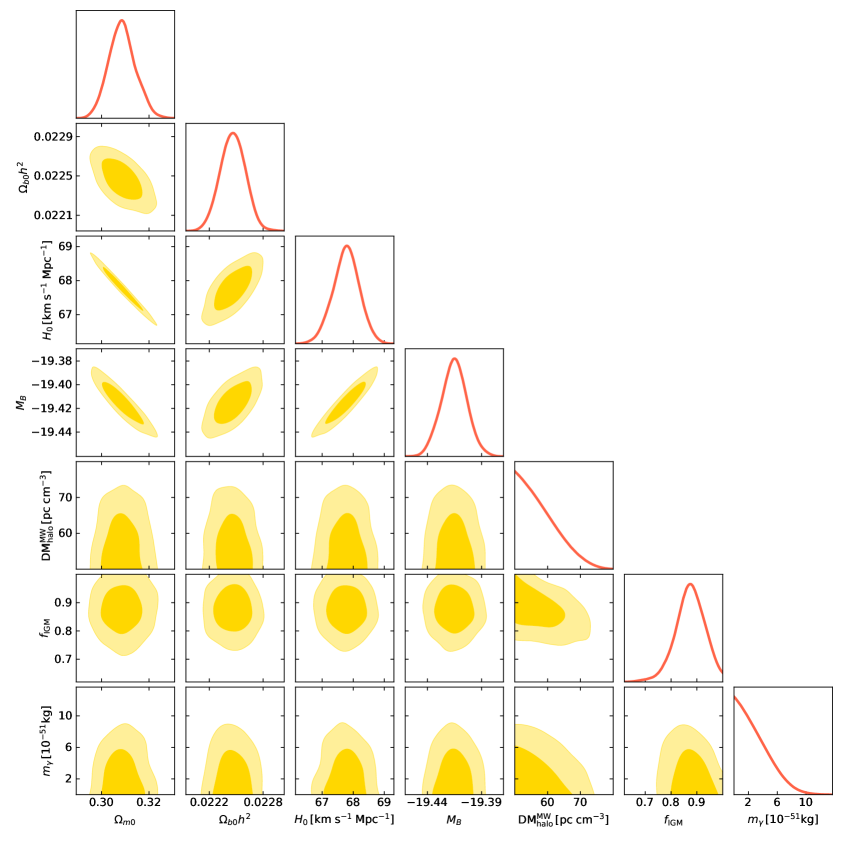
Figure 1: Posterior plots for the parameters $\Omega_{m0}$, $\Omega_{b0}h^{2}$, $H_{0}$, $M_{B}$, $\mathrm{DM_{halo}^{MW}}$, $f_{\rm IGM}$, and $m_{\gamma}$, constrained by the FRB, CMB, BAO, and SN Ia data. The contours show the 68% and 95% confidence intervals.

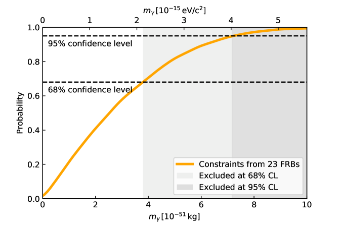
Figure 2: Cumulative posterior distribution for the photon mass $m_{\gamma}$. The grey areas mark the excluded values at $1\sigma$ and $2\sigma$ confidence levels.

Using the MCMC method, the marginalized $1\sigma$ constraints on these seven parameters are presented in Table 2. For the photon mass, both the $1\sigma$ and $2\sigma$ upper limits are displayed. The posterior distributions and the confidence contours for these parameters are plotted in Fig. 1. We find that the IGM baryon fraction is inferred to be $f_{\rm IGM}=0.873^{+0.061}_{-0.050}$, which is in good agreement with previous works [79, 56]. In Fig. 2, we show the cumulative posterior distribution of the photon mass $m_{\gamma}$. One can see from this plot that the $1\sigma$ and $2\sigma$ upper limits on $m_{\gamma}$ are

$$m_{\gamma}\leq 3.8\times 10^{-51}\,\rm{kg}\simeq 2.1\times 10^{-15}\,\rm{eV/c^{2}}$$ (3.2)

and

$$m_{\gamma}\leq 7.2\times 10^{-51}\,\rm{kg}\simeq 4.0\times 10^{-15}\,\rm{eV/c^{2}}\;,$$ (3.3)

respectively. Our results do not indicate that photons have definite mass, which means that the massless photon postulate is solid on the basis of the FRB measurements. We note that, compared with other cosmological probes, the FRB data have negligible effects on the estimated cosmological parameters. While the constraints on both $m_{\gamma}$ and $f_{\rm IGM}$ are drawn primarily from the FRB data.

Table 3 presents a summary of upper limits on the photon mass from FRBs. As an improvement over previous studies, the more realistic probability distributions of $\mathrm{DM_{IGM}}$ and $\mathrm{DM_{host}}$ with asymmetric tails to large-DM values have been considered in Wang et al. [29] (hereafter W21), Lin et al. [31] (hereafter L23), and our work. As shown in Table 3, W21 and L23 used a catalog of 129 FRBs and 17 localized FRBs to constrain the photon mass, yielding $m_{\gamma}\leq 3.1\times 10^{-51}\;\rm{kg}$ and $m_{\gamma}\leq 4.8\times 10^{-51}\;\rm{kg}$, respectively. These constraints are comparable to our result of $m_{\gamma}\leq 3.8\times 10^{-51}\;\rm{kg}$ at $1\sigma$ confidence level, however, it is still useful to compare differences in the analysis methods. Since most of the FRBs in their catalog have no redshift measurements, W21 had to use the observed $\mathrm{DM_{obs}}$ values to estimate the pseudo redshifts. Our photon mass limit from 23 localized FRBs is a little looser than that of W21, while avoiding potential bias from the estimation of redshift. Furthermore, neither W21 nor L23 accounted for the influence of the uncertainties of cosmological parameters on the photon mass limits. Unlike W21 and L23 that fix the cosmological parameters at certain values, we treat them as free parameters, so the effect caused by the uncertainties of cosmological parameters can be well handled in our analysis.

Table 3: A summary of upper limits on the photon rest mass $m_{\gamma}$ from FRBs.

Author (Year)	Sources	Frequency range	$m_{\gamma}$ ($\mathrm{kg}$)
Wu et al. (2016) [23]	FRB 150418	1.2–1.5 GHz	$5.2\times 10^{-50}$
Bonetti et al. (2016) [24]	FRB 150418	1.2–1.5 GHz	$3.2\times 10^{-50}$
Bonetti et al. (2017) [25]	FRB 121102	1.1–1.7 GHz	$3.9\times 10^{-50}$
Shao & Zhang (2017) [26]	21 FRBs (20 of them without	$\sim$GHz	$8.7\times 10^{-51}\;(1\sigma)$
	redshift measurement)		$1.5\times 10^{-50}\;(2\sigma)$
Xing et al. (2019) [27]	FRB 121102 subpulses	1.34–1.37 GHz	$5.1\times 10^{-51}$
Wei & Wu (2020) [28]	9 localized FRBs	$\sim$GHz	$7.1\times 10^{-51}\;(1\sigma)$
			$1.3\times 10^{-50}\;(2\sigma)$
Wang et al. (2021) [29]	129 FRBs (most of them without	$\sim$GHz	$3.1\times 10^{-51}\;(1\sigma)$
	redshift measurement)		$3.9\times 10^{-51}\;(2\sigma)$
Chang et al. (2023) [30]	FRB 180916Ba	124.8–185.7 MHz	$6.0\times 10^{-47}$
Lin et al. (2023) [31]	17 localized FRBs	$\sim$GHz	$4.8\times 10^{-51}\;(1\sigma)$
			$7.1\times 10^{-51}\;(2\sigma)$
This work	23 localized FRBs	$\sim$GHz	$3.8\times 10^{-51}\;(1\sigma)$
			$7.2\times 10^{-51}\;(2\sigma)$

Note.

^aThe limit of Ref. [30] was obtained based on the second-order photon mass effect.

4 Conclusions and Discussion

Cosmological FRBs have been proposed as an ideal probe for constraining the photon rest mass $m_{\gamma}$. Similar to the dispersion from the plasma, the time delay due to the $m_{\gamma}\neq 0$ effect is proportional to $\nu^{-2}$ in the first-order approximation. Therefore, a nonzero photon mass can produce an additional $\mathrm{DM}_{\gamma}$, which provides a theoretical basis to constrain $m_{\gamma}$. A key challenge in this dispersion method for constraining $m_{\gamma}$, however, is to distinguish $\mathrm{DM}_{\gamma}$ from other DMs contributed by the FRB host galaxy ($\mathrm{DM_{host}}$) and IGM ($\mathrm{DM_{IGM}}$). Moreover, another problem that hinders such studies is the strong degeneracy between $m_{\gamma}$ and cosmological parameters.

In this work, we revisited the photon mass from the most up-to-date sample of 23 localized FRBs. Unlike most of the previous works that assumed the $\mathrm{DM_{host}}$ value as an unknown constant and introduced a systematic uncertainty to account for the diversity of host galaxy contribution and the large IGM fluctuation, we considered the more realistic probability distributions of $\mathrm{DM_{IGM}}$ and $\mathrm{DM_{host}}$ derived from the IllustrisTNG simulation. Additionally, all previous studies fixed the cosmological parameters at certain values and neglected the parameter degeneracy. To account for the systematic uncertainty resulting from the choices of priors of cosmological parameters, it would be better to treat the cosmological parameters as free parameters and infer their values from the observational data. With this aim, we combined the DM–$z$ measurements from FRBs with the CMB, BAO, and SN Ia data to constrain cosmological parameters and $m_{\gamma}$ simultaneously.

In the light of the above method, we obtained a new upper limit on the photon mass at $1\sigma$ ($2\sigma$) confidence level, i.e., $m_{\gamma}\leq 3.8\times 10^{-51}\;\rm{kg}$, or equivalently $m_{\gamma}\leq 2.1\times 10^{-15}\,\rm{eV/c^{2}}$ ($m_{\gamma}\leq 7.2\times 10^{-51}\,\rm{kg}$, or equivalently $m_{\gamma}\leq 4.0\times 10^{-15}\,\rm{eV/c^{2}}$). Moreover, a reasonable estimation for the IGM baryon fraction is simultaneously achieved, i.e., $f_{\rm IGM}=0.873^{+0.061}_{-0.050}$, which is well consistent with other recent results [79, 56]. To illustrate the competitiveness of FRB constraints, in Fig. 3 we plot the constraints from all various (laboratory and astrophysical) methods. As shown in Fig. 3, by analyzing the mechanical stability of the magnetized gas in galaxies, Chibisov obtained the most stringent limit on the photon mass of $m_{\gamma}\leq 3\times 10^{-60}\,\rm{kg}$ [20]. However, Chibisov’s approach depends in a critical way on many assumptions, and the reliability of this result remains somewhat unclear. One can also see from Fig. 3 that the photon mass limit obtained from FRBs is ordinary, but it performs best within the same dispersion method.

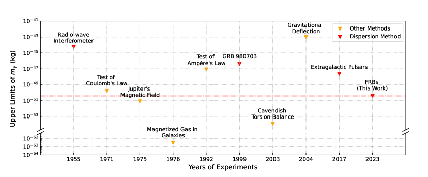
Figure 3: Upper limits on the photon mass from various experimental methods (in temporal order). The results obtained through the dispersion method are marked in red, including the limits from the radio-wave interferometer ($m_{\gamma}\leq 5.7\times 10^{-45}\;\rm{kg}$; [80]), GRB 980703 ($m_{\gamma}\leq 4.2\times 10^{-47}\;\rm{kg}$; [34]) , extragalactic pulsars ($m_{\gamma}\leq 2.3\times 10^{-48}\;\rm{kg}$; [36]), and FRBs ($m_{\gamma}\leq 3.8\times 10^{-51}\;\rm{kg}$; this work). The results obtained through other experimental methods are marked in orange, including test of Coulomb’s law ($m_{\gamma}\leq 1.6\times 10^{-50}\;\rm{kg}$; [15]), measurement of Jupiter’s magnetic field ($m_{\gamma}\leq 8\times 10^{-52}\;\rm{kg}$; [19]), test of Ampère’s law ($m_{\gamma}\leq 8.4\times 10^{-48}\;\rm{kg}$; [16]), the experiment of Cavendish torsion balance ($m_{\gamma}\leq 1.2\times 10^{-54}\;\rm{kg}$; [17]), analysis of the mechanical stability of the magnetized gas ($m_{\gamma}\leq 3\times 10^{-63}\;\rm{kg}$; [20]), and gravitational deflection of radio waves ($m_{\gamma}\leq 10^{-43}\;\rm{kg}$; [18]). The red dot-dashed line corresponds to the $1\sigma$ upper limit of $m_{\gamma}$ from FRBs.

In the end, we would like point out a caveat to our method. Throughout this article, we assume the standard $\Lambda$CDM cosmological model. But massive photons would change the cosmological model: for instance, producing non-cosmological redshifts, variations in the propagation of light, mass distribution during the history of the Universe, no need of dark energy, etc. In other words, our photon mass limits from cosmological FRBs are valid provided that the $\Lambda$CDM model is maintained even with a massive photon, which might be not the case if the mass of the photon is significantly different from zero.

References

- [1] L. De Broglie, Rayonnement noir et quanta de lumière, J. Phys. Radium 3 (1922) 422.
- [2] A. Proca, Sur la théorie ondulatoire des électrons positifs et négatifs, J. Phys. Radium 7 7 (1936) 347.
- [3] S. Kouwn, P. Oh and C.-G. Park, Massive photon and dark energy, Phys. Rev. D 93 (2016) 083012 [1512.00541].
- [4] D.F. Bartlett and J.P. Cumalat, How a Massive Photon Retards the Universal Expansion Until Galaxies Form, in AAS/Division of Dynamical Astronomy Meeting #42, vol. 42 of AAS/Division of Dynamical Astronomy Meeting, p. 4.03, Apr., 2011.
- [5] D.F. Roscoe, Maxwell’s Equations: New Light on Old Problems, Apeiron 13 (2006) 206.
- [6] J.P. Cumalat and D.F. Bartlett, Einstein, Schwinger, And The Sinusoidal Potential, in AAS/Division of Dynamical Astronomy Meeting, vol. 42 of AAS/Division of Dynamical Astronomy Meeting, p. 4.02, Apr., 2011.
- [7] A.D.A.M. Spallicci, J.A. Helayël-Neto, M. López-Corredoira and S. Capozziello, Cosmology and the massive photon frequency shift in the Standard-Model Extension, European Physical Journal C 81 (2021) 4 [2011.12608].
- [8] A.S. Goldhaber and M.M. Nieto, Terrestrial and Extraterrestrial Limits on The Photon Mass, Reviews of Modern Physics 43 (1971) 277.
- [9] D.D. Lowenthal, Limits on the Photon Mass, Phys. Rev. D 8 (1973) 2349.
- [10] Y.Z. Zhang, “Special Relativity And Its Experimental Foundation.” Special Relativity And Its Experimental Foundation. Series: Advanced Series on Theoretical Physical Science, ISBN: 978-981-02-2749-4. WORLD SCIENTIFIC, Edited by Yuan Zhong Zhang, vol. 4, Nov., 1997. 10.1142/3180.
- [11] L.-C. Tu, J. Luo and G.T. Gillies, The mass of the photon, Reports on Progress in Physics 68 (2005) 77.
- [12] L.B. Okun, Photon: History, Mass, Charge, Acta Physica Polonica B 37 (2006) 565 [hep-ph/0602036].
- [13] A.S. Goldhaber and M.M. Nieto, Photon and graviton mass limits, Reviews of Modern Physics 82 (2010) 939 [0809.1003].
- [14] G. Spavieri, J. Quintero, G.T. Gillies and M. Rodríguez, A survey of existing and proposed classical and quantum approaches to the photon mass, European Physical Journal D 61 (2011) 531.
- [15] E.R. Williams, J.E. Faller and H.A. Hill, New Experimental Test of Coulomb’s Law: A Laboratory Upper Limit on the Photon Rest Mass, Phys. Rev. Lett. 26 (1971) 721.
- [16] M.A. Chernikov, C.J. Gerber, H.R. Ott and H.J. Gerger, Erratum: Low-temperature upper limit of the photon mass: Experimental null test Ampères law, Phys. Rev. Lett. 69 (1992) 2999.
- [17] J. Luo, L.-C. Tu, Z.-K. Hu and E.-J. Luan, New Experimental Limit on the Photon Rest Mass with a Rotating Torsion Balance, Phys. Rev. Lett. 90 (2003) 081801.
- [18] A. Accioly and R. Paszko, Photon mass and gravitational deflection, Phys. Rev. D 69 (2004) 107501.
- [19] J. Davis, L., A.S. Goldhaber and M.M. Nieto, Limit on the Photon Mass Deduced from Pioneer-10 Observations of Jupiter’s Magnetic Field, Phys. Rev. Lett. 35 (1975) 1402.
- [20] G.V. Chibisov, FROM THE CURRENT LITERATURE: Astrophysical upper limits on the photon rest mass, Soviet Physics Uspekhi 19 (1976) 624.
- [21] R. Lakes, Experimental Limits on the Photon Mass and Cosmic Magnetic Vector Potential, Phys. Rev. Lett. 80 (1998) 1826.
- [22] M. López-Corredoira and J.I. Calvo-Torel, Fitting of supernovae without dark energy, International Journal of Modern Physics D 31 (2022) 2250104 [2207.14688].
- [23] X.-F. Wu, S.-B. Zhang, H. Gao, J.-J. Wei, Y.-C. Zou, W.-H. Lei et al., Constraints on the Photon Mass with Fast Radio Bursts, Astrophys. J. Lett. 822 (2016) L15 [1602.07835].
- [24] L. Bonetti, J. Ellis, N.E. Mavromatos, A.S. Sakharov, E.K. Sarkisyan-Grinbaum and A.D.A.M. Spallicci, Photon mass limits from fast radio bursts, Physics Letters B 757 (2016) 548 [1602.09135].
- [25] L. Bonetti, J. Ellis, N.E. Mavromatos, A.S. Sakharov, E.K. Sarkisyan-Grinbaum and A.D.A.M. Spallicci, FRB 121102 casts new light on the photon mass, Physics Letters B 768 (2017) 326 [1701.03097].
- [26] L. Shao and B. Zhang, Bayesian framework to constrain the photon mass with a catalog of fast radio bursts, Phys. Rev. D 95 (2017) 123010 [1705.01278].
- [27] N. Xing, H. Gao, J.-J. Wei, Z. Li, W. Wang, B. Zhang et al., Limits on the Weak Equivalence Principle and Photon Mass with FRB 121102 Subpulses, Astrophys. J. Lett. 882 (2019) L13 [1907.00583].
- [28] J.-J. Wei and X.-F. Wu, Combined limit on the photon mass with nine localized fast radio bursts, Research in Astronomy and Astrophysics 20 (2020) 206 [2006.09680].
- [29] H. Wang, X. Miao and L. Shao, Bounding the photon mass with cosmological propagation of fast radio bursts, Physics Letters B 820 (2021) 136596 [2103.15299].
- [30] C.-M. Chang, J.-J. Wei, S.-b. Zhang and X.-F. Wu, Bounding the photon mass with the dedispersed pulses of the Crab pulsar and FRB 180916B, J. Cosmol. Astropart. Phys. 2023 (2023) 010 [2207.00950].
- [31] H.-N. Lin, L. Tang and R. Zou, Revised constraints on the photon mass from well-localized fast radio bursts, Mon. Not. Roy. Astron. Soc. 520 (2023) 1324 [2301.12103].
- [32] B. Lovell, F.L. Whipple and L.H. Solomon, Relative Velocity of Light and Radio Waves in Space, Nature 202 (1964) 377.
- [33] B. Warner and R.E. Nather, Wavelength Independence of the Velocity of Light in Space, Nature 222 (1969) 157.
- [34] B.E. Schaefer, Severe Limits on Variations of the Speed of Light with Frequency, Phys. Rev. Lett. 82 (1999) 4964 [astro-ph/9810479].
- [35] B. Zhang, Y.-T. Chai, Y.-C. Zou and X.-F. Wu, Constraining the mass of the photon with gamma-ray bursts, Journal of High Energy Astrophysics 11 (2016) 20 [1607.03225].
- [36] J.-J. Wei, E.-K. Zhang, S.-B. Zhang and X.-F. Wu, New limits on the photon mass with radio pulsars in the Magellanic clouds, Research in Astronomy and Astrophysics 17 (2017) 13 [1608.07675].
- [37] J.-J. Wei and X.-F. Wu, Robust limits on photon mass from statistical samples of extragalactic radio pulsars, J. Cosmol. Astropart. Phys. 2018 (2018) 045 [1803.07298].
- [38] D.J. Bartlett, H. Desmond, P.G. Ferreira and J. Jasche, Constraints on quantum gravity and the photon mass from gamma ray bursts, Phys. Rev. D 104 (2021) 103516 [2109.07850].
- [39] J.-J. Wei and X.-F. Wu, Testing fundamental physics with astrophysical transients, Frontiers of Physics 16 (2021) 44300 [2102.03724].
- [40] M. McQuinn, Locating the “Missing” Baryons with Extragalactic Dispersion Measure Estimates, Astrophys. J. Lett. 780 (2014) L33 [1309.4451].
- [41] J.P. Macquart, J.X. Prochaska, M. McQuinn, K.W. Bannister, S. Bhandari, C.K. Day et al., A census of baryons in the Universe from localized fast radio bursts, Nature 581 (2020) 391 [2005.13161].
- [42] G.Q. Zhang, H. Yu, J.H. He and F.Y. Wang, Dispersion Measures of Fast Radio Burst Host Galaxies Derived from IllustrisTNG Simulation, Astrophys. J. 900 (2020) 170 [2007.13935].
- [43] Z.J. Zhang, K. Yan, C.M. Li, G.Q. Zhang and F.Y. Wang, Intergalactic Medium Dispersion Measures of Fast Radio Bursts Estimated from IllustrisTNG Simulation and Their Cosmological Applications, Astrophys. J. 906 (2021) 49 [2011.14494].
- [44] A. Walters, A. Weltman, B.M. Gaensler, Y.-Z. Ma and A. Witzemann, Future Cosmological Constraints From Fast Radio Bursts, Astrophys. J. 856 (2018) 65 [1711.11277].
- [45] L. Chen, Q.-G. Huang and K. Wang, Distance priors from Planck final release, J. Cosmol. Astropart. Phys. 2019 (2019) 028 [1808.05724].
- [46] Planck Collaboration, N. Aghanim, Y. Akrami, M. Ashdown, J. Aumont, C. Baccigalupi et al., Planck 2018 results. VI. Cosmological parameters, Astron. Astrophys. 641 (2020) A6 [1807.06209].
- [47] J. Ryan, Y. Chen and B. Ratra, Baryon acoustic oscillation, Hubble parameter, and angular size measurement constraints on the Hubble constant, dark energy dynamics, and spatial curvature, Mon. Not. Roy. Astron. Soc. 488 (2019) 3844 [1902.03196].
- [48] D.M. Scolnic, D.O. Jones, A. Rest, Y.C. Pan, R. Chornock, R.J. Foley et al., The Complete Light-curve Sample of Spectroscopically Confirmed SNe Ia from Pan-STARRS1 and Cosmological Constraints from the Combined Pantheon Sample, Astrophys. J. 859 (2018) 101 [1710.00845].
- [49] M.J. Bentum, L. Bonetti and A.D.A.M. Spallicci, Dispersion by pulsars, magnetars, fast radio bursts and massive electromagnetism at very low radio frequencies, Advances in Space Research 59 (2017) 736 [1607.08820].
- [50] W. Deng and B. Zhang, Cosmological Implications of Fast Radio Burst/Gamma-Ray Burst Associations, Astrophys. J. Lett. 783 (2014) L35 [1401.0059].
- [51] K. Ioka, The Cosmic Dispersion Measure from Gamma-Ray Burst Afterglows: Probing the Reionization History and the Burst Environment, Astrophys. J. Lett. 598 (2003) L79 [astro-ph/0309200].
- [52] S. Inoue, Probing the cosmic reionization history and local environment of gamma-ray bursts through radio dispersion, Mon. Not. Roy. Astron. Soc. 348 (2004) 999 [astro-ph/0309364].
- [53] A.A. Meiksin, The physics of the intergalactic medium, Reviews of Modern Physics 81 (2009) 1405 [0711.3358].
- [54] J.M. Shull, B.D. Smith and C.W. Danforth, The Baryon Census in a Multiphase Intergalactic Medium: 30% of the Baryons May Still be Missing, Astrophys. J. 759 (2012) 23 [1112.2706].
- [55] A. Walters, Y.-Z. Ma, J. Sievers and A. Weltman, Probing diffuse gas with fast radio bursts, Phys. Rev. D 100 (2019) 103519 [1909.02821].
- [56] B. Wang and J.-J. Wei, An 8.0% Determination of the Baryon Fraction in the Intergalactic Medium from Localized Fast Radio Bursts, Astrophys. J. 944 (2023) 50 [2211.02209].
- [57] J.M. Cordes and T.J.W. Lazio, NE2001.I. A New Model for the Galactic Distribution of Free Electrons and its Fluctuations, arXiv e-prints (2002) astro [astro-ph/0207156].
- [58] J.X. Prochaska and Y. Zheng, Probing Galactic haloes with fast radio bursts, Mon. Not. Roy. Astron. Soc. 485 (2019) 648 [1901.11051].
- [59] Q. Wu, G.-Q. Zhang and F.-Y. Wang, An 8 per cent determination of the Hubble constant from localized fast radio bursts, Mon. Not. Roy. Astron. Soc. 515 (2022) L1 [2108.00581].
- [60] V. Springel, R. Pakmor, A. Pillepich, R. Weinberger, D. Nelson, L. Hernquist et al., First results from the IllustrisTNG simulations: matter and galaxy clustering, Mon. Not. Roy. Astron. Soc. 475 (2018) 676 [1707.03397].
- [61] S. Chatterjee, C.J. Law, R.S. Wharton, S. Burke-Spolaor, J.W.T. Hessels, G.C. Bower et al., A direct localization of a fast radio burst and its host, Nature 541 (2017) 58 [1701.01098].
- [62] S. Bhandari, K.E. Heintz, K. Aggarwal, L. Marnoch, C.K. Day, J. Sydnor et al., Characterizing the Fast Radio Burst Host Galaxy Population and its Connection to Transients in the Local and Extragalactic Universe, Astron. J. 163 (2022) 69 [2108.01282].
- [63] B. Marcote, K. Nimmo, J.W.T. Hessels, S.P. Tendulkar, C.G. Bassa, Z. Paragi et al., A repeating fast radio burst source localized to a nearby spiral galaxy, Nature 577 (2020) 190 [2001.02222].
- [64] K.W. Bannister, A.T. Deller, C. Phillips, J.P. Macquart, J.X. Prochaska, N. Tejos et al., A single fast radio burst localized to a massive galaxy at cosmological distance, Science 365 (2019) 565 [1906.11476].
- [65] J.X. Prochaska, J.-P. Macquart, M. McQuinn, S. Simha, R.M. Shannon, C.K. Day et al., The low density and magnetization of a massive galaxy halo exposed by a fast radio burst, Science 366 (2019) 231 [1909.11681].
- [66] S. Bhandari, E.M. Sadler, J.X. Prochaska, S. Simha, S.D. Ryder, L. Marnoch et al., The Host Galaxies and Progenitors of Fast Radio Bursts Localized with the Australian Square Kilometre Array Pathfinder, Astrophys. J. Lett. 895 (2020) L37 [2005.13160].
- [67] V. Ravi, M. Catha, L. D’Addario, S.G. Djorgovski, G. Hallinan, R. Hobbs et al., A fast radio burst localized to a massive galaxy, Nature 572 (2019) 352 [1907.01542].
- [68] J.S. Chittidi, S. Simha, A. Mannings, J.X. Prochaska, S.D. Ryder, M. Rafelski et al., Dissecting the Local Environment of FRB 190608 in the Spiral Arm of its Host Galaxy, Astrophys. J. 922 (2021) 173 [2005.13158].
- [69] K.E. Heintz, J.X. Prochaska, S. Simha, E. Platts, W.-f. Fong, N. Tejos et al., Host Galaxy Properties and Offset Distributions of Fast Radio Bursts: Implications for Their Progenitors, Astrophys. J. 903 (2020) 152 [2009.10747].
- [70] C.J. Law, B.J. Butler, J.X. Prochaska, B. Zackay, S. Burke-Spolaor, A. Mannings et al., A Distant Fast Radio Burst Associated with Its Host Galaxy by the Very Large Array, Astrophys. J. 899 (2020) 161 [2007.02155].
- [71] V. Ravi, C.J. Law, D. Li, K. Aggarwal, M. Bhardwaj, S. Burke-Spolaor et al., The host galaxy and persistent radio counterpart of FRB 20201124A, Mon. Not. Roy. Astron. Soc. 513 (2022) 982 [2106.09710].
- [72] C.W. James, E.M. Ghosh, J.X. Prochaska, K.W. Bannister, S. Bhandari, C.K. Day et al., A measurement of Hubble’s Constant using Fast Radio Bursts, Mon. Not. Roy. Astron. Soc. 516 (2022) 4862 [2208.00819].
- [73] S.D. Ryder, K.W. Bannister, S. Bhandari, A.T. Deller, R.D. Ekers, M. Glowacki et al., Probing the distant universe with a very luminous fast radio burst at redshift 1, arXiv e-prints (2022) arXiv:2210.04680 [2210.04680].
- [74] M. Bhardwaj, B.M. Gaensler, V.M. Kaspi, T.L. Landecker, R. Mckinven, D. Michilli et al., A Nearby Repeating Fast Radio Burst in the Direction of M81, Astrophys. J. Lett. 910 (2021) L18 [2103.01295].
- [75] F. Kirsten, B. Marcote, K. Nimmo, J.W.T. Hessels, M. Bhardwaj, S.P. Tendulkar et al., A repeating fast radio burst source in a globular cluster, Nature 602 (2022) 585 [2105.11445].
- [76] M. Bhardwaj, A.Y. Kirichenko, D. Michilli, Y.D. Mayya, V.M. Kaspi, B.M. Gaensler et al., A Local Universe Host for the Repeating Fast Radio Burst FRB 20181030A, Astrophys. J. Lett. 919 (2021) L24 [2108.12122].
- [77] C.H. Niu, K. Aggarwal, D. Li, X. Zhang, S. Chatterjee, C.W. Tsai et al., A repeating fast radio burst associated with a persistent radio source, Nature 606 (2022) 873 [2110.07418].
- [78] D. Foreman-Mackey, D.W. Hogg, D. Lang and J. Goodman, emcee: The MCMC Hammer, Publications of the Astronomical Society of the Pacific 125 (2013) 306 [1202.3665].
- [79] Z. Li, H. Gao, J.J. Wei, Y.P. Yang, B. Zhang and Z.H. Zhu, Cosmology-insensitive estimate of IGM baryon mass fraction from five localized fast radio bursts, Mon. Not. Roy. Astron. Soc. 496 (2020) L28 [2004.08393].
- [80] E.F. Florman, A measurement of the velocity of propagation of very-high-frequency radio waves at the surface of the earth, Journal of Research of the National Bureau of Standards 54 (1955) .