1D approximation of measures in Wasserstein spaces

Abstract.

We propose a variational approach to approximate measures with measures uniformly distributed over a 1 dimentional set. The problem consists in minimizing a Wasserstein distance as a data term with a regularization given by the length of the support. As it is challenging to prove existence of solutions to this problem, we propose a relaxed formulation, which always admits a solution. In the sequel we show that if the ambient space is $\mathbb{R}^{2}$, under techinical assumptions, any solution to the relaxed problem is a solution to the orginal one. Finally we manage to prove that any optimal solution to the relaxed problem, and hence also to the original, is Ahlfors regular.

1. Introduction

In this paper we study the following 1D-shape optimization problem: given a reference probability measure $\rho_{0}\in\mathcal{P}_{p}(\mathbb{R}^{d})$ (the set of probability measures $\rho$ with $\int_{\mathbb{R}^{d}}|x|^{p}d\rho<+\infty$, $p\geq 1$), we seek to approximate $\rho_{0}$ with measures supported over a connected subset of $\mathbb{R}^{d}$. This approximation is done by means of the following variational problem

($$P_{\Lambda} \mathop{\rm inf}_{\Sigma\in\mathcal{A}}W_{p}^{p}(\rho_{0},\nu_{\Sigma})+\Lambda\mathcal{H}^{1}(\Sigma),$$)

where the measure $\nu_{\Sigma}$ is defined as

(1.1) $$\nu_{\Sigma}:=\frac{1}{\mathcal{H}^{1}(\Sigma)}\mathcal{H}^{1}\mathbin{\vrule height=6.88889pt,depth=0.0pt,width=0.55974pt\vrule height=0.55974pt,depth=0.0pt,width=5.59721pt}\Sigma,\text{ for }\Sigma\in\mathcal{A}:=\left\{\Sigma\subset\mathbb{R}^{d}:\begin{array}[]{c}0<\mathcal{H}^{1}(\Sigma)<+\infty\\ \text{ compact, connected.}\end{array}\right\},$$

and $\mathcal{H}^{1}$ denotes the 1-dimensional Hausdorff measure in $\mathbb{R}^{d}$. The term $W_{p}$ denotes the usual Wasserstein distance on the space of probability measures (see [29, 31] and Section 2.1.2).

One can trace the idea of approximating a probability measure by a 1D set back to the concept of principal curves from the seminal paper [16], which extends linear regression to regression using general curves, and introduces a variational problem to define such curves. In this variational sense, a principal curve minimizes the expectation of the distance to the curve, w.r.t. a probability measure describing a data set (with some regularization to ensure existence). As proposed in [17], a length constraint is a simple and intrinsic way too ensure existence. The properties of such minimizers have been studied in detail in e.g. [20, 11].

A further generalization consists in replacing the curve with a more general one-dimensional compact and connected set, yielding the average distance minimizer problem introduced in [7], and its dual counterpart maximum distance minimizer problem [25, 19]. Such problems were conceived for applications in urban planning, where one seeks to minimize the average distance to a transportation network, giving rise to the need for a larger class of 1D sets allowing for bifurcations.

While the above-mentioned problems only focus on some geometric approximation of the support of the measure, approximating a measure in the sense of weak convergence is sometimes more desirable. In [18, 8], the authors have proposed optimal transport based methods for the projection of probability measures onto classes of measures supported on simple curves, using the Wasserstein distance as a data term. Potential applications range from 3D printing to image compression and reconstruction. In [12], the data fidelity term is chosen to be a discrepancy, see also [24]. The advantage of using discrepancies is that approximation rates can be given independently from the dimension, being therefore a good alternative to overcome the curse of dimensionality. The problem we study is an attempt to generalize this class of problems to the approximation with one-dimensional connected sets.

One difficulty when studying ($P_{\Lambda}$) is that the class of measures $\nu_{\Sigma}$ is not closed in the usual weak topologies considered for the space of probability measures. While a sequence of sets $(\Sigma_{n})_{n\in\mathbb{N}}$ in $\mathcal{A}$ with uniformly bounded length will have subsequences converging (in the Hausdorff sense) either to a point or a set in $\mathcal{A}$, the corresponding measures $\nu_{\Sigma_{n}}$ might converge to a measure which is not necessarily uniform on that set: longer parts of $\Sigma_{n}$ might concentrate in the limit on shorter parts of $\Sigma$. Hence minimzing sequences might in general converge to measures which are not of the form $\nu_{\Sigma}$, and we need to determine a proper relaxation of our energy. The relaxed energy has the form

($$\overline{P}_{\Lambda} \mathop{\rm inf}_{\begin{subarray}{c}\nu\in\mathcal{P}_{p}(\mathbb{R}^{d})\end{subarray}}W_{p}^{p}(\rho_{0},\nu)+\Lambda\mathcal{L}(\nu)$$)

where $\mathcal{L}$, the length functional, defined in Section 3.1, generalizes the notion of length of the support of a measure, having the property that $\mathcal{L}(\nu)<\infty$ if and only if $\mathop{\rm supp}\nu\in\mathcal{A}$ or $\nu$ is a Dirac mass. The following theorem gathers the various results proved throughout this paper.

Theorem 1.1.

Let $\rho_{0}\in\mathcal{P}_{p}(\mathbb{R}^{d})$, $\Lambda>0$. Then ($\overline{P}_{\Lambda}$) admits a solution $\nu$, and there exists $\Lambda_{\star}\geq 0$ such that if $\Lambda>\Lambda_{\star}$, $\nu$ is a Dirac mass. For $\Lambda<\Lambda_{\star}$, $\nu$ is supported by a set $\Sigma\in\mathcal{A}$ and the following properties hold.

1. If $\rho_{0}$ is absolutely continuous w.r.t. $\mathcal{H}^{1}$, or has a $L^{\infty}$ density w.r.t. $\mathcal{H}^{1}$), then so does $\nu$.

2. For $d=2$, if $\rho_{0}$ does not give mass to $1D$ sets, then $\nu=\nu_{\Sigma}$ and therefore is a solution to the original problem ($P_{\Lambda}$).

3. If $\rho_{0}\in L^{\frac{d}{d-1}}(\mathbb{R}^{d})$, then $\Sigma$ is Ahlfors regular, i.e. there is $r_{0}$ depending on $d,p,\rho_{0}$ and $\mathcal{L}(\nu)$ and $C$ depending only on $d,p$ such that for any $x\in\Sigma$ and $r\leq r_{0}$ it holds that

   $$r\leq\mathcal{H}^{1}(\Sigma\cap B_{r}(x))\leq Cr.$$

The paper is organized as follows: in Section 2 we recall a few tools from optimal transport and geometric measure theory. Next, in section 3 we go through the definition of the length functional and its properties as well as the relaxed problem and existence of solution for it. In section 4 we discuss the existence of $\Lambda_{*}$. In Section 5 (Theorem 5.4) we prove point (1) from Theorem 1.1, while the existence in 2D is proved in Section 6 (Theorem 6.3), and the Ahlfors regularity is studied in Section 7.

2. Preliminaries

We start by introducing notions of convergence for sets and measures which will be useful to study problem ($P_{\Lambda}$) as well as the relaxed one ($\overline{P}_{\Lambda}$). Next we describe some intrumental properties of the objects we shall use throughout the paper, namely the rectifiable sets and measures.

2.1. Convergence of sets and measures

2.1.1. Hausdorff and Kuratowski convergence

We recall some useful definitions of convergence for sets, see for instance [27, Chap. 4], [3, Chap. 6].

A sequence of closed subsets of $\mathbb{R}^{d}$ $\left(A_{n}\right)_{n\in\mathbb{N}}$ converges in the Hausdorff sense to $A$ if $d_{H}(A_{n},A)\xrightarrow[n\to\infty]{}0$, where $d_{H}$ is called the Hausdorff distance and is defined as

(2.1) $$d_{H}(A,B):=\mathop{\rm max}\left\{\sup_{a\in A}\mathop{\rm dist}(a,B),\sup_{b\in B}\mathop{\rm dist}(b,A)\right\},\text{ we write $A_{n}\xrightarrow[n\to\infty]{d_{H}}A$,}$$

where $\mathop{\rm dist}(\cdot,A)$ denotes the distance function to the set $A$. One can prove that this notion of convergence is equivalent to uniform convergence of the distance functions. Since the latter are all 1-Lipschitz, as a consequence of Arzela-Ascoli’s Theorem it follows that if the sequence is contained in a compact set, one can always extract a convergent subsequence. This compactness result is known as Blaschke’s Theorem, see [3, Theorem 6.1].

A sequence of closed sets $C_{n}$ converges in the sense of Kuratowski to $C$, and we write $C_{n}\xrightarrow[n\to\infty]{K}C$, whenever the two properties hold:

1. Given a sequence $x_{n}\in C_{n}$, all its cluster points are contained in $C$.

2. For all points $x\in C$ there exists a sequence $x_{n}\in C_{n}$, converging to $x$.

Again, one can show that $C_{n}\to C$ in the sense of Kuratowski if and only if $\mathop{\rm dist}(x,C_{n})\to\mathop{\rm dist}(x,C)$ (possibly infinite if $C=\emptyset$) locally uniformly (see [27, Cor. 4.7]). In addition, Kuratowski convergence also induces a compact topology, i.e. any sequence of closed sets has a subsequence which converges, possibly to the empty set.

The following Lemma describes a relation between Hausdorff and Kuratowski convergences. We prove it in Appendix B.

Lemma 2.1.

Let $(C_{n})_{n\in\mathbb{N}}$ be a sequence of closed sets in $\mathbb{R}^{d}$, converging to $C$ in the sense of Kuratowski. Then, for any $x\in\mathbb{R}^{d}$,

$$C_{n}\cap\overline{B_{R}(x)}\xrightarrow[n\to\infty]{d_{H}}C\cap\overline{B_{R}(x)},$$

for every radius $R>0$ such that $\overline{C\cap B_{R}(x)}=C\cap\overline{B}_{R}(x)$. Moreover, that condition holds for all $R>0$ except in a countable set.

2.1.2. Optimal transport and the Wasserstein distance

The Wasserstein distances $W_{p}$ are defined through the value function of an optimal transport problem, see [1, 29, 31] for details. Given two probability measures $\mu,\nu\in\mathcal{P}_{p}(\mathbb{R}^{d})$, we set

(2.2) $$W_{p}^{p}(\mu,\nu)\stackrel{{\scriptstyle\mbox{\tiny def.}}}{{=}}\mathop{\rm min}_{\gamma\in\Pi(\mu,\nu)}\int_{\mathbb{R}^{d}\times\mathbb{R}^{d}}|x-y|^{p}{\rm d}\gamma,$$

where $\displaystyle\Pi(\mu,\nu):=\left\{\gamma\in\mathcal{P}\left(\mathbb{R}^{d}\times\mathbb{R}^{d}\right):\quad{\pi_{0}}_{\sharp}\gamma=\mu,\ {\pi_{1}}_{\sharp}\gamma=\nu\right\}$ is the space of transport couplings, and $\pi_{i}$ denote the projections, i.e. $\pi_{0}(x,y)=x$ and $\pi_{1}(x,y)=y$. Whenever $\mu$ does not have atoms, the value of (2.2) coincides with

(2.3) $$\mathop{\rm inf}_{\begin{subarray}{c}T_{\sharp}\mu=\nu\end{subarray}}\int_{\mathbb{R}^{d}}|x-T(x)|^{p}{\rm d}\mu,$$

where the inf is taken over all measurable maps $T$ such that $T_{\sharp}\mu(A)=\nu(A)=\mu(T^{-1}(A))$ for any Borel set $A$.

The optimal transport problem can be analogously defined for any pair of positive $\mu,\nu$ on the space $\mathcal{M}(\mathbb{R}^{d})$ of Radon measures. In this case the Wasserstein distance becomes a 1-homogeneous functional and is finite if and only if the measures have finite $p$-moments and the same total mass $\mu(\mathbb{R}^{d})=\nu(\mathbb{R}^{d})$.

Definition 2.1.

Given a sequence $\left(\mu_{n}\right)_{n\in\mathbb{N}}\subset\mathcal{P}(\mathbb{R}^{d})$, we say it converges in a weak sense to $\mu$, if for a suitable space of functions $X$ we have

$$\int_{\mathbb{R}^{d}}\phi{\rm d}\mu_{n}\xrightarrow[n\to\infty]{}\int_{\mathbb{R}^{d}}\phi{\rm d}\mu\text{ for all $\phi\in X$.}$$

When $X=C_{b}(\mathbb{R}^{d})$, the space of bounded continuous functions, we say that $\mu_{n}$ converges narrowly to $\mu$ and we write $\mu\xrightharpoonup[n\to\infty]{}\mu$.

When $X=C_{0}(\mathbb{R}^{d})$, the space of continuous functions converging to $0$ at infinity, we say that $\mu_{n}$ converges to $\mu$ in the weak-$\star$ sense and we write $\mu\xrightharpoonup[n\to\infty]{\star}\mu$.

The Wasserstein distance is l.s.c. with respect to the narrow convergence, and continuous in a compact domain, [31, Lemma 4.3], on the other hand probability measures are compact for the weak-$\star$ convergence (but the limit might not be a probability measure) [28, 13]. Compactness for the narrow convergence needs the assumptions of Prokhorov’s Theorem, see [2, Theorem 2.8].

For a general (open) domain $\Omega$ we have $C_{c}(\Omega)\subset C_{0}(\Omega)\subset C_{b}(\Omega)$ with strict inclusion. If on the other hand $\Omega$ is a compact domain all these spaces coincide and so the notions of narrow and weak-$\star$ convergence are equivalent.

2.2. Golab’s Theorem

We now study the lower semicontinuity of ($P_{\Lambda}$). First, “Gołab’s Theorem” [15] shows that along sequences of connected sets, $\mathcal{H}^{1}$ is l.s.c. with respect to the Hausdorff convergence [22, Chapter 10]. It is of course also true if the sequence has a uniformly bounded number of connected components.

The issue is that the compactness of Hausdorff convergence is not transfered to the weak convergence of measures of the form $\mathcal{H}^{1}\mathbin{\vrule height=6.88889pt,depth=0.0pt,width=0.55974pt\vrule height=0.55974pt,depth=0.0pt,width=5.59721pt}\Sigma$ which may concentrate in the limit. In general, one can prove the following:

Theorem 2.2 (Density version of Golab’s Theorem).

Let ${(\Sigma_{n})}_{n\in\mathbb{N}}$ be a sequence of closed and connected subsets of $\mathbb{R}^{d}$ converging in the sense of Kuratowski to some closed set $\Sigma$ and having locally uniform finite length, i.e. for all $R>0$

$$\sup_{n\in\mathbb{N}}\mathcal{H}^{1}(\Sigma_{n}\cap B_{R}(x_{0}))<+\infty.$$

Define the measures $\mu_{n}:=\mathcal{H}^{1}\mathbin{\vrule height=6.88889pt,depth=0.0pt,width=0.55974pt\vrule height=0.55974pt,depth=0.0pt,width=5.59721pt}\Sigma_{n}$, and let $\mu$ be a weak-$\star$ cluster point of this sequence. Then $\mathop{\rm supp}\mu\subset\Sigma$ and it holds that

$$\mu\geq\mathcal{H}^{1}\mathbin{\vrule height=6.88889pt,depth=0.0pt,width=0.55974pt\vrule height=0.55974pt,depth=0.0pt,width=5.59721pt}\Sigma,$$

in the sense of measures.

This result is hidden in the proof in [4] of the usual thesis of Golab’s Theorem, see also [26]. For the reader’s convenience we give a simple proof in Appendix B.

Remark 2.3.

As we have not used any properties from the vector space structure of $\mathbb{R}^{d}$, this proof works in the case a locally compact metric space, as in [4].

2.3. Rectifiable sets and measures

We now introduce the notions of rectifiable sets and rectifiable measure, which will be crucial for understanding the fine properties of the elements of $\mathcal{A}$.

Definition 2.2.

Let $M\subset\mathbb{R}^{d}$ be a Borel set and $k\in\mathbb{N}$, we say that $M$ is countably $\mathcal{H}^{k}$-rectifiable, or shortly $k$ rectifiable, if there are countably many Lipschitz functions $f_{i}:\mathbb{R}^{k}\to\mathbb{R}^{d}$ such that

$$\mathcal{H}^{k}\left(M\setminus\bigcup_{i\in\mathbb{N}}f_{i}\left(\mathbb{R}^{k}\right)\right)=0.$$

A Radon measure $\mu$ is said to be $k$-rectifiable if it is supported over a $k$-rectifiable set and $\mu\ll\mathcal{H}^{k}$.

In the simple case $M=f(E)$, for $E\subset\mathbb{R}^{k}$, one can define the tangent space at a point of differentiability of $f$ as

$$\nabla f(z)\left(\mathbb{R}^{k}\right),\text{ for $x=f(z)$}.$$

This is a parametric definition that can be extended to $k$-rectifiable sets. It turns out the parametric notion of tangentiability can be expressed in terms of measure theory. Given a Borel set $M$, we set the measure $\mu=\mathcal{H}^{k}\mathbin{\vrule height=6.88889pt,depth=0.0pt,width=0.55974pt\vrule height=0.55974pt,depth=0.0pt,width=5.59721pt}M$, and we consider the family of blow-up measures

(2.4) $$\mu_{r}:=r^{-k}\Phi^{x,r}_{\sharp}\mu=\mathcal{H}^{k}\mathbin{\vrule height=6.88889pt,depth=0.0pt,width=0.55974pt\vrule height=0.55974pt,depth=0.0pt,width=5.59721pt}\left(\frac{M-x}{r}\right),\text{ for }\Phi^{x,r}:=\frac{\text{id}-x}{r}.$$

The blow-up Theorem, see [21, Theorem 10.2], states that for $\mathcal{H}^{k}$-a.e. $x\in M$ this family of measures converges in the weak-$\star$ topology to a measure of the form $\mathcal{H}^{k}\mathbin{\vrule height=6.88889pt,depth=0.0pt,width=0.55974pt\vrule height=0.55974pt,depth=0.0pt,width=5.59721pt}\pi_{x}$, for a unique $k$-plane $\pi_{x}\in\text{G}(k,d)$, the Grassmannian of $k$-planes of $\mathbb{R}^{d}$.

More generally define the $k$-density, whenever the limit exists, of a Radon measure $\mu$ as

(2.5) $$\theta_{k}(\mu,x)\stackrel{{\scriptstyle\mbox{\tiny def.}}}{{=}}\lim_{r\to 0^{+}}\frac{\mu(B_{r}(x))}{\omega_{k}r^{k}}\text{ and }\theta_{k}(M,x)\stackrel{{\scriptstyle\mbox{\tiny def.}}}{{=}}\theta_{k}\left(\mathcal{H}^{k}\mathbin{\vrule height=6.88889pt,depth=0.0pt,width=0.55974pt\vrule height=0.55974pt,depth=0.0pt,width=5.59721pt}M,x\right),$$

where $\omega_{k}$ is the volume of the unit $k$-dimensional ball, see [3, 21]. A direct consequence of the blow-up Theorem is that $\mathcal{H}^{k}$-a.e. point of a $k$-rectifiable set has $k$-density $1$. Analogously for a $k$-rectifiable measure $\mu$ it holds that $\mu=\theta_{k}(\mu,x)\mathcal{H}^{k}\mathbin{\vrule height=6.88889pt,depth=0.0pt,width=0.55974pt\vrule height=0.55974pt,depth=0.0pt,width=5.59721pt}M$.

The equivalence between all notions was completed with the work of Preiss and the notion of a tangent space to a measure, see for instance the monograph [10]. If a measures (resp. a set) has a finite $k$-density, i.e. the limit in (2.5) exists and is finite $\mathcal{H}^{k}$-a.e., then this measure (resp. set) is $k$-rectifiable. The previous discussion is summarized in the following theorem.

Theorem 2.4.

Let $\mu$ be a Radon measure over $\mathbb{R}^{d}$, the following are equivalent.

1. $\mu$ is $k$-rectifiable

2. For $\mathcal{H}^{k}$-a.e. $x\in\mathop{\rm supp}\mu$, it holds that

   $$r^{-k}\Phi^{x,r}_{\sharp}\mu\xrightharpoonup[r\to 0]{\star}\theta_{k}(\mu,x)\mathcal{H}^{k}\mathbin{\vrule height=6.88889pt,depth=0.0pt,width=0.55974pt\vrule height=0.55974pt,depth=0.0pt,width=5.59721pt}\pi_{x},$$

   for a unique $k$-plane $\pi_{x}\in\text{G}(k,d)$.

3. For $\mathcal{H}^{k}$-a.e. $x\in\mathop{\rm supp}\mu$, the $k$-density of $\mu$ in (2.5) exists and is finite.

In the previous Theorem, if we take $\mu=\mathcal{H}^{k}\mathbin{\vrule height=6.88889pt,depth=0.0pt,width=0.55974pt\vrule height=0.55974pt,depth=0.0pt,width=5.59721pt}M$ where $M$ is a countably $\mathcal{H}^{k}$-rectifiable set we define the approximate tangent space of $M$ at $x$ as $T_{x}M\stackrel{{\scriptstyle\mbox{\tiny def.}}}{{=}}\pi_{x}$, where $\pi_{x}$ is the unique $k$-plane from point (ii).

Definition 2.3.

Let $M\subset\mathbb{R}^{d}$ be a $k$-rectifiable set. We say that $x\in M$ is a rectifiability point when the weak-$\star$ convergence of point (ii) from Theorem 2.4 holds, with $\mu=\mathcal{H}^{k}\mathbin{\vrule height=6.88889pt,depth=0.0pt,width=0.55974pt\vrule height=0.55974pt,depth=0.0pt,width=5.59721pt}M$.

Now we pass to our case of interest, the 1-dimensional sets $\Sigma\in\mathcal{A}$, recall the definition (1.1). These sets are known to be $1$-rectifiable, see [4, Thm. 4.4.8], and hence they enjoy the properties of Theorem 2.4. In the next Lemma, we show that the blow-up of some $\Sigma\in\mathcal{A}$ around a rectifiability point is precisely its approximate tangent space.

Lemma 2.5.

Given $\Sigma\in\mathcal{A}$, then for $\mathcal{H}^{1}$-a.e. $y\in\Sigma$, it holds that

$$\frac{\Sigma-y}{r}\xrightarrow[r\to 0^{+}]{K}T_{y}\Sigma\quad\text{and}\quad\frac{\Sigma-y}{r}\cap B_{R}(0)\xrightarrow[r\to 0^{+}]{d_{H}}T_{y}\Sigma\cap B_{R}(0),\text{ for all $R>0$.}$$

Proof.

First we take a rectifiability point $y\in\Sigma$ with tangent space $T_{y}\Sigma$, by Theorem 2.4 such points cover $\mathcal{H}^{1}$ a.a. of $\Sigma$. In particular, point (ii) of the theorem shows that $\mathcal{H}^{1}\mathbin{\vrule height=6.88889pt,depth=0.0pt,width=0.55974pt\vrule height=0.55974pt,depth=0.0pt,width=5.59721pt}((\Sigma-y)/r)\xrightharpoonup[r\to 0]{\star}\mathcal{H}^{1}\mathbin{\vrule height=6.88889pt,depth=0.0pt,width=0.55974pt\vrule height=0.55974pt,depth=0.0pt,width=5.59721pt}T_{y}\Sigma$. Let $T$ be the (Kuratowski) limit of a subsequence $(\Sigma-y)/r_{k}$. Clearly, the limit measure $\mathcal{H}^{1}\mathbin{\vrule height=6.88889pt,depth=0.0pt,width=0.55974pt\vrule height=0.55974pt,depth=0.0pt,width=5.59721pt}T_{y}\Sigma$ is supported by $T$, hence $T_{y}\Sigma\subset T$. Thanks to Lemma 2.1 and Theorem 2.2, for almost all $R>0$,

(2.6) $$\mathcal{H}^{1}(T\cap B_{R})\leq\liminf_{k\to\infty}\mathcal{H}^{1}\left(\frac{\Sigma-y}{r_{k}}\cap B_{R}\right)=\mathcal{H}^{1}(T_{y}\Sigma\cap B_{R}),$$

which shows that up to a $\mathcal{H}^{1}$-negligible set, $T=T_{y}\Sigma$.

Notice that, if there is some $x\in T\setminus T_{y}\Sigma$, we may consider some ball $B_{s}(x)$ which does not intersect $T_{y}\Sigma$. Since $T$ is the limit of connected sets, $x$ must be path-connected in $T$ to some point in $(B_{s}(x))^{c}$, so that $\mathcal{H}^{1}(T\cap B_{s}(x))\geq s$. This contradicts (2.6). Hence $T=T_{y}\Sigma$, and is independent on the subsequence, and we deduce that $(\Sigma-y)/r\stackrel{{\scriptstyle K}}{{\to}}T_{y}\Sigma$. ∎

3. The length functional and the relaxed problem

If a minimizing sequence $\Sigma_{n}$ converges to some set $\Sigma$, we cannot expect the weak limit of (some subsequence of) the measures $\nu_{\Sigma_{n}}$ to have the form $\nu_{\Sigma}$. Hence the objective of ($P_{\Lambda}$) is not lower semi-continuous for the narrow convergence, and, in this section, we introduce a relaxation for ($P_{\Lambda}$). First, we define a functional which extends the length of the support and we discuss some of its properties, then we use it to define the relaxed problem.

3.1. Definition and elementary properties

Recalling that $\mathcal{A}$ is the collection of the compact connected sets $\Sigma\subset\mathbb{R}^{d}$ with $0<\mathcal{H}^{1}(\Sigma)<+\infty$, we consider

$$\ell:\mathcal{P}(\mathbb{R}^{d})\ni\nu\mapsto\left\{\begin{array}[]{cc}\mathcal{H}^{1}(\Sigma),&\text{ if $\nu=\frac{1}{\mathcal{H}^{1}(\Sigma)}\mathcal{H}^{1}\mathbin{\vrule height=6.88889pt,depth=0.0pt,width=0.55974pt\vrule height=0.55974pt,depth=0.0pt,width=5.59721pt}\Sigma$ for some $\Sigma\in\mathcal{A}$},\\ +\infty&\text{ otherwise,}\end{array}\right.$$

so that ($P_{\Lambda}$) becomes $\mathop{\rm inf}W_{p}^{p}(\rho_{0},\nu)+\Lambda\ell(\nu)$. As discussed above, $\ell$ is not l.s.c., hence we introduce the following relaxation, which we call the length functional. For any $\nu\in\mathcal{P}(\mathbb{R}^{d})$, we define

(3.1) $$\mathcal{L}(\nu):=\begin{cases}\mathop{\rm min}\left\{\,\alpha\geq 0\mid\alpha\nu\geq\mathcal{H}^{1}\mathbin{\vrule height=6.88889pt,depth=0.0pt,width=0.55974pt\vrule height=0.55974pt,depth=0.0pt,width=5.59721pt}\mathop{\rm supp}\nu\,\right\},&\mbox{if $\mathop{\rm supp}\nu$ is connected,}\\ +\infty&\mbox{otherwise,}\end{cases}$$

with the convention that $\mathop{\rm min}\emptyset\stackrel{{\scriptstyle\mbox{\tiny def.}}}{{=}}+\infty$. Notice that $\mathcal{L}(\nu)\geq\mathcal{H}^{1}(\mathop{\rm supp}\nu)$, and that $\mathcal{L}(\nu)=0$ if and only if $\nu=\delta_{x}$ for some $x\in\mathbb{R}^{d}$. As a result, $0<\mathcal{L}(\nu)<\infty$ if and only if $\mathop{\rm supp}\nu\in\mathcal{A}$. Moreover, for any $\Sigma\in\mathcal{A}$ and $\nu_{\Sigma}:=\frac{1}{\mathcal{H}^{1}(\Sigma)}\mathcal{H}^{1}\mathbin{\vrule height=6.88889pt,depth=0.0pt,width=0.55974pt\vrule height=0.55974pt,depth=0.0pt,width=5.59721pt}\Sigma$, we have $\mathcal{L}(\nu_{\Sigma})=\mathcal{H}^{1}(\Sigma)=\ell(\nu_{\Sigma})$, and in Section 3.3 below, we prove that $\mathcal{L}$ is the lower semi-continuous enveloppe of $\ell$. Before that, let us discuss some alternative formulations for $\mathcal{L}$.

Following [3, Sec. 2.4], we consider the upper derivative,

(3.2) $$\forall x\in\mathop{\rm supp}\nu,\quad D^{+}_{\nu}(\mathcal{H}^{1}\mathbin{\vrule height=6.88889pt,depth=0.0pt,width=0.55974pt\vrule height=0.55974pt,depth=0.0pt,width=5.59721pt}\mathop{\rm supp}\nu)(x)\stackrel{{\scriptstyle\mbox{\tiny def.}}}{{=}}\limsup_{r\to 0^{+}}\frac{\mathcal{H}^{1}(B_{r}(x)\cap\mathop{\rm supp}\nu)}{\nu(B_{r}(x))}.$$

Proposition 3.1 (Alternative definitions of $\mathcal{L}$).

Let $\nu\in\mathcal{P}(\mathbb{R}^{d})$ such that $\mathop{\rm supp}\nu$ is connected. Then

(3.3) $$\mathcal{L}(\nu) =\sup\left\{\,\frac{\mathcal{H}^{1}(U\cap\mathop{\rm supp}\nu)}{\nu(U)}\mid U\mbox{ open},U\cap\mathop{\rm supp}\nu\neq\emptyset\,\right\}$$

(3.4) $$=\sup\left\{\,\frac{\mathcal{H}^{1}(B_{r}(x)\cap\mathop{\rm supp}\nu)}{\nu(B_{r}(x))}\mid r>0,x\in\mathop{\rm supp}\nu\,\right\}$$

(3.5) $$=\left\lVert D^{+}_{\nu}(\mathcal{H}^{1}\mathbin{\vrule height=6.88889pt,depth=0.0pt,width=0.55974pt\vrule height=0.55974pt,depth=0.0pt,width=5.59721pt}\mathop{\rm supp}\nu)\right\rVert_{\infty},$$

where $\left\lVert\cdot\right\rVert_{\infty}$ denotes the supremum norm over $\mathop{\rm supp}\nu$.

Proof.

It is immediate that

$$\left(\mbox{R.H.S. of \eqref{lengthalpha}}\right)\geq\left(\mbox{R.H.S. of \eqref{lengthopen}}\right)\geq\left(\mbox{R.H.S. of \eqref{lengthball}}\right)\geq\left(\mbox{R.H.S. of \eqref{lengthderiv}}\right).$$

Now, assume that $\left\lVert D^{+}_{\nu}(\mathcal{H}^{1}\mathbin{\vrule height=6.88889pt,depth=0.0pt,width=0.55974pt\vrule height=0.55974pt,depth=0.0pt,width=5.59721pt}\mathop{\rm supp}\nu)\right\rVert_{\infty}<+\infty$ and let $\alpha>\left\lVert D^{+}_{\nu}(\mathcal{H}^{1}\mathbin{\vrule height=6.88889pt,depth=0.0pt,width=0.55974pt\vrule height=0.55974pt,depth=0.0pt,width=5.59721pt}\mathop{\rm supp}\nu)\right\rVert_{\infty}$. For every compact set $K\subset\mathbb{R}^{d}$ and every $x\in K\cap\left(\mathop{\rm supp}\nu\right)$, there is some $r(x)>0$ such that $\mathcal{H}^{1}\left(B_{r}(x)\cap\left(\mathop{\rm supp}\nu\right)\right)\leq\alpha\nu(B_{r}(x))$. From the open covering $(B_{r(x)}(x))_{x\in K\cap\left(\mathop{\rm supp}\nu\right)}$, we may extract a finite covering $(B_{r_{i}}(x_{i}))_{i=1}^{N}$ of $K\cap\left(\mathop{\rm supp}\nu\right)$. As a result

$$\mathcal{H}^{1}(K\cap\left(\mathop{\rm supp}\nu\right))\leq\sum_{i=1}^{N}\alpha\nu(B_{r_{i}}(x_{i}))\leq N\alpha<+\infty,$$

so that $\mathcal{H}^{1}\mathbin{\vrule height=6.88889pt,depth=0.0pt,width=0.55974pt\vrule height=0.55974pt,depth=0.0pt,width=5.59721pt}\left(\mathop{\rm supp}\nu\right)$ is a Radon measure. We may thus apply [3, Prop. 2.21] to deduce

$$\left(\mbox{R.H.S. of \eqref{lengthderiv}}\right)\geq\left(\mbox{R.H.S. of \eqref{lengthalpha}}\right).$$

If $\left\lVert D^{+}_{\nu}(\mathcal{H}^{1}\mathbin{\vrule height=6.88889pt,depth=0.0pt,width=0.55974pt\vrule height=0.55974pt,depth=0.0pt,width=5.59721pt}\mathop{\rm supp}\nu)\right\rVert_{\infty}=+\infty$, the inequality holds trivially, which completes the proof. ∎

The length functional inherits some of the properties of the $\mathcal{H}^{1}$ measure.

Proposition 3.2.

Let $f\colon\mathbb{R}^{d}\rightarrow\mathbb{R}^{d}$, be a $k$-Lipschitz function, with $k>0$. Then

(3.6) $$\forall\nu\in\mathcal{P}(\mathbb{R}^{d}),\quad\mathcal{L}(f_{\sharp}\nu)\leq k\mathcal{L}(\nu).$$

Proof.

If $\mathcal{L}(\nu)=+\infty$, there is nothing to prove. Otherwise, $\mathop{\rm supp}\nu$ is compact, and $\mathop{\rm supp}(f_{\sharp}\nu)=f(\mathop{\rm supp}\nu)$. Moreover, for any open set $U\subset\mathbb{R}^{d}$, since $f^{-1}(U)$ is open,

$$U\cap\left(\mathop{\rm supp}f_{\sharp}\nu\right)\neq\emptyset\Longleftrightarrow\nu(f^{-1}(U))>0\Longleftrightarrow f^{-1}(U)\cap\left(\mathop{\rm supp}\nu\right)\neq\emptyset.$$

Now, let $U$ be an open set which intersects $\mathop{\rm supp}(f_{\sharp}\nu)$. Using that

$$U\cap f(\mathop{\rm supp}\nu)\subset f\left(f^{-1}(U)\cap\mathop{\rm supp}\nu\right)$$

we get

$$\frac{\mathcal{H}^{1}\left(U\cap\mathop{\rm supp}(f_{\sharp}\nu)\right)}{f_{\sharp}\nu(U)}=\frac{\mathcal{H}^{1}\left(U\cap f(\mathop{\rm supp}\nu))\right)}{\nu(f^{-1}(U))} \leq\frac{\mathcal{H}^{1}\left(f\left(f^{-1}(U)\cap\mathop{\rm supp}\nu\right)\right)}{\nu(f^{-1}(U))}$$

$$\leq k\frac{\mathcal{H}^{1}\left(f^{-1}(U)\cap\mathop{\rm supp}\nu\right)}{\nu(f^{-1}(U))}$$

$$\leq k\mathcal{L}(\nu)$$

since $f^{-1}(U)$ is an open set which intersects $\mathop{\rm supp}\nu$. Taking the supremum over all $U$ yields the claimed inequality. ∎

3.2. Alternative definitions and examples

It is also possible to express the length-functional using the Besicovitch differentiation theorem [3, Thm. 2.22]. Assume that $\mathcal{H}^{1}(\mathop{\rm supp}\nu)<+\infty$ (otherwise $\mathcal{L}(\nu)=+\infty$). Then, the measure $\mathcal{H}^{1}\mathbin{\vrule height=6.88889pt,depth=0.0pt,width=0.55974pt\vrule height=0.55974pt,depth=0.0pt,width=5.59721pt}\mathop{\rm supp}\nu$ is Radon, and the limit

(3.7) $$D_{\nu}(\mathcal{H}^{1}\mathbin{\vrule height=6.88889pt,depth=0.0pt,width=0.55974pt\vrule height=0.55974pt,depth=0.0pt,width=5.59721pt}\mathop{\rm supp}\nu)(x) \stackrel{{\scriptstyle\mbox{\tiny def.}}}{{=}}\lim_{r\to 0^{+}}\frac{\mathcal{H}^{1}(B_{r}(x)\cap\mathop{\rm supp}\nu)}{\nu(B_{r}(x))}$$

(3.8) $$\bigg{(}\mbox{resp. }D_{\mathcal{H}^{1}\mathbin{\vrule height=4.82224pt,depth=0.0pt,width=0.39182pt\vrule height=0.39182pt,depth=0.0pt,width=3.91806pt}\mathop{\rm supp}\nu}(\nu)(x) \stackrel{{\scriptstyle\mbox{\tiny def.}}}{{=}}\lim_{r\to 0^{+}}\frac{\nu(B_{r}(x))}{\mathcal{H}^{1}(B_{r}(x)\cap\mathop{\rm supp}\nu)}\bigg{)}$$

exists for $\nu$-a.e. $x$ (resp. $\mathcal{H}^{1}\mathbin{\vrule height=6.88889pt,depth=0.0pt,width=0.55974pt\vrule height=0.55974pt,depth=0.0pt,width=5.59721pt}\mathop{\rm supp}\nu$-a.e. $x$).

Proposition 3.3 (Alternative definitions, II).

Let $\nu\in\mathcal{P}(\mathbb{R}^{d})$ such that $\mathop{\rm supp}\nu$ is connected and $\mathcal{H}^{1}(\mathop{\rm supp}\nu)<+\infty$. Then

(3.9) $$\mathcal{L}(\nu) =\begin{cases}\left\lVert\frac{{\rm d}\left(\mathcal{H}^{1}\mathbin{\vrule height=4.82224pt,depth=0.0pt,width=0.39182pt\vrule height=0.39182pt,depth=0.0pt,width=3.91806pt}\mathop{\rm supp}\nu\right)}{{\rm d}\nu}\right\rVert_{L^{\infty}_{\nu}}&\mbox{if $\left(\mathcal{H}^{1}\mathbin{\vrule height=6.88889pt,depth=0.0pt,width=0.55974pt\vrule height=0.55974pt,depth=0.0pt,width=5.59721pt}\mathop{\rm supp}\nu\right)\ll\nu$,}\\ +\infty&\mbox{otherwise.}\end{cases}$$

(3.10) $$=\begin{cases}0&\mbox{if $\mathop{\rm supp}\nu$ is a singleton,}\\ \left\lVert\left(\frac{{\rm d}\nu}{{\rm d}\left(\mathcal{H}^{1}\mathbin{\vrule height=4.82224pt,depth=0.0pt,width=0.39182pt\vrule height=0.39182pt,depth=0.0pt,width=3.91806pt}\mathop{\rm supp}\nu\right)}\right)^{-1}\right\rVert_{L^{\infty}_{\mathcal{H}^{1}\mathbin{\vrule height=3.44444pt,depth=0.0pt,width=0.27986pt\vrule height=0.27986pt,depth=0.0pt,width=2.7986pt}\mathop{\rm supp}\nu}}&\mbox{otherwise}.\end{cases}$$

Notice that in Proposition 3.3, both “norms” may take the value $+\infty$, and in (3.10), we adopt the convention that $1/0=+\infty$.

Proof of Proposition 3.3.

First, we prove (3.9). If $\left(\mathcal{H}^{1}\mathbin{\vrule height=6.88889pt,depth=0.0pt,width=0.55974pt\vrule height=0.55974pt,depth=0.0pt,width=5.59721pt}\mathop{\rm supp}\nu\right)\ll\nu$ then the Lebesgue-Besicovitch differentiation theorem ensures that

$$\mathcal{H}^{1}\mathbin{\vrule height=6.88889pt,depth=0.0pt,width=0.55974pt\vrule height=0.55974pt,depth=0.0pt,width=5.59721pt}\mathop{\rm supp}\nu=\left(\frac{{\rm d}\left(\mathcal{H}^{1}\mathbin{\vrule height=6.88889pt,depth=0.0pt,width=0.55974pt\vrule height=0.55974pt,depth=0.0pt,width=5.59721pt}\mathop{\rm supp}\nu\right)}{{\rm d}\nu}\right)\nu\leq\left\lVert\frac{{\rm d}\left(\mathcal{H}^{1}\mathbin{\vrule height=6.88889pt,depth=0.0pt,width=0.55974pt\vrule height=0.55974pt,depth=0.0pt,width=5.59721pt}\mathop{\rm supp}\nu\right)}{{\rm d}\nu}\right\rVert_{L^{\infty}_{\nu}}\nu.$$

Therefore,

$$\mathcal{L}(\nu)\leq\left\lVert\frac{{\rm d}\left(\mathcal{H}^{1}\mathbin{\vrule height=6.88889pt,depth=0.0pt,width=0.55974pt\vrule height=0.55974pt,depth=0.0pt,width=5.59721pt}\mathop{\rm supp}\nu\right)}{{\rm d}\nu}\right\rVert_{L^{\infty}_{\nu}}\leq\left\lVert D^{+}_{\nu}(\mathcal{H}^{1}\mathbin{\vrule height=6.88889pt,depth=0.0pt,width=0.55974pt\vrule height=0.55974pt,depth=0.0pt,width=5.59721pt}\mathop{\rm supp}\nu)\right\rVert_{\infty}=\mathcal{L}(\nu).$$

If $\left(\mathcal{H}^{1}\mathbin{\vrule height=6.88889pt,depth=0.0pt,width=0.55974pt\vrule height=0.55974pt,depth=0.0pt,width=5.59721pt}\mathop{\rm supp}\nu\right)$ is not absolutely continuous w.r.t. $\nu$, there is no $\alpha>0$ such that $\alpha\nu\geq\mathcal{H}^{1}\mathbin{\vrule height=6.88889pt,depth=0.0pt,width=0.55974pt\vrule height=0.55974pt,depth=0.0pt,width=5.59721pt}\mathop{\rm supp}\nu$, and $\mathcal{L}(\nu)=+\infty$.

Now, we prove (3.10). The case where $\mathop{\rm supp}\nu$ is a singleton is already known. We assume now that $\mathcal{H}^{1}(\mathop{\rm supp}\nu)>0$, and using the Besicovitch differentiation theorem [3, Thm. 2.22], we decompose

(3.11) $$\nu =\theta\mathcal{H}^{1}\mathbin{\vrule height=6.88889pt,depth=0.0pt,width=0.55974pt\vrule height=0.55974pt,depth=0.0pt,width=5.59721pt}\mathop{\rm supp}\nu+\nu^{s},$$

where

$$\ \theta(x)\stackrel{{\scriptstyle\mbox{\tiny def.}}}{{=}}\frac{{\rm d}\nu}{{\rm d}\left(\mathcal{H}^{1}\mathbin{\vrule height=6.88889pt,depth=0.0pt,width=0.55974pt\vrule height=0.55974pt,depth=0.0pt,width=5.59721pt}\mathop{\rm supp}\nu\right)}(x) =\lim_{r\to 0^{+}}\frac{\nu(B_{r}(x))}{\mathcal{H}^{1}(B_{r}(x)\cap\mathop{\rm supp}\nu)}=\left(D^{+}_{\nu}(\mathcal{H}^{1}\mathbin{\vrule height=6.88889pt,depth=0.0pt,width=0.55974pt\vrule height=0.55974pt,depth=0.0pt,width=5.59721pt}\mathop{\rm supp}\nu)(x)\right)^{-1}$$

for $\left(\mathcal{H}^{1}\mathbin{\vrule height=6.88889pt,depth=0.0pt,width=0.55974pt\vrule height=0.55974pt,depth=0.0pt,width=5.59721pt}\mathop{\rm supp}\nu\right)$-a.e. $x$. From the last equality, we get

$$\left\lVert\theta^{-1}\right\rVert_{L^{\infty}_{\mathcal{H}^{1}\mathbin{\vrule height=3.44444pt,depth=0.0pt,width=0.27986pt\vrule height=0.27986pt,depth=0.0pt,width=2.7986pt}\mathop{\rm supp}\nu}}\leq\left\lVert D^{+}_{\nu}(\mathcal{H}^{1}\mathbin{\vrule height=6.88889pt,depth=0.0pt,width=0.55974pt\vrule height=0.55974pt,depth=0.0pt,width=5.59721pt}\mathop{\rm supp}\nu)(x)\right\rVert_{\infty}=\mathcal{L}(\nu).$$

To prove the converse inequality, we assume $\left\lVert\theta^{-1}\right\rVert_{L^{\infty}_{\mathcal{H}^{1}\mathbin{\vrule height=3.44444pt,depth=0.0pt,width=0.27986pt\vrule height=0.27986pt,depth=0.0pt,width=2.7986pt}\mathop{\rm supp}\nu}}<+\infty$ (otherwise there is nothing to prove). Using (3.11), we note that

$$\left(\left\lVert\theta^{-1}\right\rVert_{L^{\infty}_{\mathcal{H}^{1}\mathbin{\vrule height=3.44444pt,depth=0.0pt,width=0.27986pt\vrule height=0.27986pt,depth=0.0pt,width=2.7986pt}\mathop{\rm supp}\nu}}\right)\nu \geq\mathcal{H}^{1}\mathbin{\vrule height=6.88889pt,depth=0.0pt,width=0.55974pt\vrule height=0.55974pt,depth=0.0pt,width=5.59721pt}\mathop{\rm supp}\nu,$$

so that $\mathcal{L}(\nu)\leq\left\lVert\theta^{-1}\right\rVert_{L^{\infty}_{\mathcal{H}^{1}\mathbin{\vrule height=3.44444pt,depth=0.0pt,width=0.27986pt\vrule height=0.27986pt,depth=0.0pt,width=2.7986pt}\mathop{\rm supp}\nu}}$. ∎

We may now examine a few examples.

Example 3.1.

Let $\nu=\sum_{n=1}^{\infty}2^{-n}\delta_{q_{n}}$, where $(q_{n})_{n\geq 1}$ is a dense sequence in $\left[0,1\right]$. Using (3.1), we see that $\mathcal{L}(\nu)=+\infty$.

Example 3.2 (Densities on a $(\mathcal{H}^{1},1)$-rectifiable set).

Let $\Sigma\subseteq\mathbb{R}^{d}$ be a closed connected set with $0<\mathcal{H}^{1}(\Sigma)<+\infty$, and $\theta\colon\Sigma\rightarrow\mathbb{R}_{+}$ a Borel function such that $\int_{\Sigma}\theta{\rm d}\mathcal{H}^{1}=1$. Then $\mathcal{L}(\nu)=\left\lVert 1/\theta\right\rVert_{L^{\infty}_{\mathcal{H}^{1}\mathbin{\vrule height=3.44444pt,depth=0.0pt,width=0.27986pt\vrule height=0.27986pt,depth=0.0pt,width=2.7986pt}\Sigma}}$. More generally, the same conclusion holds if $\nu=\theta\mathcal{H}^{1}\mathbin{\vrule height=6.88889pt,depth=0.0pt,width=0.55974pt\vrule height=0.55974pt,depth=0.0pt,width=5.59721pt}\Sigma+\nu^{s}$, with $\nu^{s}$ and $\mathcal{H}^{1}\mathbin{\vrule height=6.88889pt,depth=0.0pt,width=0.55974pt\vrule height=0.55974pt,depth=0.0pt,width=5.59721pt}\Sigma$ mutually singular.

Example 3.3 (Parametrized Lipschitz curves).

Let $\gamma\colon\left[0,1\right]\rightarrow\mathbb{R}^{d}$ be a non-constant Lipschitz curve, and let $\nu$ such that for all $f\in C_{b}(\mathbb{R}^{d})$,

$$\langle f,\nu\rangle\stackrel{{\scriptstyle\mbox{\tiny def.}}}{{=}}\frac{1}{\operatorname{len}(\gamma)}\left(\int_{0}^{1}f(\gamma(t))\left\lvert\dot{\gamma}(t)\right\rvert{\rm d}t\right),\quad\mbox{where }\operatorname{len}(\gamma)\stackrel{{\scriptstyle\mbox{\tiny def.}}}{{=}}\int_{0}^{1}\left\lvert\dot{\gamma}(t)\right\rvert{\rm d}t$$

is the length of the curve. By the area formula [14, Thm. 3.2.5],

$${\rm d}\nu(y)=\frac{1}{\operatorname{len}(\gamma)}\operatorname{card}(\gamma^{(-1)}(y)){\rm d}\left(\mathcal{H}^{1}\mathbin{\vrule height=6.88889pt,depth=0.0pt,width=0.55974pt\vrule height=0.55974pt,depth=0.0pt,width=5.59721pt}\Sigma\right)(y)$$

where $\Sigma=\gamma(\left[0,1\right])$. As a result,

(3.12) $$\mathcal{L}(\nu)=\frac{\operatorname{len}(\gamma)}{\mathrm{ess}\mbox{-}\mathop{\rm min}_{y\in\Sigma}\left(\operatorname{card}(\gamma^{(-1)}(y))\right)},$$

where the minimum is an essential minimum with respect to $\mathcal{H}^{1}\mathbin{\vrule height=6.88889pt,depth=0.0pt,width=0.55974pt\vrule height=0.55974pt,depth=0.0pt,width=5.59721pt}\Sigma$.

3.3. Lower semi-continuity of the length functional

Now, we prove that $\mathcal{L}$ is the lower semi-continuous enveloppe of $\ell$.

Proposition 3.4.

The functional $\mathcal{L}$ is the lower semi-continuous enveloppe of $\ell$ for the narrow topology. Moreover, for every $\nu$ such that $\mathcal{L}(\nu)<+\infty$,

(3.13) $$\mathcal{H}^{1}(\mathop{\rm supp}\nu)\leq\mathcal{L}(\nu)$$

with equality if and only if $\nu=\delta_{x}$ for some $x\in\mathbb{R}^{d}$, or $\mathcal{H}^{1}(\mathop{\rm supp}\nu)>0$ and $\nu=\frac{1}{\mathcal{H}^{1}(\mathop{\rm supp}\nu)}\left(\mathcal{H}^{1}\mathbin{\vrule height=6.88889pt,depth=0.0pt,width=0.55974pt\vrule height=0.55974pt,depth=0.0pt,width=5.59721pt}\mathop{\rm supp}\nu\right)$.

Proof of Proposition 3.4: .

The inequality (3.13) is clear from the definition of (3.1), so we study the equality case.

If $\nu=\delta_{x}$ or $\nu=\frac{1}{\mathcal{H}^{1}(\mathop{\rm supp}\nu)}\left(\mathcal{H}^{1}\mathbin{\vrule height=6.88889pt,depth=0.0pt,width=0.55974pt\vrule height=0.55974pt,depth=0.0pt,width=5.59721pt}\mathop{\rm supp}\nu\right)$ with $\mathcal{H}^{1}(\mathop{\rm supp}\nu)>0$, one readily checks that $\mathcal{L}(\nu)=\mathcal{H}^{1}(\mathop{\rm supp}\nu)$. Conversely, if (3.13) is an equality, for every Borel set $B$,

$$0 =\mathcal{L}(\nu)-\mathcal{H}^{1}(\mathop{\rm supp}\nu)$$

$$=\underbrace{\left(\mathcal{L}(\nu)\nu(B)-\mathcal{H}^{1}(B\cap\mathop{\rm supp}\nu)\right)}_{\geq 0}+\underbrace{\left(\mathcal{L}(\nu)\nu(B^{\complement})-\mathcal{H}^{1}(B^{\complement}\cap\mathop{\rm supp}\nu)\right)}_{\geq 0}$$

so that both terms must be zero. If $\mathcal{L}(\nu)>0$, we deduce

$$\forall B\subset\mathbb{R}^{d}\ \mbox{Borel},\quad\nu(B)=\frac{\mathcal{H}^{1}(B\cap\mathop{\rm supp}\nu)}{\mathcal{L}(\nu)}=\frac{\mathcal{H}^{1}(B\cap\mathop{\rm supp}\nu)}{\mathcal{H}^{1}(\mathop{\rm supp}\nu)}.$$

If $\mathcal{L}(\nu)=0$, $\mathcal{H}^{1}(\mathop{\rm supp}\nu)=0$ and since $\mathop{\rm supp}\nu$ is connected, $\nu$ is a Dirac mass.

Next we prove that $\mathcal{L}$ is sequentially l.s.c. We consider $(\nu_{n})_{n\in\mathbb{N}}$ such that $\nu_{n}\xrightharpoonup[n\to\infty]{}\nu\in\mathcal{P}(\mathbb{R}^{d})$ and we show that $\alpha\stackrel{{\scriptstyle\mbox{\tiny def.}}}{{=}}\liminf_{n\to\infty}\mathcal{L}(\nu_{n})\geq\mathcal{L}(\nu)$. If $\alpha=+\infty$, we have nothing to prove. Otherwise, up to the extraction of a subsequence, we may assume that $\lim_{n\to\infty}\mathcal{L}(\nu_{n})=\alpha$ and that $\mathcal{L}(\nu_{n})<+\infty$ for all $n\in\mathbb{N}$.

Defining the sequence of compact and connected sets $\Sigma_{n}\stackrel{{\scriptstyle\mbox{\tiny def.}}}{{=}}\mathop{\rm supp}\nu_{n}$, it holds that $\mathcal{H}^{1}(\Sigma_{n})\leq\mathcal{L}(\nu_{n})$, so that

$$\sup_{n\geq N}\mathcal{H}^{1}(\Sigma_{n})\leq\alpha+1<+\infty$$

for $N$ large enough. Hence, for all $n\geq N$, $\mathop{\rm diam}(\Sigma_{n})\leq\alpha+1$. In addition, let $x\in\mathop{\rm supp}\nu$. Since $0<\nu(B_{1}(x))\leq\liminf_{n\to\infty}\nu_{n}(B_{1}(x))$, for all $n$ large enough $\left(\mathop{\rm supp}\nu_{n}\right)\cap B_{1}(x)\neq\emptyset$, thus $\mathop{\rm supp}\nu_{n}\subset\overline{B_{\alpha+2}(x)}$.

Therefore, we may apply Blaschke’s Theorem and we may assume (up to another extraction of a subsequence) that $\Sigma_{n}\xrightarrow[n\to\infty]{d_{H}}\Sigma$ and $\mathop{\rm supp}\nu\subset\Sigma$ from the weak convergence. Let us show that $\mathop{\rm supp}\nu=\Sigma$. If $\Sigma$ is a singleton $\{x_{0}\}$, we have $\nu=\delta_{x_{0}}$. Otherwise, Golab’s Theorem (Thm. 2.2) implies that $\Sigma\in\mathcal{A}$ and furthermore, as $\mathcal{L}(\nu_{n})\nu_{n}\geq\mathcal{H}^{1}\mathbin{\vrule height=6.88889pt,depth=0.0pt,width=0.55974pt\vrule height=0.55974pt,depth=0.0pt,width=5.59721pt}\Sigma_{n}$, that

(3.14) $$\alpha\nu\geq\mathcal{H}^{1}\mathbin{\vrule height=6.88889pt,depth=0.0pt,width=0.55974pt\vrule height=0.55974pt,depth=0.0pt,width=5.59721pt}\Sigma.$$

Hence, as $\Sigma$ is connected, for all $z\in\Sigma$ it holds $\nu(B_{r}(z))>0$, confirming that $\mathop{\rm supp}\nu=\Sigma$. Finally from (3.14) we get that

$$\liminf_{n\to\infty}\mathcal{L}(\nu_{n})=\alpha\geq\mathcal{L}(\nu),$$

proving that $\mathcal{L}$ is l.s.c.

As a result, we have proved that $\mathcal{L}$ is l.s.c. and that $\mathcal{L}\equiv\ell$ on the effective domain of $\ell$. To show that $\mathcal{L}$ is the l.s.c. enveloppe of $\ell$, we prove that it is above any l.s.c. functional $\mathcal{G}\leq\ell$. Let $\nu\in\mathcal{P}(\mathbb{R}^{d})$. If $\mathcal{L}(\nu)=+\infty$, we have $\mathcal{G}(\nu)\leq\mathcal{L}(\nu)$. If $\mathcal{L}(\nu)<+\infty$, using Lemma 3.5 below, we can find a sequence $\nu_{\Sigma_{n}}\xrightharpoonup[n\to\infty]{}\nu$ such that $\mathcal{H}^{1}(\Sigma_{n})=\mathcal{L}(\nu)$. The lower semi-continuity of $\mathcal{G}$ yields

$$\mathcal{G}(\nu)\leq\liminf_{n\to\infty}\mathcal{G}(\nu_{\Sigma_{n}})\leq\liminf_{n\to\infty}\ell(\nu_{\Sigma_{n}})=\liminf_{n\to\infty}\mathcal{H}^{1}(\Sigma_{n})=\mathcal{L}(\nu).$$

∎

The proof of Proposition 3.4 relies on the following approximation Lemma.

Lemma 3.5.

Let $\nu\in\mathcal{P}(\mathbb{R}^{d})$ such that $\mathcal{L}(\nu)<\infty$. Then, there exists a sequence $\left(\Sigma_{n}\right)_{n\in\mathbb{N}}\subset\mathcal{A}$ such that

• $\Sigma_{n}\xrightarrow[n\to\infty]{d_{H}}\mathop{\rm supp}\nu$,
  

• $\nu_{\Sigma_{n}}\xrightharpoonup[n\to\infty]{}\nu$ and $W_{p}(\nu_{\Sigma_{n}},\nu)\xrightarrow[n\to\infty]{}0$ for any $p\geq 1$.

We also have $\mathcal{H}^{1}(\Sigma_{n})\xrightarrow[n\to\infty]{}\mathcal{L}(\nu)$ and if, in addition $\mathcal{L}(\nu)>0$, we can take $\mathcal{H}^{1}(\Sigma_{n})=\mathcal{L}(\nu)$ for all $n\in\mathbb{N}$.

Proof.

To simplify the notation, we set $\alpha=\mathcal{L}(\nu)$ and $\Sigma=\mathop{\rm supp}\nu$. For $\alpha=0$ (that is, $\nu=\delta_{x_{0}}$ for some $x_{0}$), we consider

$$\Sigma_{n}=x_{0}+\left[0,1/n\right]\times\{0\}^{d-1}$$

which provides the desired approximation.

For $\alpha>0$, we start by covering the entire space with cubes of the form

$$Q_{z,n}:=\frac{1}{n}\left(z+[0,1)^{d}\right),\ \text{ for $z\in\mathbb{Z}^{d}$}.$$

Let $\left(Q_{i,n}\right)_{i\in I}$ denote the collection of the cubes such that $\nu\left(Q_{z,n}\right)>0$, since the set $\Sigma$ is compact $I$ is finite. We define the quantities

$$m_{i,n}:=\alpha\nu(Q_{i,n})-\mathcal{H}^{1}(\Sigma\cap Q_{i,n})\leq\alpha,$$

as the excess mass of $\nu$ in the cube $Q_{i,n}$ (note that $m_{i,n}\geq 0$ in view of (3.1)). Our strategy is to modify $\nu\mathbin{\vrule height=6.88889pt,depth=0.0pt,width=0.55974pt\vrule height=0.55974pt,depth=0.0pt,width=5.59721pt}Q_{i,n}$ by adding segments with uniform measure inside the cube and having a total length equal to the excess mass $m_{i,n}$.

If $\Sigma\cap\operatorname{int}Q_{i,n}\neq\emptyset$, take $x_{i}$ in this intersection, so that $B_{\delta_{i}}(x_{i})\subset Q_{i,n}$ for some $\delta_{i}>0$. Then, set $\displaystyle N_{i,n}:=\left\lceil\frac{m_{i,n}}{\delta_{i}}\right\rceil,$ and choose $\delta_{i,j}\geq 0$ for $j=1,\dots,N_{i,n}$ such that

$$\sum_{j=1}^{N_{i,n}}\delta_{i,j}=m_{i,n},\text{ and }0\leq\delta_{i,j}<\delta_{i}.$$

Since $\mathcal{H}^{1}(\Sigma\cap Q_{i,n})<+\infty$, it is possible to choose $N_{i,n}$ vectors $v_{i,j}\in\mathbb{S}^{d-1}$ such that the segments $S_{i,j}:=[x_{i},x_{i}+\delta_{i,j}v_{i,j}]$ are contained in $\operatorname{int}Q_{i,n}$ and satisfy $\mathcal{H}^{1}(\Sigma\cap S_{i,j})=0$ , for $j=1,\dots,N_{i,n}$.

If $\Sigma\cap\operatorname{int}Q_{i,n}=\emptyset$, as the cubes have positive mass, it means that $\nu$ is concentrated on the boundary of the cube, in which case we take $x_{i}\in\Sigma\cap\partial Q_{i}$ and any family of segments entering the cube will suffice.

Next, we define the measures

$$\mu_{n}:=\mathcal{H}^{1}\mathbin{\vrule height=6.88889pt,depth=0.0pt,width=0.55974pt\vrule height=0.55974pt,depth=0.0pt,width=5.59721pt}\Sigma_{n}\text{ for }\Sigma_{n}:=\displaystyle\Sigma\cup\bigcup_{i\in I}\bigcup_{j=1}^{N_{i,n}}S_{i,j}$$

having total mass

$$\mathcal{H}^{1}(\Sigma_{n}) =\sum_{i\in I}\mathcal{H}^{1}(\Sigma\cap Q_{i,n})+\sum_{i\in I}\sum_{j=1}^{N_{i,n}}\mathcal{H}^{1}(S_{i,j})$$

$$=\sum_{i\in I}\mathcal{H}^{1}(\Sigma\cap Q_{i,n})+m_{i,n}=\alpha\sum_{i\in I}\nu(Q_{i,n})=\alpha.$$

Each $\Sigma_{n}\in\mathcal{A}$ since it is connected and compact (as a finite union of compact sets).

To finish the proof, it remains to show that $\nu_{\Sigma_{n}}\xrightharpoonup[n\to\infty]{}\nu$. By construction, there exists a compact set $K\subset\mathbb{R}^{d}$ such that $(\mathop{\rm supp}\nu)\cup\bigcup_{n\geq 1}\left(\mathop{\rm supp}\nu_{\Sigma_{n}}\right)\subset K$. Then any function $\phi\in C_{b}(\mathbb{R}^{d})$ is uniformly continuous on $K$, and we denote by $\omega$ its modulus of continuity. Observing that $\nu_{\Sigma_{n}}(Q_{i,n})=\nu(Q_{i,n})$, we note that

$$\left|\int_{\mathbb{R}^{d}}\phi{\rm d}\nu_{\Sigma_{n}}-\int_{\mathbb{R}^{d}}\phi{\rm d}\nu\right|\leq\sum_{i\in I}\left|\int_{Q_{i,n}}\phi{\rm d}\nu_{\Sigma_{n}}-\int_{Q_{i,n}}\phi{\rm d}\nu\right|$$

$$\leq\sum_{i\in I}\omega(\text{diam}Q_{i,n})\nu(Q_{i,n})\leq\omega\left(\sqrt{d}/{n}\right)\xrightarrow[n\to\infty]{}0.$$

Hence $\nu_{\Sigma_{n}}\xrightharpoonup[n\to\infty]{}\nu$. But as the support of all such measures is contained in the compact $K$ and the Wasserstein distance metrizes the weak convergence in $\mathcal{P}_{p}(K)$, see [29, Thm. 5.10],it holds that $W_{p}(\nu_{\Sigma_{n}},\nu)\xrightarrow[n\to\infty]{}0$. ∎

Remark 3.6.

The conclusions of Proposition 3.4 and Lemma 3.5 still hold when replacing the narrow topology with the weak-$\star$ topology.

3.4. A relaxed problem with existence of solutions

The relaxed problem ($\overline{P}_{\Lambda}$) introduced on page $\overline{P}_{\Lambda}$ is defined by replacing $\ell$ in the orginal problem with its l.s.c. envelope $\mathcal{L}$. We define the energy $\mathcal{E}(\nu)\stackrel{{\scriptstyle\mbox{\tiny def.}}}{{=}}W_{p}^{p}(\rho_{0},\nu)+\Lambda\mathcal{L}(\nu)$, and with a slight abuse of notation, we sometimes write $\mathcal{E}(\Sigma)=\mathcal{E}(\nu_{\Sigma})$ for $\Sigma\in\mathcal{A}$. The main point of considering this relaxed problem is that the existence of solutions for ($\overline{P}_{\Lambda}$) follows from the direct method of the calculus of variations.

Theorem 3.7.

The relaxed problem ($\overline{P}_{\Lambda}$) admits a solution. In addition, $\mathcal{E}$ is the l.s.c. enveloppe of $W_{p}^{p}(\rho_{0},\cdot)+\Lambda\ell$, and:

$$\mathop{\rm inf}\eqref{problem.shape_optimization}=\mathop{\rm min}\eqref{problem.shape_optimization_relaxed}.$$

Proof.

Let $\left(\nu_{n}\right)_{n\in\mathbb{N}}$ be a minimizing sequence for $\mathcal{E}$. Since $\left(\sup_{n}W_{p}^{p}(\rho_{0},\nu_{n})\right)<+\infty$, the moments of order $p$ of $\nu_{n}$ are uniformly bounded (see for instance [29, Thm. 5.11]), and we may then extract a (not relabeled) subsequence converging to some $\nu\in\mathcal{P}(\mathbb{R}^{d})$ in the narrow topology (by Prokhorov’s theorem). From Proposition 3.4 and the fact that the Wasserstein distance is lower semi-continuous, the functional $\mathcal{E}$ is l.s.c. and we have that

$$\mathcal{E}(\nu)\leq\liminf_{n\to\infty}\mathcal{E}(\nu_{n})=\mathop{\rm inf}\eqref{problem.shape_optimization_relaxed}.$$

The measure $\nu$ is a minimizer of ($\overline{P}_{\Lambda}$).

To show that $\mathcal{E}$ is the l.s.c. enveloppe of the original energy one may argue as in the proof of Proposition 3.4. Consider any l.s.c. functional $\mathcal{G}$ such that

$$\forall\nu\in\mathcal{P}(\mathbb{R}^{d}),\quad\mathcal{G}(\nu)\leq W_{p}^{p}(\rho_{0},\nu)+\Lambda\ell(\nu).$$

For every $\nu$ with $\mathcal{L}(\nu)<+\infty$, we use Lemma 3.5 to build approximations sequences $(\nu_{n})_{n\in\mathbb{N}}$ such that $W_{p}^{p}(\rho_{0},\nu_{n})\to W_{p}^{p}(\rho_{0},\nu)$. Indeed, as $\nu_{n}$ converges to $\nu$ for the Wasserstein metric, the triangle inequality gives

$$\left|W_{p}(\rho_{0},\nu_{n})-W_{p}(\rho_{0},\nu)\right|\leq W_{p}(\nu_{n},\nu)\xrightarrow[n\to\infty]{}0.$$

Hence for any $\nu\in\mathcal{P}_{p}(\mathbb{R}^{d})$ it holds that

$$\mathcal{G}(\nu)\leq\liminf_{n\to\infty}\left(W_{p}^{p}(\rho_{0},\nu_{n})+\Lambda\ell(\nu_{n})\right)=W_{p}^{p}(\rho_{0},\nu)+\Lambda\mathcal{L}(\nu)=\mathcal{E}(\nu),$$

and we conclude that $\mathcal{E}$ is the l.s.c. enveloppe and the no gap property follows from the general theory of l.s.c. relaxation, see e.g. [5]. ∎

4. On the support of optimal measures

Our goal for this section is to answer the question of “how small” $\Lambda$ must be in theorem 1.1. For this, in Theorem 4.1 we study when solutions of the relaxed problem ($\overline{P}_{\Lambda}$) are Dirac masses. Keeping this in mind the rest of this section can be skiped and the reader can move on to the major results of the paper.

The following notation will be useful: a point $x_{0}$ is said to be a p-mean of $\rho_{0}$ if

$$x_{0}\in\mathop{\rm argmin}_{y\in\mathbb{R}^{d}}\int_{\mathbb{R}^{d}}|x-y|^{p}{\rm d}\rho_{0}(x)=\mathop{\rm argmin}_{y\in\mathbb{R}^{d}}W_{p}^{p}(\rho_{0},\delta_{y}).$$

A 2-mean is just the mean of $\rho_{0}$, that is, $m_{\rho_{0}}\stackrel{{\scriptstyle\mbox{\tiny def.}}}{{=}}\displaystyle\int_{\mathbb{R}^{d}}x{\rm d}\rho_{0}(x)$. For $p>1$, the p-mean is uniquely defined, but for $p=1$ the collection of $1$-means is a closed convex set which is not reduced to a singleton in general.

Theorem 4.1.

For a fixed measure $\rho_{0}\in\mathcal{P}_{p}(\mathbb{R}^{d})$ there exists a critical parameter $\Lambda_{\star}\in[0,\infty)$ such that

• for $\Lambda<\Lambda_{\star}$ no solution of $(\mathcal{P}_{\Lambda})$ is a Dirac measure;

• for $\Lambda>\Lambda_{\star}$ it holds that $\displaystyle\mathop{\rm argmin}(\mathcal{P}_{\Lambda})$ is the set of $p$-means of $\rho_{0}$.

Moreover, $\Lambda_{\star}=0$ if and only if $\rho_{0}$ is a Dirac mass.

We start by studying the support of the optimal measure, showing that it is contained in the convex hull of the support of $\rho_{0}$. In the sequel the proof of Theorem 4.1 will be divided in several steps. We end the section with an exemple of $\rho_{0}$ composed of $2$ Dirac masses.

4.1. Elementary properties of the support

Given a set $A\subset\mathbb{R}^{d}$ we denote by $\overline{\mathop{\rm conv}}A$ its closed convex hull.

Lemma 4.2.

Let $\nu\in\mathcal{P}(\mathbb{R}^{d})$ be a solution to ($\overline{P}_{\Lambda}$). Then the following properties hold

• $\mathcal{H}^{1}(\mathop{\rm supp}\nu)\leq\frac{1}{\Lambda}W^{p}_{p}(\rho_{0},\delta_{m_{\rho_{0}}})$, where $m_{\rho_{0}}$ is any $p$-mean of $\rho_{0}$. In particular, $\Sigma$ is contained in some ball of diameter $d_{0}\stackrel{{\scriptstyle\mbox{\tiny def.}}}{{=}}\frac{1}{\Lambda}W^{p}_{p}(\rho_{0},\delta_{m_{\rho_{0}}})$.

• $\mathop{\rm supp}\nu\subset\overline{\mathop{\rm conv}}\left(\mathop{\rm supp}\rho_{0}\right)$

Proof.

For the first point, let $\Sigma$ denote the support of $\nu$. Since $\nu$ has finite energy we have that $\mathcal{L}(\nu)\geq\mathcal{H}^{1}(\Sigma)$. Thus, since it is also optimal

$$\Lambda\mathcal{H}^{1}(\Sigma)\leq W^{p}_{p}(\rho_{0},\nu)+\Lambda\mathcal{L}(\nu)\leq W^{p}_{p}(\rho_{0},\delta_{m_{\rho_{0}}})+\Lambda\mathcal{L}(\delta_{m_{\rho_{0}}})=W^{p}_{p}(\rho_{0},\delta_{m_{\rho_{0}}}).$$

For the second point, let $C\stackrel{{\scriptstyle\mbox{\tiny def.}}}{{=}}\overline{\mathop{\rm conv}}\left(\mathop{\rm supp}\rho_{0}\right)$. It is a nonempty closed convex set, therefore the projection onto $C$ is well-defined and 1-Lipschitz. We denote it by $f$. By Proposition 3.2, it holds that $\mathcal{L}(\nu)\geq\mathcal{L}(f_{\sharp}\nu)$. Moreover, for every $(x,y)\in C\times\mathbb{R}^{d}$,

$$\left\lvert x-y\right\rvert^{2} =\left\lvert x-f(y)\right\rvert^{2}+\left\lvert f(y)-y\right\rvert^{2}+2\underbrace{\left\langle x-f(y),\,f(y)-y\right\rangle}_{\geq 0}\geq\left\lvert x-f(y)\right\rvert^{2}$$

with equality if and only if $y\in C$. As a result, if $\gamma$ is an optimal transport plan for $(\rho_{0},\nu)$,

$$W_{p}^{p}(\rho_{0},\nu)=\int\left\lvert x-y\right\rvert^{p}{\rm d}\gamma(x,y) \geq\int\left\lvert x-f(y)\right\rvert^{p}{\rm d}\gamma(x,y)$$

$$=\int\left\lvert x-y\right\rvert^{p}{\rm d}\left((\text{id},f)_{\sharp}\gamma\right)(x,y)\geq W_{p}^{p}(\rho_{0},f_{\sharp}\nu)$$

with strict inequality unless $y\in C$ for $\gamma$-a.e. $(x,y)$ (hence $\nu$-a.e. $y$).

But $\nu$ is a solution to ($\overline{P}_{\Lambda}$), therefore the inequality

$$W_{p}^{p}(\rho_{0},\nu)+\Lambda\mathcal{L}(\nu)\geq W_{p}^{p}(\rho_{0},f_{\sharp}\nu)+\Lambda\mathcal{L}(f_{\sharp}\nu)$$

cannot be strict. We deduce that $y\in C$ for $\nu$-a.e. $y$, and $C$ being closed, that $\mathop{\rm supp}\nu\subset C$. ∎

Example 4.1.

Let $\rho_{0}=\delta_{x_{0}}$ for some $x_{0}\in\mathbb{R}^{d}$. From Lemma 4.2 above, we deduce that for all $\Lambda>0$, $\mathop{\rm argmin}\eqref{problem.shape_optimization_relaxed}=\{\delta_{x_{0}}\}$.

4.2. When solutions are Dirac masses

Now, we discuss whether or not Dirac masses may appear in the case where $\rho_{0}$ is not a Dirac measure.

We start with the following Lemma.

Lemma 4.3.

Let $\Lambda>0$ such that $\delta_{x_{0}}\in\mathop{\rm argmin}\left(\mathcal{P}_{\Lambda}\right)$, for $\Lambda^{\prime}>\Lambda$ it holds

• for $p>1$ that $\delta_{x_{0}}$ is the unique solution of $\left(\mathcal{P}_{\Lambda^{\prime}}\right)$,

• for $p=1$ that $\mathop{\rm argmin}\left(\mathcal{P}_{\Lambda^{\prime}}\right)$ consists of only Dirac masses.

Proof.

If $\delta_{x_{0}}\in\mathop{\rm argmin}\left(\mathcal{P}_{\Lambda}\right)$, for any $p\geq 1$, and for any measure $(\nu)$ with $\mathcal{L}(\nu)>0$ it holds that

$$W_{p}^{p}(\rho_{0},\delta_{x_{0}})\leq W_{p}^{p}(\rho_{0},\nu)+\Lambda\mathcal{L}(\nu)<W_{p}^{p}(\rho_{0},\nu)+\Lambda^{\prime}\mathcal{L}(\nu),$$

and hence $\nu$ cannot be a minimizer of $\left(\mathcal{P}_{\Lambda^{\prime}}\right)$. Then for any $p\geq 1$ it holds that $\mathop{\rm argmin}\left(\mathcal{P}_{\Lambda^{\prime}}\right)$ consists of Dirac measures. Whenever $p>1$, the function $y\mapsto W_{p}^{p}(\rho_{0},\delta_{y})$ is strictly convex and hence $\mathop{\rm argmin}\left(\mathcal{P}_{\Lambda^{\prime}}\right)$ is a singleton. ∎

This simple Lemma allows for the definition of the critical value $\Lambda_{\star}$ as follows

(4.1) $$\Lambda_{\star}:=\mathop{\rm inf}\left\{\Lambda\geq 0:\mathop{\rm argmin}\left(\mathcal{P}_{\Lambda}\right)\subset\left(\delta_{x}\right)_{x\in\mathbb{R}^{d}}\right\}.$$

As stated in Theorem 4.1, $\Lambda_{\star}>0$ whenever $\rho_{0}$ is not a single Dirac mass, which is a direct consequence of the convergence of solutions to $\rho_{0}$ when $\Lambda$ goes to $0$.

Lemma 4.4.

For every $\rho_{0}\in\mathcal{P}_{p}(\mathbb{R}^{d})$, and $\Lambda>0$, let $\nu_{\Lambda}$ be any solution to ($\overline{P}_{\Lambda}$). Then

(4.2) $$\nu_{\Lambda}\xrightharpoonup[\Lambda\to 0^{+}]{}\rho_{0}.$$

Proof.

If $\mathcal{L}(\rho_{0})<+\infty$, it suffices to notice that

$$W_{p}^{p}(\rho_{0},\nu_{\Lambda})\leq W_{p}^{p}(\rho_{0},\nu_{\Lambda})+\Lambda\mathcal{L}(\nu_{\Lambda})\leq W_{p}^{p}(\rho_{0},\rho_{0})+\Lambda\mathcal{L}(\rho_{0})=\Lambda\mathcal{L}(\rho_{0})\xrightarrow[\Lambda\to 0^{+}]{}0.$$

However, we need to handle the case where $\mathcal{L}(\rho_{0})=+\infty$.

Let $\varepsilon>0$. By the density of discrete measures in the Wasserstein space, there exists a probability measure of the form $\mu=\sum_{i=1}^{N}a_{i}\delta_{x_{i}}$ such that $W_{p}^{p}(\rho_{0},\mu)\leq\varepsilon$. We may assume that $N\geq 2$. By connecting all the points $\{x_{i}\}_{1\leq i\leq N}$, we obtain a compact connected set $\Sigma$ with $0<\mathcal{H}^{1}(\Sigma)<+\infty$. For every $\theta\in\left]0,1\right[$, we then define

$$\tilde{\rho}_{0}:=\frac{\theta}{\mathcal{H}^{1}(\Sigma)}\mathcal{H}^{1}\mathbin{\vrule height=6.88889pt,depth=0.0pt,width=0.55974pt\vrule height=0.55974pt,depth=0.0pt,width=5.59721pt}\Sigma+(1-\theta)\mu$$

and we note that $\mathcal{L}(\tilde{\rho}_{0})\leq\frac{\mathcal{H}^{1}(\Sigma)}{\theta}<+\infty$.

Moreover, by the optimality of $\nu_{\Lambda}$,

$$W_{p}^{p}(\rho_{0},\nu_{\Lambda})\leq\Lambda\mathcal{L}(\nu_{\Lambda})+W_{p}^{p}(\rho_{0},\nu_{\Lambda})\leq\Lambda\mathcal{L}(\tilde{\rho}_{0})+W_{p}^{p}(\rho_{0},\tilde{\rho}_{0}).$$

Taking the upper limit as $\Lambda\to 0^{+}$, and using the convexity of the Wasserstein distance yields

$$\limsup_{\Lambda\to 0^{+}}\left(W_{p}^{p}(\rho_{0},\nu_{\Lambda})\right)\leq W_{p}^{p}(\rho_{0},\tilde{\rho}_{0})\leq\theta W_{p}^{p}\left(\rho_{0},\frac{\mathcal{H}^{1}\mathbin{\vrule height=6.88889pt,depth=0.0pt,width=0.55974pt\vrule height=0.55974pt,depth=0.0pt,width=5.59721pt}\Sigma}{\mathcal{H}^{1}(\Sigma)}\right)+(1-\theta)W_{p}^{p}(\rho_{0},\mu).$$

Letting $\theta\to 0^{+}$ we obtain $\limsup_{\Lambda\to 0^{+}}\left(W_{p}^{p}(\rho_{0},\nu_{\Lambda})\right)\leq\varepsilon$ for every $\varepsilon>0$, which yields $\lim_{\Lambda\to 0^{+}}W_{p}^{p}(\rho_{0},\nu_{\Lambda})=0$, hence the claimed result. ∎

As a consequence of Lemma 4.4, we note that $\liminf_{\Lambda\to 0^{+}}\left(\mathop{\rm supp}\nu_{\Lambda}\right)\supset\mathop{\rm supp}\rho_{0}$, so that if $\rho_{0}$ is not a Dirac mass, neither is $\nu_{\Lambda}$ for $\Lambda>0$ small enough.

Next, we show that for $\Lambda$ large enough, the solution becomes a Dirac measure.

Proposition 4.5.

For every $\rho_{0}\in\mathcal{P}_{p}(\mathbb{R}^{d})$, $\Lambda_{\star}<+\infty$.

Proof.

Up to a change of the origin, we may assume that $\int_{\mathbb{R}^{d}}x{\rm d}\rho_{0}(x)=0$.

We let $\nu\in\mathop{\rm argmin}\eqref{problem.shape_optimization_relaxed}$, $\Sigma\stackrel{{\scriptstyle\mbox{\tiny def.}}}{{=}}\mathop{\rm supp}\nu$, and we define $y_{0}\in\mathop{\rm argmin}_{y\in\Sigma}\left\lvert y\right\rvert$.

Setting $r\stackrel{{\scriptstyle\mbox{\tiny def.}}}{{=}}\mathop{\rm min}\left\{\,r^{\prime}\geq 0\mid\mathop{\rm supp}\nu\subset B(y_{0},r)\,\right\}$, we note from the connectedness of $\Sigma$ that $r\leq\mathcal{H}^{1}(\Sigma)<+\infty$. Moreover, the convexity of the $p$-norm yields

$$\forall x,y\in\mathbb{R}^{d},\quad\left\lvert x-y\right\rvert^{p}\geq\left\lvert x-y_{0}\right\rvert^{p}-p\left\lvert x-y_{0}\right\rvert^{p-1}\left\lvert y-y_{0}\right\rvert.$$

As a result, if $\gamma$ is an optimal transport plan for $(\rho_{0},\nu)$,

$$\mathcal{E}(\nu) =\int_{\mathbb{R}^{d}\times\mathbb{R}^{d}}\left\lvert x-y\right\rvert^{p}{\rm d}\gamma(x,y)+\Lambda\mathcal{L}(\nu)$$

$$\geq\int_{\mathbb{R}^{d}\times\mathbb{R}^{d}}\left\lvert x-y_{0}\right\rvert^{p}{\rm d}\gamma(x,y)-p\int_{\mathbb{R}^{d}\times\mathbb{R}^{d}}\left\lvert x-y_{0}\right\rvert^{p-1}\left\lvert y-y_{0}\right\rvert{\rm d}\gamma(x,y)+\Lambda\mathcal{H}^{1}(\Sigma)$$

$$\geq\mathcal{E}(\delta_{y_{0}})+r\left(\Lambda-p\int_{\mathbb{R}^{d}}\left\lvert x-y_{0}\right\rvert^{p-1}{\rm d}\rho_{0}(x)\right).$$

By optimality of $\nu$, we have $\mathcal{E}(\nu)\leq\mathcal{E}(\delta_{y_{0}})$, so that $r=0$ and $\nu$ is a Dirac mass provided that $\left(\Lambda-p\int_{\mathbb{R}^{d}}\left\lvert x-y_{0}\right\rvert^{p-1}{\rm d}\rho_{0}(x)\right)>0$.

Now, we show that $\int_{\mathbb{R}^{d}}\left\lvert x-y_{0}\right\rvert^{p-1}{\rm d}\rho_{0}(x)$ can be bounded independently from $\nu$. For any optimal $\nu$, since $\mathcal{E}(\nu)\leq\mathcal{E}(\delta_{0})$, we note that $W_{p}^{p}(\rho_{0},\nu)\leq W_{p}^{p}(\rho_{0},\delta_{0})$. Hence

$$\left\lvert y_{0}\right\rvert\leq W_{p}(\delta_{0},\nu)\leq W_{p}(\delta_{0},\rho_{0})+W_{p}(\rho_{0},\nu)\leq 2W_{p}(\delta_{0},\rho_{0}).$$

Setting $R\stackrel{{\scriptstyle\mbox{\tiny def.}}}{{=}}2W_{p}(\delta_{0},\rho_{0})$, we see that it is sufficient to take

$$\Lambda>\mathop{\rm max}_{y_{0}\in B(0,R)}\left(p\int_{\mathbb{R}^{d}}\left\lvert x-y_{0}\right\rvert^{p-1}{\rm d}\rho_{0}(x)\right),$$

to ensure that $\nu$ is a Dirac mass. ∎

Remark 4.6.

In some cases, it is possible to provide sharper bounds on $\Lambda_{\star}$:

• If $p=1$, we see that $\Lambda_{\star}\leq 1$.

• If $p=2$, it can be shown by a simple translation argument that $\nu$ and $\rho_{0}$ have the same barycenter. Then, one may adapt the above argument to get $\Lambda_{\star}\leq 2\int\left\lvert x-x_{0}\right\rvert{\rm d}\rho_{0}(x)$ , where $x_{0}=\int x{\rm d}\rho_{0}(x)=0$.

• If $\mathop{\rm supp}\rho_{0}$ is bounded, it is possible to obtain $\Lambda_{\star}\leq p\left(\mathop{\rm diam}(\mathop{\rm supp}\rho_{0})\right)^{p-1}$ for any $p\geq 1$, by exploiting the Lipschitzianity of the dual potentials: there exists $(\phi,\psi)$, solution to the dual Kantorovitch problem (see [29, Sec. 1.2])

  $$W_{p}^{p}(\mu,\nu)=\mathop{\rm max}\left\{\int\phi{\rm d}\mu+\int\psi{\rm d}\nu:\begin{array}[]{c}\phi\in L^{1}(\mu),\psi\in L^{1}(\nu),\\ \phi(x)+\psi(y)\leq|x-y|^{p}\end{array}\right\},$$

  such that $\mathop{\rm Lip}(\psi)\leq p\left(\mathop{\rm diam}(\mathop{\rm supp}\rho_{0})\right)^{p-1}$. Then,

  $$W_{p}^{p}(\rho_{0},\delta_{y_{0}})-W_{p}^{p}(\rho_{0},\nu) \leq\psi(y_{0})-\int_{\Sigma}\psi{\rm d}\nu\leq\int_{\Sigma}\left|\psi(y_{0})-\psi(x)\right|{\rm d}\nu(x)$$

  $$\leq\mathop{\rm Lip}(\psi)\cdot\mathcal{H}^{1}(\Sigma)\leq\Lambda\mathcal{L}(\nu)$$

  and for $\Lambda>\mathop{\rm Lip}(\psi$), the last inequality is strict, yielding the contradiction $\mathcal{E}(\delta_{y_{0}})<\mathcal{E}(\nu)$, unless $\mathcal{H}^{1}(\Sigma)=0$.

4.3. The example of an input with two Dirac masses

In this subsection we consider the case $p=2$. Let $x_{-1}=(-1,0,\ldots,0)$, $x_{1}=(1,0,\ldots,0)\in\mathbb{R}^{d}$, and let $\rho_{0}=\frac{1}{2}\left(\delta_{x_{-1}}+\delta_{x_{1}}\right)$. By Lemma 4.2, we know that the solutions to ($\overline{P}_{\Lambda}$) are supported on line segments which are contained in $\left[x_{-1},x_{1}\right]$. We may thus reduce the problem to the one-dimensional setting, with $x_{-1}=-1$, $x_{1}=1$. The solution to that problem is given by the following proposition.

Proposition 4.7.

For $p=2$ and $\rho_{0}=\frac{1}{2}\left(\delta_{-1}+\delta_{1}\right)$, the unique solution to ($\overline{P}_{\Lambda}$) is given by

(4.3) $$\nu_{\Lambda}=\begin{cases}\sqrt{\frac{3\Lambda}{2}}\mathcal{H}^{1}\mathbin{\vrule height=6.88889pt,depth=0.0pt,width=0.55974pt\vrule height=0.55974pt,depth=0.0pt,width=5.59721pt}\left[-1,1\right]+\left(\frac{1}{2}-\sqrt{\frac{3\Lambda}{2}}\right)(\delta_{-1}+\delta_{1})&\mbox{if $0<\Lambda<\frac{1}{6}$},\\ \frac{1}{3(1-2\Lambda)}\mathcal{H}^{1}\mathbin{\vrule height=6.88889pt,depth=0.0pt,width=0.55974pt\vrule height=0.55974pt,depth=0.0pt,width=5.59721pt}\left[-\frac{3}{2}(1-2\Lambda),\frac{3}{2}(1-2\Lambda)\right]&\mbox{if $\frac{1}{6}\leq\Lambda<\frac{1}{2}$}\\ \delta_{0}&\mbox{if $\Lambda\geq\frac{1}{2}$}.\end{cases}.$$

Proof.

Since the solutions are supported on a line segment in $\left[-1,1\right]$, they are of the form $\nu=\delta_{a}$ or $\nu=\frac{1}{\alpha}\mathcal{H}^{1}\mathbin{\vrule height=6.88889pt,depth=0.0pt,width=0.55974pt\vrule height=0.55974pt,depth=0.0pt,width=5.59721pt}\left[a,b\right]+\nu_{\text{exc}}$, with $\alpha=\mathcal{L}(\nu)$ and $\mathop{\rm supp}\nu_{\text{exc}}\subset\left[a,b\right]\subset\left[-1,1\right]$.

Since solutions are supported on a line segment in $\left[-1,1\right]$, we use the anzatz and assume them to be of the form

$$\nu=\frac{1}{\alpha}\mathcal{H}^{1}\mathbin{\vrule height=6.88889pt,depth=0.0pt,width=0.55974pt\vrule height=0.55974pt,depth=0.0pt,width=5.59721pt}\left[a,b\right]\text{ or }\nu=\frac{1}{\alpha}\mathcal{H}^{1}\mathbin{\vrule height=6.88889pt,depth=0.0pt,width=0.55974pt\vrule height=0.55974pt,depth=0.0pt,width=5.59721pt}\left[-1,1\right]+c\delta_{-1}+d\delta_{1}.$$

Indeed if the $[a,b]$ does not coincide with $[-1,1]$ and there is any mass left after we form the uniform measure over the segment $[a,b]$, we enlarge a bit the segment. If $a$ or $b$ coincide with $-1,1$, we can just leave any residual mass concentrated at the Dirac delta with no transportation cost, see for instance Lemma 5.1 below.

Recalling that for $p=2$, $\nu$ must have the same center of mass as $\rho_{0}$, we deduce that $\nu$ must be equal to

$$\nu_{0,0} \stackrel{{\scriptstyle\mbox{\tiny def.}}}{{=}}\delta_{0},$$

$$\mbox{or }\quad\nu_{b,2b} \stackrel{{\scriptstyle\mbox{\tiny def.}}}{{=}}\frac{1}{2b}\mathcal{H}^{1}\mathbin{\vrule height=6.88889pt,depth=0.0pt,width=0.55974pt\vrule height=0.55974pt,depth=0.0pt,width=5.59721pt}\left[-b,b\right]\quad\mbox{for some $b\in\left]0,1\right[$}$$

$$\mbox{or}\quad\nu_{1,\alpha} =\frac{1}{\alpha}\mathcal{H}^{1}\mathbin{\vrule height=6.88889pt,depth=0.0pt,width=0.55974pt\vrule height=0.55974pt,depth=0.0pt,width=5.59721pt}\left[-1,1\right]+\left(\frac{1}{2}-\frac{1}{\alpha}\right)\left(\delta_{-1}+\delta_{1}\right)\quad\mbox{for some $\alpha\geq 2$.}$$

Let $\mathcal{E}(\nu)=\Lambda\mathcal{L}(\nu)+W_{2}^{2}(\rho_{0},\nu)$ denote the energy to minimize. We have $\mathcal{E}(\nu_{0,0})=1=\lim_{b\to 0^{+}}\mathcal{E}(\nu_{b,2b})$, and

$$\mathcal{E}(\nu_{b,2b}) =2\Lambda b+2\int_{0}^{b}(1-x)^{2}\frac{{\rm d}x}{2b}=\frac{b^{2}}{3}+(2\Lambda-1)b+1$$

$$\mbox{with}\quad\frac{{\rm d}}{{\rm d}b}\mathcal{E}(\nu_{b,2b}) =\frac{2b}{3}+2\Lambda-1,$$

$$\mathcal{E}(\nu_{1,\alpha}) =\Lambda\alpha+2\int_{0}^{1}(1-x)^{2}\frac{{\rm d}x}{\alpha}+0=\Lambda\alpha+\frac{2}{3\alpha},$$

$$\mbox{with}\quad\frac{{\rm d}}{{\rm d}\alpha}\mathcal{E}(\nu_{1,\alpha}) =\Lambda-\frac{2}{3\alpha^{2}}.$$

For $0<\Lambda<\frac{1}{6}$, we check that $\nu_{1,\alpha^{*}}$, for $\alpha^{*}\stackrel{{\scriptstyle\mbox{\tiny def.}}}{{=}}\sqrt{\frac{2}{3\Lambda}}$, is the unique solution.

For $\frac{1}{6}\leq\Lambda<\frac{1}{2}$, we get that $\nu_{b^{*},2b^{*}}$ is the unique solution, with $b^{*}\stackrel{{\scriptstyle\mbox{\tiny def.}}}{{=}}\frac{3}{2}(1-2\Lambda)$.

For $\Lambda\geq\frac{1}{2}$, the functions $\alpha\mapsto\mathcal{E}(\nu_{1,\alpha})$ and $b\mapsto\mathcal{E}(\nu_{b,2b})$ are strictly decreasing on $[2,+\infty[$ and $]0,1]$ respectively. Therefore $\nu_{0,0}$ is the unique solution to ($\overline{P}_{\Lambda}$). ∎

5. Solutions are rectifiable measures

Our goal here is to show that whenever $\rho_{0}\ll\mathcal{H}^{1}$, any solution $\nu$ is a rectifiable measure of the form

$$\nu=\Theta\mathcal{H}^{1}\mathbin{\vrule height=6.88889pt,depth=0.0pt,width=0.55974pt\vrule height=0.55974pt,depth=0.0pt,width=5.59721pt}\Sigma,\ \text{ for $\Theta\in L^{1}(\Sigma;\mathcal{H}^{1})$}$$

To this end we introduce the excess measure $\nu_{\text{exc}}$ as the positive measure given by the mass of $\nu$ that exceeds the density constraints. We first show that this measure solves a family of localized problems. This is used to prove the absolute continuity w.r.t. $\mathcal{H}^{1}\mathbin{\vrule height=6.88889pt,depth=0.0pt,width=0.55974pt\vrule height=0.55974pt,depth=0.0pt,width=5.59721pt}\Sigma$, that is, point (1) of Theorem 1.1.

5.1. The excess measure

Let $\nu$ be a minimizer of ($\overline{P}_{\Lambda}$) with support $\Sigma$ not reduced to a singleton. From the definition of the length functional we have:

$$\mathcal{L}(\nu)<\infty\text{ if and only if there is $\alpha\geq 0$ such that }\alpha\nu\geq\mathcal{H}^{1}\mathbin{\vrule height=6.88889pt,depth=0.0pt,width=0.55974pt\vrule height=0.55974pt,depth=0.0pt,width=5.59721pt}\Sigma.$$

Setting $\alpha:=\mathcal{L}(\nu)>0$, we define the following decomposition

(5.1) $$\nu=\nu_{\mathcal{H}^{1}}+\nu_{\text{exc}},\text{ where $\nu_{\mathcal{H}^{1}}:=\alpha^{-1}\mathcal{H}^{1}\mathbin{\vrule height=6.88889pt,depth=0.0pt,width=0.55974pt\vrule height=0.55974pt,depth=0.0pt,width=5.59721pt}\Sigma$ and $\nu_{\text{exc}}:=\nu-\nu_{\mathcal{H}^{1}}$}.$$

The part $\nu_{\mathcal{H}^{1}}$ is the measure which saturates the density constraint, and the support of the excess measure $\nu_{\text{exc}}$ is where the constraint is inactive.

We define an analogous (nonunique) decomposition of $\gamma$ and $\rho_{0}$ by disintegrating $\gamma$ w.r.t. the second marginal. From the disintegration theorem [3, Theorem 2.28], there exists a $\nu$-measurable family $\{\gamma_{y}\}_{y\in\mathbb{R}^{d}}\subset\mathcal{P}(\mathbb{R}^{d})$, such that $\gamma=\gamma_{y}\otimes\nu$, that is

(5.2) $$\int_{\mathbb{R}^{d}\times\Sigma}\psi(x,y){\rm d}\gamma(x,y)=\int_{\Sigma}\left(\int_{\mathbb{R}^{d}}\psi(x,y){\rm d}\gamma_{y}(x)\right){\rm d}\nu(y),\text{ for all $\phi\in L^{1}(\gamma)$}.$$

We define a decomposition $\gamma=\gamma_{\mathcal{H}^{1}}+\gamma_{\text{exc}}$ as

(5.3) $$\gamma_{\mathcal{H}^{1}}(A\times B):=\int_{\Sigma\cap B}\gamma_{y}(A){\rm d}\nu_{\mathcal{H}^{1}}(y),\quad\gamma_{\text{exc}}(A\times B):=\int_{\Sigma\cap B}\gamma_{y}(A){\rm d}\nu_{\text{exc}}(y).$$

The decomposition $\rho_{0}=\rho_{\mathcal{H}^{1}}+\rho_{\text{exc}}$ can be defined as the marginals of $\gamma_{\mathcal{H}^{1}}$ and $\gamma_{\text{exc}}$

(5.4) $$\rho_{\mathcal{H}^{1}}:={\pi_{0}}_{\sharp}\gamma_{\mathcal{H}^{1}},\quad\rho_{\text{exc}}:={\pi_{0}}_{\sharp}\gamma_{\text{exc}}.$$

This way $\gamma_{\mathcal{H}^{1}}\in\Pi(\rho_{\mathcal{H}^{1}},\nu_{\mathcal{H}^{1}})$, $\gamma_{\mathcal{H}^{1}}\in\Pi(\rho_{\text{exc}},\nu_{\text{exc}})$ and they are optimal transportation plans between their respective marginals. Indeed if we find a better transportation plan for either problem we can construct a better plan for the original problem, contradicting the minimality of $\gamma$. We therefore also have a decomposition between the Wasserstein distances

(5.5) $$W_{p}^{p}\left(\rho_{0},\nu\right)=W_{p}^{p}\left(\rho_{\mathcal{H}^{1}},\nu_{\mathcal{H}^{1}}\right)+W_{p}^{p}\left(\rho_{\text{exc}},\nu_{\text{exc}}\right).$$

It is important to point out that, although the decomposition of $\nu$ is natural, there are many ways to decompose $\gamma$ and $\rho_{0}$. In the sequel we show that for any such decomposition the excess must be concentrated on the graph of the operator given by the (multivalued) projection onto $\Sigma$

(5.6) $$\Pi_{\Sigma}(x):=\mathop{\rm argmin}_{y\in\Sigma}|x-y|^{2}.$$

Note that $\Pi_{\Sigma}$ is a multivalued operator which is included in the subgradient of the convex conjugate of the function: $y\mapsto|y|^{2}/2$ if $y\in\Sigma$ and $+\infty$ else.

Lemma 5.1.

Let $\nu$ be a minimizer of ($\overline{P}_{\Lambda}$) and $\gamma$ an optimal transport plan from $\rho_{0}$ to $\nu$. Then, for any decomposition $\gamma=\gamma_{\mathcal{H}^{1}}+\gamma_{\text{exc}},\text{ s.t. }{\pi_{1}}_{\sharp}\gamma_{1}=\nu_{\mathcal{H}^{1}},$ it holds that

(5.7) $$\mathop{\rm supp}\gamma_{\text{exc}}\subset\mathrm{graph}(\Pi_{\Sigma}).$$

In addition, for any $\pi_{\Sigma}$ measurable selection of $x\mapsto\Pi_{\Sigma}(x)$, the measure

$$\nu_{\mathcal{H}^{1}}+{\pi_{\Sigma}}_{\sharp}\rho_{\text{exc}}$$

is optimal for ($\overline{P}_{\Lambda}$).

Proof.

Consider the problem

($$\overline{Q}_{\Lambda} \mathop{\rm inf}_{\begin{subarray}{c}\gamma\in\mathcal{P}_{p}(\mathbb{R}^{d}\times\mathbb{R}^{d})\\ {\pi_{0}}_{\sharp}\gamma=\rho_{0},\end{subarray}}\int_{{\mathbb{R}^{d}\times\mathbb{R}^{d}}}\left\lvert x-y\right\rvert^{p}{\rm d}\gamma(x,y)+\Lambda\mathcal{L}({\pi_{0}}_{\sharp}\gamma),$$)

which is a reformulation of ($\overline{P}_{\Lambda}$) in terms of the transport plan $\gamma$ from $\rho_{0}$ to $\nu$.

Now, let $(\gamma_{\mathcal{H}^{1}},\gamma_{\text{exc}})$ be any suitable decomposition of $\gamma$ and let $\pi_{\Sigma}$ be a measurable selection of $\Pi_{\Sigma}$. We set $\rho_{\text{exc}}:={\pi_{0}}_{\sharp}\gamma_{\text{exc}}$ and define $\tilde{\gamma}=\gamma_{\mathcal{H}^{1}}+(\text{id},\pi_{\Sigma})_{\sharp}\rho_{\text{exc}}$. Then it holds that $\mathcal{L}({\pi_{1}}_{\sharp}\tilde{\gamma})\leq\mathcal{L}(\nu)$ and

$$\int_{{\mathbb{R}^{d}\times\mathbb{R}^{d}}}\left\lvert x-y\right\rvert^{p}{\rm d}\tilde{\gamma}=\int_{{\mathbb{R}^{d}\times\mathbb{R}^{d}}}\left\lvert x-y\right\rvert^{p}{\rm d}\gamma_{\mathcal{H}^{1}}+\int_{\mathbb{R}^{d}}\left\lvert x-\pi_{\Sigma}(x)\right\rvert^{p}\mathop{}\mathopen{}\mathrm{d}\-\rho_{\text{exc}}\\ \leq\int_{{\mathbb{R}^{d}\times\mathbb{R}^{d}}}\left\lvert x-y\right\rvert^{p}{\rm d}\gamma_{\mathcal{H}^{1}}+\int_{\mathbb{R}^{d}\times\Sigma}\left\lvert x-y\right\rvert^{p}{\rm d}\gamma_{\text{exc}}=\int_{{\mathbb{R}^{d}\times\mathbb{R}^{d}}}\left\lvert x-y\right\rvert^{p}{\rm d}{\gamma}$$

Since $\gamma$ is a minimizer of ($\overline{Q}_{\Lambda}$), both inequalities must be equalities, in particular we must have

$$\int_{\mathbb{R}^{d}\times\mathbb{R}^{d}}\left(\left\lvert x-y\right\rvert^{p}-\left\lvert x-\pi_{\Sigma}(x)\right\rvert^{p}\right){\rm d}\gamma_{\text{exc}}=0.$$

Since $\gamma$-a.e. $(x,y)$ is in $\mathbb{R}^{d}\times\Sigma$, the integrand is nonnegative and must vanish $\gamma_{\text{exc}}$-a.e. Hence $(x,y)\in\mathrm{Graph}(\Pi_{\Sigma})$ for $\gamma_{\text{exc}}$-a.e. $(x,y)$ and (5.7) follows since $\mathrm{Graph}(\Pi_{\Sigma})$ is closed. As a consequence, the measure $\nu_{\mathcal{H}^{1}}+{\pi_{\Sigma}}_{\sharp}\rho_{\text{exc}}$ reaches the minimimum for ($\overline{P}_{\Lambda}$) and is optimal. ∎

5.2. Solutions are absolutely continuous

Now we prove that the solutions to the relaxed problem ($\overline{P}_{\Lambda}$) are absolutely continuous w.r.t. $\mathcal{H}^{1}\mathbin{\vrule height=6.88889pt,depth=0.0pt,width=0.55974pt\vrule height=0.55974pt,depth=0.0pt,width=5.59721pt}\Sigma$. The proof is based on the construction of a localized variational problem.

Lemma 5.2.

Let $\nu$ be an optimal solution for the relaxed problem ($\overline{P}_{\Lambda}$) and set $\alpha=\mathcal{L}(\nu)$. Let $\mathcal{S}=\mathcal{S}_{0}\times\mathcal{S}_{1}\subset\mathbb{R}^{d}\times\mathbb{R}^{d}$ be a Borel set and define the transportation plan

$$\gamma_{\mathcal{S}}:=\gamma_{\text{exc}}\mathbin{\vrule height=6.88889pt,depth=0.0pt,width=0.55974pt\vrule height=0.55974pt,depth=0.0pt,width=5.59721pt}\mathcal{S}_{0}\times\mathcal{S}_{1}$$

along with its marginals

$$\rho_{\mathcal{S}}:={\pi_{0}}_{\sharp}\gamma_{\mathcal{S}}=\rho_{\text{exc}}\mathbin{\vrule height=6.88889pt,depth=0.0pt,width=0.55974pt\vrule height=0.55974pt,depth=0.0pt,width=5.59721pt}\mathcal{S}_{0},\quad\nu_{\mathcal{S}}:={\pi_{1}}_{\sharp}\gamma_{\mathcal{S}}.$$

Then the measure $\nu_{\mathcal{S}}$ solves the following variational problem

(5.8) $$\mathop{\rm inf}\left\{W_{p}^{p}\left(\rho_{\mathcal{S}},\nu^{\prime}\right):\begin{array}[]{c}\nu^{\prime}\in\mathcal{M}_{+}(\Sigma\cup\Gamma),\\ \nu^{\prime}\geq\alpha^{-1}\mathcal{H}^{1}\mathbin{\vrule height=6.88889pt,depth=0.0pt,width=0.55974pt\vrule height=0.55974pt,depth=0.0pt,width=5.59721pt}\Gamma,\\ \Sigma\cup\Gamma\in\mathcal{A},\ \nu^{\prime}(\mathbb{R}^{d})=\nu_{\mathcal{S}}(\mathbb{R}^{d})\end{array}\right\}$$

More generally, let $\left(\sigma_{\mathcal{S},t}\right)_{t\in[0,1]}$ be the constant speed geodesic between $\rho_{\mathcal{S}}$ and $\nu_{\mathcal{S}}$ defined through $\sigma_{\mathcal{S},t}:={\pi_{(1-t)}}_{\sharp}\gamma_{\mathcal{S}}$, where $\pi_{t}(x,y):=(1-t)x+ty$. Then for any $t\in[0,1]$, the measure $\nu_{\mathcal{S}}$ minimizes the variational problem

(5.9) $$\mathop{\rm inf}\left\{W_{p}^{p}\left(\sigma_{\mathcal{S},t},\nu^{\prime}\right):\begin{array}[]{c}\nu^{\prime}\in\mathcal{M}_{+}(\Sigma\cup\Gamma),\\ \nu^{\prime}\geq\alpha^{-1}\mathcal{H}^{1}\mathbin{\vrule height=6.88889pt,depth=0.0pt,width=0.55974pt\vrule height=0.55974pt,depth=0.0pt,width=5.59721pt}\Gamma,\\ \Sigma\cup\Gamma\in\mathcal{A},\ \nu^{\prime}(\mathbb{R}^{d})=\nu_{\mathcal{S}}(\mathbb{R}^{d})\end{array}\right\}.$$

Proof.

See Appendix A. ∎

We now craft a specific set $\mathcal{S}$ to apply the lemma. Given $\delta>0$, we define the set

(5.11) $$D_{\delta} :=\left\{x\in\mathop{\rm supp}\rho_{\text{exc}}:\begin{array}[]{c}\delta\leq\mathop{\rm dist}(x,\Sigma)\leq\delta^{-1}\end{array}\right\},$$

And for a fixed point $y_{0}\in\Sigma$, and $\delta,r>0$ consider the new transportation plan

(5.12) $$\gamma_{\delta,r}:=\gamma_{\text{exc}}\mathbin{\vrule height=6.88889pt,depth=0.0pt,width=0.55974pt\vrule height=0.55974pt,depth=0.0pt,width=5.59721pt}D_{\delta}\times B_{r}(y_{0})$$

along with its marginals

(5.13) $$\rho_{\delta,r}:={\pi_{0}}_{\sharp}\gamma_{\delta,r}\leq\rho_{\text{exc}}\mathbin{\vrule height=6.88889pt,depth=0.0pt,width=0.55974pt\vrule height=0.55974pt,depth=0.0pt,width=5.59721pt}D_{\delta},\quad\nu_{\delta,r}:={\pi_{1}}_{\sharp}\gamma_{\delta,r}.$$

From Lemma 5.2 it holds that

(5.14) $$\nu_{\delta,r}\in\mathop{\rm argmin}\left\{W_{p}^{p}\left(\rho_{\delta,r},\nu^{\prime}\right):\begin{array}[]{c}\nu^{\prime}\in\mathcal{M}_{+}(\Sigma\cup\Gamma),\\ \nu^{\prime}\geq\alpha^{-1}\mathcal{H}^{1}\mathbin{\vrule height=6.88889pt,depth=0.0pt,width=0.55974pt\vrule height=0.55974pt,depth=0.0pt,width=5.59721pt}\Gamma,\\ \Sigma\cup\Gamma\in\mathcal{A},\ \nu^{\prime}(\mathbb{R}^{d})=\nu_{\delta,r}(\mathbb{R}^{d})\end{array}\right\}.$$

We also introduce $\gamma_{\delta}:=\gamma_{\text{exc}}\mathbin{\vrule height=6.88889pt,depth=0.0pt,width=0.55974pt\vrule height=0.55974pt,depth=0.0pt,width=5.59721pt}D_{\delta}\times\Sigma$ and $\nu_{\delta}:={\pi_{1}}_{\sharp}\gamma_{\delta}$. By definition, $\nu_{\delta,r}=\nu_{\delta}\mathbin{\vrule height=6.88889pt,depth=0.0pt,width=0.55974pt\vrule height=0.55974pt,depth=0.0pt,width=5.59721pt}B_{r}(y_{0})$.

It also holds the further decomposition of $\nu_{\text{exc}}$

$$\nu_{\text{exc}}=\nu_{\delta}+{\pi_{1}}_{\sharp}\left(\gamma_{\text{exc}}\mathbin{\vrule height=6.88889pt,depth=0.0pt,width=0.55974pt\vrule height=0.55974pt,depth=0.0pt,width=5.59721pt}D_{\delta}^{c}\times\mathbb{R}^{d}\right).$$

As $D_{\delta}$ is a nested sequence of sets, $(\nu_{\delta})_{\delta>0}$ is a monotone sequence and taking the limit as $\delta\to 0$ we have

(5.15) $$\nu_{\text{exc}}=\sup_{\delta>0}\nu_{\delta}+\rho_{\text{exc}}\mathbin{\vrule height=6.88889pt,depth=0.0pt,width=0.55974pt\vrule height=0.55974pt,depth=0.0pt,width=5.59721pt}\Sigma,$$

the second limit being $\rho_{\text{exc}}\mathbin{\vrule height=6.88889pt,depth=0.0pt,width=0.55974pt\vrule height=0.55974pt,depth=0.0pt,width=5.59721pt}\Sigma$ because of Lemma 5.1 and since the only projection of a point in $\Sigma$ is itself.

In the next Theorem 5.4 we show that the measures $\nu_{\delta}$ have a uniform $L^{\infty}$ bounded density w.r.t. $\mathcal{H}^{1}$. So when $\rho_{0}\ll\mathcal{H}^{1}$, (5.15) shows that any optimal $\nu\ll\mathcal{H}^{1}$. The argument consists in crafting a competitor for the localized problem (5.14), built as a measure supported on a curve on small spheres around an excess point, in some sense “closer” to $\rho_{0}$, and with controlled length.

Lemma 5.3.

Let $B_{2}$ be the ball on $\mathbb{R}^{d}$ centered at the origin. There exists a connected set $\Gamma_{d}\subset\partial B_{2}$ with $\mathcal{H}^{1}(\Gamma_{d})<+\infty$ and such that

$$\mathop{\rm dist}(x,\Gamma_{d})\leq|x-y|-\frac{1}{2}$$

for any $x\not\in B_{2}$ and for all $y\in B_{1}$.

Proof.

We start by covering the sphere $\partial B_{2}$ with finitely many balls $\left(B_{1/2}(x_{i})\right)_{i=1}^{N_{d}}$, each having radius $1/2$. The number of balls $N_{d}$ being dependent on the dimension. In the sequel we define $\Gamma_{d}$ with geodesics on $\partial B_{2}$ connecting the centers $\left(x_{i}\right)_{i=1}^{N_{d}}$.

As we have finitely many points, we will also have finitely many curves and hence $\mathcal{H}^{1}(\Gamma_{d})$ must also be finite. We can even choose the connected set $\Gamma_{d}$ with minimal length, which is a solution to Steiner’s problem on the spheres and has a tree structure, so that we can bound $\mathcal{H}^{1}(\Gamma_{d})\leq(N_{d}-1)D_{d}$, where $D_{d}$ is the diameter of $\partial B_{2}$ in its Riemannian metric.

To prove the desired property, take $x\not\in B_{2}$ and $y\in B_{1}$. Let $\{\hat{y}\}=[x,y]\cap\partial B_{2}$. Then $\hat{y}\in B_{1/2}(x_{i})$ for some $x_{i}$ while $|x-\hat{y}|\leq|x-y|-1$, and it follows that

$$\mathop{\rm dist}(x,\Gamma_{d})\leq|x-x_{i}|\leq|x-\hat{y}|+|\hat{y}-x_{i}|\leq|x-y|-\frac{1}{2}.$$

∎

Theorem 5.4.

Given $\rho_{0}\in\mathcal{P}_{p}(\mathbb{R}^{d})$, let $\nu$ be a solution to ($\overline{P}_{\Lambda}$). Then it holds that the measures $\left(\nu_{\delta}\right)_{\delta>0}$ are of the form

$$\nu_{\delta}=\theta_{\delta}\mathcal{H}^{1}\mathbin{\vrule height=6.88889pt,depth=0.0pt,width=0.55974pt\vrule height=0.55974pt,depth=0.0pt,width=5.59721pt}\Sigma,\text{ with $\left\lVert\theta_{\delta}\right\rVert_{L^{\infty}(\Sigma,\mathcal{H}^{1})}\leq\frac{9}{2}\frac{C_{d}}{\mathcal{L}(\nu)}$,}$$

for $C_{d}=2+\mathcal{H}^{1}(\Gamma_{d})$, $\Gamma_{d}$ being the set from Lemma 5.3.

Therefore, if $\rho_{0}\ll\mathcal{H}^{1}$ or has a $L^{\infty}$ density w.r.t. $\mathcal{H}^{1}$, so does $\nu$, in particular it is a rectifiable measure.

Proof.

For $y_{0}\in\Sigma$, let us define the one-dimensional upper density [3, Def. 2.55]

$$\theta_{\delta}(y_{0}):=\limsup_{r\to 0}\frac{\nu(B_{r})}{2r}.$$

We will show that $\theta_{\delta}(y_{0})\leq\frac{9}{2}\frac{C_{d}}{\mathcal{L}(\nu)}$, so that thanks to [3, Thm. 2.56], $\nu_{\delta}\ll\mathcal{H}^{1}\mathbin{\vrule height=6.88889pt,depth=0.0pt,width=0.55974pt\vrule height=0.55974pt,depth=0.0pt,width=5.59721pt}\Sigma$. Since $\Sigma$ is 1-rectifiable, it follows that for $\mathcal{H}^{1}$-a.e. $y_{0}\in\Gamma$, $\theta_{\delta}(y_{0})$ is the Radon-Nikodým derivative of $\nu_{\delta}$ w.r.t. $\mathcal{H}^{1}\mathbin{\vrule height=6.88889pt,depth=0.0pt,width=0.55974pt\vrule height=0.55974pt,depth=0.0pt,width=5.59721pt}\Sigma$, and the claim of the theorem follows.

From the optimality of $\nu$, the measure $\nu_{\delta,r}$ solves problem (5.14). In order to build a competitor we consider the set $\Gamma_{d}$ from Lemma 5.3, choose some point $\bar{y}\in\Gamma_{d}$ and define

$$\Gamma_{r}:=[y_{0},y_{0}+r\bar{y}]\cup\left(y_{0}+r\Gamma_{d}\right),$$

which is contained in $\overline{B}_{2r}(y_{0})$. Notice that $\Sigma\cup\Gamma_{r}$ is always a compact, connected and $1$-rectifiable set and one has

$$\mathcal{H}^{1}(\Gamma_{r})=C_{d}r,$$

where $C_{d}=2+\mathcal{H}^{1}(\Gamma_{d})$ is a constant depending only on the dimension.

In the sequel, setting $\alpha=\mathcal{L}(\nu)$ we define the following parameter

$$m_{r}:=\frac{\mathcal{H}^{1}(\Gamma_{r})}{\alpha\nu_{\delta}(B_{r})}.$$

Suppose that $C_{d}/\alpha<2\theta_{\delta}(y_{0})$. Then,

$$1>m_{0}:=\frac{C_{d}}{2\alpha\theta_{\delta}(y_{0})}=\liminf_{r\to 0}m_{r}.$$

Now, we consider a subsequence $(r_{k})_{k\in\mathbb{N}}\searrow 0$ such that $\lim_{k\to\infty}m_{r_{k}}=\liminf_{r\to 0}m_{r}$. In particular, $m_{r_{k}}\in(0,1)$ for $r_{k}$ sufficiently small. For simplicity, in the sequel, we drop the subscript $k$, yet we consider only $r\in\{r_{k}\}_{k\in\mathbb{N}}$.

Let $\gamma_{\Gamma_{r}}$ be an optimal transportation plan between $m_{r}\rho_{\delta,r}$ and $\alpha^{-1}\mathcal{H}^{1}\mathbin{\vrule height=6.88889pt,depth=0.0pt,width=0.55974pt\vrule height=0.55974pt,depth=0.0pt,width=5.59721pt}\Gamma_{r}$ for the Wasserstein-$p$ distance and define the new plan

$$\tilde{\gamma}_{\delta,r}:=\gamma_{\Gamma_{r}}+(1-m_{r})\left(\text{id},\pi_{\Gamma_{r}}\right)_{\sharp}\rho_{\delta,r},\text{ and }\tilde{\nu}_{\delta,r}:={\pi_{1}}_{\sharp}\tilde{\gamma}_{\delta,r},$$

where $\pi_{\Gamma_{r}}$ is a measurable selection of the projection operator onto $\Gamma_{r}$. Therefore $\tilde{\nu}_{\delta,r}$ is admissible for (5.14) and we have the following estimate

$$W_{p}^{p}(\rho_{\delta,r},\tilde{\nu}_{\delta,r})\leq\int_{\mathbb{R}^{d}\times\mathbb{R}^{d}}|x-y|^{p}{\rm d}\gamma_{\Gamma_{r}}+\int_{\mathbb{R}^{d}}\mathop{\rm dist}(x,\Gamma_{r})^{p}{\rm d}\rho_{\delta,r}.$$

We will estimate each term of the previous inequality separately. For the first one, notice that as $\mathop{\rm supp}\gamma_{\Gamma_{r}}\subset\Pi_{\Sigma}^{-1}(B_{r}(y_{0}))\times\overline{B}_{2r}(y_{0})$, it holds that

$$|x-y|\leq\mathop{\rm dist}(x,\Sigma)+3r,\quad\text{ for $\gamma_{\Gamma_{r}}$-a.e. $(x,y)$}.$$

For the second term, as the projection of $x$ onto $\Sigma$ is inside $B_{r}(y_{0})$, if follows from Lemma 5.3 that

$$\mathop{\rm dist}(x,\Gamma_{r})\leq\mathop{\rm dist}(x,\Sigma)-\frac{r}{2},\text{ for }\mathop{\rm dist}(x,\Sigma)>2r.$$

Therefore, for a fixed $\delta$ and taking $2r<\delta$, the Wasserstein distance is bounded by

$$W_{p}^{p}(\rho_{\delta,r},\tilde{\nu}_{\delta,r})\leq m_{\delta,r}\int_{\mathbb{R}^{d}}\left(\mathop{\rm dist}(x,\Sigma)+4r\right)^{p}{\rm d}\rho_{\delta,r}\\ +(1-m_{\delta,r})\int_{\mathbb{R}^{d}}\left(\mathop{\rm dist}(x,\Sigma)-r/2\right)^{p}{\rm d}\rho_{\delta,r}$$

Notice that $\displaystyle W_{p}^{p}(\rho_{\delta,r},\nu_{\delta,r})=\int_{\mathbb{R}^{d}}\mathop{\rm dist}(x,\Sigma)^{p}{\rm d}\rho_{\delta,r},$ so in order to compare the Wassertein distances we use the following inequalities

$$\left(\mathop{\rm dist}(x,\Sigma)+4r\right)^{p} \leq\mathop{\rm dist}(x,\Sigma)^{p}+4rp\left(\mathop{\rm dist}(x,\Sigma)+4r\right)^{p-1}$$

$$\left(\mathop{\rm dist}(x,\Sigma)-\frac{r}{2}\right)^{p} \leq\mathop{\rm dist}(x,\Sigma)^{p}-\frac{r}{2}p\left(\mathop{\rm dist}(x,\Sigma)-\frac{r}{2}\right)^{p-1}$$

which follow from the convexity of $t\mapsto|t|^{p}$. Then, given $\varepsilon>0$, if $r\leq\delta\varepsilon$ one deduces, for $\mathop{\rm dist}(x,\Sigma)\geq\delta$, that:

$$\left(\mathop{\rm dist}(x,\Sigma)+4r\right)^{p} \leq\mathop{\rm dist}(x,\Sigma)^{p}+4rp(1+4\varepsilon)^{p-1}\mathop{\rm dist}(x,\Sigma)^{p-1}$$

$$\left(\mathop{\rm dist}(x,\Sigma)-\frac{r}{2}\right)^{p} \leq\mathop{\rm dist}(x,\Sigma)^{p}-\frac{r}{2}p\left(1-\frac{\varepsilon}{2}\right)^{p-1}\mathop{\rm dist}(x,\Sigma)^{p-1}.$$

Therefore it holds that

$$W_{p}^{p}(\rho_{\delta,r},\tilde{\nu}_{\delta,r}) \leq W_{p}^{p}(\rho_{\delta,r},\nu_{\delta,r})+pr\Delta_{r,\varepsilon}\int_{\mathbb{R}^{d}}\mathop{\rm dist}(x,\Sigma)^{p-1}{\rm d}\rho_{\delta,r}$$

$$\text{ for }\Delta_{r,\varepsilon} =4m_{r}\left(1+4\varepsilon\right)^{p-1}-\frac{1-m_{r}}{2}\left(1-\frac{\varepsilon}{2}\right)^{p-1}$$

Hence from the optimality of $\nu_{\delta,r}$ we have $\Delta_{r,\varepsilon}\geq 0$, so that letting $r\to 0$ and then $\varepsilon\to 0$, it must hold that $4m_{0}\geq(1-m_{0})/2$, that is:

$$\theta_{\delta}(y_{0})\leq\frac{9}{2}\frac{C_{d}}{\alpha}.$$

As a result, the family $\left(\nu_{\delta}\right)_{\delta>0}$ has a uniform $L^{\infty}$ density bounds, and so does the limit measure $\sup_{\delta>0}\nu_{\delta}=\left(\sup_{\delta>0}\theta_{\delta}\right)\mathcal{H}^{1}\mathbin{\vrule height=6.88889pt,depth=0.0pt,width=0.55974pt\vrule height=0.55974pt,depth=0.0pt,width=5.59721pt}\Sigma$. But as the exceeding measure can be decomposed as (5.15) we deduce that whenever the initial measure $\rho_{0}\ll\mathcal{H}^{1}$ or has a $L^{\infty}$ density w.r.t. $\mathcal{H}^{1}$, so does the solution $\nu$.

∎

6. Existence of solutions to ($P_{\Lambda}$) in 2D

This section is dedicated to the proof of Theorem 1.1, point (2). Knowing that the excess measure is absolutely continuous (Theorem 5.4), we use a blow up argument near a rectifiability point $y_{0}$ of $\Sigma$. From Lemma 5.2, the blow-ups of $\nu_{\text{exc}}$ minimize a family of functionals ${(F_{r})}_{r>0}$, which in turn $\Gamma$-converge to some functional $F$. Since these blow-ups also converge (for $\mathcal{H}^{1}$-a.e. $y_{0}$) to a uniform density on $T_{y_{0}}\Sigma$, this limit measure must also minimize the $\Gamma$-limit $F$. Yet if it is not zero, we can built a better competitor, giving a contradiction to the minimality of the uniform measure. We deduce that $\nu_{\text{exc}}$ vanishes.

6.1. Blow-up and $\Gamma$-convergence

From Theorem 5.4, given a minimizer $\nu$, the excess measure has the form

$$\nu_{\text{exc}}=\theta\mathcal{H}^{1}\mathbin{\vrule height=6.88889pt,depth=0.0pt,width=0.55974pt\vrule height=0.55974pt,depth=0.0pt,width=5.59721pt}\Sigma,\text{ where $\theta\in L^{1}(\mathcal{H}^{1}\mathbin{\vrule height=6.88889pt,depth=0.0pt,width=0.55974pt\vrule height=0.55974pt,depth=0.0pt,width=5.59721pt}\Sigma;\mathbb{R}_{+})$.}$$

Now, given $y_{0}\in\Sigma$, we use Lemma 5.2 with the choice $\mathcal{S}_{0}\times\mathcal{S}_{1}=D_{\delta}\times B_{r}(y_{0})$, and we focus on the variational problem (5.9): we obtain the families of measures ${\left(\nu_{\delta,r}\right)}_{\delta,r>0}$ and ${\left(\sigma_{\delta,r}\right)}_{\delta,r>0}$ such that

(6.1) $$\nu_{\delta,r}\in\mathop{\rm argmin}\left\{W_{p}^{p}\left(\sigma_{\delta,r},\nu^{\prime}\right):\begin{array}[]{c}\nu^{\prime}\in\mathcal{M}_{+}(\Sigma\cup\Gamma),\\ \nu^{\prime}\geq\alpha^{-1}\mathcal{H}^{1}\mathbin{\vrule height=6.88889pt,depth=0.0pt,width=0.55974pt\vrule height=0.55974pt,depth=0.0pt,width=5.59721pt}\Gamma,\\ \Sigma\cup\Gamma\in\mathcal{A},\ \nu^{\prime}(\mathbb{R}^{d})=\nu_{\delta,r}(\mathbb{R}^{d})\end{array}\right\},$$

where $\left(\sigma_{\delta,t}\right)_{t\in[0,1]}$ is a family of geodesic interpolations ($\sigma_{\delta,r}={\pi_{(1-r)}}_{\sharp}\gamma_{\delta,r}$), and from Lemma 5.1 the optimal transportation plan between $\nu_{\delta,r}$ and $\sigma_{\delta,r}$ is supported on $\text{graph}(\Pi_{\Sigma})$.

From Theorem 5.4, $\nu_{\delta,r}=\theta_{\delta}\mathcal{H}^{1}\mathbin{\vrule height=6.88889pt,depth=0.0pt,width=0.55974pt\vrule height=0.55974pt,depth=0.0pt,width=5.59721pt}\Sigma\cap B_{r}$, so in the rest of this section we fix $\delta>0$ and, assuming $\nu_{\delta,r}\neq 0$, we choose $y_{0}\in\Sigma$ such that:

(6.2) $$\text{there exists $T_{y_{0}}\Sigma$ and $y_{0}$ is Lebesgue point of }\theta_{\delta}\text{ s.t. }\theta_{\delta}(y_{0})>0.$$

Localizing $\nu_{\delta,r}$ around $y_{0}$, by the blow-up Theorem 2.4 (see also [3, Theo. 2.83]), it holds that

(6.3) $$r^{-1}\Phi^{y_{0},r}_{\sharp}\nu_{\delta,r}\xrightharpoonup[r\to 0]{\star}\theta_{\delta}(y_{0})\mathcal{H}^{1}\mathbin{\vrule height=6.88889pt,depth=0.0pt,width=0.55974pt\vrule height=0.55974pt,depth=0.0pt,width=5.59721pt}[-\tau,\tau],\text{ where $\mathbb{R}\tau=T_{y_{0}}\Sigma$.}$$

Up to a subsequence (not labelled) we also have:

(6.4) $$r^{-1}\Phi^{y_{0},r}_{\sharp}\sigma_{\delta,r}\xrightharpoonup[r\to 0]{\star}\sigma^{y_{0}}.$$

By construction $\sigma_{\delta,r}$ is supported on $\{r\delta^{-1}\geq\mathop{\rm dist}(\cdot,\Sigma)\geq r\delta\}$, so that $\mathop{\rm supp}\sigma^{y_{0}}\subset\{x:\delta^{-1}\geq\mathop{\rm dist}(x,\Sigma)\geq\delta\}$

In the sequel, notice that for any given measures $\mu,\nu$ we have

(6.5) $$W_{p}^{p}\left(\frac{1}{r}\Phi^{y_{0},r}_{\sharp}\mu,\frac{1}{r}\Phi^{y_{0},r}_{\sharp}\nu\right)=\frac{1}{r^{p+1}}W_{p}^{p}\left(\mu,\nu\right).$$

Renormalizing the blow-up sequences in (6.3),(6.4), we define

(6.6) $$\bar{\nu}_{r}\stackrel{{\scriptstyle\mbox{\tiny def.}}}{{=}}\frac{2\theta_{\delta}(y_{0})}{\nu_{\delta}(B_{r})}\Phi^{y_{0},r}_{\sharp}\nu_{\delta,r},\quad\bar{\sigma}_{r}\stackrel{{\scriptstyle\mbox{\tiny def.}}}{{=}}\frac{2\theta_{\delta}(y_{0})}{\nu_{\delta}(B_{r})}\Phi^{y_{0},r}_{\sharp}\sigma_{\delta,r}$$

(since $\delta$ remains fixed we drop the index to simplify the notation). In addition, recalling $\Sigma_{r}=r^{-1}(\Sigma-y_{0})\cap B_{1}$, we define a family of functionals ${\left(F_{r}\right)}_{r>0}$ as

(6.7) $$F_{r}(\nu):=\left\{\begin{array}[]{cc}W_{p}^{p}\left(\displaystyle\bar{\sigma}_{r},\nu\right),&\begin{array}[]{c}\nu\in\mathcal{M}_{+}\left(\Sigma_{r}\cup\Gamma\right),\\ \nu\geq\alpha^{-1}\mathcal{H}^{1}\mathbin{\vrule height=6.88889pt,depth=0.0pt,width=0.55974pt\vrule height=0.55974pt,depth=0.0pt,width=5.59721pt}\Gamma,\\ \Sigma\cup\Gamma\in\mathcal{A},\ \Gamma\subset B_{1}(0),\ \nu(B_{1}(0))=2\theta_{\delta}(y_{0}),\end{array}\\ &\\ +\infty,&\text{ otherwise,}\end{array}\right.$$

from the definition of $\nu_{\delta,r}$, $\sigma_{\delta,r}$ in (6.1) and (6.5) we know that for any $r>0$ it holds that $\bar{\nu}_{\delta,r}\in\mathop{\rm argmin}F_{r}$.

The natural candidate for the limit of this family is the following:

(6.8) $$F(\nu):=\begin{cases}W_{p}^{p}\left(\sigma^{y_{0}},\nu\right),&\begin{array}[]{c}\nu\in\mathcal{M}_{+}\left([-\tau,\tau]\cup\Gamma\right),\\ \nu\geq\alpha^{-1}\mathcal{H}^{1}\mathbin{\vrule height=6.88889pt,depth=0.0pt,width=0.55974pt\vrule height=0.55974pt,depth=0.0pt,width=5.59721pt}\Gamma,\\[0.0pt] \cup\Gamma\in\mathcal{A},\ \Gamma\subset B_{1},\nu(B_{1}(0))=2\theta_{\delta}(y_{0}),\end{array}\\ +\infty,&\text{ otherwise.}\end{cases}$$

We prove in Theorem 6.1 below that $F_{r}$ $\Gamma$-converges to $F$ as $r\to 0$. We refer to [9, 6] and in particular to [6, Def. 1.24]) for the definition of the (lower and upper) $\Gamma$-limit. It follows that $\theta_{\delta}(y_{0})\mathcal{H}^{1}\mathbin{\vrule height=6.88889pt,depth=0.0pt,width=0.55974pt\vrule height=0.55974pt,depth=0.0pt,width=5.59721pt}[-\tau,\tau]$ must be a minimizer of $F$ (as the limit of minimizers of $F_{r}$). The estimate from below of the $\Gamma$-liminf is obtained with the tools developed so far, while estimating the $\Gamma$-limsup will require an appropriate construction illustrated in Figure 1.

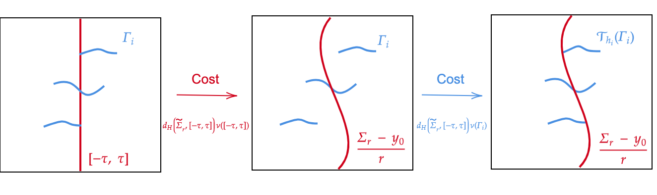
Figure 1. Transportation argument for the construction of a recovery sequence in the $\Gamma$ convergence of $(F_{r})_{r>0}$.

Theorem 6.1.

The family of functionals ${\left(F_{r}\right)}_{r>0}$ $\Gamma$-converges to $F$.

Proof.

$\Gamma$-liminf: we consider an infinitesimal sequence $(r_{n})_{n\in\mathbb{N}}$ such that ${(\nu_{n})}_{n\in\mathbb{N}}$ converges to $\nu$ in the weak sense, and that $\liminf_{n\to\infty}F_{r_{n}}(\nu_{n})<\infty$ for all $n\in\mathbb{N}$ (or at least for a subsequence), otherwise there is nothing to prove.

First we look at the first marginals in the definition of $F_{r_{n}}$. From the blow-up of $\sigma_{r}$ and the choice of $y_{0}$ as Lebesgue point of the density, (6.4) and (6.2), it follows that the renormalized measures $\bar{\sigma}_{r_{n}}\xrightharpoonup[n\to\infty]{\star}\sigma^{y_{0}}$.

By lower semi-continuity of the Wasserstein distance w.r.t. the narrow convergence, if we prove that $F(\nu)<\infty$, that is if the limit satisfies the constraints in the definition of $F$, we will have that

$$F(\nu)\leq\liminf_{n\to\infty}F_{r_{n}}(\nu_{n}).$$

As $\alpha\nu_{n}\geq\mathcal{H}^{1}\mathbin{\vrule height=6.88889pt,depth=0.0pt,width=0.55974pt\vrule height=0.55974pt,depth=0.0pt,width=5.59721pt}\Gamma_{n}$ for some $\Gamma_{n}\subset B_{1}(0)$ such that $r_{n}^{-1}(\Sigma-y_{0})\cup\Gamma_{n}\in\mathcal{A}$, Blaschke’s Theorem [3, Thm. 6.1] and the blow up of $\Sigma$ in Lemma 2.5 imply that, up to a subsequence, $\Gamma_{n}\xrightarrow[n\to\infty]{d_{H}}\Gamma$ and $r_{n}^{-1}(\Sigma-y_{0})\xrightarrow[n\to\infty]{K}\mathbb{R}\tau$. Hence:

$$\Xi_{n}\stackrel{{\scriptstyle\mbox{\tiny def.}}}{{=}}\left(\frac{\Sigma-y_{0}}{r_{n}}\right)\cup\Gamma_{n}\xrightarrow[n\to\infty]{K}\Xi\stackrel{{\scriptstyle\mbox{\tiny def.}}}{{=}}\mathbb{R}\tau\cup\Gamma.$$

In addition, as $\Sigma\cup\Gamma_{n}$ is connected, $\Xi$ is connected, and since $\Gamma\subset B_{1}$, it follows that also $[-\tau,\tau]\cup\Gamma$ is connected and belongs to $\mathcal{A}$. The fact that $\mathop{\rm supp}\nu\subset[-\tau,\tau]\cup\Gamma$ comes from the weak convergence of $\nu_{r_{n}}$ to $\nu$. As this convergence takes place in a compact set it also holds that $\nu(B_{1}(0))=\displaystyle\lim_{n\to\infty}\nu_{r_{n}}(B_{1}(0))=2\theta(y_{0})$.

It only remains to verify the density constraints, $\alpha\nu\geq\mathcal{H}^{1}\mathbin{\vrule height=6.88889pt,depth=0.0pt,width=0.55974pt\vrule height=0.55974pt,depth=0.0pt,width=5.59721pt}\Gamma$ (to simplify, we assume that $\mathcal{H}^{1}(\mathbb{R}\tau\cap\Gamma)=0$, otherwise we can simply rename $\Gamma\setminus\mathbb{R}\tau$ as $\Gamma$). Although $\nu_{n}\geq\alpha\mathcal{H}^{1}\mathbin{\vrule height=6.88889pt,depth=0.0pt,width=0.55974pt\vrule height=0.55974pt,depth=0.0pt,width=5.59721pt}\Gamma_{n}$, we cannot apply Golab’s Theorem to $\nu_{n}$ since we do not have an upper bound on the number of connected components of $\Gamma_{n}$.

What we do know is that the sequence $\Xi_{n}=\displaystyle r_{n}^{-1}(\Sigma-y_{0})\cup\Gamma_{n}$ satisfies the assumptions of Theorem 2.2. So we consider the measures $\alpha^{-1}\mathcal{H}^{1}\mathbin{\vrule height=6.88889pt,depth=0.0pt,width=0.55974pt\vrule height=0.55974pt,depth=0.0pt,width=5.59721pt}\Sigma+\nu_{n}^{\prime}\geq\alpha^{-1}\mathcal{H}^{1}\mathbin{\vrule height=6.88889pt,depth=0.0pt,width=0.55974pt\vrule height=0.55974pt,depth=0.0pt,width=5.59721pt}(\Sigma\cup\Gamma_{n})$ and analyse their blow up sequences. We know that

$$\mathcal{H}^{1}\mathbin{\vrule height=6.88889pt,depth=0.0pt,width=0.55974pt\vrule height=0.55974pt,depth=0.0pt,width=5.59721pt}\left(\frac{\Sigma-y_{0}}{r_{n}}\right)+\alpha\nu_{n}\geq\mathcal{H}^{1}\mathbin{\vrule height=6.88889pt,depth=0.0pt,width=0.55974pt\vrule height=0.55974pt,depth=0.0pt,width=5.59721pt}\left(\frac{\Sigma-y_{0}}{r_{n}}\cup\Gamma_{n}\right),$$

where the left hand side converges weakly to $\alpha^{-1}\mathcal{H}^{1}\mathbin{\vrule height=6.88889pt,depth=0.0pt,width=0.55974pt\vrule height=0.55974pt,depth=0.0pt,width=5.59721pt}\mathbb{R}\tau+\nu$ and for the right hand side we can extract a convergent subsequence. This is true since $y_{0}$ is a rectifiability point hence the part $\displaystyle\mathcal{H}^{1}\mathbin{\vrule height=6.88889pt,depth=0.0pt,width=0.55974pt\vrule height=0.55974pt,depth=0.0pt,width=5.59721pt}r_{n}^{-1}\left(\Sigma-y_{0}\right)$ converges to the approximate tanget space; the remaining mass $\displaystyle\mathcal{H}^{1}\mathbin{\vrule height=6.88889pt,depth=0.0pt,width=0.55974pt\vrule height=0.55974pt,depth=0.0pt,width=5.59721pt}\Gamma_{n}$ is bounded. Hence,assuming that the RHS converges in the weak-$\star$ sense to $\lambda$, Golab’s Theorem 2.2 implies that $\lambda\geq\alpha^{-1}\mathcal{H}^{1}\mathbin{\vrule height=6.88889pt,depth=0.0pt,width=0.55974pt\vrule height=0.55974pt,depth=0.0pt,width=5.59721pt}(\mathbb{R}\tau\cup\Gamma)$. We conclude that $\mathcal{H}^{1}\mathbin{\vrule height=6.88889pt,depth=0.0pt,width=0.55974pt\vrule height=0.55974pt,depth=0.0pt,width=5.59721pt}\mathbb{R}\tau+\alpha\nu\geq\mathcal{H}^{1}\mathbin{\vrule height=6.88889pt,depth=0.0pt,width=0.55974pt\vrule height=0.55974pt,depth=0.0pt,width=5.59721pt}(\mathbb{R}\tau\cup\Gamma),$ and therefore

$$\alpha\nu\geq\mathcal{H}^{1}\mathbin{\vrule height=6.88889pt,depth=0.0pt,width=0.55974pt\vrule height=0.55974pt,depth=0.0pt,width=5.59721pt}\Gamma.$$

$\Gamma$-limsup: The strategy to prove the limsup is illustrated in Figure 1, and roughly explained as follows. Given some $\nu$ such that $F(\nu)<\infty$ and the corresponding $\Gamma$, first we transport the mass over $[-\tau,\tau]$ to a measure supported over the set $\Sigma_{r}\stackrel{{\scriptstyle\mbox{\tiny def.}}}{{=}}r^{-1}(\Sigma-y_{0})$. Then, if $\Gamma$ already touches $(\Sigma-y_{0})/r$, we don’t need to do anything and let $\Gamma_{r}=\Gamma$. Otherwise, we translate $\Gamma$ (and the measure $\nu\mathbin{\vrule height=6.88889pt,depth=0.0pt,width=0.55974pt\vrule height=0.55974pt,depth=0.0pt,width=5.59721pt}\Gamma$) until it touches $\Sigma_{r}$, in order to preserve connectedness. Luckily, these transportation operations are of order $d_{H}([-\tau,\tau],\Sigma_{r})$, which goes to zero, from 2.5. Hence, the family of measures obtained will converge to $\nu$ and have finite $F_{r}$ energy.

To be more precise, given $\nu$ such that $F(\nu)<+\infty$, then it has a support of the form:

$$\mathop{\rm supp}\nu\subset S=[-\tau,\tau]\cup\bigcup_{i\in\mathbb{N}}\Gamma_{i},$$

where ${\left(\Gamma_{i}\right)}_{i\in\mathbb{N}}$ is the set of pairwise disjoint connected components of $S\setminus[-\tau,\tau]$ and $\alpha\nu\mathbin{\vrule height=6.88889pt,depth=0.0pt,width=0.55974pt\vrule height=0.55974pt,depth=0.0pt,width=5.59721pt}\Gamma_{i}\geq\mathcal{H}^{1}\mathbin{\vrule height=6.88889pt,depth=0.0pt,width=0.55974pt\vrule height=0.55974pt,depth=0.0pt,width=5.59721pt}\Gamma_{i}$.

Let us start by handling the mass over $\nu_{\tau}:=\nu\mathbin{\vrule height=6.88889pt,depth=0.0pt,width=0.55974pt\vrule height=0.55974pt,depth=0.0pt,width=5.59721pt}[-\tau,\tau]$. It suffices to transport it to a nonnegative measure supported on $\displaystyle\Sigma_{r_{n}}$. To this aim, we consider $P_{n}$ any measurable selection of the projection $\Pi_{\Sigma_{r_{n}}}$. By definition of the Hausdorff distance, for any $x\in[-\tau,\tau]$,

$$|x-P_{n}(x)|^{p}=\mathop{\rm dist}\left(x,\Sigma_{r_{n}}\right)^{p}\leq d_{H}\left([-\tau,\tau],\Sigma_{r_{n}}\right)^{p}.$$

So the Wasserstein distance between the measures ${P_{n}}_{\sharp}\nu_{\tau}$ and $\nu_{\tau}$ can be bounded from above by

$$W_{p}^{p}(\nu_{\tau},{P_{n}}_{\sharp}\nu_{\tau})\leq\int_{[-\tau,\tau]}\mathop{\rm dist}\left(x,\Sigma_{r_{n}}\right)^{p}{\rm d}\nu_{\tau}\leq d_{H}\left([-\tau,\tau],\Sigma_{r_{n}}\right)^{p}\nu([-\tau,\tau])\xrightarrow[n\to\infty]{}0,$$

as $\Sigma_{r}$ converges to $[-\tau,\tau]$ in the Hausdorff sense.

Next we translate the mass over the connected components $\Gamma_{i}$ until they touch $\Sigma_{r_{n}}$. Let $h\in\mathbb{R}^{d}$ and define the translation map $\mathcal{T}_{h}:\mathbb{R}^{d}\ni x\mapsto x-h$. Then for a given measure $\nu$ supported on $\Gamma$, it holds that $\mathop{\rm supp}\left({\mathcal{T}_{h}}_{\sharp}\nu\mathbin{\vrule height=6.88889pt,depth=0.0pt,width=0.55974pt\vrule height=0.55974pt,depth=0.0pt,width=5.59721pt}\Gamma\right)=\mathcal{T}_{h}(\Gamma).$

So, if $\Gamma_{i}\cap\Sigma_{r_{n}}=\emptyset$, as the set $[-\tau,\tau]\cup\Gamma$ is connected, we consider some point $y_{i}\in[-\tau,\tau]\cap\Gamma_{i}$ and we take $h_{i}$, with minimal norm such that $y_{i}-h_{i}\in\Sigma_{r_{n}}$. But then by definition, $|h_{i}|=d\left(y_{i},\Sigma_{r_{n}}\right)$. And finally, estimating the Wasserstein distance we have that

$$W_{p}^{p}\left(\nu\mathbin{\vrule height=6.88889pt,depth=0.0pt,width=0.55974pt\vrule height=0.55974pt,depth=0.0pt,width=5.59721pt}\Gamma_{i},\mathcal{T}_{h_{i},\sharp}\nu\mathbin{\vrule height=6.88889pt,depth=0.0pt,width=0.55974pt\vrule height=0.55974pt,depth=0.0pt,width=5.59721pt}\Gamma_{i}\right) \leq\int_{\Gamma_{i}}|y-\mathcal{T}_{h_{i}}(y)|^{p}{\rm d}\nu=|h_{i}|^{p}\nu(\Gamma_{i})$$

$$\leq d_{H}([-\tau,\tau],\Sigma_{r_{n}})^{p}\nu(\Gamma_{i})$$

Therefore, defining a map $T_{n}$ as follows

$$T_{n}(y):=\left\{\begin{array}[]{cc}P_{n}(y),&\text{ if $y\in[-\tau,\tau]$,}\\ \mathcal{T}_{h_{i}}(y),&\text{ if $y\in\Gamma_{i}$}\end{array}\right.$$

we see that if $\nu_{n}:={T_{n}}_{\sharp}\nu$,

$$W_{p}^{p}\left(\nu,\nu_{n}\right)\leq d_{H}^{p}([-\tau,\tau],\Sigma_{r_{n}})\left(\nu([-\tau,\tau])+\sum_{i\in\mathbb{N}}\nu(\Gamma_{i})\right)\xrightarrow[r_{n}\to 0]{}0$$

and in particular $\nu_{n}\rightharpoonup\nu$. Finally, we get $\nu_{n}(B_{1}(0))=\nu(B_{1}(0))=2\theta_{\delta}(y_{0})$ and we conclude that $F_{r_{n}}(\nu_{n})<\infty$, for all $n\in\mathbb{N}$. By the continuity of the Wasserstein distance with respect to the weak convergence, we have that:

$$F_{r_{n}}(\nu_{n})\xrightarrow[n\to\infty]{}F(\nu).$$

The $\Gamma$-convergence follows. ∎

Now that we have characterized the limit problem, we show that the optimal transportation is given by projections as the blow-up family.

Lemma 6.2.

The optimal transportation plan between $\sigma^{y_{0}}$ and $\lambda^{y_{0}}=\theta_{\delta}(y_{0})\mathcal{H}^{1}\mathbin{\vrule height=6.88889pt,depth=0.0pt,width=0.55974pt\vrule height=0.55974pt,depth=0.0pt,width=5.59721pt}[-\tau,\tau]$ is unique and given by the projection map $\Pi_{[-\tau,\tau]}$.

Proof.

Consider a family $\bar{\gamma}_{r}$ of optimal transportation plans from $\bar{\sigma}_{r}$ to $\bar{\nu}_{r}$. Up to a subsequence it converges to some $\bar{\gamma}^{y_{0}}$, which, by the stability of optimal transportation plans, also transports $\sigma^{y_{0}}$ to $\lambda^{y_{0}}$ optimally. Since $\bar{\sigma}_{r},\bar{\nu}_{r}$ are generated by the pushforward of $\nu_{\text{exc}}\mathbin{\vrule height=6.88889pt,depth=0.0pt,width=0.55974pt\vrule height=0.55974pt,depth=0.0pt,width=5.59721pt}B_{r}(y_{0})$ by $\Phi^{y_{0},r}$, from Lemma 5.1 we know that

$$\mathop{\rm supp}\bar{\gamma}_{r}\subset\text{graph}\left(\Pi_{\Sigma_{r}}\right).$$

Let us show that $\mathop{\rm supp}\bar{\gamma}^{y_{0}}\subset\text{graph}\left(\Pi_{[-\tau,\tau]}\right)$. Indeed if $(x,p)\in\mathop{\rm supp}\bar{\gamma}^{y_{0}}$, there is an open ball $B$ centered at $(x,p)$ such that

$$0<\bar{\gamma}^{y_{0}}(B)\leq\liminf_{r\to 0}\bar{\gamma}_{r}(B).$$

In particular, we can find $\mathop{\rm supp}\bar{\gamma}_{r}\ni(x_{r},p_{r})\xrightarrow[r\to 0]{}(x,p)$. So it holds that

$$|x-p|=\lim_{r\to 0}|x_{r}-p_{r}|=\lim_{r\to 0}\mathop{\rm dist}\left(x_{r},\Sigma_{r}\right)=\mathop{\rm dist}(x,[-\tau,\tau]),$$

where the last equality comes from the uniform convergence of the distance functions, recalling from Lemma 2.5 that $\Sigma_{r}\xrightarrow[r\to 0]{d_{H}}[-\tau,\tau]$.

Now we show that this property is true for any other optimal plan. Consider $\gamma^{y_{0}}$ transporting $\sigma^{y_{0}}$ to $\lambda^{y_{0}}$ optimaly, then by the optimality of $\bar{\gamma}^{y_{0}}$ it holds that

$$\int_{\mathbb{R}^{d}}(\mathop{\rm dist}(x,[-\tau,\tau]))^{p}{\rm d}\sigma^{y_{0}} =\int|x-y|^{p}{\rm d}\bar{\gamma}^{y_{0}}=\int|x-y|^{p}{\rm d}\gamma^{y_{0}}$$

$$\geq\int(\mathop{\rm dist}(x,[-\tau,\tau]))^{p}{\rm d}\gamma^{y_{0}}=\int_{\mathbb{R}^{d}}\mathop{\rm dist}(x,[-\tau,\tau])^{p}{\rm d}\sigma^{y_{0}}.$$

Since $|x-y|-\mathop{\rm dist}(x,[-\tau,\tau])\geq 0$ for $\gamma^{y_{0}}$-a.e. $(x,y)$ and the inequality above must be an equality, we must have $\mathop{\rm supp}\gamma^{y_{0}}\subset\text{graph}\left(\Pi_{[-\tau,\tau]}\right)$ for any optimal $\gamma^{y_{0}}$. In particular, as $\Pi_{[-\tau,\tau]}$ is univalued, it means that the optimal transportation plan is unique and given by the projection map. ∎

6.2. Competitor for the limit problem in 2D

In this section we restrict the discussion to $\mathbb{R}^{2}$ and obtain a contradiction to the fact that the exceeding density $\theta_{\delta}$ is not zero by building a better competitor to the minimization of the $\Gamma$ limit.

From the $\Gamma$-convergence Theorem 6.1 we know that

$$\lambda^{y_{0}}\stackrel{{\scriptstyle\mbox{\tiny def.}}}{{=}}\theta_{\delta}(y_{0})\mathcal{H}^{1}\mathbin{\vrule height=6.88889pt,depth=0.0pt,width=0.55974pt\vrule height=0.55974pt,depth=0.0pt,width=5.59721pt}[-\tau,\tau]\in\mathop{\rm argmin}F,$$

where $F$ is defined in (6.8). If we are able to construct another competitor with a stricly smaller energy $F$, we obtain a contradiction to the existence of points such that $\theta_{\delta}(y_{0})>0$. Without loss of generality, we assume that $\tau=e_{2}$ where $(e_{1},e_{2})$ is the canonical basis of $\mathbb{R}^{2}$.

We propose a new transportation strategy consisting in sending the mass, that was first projected onto a vertical segment, to a horizontal line as in Figure 2. To obtain a smaller transportation cost with this strategy we need to distinguish the mass that comes from each side of $[-e_{2},e_{2}]$. Hence we decompose $\sigma^{y_{0}}=\sigma_{+}+\sigma_{-}$ with $\mathop{\rm supp}\sigma_{\pm}\subset\{\pm x_{1}\geq\delta\}$, and $\Pi_{[-e_{2},e_{2}]}{}_{\sharp}\sigma_{\pm}=\theta_{\pm}\mathcal{H}^{1}\mathbin{\vrule height=6.88889pt,depth=0.0pt,width=0.55974pt\vrule height=0.55974pt,depth=0.0pt,width=5.59721pt}[-e_{2},e_{2}]$ for $\theta_{\pm}\geq 0$, $\theta_{+}+\theta_{-}=\theta_{\delta}(y_{0})$.

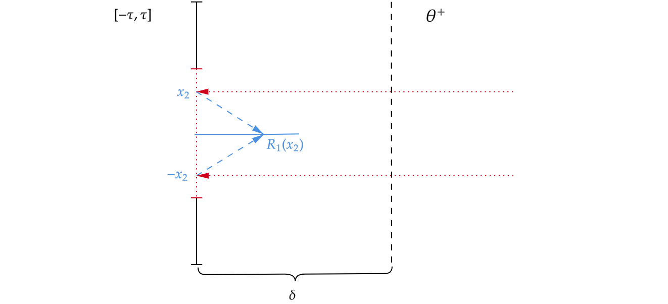
Figure 2. Construction of the better competitor to the minimization of the functional $F$.

Theorem 6.3.

Let $\rho_{0}\in\mathcal{P}_{p}(\mathbb{R}^{2})$ such that $\rho_{0}\ll\mathcal{H}^{1}$ and suppose that the parameter $\Lambda<\Lambda_{\star}$. Then the solution to the relaxed problem ($\overline{P}_{\Lambda}$) is of the form

$$\nu=\mathcal{L}(\nu)^{-1}\mathcal{H}^{1}\mathbin{\vrule height=6.88889pt,depth=0.0pt,width=0.55974pt\vrule height=0.55974pt,depth=0.0pt,width=5.59721pt}\Sigma+\rho_{\text{exc}}\mathbin{\vrule height=6.88889pt,depth=0.0pt,width=0.55974pt\vrule height=0.55974pt,depth=0.0pt,width=5.59721pt}\Sigma,$$

where $\rho_{\text{exc}}$ was defined in (5.4).

In addition, if $\rho_{0}$ does not give mass to $1$-rectifiable sets the shape optimization problem ($P_{\Lambda}$) admits a solution.

In particular, point (2) of Theorem 1.1 follows.

Proof.

First we recall the decomposition of $\nu_{\text{exc}}$ in (5.15) to write the solution as

$$\nu=\nu_{\mathcal{H}^{1}}+\sup_{\delta>0}\nu_{\delta}+\rho_{\text{exc}}\mathbin{\vrule height=6.88889pt,depth=0.0pt,width=0.55974pt\vrule height=0.55974pt,depth=0.0pt,width=5.59721pt}\Sigma.$$

To prove the first point, our goal is to show that $\nu_{\delta}\equiv 0$. Fix some $\delta>0$, from the hypothesis that $\rho_{0}\ll\mathcal{H}^{1}$ we know that $\nu_{\delta}=\theta_{\delta}\mathcal{H}^{1}\mathbin{\vrule height=6.88889pt,depth=0.0pt,width=0.55974pt\vrule height=0.55974pt,depth=0.0pt,width=5.59721pt}\Sigma$ is rectifiable. So we can perform the blow-up procedure described in Section 6.1 around a point such that $\theta_{\delta}(y_{0})>0$. We also recall the decomposition of the blow-up limits

$$\sigma^{y_{0}}=\sigma_{+}+\sigma_{-},\quad\lambda^{y_{0}}=(\theta_{+}+\theta_{-})\mathcal{H}^{1}\mathbin{\vrule height=6.88889pt,depth=0.0pt,width=0.55974pt\vrule height=0.55974pt,depth=0.0pt,width=5.59721pt}[-\tau,\tau],\text{ s.t. }\theta_{+}(\cdot)+\theta_{-}(\cdot)=\theta_{\delta}(y_{0})>0$$

where $\sigma_{\pm}$ form $\theta_{\pm}\mathcal{H}^{1}\mathbin{\vrule height=6.88889pt,depth=0.0pt,width=0.55974pt\vrule height=0.55974pt,depth=0.0pt,width=5.59721pt}[-\tau,\tau]$ and $\lambda^{y_{0}}\in\mathop{\rm argmin}F$, defined in (6.8).

Take some $z\in(-\tau,\tau)$ that is a Lebesgue point of $\theta_{+}$ such that $\theta_{+}(z)>0$. We assume for simplicity of notation that $z=0$, but the following argument can be easily adapted to any $z$. From Lemma 6.2, the optimal transportation of $\sigma_{+}$ to $\theta_{+}\mathcal{H}^{1}\mathbin{\vrule height=6.88889pt,depth=0.0pt,width=0.55974pt\vrule height=0.55974pt,depth=0.0pt,width=5.59721pt}[-\tau,\tau]$ is given by the projection map. So given $\varepsilon>0$ we consider the alternative transportation map

$$R(x)=\begin{cases}(R_{1}(x),0)&\mbox{if $x_{1}\geq\delta$, $0\leq|x_{2}|\leq\varepsilon$}\\ (0,x_{2})&\mbox{otherwise,}\end{cases}$$

where $R_{1}(x)$ is determined by conservation of mass

$$\int_{-|x_{2}|}^{|x_{2}|}\theta_{+}(t){\rm d}t=\frac{1}{\alpha}\int_{0}^{R_{1}(x)}{\rm d}t,\text{ so that }R_{1}(x)=\alpha\int_{-|x_{2}|}^{|x_{2}|}\theta_{+}(t){\rm d}t.$$

In other words, the mass that was sent to the vertical segment $\{0\}\times[-|x_{2}|,|x_{2}|]$ is now sent to the horizontal segment $[0,R_{1}(x)]\times\{0\}$, this construction is illustrated in Figure 2. Setting $\ell_{\varepsilon}=\int_{-\varepsilon}^{\varepsilon}\theta_{+}(t){\rm d}t$, this operation forms the measure $\alpha^{-1}\mathcal{H}^{1}\mathbin{\vrule height=6.88889pt,depth=0.0pt,width=0.55974pt\vrule height=0.55974pt,depth=0.0pt,width=5.59721pt}[0,\ell_{\varepsilon}]$, hence satisfying the density constraints.

Next we choose $\varepsilon$ small enough to ensure a smaller transportation cost. For this it suffices that for all $x=(x_{1},x_{2})$ such that $x_{1}\geq\delta$ and $|x_{2}|\leq\varepsilon$ we have that

(6.9) $$\left\lvert x-(0,x_{2})\right\rvert^{2}>\left\lvert x-R(x)\right\rvert^{2} \Longleftrightarrow x_{1}^{2}>(x_{1}-R_{1}(x))^{2}+x_{2}^{2}$$

(6.10) $$\Longleftrightarrow R_{1}(x)\left(2x_{1}-R_{1}(x)\right)>x_{2}^{2}.$$

Fix $\varepsilon$ small enough so that for all such $x$

• $\displaystyle\alpha\int_{-\varepsilon}^{\varepsilon}\theta_{+}(t){\rm d}t<\delta$,

• $\displaystyle\int_{-|x_{2}|}^{|x_{2}|}\theta_{+}(t){\rm d}t\geq|x_{2}|\theta_{+}(0)$ if $0<|x_{2}|<\varepsilon$, since $0$ is a Lebesgue point of $\theta_{+}$,

• $\varepsilon<\delta\alpha\theta_{+}(0)$.

For this choice of $\varepsilon$ for any $0<|x_{2}|\leq\varepsilon$ and $x_{1}\geq\delta$ we verify that

$$x_{2}^{2} \leq\varepsilon|x_{2}|<\delta\alpha\theta_{+}(0)|x_{2}|\leq\delta\alpha\int_{-|x_{2}|}^{|x_{2}|}\theta_{+}(t){\rm d}t=\delta R_{1}(x)=2\delta R_{1}(x)-\delta R_{1}(x)$$

$$\leq R_{1}(x)\left(2x_{1}-R_{1}(x)\right),$$

where in the last inequality we use the fact that $x_{1}\geq\delta$ and $R_{1}(x)\leq\delta$ for all $x$. Therefore (6.10) is verifed and we conclude that $W_{p}^{p}(\sigma_{+},R_{\sharp}\sigma_{+})<W_{p}^{p}(\sigma_{+},\lambda_{+}).$

This contradicts the fact that $\theta_{\delta}\mathcal{H}^{1}\mathbin{\vrule height=6.88889pt,depth=0.0pt,width=0.55974pt\vrule height=0.55974pt,depth=0.0pt,width=5.59721pt}[-\tau,\tau]$ is a minimizer of $F$, so for $\mathcal{H}^{1}$-a.e. $z$ we have $\theta_{+}(z)=\theta_{-}(z)=0$. We conclude that $\nu_{\delta}\equiv 0$ and hence

$$\nu=\nu_{\mathcal{H}^{1}}+\rho_{\text{exc}}\mathbin{\vrule height=6.88889pt,depth=0.0pt,width=0.55974pt\vrule height=0.55974pt,depth=0.0pt,width=5.59721pt}\Sigma,$$

proving the first characterization of the solutions.

In particular, if $\rho_{0}$ does not give mass to $1$D sets, neither does $\rho_{\text{exc}}$ since $\rho_{\text{exc}}\ll\rho_{0}$. So $\nu_{\text{exc}}\equiv 0$ and the solution must be uniformly distributed over $\Sigma$, being therefore a solution to the original problem ($P_{\Lambda}$). ∎

7. Ahlfors regularity

In this section we prove that whenever the initial measure $\rho_{0}\in L^{\frac{d}{d-1}}(\mathbb{R}^{d})$, the optimal solutions to the relaxed problem ($\overline{P}_{\Lambda}$) have an Ahlfors regular support.

Definition 7.1.

We say that a set $\Sigma\subset\mathbb{R}^{d}$ is Ahlfors regular whenever there exist $r_{0}>0$ and $c,C>0$ such that for $r\leq r_{0}$ it holds that

$$cr\leq\mathcal{H}^{1}(\Sigma\cap B_{r}(x))\leq Cr,\text{ for all $x\in\Sigma$.}$$

We prove in this section the following result.

Theorem 7.1.

If $\rho_{0}\in L^{\frac{d}{d-1}}(\mathbb{R}^{d})$, let $\nu$ be a solution of the relaxed problem ($\overline{P}_{\Lambda}$) and $\Sigma$ its support. Then $\Sigma$ is Ahlfors-regular, there exist $r_{0}>0$ depending on $d,p,\rho_{0}$ and $\alpha$ and $\bar{C}>0$ depending only on $d$ and $p$ such that, for all $\bar{x}\in\Sigma$ and $r\leq r_{0}$,

$$r\leq\mathcal{H}^{1}(\Sigma\cap B_{r}(\bar{x}))\leq\bar{C}r.$$

The lower bound (with $c=1$ and $r_{0}=\mathop{\rm diam}\Sigma$) follows directly from the connectedness of $\Sigma$, hence we skip the proof. The upper bound will follow as a corollary of Lemma 7.2 below. Let us describe the strategy for proving this estimate.

The idea is similar to proving the $L^{\infty}$ bound on the excess measure: if in a small ball $B_{r}(\bar{x})$ the measure $\nu$ has too much mass, we build another “closer” 1D structure onto which the mass is transfered at a smaller cost. Yet there is an additional difficulty: when replacing $\Sigma\cap B_{r}(\bar{x})$ with another set we should preserve connectedness. In 5.4, we were rearranging only the excess mass and it was not an issue. It means we now need to control the number of connected components of $\Sigma\setminus B_{r}(\bar{x})$ and find a way to connect them back without adding too much length.

This number of connected components is controlled by the quantity $\mathcal{H}^{0}(\Sigma\cap\partial B_{r}(\bar{x}))$, which we can control on average by means of the generalized area formula [3, Theorem 2.91]: If $f:\mathbb{R}^{M}\to\mathbb{R}^{N}$ is a Lipschitz function and $E\subset\mathbb{R}^{M}$ is a $k$-rectifiable set then it holds that

(7.1) $$\int_{\mathbb{R}^{N}}\mathcal{H}^{0}(E\cap f^{-1}(y)){\rm d}\mathcal{H}^{k}(y)=\int_{E}J_{k}{\rm d}^{E}f_{x}{\rm d}\mathcal{H}^{k}(x),$$

where ${\rm d}^{E}f_{x}$ is the restriction of $\nabla f(x)$ (when $f$ is smooth) to the approximate tangent space of $E$. Hence, choosing $E=\Sigma\cap(B_{r_{1}}(\bar{x})\setminus B_{r_{2}}(\bar{x}))$ and $f:x\mapsto|x-\bar{x}|$, we deduce from (7.1) that

(7.2) $$\int_{r_{2}}^{r_{1}}\mathcal{H}^{0}(\Sigma\cap\partial B_{s}(\bar{x})){\rm d}s\leq\mathcal{H}^{1}(\Sigma\cap B_{r_{1}}(\bar{x}))-\mathcal{H}^{1}(\Sigma\cap B_{r_{2}}(\bar{x}))$$

Using this we first prove the following lemma:

Lemma 7.2.

Assume $\rho_{0}\in L^{\frac{d}{d-1}}(\mathbb{R}^{d})$. There exist $\bar{C}(d,p)>0$ and $r_{0}$ depending on $\rho_{0}$, $\alpha$, $d$, $p$, such that for any $C\geq\bar{C}$, if $r\leq r_{0}$ and $x\in\Sigma$, then either $\mathcal{H}^{1}(\Sigma\cap B_{r}(x))\leq Cr$ or $\mathcal{H}^{1}(\Sigma\cap B_{2r}(x))\geq 10Cr$.

Proof.

Let $r>0$ and $C\geq 1$, and let $\bar{x}\in\Sigma$ such that both $\mathcal{H}^{1}(\Sigma\cap B_{r}(\bar{x}))>Cr$ and $\mathcal{H}^{1}(\Sigma\cap B_{2r}(\bar{x}))<10Cr$. We show that if $r\leq r_{0}$ and $C\geq\bar{C}$, which will both be chosen later, then we can contruct a better competitor to the minimizer $\nu$.

The function $f:s\mapsto\mathcal{H}^{1}(\Sigma\cap B_{s}(\bar{x}))$ is nondecreasing, hence in $BV(\mathbb{R}_{+})$ and satisfies, thanks to (7.2), that $\mathcal{H}^{0}(\Sigma\cap\partial B_{s}(\bar{x})){\rm d}s\leq Df$ in the sense of measures (equivalently, $\mathcal{H}^{0}(\Sigma\cap\partial B_{s}(\bar{x})$ is less than, or equal to $\tilde{D}f$, the absolutely continuous part of $Df$).

We note that

$$\mathop{\rm inf}_{s\in(3r/2,2r)}\left(\frac{s\mathcal{H}^{0}\left(\Sigma\cap\partial B_{s}(\bar{x})\right)}{\mathcal{H}^{1}(\Sigma\cap B_{s}(\bar{x}))}\right) \leq\frac{2}{r}\int_{3r/2}^{2r}\frac{s\mathcal{H}^{0}\left(\Sigma\cap\partial B_{s}(\bar{x})\right)}{\mathcal{H}^{1}(\Sigma\cap B_{s}(\bar{x}))}ds$$

$$\leq 4\int_{3r/2}^{2r}\frac{1}{f(s)}\tilde{D}f(s){\rm d}s$$

$$\leq 4\ln\left(\frac{f(2r)}{f(3r/2)}\right),$$

where we have used the classical chain rule at almost every point and [3, Cor. 3.29]. Since $f(2r)/f(3r/2)<(10Cr)/(Cr)=10$, we deduce that there exists $\bar{s}\in(3r/2,2r)$ such that

(7.3) $$\bar{\delta}\bar{s}\mathcal{H}^{0}(\Sigma\cap\partial B_{\bar{s}}(\bar{x}))\leq\mathcal{H}^{1}(\Sigma\cap B_{\bar{s}}(\bar{x}))\quad\mbox{ where $\bar{\delta}:=\frac{1}{4\ln 10}.$}$$

Now, we let

(7.4) $$M=2\left(1+10\cdot\left(\frac{40}{17}\right)^{p-1}\right)$$

(this choice will be made clear at the end of this proof) and we consider

(7.5) $$\delta:=\frac{\bar{\delta}}{10M}<\bar{\delta}<\frac{1}{2}.$$

We define a set $\Gamma$ as follows: we choose a finite covering of $\partial B_{1}(0)$ with balls $B(x_{i},\delta/2)$ centered at points $(x_{i})_{i=1}^{N}$ (the minimal number $N$ depends only on $d$ and $p$, through $\delta$). Then, we find a minimal tree connecting the points $(x_{i})_{i=1}^{N}$ through geodesics on the sphere. We add to this minimal tree the segments $[x_{i},(1+\delta)x_{i}]$, $i=1,\dots,N$. We call $\Gamma$ the resulting (connected) set, whose total length $L\stackrel{{\scriptstyle\mbox{\tiny def.}}}{{=}}\mathcal{H}^{1}(\Gamma)$ is of order at most $2N\delta$ and depends only on $d$ and $p$. Notice that each point of $\partial B_{1}$ is at distance at most $\delta$, along the geodesic curve on the sphere, to a point of $\Gamma$, and that thanks to the “spikes” $[x_{i},(1+\delta)x_{i}]$, any point with, say, $|x|\geq 10$ is closer to a point of $\Gamma$ than from any point in $B_{1}(0)$.

Now, we define

$$\Gamma_{\bar{s}}\stackrel{{\scriptstyle\mbox{\tiny def.}}}{{=}}(\bar{x}+\bar{s}\Gamma)\cup\bigcup_{x\in\Sigma\cap\partial B_{\bar{s}}}S_{x},$$

where $S_{x}$ denotes a geodesic connecting $x$ to $\bar{x}+\bar{s}\Gamma$, of length at most $\mathcal{H}^{1}(S_{x})\leq\bar{s}\delta$. Since $\bar{s}<2r$ and $\delta<1/2$, it follows that $\Gamma_{\bar{s}}\subset B_{3r}(\bar{x})$. We define the competitor set as

$$\Sigma^{\prime}\stackrel{{\scriptstyle\mbox{\tiny def.}}}{{=}}\Sigma\setminus B_{\bar{s}}(\bar{x})\cup\Gamma_{\bar{s}}.$$

The addition of the geodesics $S_{x}$ ensures that $\Sigma^{\prime}$ remains connected, and using (7.3), we estimate the length of $\Gamma_{\bar{s}}$ as

(7.6) $$\mathcal{H}^{1}(\Gamma_{\bar{s}}) \leq L\bar{s}+\delta\bar{s}\mathcal{H}^{0}(\Sigma\cap\partial B_{\bar{s}}(\bar{x}))\leq 2Lr+\tfrac{1}{10M}\mathcal{H}^{1}(\Sigma\cap B_{\bar{s}}(\bar{x}))$$

$$<(2L+\tfrac{C}{M})r,$$

Now we define a new competitor $\nu^{\prime}$ whose support is $\Sigma^{\prime}$. If $\gamma$ denotes the optimal transportation plan from $\rho_{0}$ to $\nu$, given $s>0$ let

$$\rho_{s}\stackrel{{\scriptstyle\mbox{\tiny def.}}}{{=}}{\pi_{0}}_{\sharp}\left(\gamma\mathbin{\vrule height=6.88889pt,depth=0.0pt,width=0.55974pt\vrule height=0.55974pt,depth=0.0pt,width=5.59721pt}\left(\mathbb{R}^{d}\times B_{s}\right)\right)$$

denote the portion of the measure $\rho_{0}$ which is transported to the ball $B_{s}$. In particular, the above length estimates imply that

(7.7) $$Lr\leq\mathcal{H}^{1}(\Gamma_{\bar{s}})<(2L+\tfrac{C}{M})r\leq(2\tfrac{L}{C}+\tfrac{1}{M})\alpha\nu(B_{r})\leq\alpha\rho_{r}(\mathbb{R}^{d})\leq\alpha\rho_{\bar{s}}(\mathbb{R}^{d}),$$

where $\alpha:=\mathcal{L}(\nu)$, and using that $M\geq 2$ (see (7.4)) and assuming $\bar{C}\geq 4L$ (which we recall depends only on $d$ and $p$). But, if $r$ is small enough (not depending on $\bar{x}$, by uniform equi-integrability of $\rho_{0}^{d/(d-1)}$) Holder’s inequality implies that

(7.8) $$\alpha\rho_{\bar{s}}(B_{10r}(\bar{x}))\leq\alpha\|\rho_{0}\|_{L^{\frac{d}{d-1}}(B_{10r}(\bar{x}))}|B_{10r}(\bar{x})|^{\frac{1}{d}}\leq Lr.$$

We fix $r_{0}>0$, which depends only on the dimension (through $L$), the integrability of $\rho_{0}$, and $\alpha$, such that the above inequality holds for $r\leq r_{0}$.

Equations (7.7)-(7.8) show that for $r$ small enough, part of the mass transported to $\nu\mathbin{\vrule height=6.88889pt,depth=0.0pt,width=0.55974pt\vrule height=0.55974pt,depth=0.0pt,width=5.59721pt}B_{\bar{s}}$ must come from outside of the ball $B_{10r}$. In particular, since $t\mapsto\rho_{\bar{s}}(B_{t}(\bar{x}))$ is continuous, there is $R>10r$ such that

(7.9) $$\rho_{\bar{s}}(B_{R}(\bar{x}))=\alpha^{-1}\mathcal{H}^{1}(\Gamma_{\bar{s}}).$$

To form the new competitor we use the following strategy: the mass sent to $\Sigma\setminus B_{\bar{s}}$ remains untouched, the mass $\rho_{\bar{s}}\mathbin{\vrule height=6.88889pt,depth=0.0pt,width=0.55974pt\vrule height=0.55974pt,depth=0.0pt,width=5.59721pt}B_{R}$ previously used to form $\nu\mathbin{\vrule height=6.88889pt,depth=0.0pt,width=0.55974pt\vrule height=0.55974pt,depth=0.0pt,width=5.59721pt}B_{\bar{s}}$ is transported to $\alpha^{-1}\mathcal{H}^{1}\mathbin{\vrule height=6.88889pt,depth=0.0pt,width=0.55974pt\vrule height=0.55974pt,depth=0.0pt,width=5.59721pt}\Gamma_{\bar{s}}$ and the remaining mass is projected onto $\Gamma_{\bar{s}}$.

So, letting $\tilde{\gamma}$ denote the optimal transportation plan between $\rho_{\bar{s}}\mathbin{\vrule height=6.88889pt,depth=0.0pt,width=0.55974pt\vrule height=0.55974pt,depth=0.0pt,width=5.59721pt}B_{R}$ and $\alpha^{-1}\mathcal{H}^{1}\mathbin{\vrule height=6.88889pt,depth=0.0pt,width=0.55974pt\vrule height=0.55974pt,depth=0.0pt,width=5.59721pt}\Gamma_{\bar{s}}$, define the new plan

$$\gamma^{\prime}=\gamma\mathbin{\vrule height=6.88889pt,depth=0.0pt,width=0.55974pt\vrule height=0.55974pt,depth=0.0pt,width=5.59721pt}\mathbb{R}^{d}\times B_{\bar{s}}(\bar{x})^{c}+\tilde{\gamma}\mathbin{\vrule height=6.88889pt,depth=0.0pt,width=0.55974pt\vrule height=0.55974pt,depth=0.0pt,width=5.59721pt}B_{R}\times\mathbb{R}^{d}+(\text{id},\pi_{\Gamma_{\bar{s}}})_{\sharp}\left(\rho_{\bar{s}}\mathbin{\vrule height=6.88889pt,depth=0.0pt,width=0.55974pt\vrule height=0.55974pt,depth=0.0pt,width=5.59721pt}B_{R}^{c}\right),$$

and the new competitor $\nu^{\prime}$ as its second marginal. By construction, $\alpha\nu^{\prime}\geq\mathcal{H}^{1}\mathbin{\vrule height=6.88889pt,depth=0.0pt,width=0.55974pt\vrule height=0.55974pt,depth=0.0pt,width=5.59721pt}\Sigma^{\prime}$ so that $\mathcal{L}(\nu^{\prime})\leq\mathcal{L}(\nu)$. We now estimate the gain in terms of transportation cost.

• For $(x,y)\in B_{R}\times B_{\bar{s}}$ and for any $y^{\prime}\in\Gamma_{\bar{s}}\subset B_{3r}$, as $\bar{s}\leq 2r$ and $10r<R$, the convexity of $t\mapsto t^{p}$ yields

  $$|x-y^{\prime}|^{p} \leq\left(|x-y|+5r\right)^{p}\leq|x-y|^{p}+5rp\left(|x-y|+5r\right)^{p-1}$$

  $$\leq|x-y|^{p}+5rp{{\left(2R\right)^{p-1}}}.$$

  Hence integrating w.r.t. the transportation plans we get

  $$\int_{B_{R}\times\Gamma_{\bar{s}}}|x-y^{\prime}|^{p}{\rm d}\tilde{\gamma}\leq\int_{B_{R}\times B_{\bar{s}}}|x-y|^{p}{\rm d}\gamma+5rp\left({2R}\right)^{p-1}\rho_{\bar{s}}\left(B_{R}\right),$$

  (this can be checked by disintegration w.r.t. their common first marginal, which is the measure $\rho_{\bar{s}}\mathbin{\vrule height=6.88889pt,depth=0.0pt,width=0.55974pt\vrule height=0.55974pt,depth=0.0pt,width=5.59721pt}B_{R}$).

• Similarly, for $x\in B_{R}^{c}$ and $y\in B_{\bar{s}}\setminus B_{r}$ the addition of the spikes ensures that

  $$|x-\pi_{\Gamma_{\bar{s}}}(x)|\leq|x-y|.$$

  However if $x\in B_{R}^{c}$ and $y\in B_{r}$ it holds that

  $$|x-\pi_{\Gamma_{\bar{s}}}(x)|\leq|x-y|-\frac{r}{2}\text{ and }|x-y|\geq R-r,$$

  so that once again using the convexity of $t\mapsto t^{p}$ we have

  $$|x-\pi_{\Gamma_{\bar{s}}}(x)|^{p} \leq\left(|x-y|-\frac{r}{2}\right)^{p}\leq|x-y|^{p}-p\frac{r}{2}\left(|x-y|-\frac{r}{2}\right)^{p-1}$$

  $$\leq|x-y|^{p}-p\frac{r}{2}\left(\frac{17}{20}R\right)^{p-1}.$$

  So, decomposing the integration for the points going to $B_{r}$ and to $B_{\bar{s}}\setminus B_{r}$, this time the transportation cost can be bound by:

  $$\int_{B_{R}^{c}}|x-\pi_{\Gamma_{\bar{s}}}(x)|^{p}{\rm d}\rho_{\bar{s}} =\int_{B_{R}^{c}}|x-\pi_{\Gamma_{\bar{s}}}(x)|^{p}{\rm d}(\rho_{\bar{s}}-\rho_{r})+\int_{B_{R}^{c}}|x-\pi_{\Gamma_{\bar{s}}}(x)|^{p}{\rm d}\rho_{r}$$

  $$\leq\int_{B_{R}^{c}\times B_{\bar{r}}}|x-y|^{p}{\rm d}\gamma-p\frac{r}{2}\left(\frac{17}{20}R\right)^{p-1}\rho_{r}\left(B_{R}^{c}\right).$$

We get:

$$W_{p}^{p}(\rho_{0},\nu^{\prime}) \leq W_{p}^{p}(\rho_{0},\nu)+5rp\left(2R\right)^{p-1}\rho_{\bar{s}}\left(B_{R}\right)-p\frac{r}{2}\left(\frac{17}{20}R\right)^{p-1}\rho_{r}\left(B_{R}^{c}\right).$$

As $\mathcal{L}(\nu^{\prime})\leq\mathcal{L}(\nu)$, the optimality of $\nu$ gives that $W_{p}^{p}(\rho_{0},\nu)\leq W_{p}^{p}(\rho_{0},\nu^{\prime})$, which, along with the previous estimates, implies

$$0\leq 5\cdot 2^{p-1}\rho_{\bar{s}}\left(B_{R}\right)-\frac{1}{2}\left(\frac{17}{20}\right)^{p-1}\rho_{r}\left(B_{R}^{c}\right)\ \Leftrightarrow\ \rho_{r}\left(B_{R}^{c}\right)\leq 10\cdot\left(\frac{40}{17}\right)^{p-1}\rho_{\bar{s}}\left(B_{R}\right).$$

On the other hand, since

$$\rho_{r}\left(B_{R}(\bar{x})^{c}\right)=\nu(B_{r})-\rho_{r}(B_{R}(\bar{x}))\geq\alpha^{-1}Cr-\rho_{r}(B_{R}(\bar{x}))\geq\alpha^{-1}Cr-\rho_{\bar{s}}(B_{R}(\bar{x})),$$

and recalling (7.6) and (7.9), we deduce:

$$C\leq\left(1+10\cdot\left(\frac{40}{17}\right)^{p-1}\right)(2L+\tfrac{C}{M})$$

We conclude that with the choice (7.4) of $M$, one has $C\leq 2ML$, which depends only on $p$ and $d$ and a contradiction follows if we choose $\bar{C}=1+2ML$. ∎

Proof of Theorem 7.1.

Consider $\bar{C}$, $r_{0}$ from Lemma 7.2. Fix $x\in\Sigma$ and assume there is $r\in(0,r_{0})$ such that $\mathcal{H}^{1}(\Sigma\cap B_{r}(x))\geq\bar{C}r$. Then the thesis of the lemma applies and it must hold that $\mathcal{H}^{1}(\Sigma\cap B_{2r}(x))\geq 10\bar{C}r$. By induction, we find that for $k\geq 1$, one of the following holds:

• either $2^{k}r>r_{0}$;

• or we apply the lemma again, using that $\mathcal{H}^{1}(\Sigma\cap B_{2^{k}r}(x))\geq 5^{k-1}\bar{C}(2^{k}r)$, and we get

  $$\mathcal{H}^{1}(\Sigma\cap B_{2^{k+1}r}(x))\geq 5^{k}\bar{C}(2^{k+1}r).$$

Let $k\geq 1$ be the first integer such that $2^{k}r>r_{0}$, so that $2^{k-1}r\leq r_{0}$ and

$$5^{k-1}\bar{C}(2^{k}r)\leq\mathcal{H}^{1}(\Sigma\cap B_{2^{k}r}(x)).$$

Hence, $r_{0}\leq 2^{k}r\leq 5^{-k+1}\bar{C}^{-1}\mathcal{H}^{1}(\Sigma)$ and it holds that $k\leq k_{0}\stackrel{{\scriptstyle\mbox{\tiny def.}}}{{=}}\log_{5}(5\mathcal{H}^{1}(\Sigma)/\bar{C}r_{0})$, and

$$r\geq r_{0}2^{-k}\geq\bar{r}_{0}\stackrel{{\scriptstyle\mbox{\tiny def.}}}{{=}}r_{0}\cdot 2^{-k_{0}}.$$

We find that if $r\leq\bar{r}_{0}$ then for $x\in\Sigma$, $\mathcal{H}^{1}(\Sigma\cap B_{r}(x))\leq\bar{C}r$. ∎

Remark 7.3.

It is interesting to observe here that the regularity constant $\bar{C}$ depends only on $d$ and $p$, while the scale $\bar{r}_{0}$ at which the Ahlfors-regularity holds gets smaller as $\rho_{0}$ gets more singular or when $\alpha$ (or $\mathcal{H}^{1}(\Sigma)$) increases.

8. Conclusion

In this paper we have proposed a new variational problem, which serves as a method for approximating a probability measure with a measure uniformly distributed over a segment. In order to prove existence we have passed through a relaxed problem and the definition of a new functional on the space of probability measures, the length functional, that generalizes the notion of length of the support of a measure. As a tool for our analysis we have also generalized Golab’s Theorem to the case of a sequence of sets converging in the Kuratowski sense. Even though existence for the original problem was proved in a particular case, for measures in $\mathbb{R}^{2}$ not giving mass to small sets. We have also managed to prove interesting properties of the solutions of the relaxed problem in any dimension, e.g. $L^{\infty}$ bounds and Ahlfors regularity.

There are still many open questions left, for instance

• Does the support of minimizers have loops or are they trees?

• What is the regularity of the optimal $\Sigma$? Can we adapt the theory in [23] and conclude they are locally $C^{1,\alpha}$ curves?

• If $\nu_{\Lambda}$ is a solution to ($\overline{P}_{\Lambda}$), what is the rate of convergence of $\nu_{\Lambda}\xrightarrow[\Lambda\to 0]{\star}\rho_{0}$?

• The blow-up analysis done in section 6 is very similar to the arguments done in [30] for the blow-up of average distance minimizers. However, the argment is applied to the excess measure and not to the entire solution. Can we use similar tools to study the blow-ups of the optimal networks in our problem as well?

• What are the Euler-Lagrange equations of ($\overline{P}_{\Lambda}$)? Can we use it to propose efficient numerical algorithms to solve it?

Appendix A Localized variational problem

In this section, we prove Lemma 5.2, which states that the optimality of $\nu$ implies that the exceeding measure $\nu_{\text{exc}}$, or a slight modification of it, must satisfy a localized optimization problem. Before proceeding we review the notation introduced in the statement of the Lemma. Given an optimal transportation plan $\gamma$ between $\rho_{0}$ and the minimizer $\nu$, we recall the definition of $\gamma_{\text{exc}}$ in (5.3) and we fix a general Borel set $\mathcal{S}=\mathcal{S}_{0}\times\mathcal{S}_{1}$ to define

$$\gamma_{\mathcal{S}}:=\gamma_{\text{exc}}\mathbin{\vrule height=6.88889pt,depth=0.0pt,width=0.55974pt\vrule height=0.55974pt,depth=0.0pt,width=5.59721pt}\mathcal{S}_{0}\times\mathcal{S}_{1}$$

along with its marginals

$$\rho_{\mathcal{S}}:={\pi_{0}}_{\sharp}\gamma_{\mathcal{S}}=\rho_{\text{exc}}\mathbin{\vrule height=6.88889pt,depth=0.0pt,width=0.55974pt\vrule height=0.55974pt,depth=0.0pt,width=5.59721pt}\mathcal{S}_{0},\quad\nu_{\mathcal{S}}:={\pi_{1}}_{\sharp}\gamma_{\mathcal{S}},$$

Proof of Lemma 5.2:.

First, we fix some arbitrary $\Gamma$ such that $\Sigma\cup\Gamma\in\mathcal{A}$. We consider measures $\nu^{\prime}\in\mathcal{M}_{+}(\Sigma\cup\Gamma)$ such that $\nu^{\prime}(\mathbb{R}^{d})=\nu_{\mathcal{S}}(\mathbb{R}^{d})$ and $\nu^{\prime}\geq\alpha^{-1}\mathcal{H}^{1}\mathbin{\vrule height=6.88889pt,depth=0.0pt,width=0.55974pt\vrule height=0.55974pt,depth=0.0pt,width=5.59721pt}\Gamma$, and we build competitors to $\nu$ of the form $\nu-\nu_{\mathcal{S}}+\nu^{\prime}$. Such measures are supported over $\Sigma\cup\Gamma\in\mathcal{A}$ and

$$\nu-\nu_{\mathcal{S}}+\nu^{\prime} =\nu_{\mathcal{H}^{1}}+(\nu_{\text{exc}}-\nu_{\mathcal{S}})+\nu^{\prime}$$

$$\geq\alpha^{-1}\mathcal{H}^{1}\mathbin{\vrule height=6.88889pt,depth=0.0pt,width=0.55974pt\vrule height=0.55974pt,depth=0.0pt,width=5.59721pt}\Sigma+\alpha^{-1}\mathcal{H}^{1}\mathbin{\vrule height=6.88889pt,depth=0.0pt,width=0.55974pt\vrule height=0.55974pt,depth=0.0pt,width=5.59721pt}\Gamma\geq\alpha^{-1}\mathcal{H}^{1}\mathbin{\vrule height=6.88889pt,depth=0.0pt,width=0.55974pt\vrule height=0.55974pt,depth=0.0pt,width=5.59721pt}(\Sigma\cup\Gamma),$$

so that $\mathcal{L}(\nu-\nu_{\mathcal{S}}+\nu^{\prime})\leq\alpha=\mathcal{L}(\nu)$. By optimality of $\nu$, we deduce that

$$W_{p}^{p}(\rho_{0},\nu)\leq W_{p}^{p}(\rho_{0},\nu-\nu_{\mathcal{S}}+\nu^{\prime}).$$

Now, as the support of $\gamma$ is c-cyclically monotone (see [2, Def. 3.10 and Thm. 3.17]), so is the support of $\gamma_{\mathcal{S}}$, making it an optimal transportation plan between its marginals (see [2, Thm. 4.2]). Since the same argument applies to $\gamma-\gamma_{\mathcal{S}}$, we get

(A.1) $$W_{p}^{p}(\rho_{0},\nu)=W_{p}^{p}\left(\rho_{0}-\rho_{\mathcal{S}},\nu-\nu_{\mathcal{S}}\right)+W_{p}^{p}\left(\rho_{\mathcal{S}},\nu_{\mathcal{S}}\right).$$

Besides, let $\gamma^{\prime}$ be an optimal transportation plan from $\rho_{\mathcal{S}}$ to $\nu^{\prime}$. Then $(\gamma-\gamma_{\text{exc}})+\gamma^{\prime}$ is a transportation plan from $\rho_{0}$ to $(\nu-\nu_{\mathcal{S}}+\nu^{\prime})$, hence

$$W_{p}^{p}(\rho_{0},\nu)\leq\int\left\lvert x-y\right\rvert^{p}{\rm d}\gamma_{\mathcal{S}}+\int\left\lvert x-y\right\rvert^{p}{\rm d}\gamma^{\prime}=W_{p}^{p}\left(\rho_{0}-\rho_{\mathcal{S}},\nu-\nu_{\mathcal{S}}\right)+W_{p}^{p}\left(\rho_{\mathcal{S}},\nu^{\prime}\right).$$

Substracting (A.1), we deduce that $W_{p}^{p}\left(\rho_{\mathcal{S}},\nu_{\mathcal{S}}\right)\leq W_{p}^{p}\left(\rho_{\mathcal{S}},\nu^{\prime}\right)$ for all the admissible variations $\nu^{\prime}$ of the excess measure.

As $\gamma_{\mathcal{S}}$ is an optimal transportation plan between $\rho_{\mathcal{S}}$ and $\nu_{\mathcal{S}}$, from [29, Theorem 5.27] one can define a constant speed geodesic between such measures as

$$\sigma_{\mathcal{S},t}:={\pi_{(1-t)}}_{\sharp}\gamma_{\mathcal{S}},\text{ where }\pi_{t}(x,y):=(1-t)x+ty.$$

Hence for any variation $\nu^{\prime}$, admissible in the sense of the previous problem, and for any $t\in[0,1]$, it holds that

$$W_{p}\left(\rho_{\mathcal{S}},\sigma_{\mathcal{S},t}\right)+W_{p}\left(\sigma_{\mathcal{S},t},\nu_{\mathcal{S}}\right) =W_{p}\left(\rho_{\mathcal{S}},\nu_{\mathcal{S}}\right)\leq W_{p}\left(\rho_{\mathcal{S}},\nu^{\prime}\right)$$

$$\leq W_{p}\left(\rho_{\mathcal{S}},\sigma_{\mathcal{S},t}\right)+W_{p}\left(\sigma_{\mathcal{S},t},\nu^{\prime}\right).$$

Where the equality comes from general properties of constant speed geodesics in metric spaces, while the inequalities come from the minimality of $\nu_{\mathcal{S}}$ and the triangle inequality, respectively. We conclude that in fact, the measures $\nu_{\mathcal{S}}$ minimize the Wasserstein distance to the family of geodesic interpolations $\sigma_{\mathcal{S},t}$. ∎

Appendix B Kuratowski convergence and Golab’s Theorem

In this appendix we give a proof of Lemma 2.1. We then give a simple proof of the local version of Gołab’s, Theorem 2.2. We use the notation $B_{R}=\{x:|x|<R\}$ and $\overline{B}_{R}=\{x:|x|\leq R\}$.

Proof of Lemma 2.1.

Notice that, up to a translation, it suffices to prove the result for $x_{0}=0$. We can also assume that $C\neq\emptyset$, otherwise for any $R>0$, $C_{n}\cap B_{R}=\emptyset$ for $n$ large enough and the result holds. Defining $R_{0}=\mathop{\rm inf}\{R>0:C\cap\overline{B}_{R}\neq\emptyset\}$, we have that if $R<R_{0}$, one has $C_{n}\cap\overline{B}_{R}=\emptyset$ for $n$ large enough and the Hausdorff limit is empty, as expected.

Now we take $R\geq R_{0}$ and consider a subsequence $\left(C_{n_{k}}\right)_{k\in\mathbb{N}}$ and a closed set $C^{R}$ such that

$$C_{n_{k}}\cap\overline{B}_{R}\xrightarrow[n\to\infty]{d_{H}}C^{R}.$$

Since $C_{n_{k}}\cap\overline{B}_{R}\subset C_{n_{k}}$, it holds that $C^{R}\subset C$. On the other hand, given $x\in C\cap B_{R}$, if there exists $x_{n}\in C_{n}\cap\overline{B}_{R}$ with $x_{n}\to x$, then $x\in C^{R}$. Therefore

$$\overline{C\cap B_{R}}\subset C^{R}\subset C\cap\overline{B}_{R}$$

and to finish the proof it suffices to show that there is a countable set $I\subset[R_{0},+\infty)$ such that if $R\not\in I$, $R>R_{0}$, then $C\cap\overline{B}_{R}=\overline{C\cap B_{R}}$.

Let $\xi\in\partial B_{1}$ and consider the function $R\mapsto\mathop{\rm dist}(R\xi,C\cap\overline{B}_{R})$. If $R>R^{\prime}\geq R_{0}$ it holds that

$$\mathop{\rm dist}(R\xi,C\cap\overline{B}_{R})\leq\mathop{\rm dist}(R^{\prime}\xi,C\cap\overline{B}_{R^{\prime}})+R-R^{\prime}.$$

Indeed, let $x_{R^{\prime}}$ be the point minimizing the distance from $R^{\prime}\xi$ to $C\cap\overline{B}_{R^{\prime}}$, then

$$\mathop{\rm dist}(R\xi,C\cap\overline{B}_{R}) \leq d(R\xi,x_{R^{\prime}})\leq d(R\xi,R^{\prime}\xi)+d(R^{\prime}\xi,x_{R^{\prime}})$$

$$=\mathop{\rm dist}(R^{\prime}\xi,C\cap\overline{B}_{R^{\prime}})+R-R^{\prime}.$$

Hence the function $\varphi_{\xi}:R\mapsto\mathop{\rm dist}(R\xi,C\cap\overline{B}_{R})-R,$ is nonincreasing in $[R_{0},+\infty)$ and in particular it has at most a countable number of discontinuity points. In addition, given $\xi,\xi^{\prime}\in\partial B_{1}$, it holds that

$$\left|\varphi_{\xi}(R)-\varphi_{\xi^{\prime}}(R)\right| =\left|\mathop{\rm inf}_{x\in\overline{B}_{R}}d(x,R\xi)-\mathop{\rm inf}_{x\in\overline{B}_{R}}d(x,R\xi^{\prime})\right|$$

$$\leq\sup_{x\in\overline{B}_{R}}\left|d(x,R\xi)-d(x,R\xi^{\prime})\right|\leq R|\xi-\xi^{\prime}|.$$

Therefore if $R$ is a point of discontinuity for $\varphi_{\xi}$, then for all $\xi^{\prime}$ in a neighborhood of $\xi$, $R$ is a point of discontinuity for $\varphi_{\xi^{\prime}}$.

Let $(\xi_{n})_{n\in\mathbb{N}}$ be a dense sequence in $\partial B_{1}$. For each $n$ we can find a countable subset $I_{n}\subset[R_{0},+\infty)$, such that $\varphi_{\xi_{n}}$ is continuous at any $R\in(R_{0},+\infty)\setminus I_{n}$. Finally, we define the countable set $I$ as $\displaystyle I=\bigcup_{n\in\mathbb{N}}I_{n}.$

If $R\not\in I$, then either $R<R_{0}$ and $C\cap\overline{B}_{R}=\overline{C\cap B_{R}}=\emptyset$, or $R>R_{0}$. In that case, for any $\xi\in\partial B_{1}$, $\varphi_{\xi}$ is continuous. Otherwise, there would be some $\xi_{n}$, close enough to $\xi$, such that $\varphi_{\xi_{n}}$ is discontinuous, a contradiction. In particular, whenever $x=R\xi\in C$ the continuity of $\varphi_{\xi}$ implies that

$$\lim_{R^{\prime}\uparrow R}\mathop{\rm dist}(R^{\prime}\xi,C\cap\overline{B}_{R^{\prime}})=0.$$

Hence take $R_{n}\uparrow R$, set $\varepsilon_{n}:=\mathop{\rm dist}(R_{n}\xi,C\cap\overline{B}_{R_{n}})$ and let $x_{n}\in C\cap\overline{B}_{R_{n}}$ be a vector attaining this distance. As $x_{n}\in C\cap B_{R}$ and $|x-x_{n}|\leq\varepsilon_{n}+R-R_{n}$, $x_{n}$ converges to $x$, and $x\in\overline{C\cap B_{R}}$. It follows that $(C\cap\overline{B}_{R})\setminus\overline{C\cap B_{R}}=\emptyset$, completing the proof. ∎

Proof of Theorem 2.2.

We will show that $\mu(\Sigma\cap B_{r}(y_{0}))\geq\mathcal{H}^{1}(\Sigma\cap B_{r}(y_{0}))$ for $\mathcal{H}^{1}$-a.e. $y_{0}\in\Sigma$ and for $r>0$ small enough. This implies that $\Theta_{1}(\mu,y_{0})\geq 1$, and the result follows by integrating. Assume that $\Sigma$ is not a singleton, otherwise there is nothing to prove, so that taking any $y_{0}\in\Sigma$, for $r>0$ small enough $\Sigma\cap B_{r}^{c}(y_{0})\neq\emptyset$. From the Kuratowski convergence, for $n$ large enough, each set $\Sigma_{n}$ has a point inside and another outside the ball $\overline{B_{r}(y_{0})}$.

We start by fixing some $0<\delta<r$ and looking at the smaller ball $B_{r-\delta}(y_{0})$. Consider the following class

$$\mathcal{A}_{n}:=\left\{\gamma\text{ connected component of $\Sigma_{n}\cap\overline{B_{r}(y_{0})}$ which intersects $B_{r-\delta}(y_{0})$}\right\}.$$

Each $\gamma\in\mathcal{A}_{n}$ must be such that $\mathcal{H}^{1}(\gamma)\geq\delta$. Indeed, as for each $n\in\mathbb{N}$ there is a point in $\Sigma_{n}\cap B_{r}(y_{0})^{c}$ and another in $\gamma\cap\partial B_{r-\delta}(y_{0})$, the connectivity implies $\gamma$ is contained in an arc joining these two points, but then it must have length at least $\delta$, as it is the smallest distance between the two balls. So define

$$\tilde{\Sigma}_{n}:=\bigcup_{\gamma\in\mathcal{A}_{n}}\gamma,$$

which is a bounded sequence of closed sets, but not necessarily connected. However this sequence has a uniformly bounded number of connected components since

$$\delta\sharp\mathcal{A}_{n}\leq\sum_{\gamma\in\mathcal{A}_{n}}\mathcal{H}^{1}(\gamma)\leq\mathcal{H}^{1}(\Sigma_{n}\cap B_{R}(x_{0})),\text{ hence }\sharp\mathcal{A}_{n}\leq\sup_{n\in\mathbb{N}}\frac{\mathcal{H}^{1}(\Sigma_{n}\cap B_{R}(y_{0}))}{\delta}<+\infty,$$

for $R>0$ large enough.

As $\tilde{\Sigma}_{n}$ is a bounded sequence, by Blaschke’s Theorem we can assume up to an extraction that $\tilde{\Sigma}_{n}\xrightarrow[n\to\infty]{d_{H}}\tilde{\Sigma}$. In fact, for a.e. $0<\delta<r$, using Lemma 2.1, it holds that

(B.1) $$\tilde{\Sigma}\cap\overline{B_{r-\delta}(y_{0})}=\overline{\Sigma\cap B_{r-\delta}(y_{0})},$$

since by the construction, $\tilde{\Sigma}_{n}\cap\overline{B_{r-\delta}(y_{0})}=\Sigma_{n}\cap\overline{B_{r-\delta}(y_{0})}$ and choosing $\delta$ such that $\Sigma_{n}\cap\overline{B_{r-\delta}(y_{0})}\xrightarrow[n\to\infty]{K}\overline{\Sigma\cap B_{r-\delta}(y_{0})}$.

This way, we can apply the global version of Golab’s Theorem with a uniformly bounded number of connected components to the sequence $\tilde{\Sigma}_{n}\cap B_{r-\delta}(y_{0})$ so that we write

$$\mu\left(\overline{B_{r}(y_{0})}\right) \geq\limsup_{n\to\infty}\mathcal{H}^{1}\left(\Sigma_{n}\cap B_{r}(y_{0})\right)\geq\limsup_{n\to\infty}\mathcal{H}^{1}\left(\tilde{\Sigma}_{n}\right)$$

$$\geq\liminf_{n\to\infty}\mathcal{H}^{1}\left(\tilde{\Sigma}_{n}\cap B_{r-\delta}\right)$$

$$\geq\mathcal{H}^{1}\left(\tilde{\Sigma}\cap B_{r-\delta}(y_{0})\right)=\mathcal{H}^{1}\left(\overline{\Sigma\cap B_{r-\delta}(y_{0})}\right)$$

$$\geq\mathcal{H}^{1}\left(\Sigma\cap B_{r-\delta}(y_{0})\right),$$

where the first inequality is due to the weak-$\star$ convergence of the measures and the forth is given by Golab’s Theorem. But as this estimate is true for any $\delta>0$, it must hold that $\mu\left(\overline{B_{r}(y_{0})}\right)\geq\mathcal{H}^{1}\left(\Sigma\cap B_{r}(y_{0})\right)$ for any $y_{0}\in\Sigma$ and $r>0$. To extend this to open balls as well we use the following estimates

$$\mu(B_{r})=\lim_{n\to\infty}\mu\left(\overline{B_{r-1/n}}\right)\geq\lim_{n\to\infty}\mathcal{H}^{1}\left(\Sigma\cap B_{r-1/n}\right)=\mathcal{H}^{1}\left(\Sigma\cap B_{r}\right).$$

∎

References

- [1] L. Ambrosio, N. Gigli, and G. Savaré. Gradient flows: in metric spaces and in the space of probability measures. Springer Science & Business Media, 2008.
- [2] Luigi Ambrosio, Elia Brué, and Daniele Semola. Lectures on optimal transport, 2021.
- [3] Luigi Ambrosio, Nicola Fusco, and Diego Pallara. Functions of bounded variation and free discontinuity problems. Courier Corporation, 2000.
- [4] Luigi Ambrosio and Paolo Tilli. Topics on analysis in metric spaces, volume 25. Oxford University Press on Demand, 2004.
- [5] Hedy Attouch, Giuseppe Buttazzo, and Gérard Michaille. Variational analysis in Sobolev and BV spaces: applications to PDEs and optimization. SIAM, 2014.
- [6] Andrea Braides. Gamma-convergence for beginners. Number 22 in Oxford lecture series in mathematics and its applications. Oxford University Press, New York, 2002.
- [7] Giuseppe Buttazzo and Eugene Stepanov. Optimal transportation networks as free dirichlet regions for the monge-kantorovich problem. Annali della Scuola Normale Superiore di Pisa-Classe di Scienze, 2(4):631–678, 2003.
- [8] Nicolas Chauffert, Philippe Ciuciu, Jonas Kahn, and Pierre Weiss. A projection method on measures sets. Constructive Approximation, 45(1):83–111, 2017.
- [9] Gianni Dal Maso. An Introduction to -convergence. Number v. 8 in Progress in nonlinear differential equations and their applications. Birkhäuser, Boston, MA, 1993.
- [10] Camillo De Lellis. Lecture notes on rectifiable sets, densities, and tangent measures. Preprint, 23, 2006.
- [11] Sylvain Delattre and Aurélie Fischer. On principal curves with a length constraint. In Annales de l’Institut Henri Poincaré, Probabilités et Statistiques, volume 56, pages 2108–2140. Institut Henri Poincaré, 2020.
- [12] Martin Ehler, Manuel Gräf, Sebastian Neumayer, and Gabriele Steidl. Curve based approximation of measures on manifolds by discrepancy minimization. Foundations of Computational Mathematics, 21(6):1595–1642, 2021.
- [13] L.C. Evans and R.F. Gariepy. Measure theory and fine properties of functions. CRC press, 2015.
- [14] Herbert Federer. Geometric measure theory. Springer, 2014.
- [15] S. Goła̧b. Sur quelques points de la théorie de la longueur. Annales de la Société Polonaise de Mathématiques, VII:227–241, 1928. Rocznik polskiego tow.matematycznego.
- [16] Trevor Hastie and Werner Stuetzle. Principal curves. Journal of the American Statistical Association, 84(406):502–516, 1989.
- [17] Balázs Kégl, Adam Krzyzak, Tamás Linder, and Kenneth Zeger. Learning and design of principal curves. IEEE transactions on pattern analysis and machine intelligence, 22(3):281–297, 2000.
- [18] Léo Lebrat, Frédéric de Gournay, Jonas Kahn, and Pierre Weiss. Optimal transport approximation of 2-dimensional measures. SIAM Journal on Imaging Sciences, 12(2):762–787, 2019.
- [19] Antoine Lemenant. A presentation of the average distance minimizing problem. 2010.
- [20] Xin Yang Lu and Dejan Slepčev. Average-distance problem for parameterized curves. ESAIM: Control, Optimisation and Calculus of Variations, 22(2):404–416, 2016.
- [21] Francesco Maggi. Sets of finite perimeter and geometric variational problems: an introduction to Geometric Measure Theory. Number 135. Cambridge University Press, 2012.
- [22] Jean-Michel Morel and Sergio Solimini. Variational methods in image segmentation: with seven image processing experiments, volume 14. Springer Science & Business Media, 2012.
- [23] Frank Morgan. (m, , )-minimal curve regularity. Proceedings of the American Mathematical Society, pages 677–686, 1994.
- [24] Sebastian Neumayer and Gabriele Steidl. From optimal transport to discrepancy. Handbook of Mathematical Models and Algorithms in Computer Vision and Imaging: Mathematical Imaging and Vision, pages 1–36, 2021.
- [25] Emanuele Paolini and Eugene Stepanov. Qualitative properties of maximum distance minimizers and average distance minimizers in rn. Journal of Mathematical Sciences, 122(3):3290–3309, 2004.
- [26] Emanuele Paolini and Eugene Stepanov. Existence and regularity results for the steiner problem. Calculus of Variations and Partial Differential Equations, 46(3):837–860, 2013.
- [27] R Tyrrell Rockafellar and Roger J-B Wets. Variational analysis, volume 317. Springer Science & Business Media, 2009.
- [28] W Rudin. Real and Complex Analysis. McGraw-Hill, New York., 1986.
- [29] F. Santambrogio. Optimal transport for applied mathematicians. Birkäuser, NY, 55(58-63):94, 2015.
- [30] Filippo Santambrogio and Paolo Tilli. Blow-up of optimal sets in the irrigation problem. The Journal of Geometric Analysis, 15:343–362, 2005.
- [31] Cédric Villani. Optimal transport: old and new, volume 338. Springer, 2009.