Robustness of predicted CMB fluctuations in Cartan $F(R)$ gravity

Abstract

We investigated the cosmology of $F(R)$ gravity rebuilt with the Cartan formalism. This is called Cartan $F(R)$ gravity. The well-known $F(R)$ gravity has been introduced to extend the standard cosmology, e.g., to explain the cosmological accelerated expansion as inflation. Cartan $F(R)$ gravity is based on the Riemann-Cartan geometry. The curvature $R$ is separated into two parts, one is derived from the Levi-Civita connection and the other from the torsion. Assuming a matter-independent spin connection, we have successfully rewritten the action of Cartan $F(R)$ gravity into the Einstein-Hilbert action and a scalar field with canonical kinetic and potential terms without any conformal transformations. This feature simplifies the building and analysis of a new model of inflation. In this paper, we study two models, the power-law model, and the logarithmic model, and evaluate fluctuations in the cosmological microwave background (CMB) radiation. We found robust CMB fluctuations via analytical computation and confirmed this feature through numerical calculations.

1 Introduction

Inflation is a paradigm to investigate high-energy physics beyond $\Lambda$CDM and the standard model. A number of models explaining inflation have been proposed, which involve extending the gravity sector and/or adding new matter with minimal or non-minimal coupling to gravity [1, 2, 3, 4]. One of the most famous extended gravity models is the Starobinsky model [5, 6]. By applying a suitable conformal transformation, that model becomes described by a scalar-tensor theory. The scalar field has the potential to involve a flat plateau for a large value. Such potential energy contributes to the accelerating expansion of the universe, while it dominates the energy density of the universe. As is well known, the accelerating expansion in the early universe can solve the horizon and flatness problems [7, 8].

In general, the modification of the Einstein-Hilbert action to an arbitrary function of the Ricci scalar can be rewritten as an equivalent scalar-tensor theory through a conformal transformation [9, 10, 11, 12]. It should be noticed that there is some discussion about the equivalence of physics before and after the conformal transformation [13, 14, 15, 16].

Cartan $F(R)$ gravity is an extended model of general relativity (GR), in which the Einstein-Hilbert term is replaced by a function of the curvature scalar to be defined in Sec. 2. We denote the curvature scalar as $R$ instead of the Ricci scalar for simplicity [17]. The model $F(R)=R$ has been called Einstein-Cartan-Kibble-Sciama (ECKS) theory since the 1960s [18, 19]. ECKS theory is still actively studied and applied to cosmological problems [20, 21, 22, 23, 24, 25, 26, 27].

A feature of Cartan $F(R)$ gravity is that the torsion does not vanish [28]. The curvature scalar $R$ is then divided into the usual part obtained from the Levi-Civita connection and an additional part obtained from the torsion. The non-vanishing torsion is a common feature of the Palatini approach to modified gravity and more general metric-affine geometry. Several works have been done on the basic properties of metric-affine $F(R)$ gravity, including applications to cosmology [29, 30, 31]. It was found that metric-affine $F(R)$ and Palatini $F(R)$ gravity are rewritten forms from a certain class of Brans-Dicke type scalar-tensor theories after conformal transformations [32, 33, 34, 35, 36]. However, the conformal transformation is not necessary to rewrite the Cartan $F(R)$ gravity into an equivalent scalar-tensor theory [17]. The aims of this study are to propose a model of the Cartan $F(R)$ gravity consistent with Planck 2018 results and predict the CMB fluctuations.

We organize this paper as follows, in Sec. 2 we briefly introduce the Cartan formalism and Cartan $F(R)$ gravity. We employ the standard slow-roll scenario and calculate the CMB fluctuations in the Cartan $F(R)$ gravity. In the slow-roll scenario, the evolution of spacetime is characterized by the slow-roll parameters. We formulate these parameters and the e-folding number in the Cartan $F(R)$ gravity in Sec. 3. In Sec. 4, we consider the power-law and logarithmic models and calculate the power spectrum, the spectral index, the tensor-scalar ratio, and the running spectral index. It is found that these model predictions are robust under the variation of the model parameters. The robustness of the CMB fluctuations is confirmed by numerical calculations in Sec. 5.

In Sec. 6, we demonstrate reheating processes in several models of the Cartan $F(R)$ gravity. Finally, we give some concluding remarks.

2 Cartan $F(R)$ gravity

We start by reformulating Cartan $F(R)$ gravity on the Riemann-Cartan geometry described by the vierbein ${e^{i}}_{\mu}$ and the spin connection ${\omega^{ij}}_{\nu}$. The vierbein connects the curved metric $g_{\mu\nu}$ and flat one $\eta_{ij}$ with,

$$g_{\mu\nu}=\eta_{ij}{e^{i}}_{\mu}{e^{j}}_{\nu}.$$ (2.1)

Since Cartan $F(R)$ is a natural extension of the conventional $F(R)$ gravity, we expect the additional contribution to GR can be described as a scalar field theory. This situation is similar to the conventional $F(R)$ gravity, but no conformal transformation is required. However, this situation can avoid the difficulty of physical quantities being frame dependent [17].

The action of Cartan $F(R)$ gravity is defined by replacing the curvature scalar $R$ in Einstein-Cartan theory with a general function $F(R)$,

$$S=\int d^{4}xe\left(\frac{{M_{\rm Pl}}^{2}}{2}F(R)+\mathcal{L}_{\rm{m}}\right),$$ (2.2)

where $M_{\rm Pl}$ indicates the Planck scale and a volume element is given by the determinant of the vierbein, $e$. The curvature scalar is expressed by the spin connection and the vierbein,

$$R={e_{i}}^{\mu}{e_{j}}^{\nu}{R^{ij}}_{\mu\nu}(\omega,\partial\omega)={e_{i}}^{\mu}{e_{j}}^{\nu}\left[\partial_{\mu}{\omega^{ij}}_{\nu}-\partial_{\nu}{\omega^{ij}}_{\mu}+{\omega^{i}}_{k\mu}{\omega^{kj}}_{\nu}-{\omega^{i}}_{k\nu}{\omega^{kj}}_{\mu}\right].$$

In Cartan geometry, a geometric tensor ${T^{\rho}}_{\mu\nu}$ called torsion arises,

$${T^{\rho}}_{\mu\nu}\equiv{\Gamma^{\rho}}_{\mu\nu}-{\Gamma^{\rho}}_{\nu\mu}.$$

Where we have expressed the Affine connection as ${\Gamma^{\rho}}_{\mu\nu}={e_{a}}^{\rho}D_{\nu}{e^{a}}_{\mu}$ and $D_{\nu}$ is the covariant derivative for the local Lorentz transformation

$$D_{\nu}{e^{k}}_{\mu}=\partial_{\nu}{e^{a}}_{\mu}+{{\omega^{k}}_{l\nu}}{e^{l}}_{\mu}.$$

The Affine connection is not necessary invariant under the replacement of the lower indices, ${\Gamma^{\rho}}_{\mu\nu}\neq{\Gamma^{\rho}}_{\nu\mu}$. Assuming that the matter field is spin connection independent, the torsion is represented by the derivative of $F(R)$ and the vierbein from Ref[17];

$${T^{k}}_{ij}=\frac{1}{2}({\delta^{k}}_{j}{e_{i}}^{\lambda}-{\delta^{k}}_{i}{e_{j}}^{\lambda})\partial_{\lambda}\ln F^{\prime}(R).$$ (2.3)

It should be noted that the torsion vanishes in Einstein-Cartan theory, $F(R)=R$. Non-vanishing torsion can be obtained by extending $F(R)$. We extract it from the curvature scalar,

$$R=R_{E}+T-2{\nabla_{E}}_{\mu}T^{\mu},$$ (2.4)

where the subscript $E$ in $R_{E}$ and $\nabla_{E}$ stands for the Ricci scalar and the covariant derivative given by the Levi-Civita connection. $T_{\mu}$ represents the torsion vector $T_{\mu}={T^{\lambda}}_{\mu\lambda}$ and the torsion scalar $T$ is defined to contract the torsion and torsion vector as

$$T=\frac{1}{4}T^{\rho\mu\nu}T_{\rho\mu\nu}-\frac{1}{4}T^{\rho\mu\nu}T_{\mu\nu\rho}-\frac{1}{4}T^{\rho\mu\nu}T_{\nu\rho\mu}-T^{\mu}T_{\mu}.$$

Thus, the curvature scalar is divided into two parts, $R_{E}$ and an additional part derived from the torsion. Substituting Eq.(2.3) into Eq.(2.4), the additional part is represented as

$$R=R_{E}-\frac{3}{2}\partial_{\lambda}\ln F^{\prime}(R)\partial^{\lambda}\ln F^{\prime}(R)-3\nabla_{E}^{2}\ln F^{\prime}(R).$$ (2.5)

Below we consider a class of Cartan $F(R)$ gravity expressed as $F(R)=R+f(R)$. The canonical scalar $\phi$ is introduced and defined as

$$\phi\equiv-\sqrt{\frac{3}{2}}{M_{\rm Pl}}\ln F^{\prime}(R).$$ (2.6)

Substituting Eq.(2.6) into Eq.(2.5), the gravity part of the action is rewritten to be the Einstein-Hilbert term and the scalar field.

$$S\ni\int d^{4}xe\frac{{M_{\rm Pl}}^{2}}{2}\left(R+f(R)\right)=\int d^{4}xe\left(\frac{{M_{\rm Pl}}^{2}}{2}R_{E}-\frac{1}{2}\partial_{\lambda}\phi\partial^{\lambda}\phi-V(\phi)\right).$$ (2.7)

We assume that $\ln F^{\prime}(R)$ vanishes at a distance, consequently the last term in (2.5) is a total derivative and can be omitted. The potential, $V(\phi)$, is defined by,

$$V(\phi)\equiv-\frac{{M_{\rm Pl}}^{2}}{2}\left.f(R)\right|_{R=R(\phi)}.$$ (2.8)

The potential is expressed as a function of the scalar field $\phi$ through $R=R(\phi)$ by solving Eq.(2.6).

Thus, we have derived a scalar-tensor theory (2.7) without any conformal transformations. It should be noticed that the potential $V(\phi)$ is different from the one in the scalar-tensor theory obtained from conventional $F(R)$ gravity after the conformal transformation [11]. This is acceptable because various potentials can be obtained from Cartan $F(R)$ models. As an example, the same potential of the Starobinky model can be derived from a model with $f(R)=-R^{2}$ in Cartan $F(R)$ gravity; although this model has an opposite sign of the Starobinky model [17].

3 Slow-roll inflation

Next, we consider slow-roll inflation in Cartan $F(R)$ gravity. Slow-roll inflation is a standard scenario of the early-time expansion of the universe. A single scalar field, called the inflaton, provides energy for spacetime expansion. In Cartan $F(R)$ gravity, the scalar field, $\phi$ can be identified as the inflaton. Thus, it can play a crucial role in inflation.

In the slow-roll scenario, inflation is controlled by the slow-roll parameters, $\varepsilon_{H}\equiv-\dot{H}/H^{2}$, $\eta_{H}=\frac{1}{2}\frac{\ddot{H}}{H\dot{H}}$, and $\xi_{H}$; where $H$ is the Hubble’s parameter. These parameters can be rewritten by the inflaton potential under the slow-roll approximation. We denote the rewritten form of the parameters as $\varepsilon_{V}$, $\eta_{V}$, and $\xi_{V}$. Inflation lasts during $\varepsilon_{V}<1$ and ends when $\varepsilon_{V}=1$.

In our model, the potential is described as a function of $R$, and the slow-roll parameters are given by

$$\varepsilon_{V} ={\frac{1}{3}\Big{(}\frac{F^{\prime}}{F^{\prime\prime}}\Big{)}^{2}\Big{(}\frac{f^{\prime}}{f}\Big{)}^{2}},$$ (3.1)

$$\eta_{V} =\frac{2}{3}\Big{(}\frac{F^{\prime}}{F^{\prime\prime}}\Big{)}^{2}\frac{f^{\prime}}{f}\Big{\{}\frac{f^{\prime\prime}}{f^{\prime}}+\frac{F^{\prime\prime}}{F^{\prime}}-\frac{F^{\prime\prime\prime}}{F^{\prime\prime}}\Big{\}},$$ (3.2)

$$\xi_{V} ={\frac{4}{9}\Big{(}\frac{F^{\prime}}{F^{\prime\prime}}\Big{)}^{4}\Big{(}\frac{f^{\prime}}{f}\Big{)}^{2}\Big{\{}\frac{f^{\prime\prime\prime}}{f}+\frac{3}{2}\frac{f^{\prime}}{f}\frac{F^{\prime\prime}}{F^{\prime}}\Big{(}1-\frac{F^{\prime}F^{\prime\prime\prime}}{(F^{\prime\prime})^{2}}\Big{)}+\Big{(}\frac{F^{\prime\prime}}{F^{\prime}}\Big{)}^{2}+3\Big{(}\frac{F^{\prime\prime\prime}}{F^{\prime\prime}}\Big{)}^{2}-3\frac{F^{\prime\prime\prime}}{F^{\prime}}-\frac{F^{\prime\prime\prime\prime}}{F^{\prime\prime}}\Big{\}}}.$$ (3.3)

The e-folding number $N$ of inflation is represented as

$$N=\frac{3}{2}\int^{R_{*}}_{R_{\text{end}}}dR\Big{(}\frac{F^{\prime\prime}}{F^{\prime}}\Big{)}^{2}\frac{f}{f^{\prime}},$$ (3.4)

where $R_{*}$ and $R_{\text{end}}$ are values when the inflation begins and ends. The latter value is given from the condition, $\varepsilon_{V}=1$. The former is evaluated to obtain the suitable e-folds $N=50$–$60$, which is required to solve the horizon and flatness problems.

Quantum fluctuations of the inflaton can induce the initial value of the curvature perturbation. This is characterized by the power spectrum $A_{s}$, the spectral index $n_{s}$, and the running spectral index $\alpha_{s}$,

$$A_{s} \equiv-\frac{f}{16\pi^{2}M_{\text{Pl}}^{2}}\Big{(}\frac{F^{\prime\prime}}{F^{\prime}}\Big{)}^{2}\Big{(}\frac{f}{f^{\prime}}\Big{)}^{2},$$ (3.5)

$$n_{s} \equiv 1-6\varepsilon_{V}+2\eta_{V},$$ (3.6)

$$\alpha_{s} \equiv-24\varepsilon_{V}^{2}+16\varepsilon_{V}\eta_{V}-2\xi_{V}.$$ (3.7)

Under the slow-roll approximation, primordial gravitational waves are predicted. The ratio of the power spectrum of primordial gravitational waves and scalar field is called the tensor-to-scalar ratio. That ratio is evaluated using the slow-roll parameter,

$$r=16\varepsilon_{V}.$$ (3.8)

Any predictions of these inflationary parameters $n_{s}$, $\alpha_{s}$, and $r$ should satisfy the constraints of Planck 2018 [37].

4 Models and predictions of CMB fluctuation

Slow-roll inflation is a successful scenario that can explain the early-time accelerating expansion of spacetime. The soundness of inflation models is determined by their consistency with observations of the CMB fluctuations. It has been empirically found that a model with a flat region in the inflaton potential can be adjusted to satisfy the constraints of the CMB fluctuations and predict a small tensor-to-scalar ratio.

4.1 Power-law model

Reference [17] found that the predictions in an $R^{2}$ model coincides with the predictions of Starobinsky’s model. $R_{E}^{n}$ with $n>1$ has been investigated in the conventional $F(R)$ gravity [38, 39]. The scalaron potential obtained after the conformal transformation is unstable if $n>2$, then fine-tuning is required to obtain a suitable e-folding value $N$. Thus, it is necessary for $n\sim 2$ to satisfy observation constraints. Whereas, in our framework of Cartan $F(R)$ gravity the power-law model,

$$f(R)=-\gamma R^{n},\ (n>1),$$ (4.1)

introduces a stable potential from Eq. (2.8). Our motivation now is to investigate the higher derivative model of Eq. (4.1). As is shown in Fig. 1, the potential for the power-law model with $n>2$ has a flat plateau. Consequently, the slow-roll scenarios can be adapted to this model and the quasi-de Sitter expansion is realized around a flat region.

The e-folding number of this model can be analytically obtained as

$$N=\frac{3}{2}\frac{n-1}{n}\Big{[}\ln(1-n\gamma R^{n-1})+\frac{1}{1-n\gamma R^{n-1}}\Big{]}\Big{|}_{R_{\text{end}}}^{R_{*}},$$ (4.2)

and we can evaluate $R_{*}$ at the beginning of inflation by

$$R_{*}=\Big{\{}\frac{1}{n\gamma}\Big{(}1+\frac{1}{W_{-1}(x)}\Big{)}\Big{\}}^{1/(n-1)},$$ (4.3)

where $W_{-1}$ is the Lambert’s $W$ function, $x=-\exp(-1-\frac{2nN}{3(n-1)})$, and $R_{\text{end}}$ is integrated into the normalization of $N$. The constraint of the power spectrum gives the value of coupling constant $\gamma$.

Next, we calculate the inflationary parameters $A_{s}$, $n_{s}$, $\alpha_{s}$, and $r$. Substituting Eq. (4.1) into Eq. (3.5) with Eq. (4.2), we obtain

$$A_{s}=\frac{\gamma}{16\pi^{2}}\Big{\{}\frac{1}{n\gamma}\Big{(}1+\frac{1}{W_{-1}(x)}\Big{)}\Big{\}}^{n/(n-1)}\Big{\{}\frac{n-1}{n}\Big{(}1+\frac{1}{W_{-1}(x)}\Big{)}\Big{\}}^{2}.$$ (4.4)

The coupling $\gamma$ is estimated to satisfied the constraint of power spectrum, $\log 10^{10}A_{s}=3.044\pm 0.014$ [37]. The spectral index is found to be

$$n_{s}=1+\frac{4}{3}\Big{(}\frac{n}{n-1}\frac{1}{1+W_{-1}(x)}\Big{)}^{2}-\frac{2(3n-2)}{3n}\Big{(}\frac{n}{n-1}\frac{1}{1+W_{-1}(x)}\Big{)}^{2},$$ (4.5)

and the tensor-to-scalar ratio is

$$r=\frac{16}{3}\Big{(}\frac{n}{n-1}\frac{1}{1+W_{-1}(x)}\Big{)}^{2}.$$ (4.6)

Lastly, the running spectral index takes the form,

$$\begin{aligned} \alpha_{s}=-\frac{8}{9}\Big{(}\frac{n}{n-1}\frac{1}{1+W_{-1}(x)}\Big{)}^{2}+\frac{4}{9}\frac{11n-12}{n}\Big{(}\frac{n}{n-1}\frac{1}{1+W_{-1}(x)}\Big{)}^{3}\\ -\frac{4}{9}\Big{(}\frac{9n^{2}-22n+16}{n^{2}}\Big{)}\Big{(}\frac{n}{n-1}\frac{1}{1+W_{-1}(x)}\Big{)}^{4}.\end{aligned}$$ (4.7)

These formulas are simplified at the $n\to\infty$ limit, and we discuss the results in the next section.

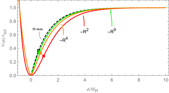
Figure 1: The inflaton potentials of the power-law model (4.1). The Red, Orange, and Green lines show the potential at $n=2$, $4$, $9$. The dashed black line draws the potential of the power-law model with $n\to\infty$. Cross marks($\times$) show the end of inflation, the point at which the slow-roll parameter becomes one, $\epsilon_{V}=1$.

4.2 Logarithmic model

In the context of quantum field theory (QFT), integrating out the heavy degrees of freedom (d.o.f) modifies the potential of the light scalar field. The logarithmic model, which is obtained as

$$f(R)=-\alpha R\ln\Big{(}1+\frac{R}{R_{0}}\Big{)},$$ (4.8)

mimics the one-loop corrections coming from QFT. Importantly, the logarithmic model deforms the corrections to keep the Einstein-Hilbert action at the weak curvature limit. Several variations of the logarithmic corrections have been investigated, as shown in Ref. [40].

In Fig. 2, the inflaton potential of this model has a flat plateau for a large $\phi$ and the quasi-de Sitter expansion is also realized. Thus, we adopt the large field inflation scenario. In other words, the inflaton $\phi$ at the beginning of inflation is larger than the Planck scale. At the limit $\phi\to\infty$ we find from Eq. (2.6),

$$F^{\prime}(R)=0.$$

We can estimate the value of $R$ to solve this equation and the solution is given by

$$R=R_{0}(\frac{1}{W(e^{1-1/\alpha})}-1),$$ (4.9)

where $W(z)$ is the Lambert’s $W$ function. For a small coupling $\alpha<1$, $z=\exp(1-1/\alpha)$ is small enough, $z\ll 1$. The Lauran’s series of $1/W(z)$ around $z=0$ is

$$\frac{1}{W(z)}=\frac{1}{z}+1-\frac{z}{2}+\mathcal{O}(z^{2}),$$ (4.10)

and we obtain $R/R_{0}\sim e^{1/\alpha}\gg 1$. Under this assumption, the function $f(R)$ approaches to the power-law model with $n=1+\alpha$,

$$-\alpha R\ln\Big{(}1+\frac{R}{R_{0}}\Big{)}\sim-\frac{R_{0}}{e}\Big{(}\frac{R}{R_{0}}\Big{)}^{1+\alpha}.$$ (4.11)

The validity of this approximation can be evaluated to compare the inflaton potential of each model in Fig. 3.

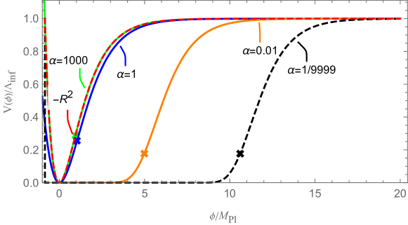
Figure 2: The inflation potential of Eq. (4.8) with $\alpha=0.01$, $1$, and $\alpha=1000$. The dashed Red line is Starobinsky potential from the $R^{2}$ model. The dashed black line is the potential with $\alpha=1/9999$. Cross marks($\times$) show the end of inflation, the point at which the slow-roll parameter becomes one, $\epsilon_{V}=1$.

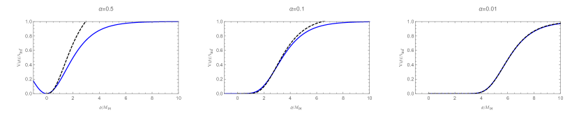
Figure 3: The inflaton potential of Eq. (4.8) is the blue line. The black line represents the potential of the power-law model with $n=1+\alpha$.

For a large coupling, the value of $R/R_{0}$ is less than 1, because Lambert’s $W(z)$ function at $z\sim e$ is almost unity. In this case, the logarithmic model can be approximated to $f(R)=-(\alpha/R_{0})R^{2}$. As the coupling $\alpha$ increases, the potential obtained from Eq. (4.8) approaches that from Eq. (4.1) with $n=2$ (Fig. 2). That is, the $\alpha\to\infty$ limit of the logarithmic model is the Starobinsky model, $f(R)=-R^{2}$.

5 Numerical result

We have analytically evaluated CMB fluctuations for Cartan $F(R)$ gravity in the previous sections. In this section, we numerically calculate the inflationary parameters and show the robustness of the predictions in Cartan $F(R)$ gravity. We perform the numerical calculations in the following steps:

1. $R_{\text{end}}$ is found by the condition for the end of the inflation, $\varepsilon_{V}=1$.

2. $R_{*}$ is obtained from Eq. (3.4) with the e-folding number, $N=50,60$.

3. The CMB fluctuations, $n_{s}$ (3.6), $\alpha_{s}$ (3.7) and $r$ (3.8) are estimated from the slow-roll parameters, $\varepsilon_{V}$ (3.1), $\eta_{V}$ (3.2), $\xi_{V}$ (3.3) at $R*$.

First, we consider the power-law model of Eq. (4.1). The potential of the power-law model can be expressed as

$$V(\phi)\propto\left(1-e^{-\sqrt{\frac{2}{3}}\frac{\phi}{{M_{\rm Pl}}}}\right)^{1+\frac{1}{n-1}}.$$ (5.1)

At the limit $n\to\infty$, the potential becomes

$$\left.V(\phi)\right|_{n\to\infty}\propto 1-e^{-\sqrt{\frac{2}{3}}\frac{\phi}{{M_{\rm Pl}}}}.$$ (5.2)

Starting from this potential, we can calculate the CMB fluctuations. Figure 4 shows the numerical results for the power-law model with $n=2-9$ and $\infty$. In these figures, the attractor points at $n\to\infty$ are shown by the red diamonds. It is remarkable that the results are consistent with the observation even at the limit, $n\to\infty$. The predicted spectrum indices have a narrow range of variation of about $10^{-3}$ for a change of $n=2$ to $\infty$ in the parameters of the power-law model.

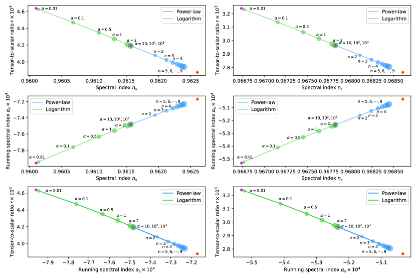
Figure 4: Numerical results of CMB fluctuations, $n_{s}-r$ (Top), $\alpha_{s}-r$ (Middle), and $n_{s}-\alpha_{s}$ (Bottom) at $N=50$ (Left) and $N=60$ (Right). The Blue lines represent the power-law model with $n=2-9$ and the Green lines are the logarithmic model with $\alpha=0.01,0.1,0.5,1,2,10,100,1000$. The red and magenta diamonds show the attractor points at $\alpha=1/9999$, $\alpha\to\infty$, and $n\to\infty$.

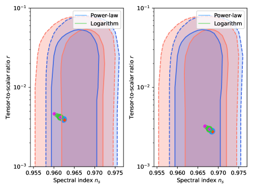
Figure 5: Numerical result of CMB fluctuations, $n_{s}-r$ for the power-law and logarithmic models at $N=50$ (Left) and $N=60$ (Right) with Planck constraints. The blue and red area shows the Planck 2018 constraints in [37].

Next, we analyze the logarithmic model (4.8) and show the results in Fig. 4. We observe that the CMB fluctuations in the logarithmic model approach to those in the $R^{2}$ model as $\alpha$ increases. As explained at the end of the previous section, this model is close to the Starobinsky model at the limit, $\alpha\to\infty$. Thus, we can understand why the fluctuations approach those of the $R^{2}$ model as $\alpha$ increases.

For small coupling, this model is approximated as $f(R)\sim R^{1+\alpha}$ from Eq. (4.11). Consequently, the logarithmic model with small coupling can be rewritten by the power-law model with $n=1+\alpha$. From Eq. (5.1) the potential is given by

$$V(\phi)\propto\left(1-e^{-\sqrt{\frac{2}{3}}\frac{\phi}{{M_{\rm Pl}}}}\right)^{1+\frac{1}{\alpha}}.$$ (5.3)

It should be noted that the slow-roll scenario can not be adapted because of the vanishing potential energy at the limit, $\alpha\to 0$. However, as can be seen in Fig. 4, even at extreme values such as $\alpha=1/9999$, the CMB fluctuations do not vary significantly and show attractor-like behavior.

Next we summarize the numerical results of the power-law and logarithmic models in Figure 5 and Table 1. From Fig. 5, the numerical results of the entire parameter region for Cartan $F(R)$ gravity satisfies the constraints of Planck 2018 [37]. In other words, all the results are consistent with the current observations. In these models the variation in CMB fluctuations is within a narrow range. These results demonstrate the robustness of certain Cartan $F(R)$ gravity models.

Model	Parameter	$N$	$n_{s}$	$\alpha_{s}$	$r$
Power-law(4.1)	$n=2$	50	0.9616	-0.000748	0.00419
		60	0.9678	-0.000523	0.00296
	$n=9$	50	0.9624	-0.000723	0.00394
		60	0.9685	-0.000507	0.00280
	$n\to\infty$	50	0.9626	-0.000717	0.00388
		60	0.9686	-0.000503	0.00276
Logarithmic(4.8)	$\alpha=1/9999$	50	0.9601	-0.000796	0.00464
		60	0.9667	-0.000553	0.00324
	$\alpha=0.01$	50	0.9601	-0.000796	0.00464
		60	0.9667	-0.000553	0.00324
	$\alpha=1000$	50	0.9616	-0.000748	0.00419
		60	0.9678	-0.000523	0.00296
	$\alpha\to\infty$	50	0.9616	-0.000748	0.00419
		60	0.9678	-0.000523	0.00296
Constraints [37]	-	-	$0.967\pm 0.004$	$-0.0042\pm 0.0067$	$<0.065$

Table 1: Numerical results of spectral index ($n_{s}$), running spectral index ($\alpha_{s}$), tensor-to-scalar ratio ($r$) in power-law and Logarithmic models at e-folding number $N=50,60$.

6 Reheating

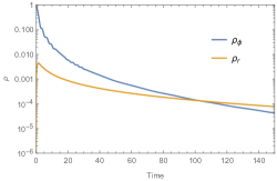
(a) Power-law model($n=2$)

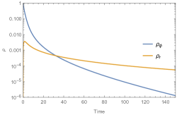
(b) Logarithmic model($\alpha=0.01$)

Figure 6: Numerical results of the time evolution of energy densities. Time is scaled by $\tilde{t}=Mt$ and $\Gamma/M=10^{-2}$ where $M=10^{15}$GeV. The initial time is specified at the end of inflation, $\epsilon_{V}=1$.

When considering a realistic cosmological scenario, it is essential to incorporate reheating processes after inflation. During the reheating process, the energy of the inflaton transitions to radiation and the universe enters a radiation-dominated era. In this section, we consider the reheating process in Cartan $F(R)$ gravity.

We perform numerical calculations of the reheating process for $n=2$ in the power-law model and $\alpha=0.01$ in the logarithmic model. Let us assume that the decay rate from inflaton to radiation is $\Gamma$. The equation of motion for the inflaton becomes

$$\ddot{\phi}+3H\dot{\phi}+V^{\prime}(\phi)=-\Gamma\dot{\phi}.$$ (6.1)

Next, the equation for the energy density of radiation is given as

$$\dot{\rho}_{r}+4H\rho_{r}=\Gamma\rho_{r}.$$ (6.2)

Also, Friedmann equation is

$$3H^{2}{M_{\rm Pl}}^{2}=\rho_{\phi}+\rho_{r},$$ (6.3)

where $\rho_{\phi}$ is the energy density of inflaton $\phi$;

$$\rho_{\phi}=\frac{1}{2}\dot{\phi}^{2}+V(\phi).$$

From Eqs. (6.1), (6.2), and (6.3), the time evolution of the energy densities is calculated numerically. These results are in Fig. 6. In addition, Table. 2 shows the starting time of the radiation-dominated era $\tilde{t}_{R}$ and the reheating temperature $T_{R}$. The numerical reheating temperatures are in order agreement with analytical results [41]. We have demonstrated that the reheating process occurs in each model of Cartan $F(R)$ gravity.

For other model parameters, the logarithmic model with a large coupling approximates the $R^{2}$ model with the Starobinsky potential. In the power-law model with $n>2$, the potential can be approximated as $|\phi|^{1+\frac{1}{n-1}}$ around $\phi=0$ when $n$ is even. Although there may be a slight difference in the oscillation at the bottom of the potential, a similar reheating process can be considered. On the other hand, when $n$ is odd, a region where $\phi<0$ cannot be defined, and instant reheating or preheating is required [42, 43].

In this study, we assume a constant friction term, $\Gamma$. As a future development, we aim to consider the friction term through interactions obtained from Cartan formalism.

Model	$\tilde{t}_{R}$	$T_{R}$[GeV]
Power-law($n=2$)	103	$5.4\times 10^{10}$
Logarithmic($\alpha=0.01$)	32.2	$7.4\times 10^{10}$

Table 2: Numerical results of reheating in power-law and Logarithmic models.

7 Conclusion

We have studied Cartan $F(R)$ gravity, an extension of $F(R)$ gravity on Riemann-Cartan geometry. We constructed a derivation of the scalar-tensor theory from Cartan $F(R)$ gravity. A scalar field with a canonical kinetic term is introduced by extracting the torsion from the curvature scalar. The potential term is derived from the modified gravity action, $f(R)$. Since the derivation does not require a conformal transformation, it is free from the equivalence problem between Jordan and Einstein frames in conventional $F(R)$ gravity.

The derived scalar-tensor theory has been applied to the slow-roll scenario of inflation. We have developed the formulations in Eqs. (3.1)-(3.3) and (3.4) for the CMB fluctuations in Cartan $F(R)$ gravity. In these formulations, it is possible to compute the results directly from the $F(R)$ form without expressing the potential in terms of a scalar field. The CMB fluctuations have been calculated for the power-law and logarithmic models. We have found that the obtained results are consistent with observations and concluded that Cartan $F(R)$ gravity gives a realistic inflation model. We have also shown that the CMB fluctuations are robust to variations in the model parameters. Additionally, this means that Cartan $F(R)$ gravity is also valid when a low-energy effective theory of quantum gravity is assumed to present a polynomial form. These results in the power-law model differ from the conventional $F(R)$ gravity where the potential has a local maximum if the exponent is larger than two ($n>2$) and fine-tuning is unavoidable to have a realistic e-folding number [39].

It is interesting to investigate whether the robustness of Cartan $F(R)$ gravity is a generic feature. We would like to apply the model for the reheating process after inflation [44, 45, 46, 47]. The reheating process may also reveal different features from the conventional $F(R)$ gravity. The original ECKS theory has a four-fermion interaction called spin-spin interaction or Dirac-Heisenberg-Ivanenko-Hehl-Datta four-body fermi interaction [48, 49, 50, 51, 52]. Cartan $F(R)$ gravity has been associated with matter fields such as spin-spin interaction through torsion. The interaction between the inflaton and matter fields produces a reheating process. It then reveals the growth of the universe leading to standard cosmology.

Appendix A Lambert’s function

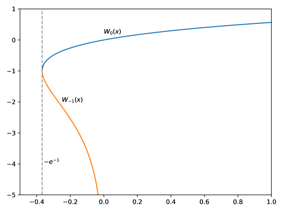
Figure 7: Two branches of the Lambert’s $W$ function. The blue line, $W_{0}$, is the principal branch which is defined the interval $(-e^{{}^{1}},\infty)$ and the red line, $W_{-1}$, is other branch in the interval $(-e^{-1},0)$. The branching point is at $(-e^{-1},-1)$.

In this section, we briefly introduce Lambert’s $W$ function. For more details see Ref. [53] as an example. The function $W(x)$ is defined to satisfy the following equation

$$W(x)e^{W(x)}=x,$$ (A.1)

where $W(x)$ is called the Lambert’s $W$ function. The $W$ function has two branches. One is defined in the interval $[-e^{-1},\infty]$, and other is in the interval $(-e^{-1},0)$. The former is called the principal branch and described as $W_{0}$, while the latter is written as $W_{-1}$. The branching point is at $(-e^{-1},-1)$. See, fig. 7.

For $x>0$, the principal branch can rearrange eq. (A.1) to take the natural log,

$$W(x)=\ln x-\ln W(x),$$ (A.2)

then we can obtain the recursive relation,

$$W_{0}(x)=\ln x-\ln(\ln x-\ln(\ln x-\cdots)),$$ (A.3)

and, for $x<0$, we can obtain the similar relation for $W_{-1}$ as

$$W_{-1}(x)=\ln(-x)-\ln(-(\ln(-x)-\ln(-\ln(-x+\cdots)))).$$ (A.4)

The asymptotic expansion of Lambert function is estimated by using Lagrange inverse theorem as

$$W(x)= L_{1}-L_{2}+\frac{L_{2}}{L_{1}}+\frac{L_{2}(-2+L_{2})}{2L_{1}^{2}}+\frac{L_{2}(6-9L_{2}+2L_{2}^{2})}{6L_{1}^{3}}$$

$$+\frac{L_{2}(-12+36L_{2}-22L_{2}^{2}+3L_{2}^{3})}{12L_{1}^{4}}+\mathcal{O}\Big{(}\big{\{}\frac{L_{2}}{L_{1}}\big{\}}^{5}\Big{)},$$ (A.5)

where $L_{1}=\ln x$ and $L_{2}=\ln\ln x$ for the principle branch, and $L_{1}=\ln(-x)$ and $L_{2}=\ln(-\ln(-x))$ for the negative branch. Note that the expansion (A.5) is convergent at both 0 and infinity. See [54] for details.

Appendix B Exact solution of Starobinsky model in Riemann geometry

As the power-law model of Cartan $F(R)$ gravity, the inflationary observables of the Starobinsky model in Riemann geometry can be represented analytically.

The e-folding number of Starobinsky model is expressed by

$$N=\frac{3}{4}\Big{(}2\gamma R-\ln(1+2\gamma R)\Big{)}\Big{|}_{R_{\text{end}}}^{R_{*}},$$ (B.1)

and the curvature $R_{*}$ is solved as

$$R_{*}=-1-W_{-1}\Big{(}-e^{-\big{(}1+4N/3\big{)}}\Big{)}.$$ (B.2)

$$n_{s}=1+\frac{8}{3}\frac{1}{1+W_{-1}(-e^{-(1+4N/3)})}-\frac{16}{3}\Big{(}\frac{1}{1+W_{-1}(-e^{-(1+4N/3)})}\Big{)}^{2}\sim 1-\frac{2}{N}-\frac{3}{N^{2}},$$ (B.3)

$$r=\frac{64}{3}\Big{(}\frac{1}{1+W_{-1}(-e^{-(1+4N/3)})}\Big{)}^{2}\sim\frac{12}{N^{2}},$$ (B.4)

$$\begin{aligned} \alpha_{s}=&-\frac{32}{9}\Big{(}\frac{1}{1+W_{-1}(-e^{-(1+4N/3)})}\Big{)}^{2}+\frac{160}{9}\Big{(}\frac{1}{1+W_{-1}(-e^{-(1+4N/3)})}\Big{)}^{3}\\ &-\frac{128}{3}\Big{(}\frac{1}{1+W_{-1}(-e^{-(1+4N/3)})}\Big{)}^{4}\\ \sim&-\frac{2}{N^{2}}-\frac{15}{2N^{3}}-\frac{27}{2N^{4}}.\end{aligned}$$ (B.5)

The approximation of r.h.s of eqs. (B.3), (B.4), (B.5) are evaluated to apply the recursive formula (A.4).

References

- [1] B.A. Bassett, S. Tsujikawa and D. Wands, Inflation dynamics and reheating, Rev. Mod. Phys. 78 (2006) 537 [astro-ph/0507632].
- [2] D.C. Maurya, Accelerating scenarios of massive universe in f(R,Lm)-gravity, New Astron. 100 (2023) 101974.
- [3] J.R.L. Santos and R.S. Santos, Cosmological models in gravity, 2303.16714.
- [4] S. Taghavi, K. Saaidi, Z. Ossoulian and T. Golanbari, Holographic inflation in gravity and observational constraints, 2301.02631.
- [5] A.A. Starobinsky, Spectrum of relict gravitational radiation and the early state of the universe, JETP Lett. 30 (1979) 682.
- [6] A.A. Starobinsky, A New Type of Isotropic Cosmological Models Without Singularity, Phys. Lett. B 91 (1980) 99.
- [7] K. Sato, First Order Phase Transition of a Vacuum and Expansion of the Universe, Mon. Not. Roy. Astron. Soc. 195 (1981) 467.
- [8] A.H. Guth, The Inflationary Universe: A Possible Solution to the Horizon and Flatness Problems, Adv. Ser. Astrophys. Cosmol. 3 (1987) 139.
- [9] S. Nojiri and S.D. Odintsov, Introduction to modified gravity and gravitational alternative for dark energy, eConf C0602061 (2006) 06 [hep-th/0601213].
- [10] S. Nojiri and S.D. Odintsov, Unified cosmic history in modified gravity: from F(R) theory to Lorentz non-invariant models, Phys. Rept. 505 (2011) 59 [1011.0544].
- [11] S. Nojiri, S. Odintsov and V. Oikonomou, Modified Gravity Theories on a Nutshell: Inflation, Bounce and Late-time Evolution, Phys. Rept. 692 (2017) 1 [1705.11098].
- [12] P. Jordan and E. Schücking, Schwerkraft und Weltall: Grundlagen der theoretischen Kosmologie, Die Wissenschaft, F. Vieweg (1955).
- [13] R. Catena, M. Pietroni and L. Scarabello, Einstein and Jordan reconciled: a frame-invariant approach to scalar-tensor cosmology, Phys. Rev. D 76 (2007) 084039 [astro-ph/0604492].
- [14] C.F. Steinwachs and A.Y. Kamenshchik, One-loop divergences for gravity non-minimally coupled to a multiplet of scalar fields: calculation in the Jordan frame. I. The main results, Phys. Rev. D 84 (2011) 024026 [1101.5047].
- [15] A.Y. Kamenshchik and C.F. Steinwachs, Question of quantum equivalence between Jordan frame and Einstein frame, Phys. Rev. D 91 (2015) 084033 [1408.5769].
- [16] Y. Hamada, H. Kawai, Y. Nakanishi and K.-y. Oda, Meaning of the field dependence of the renormalization scale in Higgs inflation, Phys. Rev. D 95 (2017) 103524 [1610.05885].
- [17] T. Inagaki and M. Taniguchi, Cartan F(R) Gravity and Equivalent Scalar–Tensor Theory, Symmetry 14 (2022) 1830 [2204.01255].
- [18] D.W. SCIAMA, The physical structure of general relativity, Rev. Mod. Phys. 36 (1964) 463.
- [19] T.W.B. Kibble, Lorentz invariance and the gravitational field, Journal of Mathematical Physics 2 (1961) 212 [https://doi.org/10.1063/1.1703702].
- [20] C.G. Boehmer and J. Burnett, Dark spinors with torsion in cosmology, Phys. Rev. D 78 (2008) 104001 [0809.0469].
- [21] N.J. Popławski, Cosmology with torsion: An alternative to cosmic inflation, Phys. Lett. B 694 (2010) 181 [1007.0587].
- [22] J.a. Magueijo, T.G. Zlosnik and T.W.B. Kibble, Cosmology with a spin, Phys. Rev. D 87 (2013) 063504 [1212.0585].
- [23] M. Shaposhnikov, A. Shkerin, I. Timiryasov and S. Zell, Einstein-Cartan gravity, matter, and scale-invariant generalization , JHEP 10 (2020) 177 [2007.16158].
- [24] M. Shaposhnikov, A. Shkerin, I. Timiryasov and S. Zell, Higgs inflation in Einstein-Cartan gravity, JCAP 02 (2021) 008 [2007.14978].
- [25] D. Iosifidis and L. Ravera, The cosmology of quadratic torsionful gravity, Eur. Phys. J. C 81 (2021) 736 [2101.10339].
- [26] F. Cabral, F.S.N. Lobo and D. Rubiera-Garcia, Imprints from a Riemann–Cartan space-time on the energy levels of Dirac spinors, Class. Quant. Grav. 38 (2021) 195008 [2102.02048].
- [27] M. Piani and J. Rubio, Higgs-Dilaton inflation in Einstein-Cartan gravity, JCAP 05 (2022) 009 [2202.04665].
- [28] M. Montesinos, R. Romero and D. Gonzalez, The gauge symmetries of gravity with torsion in the Cartan formalism, Class. Quant. Grav. 37 (2020) 045008 [2001.08759].
- [29] T.P. Sotiriou and S. Liberati, The Metric-affine formalism of f(R) gravity, J. Phys. Conf. Ser. 68 (2007) 012022 [gr-qc/0611040].
- [30] T.P. Sotiriou and S. Liberati, Metric-affine f(R) theories of gravity, Annals Phys. 322 (2007) 935 [gr-qc/0604006].
- [31] D. Iosifidis, A.C. Petkou and C.G. Tsagas, Torsion/non-metricity duality in f(R) gravity, Gen. Rel. Grav. 51 (2019) 66 [1810.06602].
- [32] S. Capozziello, R. Cianci, C. Stornaiolo and S. Vignolo, f(R) gravity with torsion: The Metric-affine approach, Class. Quant. Grav. 24 (2007) 6417 [0708.3038].
- [33] S. Capozziello, R. Cianci, C. Stornaiolo and S. Vignolo, f(R) gravity with torsion: A Geometric approach within the J-bundles framework, Int. J. Geom. Meth. Mod. Phys. 5 (2008) 765 [0801.0445].
- [34] T.P. Sotiriou, f(R) gravity, torsion and non-metricity, Class. Quant. Grav. 26 (2009) 152001 [0904.2774].
- [35] S. Capozziello and S. Vignolo, Metric-affine f(R)-gravity with torsion: An Overview, Annalen Phys. 19 (2010) 238 [0910.5230].
- [36] G.J. Olmo, Palatini Approach to Modified Gravity: f(R) Theories and Beyond, Int. J. Mod. Phys. D 20 (2011) 413 [1101.3864].
- [37] Planck collaboration, Planck 2018 results. X. Constraints on inflation, Astron. Astrophys. 641 (2020) A10 [1807.06211].
- [38] H. Motohashi, Consistency relation for inflation, Phys. Rev. D 91 (2015) 064016 [1411.2972].
- [39] T. Inagaki and H. Sakamoto, Exploring the inflation of gravity, Int. J. Mod. Phys. D 29 (2020) 2050012 [1909.07638].
- [40] S. Nojiri and S.D. Odintsov, Modified gravity with ln R terms and cosmic acceleration, Gen. Rel. Grav. 36 (2004) 1765 [hep-th/0308176].
- [41] K.D. Lozanov, Lectures on Reheating after Inflation, 1907.04402.
- [42] G.N. Felder, L. Kofman and A.D. Linde, Instant preheating, Phys. Rev. D 59 (1999) 123523 [hep-ph/9812289].
- [43] J. de Haro, Reheating constraints in instant preheating, Phys. Rev. D 107 (2023) 123511 [2304.05903].
- [44] A. Nishizawa and H. Motohashi, Constraint on reheating after inflation from gravitational waves, Phys. Rev. D 89 (2014) 063541 [1401.1023].
- [45] V.K. Oikonomou, Reheating in Constant-roll Gravity, Mod. Phys. Lett. A 32 (2017) 1750172 [1706.00507].
- [46] A. Mathew and M.K. Nandy, Primordial reheating in cosmology by spontaneous decay of scalarons, 2012.13960.
- [47] F. Rajabi and K. Nozari, Reheating and particle creation in unimodular f(R, T) gravity, Eur. Phys. J. C 82 (2022) 995 [2211.00594].
- [48] F. Hehl, G. Kerlick and P. Von Der Heyde, General relativity with spin and torsion and its deviations from einstein’s theory, Phys. Rev. D 10 (1974) 1066.
- [49] G. Kerlick, Cosmology and Particle Pair Production via Gravitational Spin Spin Interaction in the Einstein-Cartan-Sciama-Kibble Theory of Gravity, Phys. Rev. D 12 (1975) 3004.
- [50] M. Gasperini, Spin Dominated Inflation in the Einstein-cartan Theory, Phys. Rev. Lett. 56 (1986) 2873.
- [51] F. Hehl and B. Datta, Nonlinear spinor equation and asymmetric connection in general relativity, J. Math. Phys. 12 (1971) 1334.
- [52] J. Boos and F.W. Hehl, Gravity-induced four-fermion contact interaction implies gravitational intermediate W and Z type gauge bosons, Int. J. Theor. Phys. 56 (2017) 751 [1606.09273].
- [53] D. Veberic, Having fun with lambert w(x) function, CoRR abs/1003.1628 (2010) [1003.1628].
- [54] R.M. Corless, G.H. Gonnet, D.E.G. Hare, D.J. Jeffrey and D.E. Knuth, On the lambertw function, Advances in Computational Mathematics 5 (1996) 329.