Shadows and quasinormal modes of the Bardeen black hole in cloud of strings

Abstract

We investigate the black hole (BH) solution of the Einstein’s gravity coupled with non-linear electrodynamics (NED) source in the background of a cloud of strings. We analyze the horizon structure of the obtained BH solution. The optical features of the BH are explored. The photon radius and shadows of the BH are obtained as a function of black hole parameters. We observe that the size of the shadow image is bigger than its horizon radius and photon sphere. We also study the Quasinormal modes (QNM) using WKB formula for this black hole. The dependence of shadow radius and QN modes on black hole parameters reflects that they are mimicker to each other.

I Introduction

The black holes are singular solutions of the general theory of relativity (GTR). The singularity is masked by the presence of the black hole (BH) horizon (Cosmic Censorship hypothesis). However, the singularity can be avoided in higher derivative theories of gravity itself or by coupling GTR with higher derivative matter theories 8 and this can be a plausible mechanism by which nature can avoid space-time singularities 1a . Several black hole solutions of higher derivative theories exist in literature when gravity is coupled with suitable nonlinear electrodynamics (NED) source e.g. Born-Infeld charged black hole (BH) Jafarzade:2020ova , Culetu BH in the presence of cosmic string Singh:2022ycn , regular Einstein Gauss-Bonnet (EGB) black holes Singh:2022dth , charged $AdS$ Belhaj:2020nqy and charged $AdS$ EGB black hole EslamPanah:2020hoj . Bardeen black hole happens to be a regular solution and it can be obtained as a charged solution of GTR coupled with NED abg11 ; abg . In fact, it is a magnetically charged solution resulting from a self-gravitating monopole. There exist many other BH solutions based on the Bardeen model bar ; fr1 ; Singh:2017qur ; bambi ; Ahmed:2022qge ; sh11 ; Singh:2017bwj ; rizzo06 ; Ghosh:2020tgy ; Ghosh:2020ijh ; Singh:2020nwo ; Singh:2019wpu ; Singh:2020rnm ; Singh:2021nvm ; Maluf:2018lyu ; ma14 ; dvs19 ; sabir ; Bronnikov:2000vy ; Simpson:2019mud ; Panotopoulos:2019qjk ; Singh:2022xgi ; Singh:2020xju ; bhu .

Investigation of particle motion in black hole space-time and shadows thereof provides an interesting laboratory to test Einstein’s General theory of relativity. The shadow size depends on black hole mass and parameters like charge and angular momentum. At the same time, black holes have characteristic oscillation frequencies known as Quasi-normal modes (QNM), and these modes are dependent on black hole parameters. The dependence seems to have a direct correspondence with the dependence of shadow radius and QNM Tsukamoto:2014tja ; Li:2021zct ; Cuadros-Melgar:2020kqn ; moura2021 with BH parameters. These features are investigated recently for several types of BH’s with asymptotic flat or $AdS$ space-time Sakharov:1966 ; Gliner:1966 .

In this paper, we consider a BH space-time that is neither flat nor $AdS$ asymptotically. An example of this kind of space-time can be obtained by considering of BH solution in a cloud of cosmic strings Rodrigues:2022zph ; Rodrigues:2022rfj . Motivated by the recent astrophysical observations akima19 ; akima2019 , we are interested in the optical features of the Bardeen BH’s in the presence of cosmic string. This solution becomes the Letelier solution xu19 ; l1 ; l2 in a certain limit. The cosmic strings and magnetic monopoles may have been produced amply in the early universe and it makes sense to think of Bardeen BH immersed in a cloud of strings. This kind of background is not asymptotically flat but provides a consistent gravitational solution.

Here, we consider the Bardeen BH solution in a cloud of strings (CoS) and study the shadows and QNM produced by it. We review the BH solution with CoS parameter using the NED in Sec. II and study its horizon structure. In sec. III we study the BH shadows and QNM. We summarise and discuss our results in Sec. IV.

II Exact solution of Bardeen black hole in a cloud of string

The solution of Bardeen black hole solution in CoS was obtained by Rodrigues et. al Rodrigues:2022zph ; Rodrigues:2022rfj and we outline the procedure here. Let us begin with a theory of gravity in the presence of NED source and CoS parameters. The action is given by,

$$S=\int d^{4}x\sqrt{-g}\left[R+{\cal L}_{NED}+{\cal L}_{cs}\right],$$ (1)

where $g$ is the metric determinant and $R$ denotes the Ricci scalar. The action terms of NED and CoS are specified below. The equations of motion (EoM) can be obtained by the variation of the action (1) with respect to $g_{\mu\nu}$ and $A_{\mu}$,

$$R_{ab}-\frac{1}{2}\tilde{g}_{ab}R=^{NED}T_{\mu\nu}+^{CS}T_{\mu\nu}$$ (2)

$$\nabla_{a}\left(\frac{\partial{{L(F)}}}{\partial F}F^{ab}\right)=0\qquad\text{and}\qquad\nabla_{a}(*F^{ab})=0,$$ (3)

where $L(F)$ denotes the Lagrangian density of NED, taken as a function of $F=F_{\mu\nu}F^{\mu\nu})$. The source of the NED (Bardeen type) is Singh:2020xju ; Singh:2017qur

$${{L(F)}}=\frac{3}{2sg^{2}}\left(\frac{\sqrt{2g^{2}F}}{1+\sqrt{2g^{2}F}}\right)^{\frac{5}{2}}$$ (4)

where $s=g/2M$, where $M$ and $g$ are the free parameters associated with magnetic monopole charge and mass. The matter energy-momentum tensor (EMT) can also be obtained from the Eq. (4) and is given by,

$$T_{\mu\nu}^{NED}=2\left[\frac{\partial{{L(F)}}}{\partial F}F_{\mu\sigma}F_{\nu}^{\sigma}-\tilde{g}_{\mu\nu}{{L(F)}}\right],$$ (5)

The nonvanishing components of EMT are

$${T}^{t}_{t}={T}^{r}_{r}=\frac{8Mg^{2}}{(r^{2}+g^{2})^{5/2}}$$ (6)

$$T^{\theta}_{\theta}=T^{\phi}_{\phi}=\frac{8Mg^{2}(r^{2}-4)}{(r^{2}+g^{2})^{5/2}}$$ (7)

Let us consider the CoS as a source governed by the Nambu-Goto action and is given by xu19

$$S_{\text{NG}}=\int_{\Sigma}\;m(-\gamma)^{-1/2}d\lambda^{0}d\lambda^{1}=\int_{\Sigma}\;m\left(-\frac{1}{2}\Sigma^{\mu\nu}\Sigma_{\mu\nu}\right)^{1/2}d\lambda^{0}d\lambda^{1},$$ (8)

where $\gamma$ is the determinant of the reduced metric and $m$ is a constant characterizes the mass of the each string. $\lambda^{0}$ and $\lambda^{1}$ are local time-like and space-like coordinates respectively 24 . The $\Sigma^{\mu\nu}$ is a bivector which is written as

$$\Sigma^{\mu\nu}=\epsilon^{ab}\frac{\partial x^{\mu}}{\partial\lambda^{a}}\frac{\partial x^{\nu}}{\partial\lambda^{b}},$$ (9)

where $\epsilon^{ab}$ is the Levi-Civta tensor which takes the following non-zero values: $\epsilon^{01}=-\epsilon^{10}=1$. Using the definition, the EMT for CoS is given by xu19 ; Singh:2020nwo ; Singh:2022ycn

$$T^{\mu\nu}=\frac{\rho\Sigma^{\mu\rho}\Sigma_{\rho}^{\phantom{\rho}\nu}}{\sqrt{-\gamma}}.$$ (10)

where $\rho$ is the density. The nonvanishing components of the CoS are

$$T^{t}_{t}=T^{r}_{r}=\frac{a}{r^{2}},$$ (11)

$$T^{\theta}_{\theta}=T^{\phi}_{\phi}=\frac{a}{r^{2}},$$ (12)

where $a$ is a constant known as CoS parameter.

In order to find the BH solution coupled with the CoS and NED source, one can consider the static spherically symmetric space-time, which is described by the following line element

$$ds^{2}=-f(r)dt^{2}+\frac{1}{f(r)}dr^{2}+r^{2}d\Omega^{2},$$ (13)

with

$$f(r)=1-\frac{2m(r)}{r},$$ (14)

where $d\Omega^{2}=d\theta^{2}+\sin^{2}\theta d\phi^{2}$. Inserting the Eqs. (11), (12), and (13) in Eq. (2), the Einstein field equations become

$$\frac{d}{dr}m(r)=\frac{2Mg^{2}}{(r^{2}+g^{2})^{5/2}}+\frac{a}{2}.$$ (15)

Integrating the Eq. (15) with respect to $r$. The (15) becomes

$$m(r)=\frac{Mr^{3}}{(r^{2}+g^{2})^{3/2}}+\frac{a}{2}r+C_{1},$$ (16)

where $C_{1}$ is constant to be identified with black hole mass, M. The line element of the black hole metric is obtained as Rodrigues:2022zph ; Rodrigues:2022rfj ,

$$ds^{2}=-\left(1-\frac{2Mr^{2}}{(r^{2}+g^{2})^{3/2}}-a\right)dt^{2}+\frac{dr^{2}}{\left(1-\frac{2Mr^{2}}{(r^{2}+g^{2})^{3/2}}-a\right)}+r^{2}d\Omega_{2}^{2}.$$ (17)

The solution (17) is characterized by magnetic charge, $g$, and CoS parameter, $a$. The solution is exact and provides a new example in the presence of NED and CoS. In the limit, $g=0$, the resulting solution reduces to the Letelier solution xu19 and it becomes Bardeen solution Singh:2017qur in the absence of CoS source. It (17) coincides with the Schwarzschild BH solution for $g=0$ and $a=0$.

Now, we study the nature of the BH horizon for the obtained BH solution (17) when $(f(r)=0$:

$$1-\frac{2Mr^{2}}{(r^{2}+g^{2})^{3/2}}-a=0$$ (18)

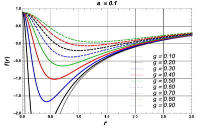
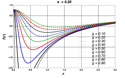
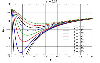
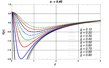
Figure 1: Metric function $f(r)$ versus $r$ for values of magnetic charge $g$ and $a=0.1\,,0.2\,\,0.3$ etc. for fixed values of $M$ and $l$.

The analytic solution of Eq. (18) does not exist and we solve it numerically in Fig.(1). The numerical values of the horizon radii are shown in table (1) for different values of the CoS parameter, $a$, and magnetic charge, $g$. In Tab. (1), we see that the size of the BH horizon decreases with growing magnetic charge, $g$, and CoS parameter, $a$. The BH solution has degenerated at the value of $(g_{c}=0.85)$ and $(a=0.1)$ the BH horizon merges are known as the degenerate horizon. When the value of $g>0.85$, no black hole solutions exists. The critical value $g_{c}$ also increases with the increase in the CoS parameter, $a$.

		$a=0.1$			$a=0.2$			$a=0.3$
$g$	$r_{-}$	$r_{+}$	$\delta$	$r_{-}$	$r_{+}$	$\delta$	$r_{-}$	$r_{+}$	$\delta$
0.1	0.020	2.24	2.22	0.0207	2.51	2.489	0.0276	2.87	2.842
0.2	0.0622	2.19	2.12	0.0737	2.47	2.396	0.0753	2.84	2.764
0.3	0.131	2.17	2.04	0.110	2.44	2.330	0.110	2.82	2.710
0.4	0.207	2.11	1.903	0.193	2.41	2.217	0.165	2.76	2.595
0.5	0.297	2.03	1.733	0.285	2.35	2.065	0.237	2.73	2.493
0.6	0.421	1.94	1.519	0.359	2.26	1.901	0.331	2.66	2.329
0.7	0.581	1.80	1.219	0.506	2.12	1.614	0.451	2.57	2.119
0.8	0.829	1.61	0.781	0.672	2.02	1.348	0.571	2.46	1.889
$g_{c}$	1.197	1.197	0	1.327	1.327	0	1.521	1.521	0

Table 1: The analysis of inner and outer horizon for different values of CoS parameter, $a$ and magnetic charge, $g$ for a fixed value of $M=1$. The critical value of magnetic charge is $g_{c}=0.85\,,0.97$ and $1.12$ corresponding to the $a=0.1\,,0.2$ and $0.3$ respectively.

It was shown by Rodriques et. al. Rodrigues:2022zph ; Rodrigues:2022rfj that the curvature invariants like Kretschmann scalar $R_{\mu\nu\lambda\sigma}R^{\mu\nu\lambda\sigma}$ remain singular at the center for non-zero value of CoS parameter, a. This is unlike the Bardeen solution where the singularity at the center was resolved by magnetic charge.

III Shadow and Quasi normal Modes

Let us consider the massless photon moving in the background of the BH solution (17). We consider the motion of the photon restricted to the equatorial plane by demanding $\theta=\pi/2$. The corresponding EoM can be obtained using the Hamiltonian Belhaj:2020okh ; Belhaj:2022kek ; Belhaj:2021tfc ,

$$H=\frac{1}{2}\left[-\frac{p_{t}^{2}}{f(r)}+f(r)p_{r}^{2}+\frac{p_{\phi}^{2}}{r^{2}}\right].$$ (19)

The canonically conjugate momentum for the BH metric (17) can be obtained as

$$p_{t}=\left(1-\frac{2Mr^{2}}{(r^{2}+g^{2}){3/2}}-a\right){\dot{t}}=E,\qquad\qquad p_{r}=\left[\left(1-\frac{2Mr^{2}}{(r^{2}+g^{2}){3/2}}-a\right)\right]^{-1}{\dot{r}},$$

$$p_{\theta}=r^{2}{\dot{\theta}},\qquad\qquad\qquad\quad\quad\qquad\qquad\qquad\qquad p_{\phi}=r^{2}\sin^{2}\theta{\dot{\phi}}=L.$$ (20)

where $E$ and $L$ are the energy and angular momentum respectively. The EoM is obtained as

$${\dot{t}}=\frac{E}{\left(1-\frac{2Mr^{2}}{(r^{2}+g^{2}){3/2}}-a\right)},\qquad\qquad r^{2}{\dot{r}}=\pm\sqrt{\cal R}$$

$$r^{2}{\dot{\theta}}=\pm\sqrt{{\Theta}},\qquad\qquad\qquad\qquad\quad{\dot{\phi}}=\frac{L}{r^{2}}.$$ (21)

We can re-write the radial null geodesics equation as follows

$${\dot{r}}^{2}+V_{eff}(r)=0\qquad\text{with}\qquad V_{eff}=f(r)\left(\frac{L^{2}}{r^{2}}+\frac{E^{2}}{f(r)}\right)$$ (22)

The null circular geodesics satisfies the following conditions

$$V_{eff}=0,\qquad\text{and}\qquad\frac{\partial V_{eff}}{\partial r}=0.$$ (23)

and it gives

$$\frac{(1-a)(g^{2}+r^{2}_{p})^{5/2}-3Mr^{4}_{p}}{(g^{2}+r^{2}_{p})[(1-a)(g^{2}+r^{2}_{p})^{5/2}-2Mr^{2}_{p}]}=0.$$ (24)

The analytic solution can not be obtained for the photon radius from this equation. The numerical values radius of photon for different values of magnetic charge, $g$, and CoS parameter, $a$ and are listed below:

					$r_{p}$
$a$	$g=0.1$	$g=0.2$	$g=0.3$	$g=0.4$	$g=0.5$	$g=0.6$	$g=0.7$	$g=0.8$	$g=0.9$
0.1	3.325	3.302	3.263	3.207	3.129	3.027	2.890	2.701	2.397
0.2	3.743	3.723	3.688	3.639	3.572	3.486	2.375	2.231	2.039
0.3	4.279	4.262	4.232	4.189	4.132	4.060	3.969	3.837	3.039
0.4	4.994	4.979	4.954	4.918	4.870	4.810	4.737	4.648	3.716
0.5	5.995	5.973	5.962	5.932	5.893	5.844	5.785	5.715	5.633
0.6	7.496	7.486	7.469	7.446	7.415	7.377	7.331	7.278	7.216
0.7	9.997	9.989	9.977	9.959	9.936	9.908	9.875	9.836	9.791
0.8	14.998	14.989	14.985	14.973	14.958	14.936	14.917	14.892	14.863
0.9	29.999	29.996	29.992	29.983	29.979	29.970	29.959	29.946	29.932
0.99	300	300	299.999	299.99	299.999	299.997	299.996	299.995	299.999

Table 2: The magnitude of photon radius with the variation of CoS parameter, $a$ and magnetic charge, $g$ for a fixed value of $M=1$.

It is noticed that (Tab. 2) the effect of CoS parameter $a$ and monopole charge, $g$ are opposite to each other on photon radii. the radius of the photon increases with the increase the CoS parameter, $a$ but decreases with the increase of the magnetic charge $g$.

III.1 Black Hole Shadow

Let us study the behavior of the shadow radii of the BH solution (17). The size of the BH shadow can be written as 72

$$r_{s}=\frac{r_{p}}{\sqrt{f(r_{p})}}.$$ (25)

The numerical value of the shadow radius is given below in Tab. III and plotted in Fig. 2 for different values of BH parameters. We notice that (Tab. 3) the magnitude of the shadow radius increases with the increase of the CoS parameter, $a$, and decreases with the increase in magnetic charge $g$.

					$r_{s}$
$a$	$g=0.1$	$g=0.2$	$g=0.3$	$g=0.4$	$g=0.5$	$g=0.6$	$g=0.7$	$g=0.8$	$g=0.9$
0.1	6.077	6.052	6.010	5.948	5.865	5.757	5.617	5.431	5.164
0.2	7.254	7.236	7.190	7.1333	7.060	6.960	6.836	6.681	6.481
0.3	8.865	8.843	8.806	8.753	8.685	8.595	8.466	8.353	8.099
0.4	11.173	11.153	11.119	11.070	11.009	10.928	10.831	10.715	10.419
0.5	14.672	14.672	14.641	14.597	14.541	14.470	14.384	14.283	14.165
0.6	20.534	20.517	20.490	20.451	20.401	20.338	20.264	20.117	20.076
0.7	31.618	31.608	31.580	31.546	31.503	31.450	31.387	31.317	31.229
0.8	58.090	58.079	58.059	58.320	57.997	57.944	57.903	57.849	57.777
0.9	164.31	164.30	164.39	164.27	164.24	164.28	164.18	164.14	164.09
0.99	5196.1	5196.1	5196.1	5196.1	5196.1	5196.1	5196.1	5196.1	5196.0

Table 3: The magnitude of photon radius with the variation of CoS parameter ($a$) and magnetic charge ($g$) for a fixed value of $M=1$.

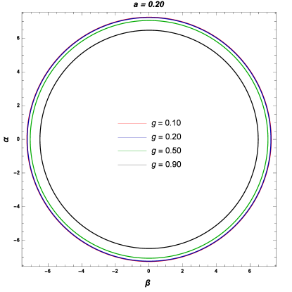
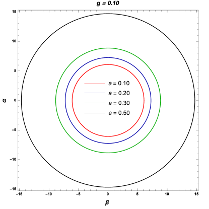
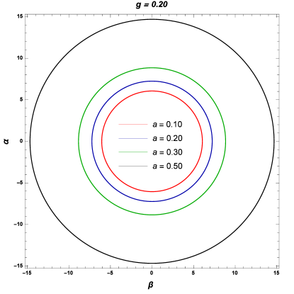
Figure 2: The shadow of a BH for different value of global charge ($a$) and MM charge $g$ for $0.1\,0.2\,\,0.3$ and $a=0.4$ with fixed $M$.

III.2 Quasinormal Modes

Let us consider the QNM of the solution in order to study the dynamical stability of the obtained BH solution (17). It is characterized by the real and imaginary parts of the QNM frequencies, ($\omega=\omega_{R}+i\omega_{I}$). If $\omega>0$, the BH is unstable and $\omega<0$, it is stable. We can compute the QNMs and QNFs by solving the scalar field equation in the black hole space-time Singh:2022xgi ,

$$\frac{1}{\sqrt{-g}}\partial_{\mu}\left(\sqrt{-g}g^{\mu\nu}\partial_{\nu}\right)\phi=0.$$ (26)

The solution can be obtained by separation of variables as,

$$\phi=\frac{1}{r}\sum_{lm}e^{i\omega t}u_{lm}(r)Y^{m}_{l}(\theta,\phi),$$ (27)

where $Y^{m}_{l}$ are spherical harmonics. The radial equation takes the Schrodinger-like form if we use the tortoise co-ordinate $dr^{*}=dr/f(r)$

$$\left(\frac{d^{2}}{dr^{*^{2}}}+\omega^{2}-V_{0}(r^{*})\right)u(r)=0,$$ (28)

where, $V_{0}(r^{*})=f\left(\frac{f^{\prime}}{f}+\frac{l(l+1)}{r^{2}}\right)$.

The QNFs are complex numbers given by $\omega=\omega_{R}+i\omega_{I}$. We use the WKB formula in large $l$ limit will ; iyer ; konoplya1 ; wkb1 ; yar to obtain QNFs.

$$\omega=l\Omega-i\left(n+\frac{1}{2}\right)|\Lambda|,$$ (29)

with

$$\Omega=\frac{\sqrt{f(r_{p})}}{r_{p}}=\frac{1}{L_{p}}\qquad\text{and}\qquad\Lambda=\frac{\sqrt{2f(r_{p})-r^{2}_{p}f^{\prime\prime}(r_{p})}}{\sqrt{2}L_{p}}.$$ (30)

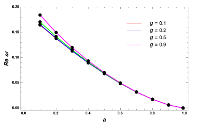
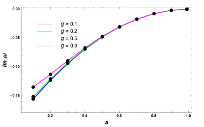
Figure 3: The real (left panel) and imaginary part (right panel) of QNMs for different values of magnetic monopole charge $(g)$ for a fixed value of $M$.

The numerical values of the real and imaginary parts of QNFs are presented in Tab. 4 and 5 and plotted in Fig. 3 for different values of the BH parameters. The negative values of the imaginary part of the QNMs confirm that the modes of the obtained BH are stable.

The effect of parameters ($a,g$) on the behavior of QNMs and QNFs are depicted in Fig. 2. In this Fig. 2, we notice that the real part of the QNMs decreases with $a$ while the imaginary part first increases (becomes less negative) very sharply and then increases slowly (almost constant) with $a$.

	$g=0.1$	$g=0.2$	$g=0.3$	$g=0.4$
$a$	$\omega=\omega_{R}+i\omega_{I}$	$\omega=\omega_{R}+i\omega_{I}$	$\omega=\omega_{R}+i\omega_{I}$	$\omega=\omega_{R}+i\omega_{I}$
0.1	0.1645 - 0.1557 $i$	0.1652 - 0.1553 $i$	0.1663 - 0.1545 $i$	0.1681 - 0.1532 $i$
0.2	0.1378 - 0.1230 $i$	0.1383 - 0.1228 $i$	0.1390 - 0.1223 $i$	0.1401 - 0.1215 $i$
0.3	0.1128 - 0.0942 $i$	0.1130 - 0.0940 $i$	0.1135 - 0.09381 $i$	0.1142 - 0.0933 $i$
0.4	0.0894 - 0.0692 $i$	0.0896 - 0.0691 $i$	0.0899 - 0.0690 $i$	0.0903 - 0.0688 $i$
0.5	0.0680 - 0.0480 $i$	0.0681 - 0.0480 $i$	0.0682 - 0.0479 $i$	0.0685 - 0.0478 $i$
0.6	0.0486 - 0.0307 $i$	0.0487 - 0.0307 $i$	0.0488 - 0.0307 $i$	0.0488 - 0.0307 $i$
0.7	0.0316 - 0.0173 $i$	0.0316 - 0.0173 $i$	0.0316 - 0.0173 $i$	0.0316 - 0.0172 $i$
0.8	0.0172 - 0.0076 $i$	0.0172 - 0.0076 $i$	0.0172 - 0.0076 $i$	0.0172 - 0.0076 $i$
0.9	0.0060 - 0.0019 $i$	0.0060 - 0.0019 $i$	0.0060 - 0.0019 $i$	0.0060 - 0.0019 $i$
0.99	0.0001 - 0.00001 $i$	0.0001 - 0.00001 $i$	0.0001 - 0.00001 $i$	0.0001 - 0.00001 $i$

Table 4: The numerical values of QNMs for various values of CoS parameter, $a$ and magnetic monopole charge, $g$ for a fixed value of $M=1$ (where $l=1$ and $n=0$).

	$g=0.5$	$g=0.6$	$g=0.7$	$g=0.8$
$a$	$\omega=\omega_{R}+i\omega_{I}$	$\omega=\omega_{R}+i\omega_{I}$	$\omega=\omega_{R}+i\omega_{I}$	$\omega=\omega_{R}+i\omega_{I}$
0.1	0.1704 - 0.1513 $i$	0.1736 - 0.1483 $i$	0.1780 - 0.1435 $i$	0.1841 - 0.1349 $i$
0.2	0.1416 - 0.1207 $i$	0.1436 - 0.1189 $i$	0.1462 - 0.1165 $i$	0.1496 - 0.1128 $i$
0.3	0.1151 - 0.0929 $i$	0.1163 - 0.0919 $i$	0.1178 - 0.0907 $i$	0.1197 - 0.0893 $i$
0.4	0.0908 - 0.0685 $i$	0.0915 - 0.0681 $i$	0.0923 - 0.0675 $i$	0.0933 - 0.0668 $i$
0.5	0.0687 - 0.0477 $i$	0.0691 - 0.0475 $i$	0.0695 - 0.0473 $i$	0.0700 - 0.0470 $i$
0.6	0.0490 - 0.0306 $i$	0.0491 - 0.0305 $i$	0.0493 - 0.0304 $i$	0.0495 - 0.0303 $i$
0.7	0.0317 - 0.0172 $i$	0.0317 - 0.0172 $i$	0.0318 - 0.0172 $i$	0.0319- 0.0172 $i$
0.8	0.0172 - 0.0076 $i$	0.0172 - 0.0076 $i$	0.0172 - 0.0076 $i$	0.0172 - 0.0076 $i$
0.9	0.0060 - 0.0019 $i$	0.0060 - 0.0019$i$	0.0060 - 0.0019 $i$	0.0060 - 0.0019 $i$
0.99	0.0001 - 0.00001 $i$	0.0001 - 0.00001 $i$	0.0001 - 0.00001 $i$	0.0001 - 0.00001$i$

Table 5: The numerical values of QNMs for various values of CoS parameter, $a$ and magnetic monopole charge, $g$ for a fixed value of $M=1$ (where $l=1$ and $n=0$).

IV Results and Conclusions

In this article, we considered an exact BH solution of Rodrigue et.el Rodrigues:2022zph ; Rodrigues:2022rfj , when gravity is minimally coupled to NED and CoS source. The size of the black hole (outer) horizon decreases with an increase in magnetic charge, $g$, and increases with CoS parameter, $a$. We studied the photon sphere radii and QNM’s in the eikonal limits. The results showed that the photon sphere radius and shadow radius increases with the CoS parameter and opposite behavior with a magnetic charge. It means that the effect of CoS parameters and magnetic charge are opposite to each other. We also see that the size of the shadow image is bigger than its horizon radius and photon sphere radius.

We employed the well-known connection between the shadow radii Singh:2022dth ; k1 ; k2 ; k3 ; car1 and QNMs. The real part of the QNMs increases with the CoS parameter and decreases with the magnetic charge, which means that the QNM oscillates faster. The imaginary part of the QNM is negative, which means that our BH solution is stable. The imaginary part of the QNM increases with both the CoS parameter and magnetic charge and approaches zero at a very large value of the CoS parameter, which means that the QNMs decayed slower. It would be interesting to study the optical features and mimicker behavior for other solutions such as charged accelerating AdS BHs, $f(R)$ gravity coupled with NED black bounce solutions, regular EGB black holes, $f(Q)$ gravity, and wormhole solutions in CoS background.

- (1) E. S. Fradkin and A. A. Tseytlin, Phys. Lett. B 163 (1985) 123.
- (2) R. Penrose, Phys. Rev. Lett. 14, 57 (1965); S. W. Hawking, Proc. Roy. Soc. Lond. A 300, 187 (1967); S. W. Hawking and R. Penrose, Proc. Roy. Soc. Lond. A 314, 529 (1970).
- (3) K. Jafarzade, M. Kord Zangeneh and F. S. N. Lobo, JCAP 04 (2021), 008
- (4) D. V. Singh, A. Shukla and S. Upadhyay, Annals Phys. 447 (2022), 169157.
- (5) D. V. Singh, V. K. Bhardwaj and S. Upadhyay, Eur. Phys. J. Plus 137 (2022) no.8, 969.
- (6) A. Belhaj, L. Chakhchi, H. El Moumni, J. Khalloufi and K. Masmar, Int. J. Mod. Phys. A 35 (2020) no.27, 2050170.
- (7) B. Eslam Panah, K. Jafarzade and S. H. Hendi, Nucl. Phys. B 961 (2020), 115269.
- (8) E. Ayon-Beato and A. Garcia, Gen. Rel. Grav. 31, 629 (1999).
- (9) E. Ayon-Beato, A. Garcia, Phys. Lett. B 493 (2000) 149.
- (10) J. Bardeen, Proceedings of GR5 (Tiflis, U.S.S.R., 1968).
- (11) S. Fernando, Int. Journal of Mod. Phys. D 26, 1750071 (2017).
- (12) D. V. Singh and N. K. Singh, Annals Phys. 383 (2017), 600-609.
- (13) C. Bambi and L. Modesto, Phys. Lett. B 721, 329 (2013).
- (14) F. Ahmed, D. V. Singh and S. G. Ghosh, Gen. Rel. Grav. 54 (2022) no.2, 21.
- (15) M. Sharif, W. Javed, Can. J. Phys. 89, 1027 (2011).
- (16) D. V. Singh, M. S. Ali and S. G. Ghosh, Int. J. Mod. Phys. D 27 (2018) no.12, 1850108
- (17) T. G. Rizzo JHEP 09, 021 (2006).
- (18) S. G. Ghosh, A. Kumar and D. V. Singh, Phys. Dark Univ. 30 (2020), 100660.
- (19) S. G. Ghosh, D. V. Singh, R. Kumar and S. D. Maharaj, Annals Phys. 424 (2021), 168347.
- (20) D. V. Singh, S. G. Ghosh and S. D. Maharaj, Phys. Dark Univ. 30 (2020), 100730.
- (21) D. V. Singh, S. G. Ghosh and S. D. Maharaj, Annals Phys. 412 (2020), 168025.
- (22) B. K. Singh, R. P. Singh and D. V. Singh, Eur. Phys. J. Plus 135 (2020) no.10, 862.
- (23) B. K. Singh, R. P. Singh and D. V. Singh, Eur. Phys. J. Plus 136 (2021) no.5, 575.
- (24) R. V. Maluf and J. C. S. Neves, Phys. Rev. D 97, 104015 (2018).
- (25) Mang-Sen Ma and Ren Zhao, Class. Quantun Grav. 31 245014 (2014).
- (26) D. V. Singh, S. G. Ghosh and S. D. Maharaj, Annals Phys. 412, 168025 (2020).
- (27) Md. Sabir Ali, S.G. Ghosh, Phys. Rev. D 98, 084025 (2018).
- (28) K. A. Bronnikov, Phys. Rev. D 63 (2001), 044005.
- (29) A. Simpson and M. Visser, arXiv:1911.01020 [gr-qc].
- (30) G. Panotopoulos and A. Rincón, Eur. Phys. J. Plus 134, 300 (2019).
- (31) D. V. Singh, S. G. Ghosh and S. D. Maharaj, Nucl. Phys. B 981 (2022), 115854.
- (32) D. V. Singh and S. Siwach, Phys. Lett. B 808 (2020), 135658.
- (33) Bhupendra Singh, Benoy Kumar Singh, and Dharm Veer Singh, IJGMMP (2023),https://doi.org/10.1142/S0219887823501256.
- (34) A. D. Sakharov, Sov. Phys. JETP 22, 241 (1966).
- (35) N. Tsukamoto, Z. Li and C. Bambi, JCAP 06 (2014), 043.
- (36) P. C. Li, T. C. Lee, M. Guo and B. Chen, Phys. Rev. D 104 (2021) no.8, 084044.
- (37) B. Cuadros-Melgar, R. D. B. Fontana and J. de Oliveira, Phys. Lett. B 811 (2020), 135966.
- (38) Filipe Moura, João Rodrigues, Eikonal quasinormal modes and shadow of string-corrected d-dimensional black holes, Phys. Lett. B 819 (2021), 136407.
- (39) E.B. Gliner, Sov. Phys. JETP 22, 378 (1966).
- (40) M. E. Rodrigues and H. A. Vieira, Phys. Rev. D 106 (2022) no.8, 084015.
- (41) M. E. Rodrigues and M. V. d. S. Silva, Phys. Rev. D 106 (2022) no.8, 084016.
- (42) K. Akiyama et al., Astrophys. J. 875 L1 (2019).
- (43) K. Akiyama et al, Astrophys. J. 875, L4 (2019).
- (44) P. S. Letelier, Phys. Rev. D 28, 2414 (1983).
- (45) P. S. Letelier, Phys. Rev. D 20, 1294 (1979).
- (46) P. S. Letelier, Il Nuovo Cim. B 63 519 (1981).
- (47) J. L. Synge, Relativity: The General Theory, (North Holland, Amsterdam, 1966), p. 175.
- (48) A. Belhaj, H. Belmahi, M. Benali, W. El Hadri, H. El Moumni and E. Torrente-Lujan, Phys. Lett. B 812 (2021), 136025.
- (49) A. Belhaj and Y. Sekhmani, Gen. Rel. Grav. 54 (2022) no.2, 17.
- (50) A. Belhaj, H. Belmahi, M. Benali and A. Segui, Phys. Lett. B 817 (2021), 136313.
- (51) V. Perlick, O. Y. Tsupko and G. S. Bisnovatyi-Kogan, Phys. Rev. D 92 (2015) no.10, 104031.
- (52) B. F. Schutz and C. M. Will, Astrophys J. 291 L33 (1985).
- (53) S. Iyer and C. M. Will, Phys. Rev. D 35, 3621(1987).
- (54) R. A. Konoplya, Phys. Rev. D 68, 024018 (2003).
- (55) Yerlan Myrzakulov, Kairat Myrzakulov, Sudhaker Upadhyay, and Dharm Veer Singh, International Journal of Geometric Methods in Modern Physics (2023).
- (56) V. Cardoso, A. S. Miranda, E. Berti, H. Witek and V. T. Zanchin, Phys. Rev. D 79 (2009) no.6, 064016.
- (57) D. V. Singh, V. K. Bhardwaj and S. Upadhyay, Eur. Phys. J. Plus 137 (2022) no.8, 969.
- (58) K. Jusufi, Phys. Rev. D 101, 084055 (2020).
- (59) K. Jusufi, Phys. Rev. D 101 124063 (2020).
- (60) R. A. Konoplya and Z. Stuchlík, Phys. Lett. B 771 (2017), 597-602.
- (61) V. Cardoso, A. S. Miranda, E. Berti, H. Witek, V. T. Zanchin, Phys. Rev. D 79 (2009) 064016.