Rotation and activity in late-type members of the young cluster ASCC  123

Abstract

ASCC 123 is a little-studied young and dispersed open cluster. Recently, we conducted the first research devoted to it. In this paper, we complement our previous work with TESS photometry for the 55 likely members of the cluster. We pay special attention to seven of these high-probability members, all with FGK spectral types, for which we have high-resolution spectra from our preceding work. By studying the TESS light curves of the cluster members we determine the rotational period and the amplitude of the rotational modulation for 29 objects. The analysis of the distribution of the periods allows us to estimate a gyrochronogical age for ASCC 123 similar to that of the Pleiades, confirming the value obtained in our previous investigation. A young cluster age is also suggested by the distribution of variation amplitudes. In addition, for those stars with spectroscopic data we calculate the inclination of their rotation axis. These values appear to follow a random distribution, as already observed in young clusters, with no indication of spin alignment. However, our sample is too small to confirm this on more solid statistical grounds. Finally, for these seven stars we study the level of magnetic activity from the H$\alpha$ and Ca ii H&K lines. Despite the small number of data points, we find a correlation of the H$\alpha$ and Ca ii flux with Rossby number. The position of these stars in flux–flux diagrams follows the general trends observed in other active late-type stars.

1 Introduction

Stellar rotation and magnetic activity are properties strongly related to the evolution of stars, from the pre-main to the post-main sequence. During the main sequence (MS) phase, the position of a star on the Hertzsprung-Russell (HR) diagram changes very little, so it is not an efficient indicator of stellar age. Conversely, the rotation rate and the level of magnetic activity, which is closely related to the rotation speed, change significantly over the life of a star in the main sequence due to the magnetic braking. The latter is caused by the angular momentum carried off by magnetized stellar wind.

Since the pioneering work of Skumanich (1972), who discovered the empirical law that bears his name, of the decline of the equatorial rotation speed with the inverse square root of the star’s age, the rotation rate and magnetic activity have been used to estimate the age of stars in the solar neighbourhood (e.g., Barry et al., 1987; Soderblom et al., 1991; Barnes, 2003; Barnes et al., 2016; Stanford-Moore et al., 2020, and references therein). Another widely used age indicator is the atmospheric abundance of lithium (e.g., Jeffries, 2014; Gutiérrez Albarrán et al., 2020, and references therein).

On the other hand, rotation and activity can also be used as additional criteria, along with the kinematics, lithium abundance, and the position in the HR diagram, for evaluating the probability for a star to be member of an open cluster. This can be of great help in the case of stars in the halo of young clusters or very dispersed clusters. This is the case of ASCC 123, a young and poorly studied cluster. ASCC 123 was discovered by Kharchenko et al. (2005) based on $Hipparcos$ proper motions and $BV$ archival photometry. They found 24 likely members spread over a large region of more than 2 degrees on the sky. They found a low reddening, $E(B-V)=0.10$, placed the cluster at a distance of 250 pc, and estimated an age of about 260 Myr. The parameters of this cluster were subsequently reanalyzed by Yen et al. (2018) on the basis of the $Gaia$ DR1/TGAS and HSOY data (Altmann et al., 2017). They confirmed the low reddening, $E(B-V)=0.097$, a distance $d$=243.5 pc, and revised the cluster age as $\tau=130$ Myr. Cantat-Gaudin et al. (2018), from the $Gaia$ DR2 astrometric and photometric data, reported 55 cluster members and estimated a distance of $233.1\pm 5.5$ pc.

In our previous work (Frasca et al., 2019, hereafter Paper I), we studied some of the brightest candidate members of ASCC 123 using high-resolution spectra obtained with HARPS-N at the Telescopio Nazionale Galileo (TNG) with the aim of determining their physical parameters, radial and rotational velocities, and the abundances of some elements. The chemical composition of this cluster turned out to be compatible with the Galactic trends in the solar neighbourhood. The HR and colour-magnitude diagrams (CMDs), as well as the lithium abundance and the H$\alpha$ emission allowed us to infer an age in the range 100–200 Myr, i.e. similar to that of the Pleiades.

In the present paper we use ground-based and TESS photometry for the members of ASCC 123 to investigate their photospheric activity and study the distribution of their rotation periods. We use also the HARPS-N spectra already gathered to derive the level of magnetic activity from the H$\alpha$ and Ca ii H&K lines and the projected rotational velocity ($v\sin i$) to derive the inclination of the rotation axes. The paper is organised as follows. In Sect. 2 we present the observations and the criteria followed to select our targets. In Sect. 3 we show the results of our work, describing the analysis carried out on both the photometric and spectroscopic data. We discuss our results and compare our findings with other clusters in Sect. 4. Finally, Sect. 5 summarizes the main results and presents our conclusions.

2 Observations and data reduction

2.1 Spectroscopy

In this paper we investigate the chromospheric activity for the single, late-type stars studied in Paper I that are bona-fide members (i. e. with a membership probability $Prob$=1) according to Cantat-Gaudin et al. (2018). For these seven FGK stars we follow the same numbering used in our previous work (ID). We use high-resolution spectra taken in 2018 and 2019 with GIARPS (GIANO-B & HARPS-N; Claudi et al. 2017) at the 3.6m TNG telescope. The reader is referred to Paper I for a description of the data and their reduction. The analysis of these spectra with the code ROTFIT, aimed at the determination of the atmospheric parameters and $v\sin i$, can be also found in Paper I.

Table 1: Stellar parameters of the late-type members of ASCC 123 from Frasca et al. (2019) and from the present work.

ID	TIC	RA	DEC	$T_{\rm eff}$	err	SpT	$v\sin i$	err	$M_{*}$	$R_{*}$	$P_{\rm rot}$	err	$i$
		(J2000)	(J2000)	(K)			(km s-1)		($M_{\odot}$)	($R_{\odot}$)	(days)		($\degr$)
39	64837857	22 35 13.26	+54 46 24.8	6667	115	F4V	49.1	1.9	1.38	1.36	1.67:	…	$\sim 90$
214	249784843	22 38 34.03	+53 35 08.7	5804	87	G1.5V	100.9	3.0	1.09	1.16	0.562	0.002	75${}^{+11}_{6}$
435	388696341	22 42 00.19	+55 00 58.5	5758	79	G2.5V	11.6	0.7	1.07	0.96	3.92	0.02	69${}^{+15}_{10}$
517	428274538	22 43 26.53	+54 11 58.4	5784	81	G2V	83.6	1.9	1.08	1.13	0.579	0.002	58${}^{+2}_{3}$
554	361944360	22 44 00.20	+54 08 38.1	6871	152	F4V	81.8	3.3	1.46	1.40	0.857	0.007	81${}^{+9}_{10}$
F1	66539637	22 45 28.25	+53 47 06.1	5263	92	K0V	6.6	0.6	0.94	0.92	5.83	0.05	56${}^{+9}_{8}$
F2	64077901	22 31 17.98	+55 02 40.7	5237	77	K1V	7.5	0.6	0.93	0.88	5.09	0.05	59${}^{+10}_{8}$

Table 1 reports the ID of the observed targets along with the TESS Input Catalog (TIC, Stassun et al. 2019; Paegert et al. 2022) identifier, equatorial coordinates (RA, DEC), effective temperature ($T_{\rm eff}$), spectral type (SpT) and $v\sin i$, which were already derived in Paper I. The masses ($M_{*}$) and radii ($R_{*}$), reported in columns 10 and 11 of Table 1, have been derived from the comparison of the position of these stars in the HR diagram (Figure 8 in Paper I) with the PARSEC isochrones ($age$=155 Myr) and evolutionary tracks (Bressan et al., 2012). The rotation period ($P_{\rm rot}$) measured from the analysis of TESS light curves (Sect. 3.1) and the inclination ($i$) of the rotation axis, calculated as described in Sect. 4.3, are also quoted in the last columns of Table 1.

2.2 Photometry

Space-born accurate photometry was obtained with NASA’s Transiting Exoplanet Survey Satellite (TESS; Ricker et al. 2015) for all the cluster members identified by Cantat-Gaudin et al. (2018), 55 stars in total. Our targets were observed by TESS in sector 16, between 2019-09-12 and 2019-10-06, and sector 17, between 2019-10-08 and 2019-11-02. The observations in two consecutive sectors allowed us to obtain nearly uninterrupted sequences (with a gap of about 1.4 days) of high-precision photometry lasting about 50 days, with a cadence of 30 minutes. Being ASCC 123 a sparse and nearby cluster, there is no severe star crowding, also taken the large pixel size of TESS (21″) into account. Indeed, searching in the Gaia DR3 catalogue (Gaia Collaboration, 2022), no star with a comparable magnitude ($\Delta G<2$ mag) can be found within a radius of 21″around the position of each target. Therefore, we expect no relevant flux contamination from nearby sources. We downloaded the TESS light curves (Huang et al., 2020) from the MAST archive and used the Simple Aperture Photometry flux (SAP) or the Pre-search Data Conditioning SAP flux (PDCSAP), where long term trends have been removed, whenever available. For the targets fainter than about $V=14$ mag we used the TESS light curves extracted with a PSF-based approach (PATHOS, Nardiello et al. 2019).

We have also performed multiband $BVR_{\rm C}I_{\rm C}$ photometric observations with the facility imaging camera at the 0.91 m telescope of the M. G. Fracastoro station (Serra La Nave, Mt. Etna, 1735 m a.s.l.) of the Osservatorio Astrofisico di Catania (OACT, Italy). We observed the three G-type members in our sample, namely S 214, S 435, and S 517 during 9 nights from 22 October 2019 to 16 January 2020, collecting from 23 to 29 data points per each filter and per each star. Time series data covering about 3–4 hours could be acquired only on 23 October, 4 and 20 November 2019. We decided to start observing S 214 and S 517 because of their large $v\sin i$, which would imply a rotation period short enough and a modulation amplitude large enough to be able to detect brightness variations with observations from the ground. S 435 was included as a test target because of its spectral type similar to the other two fast-rotating stars. We did not consider the fast-rotating F4V stars S 39 and S 554 for which we expected small variation amplitudes that are hardly detectable from the ground. We used exposure times of 60, 30, 15, and 15 sec for the $B$, $V$, $R_{\rm C}$, and $I_{\rm C}$ band, respectively. The data were reduced by subtracting master darks taken with the same exposure times as the science images and by dividing them by master flats. Aperture photometry with a radius of 6 pixels ($\simeq 4\arcsec$) was performed for the unsaturated stars in the field of view of 11.2${}^{\prime}\times 11.2^{\prime}$ of each of the observed targets. Standard stars in the open cluster NGC 7790 (Stetson, 2000) were also observed in the nights with the best photometric conditions to calculate the zero points and transformation coefficients to the Johnson-Cousins system. With the latter we calculated the $BVR_{\rm C}I_{\rm C}$ magnitudes for a number of non-variable stars in each target field that have been used as comparison for doing ensemble photometry of the monitored stars. Although the precision and cadence from this ground-based photometry is not comparable to that of TESS, these multiband data are useful to determine average magnitudes and colours for these three targets. Since in the meantime TESS had started to observe the sky region containing ASCC 123 providing a very precise photometry (although with no colour information), we decided not to continue with the observations from the ground.

The main results presented in this paper are based on the TESS photometry only. For the sake of completeness, we report the results of ground-based photometry in Appendix A.

3 Data analysis and results

3.1 TESS light curves

Table 2: Rotation periods and variation amplitudes for the members of ASCC 123 derived in the present work.

TIC	RA	DEC	Sourcea	$G^{a}$	$G_{\rm BP}-G_{\rm RP}^{a}$	$V^{b}$	$K_{\rm S}^{c}$	Probd	Ampl	$P_{\rm rot}$	err
	(J2000)	(J2000)		(mag)	(mag)	(mag)	(mag)		(mag)	(days)
467546937	22 29 27.77	+53 16 35.4	2001745344554471296	16.062897	2.862838	17.233	12.225	1.0	0.0726	5.40	0.26
249784843	22 38 34.03	+53 35 08.7	2003023629898711680	11.816078	0.914368	12.187	10.194	1.0	0.0836	0.562	0.002
428062248	22 36 24.68	+53 15 06.1	2003011500910639744	15.950929	2.474563	16.461	12.419	1.0	…	…	…
452862919	22 34 35.38	+53 05 22.0	2002983291564863872	17.446210	2.999275	17.970	13.511	1.0	…	…	…
66541342	22 46 07.28	+53 30 19.7	2002130929538238336	15.743083	2.433725	16.906	12.153	1.0	0.0285	6.22	0.81
66541343	22 46 06.80	+53 30 19.2	2002130929538237952	17.163408	3.006250	…	13.104	0.8	…	…	…
298019363	22 51 06.72	+54 28 54.2	2002757891681122944	17.132408	3.015108	17.150	13.098	0.8	…	…	…
427062959	22 39 36.92	+53 07 03.0	2002201225257443072	13.165830	1.231491	13.503	11.045	1.0	0.0461	5.29	0.02
64073268	22 30 24.04	+54 08 38.9	2001844163164756992	17.318691	3.011692	17.970	13.382	0.6	…	…	…
197755998	22 28 01.49	+53 47 39.9	2001820798541996928	17.113846	2.967771	…	13.178	0.9	…	…	…
361944444	22 44 20.64	+54 10 08.3	2002409582707022592	17.910720	3.171944	…	13.869	0.8	…	…	…
361944360	22 44 00.20	+54 08 38.1	2002409483936262016	10.176037	0.637021	10.410	9.168	1.0	0.0024	0.857	0.007
66194421	22 43 13.83	+53 53 46.0	2002397698545886592	16.360283	2.723582	17.692	12.595	0.8	0.2267	2.15	0.06
428274538	22 43 26.53	+54 11 58.4	2003161751738142464	11.994698	0.997400	12.199	10.205	1.0	0.0517	0.579	0.002
64838038	22 34 51.43	+54 43 20.3	2003377530902056064	17.930496	3.233290	…	13.856	0.9	…	…	…
64837857	22 35 13.26	+54 46 24.8	2003378188041736320	10.356592	0.619606	10.385	9.291	1.0	0.0051	1.67	0.01
343437865	22 46 13.51	+53 59 10.6	2002718377980766336	17.758833	3.240006	…	13.636	0.8	…	…	…
317272583	22 48 38.34	+54 44 01.6	2002822934667425408	17.820822	3.080757	…	13.742	0.7	…	…	…
317273771	22 48 47.90	+54 24 53.6	2002801150593176064	6.112235	-0.092576	6.134	6.310	1.0	…	…	…
367686364	22 55 46.32	+54 57 08.8	2002876535856254464	10.035475	0.606720	10.255	9.050	0.8	0.0023	4.37	0.08
67055292	22 50 14.85	+53 33 28.1	2002471537620861056	16.707653	2.859225	17.560	12.819	0.9	…	…	…
64647628	22 34 50.16	+54 10 04.2	2003297923690672512	15.213570	2.429640	16.294	11.692	1.0	0.0588	2.71	0.08
64278003	22 31 36.44	+54 04 19.3	2003330050047078144	17.137224	3.127945	…	13.098	1.0	…	…	…
64077901	22 31 17.98	+55 02 40.7	2006435105245732480	12.769458	1.083085	12.805	10.839	1.0	0.0961	5.09	0.05
415468735	22 29 36.22	+55 16 16.8	2006455961606619520	13.152347	1.193418	13.399	11.100	1.0	0.0291	3.99	0.03
64561694	22 33 59.64	+55 42 22.4	2006489462352825344	15.635015	2.427858	16.505	12.067	0.6	0.1949	6.61	0.45
317271523	22 48 25.68	+55 01 22.3	2003593864116296576	16.727818	2.879941	17.800	12.902	1.0	…	…	…
416319381	22 37 50.00	+56 11 54.5	2006619303494467328	17.878110	3.284651	…	13.790	0.6	…	…	…
249725057	22 37 01.79	+53 34 52.1	2003031841875970176	16.084180	2.522219	17.232	12.480	1.0	…	…	…
388387063	22 40 14.32	+54 32 27.7	2003216972147204608	13.000790	1.158239	13.382	10.930	1.0	0.0534	3.19	0.03
64646728	22 33 35.99	+53 58 10.4	2003271397972097024	13.680970	1.375657	13.911	11.279	1.0	0.0799	4.03	0.07
388651771	22 40 48.14	+54 35 46.6	2003240920885298176	17.222970	2.861937	17.820	13.303	0.9	…	…	…
420123691	22 32 07.17	+53 42 26.4	2003259372063199744	13.262769	1.266625	13.594	11.053	1.0	0.4418	13.43	0.20
388693014	22 41 34.98	+54 35 30.0	2003228517019770240	17.371294	3.338816	…	13.166	0.9	…	…	…
431151968	22 41 18.32	+53 17 51.3	2002297368107185920	16.220058	2.902960	17.080	12.348	0.8	0.0787	0.910	0.015
66343379	22 44 17.19	+53 35 24.7	2002328875988217216	16.020758	2.592554	17.219	12.356	1.0	0.0456	4.98	0.30
66539637	22 45 28.25	+53 47 06.1	2002337603362057088	12.563967	1.053528	12.669	10.649	1.0	0.0483	5.83	0.05
2046168414	22 45 28.58	+53 47 07.9	2002337603353142016	17.408490	1.998825	18.077	10.649	0.6	…	…	…
420304656	22 40 23.86	+53 49 07.6	2003120764877992448	17.124058	2.955116	17.970	13.259	0.8	…	…	…
431150096	22 41 28.14	+53 52 51.6	2003127705545276032	12.836430	1.113888	12.977	10.868	1.0	0.0697	5.24	0.06
2046389820	22 41 06.01	+53 59 05.8	2003132344098378496	14.223695	…	…	…	0.7	…	…	…
452865760	22 34 58.37	+53 56 32.2	2003104718883916288	17.162186	3.024750	17.610	13.226	0.7	…	…	…
427060252	22 39 36.76	+53 52 53.3	2003136501637932672	15.955221	2.871970	16.900	12.065	0.8	0.0451	0.367	0.003
66723344	22 47 59.13	+53 40 15.4	2002508302542111488	16.220280	2.973432	17.560	12.251	0.9	0.0292	0.311	0.002
67224655	22 52 17.23	+53 53 39.2	2002528402990066944	15.586474	2.455151	16.671	11.949	0.9	0.1094	1.737	0.031
297927402	22 50 32.54	+54 02 14.8	2002543967951224960	16.304932	2.683093	17.568	12.476	0.9	0.0515	1.503	0.023
343771372	22 46 34.54	+54 46 05.2	2003554006818945280	9.578720	0.443725	9.703	8.837	0.9		…	…
2015953058	22 31 48.85	+54 59 22.7	2006387242128323840	14.283266	1.744160	14.416	10.775	1.0	0.0965	5.19	0.04
64077487	22 30 51.98	+54 55 50.1	2006385764659269760	16.194597	2.755547	17.110	12.358	0.6	0.0445	3.52	0.26
67062121	22 50 59.10	+53 19 00.0	2002452708484342656	17.461884	2.946167	17.970	13.457	0.8	…	…	…
388696341	22 42 00.19	+55 00 58.5	2003443437181978240	12.048476	0.941633	12.261	10.418	1.0	0.0838	3.92	0.02
343867253	22 47 52.68	+55 33 18.5	2003669180664786944	15.195872	2.754218	15.750	11.370	0.8	0.0305	0.464	0.003
343778985	22 47 36.61	+55 10 30.5	2003645060128342656	16.949617	2.980359	17.800	12.994	0.6	…	…	…
431153083	22 41 11.77	+52 56 27.8	2002274106564094848	13.922489	1.505455	14.256	11.335	1.0	0.0780	6.90	0.03
249801592	22 39 19.22	+53 29 16.5	2002270842392282496	10.599697	0.758198	10.765	9.314	1.0	…	…	…

Notes. ^a From Gaia DR3 catalogue (Gaia Collaboration, 2022). ^b From TESS Input Catalog (Paegert et al., 2022). ^c From 2MASS catalogue (Skrutskie et al., 2006). ^d Membership probability according to Cantat-Gaudin et al. (2018).

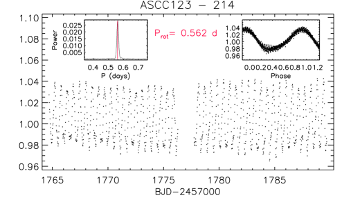
Figure 1: TESS light curve of S 214 (TIC 249784843) in 2019 (sector 17). The inset in the upper left corner shows the cleaned periodogram of these data; the rotational period is marked with a vertical red line. The inset in the upper right corner displays the data phased with this period.

The main information we can get from the TESS light curves is the rotation period, $P_{\rm rot}$, of the star, which can be measured thanks to the rotational modulation of the star’s brightness produced by an uneven distribution of cool photospheric spots. The amplitude of the photometric variations is also a useful parameter related to the magnetic activity.

To measure $P_{\rm rot}$ we have applied a periodogram analysis (Scargle, 1982) and the CLEAN deconvolution algorithm (Roberts et al., 1987) to the TESS light curves of the members of ASCC 123. For the stars with periods longer than a few days, we merged the data of sectors 16 and 17 to expand the time base so as to improve the precision of the period determination. Ultrafast rotators, such as S 214 and S 517, display a substantial starspot evolution during the 50-days time baseline, so that for these stars we have preferred to analyse independently sectors 16 and 17, obtaining always very similar values of $P_{\rm rot}$  in the two epochs.

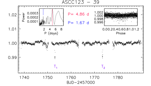
Figure 10: TESS light curve of S 39 (TIC 64837857) in 2019 (sectors 16 and 17). The two transits are marked with T₁ and T₂. The inset in the upper left corner shows the cleaned periodogram of the data excluding the transits; the period corresponding to the maximum power is marked with a vertical red line and is written next to the box. The blue vertical line marks the possible rotational period of about 1.67 days. The inset in the upper right corner displays the data phased with this period.

We retrieved the TESS light curves for the 55 candidate members of the cluster ASCC 123 according to Cantat-Gaudin et al. (2018) but we were able to determine the rotation period only for 29 of them. Indeed, we rejected the stars with Gaia magnitude $G>16.5$, whose TESS photometry is too noisy for a meaningful measure of the rotation period. Moreover, we discarded the objects that we recognized as double-lined binaries (SB2) in Paper I. All the periods are reported in Table 2. For illustrative purposes, the TESS light curve and the result of the period search for S 214 is shown in Fig. 1. The light curves of the remaining FGK members studied in Paper I are displayed in Figs. 10 to 16. The modulation of the star brightness produced by the spots and star rotation is clearly visible for all the targets; exceptions are the two hottest sources. Interestingly, the light curve of S 39 clearly displays two dips reminiscent of a planet transit with a time separation of about 20.31 days (see also Fig. 11). When we started the present investigation, this star was not known to host exoplanets and was not included in the list of TESS Objects of Interest (TOIs). We have then proposed this source for the TESS Follow-up Observing Program (TFOP) and we are planning ground-based observations, whose results will be presented in a forthcoming work. To search for the rotational period of S 39, we excluded the two transits from the TESS light curve obtained merging those of sector 16 and 17 before applying the period analysis.

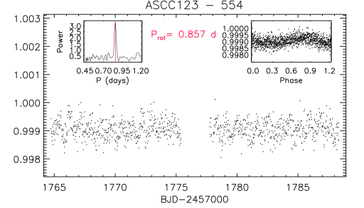
Figure 13: TESS light curve of S 554 (TIC 361944360) in 2019 (sector 17). The figure layout is the same as Fig. 12.

We note that the cleaned periodograms display for all the stars but S 39 a clear power peak (marked with a red vertical line in each plot) without secondary peaks of comparable amplitude. This period thus represents the rotational one. Even the hottest star, S 554, displays a significant rotational modulation, although with a very low amplitude of only $\sim$ 0.007 mag, which is clearly shown by the phased light curve displayed in the right inset panel of Fig. 13. As mentioned above, the only doubtful case is S 39, for which the highest power in the periodogram is found at a period 4.86 days, which is clearly inconsistent with the rapid rotation of the star indicated by the high value of the projected rotation velocity, $v\sin i$$\simeq 49$ km s^-1. However, the periodogram displays other peaks at about 7 days (which is still more inconsistent with the $v\sin i$) and at 1.67 days (marked with a blue vertical line in the left inset panel of Fig. 10); we consider the last as a possible $P_{\rm rot}$ value and list it in Table 1 with a colon.

3.2 Chromospheric emission

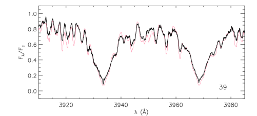
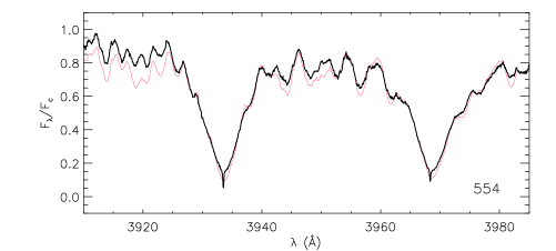
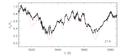
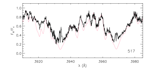
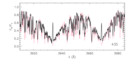
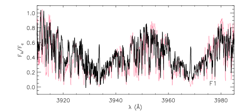
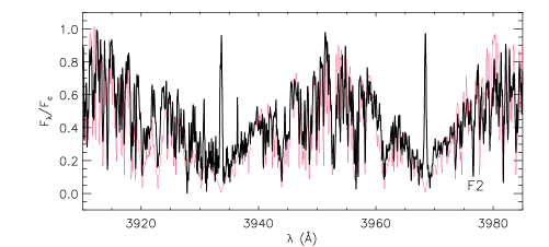
Figure 2: HARPS-N spectra of the investigated stars in the Ca ii H&K region. In each box, the non-active template (red line) is overlaid with the observed spectra (thick black line). The ID of the source is marked in the lower right corner of each box. The two uppermost panels display the hottest (F4V-type) stars in our sample for which no clear emission in the H&K line cores is visible.

The level of chromospheric activity can be evaluated from the emission in the core of the H$\alpha$ and Ca ii H and K lines (see, e.g., Frasca & Catalano, 1994; Frasca et al., 2010; Frasca et al., 2019, and references therein). To this end, we subtracted photospheric templates from the observed spectra of the targets, to remove the underlying photospheric absorption lines so as to leave as residual the chromospheric emission in the cores of H$\alpha$ and Ca ii lines. The photospheric templates are made with synthetic BTSettl spectra (Allard et al., 2012), for Ca ii lines, and spectra of non-active stars for the H$\alpha$; indeed the latter are better reproducing the core of the H$\alpha$ line in absence of a significant chromospheric contribution. Since the signal-to-noise ratio in the Ca ii H & K region is quite low, ranging from 3 (for the coolest members) to 38 (for the hottest one), we have degraded the original resolution (R=115,000) of the HARPS-N spectra and the synthetic spectra to R=42,000, which is the same of the ELODIE templates used for the determination of the atmospheric parameters and the subtraction of the photospheric H$\alpha$ template (Paper I). Furthermore, the photospheric templates have been aligned in wavelength with the target spectra by means of the cross-correlation function and have been rotationally broadened by the convolution with a rotational profile with the $v\sin i$ of the target star (Table 1).

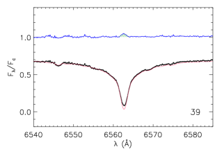
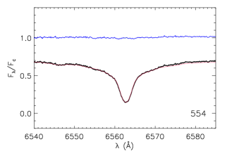
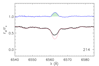
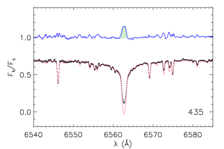
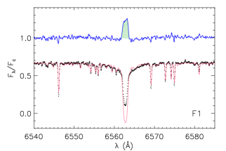
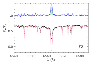
Figure 17: HARPS-N spectra of the investigated stars in the H$\alpha$ region. In each box, the non-active template (red line) is overlaid with the observed spectrum (black dots). The chromospheric emission which fills in the H$\alpha$ core is clearly visible in the subtracted spectrum (blue line in each panel). The green hatched area represents the excess H$\alpha$ emission that was integrated to obtain $W_{\rm H\alpha}$. The ID of the source is marked in the lower right corner of each box.

The observed spectra (black lines) and the photospheric templates (red lines) are displayed in Fig. 2 for the Ca ii H & K region. Figure 17 shows the H$\alpha$ profiles of the targets (black dots) overlaid to the photspheric templates (red lines) and the difference of the two (blue lines). The excess H$\alpha$ equivalent width, $W_{\rm H\alpha}$, has been obtained by integrating the residual H$\alpha$ emission profile, which is highlighted by the green hatched areas in the difference spectra in each box of Fig. 17. Analogously, for each target, the difference between observed and template spectrum in the Ca ii region leaves emission excesses in the cores of the H and K lines, which have been integrated obtaining the equivalent widths, $W_{\rm CaII-H}$ and $W_{\rm CaII-K}$. It is worth noticing that the hottest star in our sample, S 554 ($T_{\rm eff}$=6871 K), does not show any filling in the H$\alpha$ core and only a tiny filling in the cores of the Ca ii lines (upper right panels in Figs. 17 and 2). For S 39 ($T_{\rm eff}$=6667 K) a small residual emission is detected in the core of the H$\alpha$ and also in the Ca ii lines. However, unlike the other stars of lower temperature, no reversal in emission emerges in the cores of the H and K lines for these two F4-type stars. This is in line with what is expected on the basis of the reduced chromospheric activity in these stars with shallow convective envelopes and the difficulty of detecting low chromospheric emission against a large continuum flux.

As a more effective indicator of chromospheric activity, we computed the surface flux in each of the chromospheric lines, $F_{\rm line}$. For the Ca ii K line this reads as

$$F_{\rm CaII-K}=F_{3933}W_{\rm CaII-K},$$ (1)

where $F_{3933}$ is the flux at the continuum at the center of the Ca ii K line per unit stellar surface area, which is evaluated from the BTSettl spectra (Allard et al., 2012) at the stellar temperature and surface gravity of the target. We evaluated the flux error by taking into account the error of $W_{\rm CaII-K}$ and the uncertainty in the continuum flux at the line center, $F_{3933}$, which is estimated considering the errors of $T_{\rm eff}$  and $\log g$.

We computed surface fluxes for the other chromospheric diagnostics in the same way as for the Ca ii-K line. The EWs and fluxes are reported in Table 3.

Table 3: H$\alpha$ and Ca ii H & K equivalent widths and fluxes.

ID	$T_{\rm eff}$	$W_{\rm H\alpha}$	err	$F_{\rm H\alpha}$	err	$W_{\rm CaII-K}$	err	$W_{\rm CaII-H}$	err	$F_{\rm CaII-K}$	err	$F_{\rm CaII-H}$	err
	(K)	(mÅ)		(erg cm-2s-1)		(mÅ)		(mÅ)		(erg cm-2s-1)		(erg cm-2s-1)
39	6667	73	13	9.01e+05	1.69e+05	189	65	145	55	3.42e+06	1.23e+06	2.62e+06	1.05e+06
214	5804	291	21	2.17e+06	1.99e+05	853	122	780	127	5.03e+06	1.04e+06	4.60e+06	1.02e+06
435	5758	144	18	1.04e+06	1.40e+05	492	74	438	80	2.73e+06	5.17e+05	2.43e+06	5.27e+05
517	5784	591	33	4.34e+06	3.31e+05	1082	211	985	232	6.18e+06	1.40e+06	5.63e+06	1.48e+06
554	6871	…	…	…	…	64	22	64	20	1.45e+06	5.32e+05	1.43e+06	4.83e+05
F1	5263	196	22	9.93e+05	1.33e+05	519	155	443	174	1.34e+06	4.57e+05	1.15e+06	4.87e+05
F2	5237	396	30	1.96e+06	1.93e+05	786	194	608	250	1.94e+06	5.54e+05	1.50e+06	6.55e+05

4 Discussion

4.1 Rotational periods

The distribution of rotation periods as a function of the stellar mass is a very useful tool for characterising the evolutionary stage of a cluster (e.g. Barnes, 2003, and references therein). To this aim, we plot in Fig. 3a the periods listed in Table 2 versus the colour index $(G_{\rm BP}-G_{\rm RP})_{0}$, which has been dereddened using the value $A_{V}=0.13$ mag derived in Paper I and the extinction relations in Wang & Chen (2019). In the same plot we also show the periods derived by Rebull et al. (2016) for a sample of Pleiades members observed with Kepler-K2. To compare our period distribution with previous works devoted to other clusters we also use the colour index $(V-K_{\rm s})_{0}$ in Fig. 3b. Despite the small data sample, the rotation periods for the candidate members of ASCC 123 roughly follow the distribution of the Pleiades, with the presence of both fast and slow rotators for G-type stars. We note that, among the three solar-like stars, S 214 and S 517 lie in the fast-rotating C sequence (according to the notation of Barnes 2003), while S 435 falls on the I sequence of the Pleiades, for which the period increases steadily with the colour index up to $(G_{\rm BP}-G_{\rm RP})_{0}\approx 1.5$ mag and then decreases reaching the C sequence at $(G_{\rm BP}-G_{\rm RP})_{0}\approx 3$ mag. We do not find fast rotators (in the lower C sequence) with colour $1<(G_{\rm BP}-G_{\rm RP})_{0}<2.5$, i.e. approximately in the spectral-type range G3–M3. However, the presence of the two fast-rotating solar-type stars strongly supports a young age for the cluster, because the C sequence of older clusters like NGC 3532 (age$\sim$300 Myr) displaces towards cooler objects (e.g., Barnes, 2003; Fritzewski et al., 2021) and practically disappears for the still older Hyades or Praesepe clusters (Barnes, 2003; Rebull et al., 2022), i.e. at age $\approx$ 600 Myr. Indeed, the hottest stars in NGC 3532 with $P_{\rm rot}<1$ day have a $(V-K_{\rm s})_{0}\simeq 3$ (Fritzewski et al., 2021). Another cluster in the age range between the Pleiades and the Hyades is M 48. For this cluster, with an age of about 450 Myr, Barnes et al. (2015) found no G- or early K-type fast rotating stars. A younger cluster showing a clear C sequence reaching the G-type stars is M 34 (age$\sim$250 Myr, Ianna & Schlemmer, 1993). Therefore, the gyrochronogical age of ASCC 123 should not be greater than 250–300 Myr.

As a further check, we have also plotted in Fig. 3 rotational isochrones calculated for slow-rotator sequences by Spada & Lanzafame (2020) and expressed as a function of stellar mass or $B-V$ in their Table A.1. For this purpose, we have converted the $B-V$ colour index into $V-K_{S}$ and $G_{\rm BP}-G_{\rm RP}$ according to the calibrations of Mamajek. As apparent, the $I$ sequences of both ASCC 123 and the Pleiades agree with the theoretical isochrone of Spada & Lanzafame (2020) with the smallest age in their model ($\tau=100$ Myr).

On the other hand, a much younger age seems to be ruled out by the clear gap between fast and slow rotators observed for ASCC 123. Indeed, this gap is not visible in very young ($\approx 16$ Myr) stellar populations, such as the Upper Centaurus-Lupus (UCL) and Lower Centaurus-Crux (LCC) (Rebull et al., 2022). The most discrepant object, with respect to the Pleiades diagram, is TIC 420123691, for which we measure a period of 13.4 days that places it much higher than the Pleiades I sequence. This object could be a non-member or a close binary.

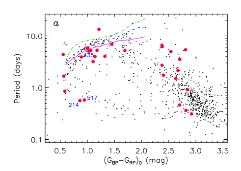
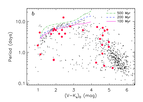
Figure 3: (a) Rotation periods versus the dereddened colour index $(G_{\rm BP}-G_{\rm RP})_{0}$ for the candidate members of the cluster ASCC 123 selected by Cantat-Gaudin et al. (2018) (red circles). Small black dots denote the periods derived for a sample of Pleiades members by Rebull et al. (2016) during the Kepler-K2 campaign. The ID of the three solar-like stars is also marked. Rotational isochrones from Spada & Lanzafame (2020) at ages of 100, 200, and 500 Myr are over-plotted with continuous, dashed, and dash-dotted lines, respectively. (b) Rotation periods versus $(V-K_{\rm s})_{0}$.

4.2 Variation amplitudes

Another proxy for the magnetic activity level is the amplitude of photometric variations induced by starspots (see, e.g. See et al., 2021; Messina, 2021). The variation amplitudes of our sources, which are reported in Table 2, were measured on their TESS light curves, converting fluxes into magnitudes and rejecting 5-$\sigma$ outliers. We excluded long-term linear trends by taking suitable data chunks and took the largest variation amplitude. We show the amplitude of variation as a function of the $(G_{\rm BP}-G_{\rm RP})_{0}$ colour index in Fig. 4a, where the same data for the Pleiades (Rebull et al., 2016) are also plotted for comparison. TIC 420123691, with an amplitude of 0.44 mag is the most discrepant object also in this diagram. A spectroscopic follow-up would be very useful to better clarify its nature. A similar plot with the $(V-K_{\rm s})_{0}$ colour in the x axis is shown in Fig. 4b, where we overlay the amplitudes at the 80th percentile of three clusters (Upper Sco, Pleiades, and Praesepe) in bins of the colour index as derived by Messina (2021, see his Table 1). For the Pleiades, we plot the 80th-percentile amplitudes of both the fast-rotating ($0.1<P_{\rm rot}<1.0$ days) and slow-rotating stars ($3<P_{\rm rot}<9$ days), while for the Praesepe we do not have the sequence of fast rotators in this colour range, so we plot only the amplitude of slow rotators ($P_{\rm rot}>9$ days). Indeed, for the Praesepe stars with $P_{\rm rot}>9$ days, Messina (2021) reports the 80th-percentile data for all the bins of $(V-K_{\rm s})_{0}$ in the range 1–6 mag. However, we note that the amplitudes of the Praesepe stars with $3<P_{\rm rot}<9$ days for the three $(V-K_{\rm s})_{0}$ bins for which they could be determined are basically the same as those in the longest period range. The comparison of the variation amplitudes with the loci of the three clusters further indicates that ASCC 123 is clearly older than Upper Sco (age $\approx$ 10 Myr, Feiden 2016) and younger than Praesepe, suggesting an age similar to that of the Pleiades.

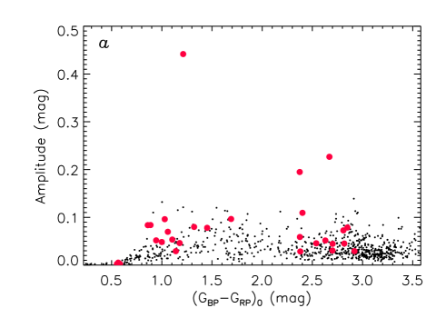
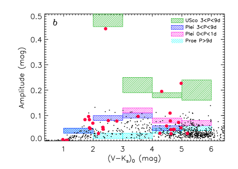
Figure 4: a) Variation amplitudes versus the dereddened colour index $(G_{\rm BP}-G_{\rm RP})_{0}$ for the candidate members of the cluster ASCC 123 (red circles) and for the sample of Pleiades members (small black dots) studied by Rebull et al. (2016). b) Amplitudes as a function of the $(V-K_{\rm s})_{0}$ colour index. The meaning of the symbols is as in panel (a). The hatched rectangles represent the amplitudes at the 80th percentile for the clusters and the period ranges indicated in the legend according to Messina (2021).

One of the main ingredients of dynamo mechanisms generating magnetic fields and operating in stellar interiors is the rotation rate. Therefore, a correlation of magnetic field intensity (or proxies of magnetic field) and the rotation period is expected. Indeed, the correlation with $P_{\rm rot}$ has been widely documented in the literature for several diagnostics of magnetic activity at chromospheric and coronal levels (see, e.g., Cardini & Cassatella, 2007; Frasca et al., 2016; Pizzolato et al., 2003; Reiners et al., 2014). As regards the photospheric activity, traced, e.g., by the variation amplitude, correlation with $P_{\rm rot}$ has been found by Reinhold & Hekker (2020), who subdivided their very large sample of stars with periods and amplitudes detected from $Kepler$-K2 light curves in several subsamples with 200 K temperature bins. They found a general decrease of variability with increasing rotation period for all temperature bins, although the data show large scatter. We plot the variation amplitude as a function of $P_{\rm rot}$ in Fig. 5a. No clear decrease of the amplitude with increasing $P_{\rm rot}$ is visible either for ASCC 123 or the Pleiades. This result is supported by the low Spearman’s correlation coefficient, both for the Pleiades ($\rho\simeq-0.02$) and ASCC 123 ($\rho\simeq+0.12$, even excluding the discrepant star with $P_{\rm rot}=13.4$ days). However, we note that our data include stars with very different $T_{\rm eff}$ values (and consequently different internal structure). As pointed out in several works, including some of those mentioned above, a better variable related to the dynamo action is the Rossby number, $R_{\rm O}=P_{\rm rot}/\tau_{\rm c}$, defined as the ratio of the rotation period and the convective turnover time $\tau_{\rm c}$. The latter is not a directly measurable variable, but can be derived from theoretical models for MS stars or from calibrations as a function of temperature or colour indices. In our case, we have used the empirical relation proposed by Wright et al. (2011, Eq. 10) as a function of $V-K_{S}$. Some correlation, albeit with large scatter, is found between amplitude and $R_{\rm O}$ (Fig. 5b), with Spearman’s coefficients $\rho\simeq-0.16$ and $-0.13$ for ASCC 123 and the Pleiades, respectively.

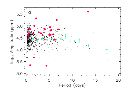
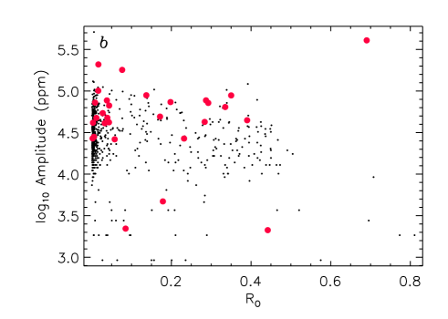
Figure 5: a) Variation amplitudes versus the rotation period for the candidate members of the cluster ASCC 123 (red circles). Small black dots denote the amplitudes for the Pleiades members by Rebull et al. (2016). The green dots and errorbars show the median variability range for the Pleiades for period bins of one day and the standard deviation therein. b) Variation amplitudes versus the Rossby number $R_{\rm O}=P_{\rm rot}/\tau_{\rm c}$.

4.3 Stellar spins orientation

For the stars studied in Paper I, for which we measured accurate values of $v\sin i$, and thanks to the rotational periods, $P_{\rm rot}$, and stellar radii, $R_{*}$, which are reported in Table 1, we can derive the inclination of the rotation axis as:

$$\sin i=\frac{v\sin i}{2\pi R_{*}}P_{\rm rot}.$$ (2)

We found a value of $\sin i<1$ for all the stars, with the exception of S 39. For it, the peak at 1.67 days is marginally consistent (considering the errors) with the value of $v\sin i$ $\simeq\,$49 km s^-1 measured in Paper I, implying an inclination close to 90°, but the TESS light curve phased with this period does not show any clear rotational modulation. We therefore consider this period an uncertain value. However, if the spin axis is nearly parallel to the orbital axis of the presumed transiting object, the inclination of the rotation axis should be very close to 90°, making 1.67 days a possible rotation period for this star. The values of inclination of the rotation axis for the seven stars with HARPS-N spectra are also listed in Table 1.

The statistical sample is too small to study the distribution of the inclinations of the stellar spins and investigate their degree of alignment, as pointed out, e.g., by Corsaro et al. (2017), whose simulations show that a sample 2–3 times larger is required for obtaining a high significance of any eventual spin alignment. However, we wanted to compare the values of $i$ that we find for the seven stars in Table1 with those expected from a random 3D distribution of the rotation axes, in a similar way to what Corsaro et al. (2017) did for giant stars in the old open clusters NGC 6791 and NGC 6819. In their case, for both clusters the $i$ distribution was concentrated towards low values, i.e. it was very different from that expected from a random distribution of the rotation axes (see Figure 1 in their paper), suggesting a significant alignment of the stellar spins. In our case (Fig. 6), the values of inclination are all greater than 50 degrees and are compatible with a random distribution or, in any case, they do not allow us to draw firm conclusions. High- or medium-resolution spectra for a significant number of cluster members, as expected from future multi-object surveys like WEAVE (Jin et al., 2022), are needed to better investigate this aspect. We note that Healy et al. (2021) find that isotropic spins or moderate alignment are both consistent with the $\sin i$ values they derived for members of Pleiades and Praesepe clusters. In a recent work (Healy et al., 2023) found eight out of the ten investigated clusters having spin-axis orientations consistent with isotropy and two clusters whose distributions can be better described by an aligned fraction of stars combined with an isotropic distribution. However, they suggest this result can be influenced by systematic errors on $i$ and by the poor statistics.

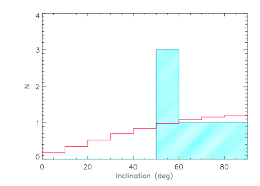
Figure 6: Distribution of the inclination of the rotation axis for the seven stars in Table 1 (light-blue histogram). The red histogram shows the expected distribution for a three-dimensional uniform orientation of the spin vectors.

4.4 Chromospheric activity

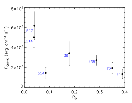
Figure 7: Line flux in the Ca ii-K line as a function of the Rossby number.

Correlations between diagnostics of chromospheric activity and $P_{\rm rot}$, or the Rossby number, have often been reported in the literature (e.g., Douglas et al., 2014; Frasca et al., 2016; Han et al., 2023, and references therein). For rapidly rotating stars, a saturated regime, in which the activity level is constant with $P_{\rm rot}$, is clearly shown by the coronal X-ray emission (e.g. Pizzolato et al., 2003; Wright et al., 2011) but it is also seen at chromospheric level (e.g., Douglas et al., 2014; Newton et al., 2017). In particular, Douglas et al. (2014) found that H$\alpha$ activity is saturated for $R_{\rm O}<0.11$ for members of Hyades and Praesepe, while Newton et al. (2017) found saturation in their sample of nearby field M-type stars for $R_{\rm O}<0.2$.

Despite the small number of stars with measured H$\alpha$ and Ca ii fluxes, we wanted to see if there is any hint of a correlation with rotation in our data. As an example we show $F_{\rm CaII-K}$ as a function of $R_{\rm O}$ in Fig. 7, which clearly shows the decline of flux with increasing $R_{\rm O}$. The only discrepant point is that of the hottest star, S 554. Similar results are also obtained with Ca ii-H and H$\alpha$ as evidenced by the Pearson’s correlation coefficients $\rho=-0.65$, $-0.71$, and $-0.74$, for the H$\alpha$, Ca ii-K, and H line, respectively. Apart from the two F4V sources (S 39 and S 554), only the two ultrafast G-type stars (S 214 and S 517) should have a saturated chromospheric emission, on the basis of their Rossby number. These are the only stars in Table 1 for which a value of X-ray flux is reported in the literature. The values of $F_{\rm X}=3.36\times 10^{-13}$ and $3.65\times 10^{-13}$ erg  cm^-2s^-1 reported by Freund et al. (2022) translate, with the Gaia parallaxes and our values of $T_{\rm eff}$ and $R_{*}$ (Table 1), into $\log(L_{\rm X}/L_{\rm bol})$ values of $-3.36$ and $-3.31$ for S 214 and S 517, respectively. These values are close to the saturation level of $-3.13$ reported by Wright et al. (2011).

To further investigate the behaviour of the magnetic activity at chromospheric level we have compared the different diagnostics by means of flux–flux diagrams. These diagrams are shown, in a logarithm scale, in Fig. 8 along with the power-law relationships found by Martínez-Arnáiz et al. (2011) from their large sample of active FGKM stars. We note that all the members lie, within the error bars, over the flux–flux relation for the Ca ii-K versus Ca ii-H, while the H$\alpha$ fluxes, which are displayed versus Ca ii-K ones in the right panel of Fig. 8, are more scattered. This is consistent with the results of Martínez-Arnáiz et al. (2011), who found a larger scatter in the H$\alpha$–Ca ii flux diagrams compared to diagrams based on different Ca ii lines. Furthermore, they distinguished two different regimes in the H$\alpha$–Ca ii flux diagrams, with the very active late-K and M-type stars significantly deviating from the main behaviour and lying in an upper branch. They argued that these are stars with a saturated X-ray flux. The stars in our sample are all earlier than those in the upper branch of the flux–flux diagrams of Martínez-Arnáiz et al. (2011) and only the ultrafast G-type stars S 214 and S 527 display an activity level close to saturation. The remaining GK-type stars should not be saturated, on the basis of their Rossby number and the above mentioned correlations. However, we note that the two K-type stars F1 and F2 lie right on the average power-law relation (red dotted line in Fig. 8), while the remaining stars are placed systematically lower, but are closer to the lower branch fit (blue dashed line in Fig. 8). The latter was calculated by Martínez-Arnáiz et al. (2011) by excluding the stars with saturated X-ray and H$\alpha$ emission from the fit.

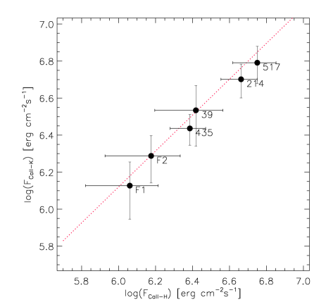
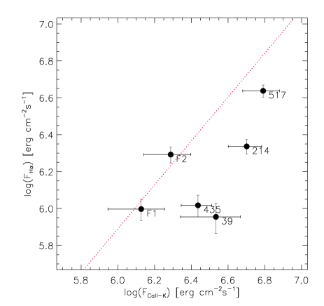
Figure 8: Flux–flux relationships between H & K calcium lines (left panel) and H$\alpha$ (right panel). The red dotted lines represent the power laws that are best fitting the data of Martínez-Arnáiz et al. (2011). The blue dashed-line in the right panel represents the fit to the lower branch of the Martínez-Arnáiz et al. (2011) H$\alpha$ data.

5 Summary and conclusions

In this work we have revisited ASCC 123. It is a little-studied young cluster, with no detailed spectroscopic investigation apart our recent study (Frasca et al., 2019). In that paper we determined the main properties of the cluster such as distance, age and chemical composition by combining $Gaia$ data with high-resolution spectroscopy taken with HARPS-N at the TNG telescope. In the present work we have focused on rotation and magnetic activity. With this aim we retrieved TESS photometry for all the 55 cluster members reported in Cantat-Gaudin et al. (2018). Among them, seven FGK-type stars were observed spectroscopically in our previous work. We performed the analysis of the light curves of the cluster members obtaining the rotational periods and amplitudes for 29 objects. By comparing the distributions of period and amplitude versus colour index with those of some well-studied clusters, we infer a gyrochronogical age for ASCC 123 similar to that of the Pleiades, which is consistent with our precedent estimates based on the isochrone fitting and abundance of lithium. No clear correlation between the variation amplitude and $P_{\rm rot}$ is observed, while a Spearman’s coefficient $\rho=-0.16$ between amplitude and Rossby number suggests only a marginal correlation of these variables. Additionally, for the seven stars with spectra we have derived the inclination of the rotational axis. Although our sample is not statistically significant, the distribution of inclinations seems to be random, which would be in agreement with that observed in other young open clusters. Finally, we studied the level of magnetic activity of these stars from the H$\alpha$ and Ca ii H&K lines. We find that the chromospheric activity indicators display a better correlation with the Rossby number ($\rho$ in the range [$-0.65,-0.74$]). Moreover, they follow the general trends observed in other active FGKM stars in the flux–flux diagrams.

Data Availability

The spectroscopic and ground-based photometric data underlying this paper will be shared on reasonable request to the corresponding author. TESS photometric data are available at https://archive.st sci.edu/.

Appendix A Ground-based photometry

As mentioned in Sect. 2.2, we collected multiband $BVR_{\rm C}I_{\rm C}$ photometry of the three G-type stars S 214, S 435, and S 517 at OACT. Despite the lower photometric precision, compared with TESS data, and the irregular sampling of our photometry, we were able to detect the rotational modulation and derive the period for the two ultrafast rotators (S 214 and S 517). The light curves in the $BVR_{\rm C}I_{\rm C}$ bands of S 214 are shown in Fig. 9. The peak at a rotation period of 0.564 days is the highest one in the cleaned power spectrum of each band and is also recovered from the TESS photometry of this source (see Sect. 3.1). The amplitudes of the $BVR_{\rm C}I_{\rm C}$ light curves are about 0.11, 0.15, 0.08, and 0.07 mag, respectively. The average magnitudes of these stars in the Johnson-Cousins bands from our OACT photometry are listed in Table 4.

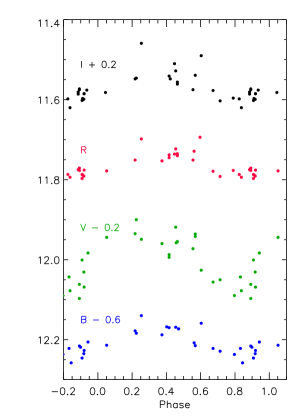
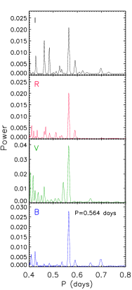
Figure 9: (Left panel) Phased $BVR_{\rm C}I_{\rm C}$ light curves of S 214 collected at OACT. (Right panels) Cleaned periodograms.

Table 4: Mean Johnson-Cousins magnitudes of the three G-type members observed at OACT.

ID	$B$	err	$V$	err	$R_{\rm C}$	err	$I_{\rm C}$	err
	(mag)		(mag)		(mag)		(mag)
214	12.866	0.031	12.192	0.051	11.769	0.026	11.403	0.022
435	12.993	0.033	12.242	0.035	11.922	0.033	11.527	0.029
517	13.093	0.028	12.199	0.036	11.773	0.025	11.417	0.022

Appendix B Additional figures

Figure 11: Zoom of the two transits detected in the TESS light curve of S 39 (TIC 64837857) in sectors 16 (upper panel) and 17 (lower panel).

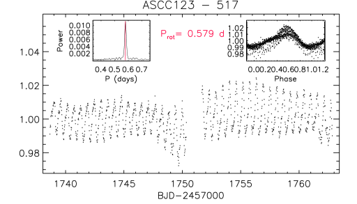
Figure 12: TESS light curve of S 517 (TIC 428274538) in 2019 (Sector 16). The inset in the upper left corner shows the cleaned periodogram of these data; the rotation period is marked with a vertical red line. The inset in the upper right corner displays the data phased with this period.

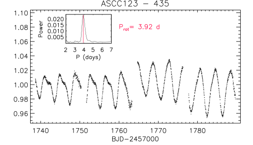
Figure 14: TESS light curve of S 435 (TIC 388696341) in 2019 (sectors 16 and 17). The inset in the upper left corner shows the cleaned periodogram of these data; the rotation period is marked with a vertical red line.

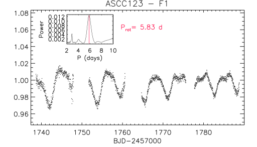
Figure 15: TESS light curve of F1 (TIC 66539637) in 2019 (sectors 16 and 17). The figure layout is the same as Fig. 14.

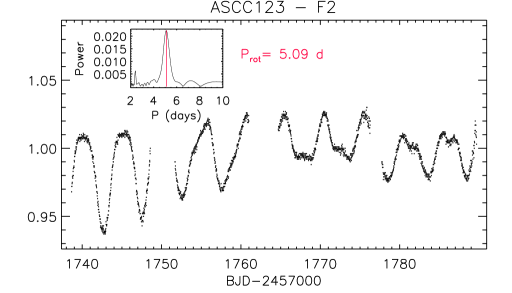
Figure 16: TESS light curve of F2 (TIC 64077901) in 2019 (sectors 16 and 17). The figure layout is the same as Fig. 14.

References

- Allard et al. (2012) Allard F., Homeier D., Freytag B., 2012, Philosophical Transactions of the Royal Society of London Series A, 370, 2765
- Altmann et al. (2017) Altmann M., Roeser S., Demleitner M., Bastian U., Schilbach E., 2017, A&A, 600, L4
- Barnes (2003) Barnes S. A., 2003, ApJ, 586, 464
- Barnes et al. (2015) Barnes S. A., Weingrill J., Granzer T., Spada F., Strassmeier K. G., 2015, A&A, 583, A73
- Barnes et al. (2016) Barnes S. A., Spada F., Weingrill J., 2016, Astronomische Nachrichten, 337, 810
- Barry et al. (1987) Barry D. C., Cromwell R. H., Hege E. K., 1987, ApJ, 315, 264
- Bossini et al. (2019) Bossini D., et al., 2019, A&A, 623, A108
- Bressan et al. (2012) Bressan A., Marigo P., Girardi L., Salasnich B., Dal Cero C., Rubele S., Nanni A., 2012, MNRAS, 427, 127
- Cantat-Gaudin et al. (2018) Cantat-Gaudin T., et al., 2018, A&A, 618, A93
- Cantat-Gaudin et al. (2020) Cantat-Gaudin T., et al., 2020, A&A, 640, A1
- Cardini & Cassatella (2007) Cardini D., Cassatella A., 2007, ApJ, 666, 393
- Claudi et al. (2017) Claudi R., et al., 2017, European Physical Journal Plus, 132, 364
- Corsaro et al. (2017) Corsaro E., et al., 2017, Nature Astronomy, 1, 0064
- Douglas et al. (2014) Douglas S. T., et al., 2014, ApJ, 795, 161
- Feiden (2016) Feiden G. A., 2016, A&A, 593, A99
- Frasca & Catalano (1994) Frasca A., Catalano S., 1994, A&A, 284, 883
- Frasca et al. (2010) Frasca A., Biazzo K., Kővári Z., Marilli E., Çakırlı Ö., 2010, A&A, 518, A48
- Frasca et al. (2016) Frasca A., et al., 2016, A&A, 594, A39
- Frasca et al. (2019) Frasca A., et al., 2019, A&A, 632, A16 (Paper I)
- Freund et al. (2022) Freund S., Czesla S., Robrade J., Schneider P. C., Schmitt J. H. M. M., 2022, A&A, 664, A105
- Fritzewski et al. (2021) Fritzewski D. J., Barnes S. A., James D. J., Strassmeier K. G., 2021, A&A, 652, A60
- Gaia Collaboration (2022) Gaia Collaboration 2022, VizieR Online Data Catalog, p. I/355
- Gutiérrez Albarrán et al. (2020) Gutiérrez Albarrán M. L., et al., 2020, A&A, 643, A71
- Han et al. (2023) Han H., Wang S., Bai Y., Yang H., Fang X., Liu J., 2023, ApJS, 264, 12
- Healy et al. (2021) Healy B. F., McCullough P. R., Schlaufman K. C., 2021, ApJ, 923, 23
- Healy et al. (2023) Healy B. F., McCullough P. R., Schlaufman K. C., Kovacs G., 2023, ApJ, 944, 39
- Huang et al. (2020) Huang C. X., et al., 2020, Research Notes of the American Astronomical Society, 4, 204
- Ianna & Schlemmer (1993) Ianna P. A., Schlemmer D. M., 1993, AJ, 105, 209
- Jeffries (2014) Jeffries R. D., 2014, in EAS Publications Series. pp 289–325 (arXiv:1404.7156), doi:10.1051/eas/1465008
- Jin et al. (2022) Jin S., et al., 2022, arXiv e-prints, p. arXiv:2212.03981
- Kharchenko et al. (2005) Kharchenko N. V., Piskunov A. E., Röser S., Schilbach E., Scholz R. D., 2005, A&A, 440, 403
- Martínez-Arnáiz et al. (2011) Martínez-Arnáiz R., López-Santiago J., Crespo-Chacón I., Montes D., 2011, MNRAS, 414, 2629
- Messina (2021) Messina S., 2021, A&A, 645, A144
- Nardiello et al. (2019) Nardiello D., et al., 2019, MNRAS, 490, 3806
- Newton et al. (2017) Newton E. R., Irwin J., Charbonneau D., Berlind P., Calkins M. L., Mink J., 2017, ApJ, 834, 85
- Paegert et al. (2022) Paegert M., Stassun K. G., Collins K. A., Pepper J., Torres G., Jenkins J., Twicken J. D., Latham D. W., 2022, VizieR Online Data Catalog, p. IV/39
- Pizzolato et al. (2003) Pizzolato N., Maggio A., Micela G., Sciortino S., Ventura P., 2003, A&A, 397, 147
- Rebull et al. (2016) Rebull L. M., et al., 2016, AJ, 152, 113
- Rebull et al. (2022) Rebull L. M., Stauffer J. R., Hillenbrand L. A., Cody A. M., Kruse E., Powell B. P., 2022, AJ, 164, 80
- Reiners et al. (2014) Reiners A., Schüssler M., Passegger V. M., 2014, ApJ, 794, 144
- Reinhold & Hekker (2020) Reinhold T., Hekker S., 2020, A&A, 635, A43
- Ricker et al. (2015) Ricker G. R., et al., 2015, Journal of Astronomical Telescopes, Instruments, and Systems, 1, 014003
- Roberts et al. (1987) Roberts D. H., Lehar J., Dreher J. W., 1987, AJ, 93, 968
- Scargle (1982) Scargle J. D., 1982, ApJ, 263, 835
- See et al. (2021) See V., Roquette J., Amard L., Matt S. P., 2021, ApJ, 912, 127
- Skrutskie et al. (2006) Skrutskie M. F., et al., 2006, AJ, 131, 1163
- Skumanich (1972) Skumanich A., 1972, ApJ, 171, 565
- Soderblom et al. (1991) Soderblom D. R., Duncan D. K., Johnson D. R. H., 1991, ApJ, 375, 722
- Spada & Lanzafame (2020) Spada F., Lanzafame A. C., 2020, A&A, 636, A76
- Stanford-Moore et al. (2020) Stanford-Moore S. A., Nielsen E. L., De Rosa R. J., Macintosh B., Czekala I., 2020, ApJ, 898, 27
- Stassun et al. (2019) Stassun K. G., et al., 2019, AJ, 158, 138
- Stetson (2000) Stetson P. B., 2000, PASP, 112, 925
- Wang & Chen (2019) Wang S., Chen X., 2019, ApJ, 877, 116
- Wright et al. (2011) Wright N. J., Drake J. J., Mamajek E. E., Henry G. W., 2011, ApJ, 743, 48
- Yen et al. (2018) Yen S. X., Reffert S., Schilbach E., Röser S., Kharchenko N. V., Piskunov A. E., 2018, A&A, 615, A12