Helmholtz FEM solutions are locally quasi-optimal modulo low frequencies

Abstract

For $h$-FEM discretisations of the Helmholtz equation with wavenumber $k$, we obtain $k$-explicit analogues of the classic local FEM error bounds of [25], [28, §9], [8], showing that these bounds hold with constants independent of $k$, provided one works in Sobolev norms weighted with $k$ in the natural way.

We prove two main results: (i) a bound on the local $H^{1}$ error by the best approximation error plus the $L^{2}$ error, both on a slightly larger set, and (ii) the bound in (i) but now with the $L^{2}$ error replaced by the error in a negative Sobolev norm. The result (i) is valid for shape-regular triangulations, and is the $k$-explicit analogue of the main result of [8]. The result (ii) is valid when the mesh is locally quasi-uniform on the scale of the wavelength (i.e., on the scale of $k^{-1}$) and is the $k$-explicit analogue of the results of [25], [28, §9].

Since our Sobolev spaces are weighted with $k$ in the natural way, the result (ii) indicates that the Helmholtz FEM solution is locally quasi-optimal modulo low frequencies (i.e., frequencies $\lesssim k$). Numerical experiments confirm this property, and also highlight interesting propagation phenomena in the Helmholtz FEM error.

AMS subject classifications: 35J05, 65N15, 65N30, 78A45

1 Introduction: the main result in a simple setting

1.1 The PML approximation to the Helmholtz exterior Dirichlet problem and its FEM discretisation.

Let $\Omega_{-}\subset\mathbb{R}^{d}$ be a bounded Lipschitz open set with its open complement $\Omega_{+}:=\mathbb{R}^{d}\setminus\overline{\Omega_{-}}$ connected. Let $\widetilde{u}$ be the solution of the variable coefficient exterior Dirichlet problem for the Helmholtz equation

$$-k^{-2}\nabla\cdot\big{(}A_{\rm scat}(x)\nabla\widetilde{u}(x)\big{)}-(c_{\rm scat}(x))^{-2}\widetilde{u}(x)=g(x)\quad\textup{in }\Omega_{+},\qquad\widetilde{u}=0\quad\text{ on }\partial\Omega_{+}$$

satisfying the Sommerfeld radiation condition, and with the supports of $g$, $I-A_{\rm scat}$, and $1-c_{\rm scat}$ compact. Let $u\in H^{1}_{0}(\Omega)$ be the radial perfectly-matched-layer (PML) approximation to $\widetilde{u}$, where $\Omega$ is the truncated domain; i.e., $u$ is the solution to the variational problem

$$\textup{find }u\in H^{1}_{0}(\Omega)\textup{ such that }a(u,v)=G(v)\text{ for all }v\in H^{1}_{0}(\Omega),$$ (1.1)

where $a$ is the sesquilinear form given by

$$a(u,v)=\int_{\Omega}k^{-2}A\nabla u\cdot\overline{\nabla v}-c^{-2}u\overline{v}\,,$$

$G(v)=\int_{\Omega}g\overline{v}$, and the coefficients $A$ and $c$ are defined in §7.1.5 in terms of the PML scaling function and (respectively) $A_{\rm scat}$ and $c_{\rm scat}$.

We consider the Galerkin discretisation of (1.1) using the standard conforming Lagrange finite element spaces $\{V_{h}\}_{h>0}$ of continuous piecewise polynomials of degree $p$ on a family of shape-regular triangulations $(\mathcal{T}_{h})_{h>0}$ of $\Omega$; i.e.,

$$\textup{find }u_{h}\in V_{h}\textup{ such that }a(u_{h},v_{h})=G(v_{h})\quad\text{ for all }v_{h}\in V_{h}.$$ (1.2)

Subtracting (1.2) from (1.1) we find that Galerkin orthogonality holds:

$$a(u-u_{h},v_{h})=0\quad\text{ for all }v_{h}\in V_{h}.$$ (1.3)

1.2 First result: bound on the local FEM error in $H^{1}_{k}$ with an $L^{2}$ error term.

Given two subsets $A\subset B\subset\Omega$, let

$$\partial_{<}(A,B):=\textup{dist}\big{(}\partial A\setminus\partial\Omega,\partial B\setminus\partial\Omega\big{)},$$ (1.4)

with the convention $\partial_{<}(A,B)=+\infty$ when $B=\Omega$. Working with this notion of distance allows us to consider subdomains that go up to the boundary.

The Sobolev norms $\|\cdot\|_{H^{s}_{k}(D)}$ for $D$ a bounded Lipschitz domain are defined as for $\|\cdot\|_{H^{s}(D)}$ (via restriction of $\|\cdot\|_{H^{s}(\mathbb{R}^{d})}$ to $D$, with this second norm defined by the Fourier transform), except that now we weight the $j$th derivative with $k^{-j}$; see §A.

Theorem 1.1 (Local quasioptimality in $H^{1}_{k}$ up to an $L^{2}$ error term)

Suppose that $A$ and $c$ are $L^{\infty}(\Omega)$ and the PML scaling function $f_{\theta}$ (defined in §7.1.5) is $W^{1,\infty}(\Omega)$. Given $C_{0}>0$ there exists $C_{1},C_{*}>0$ such that the following is true. Let $\Omega_{0}\subset\Omega_{1}\subset\Omega$ be such that $\Omega_{0}\neq\Omega_{1}$,

$$d:=\partial_{<}(\Omega_{0},\Omega_{1})\geq\frac{C_{0}}{k},\quad\text{ and }\quad\max_{K\cap\Omega_{1}\neq\emptyset}h_{K}\leq\frac{C_{1}}{k}.$$ (1.5)

Given $k>0$, let $u\in H^{1}_{0}(\Omega)$ and $u_{h}\in V_{h}$ satisfy the Galerkin orthogonality (1.3). Then

$${\left\lVert{u-u_{h}}\right\rVert}_{H^{1}_{k}(\Omega_{0})}\leq C_{*}\Big{(}\min_{w_{h}\in V_{h}}{\left\lVert{u-w_{h}}\right\rVert}_{H^{1}_{k}(\Omega_{1})}+{\left\lVert{u-u_{h}}\right\rVert}_{L^{2}(\Omega_{1})}\Big{)}.$$ (1.6)

We make two remarks (which also hold for Theorem 1.2 below).

1. Recall that, for standard finite-element spaces with $p$ fixed, $h_{K}k$ must be chosen as a decreasing function of $k$ to maintain accuracy (see [13] and the references therein); thus the second condition in (1.5) is not restrictive.

2. The assumption that $u$ and $u_{h}$ satisfy the Galerkin orthogonality (1.3) can be weakened to $u$ and $u_{h}$ satisfying a local version of Galerkin orthogonality on $\Omega_{1}$; see (4.2) below.

1.3 Second result: bound on the local FEM error in $H^{1}_{k}$ with an error term in a negative norm

Theorem 1.1 holds for all shape-regular meshes $\mathcal{T}_{h}$ (i.e., the mesh elements are uniformly “well-shaped”), and thus the mesh can in principle be highly non-uniform. However, if the mesh $\mathcal{T}_{h}$ is locally quasi-uniform on a scale of $k^{-1}$ (i.e., in every ball of radius proportional to $k^{-1}$, the mesh elements diameters are comparable), then the $L^{2}$ norm of the error on the right-hand side of (1.6) can be replaced by a negative Sobolev norm.

Theorem 1.2 (Local quasioptimality in $H^{1}_{k}$ up to an error term in a negative norm)

Suppose that, for some $\ell\in\mathbb{Z}^{+}$, $A$ and $c$ are $C^{\ell,1}(\Omega)$, the PML scaling function $f_{\theta}$ (defined in §7.1.5) is $C^{\ell+1,1}(\Omega)$, and $\partial\Omega$ is $C^{\ell+1,1}$. Given $C_{0},C_{\rm qu}>0$ there exists $C_{1},C_{2},C_{*}>0$ such that the following is true. Let $\Omega_{0}\subset\Omega_{1}\subset\Omega$ be such that $\Omega_{0}\neq\Omega_{1}$ and (1.5) holds. Assume further that $\mathcal{T}$ is quasi-uniform on scale $k^{-1}$, in the sense that, for every ball $B$ of radius at most $C_{2}k^{-1}$,

$$\frac{\max_{K\cap B\neq\emptyset}h_{K}}{\min_{K\cap B\neq\emptyset}h_{K}}\leq C_{\rm qu}.$$ (1.7)

Given $k>0$, let $u\in H^{1}_{0}(\Omega)$ and $u_{h}\in V_{h}$ satisfy (1.3). Then

$${\left\lVert{u-u_{h}}\right\rVert}_{H^{1}_{k}(\Omega_{0})}\leq C_{*}\Big{(}\min_{w_{h}\in V_{h}}{\left\lVert{u-w_{h}}\right\rVert}_{H^{1}_{k}(\Omega_{1})}+{\left\lVert{u-u_{h}}\right\rVert}_{(H_{k}^{\min\{\ell+1,p\},<}(\Omega_{1}))^{*}}\Big{)}.$$ (1.8)

Note that meshes satisfying (1.7) can be highly non-uniform on $\Omega$; indeed, the ratio between the largest and smallest mesh elements on an ${\cal O}(1)$ scale can be proportional to $\exp(\alpha k)$ for some $\alpha\in\mathbb{R}$ (depending on $C_{\rm qu}$).

We now define the norm ${\left\lVert{\cdot}\right\rVert}_{(H_{k}^{s,<}(\Omega_{1}))^{*}}$ appearing in the last term on the right-hand side of (1.8), but highlight that when $\Omega_{1}$ is an interior subset of $\Omega$, ${\left\lVert{\cdot}\right\rVert}_{(H_{k}^{s,<}(\Omega_{1}))^{*}}$ is equivalent to $\|\cdot\|_{H_{k}^{-s}(\Omega_{1})}$. For $s\geq 0$ and $D\subset\Omega$ Lipschitz, let

$$H^{s,<}(D):=\overline{\Big{\{}v\in H^{s}(D)\cap H^{1}_{0}(\Omega):{\rm supp}\,v\subset\overline{D},\,\partial_{<}({\rm supp}\,v,D)>0\Big{\}}}$$

(where the closure is taken with respect to the $H^{s}$ norm) and

$${\left\lVert{v}\right\rVert}_{(H_{k}^{s,<}(D))^{*}}:=\sup_{w\in H^{s,<}(D),\,\|w\|_{H^{s}(D)}=1}\big{|}\langle v,w\rangle_{D}\big{|}.$$

When $\partial D\cap\partial\Omega=\emptyset$ (i.e., $D$ is an interior subset of $\Omega$), ${\left\lVert{\cdot}\right\rVert}_{(H_{k}^{s,<}(D))^{*}}$ is equivalent to $\|\cdot\|_{H_{k}^{-s}(D)}$ by (A.4) (see also [28, Equation 9.18]). When $\partial D\cap\partial\Omega\neq\emptyset$,

$$H_{0}^{s}(D)\subset H^{s,<}(D)\subset H^{s}(D)\cap H^{1}_{0}(D)$$

(where $H_{0}^{s}(D)$ is the closure of $C^{\infty}_{\rm comp}(D)$ in $H^{s}(D)$), and so

$$\left\|v\right\|_{H^{-s}_{k}(D)}\leq{\left\lVert{v}\right\rVert}_{(H_{k}^{s,<}(D))^{*}}\leq C\max\big{\{}\left\|v\right\|_{H^{-1}_{k}(D)},\left\|v\right\|_{\widetilde{H}^{-s}_{k}(D)}\big{\}}.$$

To informally understand the differences between these norms, we note that $\left\|\cdot\right\|_{H^{-s}_{k}(D)}$ doesn’t “see” the boundary of $D$, $\left\|v\right\|_{\widetilde{H}^{-s}_{k}(D)}$ sees the boundary of $D$, and ${\left\lVert{v}\right\rVert}_{(H_{k}^{s,<}(D))^{*}}$ sees only the parts of $\partial D$ that coincide with $\partial\Omega$.

1.4 The relationship of Theorems 1.1 and 1.2 to other results in the literature.

Estimates on the local FEM error for second-order linear elliptic PDEs were pioneered by Nitsche and Schatz in [25]; see also [9], [26], [27], [28, Chapter 9], and [8]. These arguments use that the sesquilinear forms of second-order linear elliptic PDEs are coercive (i.e., sign definite) on sufficiently-small balls. This property is used to prove, again on small balls, a discrete analogue of the classic Caccioppoli estimate (bounding the $H^{1}$ norm of the PDE solution in terms of the $L^{2}$ norm and the data on a slightly larger set). The Caccioppoli estimate is the main ingredient required to prove a bound of the form (1.6) on small balls. A covering argument is then used to obtain the bound on an arbitrary domain from the bound on small balls. These arguments combined with a duality argument and elliptic regularity then produce a bound of the form (1.8).

Although these classic results apply to the Helmholtz equation, they don’t use norms weighted with $k$ and the constants in the bounds are not explicit in $k$. The main motivation for the present paper was to obtain the analogues of the results in [25], [28, Chapter 9], and [8] applied to the Helmholtz equation in $k$-weighted norms, and with constants explicit in $k$. Roughly speaking, we show that the results of [25], [28, Chapter 9], and [8] hold for the Helmholtz equation with constants independent of $k$, provided that one works in $k$-weighted norms. In more detail,

• Theorem 1.1 is a $k$-explicit version of [8, Theorem 3.4], with both proved under the assumption that the mesh is shape-regular. This result (in non $k$-explicit form) for quasi-uniform meshes appears as [9, Theorem 4], [27, Theorem 4.1], and [28, Theorem 9.1].

• Theorem 1.2 is, roughly-speaking, a $k$-explicit version of [25, Theorem 5.1(i)] and [28, Theorem 9.2]. The differences are

  • in [25, Theorem 5.1(i)] the best approximation error on $\Omega_{1}$ (i.e., the first term on the right-hand sides of (1.6) and (1.8)) is estimated by the standard polynomial approximation result ((3.22) below) and the subdomains are assumed not to touch the boundary, and

  • the results in [25] and [28, Chapter 9] are geared towards quasi-uniform meshes (see [25, Assumption A3], [28, Equation 9.6]) whereas Theorem 1.2 requires quasi-uniformity only on the scale of the wavelength (i.e., on a scale of $k^{-1}$).

An additional difference between the results of the present paper and existing results is that we cover Helmholtz transmission problems, i.e., those with discontinuous $A_{\rm scat}$ and $c_{\rm scat}$, and Theorem 1.2 in this context appears to be new (independent of the $k$-explicitness); indeed, [25, 9] consider second order linear elliptic PDEs with smooth coefficients and [27, 28] cover Poisson’s equation.

1.5 Interpreting the results of Theorems 1.1 and 1.2.

The standard interpretation of the non-$k$-explicit versions of the bounds (1.6) and (1.8) is that the FEM solution is locally quasi-optimal up to a lower-order term that allows error to propagate into $\Omega_{0}$ from the rest of the domain. (This second term is sometimes called the “pollution” or “slush” term in the literature; later in the paper we refer to it as the “slush” term to avoid confusion with the pollution effect for the Helmholtz $h$-FEM.)

The fact that (1.6) and (1.8) are proved in $k$-weighted norms with $k$-independent constants allows this interpretation to be refined in the Helmholtz context to Helmholtz FEM solutions are locally quasi-optimal modulo low frequencies, where “low frequencies” here means “frequencies $\leq Ck$ for some $C>1$”.

We now show (albeit heuristically) how this property can be inferred from the bounds (1.6) (1.8), with this property illustrated by numerical experiments in §2.

The key point is that a bound on a high $k$-weighted Sobolev norm of a function in terms of a low $k$-weighted Sobolev norm, with the constant independent of $k$, implies that the function is controlled by its frequencies $\lesssim k$. This is illustrated by the following simple lemma.

Lemma 1.3

(Bound on high Sobolev norm by low Sobolev norm implies function controlled by its low frequencies) Suppose a family of functions $(f(k))_{k>0}$ is such that $f(k)\in H^{1}_{k}(\mathbb{R}^{d})$ and there exists $C_{2}>0$ such that given $s>0$ there exists $C_{1}>0$ such that

$$\left\|f\right\|^{2}_{H^{1}_{k}(\mathbb{R}^{d})}\leq C_{1}\Big{(}C_{2}+\left\|f\right\|^{2}_{H^{-s}_{k}(\mathbb{R}^{d})}\Big{)}\text{ for all }k\geq k_{0}.$$ (1.9)

If

$$\frac{C_{1}}{R^{2(s+1)}}\leq\frac{1}{2},$$ (1.10)

then, for all $k\geq k_{0}$,

$$\bigg{(}\frac{k}{2\pi}\bigg{)}^{d}\int_{\mathbb{R}^{d}}\langle\xi\rangle^{2}|\mathcal{F}_{k}f(\xi)|^{2}\,{\rm d}\xi\leq 2C_{1}\Bigg{(}C_{2}+\bigg{(}\frac{k}{2\pi}\bigg{)}^{d}\int_{|\xi|\leq R}\langle\xi\rangle^{-2s}|\mathcal{F}_{k}f(\xi)|^{2}\,{\rm d}\xi\Bigg{)}.$$

In the “ideal” situation that $C_{1}=(C)^{2(s+1)}$, (1.10) can be satisfied by taking $R>C$ and $s$ large; we call this the “ideal” situation, since (1.9) holds with this value of $C_{1}$ (and $C_{2}=0$) when $|\mathcal{F}_{k}f(\xi)|=0$ for $\langle\xi\rangle\geq C$.

Proof of Lemma 1.3. By the definition of $\|\cdot\|_{H^{s}_{k}(\mathbb{R}^{d})}$ (A.2),

$$\int_{\mathbb{R}^{d}}\langle\xi\rangle^{2}|\mathcal{F}_{k}f(\xi)|^{2}\,{\rm d}\xi\leq C_{1}\bigg{(}\bigg{(}\frac{2\pi}{k}\bigg{)}^{d}C_{2}+\int_{|\xi|\leq R}\langle\xi\rangle^{-2s}|\mathcal{F}_{k}f(\xi)|^{2}\,{\rm d}\xi+\frac{1}{R^{2(s+1)}}\int_{|\xi|\geq R}\langle\xi\rangle^{2}|\mathcal{F}_{k}f(\xi)|^{2}\,{\rm d}\xi\bigg{)},$$

and the result follows.   

The bound (1.8) is conceptually similar to the setting of Lemma 1.3 of a high Sobolev norm of $u-u_{h}$ being bounded by one of its low Sobolev norms, except that (i) the norm on the right-hand side is over a slightly larger domain ($\Omega_{1}$ vs $\Omega_{0}$) (ii) the order of the negative norm (i.e., $s$ in (1.9)) cannot be arbitrarily large.

Nevertheless we expect from (1.8) that $u-u_{h}$ is controlled locally by the local best approximation error and the low frequencies of $u-u_{h}$; i.e., the Galerkin solution is locally quasi-optimal, modulo low frequencies.

1.6 Outline of the paper.

Section 2 contains numerical experiments illustrating local quasi-optimality modulo low frequencies of Helmholtz FEM solutions.

Section 3 describes a general framework, with Section 7 then showing how a variety of Helmholtz problems fit in this framework (including the exterior Dirichlet problem and transmission problem discussed above).

Section 4 states the main results applied to the general framework, with Theorem 4.1 the generalisation of Theorem 1.1 and Theorem 4.2 the generalisation of Theorem 1.2

Section 6 proves Theorems 1.1 and 1.2, with Section 5 proving auxiliary results (Caccioppoli estimates) used in the proofs.

The appendix (§A) recaps the definitions of Sobolev spaces weighted by $k$.

2 Numerical experiments illustrating local quasi-optimality modulo low frequencies of Helmholtz FEM solutions

This section presents numerical experiments where the error in the Helmholtz FEM solution behaves differently in different subsets of the domain due to either

1. a non-uniform mesh, see §2.1, or

2. the solution being zero in some part of the domain (so that the local best approximation error is immediately zero in this part of the domain), see §2.2.

These situations are manufactured so that each of the two terms on the right-hand side of (1.8) is dominant in a different subset of the domain.

Our ultimate aim is to study the local behaviour of the FEM error for scattering problems. However, a proper understanding of this situation requires understanding the $k$-dependence of the two terms on the right-hand side of (1.8) as a function of the position of $\Omega_{1}$ relative to the scatterer; this is work in progress and will be reported elsewhere.

In all the experiments, the Galerkin equations (1.2) are formulated with the software FreeFem++ [17] using continuous Lagrange elements of degree $p=1,\ldots,4$. The resulting linear systems are then solved using the parallel domain decomposition toolbox HPDDM. The code used to produce these numerical results is available at https://github.com/MartinAverseng/local_qo_experiments.

In the experiments we compute “low” and “high” frequency components of the FEM error; how we do this is described in §2.3 below, with the “low” and “high” frequencies corresponding to the components of the solution with the absolute value of the Fourier variable $\leq 2k$ and $\geq 2k$, respectively.

2.1 Experiments with a non-uniform mesh

We solve the interior impedance problem in a rectangular domain $\Omega=[0,2.1]\times[0,1]$, i.e.,

$$(k^{-2}\Delta+1)u=0\quad\text{ in }\Omega\quad\text{ and }\quad k^{-1}\partial_{n}u-{\rm i}u=g\quad\text{ on }\partial\Omega,$$

with data $g$ is chosen so that the exact solution is the plane wave $u=\exp\left({\rm i}k(\cos(\theta)x+\sin(\theta)y)\right)$.

This problem falls into the class of Helmholtz problems described in §7.1, with the sesquilinear form given by (7.8) with $A_{\rm scat}=I$, $c_{\rm scat}=1$, $\Omega_{-}=\emptyset$ (no impenetrable obstacle), $\Omega_{\rm p}=\emptyset$ (no penetrable obstacle), and $\Omega_{{\rm tr}}=\Omega$.

Experiment 1.

We consider two different mesh sizes $h_{1}>h_{2}$ and consider the following three different meshes on $\Omega$:

• a globally-uniform mesh of size $h_{1}$,

• a globally-uniform mesh of size $h_{2}$,

• a mesh with sizes $h_{1}$ in the left-hand square $[0,1]\times[0,1]$, $h_{2}$ in the right-hand square $[1.1,2.1]\times[0,1]$, and some non-constant mesh size in the transition region $[1,1.1]\times[0,1]$.

Figure 2.1 shows an example of the third type of mesh.

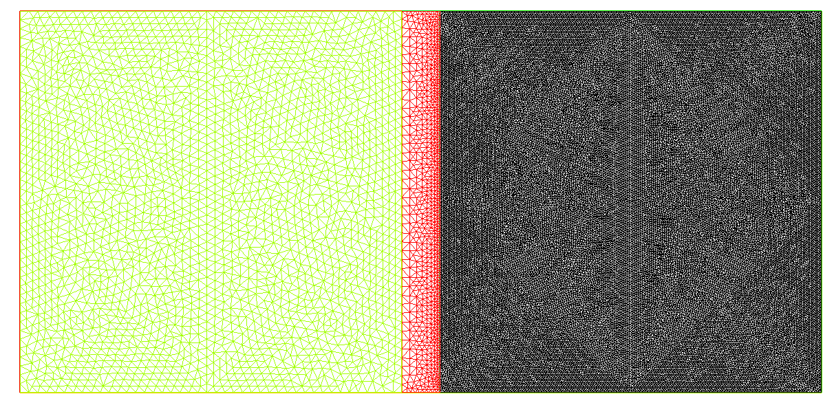
Figure 2.1: A mesh with two square regions $S_{1}$ and $S_{2}$ each with a uniform mesh size (different to each other).

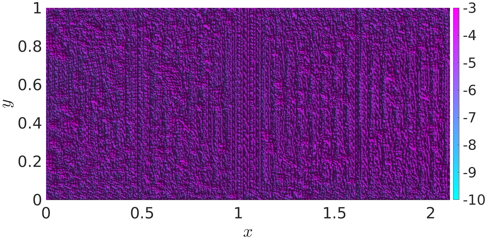
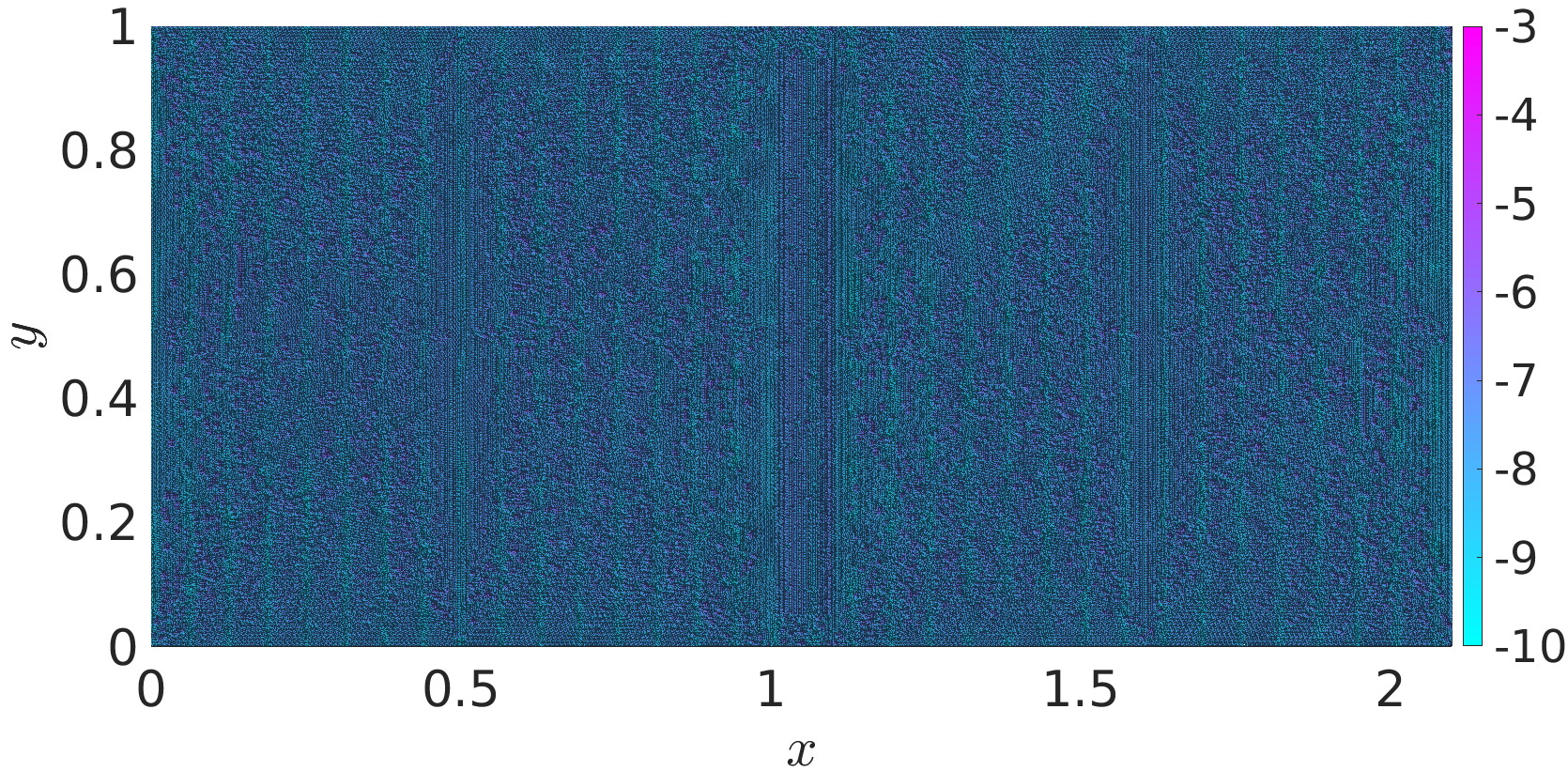
Figure 2.2: For Experiment 1 in §2.1, plot of the quantity $\log(10^{-12}+{\left\lvert{\Re(u-u_{h})}\right\rvert})/\log(10)$, for $k=50$, $p=4$ and $\theta=0$. Top left: globally uniform mesh with $h=1.78k^{-1}$. Top right: globally uniform mesh with $h=0.38k^{-1}$. Bottom: non-uniform mesh, with a coarse region $h_{1}=1.78k^{-1}$ and a fine region with $h_{2}=0.38k^{-1}$.

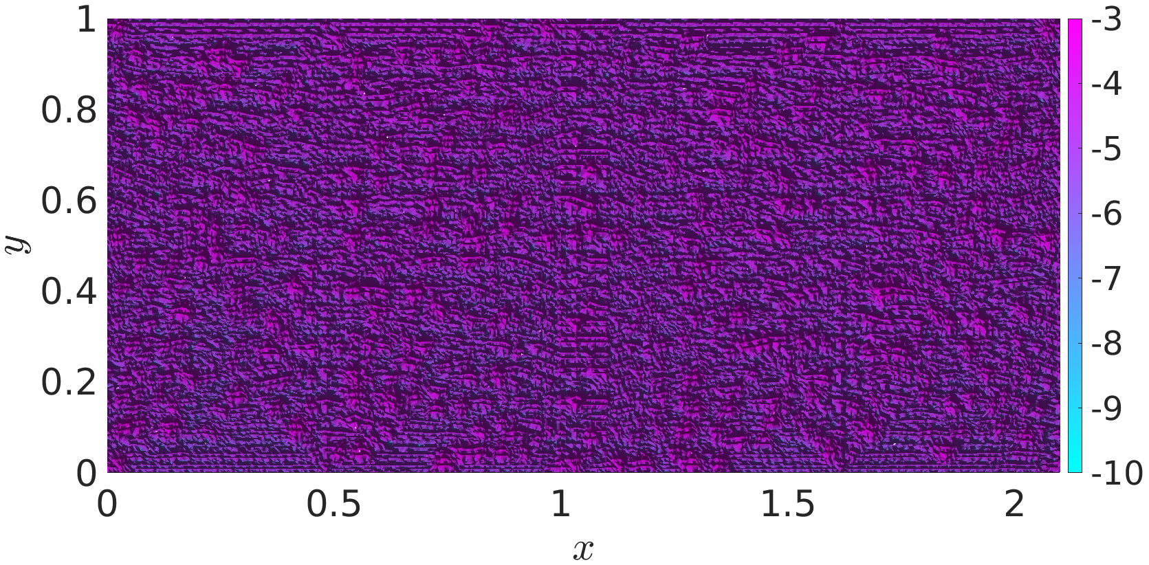
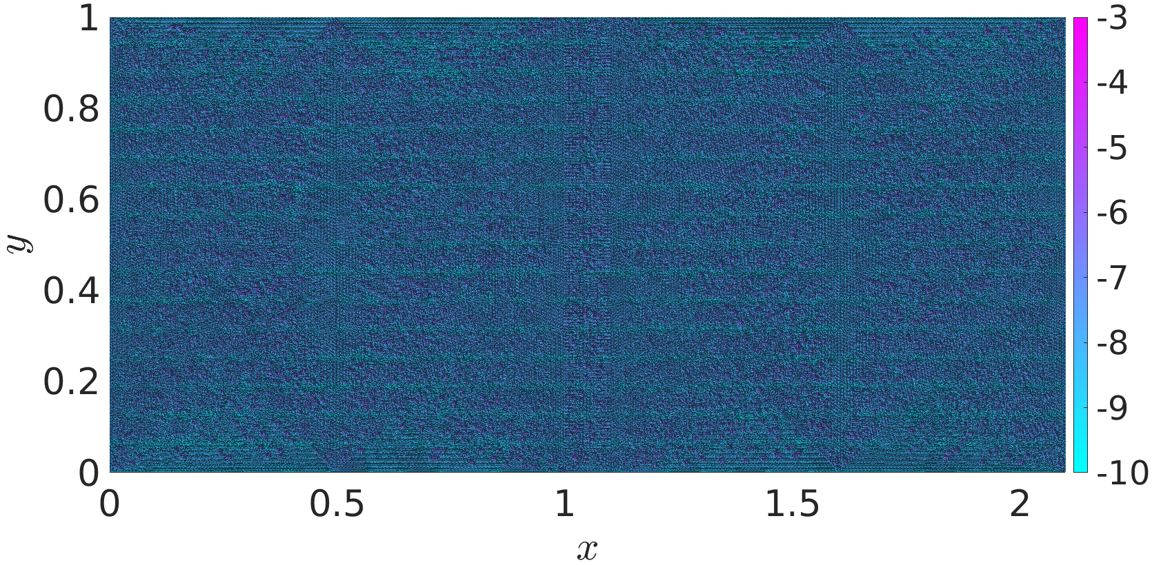
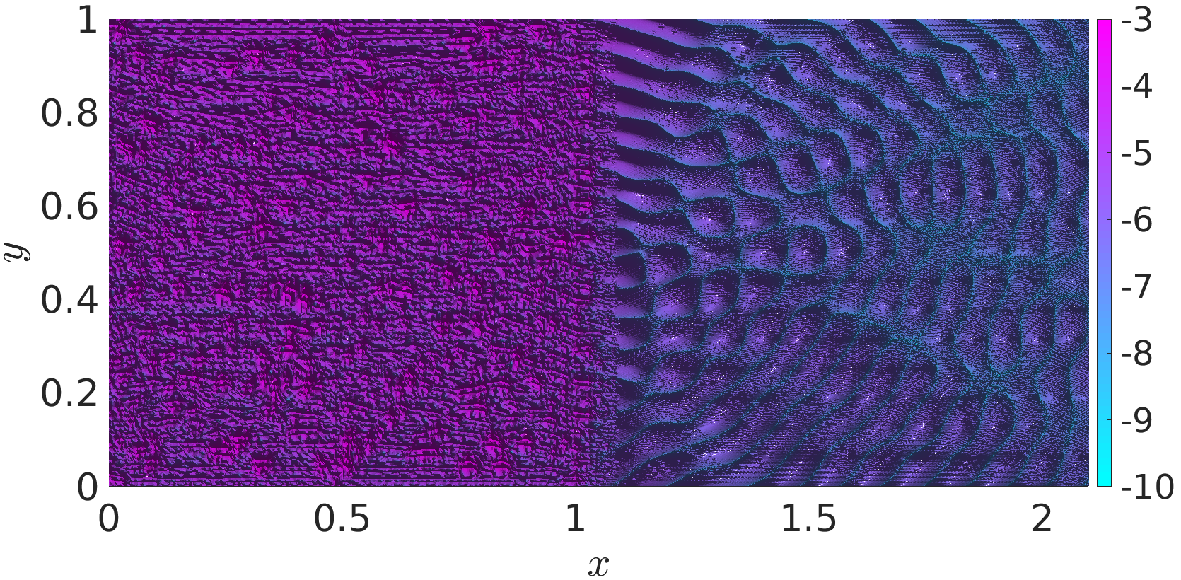
Figure 2.3: Same as Figure 2.2 (including all parameter values) but with $\theta=\pi/2$.

Figures 2.2 and 2.3 plot the FEM error $u-u_{h}$ for all three meshes with $k=50$, $p=4$, $h_{1}=1.78k^{-1}$, $h_{2}=0.38k^{-1}$, $\theta=0$ in Figure 2.2, and $\theta=\pi/2$ in Figure 2.3. The errors are plotted on a logarithmic scale, with the scale kept the same for all the plots.

In both Figures 2.2 and 2.3, for the third mesh the error in the right-hand square (with mesh width $h_{2}$) is between 10 to 100 times larger than the error in the right-hand square for the second (globally $h_{2}$) mesh; i.e., in the right-hand square for the third mesh, the error is dominated by the “slush” term on the right-hand side of (1.8) and not the local best-approximation error. Furthermore, by eye, this “slush” error is low frequency.

The difference between Figures 2.2 and 2.3 is that in the first, the exact solution propagates from left to right, whereas in the second the exact solution propagates upwards. These figures show that the error is affected by the direction of propagation of the solution (or more precisely, its localisation in Fourier space), but does not “inherit” these properties; indeed, in Figure 2.3 the error still propagates from left to right, even though the exact solution propagates upwards.

Experiment 2.

This experiments considers the non-uniform mesh from Experiment 1 with $h_{1}$ and $h_{2}$ now chosen to decrease with $k$ at different rates, with the FEM error computed at a sequence of values of $k$. We do this so that the terms on the right-hand side of (1.8) have different $k$-dependence in the left and right squares.

We take $p=2$, $h_{1}=\sqrt{2}/k$, $h_{2}=1/k^{3/2}$, and $k\in[5,60]$, and Figures 2.4 and 2.5 plot the $H^{1}_{k}$ norm of the error on the left and right, respectively, as well as their high- and low-frequency components (see §2.3 below for how these components are computed).

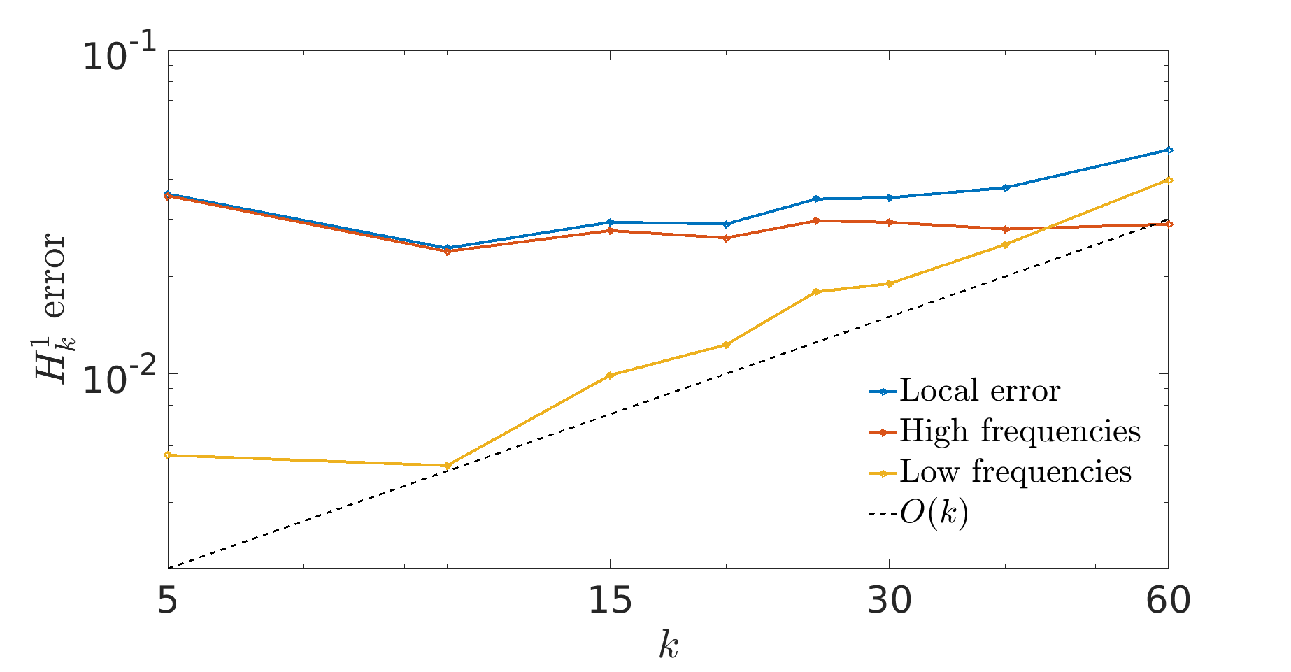
Figure 2.4: For Experiment 2 in §2.1, plots of the $H^{1}_{k}$ error and its low- and high-frequency components in the left square (i.e., the square with the coarser mesh).

Figure 2.5: For Experiment 2 in §2.1, plots of the $H^{1}_{k}$ error and its low- and high-frequency components in the right square (i.e., the square with the finer mesh).

The key point is that, on both the left and right, the FEM solution is locally quasi-optimal, modulo low frequencies, with the low frequencies on the left caused by the pollution effect, and the low frequencies on the right coming from the “slush” term propagating from the left.

In more detail: in Figure 2.4 we see that

(i) the error in the left square grows with $k$,

(ii) the high frequencies of the error are roughly constant in $k$, and

(iii) the growth in the error is caused by the low-frequency components, which are proportional to $k$.

Points (i) and (iii) are expected [19, Corollary 3.2 and Point 1 in the following discussion] which proves that

$$\|u-u_{h}\|_{H^{1}_{k}}\sim k(hk)^{2p}\|u\|_{H^{1}_{k}}\sim k,$$

for the 1-d impedance problem with $hk$ sufficiently small. Point (ii) is expected because the local best approximation error on the left $\sim(hk)^{p}\|u\|_{H^{p+1}}\sim(hk)^{2}\sim 1$; i.e., modulo low frequencies the FEM solution is locally quasi-optimal.

In Figure 2.5 we see that

(iv) The high frequencies decrease like $k^{-1}$.

(v) The low frequencies grow like $k^{1/2}$.

Point (iv) is expected since the local best approximation error on the right $\sim(hk)^{p}\|u\|_{H^{p+1}}\sim(hk)^{2}\sim k^{-1}$.

A heuristic argument for Point (v) is the following. Let $\chi$ be a compactly supported cutoff function supported on the left square, and let $e:=\chi(u-u_{h})$. For sufficiently large $k$, Points (i) to (iii) above show that the low frequencies dominate, and thus we assume that, first, $\mathcal{F}_{k}{e}(\xi)$ is negligible except in the interval $[0,C]$ for some constant $C>1$ and, second, $\mathcal{F}_{k}{e}(\xi)$ is approximately evenly distributed in $[0,C]$. Since the local $H^{1}_{k}$ error on the left $\sim k$,

$$k^{d}\int_{0}^{C}\langle\xi\rangle^{2}{\left\lvert{\mathcal{F}_{k}e(\xi)}\right\rvert}^{2}\,{\rm d}\xi\sim k$$

which implies that ${\left\lvert{\mathcal{F}_{k}e(\xi)}\right\rvert}\sim k^{1/2}k^{-d/2}$ uniformly for $\xi\in[0,C]$. Within the interval $[0,C]$, only the components in $[k-\eta,k+\eta]$ propagate, where $\eta=O(1)$; this is because the Helmholtz operator is (semiclassically) elliptic away from frequency $k$. Therefore, the $H^{1}_{k}$ norm of the error propagated to the right square is approximately

$$k^{d}\int_{k-\eta}^{k+\eta}\langle\xi\rangle^{2}{\left\lvert{\mathcal{F}_{k}e(\xi)}\right\rvert}^{2}\,{\rm d}\xi\sim k^{1/2};$$

i.e., Point (v).

2.2 Experiments with an artificial source term

Geometry of the obstacles considered in the simulations

We consider the following four obstacles.

• No obstacle i.e. $\Omega_{-}=\emptyset$.

• Two flat mirrors, as shown in Figure 6(a).

• One flat mirror, i.e., the obstacle in Figure 6(a) with the left mirror removed.

• Two curved mirrors with an inscribed ellipse, as shown in Figure 6(b).

(a) Flat mirrors

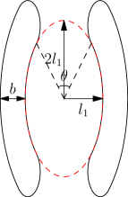
(b) Elliptic mirrors

Figure 2.6: Flat mirror and elliptic mirror geometries.

In all experiments, the computational domain is a disk of radius $1.5$, and the PML region is the annulus $\{1\leq r\leq 1.5\}$. For the one flat mirror, $a=0.4,b=0.2,$ and $L=0.6$. For the two flat mirrors, $a=0.6,b=0.2,$ and $L=0.8$. For the two curved mirrors, $l_{1}=0.265,l_{2}=2l_{1},$ $b=0.17$, and $\theta=\arctan(2\tan(\pi/3))$.

Quasi-resonant wavenumbers for the trapping obstacles

Whereas there is no trapping for the case of no obstacle or one flat mirror, the two flat mirrors and two curved mirrors trap rays. For these latter two geometries, the norm of the solution operator grows faster through an increasing sequence of $k$s (often called “quasi resonances”) than the nontrapping solution operator.

The experiments below for the two flat mirrors and two curved mirrors are conducted at quasi resonances for these obstacles.

For the flat mirrors, the quasi resonances are

$$k_{n}:=n\frac{\pi}{L-b}\,,\quad n=1,2,\ldots.$$

Indeed, for each of those frequencies, one can manufacture a “quasi-mode” of the Laplace operator, in the form $u_{n}(x,y)=\chi(y)\psi(x)\sin(k_{n}x)$ where $\chi$ is a cutoff function supported in $(-a/2,a/2)$, and $\psi$ is a cutoff function with $\psi\equiv 1$ on $[-L/2+b/2,L/2-b/2]$ and supported in $[-L-b/2,L+b/2]$.

For the curved mirrors, the Helmholtz solution operator grows exponentially through the square roots of eigenvalues of the Laplace operator with Dirichlet conditions in the domain $U$ equal to the ellipse inscribed between the mirrors. By separation of variables, these quasi resonances can be expressed as zeros of some special Mathieu functions (see [22, Appendix E]) and computed accordingly (see, e.g.,[29] and associated Matlab toolbox).

The artificial source term.

Let $g:=\Delta u+k^{2}u$, where

$$u(x,y):=\chi(x)\chi(y)\exp({\rm i}kx)\quad\text{ and }\quad\chi(x)=\begin{cases}0&\textup{for }\sqrt{x^{2}+y^{2}}\geq 0.1\\ \exp\left(\frac{5(x^{2}+y^{2})}{x^{2}+y^{2}-0.01}\right)&\textup{otherwise.}\end{cases}$$

Observe that $u$ is supported in $\Omega_{\square}:=[-0.1,0.1]^{2}$.

The FEM error.

Figure 2.7 plots the FEM error (on a logarithmic scale) with $hk=1$ and $p=4$. For the two nontrapping obstacles (i.e., no obstacle and the one flat mirror) $k=100$. For the two trapping obstacles $k$ is taken to be the closest quasi resonance to $100$, namely $k=104.72$ for the two flat mirrors and $k=95.838$ for the two curved mirrors.

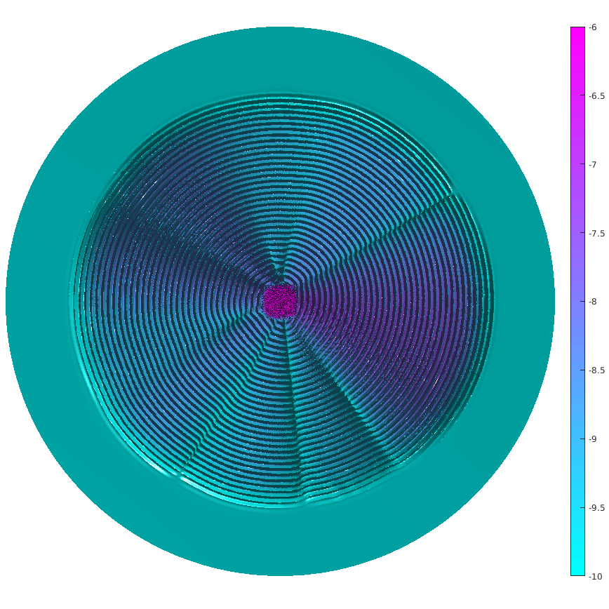
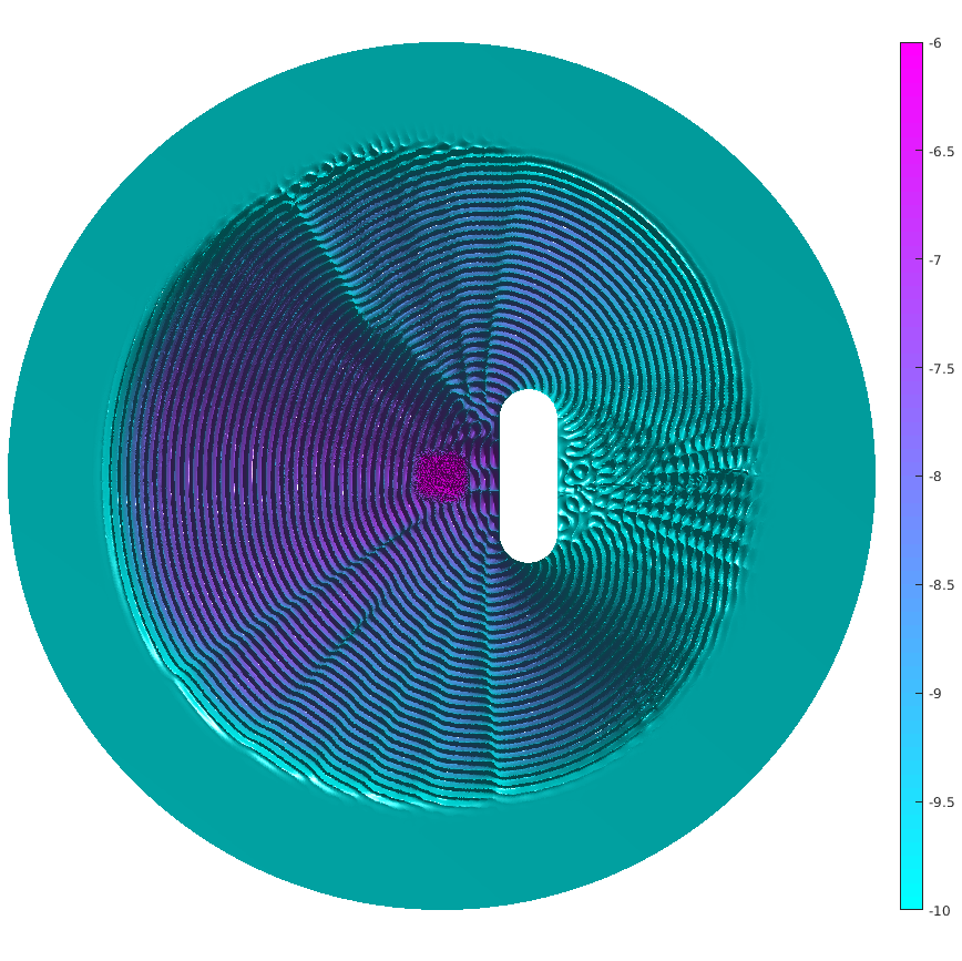
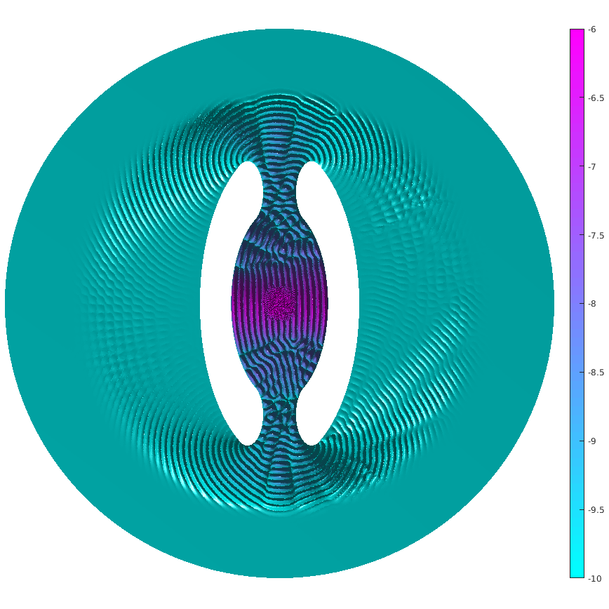
Figure 2.7: For the experiment in §2.2 with $k\approx 100$, $hk=1$ and $p=4$, the plots show $\log({\left\lvert{\Re(u-u_{h})}\right\rvert})/\log(10)$ (the rationale for plotting the real part and not the absolute value is to give a sense of the wave-length). Plots obtained with FFMATLIB.

All four of the figures show a large high-frequency error on the support of $u$ (i.e., on $\Omega_{\square}$) and a small low-frequency error away from the support of $u$. Since the best approximation error is zero away from the support of $u$, this is consistent with the claim that Helmholtz FEM solutions are quasi optimal modulo low frequencies.

The four figures also show that, whereas the high-frequency error in $\Omega_{\square}$ is roughly the same in all four cases, the low-frequency error is affected by the shape of the obstacles. Indeed, for the two trapping obstacles the “slush” is larger inside the trapping regions than elsewhere, and for the three non-empty obstacles the “slush” is smaller in the shadow regions.

To quantify the high- and low-frequency behaviour more precisely, for each obstacle we consider two boxes: $\Omega_{\square}$ and a location away from the source (described for each obstacle in the caption of Table 2.1). In each box we let $v_{h}=\chi(u-u_{h})$, where $\chi$ is a cut-off function compactly supported in each box, and we compute the high- and low-frequency components of $v_{h}$ as described in §2.3 below.

For the “one mirror” obstacle, $v_{h}$ in the two different boxes is plotted in Figure 2.8 for $k=50$. Figure 2.9 plots the Discrete Fourier Transform (DFT) of $v_{h}$ in base $10$ log scale; these plots confirm that the error away from $\Omega_{\square}$ (in the left plot) is dominated by low frequencies, compared to the error in $\Omega_{\square}$ (in the right plot).

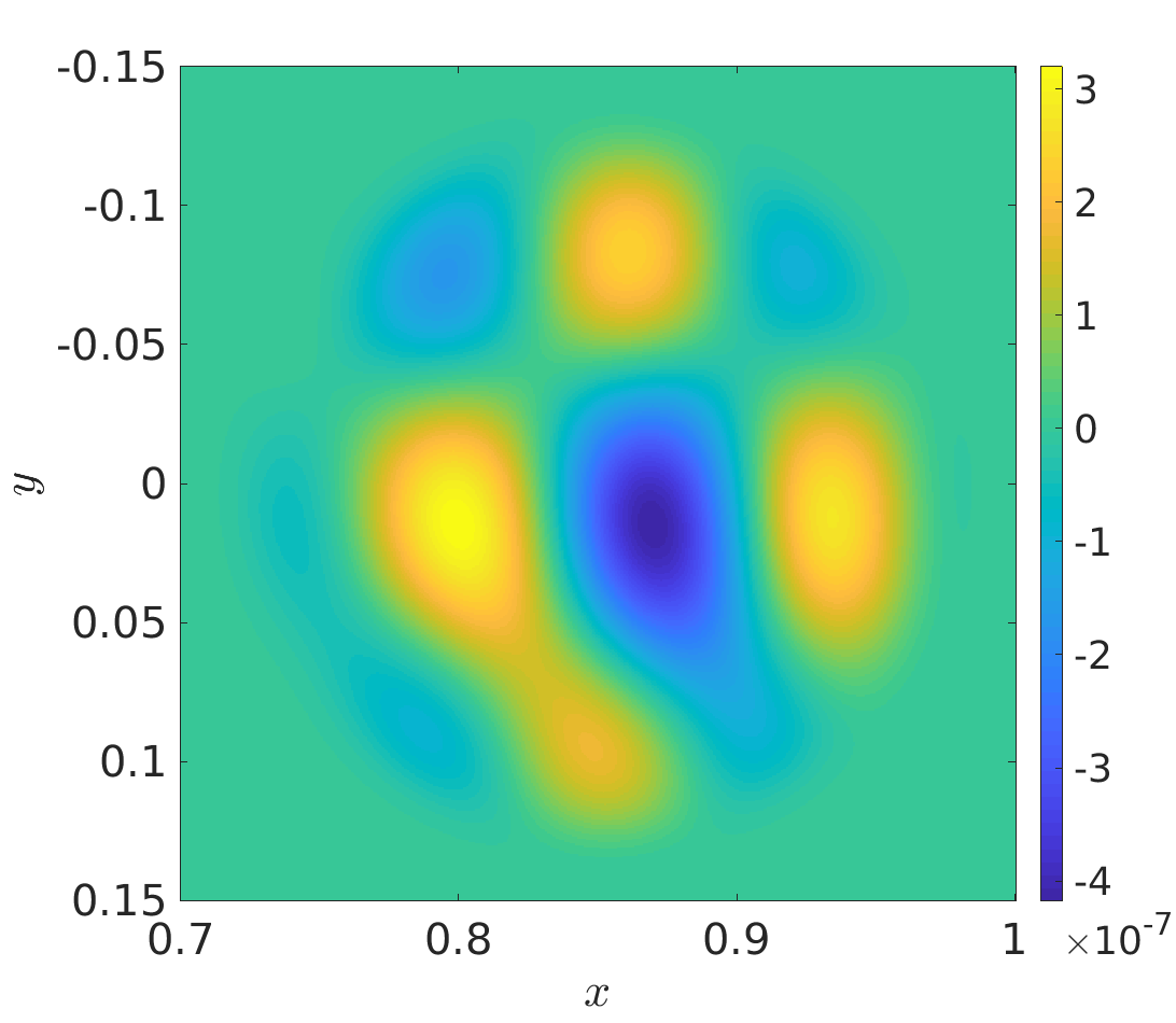
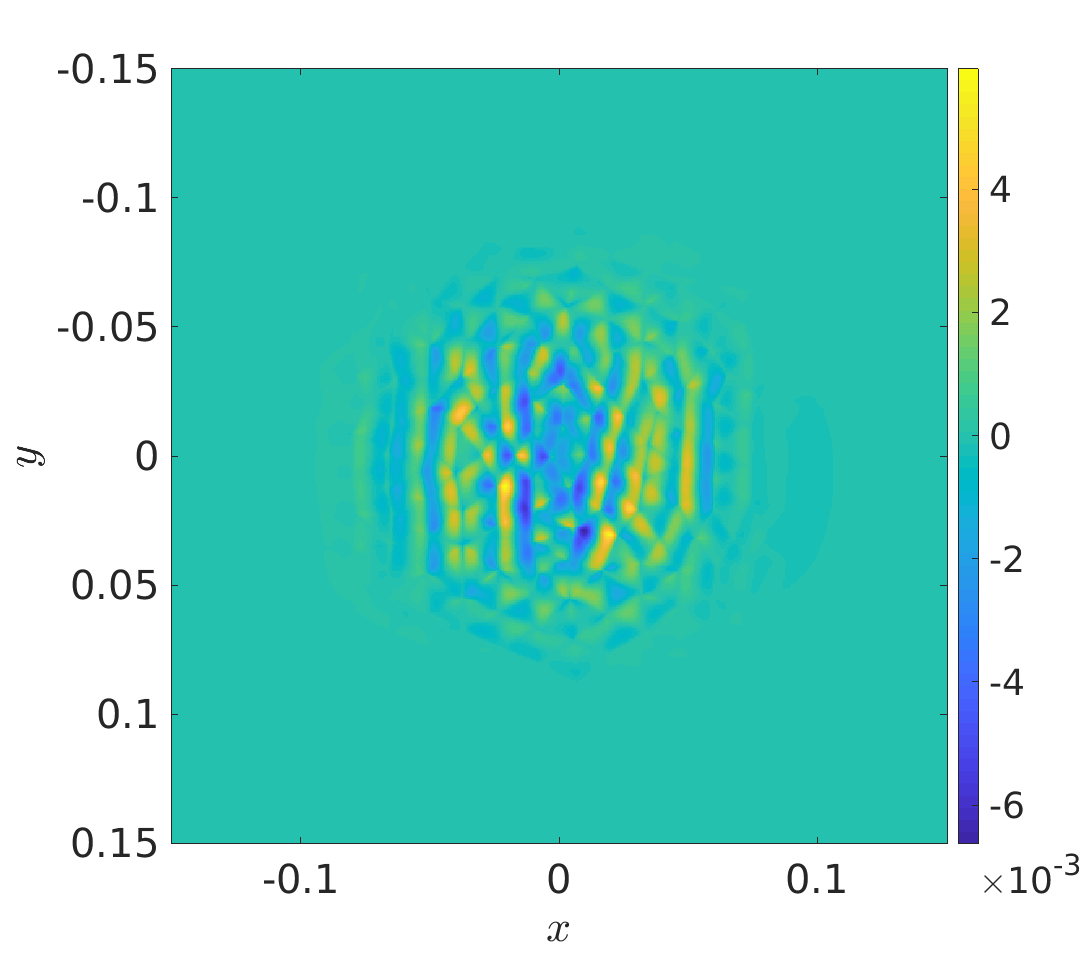
Figure 2.8: The signal $V$ corresponding to the scattering by “one wall” (see Figure 2.7, top right) with $k=50$ and $\Delta=10^{-3}$. Left: $x_{0}=0.7$, $y_{0}=-0.15$ (thus, the box is on the right of the wall, and the error is “pure slush”. Right: $x_{0}=y_{0}=-0.15$ (thus, the box contains $\Omega_{\square}$).

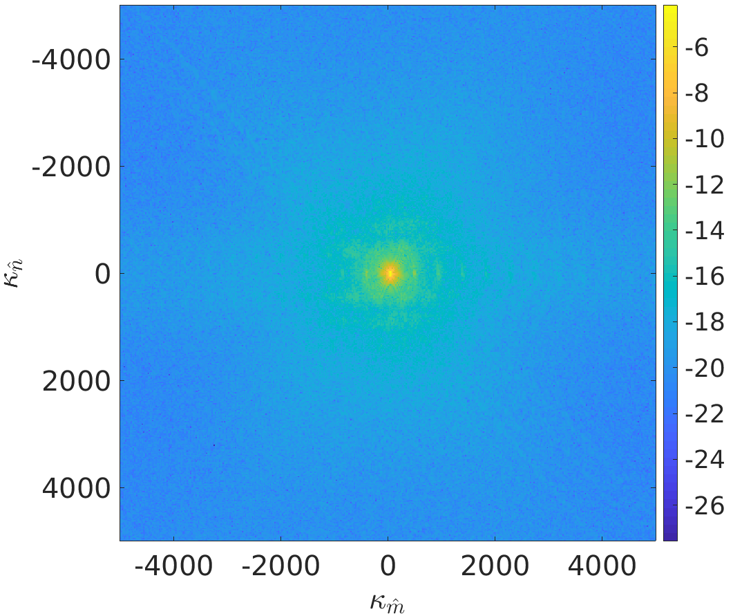
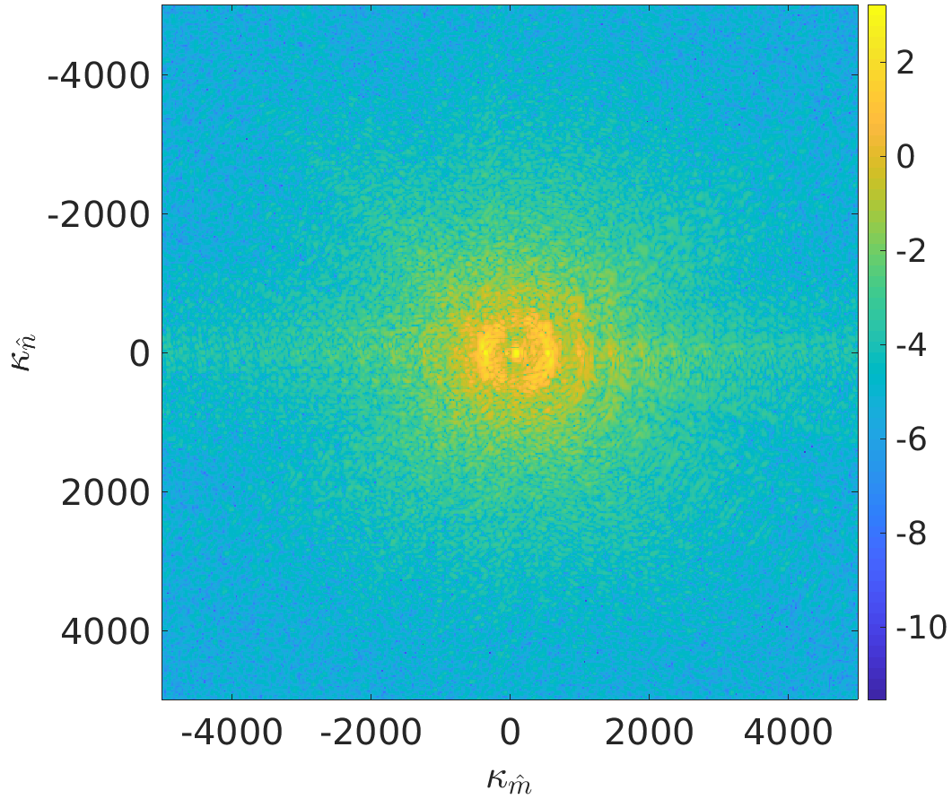
Figure 2.9: Graph of $\log(|\widehat{V}|)$, where in each figure, $\widehat{V}$ is the Discrete Fourier Transform of the corresponding $V$ in Figure 2.8. This confirms that error away from $\Omega_{\square}$ (left) is dominated by low frequencies, compared to the error in $\Omega_{\square}$ (right).

Tables 2.1 and 2.2 plot the quantity $\rho$ defined by (2.1) below, which measures the proportion of the high-frequencies of $v_{h}$. As expected, the values of $\rho$ are much smaller in the “away” region than in $\Omega_{\square}$.

Experiment	$k=50$	$k=75$	$k=100$
a) no obstacle	0.0593	0.0165	0.0091
b) one flat mirror	0.0625	0.0183	0.0103
c) two flat mirrors	0.0471	0.0251	0.0122
d) two curved mirrors	0.0460	0.0236	0.0186

Table 2.1: Values of $\rho$ (cf eq. (2.1)) in experiments a)-d) for a box away from $\Omega_{\square}$. For the experiments a)-b) , the box is defined by $x_{0}=0.7$, $y_{0}=-0.15$. In c) and d), we use $x_{0}=-0.15$ and $y_{0}=0.2$ (thus the boxes are inside the cavities). We take $\Delta=(20k)^{-1}$. In all cases, $N\Delta=0.3$ (i.e., the box sides are 0.3). The polynomial degree of the FEM is set to $p=2$ in these experiments.

Experiment	$k=50$	$k=75$	$k=100$
a) no obstacle	0.9379	0.8421	0.8142
b) one flat mirror	0.9375	0.8700	0.8001
c) two flat mirrors	0.9342	0.8726	0.8043
d) two curved mirrors	0.9532	0.9177	0.5817

Table 2.2: Values of $\rho$ (cf eq. (2.1)) in experiments a)-d) for the box $[-0.15,0.15]^{2}\supset\Omega_{\square}$.

2.3 Computing the high- and low-frequency components

To compute the high- and low-frequency components of a finite-element function $v_{h}$ restricted to a square, we compute the 2-dimensional discrete Fourier transform of the matrix ${V}$ defined by

$${V}_{m,n}=v_{h}(x_{m},y_{n})\,,\quad 0\leq m,n\leq N-1$$

where $x_{m}=x_{0}+m\Delta$, $y_{n}=y_{0}+n\Delta$ and the sampling rate $\Delta^{-1}$ is chosen sufficiently large (in our tests, we use $\Delta=2\pi/(200k)$ and compare with $\Delta=2\pi/(400k)$ to confirm that the results are not very sensitive to this value). This interpolation from a triangular mesh to a Cartesian grid is performed with the help of the FFMATLIB toolbox.

Let ${\widehat{V}}$ be the discrete Fourier Transform of ${V}$, that is

$$\widehat{V}_{\widehat{m},\widehat{n}}=\sum_{m=0}^{N}\sum_{n=0}^{N}V_{m,n}{\rm e}^{-\frac{2{\rm i}\pi}{N}(\widehat{m}m+\widehat{n}n)}\,,$$

so that

$$v_{h}(x_{m},y_{n})=\frac{1}{N^{2}}\sum_{\widehat{m}=1}^{N}\sum_{\widehat{n}=1}^{N}\widehat{W}_{\widehat{m},\widehat{n}}{\rm e}^{{\rm i}\kappa_{\widehat{m}}x_{m}}{\rm e}^{{\rm i}\kappa_{\widehat{n}}y_{n}}\,,\quad 0\leq m,n\leq N-1\,,$$

with

$$\widehat{W}_{\widehat{m},\widehat{n}}=\widehat{V}_{\widehat{m},\widehat{n}}{\rm e}^{-{\rm i}(\kappa_{\widehat{m}}x_{0}+\kappa_{\widehat{n}}y_{0})}\,,\quad\kappa_{\widehat{m}}=\frac{2\pi}{\Delta}\frac{\widehat{m}}{N}\,.$$

That $v_{h}$ is low frequency means that one can represent it accurately as a linear combination of waves of the form ${\rm e}^{{\rm i}\kappa_{1}x}{\rm e}^{{\rm i}\kappa_{2}y}$ with $\kappa_{1},\kappa_{2}\lesssim k$. Here we check this by computing the discrete signal

$$\widetilde{v}_{h}(x_{n},y_{n}):=\frac{1}{N^{2}}\sum_{\widehat{m}=1}^{N}\sum_{\widehat{n}=1}^{N}\widehat{H}_{\widehat{m}}\widehat{H}_{\widehat{n}}\widehat{W}_{\widehat{m},\widehat{n}}{\rm e}^{{\rm i}\kappa_{\widehat{n}}x_{n}}{\rm e}^{{\rm i}\kappa_{\widehat{m}}y_{n}}\,,$$

where $H$ is a “low-pass filter”, i.e.

$$\widehat{H}_{\widehat{m}}=\begin{cases}1&\textup{if }\widehat{\kappa}_{\widehat{m}}\leq\alpha k\textup{ or }\frac{2\pi}{\Delta}-\widehat{\kappa}_{\widehat{m}}\leq\alpha k\,,\\ 0&\textup{otherwise.}\end{cases}$$

Note that, by periodicity, for all $0\leq m,\widehat{m}\leq N-1$, one has

$${\rm e}^{{\rm i}\widehat{\kappa}_{\hat{m}}x_{m}}={\rm e}^{-{\rm i}(\frac{2\pi}{\Delta}-\widehat{\kappa}_{\hat{m}})x_{m}}\,,$$

hence $\widehat{H}$ effectively removes all frequencies outside the interval $[-\alpha k,\alpha k]$. Here, $\alpha$ is a parameter, set to $2$ in our tests.

The relative $l^{2}$ norm of the high-frequency components of $v_{h}$ is

$$\rho:=\frac{{\left\lVert{v_{h}-\widetilde{v}_{h}}\right\rVert}_{l^{2}}}{{\left\lVert{v_{h}}\right\rVert}_{l^{2}}}\,,$$ (2.1)

where ${\left\lVert{\cdot}\right\rVert}_{l^{2}}$ is the discrete $l^{2}$ norm. By Parseval’s theorem for discrete Fourier transforms, this ratio is equal to

$$\rho=\frac{\sum_{\widehat{m},\widehat{n}=1}^{N}(1-\widehat{H}_{\hat{m}}\widehat{H}_{\widehat{n}})^{2}{\left\lvert{\widehat{V}_{\widehat{m},\widehat{n}}}\right\rvert}^{2}}{\sum_{\widehat{m},\widehat{n}=1}^{N}{\left\lvert{\widehat{V}_{\widehat{m},\widehat{n}}}\right\rvert}^{2}}\,.$$

3 Abstract framework

3.1 Function spaces

Given a Hilbert space $\mathcal{Y}$, let $\mathcal{Y}^{*}$ be the Hilbert space of bounded anti-linear functionals $G:\mathcal{Y}\to\mathbb{C}$ (i.e. $G(\lambda y)=\overline{\lambda}G(y)$) equipped with the norm

$${\left\lVert{G}\right\rVert}_{\mathcal{Y}^{*}}:=\sup_{y\in\mathcal{Y}\setminus\{0\}}\frac{|G(y)|}{{\left\lVert{y}\right\rVert}_{\mathcal{Y}}}.$$ (3.1)

Let $\Omega\subset\mathbb{R}^{d}$ be a bounded open set and let $\mathcal{H}:=L^{2}(\Omega)$. As usual, $\mathcal{H}$ is identified with its dual $\mathcal{H}^{*}$. Furthermore, let $k_{0}>0$ and let $(\mathcal{Z}_{k})_{k\geq k_{0}}$ be a family of Hilbert spaces such that for each $k\geq k_{0}$, the inclusion $\mathcal{Z}_{k}\subset\mathcal{H}$ is dense. In all the examples below, ${\cal Z}_{k}$ is either $H^{1}_{k}(\Omega)$ or this space with a Dirichlet boundary condition prescribed on a subset of its boundary. However, ${\cal Z}_{k}$ could also, for example, be a piecewise $H^{1}$ space with a prescribed jump condition between the pieces. To quantify abstractly the “regularity” of elements of $\mathcal{H}$, we introduce a scale of Hilbert spaces $(\mathcal{Z}_{k}^{j})_{0\leq j\leq\ell+2}$ with $\mathcal{Z}_{k}^{0}=\mathcal{H}$, $\mathcal{Z}_{k}^{1}=\mathcal{Z}_{k}$, and with dense inclusions $\mathcal{Z}_{k}^{j}\subset\mathcal{Z}_{k}^{j-1}$ for $j=1,\dots,\ell+2$.

For $j\geq 0$, each anti-linear functional $g$ on $\mathcal{Z}_{k}^{j}$ also defines an anti-linear functional on $g^{\prime}$ on $\mathcal{Z}_{k}^{j^{\prime}}$ for $j^{\prime}\geq j$, via restriction since $\mathcal{Z}_{k}^{j^{\prime}}\subset\mathcal{Z}_{k}^{j}$. This restriction map is moreover continuous and injective, by density of the previous inclusions and hence we identify $g$ and $g^{\prime}$. This identification is compatible with the identification of $\mathcal{H}$ to its dual, and gives the chain of continuous and dense inclusions

$$(\mathcal{Z}_{k}^{\ell+1})^{*}\supset(\mathcal{Z}_{k}^{\ell})^{*}\supset\ldots\supset(\mathcal{Z}_{k}^{1})^{*}\supset\underbrace{\mathcal{Z}_{k}^{0}}_{=\mathcal{H}}\supset\underbrace{\mathcal{Z}_{k}^{1}}_{=\mathcal{Z}_{k}}\supset\ldots\supset\mathcal{Z}_{k}^{\ell}\supset\mathcal{Z}_{k}^{\ell+1}\,.$$ (3.2)

We assume that there exists $C_{\rm emb}>0$ such that

$${\left\lVert{u}\right\rVert}_{\mathcal{Z}_{k}^{j}}\leq C_{\rm emb}{\left\lVert{u}\right\rVert}_{\mathcal{Z}^{j^{\prime}}_{k}}\,\quad\text{ for all }k\geq k_{0}\quad\text{ and }\quad 0\leq j\leq j^{\prime}\leq\ell+2,$$ (3.3)

which also implies that ${\left\lVert{u}\right\rVert}_{(\mathcal{Z}_{k}^{j^{\prime}})^{*}}\leq C_{\rm emb}{\left\lVert{u}\right\rVert}_{(\mathcal{Z}_{k}^{j})^{*}}$ for $0\leq j\leq j^{\prime}\leq\ell+2$.

For technical reasons (to be able to treat transmission problems), we introduce another scale $(\mathcal{W}_{k}^{j})_{0\leq j\leq\ell+1}$ of Hilbert spaces with the property that $\mathcal{Z}_{k}^{j}\subset\mathcal{W}_{k}^{j}\subset\mathcal{H}$ with continuous inclusions (in particular $\mathcal{W}_{k}^{0}=\mathcal{H}$), and

$${\left\lVert{u}\right\rVert}_{\mathcal{W}_{k}^{j}}\leq C_{\rm emb}{\left\lVert{u}\right\rVert}_{\mathcal{Z}^{j}_{k}}\,\quad\text{ for all }k\geq k_{0}\quad\text{ and }\quad 0\leq j\leq\ell+2.$$ (3.4)

Example 3.1

For the Helmholtz transmission problem with the outgoing condition approximated by a perfectly-matched layer,

$${\cal Z}_{k}=H^{1}_{0}(\Omega),\quad{\cal W}^{j}_{k}=L^{2}(\Omega)\cap\big{(}H^{j}(\Omega_{\rm in})\oplus H^{j}(\Omega_{\rm out}\cap\Omega)\big{)},\quad\text{ and }\quad{\cal Z}^{j}_{k}={\cal W}^{j}_{k}\cap H^{1}_{0}(\Omega),$$

where $\Omega_{\rm in}$ is the penetrable obstacle, $\Omega_{\rm out}$ its exterior, and $\Omega$ the (truncated) computational domain containing $\Omega_{\rm in}$; see §7.2 below.

3.2 Local properties

Lemma 3.2

Let $B_{j},j=1,\ldots,N$ be open sets, and let

$$C:=\max\Big{\{}|J|:B_{j_{1}}\cap\ldots\cap B_{j_{J}}\neq\emptyset\text{ with $j_{1},\ldots,j_{J}$ distinct}\Big{\}}.$$

Then

$$C^{-1}\sum_{j=1}^{N}\left\|v\right\|^{2}_{{\cal H}(B_{j})}\leq\left\|v\right\|^{2}_{{\cal H}(\cup_{j=1}^{N}B_{j})}\leq\sum_{j=1}^{N}\left\|v\right\|^{2}_{{\cal H}(B_{j})}$$ (3.5)

for all $v\in{\cal H}(\cup_{j=1}^{N}B_{j})$.

The notation $B_{j}$ is used because we use Lemma 3.2 below with the $B_{j}$ either balls or balls intersected with some larger (fixed) open set.

Proof of Lemma 3.2. The second inequality in (3.5) follows immediately from the fact that the ${\cal H}$ norm is the $L^{2}$ norm. Given $x\in\cup_{j=1}^{N}B_{j}$ let $m(x)$ be the number of distinct $B_{1},\ldots,B_{N}$ that contain $x$. Then

$$\sum_{j=1}^{N}\left\|v\right\|^{2}_{{\cal H}(B_{j})}=\int_{\cup_{j=1}^{N}B_{j}}m(x)|v(x)|^{2}\,{\rm d}x$$

and the first inequality in (3.5) follows since $|m(x)|\leq C$.   

Assumption 3.3

The following holds with ${\cal Y}$ equal to either ${\cal W}$ or ${\cal Z}$. Given open sets $B_{1},\ldots,B_{N}$, with $C$ as in (3.2),

$$C^{-1}\sum_{j=1}^{N}\left\|v\right\|^{2}_{{\cal Y}_{k}^{j}(B_{j})}\leq\left\|v\right\|^{2}_{{\cal Y}_{k}^{j}(\cup_{j=1}^{N}B_{j})}\leq\sum_{j=1}^{N}\left\|v\right\|^{2}_{{\cal Y}_{k}^{j}(B_{j})}$$ (3.6)

for all $v\in{\cal Y}_{k}^{j}(\cup_{j=1}^{N}B_{j})$. Furthermore, if ${\rm supp}\,u\cap{\rm supp}\,v=\emptyset$, then

$$\|u+v\|_{{\cal Y}_{k}^{j}}^{2}=\|u\|_{{\cal Y}_{k}^{j}}^{2}+\|v\|_{{\cal Y}_{k}^{j}}^{2}.$$ (3.7)

With $\partial_{<}$ defined by (1.4), for $U\subset\Omega$ open, let

$$\mathcal{Z}_{k}^{j,<}(U) :=\overline{\big{\{}v\in\mathcal{Z}_{k}^{j}\textup{ s.t. }{\rm supp}\,v\subset\overline{U},\,\partial_{<}({\rm supp}\,v,\overline{U})>0\big{\}}}$$

$$\,\,=\overline{\big{\{}v\in\mathcal{Z}_{k}^{j}\textup{ s.t. }{\rm supp}\,v\subset U\cup(\partial U\cap\partial\Omega)\big{\}}}$$ (3.8)

(where the closures are taken with respect to the ${\cal Z}^{j}_{k}$ norm). Observe that the convention that $\partial_{<}(A,B)=+\infty$ when $B=\Omega$ implies that $\mathcal{Z}_{k}^{j,<}(\Omega)=\mathcal{Z}_{k}^{j}$.

For any $U\subset\Omega$, let

$$\|u\|_{{\cal Z}_{k}^{j}(U)}:=\inf\Big{\{}\|v\|_{\mathcal{Z}_{k}^{j}}\,:\,v|_{U}=u|_{U},\,v\in\mathcal{Z}_{k}^{j}\Big{\}};$$ (3.9)

observe that this definition implies that $\|u\|_{{\cal Z}_{k}^{j}(U)}\leq\|u\|_{{\cal Z}_{k}^{j}(V)}$ for $U\subset V$.

For an open set $U\subset\Omega$ and $j\geq 0$, observe that (3.1) implies that

$${\left\lVert{u}\right\rVert}_{(\mathcal{Z}_{k}^{j,<}(U))^{*}}=\sup_{v\in\mathcal{Z}_{k}^{j,<}(U)\setminus\{0\}}\frac{|u(v)|}{{\left\lVert{v}\right\rVert}_{\mathcal{Z}_{k}^{j}}}\,.$$ (3.10)

Since $\mathcal{Z}_{k}^{j,<}(\Omega)=\mathcal{Z}_{k}^{j}$, ${\left\lVert{\cdot}\right\rVert}_{(\mathcal{Z}_{k}^{j,<}(\Omega))^{*}}={\left\lVert{\cdot}\right\rVert}_{(\mathcal{Z}^{j}_{k})^{*}}$.

We define ${\cal W}^{j,<}_{k}(U)$ and ${\left\lVert{\cdot}\right\rVert}_{(\mathcal{W}_{k}^{j,<}(U))^{*}}$ analogously to (3.8) and (3.10).

3.3 Sesquilinear forms

We consider a family $(a_{k})_{k\geq k_{0}}$ of sesquilinear forms $a_{k}:\mathcal{Z}_{k}\times\mathcal{Z}_{k}\to\mathbb{C}$ (i.e. $a_{k}(\lambda u,\mu v)=\lambda\overline{\mu}a_{k}(u,v)$), satisfying the following assumptions.

Assumption 3.4 (Continuity and local coercivity)

There exist positive constants ${C_{\rm cont}}$, ${c_{\rm coer}}$, and ${C_{\rm coer}}$ such that

$$|a_{k}(u,v)|\leq{C_{\rm cont}}\left\|u\right\|_{\mathcal{Z}_{k}}\left\|v\right\|_{\mathcal{Z}_{k}}\quad\text{ for all }u,v\in\mathcal{Z}_{k}\text{ and }k\geq k_{0}$$ (3.11)

and if $x_{0}\in\Omega$ and $r\leq{c_{\rm coer}}k^{-1}$ then

$$\Re\big{\{}a_{k}(v,v)\big{\}}\geq{C_{\rm coer}}\left\|v\right\|^{2}_{{\cal Z}_{k}}\quad\text{ for all }v\in{\cal Z}^{<}_{k}(B(x_{0},r)\cap\Omega)\text{ and }k\geq k_{0}.$$ (3.12)

Assumption 3.5 (Elliptic regularity up to $\partial\Omega$ for the adjoint problem on ${\cal O}(k^{-1})$ balls)

Given $x_{0}\in\Omega$, $r>0$, and $d>0$, let

$$U_{0}:=B(x_{0},r)\cap\Omega\quad\text{ and }\quad U_{1}:=B(x_{0},r+d)\cap\Omega$$ (3.13)

(so that $\partial_{<}(U_{0},U_{1})=d$).

Given $c>0$, and $\ell\in\mathbb{Z}^{+}$, there exists $C_{\rm ell}>0$ such that if $r+d\leq{c_{\rm coer}}k^{-1}$ and $r,d\geq ck^{-1}$, then, for all $u\in\mathcal{Z}_{k}^{<}({U}_{1})$,

$$\left\|u\right\|_{\mathcal{Z}_{k}^{j+2}(U_{0})}\leq C_{\rm ell}\Big{(}\left\|u\right\|_{\mathcal{H}}+\sup_{\begin{subarray}{c}v\in\mathcal{Z}_{k}^{<}({U}_{1})),\,\|v\|_{(\mathcal{W}_{k}^{j})^{*}}=1\end{subarray}}|a_{k}(v,u)|\Big{)},\quad j=0,\dots,\ell.$$ (3.14)

The following assumption involves “localizing” operators that commute with $a_{k}$ in a weak sense. In all the specific examples in §7, these operators are cut-off functions, but for transmission problems these functions must be defined piecewise and satisfy certain properties across the interface; see Lemma 7.7.

Assumption 3.6 (Compatible localisers)

Given $x_{0}\in\Omega$, $r>0$, and $d>0$, let $U_{0}$ and $U_{1}$ be as in (3.13). There exist constants $C_{\dagger}>0$ and $C_{\rm com}>0$ and a family $\{\psi(U_{0},U_{1})\}_{U_{0}\subset U_{1}}$ of localisers indexed by $U_{0}\subset U_{1}\subset\Omega$, and hence indexed by $x_{0},r,d$, where each $\psi=\psi(U_{0},U_{1}):\mathcal{H}\to\mathcal{H}$ is a self-adjoint operator with the following properties

• With $U_{0}^{\prime}:=B(x_{0},r+d/4)\cap\Omega$ and $U_{1}^{\prime}:=B(x_{0},r+3d/4)\cap\Omega$, for all $u\in\mathcal{H}$,

  $$u\equiv\psi u\textup{ on }U^{\prime}_{0}\,,\quad\psi u\equiv 0\textup{ on }(U^{\prime}_{1})^{c}\,.$$

• $\psi$ maps $\mathcal{Z}_{k}^{j}$ to itself continuously, with

  $${\left\lVert{\psi u}\right\rVert}_{\mathcal{Z}_{k}^{j}}\leq C_{\dagger}\sum_{m=0}^{j}(kd)^{-(j-m)}{\left\lVert{u}\right\rVert}_{\mathcal{Z}_{k}^{m}(U_{1})}\quad\text{ for all }j\in\{0,1,\ldots,\ell+2\},$$ (3.15)

• for all $j=1,\ldots,\ell+1$, and $u,v\in\mathcal{Z}_{k}$,

$${\left\lvert{a_{k}(\psi u,v)-a_{k}(u,\psi v)}\right\rvert}$$

$$\leq\frac{C_{\rm com}}{kd}\left(\sum_{m=0}^{j-1}(kd)^{-m}\right)\min\Big{(}{\left\lVert{u}\right\rVert}_{\mathcal{Z}_{k}^{j}(U_{1}\setminus\overline{U_{0}})}{\left\lVert{v}\right\rVert}_{(\mathcal{W}_{k}^{(j-1),<}(U_{1}\setminus\overline{U_{0}}))^{*}},{\left\lVert{u}\right\rVert}_{(\mathcal{W}_{k}^{(j-1),<}(U_{1}\setminus\overline{U_{0}}))^{*}}{\left\lVert{v}\right\rVert}_{\mathcal{Z}_{k}^{j}(U_{1}\setminus\overline{U_{0}})}\Big{)}.$$ (3.16)

Corollary 3.7 (Mapping properties of the adjoint resolvent operator on ${\cal O}(k^{-1})$ balls)

Let $U_{0}$ and $U_{1}$ be given by (3.13). Suppose that $r+d\leq{c_{\rm coer}}k^{-1}$. Let $\mathcal{R}^{*}:({\cal Z}^{<}_{k}({U}_{1}))^{*}\to\mathcal{Z}_{k}^{<}({U}_{1})$ be the operator defined by the variational problem

$$a_{k}(v,{\cal R}^{*}g)=\overline{\langle g,v\rangle}\quad\text{ for all }v\in\mathcal{Z}_{k}^{<}({U}_{1})\,.$$

Then there exists ${C_{\rm res}}>0$ such that

$${\left\lVert{{\cal R}^{*}g}\right\rVert}_{\mathcal{Z}_{k}^{j+2}(U_{0})}\leq{C_{\rm res}}{\left\lVert{g}\right\rVert}_{{\cal W}^{j}_{k}}\quad\text{ for all }g\in\mathcal{W}_{k}^{j,<}({U}_{1})\,,\,\,j=0\,,\ldots\,,\ell\,.$$

Proof. Since $r+d\leq{c_{\rm coer}}k^{-1}$, $\mathcal{R}^{*}$ is well-defined by Assumption 3.4 and the Lax–Milgram lemma, and

$${\left\lVert{{\cal R}^{*}g}\right\rVert}_{\mathcal{Z}_{k}}\leq\frac{1}{{C_{\rm coer}}}{\left\lVert{g}\right\rVert}_{(\mathcal{Z}_{k}^{<}(U_{1}))^{*}}\,.$$ (3.17)

Let $g\in\mathcal{W}_{k}^{j,<}(U_{1})$. By (3.14), the definition of $\mathcal{R}^{*}$, and the triangle inequality,

$${\left\lVert{\mathcal{R}^{*}g}\right\rVert}_{\mathcal{Z}^{j+2}_{k}(U_{0})} \leq C_{\rm ell}\Big{(}{\left\lVert{\mathcal{R}^{*}g}\right\rVert}_{\mathcal{H}}+\sup_{v\in\mathcal{Z}_{k}^{<}({U}_{1}),\,{\left\lVert{v}\right\rVert}_{(\mathcal{W}^{j}_{k})^{*}}=1}{\left\lvert{\langle g,v\rangle}\right\rvert}\Big{)}\leq C_{\rm ell}\big{(}{\left\lVert{\mathcal{R}^{*}g}\right\rVert}_{\mathcal{H}}+{\left\lVert{g}\right\rVert}_{\mathcal{W}_{k}^{j}}\big{)},$$

and the result follows from (3.17).   

3.4 Triangulation and finite-dimensional subspaces

Let $\mathcal{T}$ be a regular triangulation (in the sense of, e.g., [6, Page 61]) of $\Omega$. For each element $K\in\mathcal{T}$, let $h_{K}:=\textup{diam}(K)$. For simplicity, we assume that

$$h_{K}k\leq C_{\rm ppw}$$ (3.18)

for some $C_{\rm ppw}>0$ (where “ppw” standard for “points per wavelength”); as discussed after Theorem 1.1 for standard finite-element spaces with $p$ fixed, $h_{K}k$ must be chosen as a decreasing function of $k$ to maintain accuracy and thus this assumption is not restrictive.

Assumption 3.8 (Broken norms)

For each $u\in\mathcal{Z}_{k}$ and each element $K$ of $\mathcal{T}$, the restriction of $u$ to $K$ belongs to $H^{1}_{k}(K)$, and

$${\left\lVert{u}\right\rVert}_{\mathcal{Z}_{k}(K)}={\left\lVert{u}\right\rVert}_{H^{1}_{k}(K)}\quad\text{ for all }K\in\mathcal{T}\,.$$ (3.19)

For each $K\in\mathcal{T}$, we assume that $C^{\infty}_{0}(K)\subset\mathcal{Z}_{k}^{j}$ and that

$${\left\lVert{u}\right\rVert}_{\mathcal{Z}_{k}^{j}}={\left\lVert{u}\right\rVert}_{H^{j}_{k}(K)}\quad\text{ for all }u\in C^{\infty}_{0}(K)$$ (3.20)

(where the first norm is defined by (3.9)). Furthermore, there exists a constant $C_{\rm loc}$ such that

$${\left\lvert{a_{k}(u,v)}\right\rvert}\leq C_{\rm loc}\sum_{K\in\mathcal{T}}{\left\lVert{u}\right\rVert}_{H^{1}_{k}(K)}{\left\lVert{v}\right\rVert}_{H^{1}_{k}(K)}\quad\text{ for all }u,v\in\mathcal{Z}_{k}\,.$$ (3.21)

We fix a finite-dimensional space $V_{h}\subset\mathcal{Z}_{k}$ consisting of functions whose restrictions to each $K\in\mathcal{T}$ is in $C^{\infty}(\overline{K})$. For any open subset $U\subset\Omega$, let

$$V_{h}^{<}(U):=\mathcal{Z}_{k}^{<}(U)\cap V_{h}\,.$$

We introduce the following standard assumptions on $V_{h}$:

Assumption 3.9 (Approximation property)

There exist constants $\kappa>0$, $p\in\mathbb{Z}^{+}$ and $C_{\rm approx}>0$ such that the following holds. For each $j\in\{1,\ldots,p+1\}$, given $u\in\mathcal{Z}_{k}^{j}$, there exists $u_{h}\in V_{h}$ such that

$$\sum_{K\in\mathcal{T}}(h_{K}k)^{2(m-j)}{\left\lVert{u-u_{h}}\right\rVert}^{2}_{H^{m}_{k}(K)}\leq C_{\rm approx}{\left\lVert{u}\right\rVert}_{\mathcal{Z}_{k}^{j}}^{2}\quad\text{ for all }u_{h}\in V_{h}\,,\,\,0\leq m\leq j\leq p+1.$$ (3.22)

Furthermore, if $U_{0}\subset U_{1}$ are such that

$$\partial_{<}(U_{0},U_{1})>\kappa\max_{K\cap U_{1}\neq\emptyset}h_{K}$$

and $\textup{supp}\,u\subset U_{0}$, then $u_{h}$ can be chosen in $V_{h}^{<}(U_{1})$.

Assumption 3.10 (Super-approximation property)

For each $C_{\dagger}>0$, there exists constant ${C_{\rm super}}>0$ such that, with $p$ and $\kappa$ as in Assumption 3.9, the following property holds for sets $U_{0}\subset U_{1}\subset\Omega$ given by (3.13) and satisfying

$$d=\partial_{<}(U_{0},U_{1})>4\kappa\max_{K\cap U_{1}\neq\emptyset}h_{K}$$ (3.23)

Let $\chi=\psi(U_{0},U_{1})$ be the localiser associated to $U_{0}$ and $U_{1}$ (given by Assumption 3.6). Then for each $u_{h}\in V_{h}$, there exists $v_{h}\in V_{h}^{<}(U_{1})$ such that, for all $K\in\mathcal{T}$,

$${\left\lVert{\chi^{2}u_{h}-v_{h}}\right\rVert}_{H^{1}_{k}(K)}\leq{C_{\rm super}}\frac{h_{K}}{d}\left[\left(1+\frac{1}{kd}\right){\left\lVert{u_{h}}\right\rVert}_{L^{2}(K)}+{\left\lVert{\chi u_{h}}\right\rVert}_{H^{1}_{k}(K)}\right].$$ (3.24)

The constant $\kappa$ in Assumptions 3.9 and 3.10 is related to the “stencil” of the chosen finite element, i.e., how large the support the finite element basis functions is. For Lagrange finite-elements $\kappa=1$; see §7.4 below.

For any open subset $U\subset\mathbb{R}^{d}$ and any $s\in\mathbb{R}$, we recall that $H^{s}(U)$ is defined as the set of restrictions to $U$ of elements of $H^{s}(\mathbb{R}^{d})$, with a Hilbert structured inherited via

$${\left\lVert{v}\right\rVert}_{H^{s}_{k}(U)}:=\inf_{V\in H^{s}_{k}(\mathbb{R}^{d})\,:\,V|_{U}=v}{\left\lVert{V}\right\rVert}_{H^{s}_{k}(\mathbb{R}^{d})}\,.$$ (3.25)

When $U$ is a Lipschitz domain,

$${\left\lVert{u}\right\rVert}_{H^{-s}_{k}(U)}\sim\sup_{\begin{subarray}{c}{\left\lVert{v}\right\rVert}_{H^{s}_{k}(\mathbb{R}^{d})}=1,\\ {\rm supp}v\subset U\end{subarray}}|(u,v)_{L^{2}}|,$$ (3.26)

where $\sim$ denotes norm equivalence; i.e., $H^{-s}_{k}(U)$ is dual to $\widetilde{H}^{s}_{k}(U)$ defined as the closure of $C^{\infty}_{\rm comp}(U)$ in $H^{s}(\mathbb{R}^{d})$; see [23, Page 77 and Theorem 3.30(i), Page 92].

Assumption 3.11 (Inverse inequalities)

Given $p\in\mathbb{Z}^{+}$ as in Assumption 3.9, there exists ${C_{\rm inv}}>0$ such that, for all $K\in\mathcal{T}$ and $u_{h}\in V_{h}$,

$${\left\lVert{u_{h}}\right\rVert}_{H^{1}_{k}(K)}\leq\frac{{C_{\rm inv}}}{h_{K}k}{\left\lVert{u_{h}}\right\rVert}_{L^{2}(K)}$$ (3.27)

and, for $0\leq s\leq p$,

$${\left\lVert{u_{h}}\right\rVert}_{L^{2}(K)}\leq\frac{{C_{\rm inv}}}{(h_{K}k)^{s}}{\left\lVert{u_{h}}\right\rVert}_{H_{k}^{-s}(K)}.$$ (3.28)

4 Statement of the main results

Theorem 4.1 (General version of Theorem 1.1)

Given positive constants ${C_{\rm cont}}$, ${C_{\rm coer}}$, ${c_{\rm coer}}$, $\kappa$, $p$, $C^{\prime}_{\rm inv}$, $C_{\rm pw}$, $C^{\prime}_{\rm super}$, $C_{\rm com}>0$, and some $C_{0}>0$, there exists a constant $C_{\star}>0$ such that the following holds. Let $(a_{k})_{k\geq k_{0}}$ and $V_{h}\subset\mathcal{Z}_{k}$ satisfy Assumptions 3.4, 3.6, 3.9, 3.10, 3.11, and 3.21, with the constants above. Let $\Omega_{0}\subset\Omega_{1}\subset\Omega$ be arbitrary subsets such that

$$d:=\partial_{<}(\Omega_{0},\Omega_{1})\geq\frac{C_{0}}{k}\quad\text{ and }\quad\max_{K\cap\Omega_{1}\neq\emptyset}h_{K}\leq\frac{C_{1}}{k}$$ (4.1)

where

$$C_{1}:=\frac{1}{4\max\big{\{}1,8\kappa\big{\}}}\min\bigg{\{}\frac{C_{0}}{2},\frac{8{c_{\rm coer}}}{3}\bigg{\}}.$$

If $k\geq k_{0}$ and $u\in\mathcal{Z}_{k}$ and $u_{h}\in V_{h}$ are such that

$$a_{k}(u-u_{h},v_{h})=0\quad\text{ for all }v_{h}\in V_{h}^{<}(\Omega_{1}),$$ (4.2)

then

$${\left\lVert{u-u_{h}}\right\rVert}_{\mathcal{Z}_{k}(\Omega_{0})}\leq C_{*}\Big{(}\min_{w_{h}\in V_{h}}{\left\lVert{u-w_{h}}\right\rVert}_{\mathcal{Z}_{k}(\Omega_{1})}+{\left\lVert{u-u_{h}}\right\rVert}_{\mathcal{H}(\Omega_{1})}\Big{)}.$$ (4.3)

If the triangulation $\mathcal{T}$ is furthermore locally quasi-uniform and Assumption 3.5 (local elliptic regularity) holds, then the result can be improved by weakening the $\mathcal{H}$ norm of the error on the right-hand side.

Theorem 4.2 (General version of Theorem 1.2)

Given positive constants ${C_{\rm cont}}$, ${C_{\rm coer}}$, ${c_{\rm coer}}$, $C_{\rm ell}$, $\kappa$, $p$, $C^{\prime}_{\rm inv}$, $C_{\rm pw}$, $C^{\prime}_{\rm super}$, $C_{\rm com}>0$, and some $C_{0}>0$, there exists a constant $C_{\star}>0$ such that the following holds. Let $(a_{k})_{k\geq k_{0}}$ and $V_{h}\subset\mathcal{Z}_{k}$ satisfy Assumptions 3.4, 3.5, 3.6, 3.9, 3.10, 3.11, and 3.21, with the constants above. Let $\Omega_{0}\subset\Omega_{1}\subset\Omega$ be arbitrary subsets such that

$$d:=\partial_{<}(\Omega_{0},\Omega_{1})\geq\frac{C_{0}}{k}\quad\text{ and }\quad\max_{K\cap\Omega_{1}\neq\emptyset}h_{K}\leq\frac{C_{1}}{k}$$

where

$$C_{1}:=\frac{1}{48(\ell+2)\max\big{\{}1,8\kappa\big{\}}}\min\bigg{\{}\frac{C_{0}}{2},2{c_{\rm coer}}\bigg{\}}.$$

Assume further that $\mathcal{T}$ is quasi-uniform on scale $k^{-1}$, in the sense that, for every ball $B$ of radius at most $3{c_{\rm coer}}/(2k)$, the bound (1.7) holds. If $k\geq k_{0}$ and $u\in\mathcal{Z}_{k}$ and $u_{h}\in V_{h}$ are such that (4.2) holds, then

$${\left\lVert{u-u_{h}}\right\rVert}_{\mathcal{Z}_{k}(\Omega_{0})}\leq C_{*}\bigg{(}\min_{w_{h}\in V_{h}}{\left\lVert{u-w_{h}}\right\rVert}_{\mathcal{Z}_{k}(\Omega_{1})}+{\left\lVert{u-u_{h}}\right\rVert}_{(\mathcal{W}_{k}^{s+1,<}(\Omega_{1}))^{*}}\bigg{)}$$ (4.4)

where $s:=\min\{\ell,p-1\}$.

Remark 4.3 (Galerkin orthogonality)

Given $G\in(\mathcal{Z}_{k})^{*}$, if $u\in\mathcal{Z}_{k}$ satisfies

$$a_{k}(u,v)=G(v)\quad\text{ for all }v\in\mathcal{Z}_{k}$$

and if $u_{h}$ is a solution to the Galerkin equations

$$\text{ find }u_{h}\in V_{h}\,\text{ such that }\,a(u_{h},v_{h})=G(v_{h})\quad\text{ for all }v_{h}\in V_{h},$$ (4.5)

then

$$a(u-u_{h},v_{h})=0\quad\text{ for all }v_{h}\in V_{h},$$

and thus $u-u_{h}$ satisfies (4.2) since $V_{h}^{<}(U_{1})\subset V_{h}$.

Remark 4.4 (The dependence of the constant $C^{*}$ on the subspace $V_{h}$)

We have stated Theorem 4.1 for a fixed finite-dimensional subspace $V_{h}\subset\mathcal{Z}_{k}$. The key point is that the constant $C^{*}$ depends quantitatively on $V_{h}$ only through the constants in the assumptions of Section 3. In general, one is interested in applying Theorem 4.1 to a family of subspaces indexed by some parameter (e.g., the mesh parameter $h$ of a sequence of quasi-uniform triangulations $(\mathcal{T}_{h})_{h>0}$ of $\Omega$). The idea is that the bound (4.3) will hold with a common constant $C^{*}$ for all subspaces of the sequence, provided that the assumptions of Section 3 hold uniformly for all of those subspaces. We show in §7.4 that these assumptions do hold uniformly for standard choices of discretisation.

In the rest of the paper we use the letter $C$ in estimates of the form $a\leq Cb$ to represent a generic positive constant, whose numerical value is allowed to change from one place to another, but which can be expressed as a function of the constants in the assumptions of Section 3.

5 Caccioppoli estimates

The central idea in the proofs of Theorems 4.1-4.2 is to apply a discrete version of the classical Caccioppoli inequality to a solution of the Helmholtz equation at the discrete level.

In this section we always assume (without stating explicitly) that $(a_{k})_{k\geq k_{0}}$ and $V_{h}$ satisfy the assumptions of Section 3.

Lemma 5.1 (Caccioppoli estimate in the $L^{2}$ norm on ${\cal O}(k^{-1})$ balls)

There exists a constant $C_{\rm ca}>0$ (whose value depends only on the constants appearing in the assumptions of Section 3 apart from $C_{\rm ell}$) such that, given $r,d>0$, if $U_{0}$ and $U_{1}$ are as in (3.13) (so that $d=\partial_{<}(U_{0},U_{1})$),

$$d\geq\max\left\{1,8\kappa\right\}\max_{K\cap U_{1}\neq\emptyset}h_{K},$$ (5.1)

and

$$r+\frac{d}{2}\leq\frac{{c_{\rm coer}}}{k},$$ (5.2)

then the following holds. If $z_{h}\in V_{h}$ satisfies

$$a_{k}(z_{h},v_{h})=0\quad\textup{for all }v_{h}\in V_{h}^{<}(U_{1})$$ (5.3)

and $k\geq k_{0}$, then

$${\left\lVert{z_{h}}\right\rVert}_{\mathcal{Z}_{k}(U_{0})}\leq\frac{C_{\rm ca}}{kd}{\left\lVert{z_{h}}\right\rVert}_{\mathcal{H}(U_{1})}.$$ (5.4)

Note that the combination of (5.1) and (5.2) imply that $\max_{K\in U_{1}}h_{K}$ is bounded by a constant multiple of $k^{-1}$.

Proof of Lemma 5.1. Let

$$U_{1/2}:=B(0,r+d/2)\cap\Omega$$

so that

$$\partial_{<}(U_{0},U_{1/2})=d/2,\quad\partial_{<}(U_{1/2},U_{1})=d/2.$$ (5.5)

Let $\chi=\psi(U_{0},U_{1/2})$ be the localiser defined in Assumption 3.6. If we can show that

$${\left\lVert{\chi z_{h}}\right\rVert}^{2}_{\mathcal{Z}_{k}}\leq\frac{C}{(kd)^{2}}{\left\lVert{z_{h}}\right\rVert}^{2}_{\mathcal{H}(U_{1})},$$ (5.6)

then the result follows since, by (3.9),

$${\left\lVert{z_{h}}\right\rVert}^{2}_{\mathcal{Z}_{k}(U_{0})}={\left\lVert{\chi z_{h}}\right\rVert}^{2}_{\mathcal{Z}_{k}(U_{0})}\leq{\left\lVert{\chi z_{h}}\right\rVert}_{\mathcal{Z}_{k}}^{2}.$$

The inequality (5.2) and the assumption (3.12) imply that $a_{k}$ is coercive on ${\cal Z}_{k}^{<}(U_{1/2})$. Since $\chi z_{h}\in{\cal Z}_{k}^{<}(U_{1/2})$,

$${\left\lVert{\chi z_{h}}\right\rVert}_{\mathcal{Z}_{k}}^{2}\leq({C_{\rm coer}})^{-1}\big{|}{a}_{k}(\chi z_{h},\chi z_{h})\big{|}.$$

Then, by (3.16) with $j=1$,

$${\left\lVert{\chi z_{h}}\right\rVert}_{\mathcal{Z}_{k}}^{2}\leq({C_{\rm coer}})^{-1}\Big{|}a_{k}(z_{h},\chi^{2}z_{h})+C_{\rm com}(kd)^{-1}\left\|z_{h}\right\|_{{\cal H}(U_{1/2})}\left\|\chi z_{h}\right\|_{{\cal Z}_{k}}\Big{|},$$ (5.7)

so that, using the inequality

$$2ab\leq\varepsilon a^{2}+b^{2}/\varepsilon\quad\text{ for all }a,b,\varepsilon>0,$$ (5.8)

we have, for all $\varepsilon_{1}>0$,

$${\left\lVert{\chi z_{h}}\right\rVert}^{2}_{\mathcal{Z}_{k}}\leq C\left({\left\lvert{a_{k}(z_{h},\chi^{2}z_{h})}\right\rvert}+\varepsilon_{1}^{-1}(kd)^{-2}{\left\lVert{z_{h}}\right\rVert}^{2}_{\mathcal{H}(U_{1/2})}\right)+{\varepsilon_{1}}{\left\lVert{\chi z_{k}}\right\rVert}_{\mathcal{Z}_{k}}^{2}.$$ (5.9)

Let $w_{h}\in V_{h}^{<}(U_{1})$ be the finite-element super-approximation of $\chi^{2}z_{h}$ provided by Assumption 3.10 applied to the pair of sets $U_{1/2}$, $U_{1}$; note that the condition (3.23) needed to apply Assumption 3.10 becomes $d>8\kappa\max_{K\cap U_{1}\neq\emptyset}h_{K}$ by (5.5), which holds by (5.1).

By the Galerkin orthogonality (5.3), the property (3.21), and the fact that both $\chi^{2}z_{h}$ and $w_{h}$ are supported on $U_{1/2}$,

$${\left\lvert{a_{k}(z_{h},\chi^{2}z_{h})}\right\rvert}={\left\lvert{a_{k}(z_{h},\chi^{2}z_{h}-w_{h})}\right\rvert}\leq C_{\rm loc}\sum_{K\cap U_{1/2}\neq\emptyset}{\left\lVert{z_{h}}\right\rVert}_{H^{1}_{k}(K)}{\left\lVert{\chi^{2}z_{h}-w_{h}}\right\rVert}_{H^{1}_{k}(K)}.$$ (5.10)

Now, by (3.24), the fact that $(kd)^{-1}\geq(2{c_{\rm coer}})^{-1}$ by (5.2), (3.27), and (5.8),

$$\begin{split}{\left\lVert{z_{h}}\right\rVert}_{H^{1}_{k}(K)}{\left\lVert{\chi^{2}z_{h}-w_{h}}\right\rVert}_{H^{1}_{k}(K)}&\leq{C_{\rm super}}{\left\lVert{z_{h}}\right\rVert}_{H^{1}_{k}(K)}\frac{h_{K}}{d}\left[\frac{1}{kd}{\left\lVert{z_{h}}\right\rVert}_{L^{2}(K)}+{\left\lVert{\chi z_{h}}\right\rVert}_{H^{1}_{k}(K)}\right]\\ &\leq\frac{{C_{\rm super}}{C_{\rm inv}}}{kd}\left[\frac{1}{kd}{\left\lVert{z_{h}}\right\rVert}^{2}_{L^{2}(K)}+{\left\lVert{\chi z_{h}}\right\rVert}_{H^{1}_{k}(K)}{\left\lVert{z_{h}}\right\rVert}_{L^{2}(K)}\right]\\ &\leq\frac{C}{(kd)^{2}}(1+\varepsilon_{2}^{-1}){\left\lVert{z_{h}}\right\rVert}^{2}_{L^{2}(K)}+\varepsilon_{2}{\left\lVert{\chi z_{h}}\right\rVert}^{2}_{H^{1}_{k}(K)}\end{split}$$

for all $\varepsilon_{2}>0$. Combining this last inequality with (5.10) and (5.9) and then using (3.19), we obtain

$$\begin{split}{\left\lVert{\chi z_{h}}\right\rVert}^{2}_{\mathcal{Z}_{k}}\leq\,&\frac{C}{(kd)^{2}}(1+\varepsilon_{1}^{-1}+\varepsilon_{2}^{-1}){\left\lVert{z_{h}}\right\rVert}^{2}_{\mathcal{H}(U_{1})}+(\varepsilon_{1}+\varepsilon_{2}){\left\lVert{\chi z_{h}}\right\rVert}^{2}_{\mathcal{Z}_{k}}.\end{split}$$

Choosing $\varepsilon_{1}=\varepsilon_{2}=1/4$, the last term on the right-hand side can be absorbed in the left-hand side, leading to (5.6), and hence the result (5.4) follows.   

Lemma 5.2

If $\Omega_{0}\subset\Omega_{1}\subset\Omega$ are arbitrary sets such that

$$\bigcup{\{K\in\mathcal{T}\textup{ s.t. }K\cap\Omega_{0}\neq\emptyset\}}\subset\Omega_{1}\,,$$

then

$$\sum_{K\cap U_{0}\neq\emptyset}{\left\lVert{u}\right\rVert}^{2}_{H^{-j}_{k}(K)}\leq{\left\lVert{u}\right\rVert}_{(\mathcal{Z}_{k}^{j,<}(\Omega_{1}))^{*}}^{2}.$$ (5.11)

Proof. The proof is very similar to that of [26, Lemma 1.1]. Let $\varphi_{K}\in C^{\infty}_{\rm comp}(K)$ be such that ${\left\lVert{\varphi_{K}}\right\rVert}_{H^{j}_{k}(K)}=1$, let $\theta_{K}:={\left\lVert{u}\right\rVert}_{{H}^{-j}_{k}(K)}$, and let

$$\varphi:=\sum_{K\cap\Omega_{0}\neq\emptyset}\theta_{K}\varphi_{K}\,.$$

By linearity, $\varphi\in\mathcal{Z}_{k}^{j}$, ${\rm supp}\,\varphi\subset\Omega_{1}$, so that $\varphi\in{\cal Z}^{j,<}_{k}(\Omega_{1})$. By (3.7) and (3.20),

$${\left\lVert{\varphi}\right\rVert}_{\mathcal{Z}_{k}^{j}}^{2}\leq\sum_{K\cap U_{0}\neq\emptyset}\theta_{K}^{2}\,.$$

Hence,

$${\left\lVert{u}\right\rVert}_{(\mathcal{Z}_{k}^{j,<}(\Omega_{1}))^{*}}^{2}\geq\frac{{\left\lvert{(u,\varphi)_{\mathcal{H}}}\right\rvert}^{2}}{{\left\lVert{\varphi}\right\rVert}^{2}_{\mathcal{Z}_{k}^{j}}}\geq\frac{\big{|}\sum_{K\cap\Omega_{0}\neq\emptyset}\theta_{K}(u,\varphi_{K})_{\mathcal{H}}\big{|}^{2}}{\sum_{K\cap\Omega_{0}\neq\emptyset}\theta_{K}^{2}}\,.$$

Taking the supremum over $\varphi_{K}$ in the right hand side, we obtain the result.   

Lemma 5.3

Let $B_{i},i=1,\ldots,N$ be open sets and let $C$ be as in (3.2). Then

$$\sum_{i=1}^{N}{\left\lVert{u}\right\rVert}_{(\mathcal{W}_{k}^{j,<}(B_{i}))^{*}}^{2}\leq C{\left\lVert{u}\right\rVert}_{(\mathcal{W}_{k}^{j,<}(\cup_{i=1}^{N}B_{i}))^{*}}^{2}$$ (5.12)

Proof. The proof is very similar to that of Lemma 5.2, with the following modifications. The function $\varphi_{i}$ is now an arbitrary element of ${\cal W}_{k}^{j,<}(B_{i})$ with unit ${\cal W}_{k}^{j}$ norm, and $\theta_{i}:={\left\lVert{u}\right\rVert}_{{\cal W}_{k}^{j}}$. We now let

$$\varphi:=\sum_{i}\theta_{i}\varphi_{i},\quad\text{ so that }\quad{\left\lVert{\varphi}\right\rVert}^{2}_{{\cal W}_{k}^{j}}\leq C\sum_{i=1}^{N}\theta_{i}^{2}$$

by Assumption 3.3, and the rest of the proof is unchanged.   

Remark 5.4

It is clear from the proof that the estimate also holds when the ${\left\lVert{\cdot}\right\rVert}_{(\mathcal{Z}_{k}^{j,<}(U))^{*}}$ norm is defined with a supremum ranging over the smaller subset of functions supported in $U$, instead of all functions in $\mathcal{Z}_{k}^{j,<}(U)$. As a consequence, Theorem 4.2 also holds with this changed definition of ${\left\lVert{\cdot}\right\rVert}_{(\mathcal{Z}_{k}^{j,<}(U))^{*}}$.

Lemma 5.5 (Caccioppoli estimate in negative norms)

Given $C_{\rm qu},c>0$, there exists a constant $C^{\prime}_{\rm ca}>0$ (whose value depends on the constants appearing in the assumptions of Section 3) such that the following holds. Let $V_{h}$ satisfy the assumptions of Section 3, and let the sets $U_{0}\subset U_{1}\subset\Omega$ be as in (3.13) (so that $d=\partial_{<}(U_{0},U_{1})$) with

$$d\geq 12(\ell+2)\max\left\{1,8\kappa\right\}\max_{K\cap U_{1}\neq\emptyset}h_{K},\qquad r,d\geq ck^{-1}\quad\text{ and }\quad r+d\leq\frac{{c_{\rm coer}}}{k},$$ (5.13)

and

$$\frac{\max_{K\cap U_{1}\neq\emptyset}h_{K}}{\min_{K\cap U_{1}\neq\emptyset}h_{K}}\leq C_{\rm qu}\,.$$ (5.14)

If $z_{h}\in V_{h}$ satisfies (5.3), then

$${\left\lVert{z_{h}}\right\rVert}_{\mathcal{Z}_{k}(U_{0})}\leq C_{\rm ca}^{\prime}\left(\frac{1}{kd}\right)^{\alpha_{*}}{\left\lVert{z_{h}}\right\rVert}_{(\mathcal{W}_{k}^{s+1,<}(U_{1}))^{*}},$$

where $s:=\min\{\ell,p-1\}$ and $\alpha_{*}=(s+2)(s+3)/2$.

Proof. Let $\widetilde{U}_{0}:=B(x_{0},r+d/2)\cap\Omega$. Let $\widetilde{d}:=\partial_{<}(\widetilde{U}_{0},U_{1})$ and note that $\widetilde{d}=d/2$. Later in the proof we apply Corollary 3.7 with $U_{0}\to\widetilde{U}_{0}$, $U_{1}\to U_{1}$, $d\to\widetilde{d}=d/2$ and $r\to r+d/2$. Note that $r+d\to r+d$, so that the condition $r+d\leq{c_{\rm coer}}/k$ remains the same.

By Lemma 5.1, it suffices to show that for $j=0,\ldots,s:=\min\{\ell,p-1\}$,

$${\left\lVert{z_{h}}\right\rVert}_{(\mathcal{W}_{k}^{j,<}(U_{j}^{\prime}))^{*}}\leq C\left(\frac{1}{k\widetilde{d}}\right)^{j+2}{\left\lVert{z_{h}}\right\rVert}_{(\mathcal{W}_{k}^{j+1,<}(U_{j+1}^{\prime}))^{*}}$$ (5.15)

where the sets

$$U_{j}^{\prime}:=B\bigg{(}x_{0},r+\frac{j+1}{\ell+2}\widetilde{d}\bigg{)}\cap\Omega$$

so that

$$U_{0}\subset U^{\prime}_{0}\subset U^{\prime}_{1}\subset\ldots\subset U^{\prime}_{\ell+1}=\widetilde{U}_{0}.$$

Let

$$U^{\prime}_{j+\nu/6}:=B\bigg{(}x_{0},r+\frac{j+1+\nu/6}{\ell+2}\widetilde{d}\bigg{)}\cap\Omega,$$

and observe that the first condition in (5.13) implies that

$$\partial_{<}(U^{\prime}_{j+\nu/6},U^{\prime}_{j+(\nu+1)/6})>\max\big{\{}8\kappa,1\big{\}}\max_{K\cap U_{1}\neq\emptyset}h_{K}\quad\text{ for }\,\nu=0,\ldots,5.$$ (5.16)

We introduce the localiser $\chi=\psi(U^{\prime}_{j+1/6},U^{\prime}_{j+2/6})$. Let $v\in\mathcal{W}_{k}^{j,<}(U^{\prime}_{j})$ and note that $\chi v=v$. Let $\mathcal{R}^{*}$ be the resolvent operator on $U_{1}$ defined in Corollary 3.7. Then

$${\left\lvert{(z_{h},v)_{\mathcal{H}}}\right\rvert}={\left\lvert{(\chi z_{h},v)_{\mathcal{H}}}\right\rvert}={\left\lvert{a_{k}(\chi z_{h},\mathcal{R}^{*}v)}\right\rvert}\,.$$

By the orthogonality (5.3), for all $w_{h}\in V_{h}$,

$$a_{k}(\chi z_{h},\mathcal{R}^{*}v)=a_{k}(z_{h},\chi\mathcal{R}^{*}v-w_{h})+\Big{(}a_{k}(\chi z_{h},\mathcal{R}^{*}v)-a_{k}(z_{h},\chi\mathcal{R}^{*}v)\Big{)}.$$ (5.17)

By Assumption 3.9, (5.16), and the fact that ${\rm supp}\chi\subset U^{\prime}_{j+2/6}$, we can choose $w_{h}\in V_{h}^{<}(U^{\prime}_{j+{3/6}})$ as an approximation of $\chi\mathcal{R}^{*}v$ satisfying (3.22). Using (in this order) the locality of $a_{k}$ ((3.21) in Assumption 3.8), the Cauchy–Schwarz inequality, the approximation property (3.22) (noting that, by the definition of $s$, $s+2\leq p+1$), (3.15) (with $j$ replaced by $j+2$), and the elliptic regularity for $\mathcal{R}^{*}$ (Corollary 3.7), we find

$${\left\lvert{a_{k}(z_{h},\chi\mathcal{R}^{*}v-w_{h})}\right\rvert}\leq C\sum_{K\in\mathcal{T}}{\left\lVert{z_{h}}\right\rVert}_{H^{1}_{k}(K)}{\left\lVert{\chi\mathcal{R}^{*}v-w_{h}}\right\rVert}_{H^{1}_{k}(K)}$$

$$\leq C\bigg{(}\sum_{K\cap U^{\prime}_{j+3/6}\neq\emptyset}(h_{K}k)^{2(j+1)}{\left\lVert{z_{h}}\right\rVert}^{2}_{H^{1}_{k}(K)}\bigg{)}^{1/2}\bigg{(}\sum_{K\cap U^{\prime}_{j+3/6}\neq\emptyset}(h_{K}k)^{-2(j+1)}{\left\lVert{\chi\mathcal{R}^{*}v-w_{h}}\right\rVert}_{H^{1}_{k}(K)}^{2}\bigg{)}^{1/2}$$

$$\leq C(hk)^{j+1}\bigg{(}\sum_{K\cap U^{\prime}_{j+3/6}\neq\emptyset}{\left\lVert{z_{h}}\right\rVert}^{2}_{H^{1}_{k}(K)}\bigg{)}^{1/2}{\left\lVert{\chi\mathcal{R}^{*}v}\right\rVert}_{\mathcal{Z}_{k}^{j+2}}^{2}$$

$$\leq C\left(\frac{1}{k\widetilde{d}}\right)^{j+2}(hk)^{j+1}{\left\lVert{z_{h}}\right\rVert}_{\mathcal{Z}_{k}(U^{\prime}_{j+4/6})}{\left\lVert{v}\right\rVert}_{\mathcal{W}_{k}^{j}}\,.$$ (5.18)

where $h:=\max_{K\cap U_{j+3/6}^{\prime}\neq\emptyset}h_{K}$ and we have used (5.16) in the last step.

We then use Lemma 5.1 to bound ${\left\lVert{z_{h}}\right\rVert}_{\mathcal{Z}_{k}(U^{\prime}_{j+4/6})}$ by ${\left\lVert{z_{h}}\right\rVert}_{\mathcal{H}(U^{\prime}_{j+5/6})}$. The condition (5.1) now becomes

$$\widetilde{d}\geq 6(\ell+2)\max\{1,8\kappa\}\max_{K\cap U_{5/6}^{\prime}\neq\emptyset}h_{K},$$

which is satisfied by the first condition in (5.13). By the second condition in (5.13), the condition (5.2) is satisfied ; i.e., the assumptions of Lemma 5.1 are satisfied.

We next use the inverse estimate (3.28) (noting that $s+1\leq p$) and Lemma 5.2 to obtain

$$(hk)^{2(j+1)}{\left\lVert{z_{h}}\right\rVert}_{\mathcal{H}(U^{\prime}_{j+5/6})}^{2}\leq C\sum_{K\cap U^{\prime}_{j+5/6}\neq\emptyset}(h_{K}k)^{2(j+1)}{\left\lVert{z_{h}}\right\rVert}_{L^{2}(K)}^{2} \leq C\sum_{K\cap U^{\prime}_{j+5/6}\neq\emptyset}{\left\lVert{z_{h}}\right\rVert}^{2}_{H^{-(j+1)}_{k}(K)}$$

$$\leq C{\left\lVert{z_{h}}\right\rVert}_{(\mathcal{Z}_{k}^{j+1,<}(U^{\prime}_{j+1}))^{*}}^{2},$$ (5.19)

where we have used (5.16) in the last step. Combining (5.18) and (5.19), we obtain the following bound on the first term on the right-hand side of (5.17):

$${\left\lvert{a_{k}(z_{h},\chi\mathcal{R}^{*}v-w_{h})}\right\rvert}\leq C\left(\frac{1}{k\widetilde{d}}\right)^{j+2}{\left\lVert{z_{h}}\right\rVert}_{(\mathcal{Z}_{k}^{j+1,<}(U^{\prime}_{j+1}))^{*}}{\left\lVert{v}\right\rVert}_{\mathcal{W}_{k}^{j}}.$$ (5.20)

To bound the second term on the right-hand side of in (5.17), we use (3.16) (with $j$ replaced by $j+2$), and the mapping properties of $\mathcal{R}^{*}$ from Corollary 3.7 to find that

$$\Big{|}a_{k}(\chi z_{h},\mathcal{R}^{*}v)-a_{k}(z_{h},\chi\mathcal{R}^{*}v)\Big{|}$$

$$\qquad\leq\frac{C_{\rm com}}{k\widetilde{d}}\left(\sum_{r=0}^{j+1}(k\widetilde{d})^{-r}\right){\left\lVert{z_{h}}\right\rVert}_{(\mathcal{W}_{k}^{j+1,<}(U^{\prime}_{j+2/6}\setminus\overline{U_{j+1/6}^{\prime}}))^{*}}{\left\lVert{\mathcal{R}^{*}v}\right\rVert}_{\mathcal{Z}_{k}^{j+2}(U^{\prime}_{j+2/6}\setminus\overline{U_{j+1/6}^{\prime}})}$$

$$\qquad\leq\frac{C}{k\widetilde{d}}\bigg{(}\frac{1}{k\widetilde{d}}\bigg{)}^{j+1}{\left\lVert{z_{h}}\right\rVert}_{(\mathcal{W}_{k}^{j+1,<}(U^{\prime}_{j+1}))^{*}}{\left\lVert{v}\right\rVert}_{\mathcal{W}_{k}^{j}}.$$ (5.21)

Combining (5.17), (5.20), and (5.21), and using that the $({\cal Z}^{j,<}_{k})^{*}$ norm is weaker than the $({\cal W}^{j,<}_{k})^{*}$ norm (by (3.10) and (3.4)), we obtain that

$${\left\lvert{(z_{h},v)_{\mathcal{H}}}\right\rvert}\leq C\left(\frac{1}{k\widetilde{d}}\right)^{j+2}{\left\lVert{z_{h}}\right\rVert}_{(\mathcal{W}_{k}^{j+1,<}(U_{j+1}^{\prime}))^{*}}{\left\lVert{v}\right\rVert}_{\mathcal{W}_{k}^{j}}$$

for all $v\in\mathcal{W}_{k}^{j,<}(U^{\prime}_{j})$, which implies the result (5.15).   

6 Proofs of Theorems 4.1 and 4.2

Lemma 6.1 (Analogue of Theorem 4.1 for small balls close together)

Given positive constants ${C_{\rm cont}}$, ${C_{\rm coer}}$, ${c_{\rm coer}}$, $\kappa$, $p$, $C^{\prime}_{\rm inv}$, $C_{\rm pw}$, $C^{\prime}_{\rm super}$, $C_{\rm com}>0$, there exists a constant $C_{\star}>0$ such that the following holds. Let $(a_{k})_{k\geq k_{0}}$ and $V_{h}\subset\mathcal{Z}_{k}$ satisfy Assumptions 3.4, 3.6, 3.9, 3.10, 3.11, and 3.21, with the constants above. For $x_{0}\in\Omega$, let

$$\Omega_{0}=B(x_{0},d/4)\cap\Omega\quad\text{ and }\quad\Omega_{1}=B(x_{0},3d/4)\cap\Omega$$ (6.1)

with

$$d\leq\frac{8}{3}\frac{{c_{\rm coer}}}{k}\quad\text{ and }\quad d\geq 4\max\left\{1,8\kappa\right\}\max_{K\cap\Omega_{1}\neq\emptyset}h_{K}.$$ (6.2)

If $k\geq k_{0}$, $u\in\mathcal{Z}_{k}$, and $u_{h}\in V_{h}$ are such that

$$a_{k}(u-u_{h},v_{h})=0\quad\text{ for all }v_{h}\in V_{h}^{<}(\Omega_{1}),$$ (6.3)

then

$${\left\lVert{u-u_{h}}\right\rVert}_{\mathcal{Z}_{k}(\Omega_{0})}\leq\frac{C}{kd}\bigg{(}{\left\lVert{u}\right\rVert}_{\mathcal{Z}_{k}(\Omega_{1})}+\frac{1}{kd}{\left\lVert{u}\right\rVert}_{\mathcal{H}(\Omega_{1})}+{\left\lVert{u-u_{h}}\right\rVert}_{\mathcal{H}(\Omega_{1})}\bigg{)}.$$ (6.4)

Proof of Theorem 4.1 using Lemma 6.1. We first show using a covering argument that Lemma 6.1 implies that the bound (6.4) holds for general sets $\Omega_{0}\subset\Omega_{1}\subset\Omega$ satisfying the assumptions of Theorem 4.1, i.e. (4.1). First, we find a subset $\Omega^{\prime}_{1}\subset\Omega_{1}$ such that

$$d^{\prime}=\partial_{<}(\Omega_{0},\Omega^{\prime}_{1})=\min\bigg{\{}\frac{C_{0}}{2},\frac{8{c_{\rm coer}}}{3}\bigg{\}}\frac{1}{k}.$$ (6.5)

This definition implies that $d^{\prime}\leq 8{c_{\rm coer}}/(3k)$, and also that $d^{\prime}\leq d$ (by the first condition in (4.1)), so that $\Omega^{\prime}_{1}$ is indeed a subset of $\Omega_{1}$. Observe that the second condition in (4.1) implies that

$$d^{\prime}\geq 4\max\left\{1,8\kappa\right\}\max_{K\cap\Omega_{1}\neq\emptyset}h_{K};$$

i.e., the inequalities in (6.2) are satisfied with $d$ replaced by $d^{\prime}$.

Next, we introduce $x_{1},\ldots,x_{N}\in\Omega_{0}$ such that

$$\Omega_{0}\subset\bigcup_{j=1}^{N}\Big{(}B(x_{j},d^{\prime}/4)\cap\Omega\Big{)}\subset\bigcup_{j=1}^{N}\Big{(}B(x_{j},3d^{\prime}/4)\cap\Omega\Big{)}\subset\Omega^{\prime}_{1},$$ (6.6)

and such that the intersection between $m$ distinct balls is empty when $m\geq C$, for some constant $C$ depending only on the space dimension $n$. Note that the intersections with $\Omega$ are needed when $\Omega_{0}$ is near the boundary of $\Omega$.

We now apply Lemma 6.1 with $d$ replaced by $d^{\prime}$, and thus

$$\Omega_{0}=B(x_{j},d^{\prime}/4)\cap\Omega,\quad\text{ and }\quad\Omega_{1}=B(x_{j},d^{\prime}/4)\cap\Omega.$$

Note that the orthogonality assumption (4.2) on the large domain $\Omega_{1}$ implies the analogous orthogonality (6.3) on each ball. Therefore,

$${\left\lVert{u-u_{h}}\right\rVert}_{\mathcal{Z}_{k}(B(x_{j},d^{\prime}/4))}$$

$$\qquad\leq\frac{C}{kd^{\prime}}\bigg{(}{\left\lVert{u}\right\rVert}_{\mathcal{Z}_{k}(B(x_{j},3d^{\prime}/4))}+\frac{1}{kd^{\prime}}{\left\lVert{u}\right\rVert}_{\mathcal{H}(B(x_{j},3d^{\prime}/4))}+{\left\lVert{u-u_{h}}\right\rVert}_{\mathcal{H}(B(x_{j},3d^{\prime}/4))}\bigg{)}.$$

Summing with respect to $j$ and using (3.5)-(3.6),

$${\left\lVert{u-u_{h}}\right\rVert}_{{\cal Z}_{k}(\Omega_{0})}\leq\frac{C}{kd^{\prime}}\bigg{(}{\left\lVert{u}\right\rVert}_{\mathcal{Z}_{k}(\Omega^{\prime}_{1})}+\frac{1}{kd^{\prime}}{\left\lVert{u}\right\rVert}_{\mathcal{H}(\Omega^{\prime}_{1})}+{\left\lVert{u-u_{h}}\right\rVert}_{\mathcal{H}(\Omega^{\prime}_{1})}\bigg{)}$$ (6.7)

By (6.5), the instances of $(kd^{\prime})^{-1}$ on the right hand side of (6.7) are bounded by a constant; then, by (3.9),

$${\left\lVert{u-u_{h}}\right\rVert}_{\mathcal{Z}_{k}(\Omega_{0})}\leq C\Big{(}{\left\lVert{u}\right\rVert}_{\mathcal{Z}_{k}(\Omega_{1})}+{\left\lVert{u-u_{h}}\right\rVert}_{\mathcal{H}(\Omega_{1})}\Big{)}.$$ (6.8)

To obtain (4.3) from (6.8), we observe that if $u\in{\cal Z}_{k}$ and $u_{h}\in V_{h}$ satisfy the assumptions of the theorem, then so do $\widetilde{u}:=u-w_{h}\in{\cal Z}_{k}$ and $\widetilde{u}_{h}:=u_{h}-w_{h}\in V_{h}$, where $w_{h}\in V$ is arbitrary. Indeed, the key point is that $u$ and $u_{h}$ enter the assumptions of the theorem only via $u-u_{h}$, and $u-u_{h}=\widetilde{u}-\widetilde{u}_{h}$. Therefore, in (6.8), the norms of $u$ on the right-hand side can be replaced by the norms of $u-w_{h}$ for arbitrary $w_{h}\in V_{h}$, and this gives (4.3).   

Proof of Lemma 6.1. Let

$$\Omega_{1/2}:=B(x_{0},d/2)\cap\Omega$$

and let $\chi=\psi(\Omega_{1/2},\Omega_{1})$ be the localiser associated to $\Omega_{1/2},\Omega_{1}$ via Assumption 3.6 (with $(r,d)=(d/2,d/4)$).

Let the operator $\Pi_{h}:\mathcal{Z}_{k}\to V_{h}^{<}(\Omega_{1})$ be defined as the solution of the variational problem

$$a_{k}(\Pi_{h}\zeta,v_{h})=a_{k}(\zeta,v_{h})\quad\text{ for all }v_{h}\in V_{h}^{<}(\Omega_{1}).$$ (6.9)

Since $3d/4<{c_{\rm coer}}k^{-1}$ (by (6.2)), $a_{k}$ is continuous and coercive on $V_{h}^{<}(\Omega_{1})$ by (3.11) and (3.12), and thus $\Pi_{h}$ is well-defined by the Lax-Milgram lemma.

By the definition of $\chi$ and the triangle inequality,

$${\left\lVert{u-u_{h}}\right\rVert}_{\mathcal{Z}_{k}(\Omega_{0})}={\left\lVert{\chi u-u_{h}}\right\rVert}_{\mathcal{Z}_{k}(\Omega_{0})} \leq{\left\lVert{\chi u-\Pi_{h}(\chi u)}\right\rVert}_{\mathcal{Z}_{k}(\Omega_{0})}+{\left\lVert{\Pi_{h}(\chi u)-u_{h}}\right\rVert}_{\mathcal{Z}_{k}(\Omega_{0})}$$

$$\leq{\left\lVert{(\operatorname{Id}-\Pi_{h})(\chi u)}\right\rVert}_{\mathcal{Z}_{k}}+{\left\lVert{z_{h}}\right\rVert}_{\mathcal{Z}_{k}(\Omega_{0})},$$ (6.10)

where $z_{h}:=\Pi_{h}(\chi u)-u_{h}$. To bound the first term on the right-hand side of (6.10), we use Céa’s lemma, which follows from the continuity and coercivity of $a_{k}$ on $V_{h}^{<}(\Omega_{1})$, to obtain

$${\left\lVert{(\operatorname{Id}-\Pi_{h})(\chi u)}\right\rVert}_{\mathcal{Z}_{k}}\leq C\inf_{w_{h}\in V_{h}^{<}(\Omega_{1})}{\left\lVert{\chi u-w_{h}}\right\rVert}_{\mathcal{Z}_{k}} \leq C{\left\lVert{\chi u}\right\rVert}_{\mathcal{Z}_{k}}\leq C\Big{(}{\left\lVert{u}\right\rVert}_{\mathcal{Z}_{k}(\Omega_{1})}+\frac{1}{kd}{\left\lVert{u}\right\rVert}_{\mathcal{H}(\Omega_{1})}\Big{)},$$ (6.11)

where we have used the inequality (3.15) in the last inequality.

We now bound ${\left\lVert{z_{h}}\right\rVert}_{\mathcal{Z}_{k}(\Omega_{0})}$ in (6.10) using the Caccioppoli inequality (5.4) applied with $U_{0}=\Omega_{0}$ and $U_{1}=\Omega_{1/2}$. The distance between these two sets is $d/4$, and so the condition (5.1) is ensured by the second condition in (6.2) since $K\cap\Omega_{1/2}\subset K\cap\Omega_{1}$. The condition (5.2) becomes that $d/4+d/8\leq{c_{\rm coer}}/k$, and is thus ensured by the first condition in (6.2). Then the definition $z_{h}:=\Pi_{h}(\chi u)-u_{h}$, the definition of $\Pi_{h}$ (6.9), the fact that $\chi\equiv 1$ on $\Omega_{1/2}$, and the orthogonality (6.3) imply that

$$a(z_{h},v_{h})=a\big{(}\Pi_{h}(\chi u)-u_{h},v_{h}\big{)}=a(\chi u-u_{h},v_{h})=0\quad\text{ for all }v_{h}\in V_{h}^{<}(\Omega_{1/2}),$$

i.e., (5.3) holds (with $U_{1}=\Omega_{1/2}$). Therefore, by (5.4),

$${\left\lVert{z_{h}}\right\rVert}_{\mathcal{Z}_{k}(\Omega_{0})}\leq\frac{C}{kd}{\left\lVert{z_{h}}\right\rVert}_{\mathcal{H}(\Omega_{1/2})}.$$ (6.12)

Using (in this order) the definition of $z_{h}$, the triangle inequality, the fact that the $\mathcal{Z}_{k}$ norm is stronger than the $\mathcal{H}$ norm, and (6.11), we find that

$${\left\lVert{z_{h}}\right\rVert}_{\mathcal{H}(\Omega_{1/2})}\leq{\left\lVert{u-u_{h}}\right\rVert}_{\mathcal{H}(\Omega_{1/2})}+{\left\lVert{u-\Pi_{h}(\chi u)}\right\rVert}_{\mathcal{H}(\Omega_{1/2})} \leq C\Big{(}{\left\lVert{u-u_{h}}\right\rVert}_{\mathcal{H}(\Omega_{1})}+{\left\lVert{(\operatorname{Id}-\Pi_{h})(\chi u)}\right\rVert}_{\mathcal{Z}_{k}}\Big{)}$$

$$\leq C\Big{(}{\left\lVert{u-u_{h}}\right\rVert}_{\mathcal{H}(\Omega_{1})}+{\left\lVert{u}\right\rVert}_{\mathcal{Z}_{k}(\Omega_{1})}+\frac{1}{kd}{\left\lVert{u}\right\rVert}_{\mathcal{H}(\Omega_{1})}\Big{)}.$$ (6.13)

The bound (6.4) then follows from combining (6.10), (6.11), (6.12), and (6.13).   

Lemma 6.2 (Analogue of Theorem 4.2 for small balls close together)

Given positive constants ${C_{\rm cont}}$, ${C_{\rm coer}}$, ${c_{\rm coer}}$, $\kappa$, $p$, $C^{\prime}_{\rm inv}$, $C_{\rm pw}$, $C^{\prime}_{\rm super}$, $C_{\rm com},C_{\rm qu}>0$, there exists a constant $C_{\star}>0$ such that the following holds. Let $(a_{k})_{k\geq k_{0}}$ and $V_{h}\subset\mathcal{Z}_{k}$ satisfy Assumptions 3.4, 3.5, 3.6, 3.9, 3.10, 3.11, and 3.21, with the constants above. For $x_{0}\in\Omega$, let $\Omega_{0}$ and $\Omega_{1}$ be as in (6.1) with

$$d\leq\frac{2{c_{\rm coer}}}{k}\quad\text{ and }\quad d\geq 48(\ell+2)\max\left\{1,8\kappa\right\}\max_{K\cap\Omega_{1}\neq\emptyset}h_{K}.$$ (6.14)

Assume further that

$$\frac{\max_{K\cap\Omega_{1}\neq\emptyset}h_{K}}{\min_{K\cap\Omega_{1}\neq\emptyset}h_{K}}\leq C_{\rm qu}.$$

If $k\geq k_{0}$, $u\in\mathcal{Z}_{k}$, and $u_{h}\in V_{h}$ are such that (6.3) holds, then

$${\left\lVert{u-u_{h}}\right\rVert}_{\mathcal{Z}_{k}(\Omega_{0})}\leq\frac{C}{kd}\bigg{(}{\left\lVert{u}\right\rVert}_{\mathcal{Z}_{k}(\Omega_{1})}+\frac{1}{kd}{\left\lVert{u}\right\rVert}_{\mathcal{H}(\Omega_{1})}+{\left\lVert{u-u_{h}}\right\rVert}_{(\mathcal{W}_{k}^{s+1,<}(\Omega_{1}))^{*}}\bigg{)},$$ (6.15)

where $s:=\min\{\ell,p-1\}$

Proof of Theorem 4.2 using Lemma 6.2. This exactly parallels the proof of Theorem 4.1 using Lemma 6.1, with the first step choosing $\Omega^{\prime}_{1}\subset\Omega_{1}$ such that

$$d^{\prime}=\partial_{<}(\Omega_{0},\Omega^{\prime}_{1})=\min\bigg{\{}\frac{C_{0}}{2},{2{c_{\rm coer}}}\bigg{\}}\frac{1}{k}.$$

 

Proof of Lemma 6.2. This exactly parallels the proof of Lemma 6.1, except that now (i) we use Lemma 5.5 instead of Lemma 5.1, and (ii) when obtaining the analogue of (6.7) we use additionally (5.12).   

7 Examples of Helmholtz problems fitting in the abstract framework

Summary.

In §7.1-7.3, we show that the general framework in which Theorems 4.1 and 4.2 hold includes

• truncation of the unbounded exterior domain by either a PML, or an impedance boundary condition, or the exact Dirichlet-to-Neumann map for the exterior of a ball,

• scattering by Dirichlet or Neumann impenetrable obstacles, and

• scattering by penetrable obstacles.

For Theorem 4.2 applied to the problem with the exact Dirichlet-to-Neumann map on the truncation boundary, the sets $\Omega_{0}$ and $\Omega_{1}$ cannot go up to the truncation boundary; this is because the local elliptic regularity in Assumption 3.5 has not yet been proved (to our knowledge) for this boundary condition.

In §7.4 we show that the assumptions on the finite-dimension subspace $V_{h}$ are satisfied for shape-regular Lagrange finite elements.

7.1 Definitions of the sesquilinear forms $a(\cdot,\cdot)$ and spaces ${\cal Z}_{k}$

7.1.1 The geometry and coefficients for scattering by a combination of an impenetrable Dirichlet or Neumann obstacle and a penetrable obstacle

Let $\Omega_{\rm p},\Omega_{-}\subset B_{R_{0}}:=\{x:|x|<R_{0}\}\subset\mathbb{R}^{d}$, $d=2,3$, be bounded open sets with Lipschitz boundaries, $\Gamma_{\rm p}$ and $\Gamma_{-}$, respectively, such that $\Gamma_{\rm p}\cap\Gamma_{-}=\emptyset$ and $\mathbb{R}^{d}\overline{\setminus\Omega_{-}}$ is connected. Let $\Omega_{\rm out}:=\mathbb{R}^{d}\overline{\setminus\Omega_{-}\cup\Omega_{\rm p}}$ and $\Omega_{\rm in}:=(\mathbb{R}^{d}\overline{\setminus\Omega_{-}})\cap\Omega_{\rm p}$.

Let $A_{\rm out}\in C^{0,1}(\Omega_{\rm out},\mathbb{R}^{d\times d})$ and $A_{\rm in}\in C^{0,1}(\Omega_{\rm in},\mathbb{R}^{d\times d})$ be symmetric positive definite, let $c_{\rm out}\in L^{\infty}(\Omega_{\rm out};\mathbb{R})$, $c_{\rm in}\in L^{\infty}(\Omega_{\rm in};\mathbb{R})$ be strictly positive, and let $A_{\rm out}$ and $c_{\rm out}$ be such that there exists $R_{\rm scat}>R_{0}>0$ such that

$$\overline{\Omega_{-}}\cup{\rm supp}(I-A_{\rm out})\cup{\rm supp}(1-c_{\rm out})\Subset B_{R_{\rm scat}}.$$

The obstacle $\Omega_{-}$ is the impenetrable obstacle, on which we impose either a zero Dirichlet or a zero Neumann condition, and the obstacle $\Omega_{\rm in}$ is the penetrable obstacle, across whose boundary we impose transmission conditions. For simplicity, we do not cover the case when $\Omega_{-}$ is disconnected, with Dirichlet boundary conditions on some connected components and Neumann boundary conditions on others, but the main results hold for this problem too (at the cost of introducing more notation).

Let

$$A_{\rm scat}:=\begin{cases}A_{\rm in}&\text{ in }\Omega_{\rm in},\\ A_{\rm out}&\text{ in }\Omega_{\rm out},\end{cases}\quad\text{ and }\quad\frac{1}{c_{\rm scat}^{2}}:=\begin{cases}c_{\rm in}^{-2}&\text{ in }\Omega_{\rm in},\\ c_{\rm out}^{-2}&\text{ in }\Omega_{\rm out}\end{cases}.$$

7.1.2 The scattering problem

Given $g\in L^{2}(\Omega_{+})$ with ${\rm supp}\,g\subset B_{R_{\rm scat}}$ and $k,\beta>0$, let $u=(u_{\rm in},u_{\rm out})$ be the solution of

$$k^{-2}c_{\rm out}^{2}\nabla\cdot(A_{\rm out}\nabla u_{\rm out})+u_{\rm out} =-g\quad\text{ in }\Omega_{\rm out},$$ (7.1a)

$$k^{-2}c_{\rm in}^{2}\nabla\cdot(A_{\rm in}\nabla u_{\rm in})+u_{\rm in} =-g\quad\text{ in }\Omega_{\rm in},$$ (7.1b)

$$u_{\rm in}=u_{\rm out}\quad\text{ and }\quad\partial_{n,A_{\rm in}}u_{\rm in}=\beta\partial_{n,A_{\rm out}}u_{\rm out}\quad\text{ on }\Gamma_{\rm p},$$ (7.1c)

$$\text{ either }\quad u_{\rm in}=0\quad\text{ or }\quad\partial_{n,A_{\rm in}}u_{\rm in}=0\quad\text{ on }\Gamma_{-}\quad\text{ if }\Omega_{-}\subset\Omega_{\rm in},\text{ or},$$ (7.1d)

$$\text{ either }\quad u_{\rm out}=0\quad\text{ or }\quad\partial_{n,A_{\rm out}}u_{\rm out}=0\quad\text{ on }\Gamma_{-}\quad\text{ if }\Omega_{-}\subset\Omega_{\rm out},$$ (7.1e)

where $u_{\rm in}\in H^{1}(\Omega_{\rm in})$, $u_{\rm out}\in H^{1}(\Omega_{\rm out}\cap B_{R})$ for every $R>0$, and $u_{\rm out}$ satisfies the Sommerfeld radiation condition

$$k^{-1}\frac{\partial u_{\rm out}}{\partial r}(x)-{\rm i}u_{\rm out}(x)=o\Big{(}\frac{1}{r^{(d-1)/2}}\Big{)}$$ (7.2)

as $r:=|x|\rightarrow\infty$ (uniformly in $\widehat{x}:=x/r$). The solution of this problem exists and is unique; see, e.g., [15] and the references therein.

7.1.3 The variational formulation

Given $R>R_{\rm scat}$, let

$$\Omega:=\Omega_{\rm in}\cup(\Omega_{\rm out}\cap B_{R})$$

and let

$${\cal Z}_{k}:=\Big{\{}v\in H^{1}(\Omega)\,:\,v=0\text{ on }\Gamma_{-}\Big{\}}\quad\text{ or }\quad H^{1}(\Omega),$$ (7.3)

in both cases equipped with the $H^{1}_{k}$ norm defined by (A.3), with the former space corresponding to zero Dirichlet boundary conditions on $\Gamma_{-}$ and the latter corresponding to zero Neumann boundary conditions on $\Gamma_{-}$.

Let ${\rm DtN}_{k}:H^{1/2}({\partial B_{R}})\to H^{-1/2}({\partial B_{R}})$ be the Dirichlet-to-Neumann map, $u\mapsto k^{-1}\partial_{r}u$, for the Helmholtz equation $(k^{-2}\Delta+1)u=0$ posed in the exterior of $B_{R}$ and satisfying the Sommerfeld radiation condition (7.2); i.e., when $d=2$, given $g\in H^{1/2}(\partial B_{R})$,

$${\rm DtN}_{k}g(\varphi):=\frac{1}{2\pi}\sum_{n=-\infty}^{\infty}\frac{H^{(1)^{\prime}}_{n}(kR)}{H^{(1)}_{n}(kR)}\exp({\rm i}n\varphi)\int_{0}^{2\pi}\exp(-{\rm i}n\theta)g(R,\theta)\,{\rm d}\theta;$$ (7.4)

for the analogous expression when $d=3$, see, e.g., e.g., [5, Equation 3.6], [24, Equation 3.7].

The variational formulation of the scattering problem (7.1)-(7.2) is

$$\text{ find }u\in{\cal Z}_{k}\,\text{ such that }\,a(u,v)=G(v)\,\text{ for all }v\in{\cal Z}_{k},$$ (7.5)

where

$$a(u,v):=\left(\int_{\Omega_{\rm out}\cap B_{R}}+\frac{1}{\beta}\int_{\Omega_{\rm in}}\right)\Big{(}k^{-2}(A_{\rm scat}\nabla u)\cdot\overline{\nabla v}-c_{\rm scat}^{-2}u\overline{v}\Big{)}-k^{-1}\big{\langle}{\rm DtN}_{k}u,v\big{\rangle}_{\partial B_{R}}$$ (7.6)

and

$$G(v):=\left(\int_{\Omega_{\rm out}\cap B_{R}}+\frac{1}{\beta}\int_{\Omega_{\rm in}}\right)c^{-2}g\overline{v}.$$ (7.7)

7.1.4 Approximation of ${\rm DtN}_{k}$ by an impedance boundary condition

A commonly-used approximation of ${\rm DtN}_{k}$ is to impose that $k^{-1}\partial_{r}u={\rm i}u$ on $\partial B_{R}$, i.e., impose an impedance boundary condition. In this case, one also often removes the requirement that the outer boundary is a ball. Let $R_{\rm tr}>R_{\rm scat}$, let $\Omega_{{\rm tr}}\subset\mathbb{R}^{d}$ be a bounded Lipschitz open set with $B_{R_{{\rm tr}}}\subset\Omega_{{\rm tr}}\subset B_{CR_{{\rm tr}}}$ for some $C>0$ (i.e., $\Omega_{{\rm tr}}$ has characteristic length scale $R_{{\rm tr}}$), and let $\Gamma_{{\rm tr}}:=\partial\Omega_{{\rm tr}}$. The impedance problem is (7.5) with now (7.6) replaced by

$$a(u,v):=\left(\int_{\Omega_{\rm out}\cap\Omega_{\rm tr}}+\frac{1}{\beta}\int_{\Omega_{\rm in}}\right)\Big{(}k^{-2}(A_{\rm scat}\nabla u)\cdot\overline{\nabla v}-c_{\rm scat}^{-2}u\overline{v}\Big{)}-{\rm i}k^{-1}\langle u,v\rangle_{\Gamma_{{\rm tr}}},$$ (7.8)

(7.7) replaced by the analogous expression with integration over $\Omega_{\rm out}\cap B_{R}$ replaced by integration over $\Omega_{\rm out}\cap\Omega_{\rm tr}$, and ${\cal Z}_{k}$ still defined by (7.3), but now with

$$\Omega=\Omega_{\rm in}\cup(\Omega_{\rm out}\cap\Omega_{\rm tr}).$$ (7.9)

See [10] for $k$-explicit bounds on the error incurred by this approximation (showing, in particular, how the error depends on $\partial\Omega_{\rm tr}$).

7.1.5 Approximation of ${\rm DtN}_{k}$ by a radial PML

Let $R_{{\rm tr}}>R_{\rm PML,-}>R_{\rm scat}$, let $\Omega_{\rm tr}$ and $\Gamma_{{\rm tr}}:=\partial\Omega_{\rm tr}$ be as above, and let $\Omega$ be defined by (7.9). For $0\leq\theta<\pi/2$, let the PML scaling function $f_{\theta}\in C^{1}([0,\infty);\mathbb{R})$ be defined by $f_{\theta}(r):=f(r)\tan\theta$ for some $f$ satisfying

$$\begin{gathered}\big{\{}f(r)=0\big{\}}=\big{\{}f^{\prime}(r)=0\big{\}}=\big{\{}r\leq R_{\rm PML,-}\big{\}},\quad f^{\prime}(r)\geq 0,\quad f(r)\equiv r\text{ on }r\geq R_{\rm PML,+};\end{gathered}$$ (7.10)

i.e., the scaling “turns on” at $r=R_{\rm PML,-}$, and is linear when $r\geq R_{\rm PML,+}$. We emphasize that $R_{{\rm tr}}$ can be $<R_{\rm PML,+}$, i.e., we allow truncation before linear scaling is reached. Indeed, $R_{\rm PML,+}>R_{\rm PML,-}$ can be arbitrarily large and therefore, given any bounded interval $[0,R]$ and any function $\widetilde{f}\in C^{1}([0,R])$ satisfying

$$\begin{gathered}\big{\{}\widetilde{f}(r)=0\big{\}}=\big{\{}\widetilde{f}^{\prime}(r)=0\big{\}}=\big{\{}r\leq R_{\rm PML,-}\big{\}},\qquad\widetilde{f}^{\prime}(r)\geq 0,\end{gathered}$$

we can choose an $f$ with $f|_{[0,R]}=\widetilde{f}$. Given $f_{\theta}(r)$, let

$$\alpha(r):=1+{\rm i}f_{\theta}^{\prime}(r)\quad\text{ and }\quad\beta(r):=1+{\rm i}f_{\theta}(r)/r,$$ (7.11)

and let

$$A:=\begin{cases}A_{\rm in}&\text{ in }\Omega_{\rm in},\\ A_{\rm out}&\text{ in }\Omega_{\rm out}\cap B_{R_{\rm PML,-}},\\ HDH^{T}&\text{ in }(B_{R_{\rm PML,-}})^{c}\end{cases}\text{ and }\frac{1}{c^{2}}:=\begin{cases}c_{\rm in}^{-2}&\text{ in }\Omega_{\rm in},\\ c_{\rm out}^{-2}&\text{ in }\Omega_{\rm out}\cap B_{R_{\rm PML,-}},\\ \alpha(r)\beta(r)^{d-1}&\text{ in }(B_{R_{\rm PML,-}})^{c},\end{cases}$$ (7.12)

where, in polar coordinates $(r,\varphi)$,

$$D=\left(\begin{array}[]{cc}\beta(r)\alpha(r)^{-1}&0\\ 0&\alpha(r)\beta(r)^{-1}\end{array}\right)\quad\text{ and }\quad H=\left(\begin{array}[]{cc}\cos\varphi&-\sin\varphi\\ \sin\varphi&\cos\varphi\end{array}\right)\text{ for }d=2,$$ (7.13)

and, in spherical polar coordinates $(r,\phi,\varphi)$,

$$D=\left(\begin{array}[]{ccc}\beta(r)^{2}\alpha(r)^{-1}&0&0\\ 0&\alpha(r)&0\\ 0&0&\alpha(r)\end{array}\right)\text{ and }H=\left(\begin{array}[]{ccc}\sin\phi\cos\varphi&\cos\phi\cos\varphi&-\sin\varphi\\ \sin\phi\sin\varphi&\cos\phi\sin\varphi&\cos\varphi\\ \cos\phi&-\sin\phi&0\end{array}\right)$$ (7.14)

for $d=3$. Observe that $A_{\rm out}=I$ and $c_{\rm out}^{-2}=1$ when $r=R_{\rm PML,-}$ and thus $A$ and $c^{-2}$ are continuous at $r=R_{\rm PML,-}$.

We highlight that, in other papers on PMLs, the scaled variable, which in our case is $r+{\rm i}f_{\theta}(r)$, is often written as $r(1+{\rm i}\widetilde{\sigma}(r))$ with $\widetilde{\sigma}(r)=\sigma_{0}$ for $r$ sufficiently large; see, e.g., [18, §4], [2, §2]. Therefore, to convert from our notation, set $\widetilde{\sigma}(r)=f_{\theta}(r)/r$ and $\sigma_{0}=\tan\theta$.

Let ${\cal Z}_{k}$ be still defined by (7.3), but now with $\Omega$ given by (7.9). Given $g\in L^{2}(\Omega)$ with ${\rm supp}\,g\subset B_{R_{\rm scat}}$, a variational formulation of the PML problem is then (7.5) with

$$a(u,v):=\left(\int_{\Omega\cap\Omega_{\rm out}}+\frac{1}{\beta}\int_{\Omega\cap\Omega_{\rm in}}\right)\Big{(}k^{-2}(A\nabla u)\cdot\overline{\nabla v}-c^{-2}u\overline{v}\Big{)}$$ (7.15)

and $G(v)$ given by (7.7); this variational formulation is obtained by multiplying the PDEs in (7.1) by $c^{-2}_{\rm in/out}\alpha\beta^{d-1}$ and integrating by parts.

Assumption 7.1

When $d=3$, $f_{\theta}(r)/r$ is nondecreasing.

Assumption 7.1 is standard in the literature; e.g., in the alternative notation described above it is that $\widetilde{\sigma}$ is non-decreasing – see [2, §2]. We record for later the following sign property of $A$ under Assumption 7.1.

Lemma 7.2

Suppose that $f_{\theta}$ satisfies Assumption 7.1. With $A$ defined by (7.12), given $\epsilon>0$ there exists $A_{-}>0$ such that, for all $\epsilon\leq\theta\leq\pi/2-\epsilon$,

$$\Re\big{(}A(x)\xi,\xi\big{)}_{2}\geq A_{-}\|\xi\|_{2}^{2}\quad\text{ for all }\xi\in\mathbb{C}^{d}\text{ and }x\in\Omega.$$

Reference for the proof. See, e.g., [12, Lemma 2.3].   

Remark 7.3 (Existence and uniqueness of the solution of the PML problem)

Using the fact that the solution of the true scattering problem exists and is unique with $A_{\rm out},A_{\rm in},c_{\rm out},c_{\rm in},\Omega_{-},$ and $\Omega_{\rm in}$ described above, the solution of the PML variational formulation above exists and is unique (i) for fixed $k$ and sufficiently large $R_{{\rm tr}}-R_{1}$ by [20, Theorem 2.1], [21, Theorem A], [18, Theorem 5.8] and (ii) for fixed $R_{{\rm tr}}>R_{1}$ and sufficiently large $k$ by [11, Theorem 1.5] under the additional assumption that $f_{\theta}\in C^{3}$.

Remark 7.4 (Accuracy of the PML approximation)

For the particular data $G$ (7.7) (i.e., coming from a function supported in $B_{R_{\rm scat}}$), it is well-known that, for fixed $k$, the error $\|u-v\|_{H^{1}_{k}(B_{R_{\rm PML,-}}\setminus\Omega)}$ decays exponentially in $R_{\rm tr}-R_{\rm PML,-}$ and $\tan\theta$; see [20, Theorem 2.1], [21, Theorem A], [18, Theorem 5.8]. It was recently proved in [11, Theorems 1.2 and 1.5] that the error $\|u-v\|_{H^{1}_{k}(B_{R_{\rm PML,-}}\setminus\Omega)}$ also decreases exponentially in $k$ (again under the assumption that $f_{\theta}\in C^{3}$).

7.1.6 Summary of the sesquilinear forms $a(\cdot,\cdot)$ and spaces ${\cal Z}_{k}$

For truncation by the exact Dirichlet-to-Neumann map and the truncation boundary equal to the boundary of a ball, the sesquilinear form $a(\cdot,\cdot)$ is defined by (7.6) and the space ${\cal Z}_{k}$ is defined by (7.3) with $\Omega:=\Omega_{\rm in}\cup(\Omega_{\rm out}\cap B_{R})$.

For truncation by an impedance boundary condition, the sesquilinear form $a(\cdot,\cdot)$ is defined by (7.8) and the space ${\cal Z}_{k}$ is defined by (7.3) with $\Omega:=\Omega_{\rm in}\cup(\Omega_{\rm out}\cap\Omega_{\rm tr})$.

For truncation by a perfectly-matched layer, the sesquilinear form $a(\cdot,\cdot)$ is defined by (7.15) and the space ${\cal Z}_{k}$ is defined by (7.3) with $\Omega:=\Omega_{\rm in}\cup(\Omega_{\rm out}\cap\Omega_{\rm tr})$.

7.2 The spaces ${\cal Z}^{j}_{k}$ and ${\cal W}^{j}_{k}$ and Assumption 3.3

With either $\Omega:=\Omega_{\rm in}\cup(\Omega_{\rm out}\cap B_{R})$ (for DtN truncation) or $\Omega:=\Omega_{\rm in}\cup(\Omega_{\rm out}\cap\Omega_{\rm tr})$ (for impedance or PML truncation), let

$${\cal W}^{j}_{k}:=L^{2}(\Omega)\cap\big{(}H^{j}_{k}(\Omega_{\rm in})\oplus H^{j}_{k}(\Omega_{\rm out}\cap\Omega)\big{)}\quad\text{ and }\quad{\cal Z}^{j}_{k}:={\cal W}^{j}_{k}\cap{\cal Z}_{k}.$$ (7.16)

The embedding inequality (3.4) immediately holds, and Assumption 3.3 holds via standard properties of the $H^{j}_{k}$ norm.

7.3 The assumptions on the sesquilinear form (Assumptions 3.4, 3.5, and 3.6)

Lemma 7.5 (Satisfying Assumption 3.4)

Assumption 3.4 is satisfied for the sesquilinear forms defined by (7.6), (7.8), and (7.15).

Proof. We first establish the continuity property (3.11). For the sesquilinear form (7.15) from PML truncation, continuity follows by the Cauchy–Schwarz inequality. For the sesquilinear form (7.8) from impedance truncation, continuity follows by the Cauchy–Schwarz inequality, and the weighted trace inequality

$$\left\|v\right\|_{L^{2}(\partial D)}\leq Ck^{1/2}\left\|v\right\|_{H^{1}_{k}(D)};$$

see, e.g., [16, Theorem 1.5.1.10, last formula on page 41]. For the sesquilinear form (7.6) from truncation by ${\rm DtN}_{k}$, continuity follows by the Cauchy–Schwarz inequality, and the inequality

$$k^{-1}\big{|}\langle{\rm DtN}_{k}u,v\rangle_{\partial B_{R}}\big{|}\leq C\left\|u\right\|_{{\cal Z}_{k}}\left\|v\right\|_{{\cal Z}_{k}}\quad\text{ for all }u,v\in{\cal Z}_{k},$$

which holds by, e.g., [24, Equation 3.4a] (taking into account that [24] use a different $k$-weighting in the $H^{1}$ norm to (A.7) – see the comments after (A.7)).

For the local coercivity (3.12), we claim that, for all three sesquilinear forms, given $A_{\rm scat},c_{\rm scat}$, and $\beta>0$, there exist $C_{1},C_{2}>0$ such that

$$\Re\big{\{}a_{k}(v,v)\big{\}}\geq C_{1}\left\|v\right\|^{2}_{{\cal Z}_{k}}-C_{2}\left\|v\right\|_{{\cal H}}^{2}\quad\text{ for all }v\in{\cal Z}_{k}\text{ and for all }k\geq k_{0}.$$ (7.17)

Once (7.17) is established, the local coercivity follows from the Poincaré–Friedrichs inequality. Indeed,

$$\left\|v\right\|^{2}_{{\cal H}}\leq{C_{\rm PF}}(kr)^{2}\left\|k^{-1}\nabla v\right\|^{2}_{{\cal H}}\quad\text{ for all }v\in{\cal Z}^{<}_{k}(B(x_{0},r)\cap\Omega),$$

so that if $C_{1}/2\geq C_{2}{C_{\rm PF}}(kr)^{2}$ then

$$\Re\big{\{}a_{k}(v,v)\big{\}}\geq\frac{C_{1}}{2}\left\|v\right\|^{2}_{{\cal Z}_{k}}\quad\text{ for all }v\in{\cal Z}_{k}\text{ and for all }k\geq k_{0},$$

where we have used that $\|\cdot\|_{{\cal Z}_{k}}=\|\cdot\|_{H^{1}(\Omega)}$ in all three cases. Thus, (3.12) holds with

$${c_{\rm coer}}:=\left(\frac{C_{1}}{2C_{2}{C_{\rm PF}}}\right)^{1/2}\quad\text{ and }\quad{C_{\rm coer}}:=\frac{C_{1}}{2}.$$

For the sesquilinear form (7.8) from impedance truncation, the proof of (7.17) is immediate. For the sesquilinear form (7.8) from PML truncation, the proof follows from Lemma 7.2. For the sesquilinear form (7.6) from truncation by ${\rm DtN}_{k}$, the proof follows from the inequality $\Re\langle{\rm DtN}_{k}\phi,\phi\rangle_{\partial B_{R}}\leq 0$ for all $\phi\in H^{1/2}(\partial B_{R})$; see [5, Second inequality in Equation 2.8], [24, Equation 3.4b].   

Lemma 7.6 (Satisfying Assumption 3.5)

Suppose that $A$ and $c$ are $C^{\ell,1}(\Omega)$, the PML scaling function $f_{\theta}$ is $C^{\ell+1,1}(\Omega)$, and both $\partial\Omega$ and $\Gamma_{\rm p}$ are $C^{\ell+1,1}$. Then Assumption 3.5 is satisfied for the sesquilinear forms defined by (7.6), (7.8), and (7.15) provided that the sets $U_{0}$ and $U_{1}$ do not intersect $\partial B_{R}$ for truncation by ${\rm DtN}_{k}$.

Proof. By the definition of ${\cal W}^{j}_{k}$ and ${\cal Z}^{j}_{k}$, the required bound (3.14) is

$$\left\|u\right\|_{H^{j+2}_{k}(U_{0}\cap\Omega_{\rm in})}+\left\|u\right\|_{H_{k}^{j+2}(U_{0}\cap\Omega_{\rm out})}$$

$$\leq C\Big{(}\left\|u\right\|_{L^{2}(U_{1})}+\left\|k^{-2}\nabla\cdot(A_{\rm in}\nabla u)+c_{\rm in}^{-2}u\right\|_{H^{j}_{k}(U_{1}\cap\Omega_{\rm in})}+\left\|k^{-2}\nabla\cdot(A\nabla u)+c^{-2}u\right\|_{H^{j}_{k}(U_{1}\cap\Omega_{\rm out})}\Big{)}$$ (7.18)

for all $u\in\mathcal{Z}_{k}^{<}(U_{1})$ and $j=0,\ldots,\ell$, where $u$ satisfies the transmission conditions (7.1c) across $\Gamma_{\rm p}$, either a Dirichlet or Neumann boundary condition on $\Gamma_{-}$, and either a Dirichlet or impedance boundary condition on $\Gamma_{{\rm tr}}$.

By assumption, the characteristic length scales of both $U_{0}$ and $U_{1}$ are proportional to $k^{-1}$; denote this length scale (temporarily) by $L$.

We now claim that there exists $C>0$ such that, for all $u\in\mathcal{Z}_{k}^{<}(U_{1})$ and $j=0,\ldots,\ell$,

$$\left\|u\right\|_{H^{j+2}(U_{0}\cap\Omega_{\rm in})}+\left\|u\right\|_{H^{j+2}(U_{0}\cap\Omega_{\rm out})}$$

$$\quad\leq C\Big{(}L^{-j-1}\left\|u\right\|_{H^{1}(U_{1})}+\left\|\nabla\cdot(A_{\rm in}\nabla u)\right\|_{H^{j}(U_{1}\cap\Omega_{\rm in})}+\left\|\nabla\cdot(A_{\rm out}\nabla u)\right\|_{H^{j}(U_{1}\cap\Omega_{\rm out})}\Big{)}.$$ (7.19)

Indeed, this result without the $L$ dependence is proved

(i) away from the boundary in, e.g., [23, Theorems 4.7, 4.16],

(ii) locally next to a Dirichlet or Neumann boundary in [23, Theorem 4.18],

(iii) locally next to a transmission boundary with $\beta=1$ in [23, Theorem 4.20] and for general $\beta$ in [7, Theorem 5.2.1(i)],

(iv) locally next to an impedance boundary in [13, Theorem 3.4].

In all cases, the $L$-dependence can be inserted, either by keeping track of the constants in the proofs, or by a scaling argument (using the fact that the constant in the bound on the $\mathcal{O}(1)$ domain depends only on the $C^{\ell,1}$ norms of $A$ and $c$, the $C^{\ell+1,1}$ norm of $f_{\theta}$, and the $C^{\ell+1,1}$ norms of $\partial\Omega$ and $\Gamma_{\rm p}$).

Multiplying (7.19) by $k^{-(j+2)}$, we obtain that

$$k^{-j-2}|u|_{H^{j+2}(U_{0}\cap\Omega_{\rm in})}+k^{-j-2}|u|_{H^{j+2}(U_{0}\cap\Omega_{\rm out})}$$

$$\quad\leq C\Big{(}(kL)^{-j-1}\left\|u\right\|_{H^{1}_{k}(U_{1})}+\left\|k^{-2}\nabla\cdot(A_{\rm in}\nabla u)\right\|_{H^{j}_{k}(U_{1}\cap\Omega_{\rm in})}+\left\|k^{-2}\nabla\cdot(A_{\rm out}\nabla u)\right\|_{H^{j}_{k}(U_{1}\cap\Omega_{\rm out})}\Big{)}$$

for $j=0,\ldots,\ell$, and thus, using that $L=Ck^{-1}$,

$$\left\|u\right\|_{H^{j+2}_{k}(U_{0}\cap\Omega_{\rm in})}+\left\|u\right\|_{H_{k}^{j+2}(U_{0}\cap\Omega_{\rm out})}$$

$$\quad\leq C\Big{(}\left\|u\right\|_{H^{1}_{k}(U_{1})}+\left\|k^{-2}\nabla\cdot(A_{\rm in}\nabla u)\right\|_{H^{j}_{k}(U_{1}\cap\Omega_{\rm in})}+\left\|k^{-2}\nabla\cdot(A_{\rm out}\nabla u)\right\|_{H^{j}_{k}(U_{1}\cap\Omega_{\rm out})}\Big{)}$$ (7.20)

for $j=0,\ldots,\ell$. Since $r+d\leq{c_{\rm coer}}k^{-1}$ the coercivity (3.12) holds. Using this, the Lax–Milgram lemma, the triangle inequality, and the fact that multiplication by a $C^{\ell,1}$ function is continuous from $H^{\ell}$ to $H^{\ell}$ (see, e.g., [1, Theorem 7.4] (with $s_{1}=\ell-1,s_{2}=\ell,s=\ell,p_{1}=\infty,p_{2}=2,$ and $p=2$) in (7.20), we obtain (7.18).   

Lemma 7.7 (Satisfying Assumption 3.6)

Suppose that $A$ and $c$ are $C^{\ell,1}(\Omega)$ and the PML scaling function $f_{\theta}$ is $C^{\ell+1,1}(\Omega)$. Then Parts (i), (ii), and (iii) of Assumption 3.6 are satisfied for the sesquilinear forms defined by (7.6), (7.8), and (7.15).

Proof. Let $\psi\in C_{\rm comp}(\mathbb{R}^{d};[0,1])$ satisfy the following four conditions:

(1)

$${\rm supp}\,\psi\subset B(x_{0},r+3d/4)\quad\text{ and }\quad\psi\equiv 1\quad\text{ on }B(x_{0},r+d/4),$$ (7.21)

(2)

$$\psi\in C^{\infty}\big{(}B(x_{0},r+3d/4)\cap\Omega_{\rm in}\big{)}\cap C^{\infty}\big{(}B(x_{0},r+3d/4)\cap\Omega_{\rm out}\cap\Omega\big{)}$$

with $\|\partial^{j}\psi\|_{L^{\infty}}\leq Cd^{-j}$ in each of the two regions, and

(3) with $\nu$ the outward-pointing unit normal vector to $\Omega_{\rm in}$,

$$(A_{\rm in}\nabla\psi)\cdot\nu=0\quad\text{ and }\quad(A_{\rm out}\nabla\psi)\cdot\nu=0\quad\text{ on }\Gamma_{\rm p}$$ (7.22)

when the limits are taken from $\Omega_{\rm in}$ and $\Omega_{\rm out}$, respectively, and

(4) with $\nu$ the outward-pointing unit normal vector to $\partial\Omega$,

$$(A_{\rm out}\nabla\psi)\cdot\nu=0\quad\text{ on }\Gamma_{{\rm tr}}$$ (7.23)

and

$$\text{ either }\quad(A_{\rm in}\nabla\psi)\cdot\nu=0\quad\text{ on }\Gamma_{-}\quad\text{ or }\quad(A_{\rm out}\nabla\psi)\cdot\nu=0\quad\text{ on }\Gamma_{-}$$ (7.24)

depending on whether $\Omega_{-}$ is inside $\Omega_{\rm in}$ or $\Omega_{\rm out}$.

That is, $\psi$ is continuous, compactly supported, and smooth in each of $\Omega_{\rm in}$ and $\Omega_{\rm out}\cap\Omega$, and $\psi$ transitions from $1$ in $B(x_{0},r+d/4)$ to $0$ on $\partial B(x_{0},r+3d/4)$ in each of $\Omega_{\rm in}\cap B(x_{0},r+3d/4)$ and $\Omega_{\rm out}\cap B(x_{0},r+3d/4)$ whilst the directional derivative of $\psi$ in the directions $A_{\rm in}\nu$ and $A_{\rm out}\nu$ are zero on $\Gamma_{\rm p}$, $\Gamma_{-},$ and $\Gamma_{{\rm tr}}$. Satisfying this last condition is possible since, by positive definiteness of $A_{\rm in}$ and $A_{\rm out}$, $(A_{\rm in}\nu)\cdot\nu$ and $(A_{\rm out}\nu)\cdot\nu$ are not zero for any $x\in\Omega_{\rm in}$ or $\Omega_{\rm out}$, and thus the vectors $A_{\rm in}\nu$ and $A_{\rm out}\nu$ are never tangent to $\Gamma_{\rm p},\Gamma_{-},$ or $\Gamma_{{\rm tr}}$.

Part (i) of Assumption 3.6 holds from (7.21). Part (ii) of Assumption 3.6 holds by the Leibnitz rule applied piecewise in $B(x_{0},r+3d/4)\cap\Omega_{\rm in}$ and $B(x_{0},r+3d/4)\cap(\Omega_{\rm out}\cap\Omega)$.

We now check Part (iii). For all three of the sesquilinear forms, thanks to the assumption (a) in the statement of the result,

$$k^{2}\big{(}a_{k}(\psi u,v)-a_{k}(u,\psi v)\big{)}$$

$$\quad=\int_{\Omega\cap\Omega_{\rm out}}A\nabla(\psi u)\cdot\overline{\nabla v}-A\nabla u\cdot\nabla(\psi\overline{v})+\beta^{-1}\int_{\Omega_{\rm in}}A_{\rm in}\nabla(\psi u)\cdot\overline{\nabla v}-A_{\rm in}\nabla u\cdot\nabla(\psi\overline{v})$$

$$\quad=\int_{(\Omega\cap\Omega_{\rm out})\cap(U_{1}\setminus U_{0})}\nabla\psi\cdot\big{(}u(A\overline{\nabla v})-\overline{v}(A\nabla u)\big{)}+\beta^{-1}\int_{\Omega_{\rm in}\cap(U_{1}\setminus U_{0})}\nabla\psi\cdot\big{(}u(A_{\rm in}\overline{\nabla v})-\overline{v}(A_{\rm in}\nabla u)\big{)}.$$ (7.25)

We now prove (3.16) with the first argument of the minimum on the right-hand side; the proof for the second argument follows by swapping the roles of $u$ and $v$.

We first bound the fourth term on the right-hand side of (7.25); the analogous term over $(\Omega\cap\Omega)\cap(U_{1}\setminus U_{0})$ (i.e., the second term on the right-hand side of (7.25)) is bounded in an identical way. We use (in the following order) the definition of ${\left\lVert{\cdot}\right\rVert}_{\mathcal{W}_{k}^{j-1}(U_{1}\setminus U_{0})}$, the analogue of (3.15) in the ${\cal W}^{j}_{k}$ norms (and with $\psi$ replaced by $k^{-1}\nabla\psi$), the fact that $A_{\rm in}$ is $C^{\ell,1}$, and the fact that $k^{-1}\partial$ maps ${\cal Z}^{j}_{k}$ to ${\cal W}^{j-1}_{k}$ with norm bounded independent of $k$ (with ${\cal W}^{j}_{k}$ and ${\cal Z}^{j}_{k}$ given by (7.16)) to obtain that, for $j=1,\ldots,\ell+1$,

$$k^{-2}\left|\int_{\Omega_{\rm in}\cap(U_{1}\setminus U_{0})}\overline{v}(\nabla\psi)\cdot(A_{\rm in}\nabla u)\right| \leq{\left\lVert{v}\right\rVert}_{(\mathcal{W}_{k}^{j-1,<}(U_{1}\setminus U_{0}))^{*}}{\left\lVert{(k^{-1}\nabla\psi)\cdot(k^{-1}A_{\rm in}\nabla u)}\right\rVert}_{\mathcal{W}_{k}^{j-1}(\Omega_{\rm in}\cap(U_{1}\setminus U_{0}))}$$

$$\leq{\left\lVert{v}\right\rVert}_{(\mathcal{W}_{k}^{j-1,<}(U_{1}\setminus U_{0}))^{*}}\frac{CC_{\dagger}}{kd}\bigg{(}\sum_{m=0}^{j-1}(kd)^{-(j-1-m)}\bigg{)}{\left\lVert{u}\right\rVert}_{\mathcal{Z}_{k}^{j}(U_{1}\setminus U_{0})}.$$ (7.26)

It therefore remains to bound the first and third terms on the right-hand side of (7.25). By the symmetry of $A_{\rm in}$ and the divergence theorem,

$$\int_{\Omega_{\rm in}\cap(U_{1}\setminus U_{0})}u(\nabla\psi)\cdot(A_{\rm in}\overline{\nabla v}) =\int_{\Omega_{\rm in}\cap(U_{1}\setminus U_{0})}(\overline{\nabla v})\cdot(uA_{\rm in}\nabla\psi)$$

$$=\int_{\partial(\Omega_{\rm in}\cap(U_{1}\setminus U_{0}))}u\overline{v}(A_{\rm in}\nabla\psi)\cdot\nu-\int_{\Omega_{\rm in}\cap(U_{1}\setminus U_{0})}\overline{v}\nabla\cdot(uA_{\rm in}\nabla\psi).$$

We now claim that the boundary integral over $\partial(\Omega_{\rm in}\cap(U_{1}\setminus U_{0}))$ is equal to zero. This boundary integral can be split into integrals over $\partial(U_{1}\setminus U_{0})$, $\Gamma_{\rm p}$, $\Gamma_{-}$, and $\Gamma_{{\rm tr}}$. (Note that, since $U_{1}$ has characteristic length scale $k^{-1}$ and $\Gamma_{-},\Gamma_{\rm p},$ and $\Gamma_{{\rm tr}}$ are all a $k$-independent distance apart, there will never be boundary integrals over any two of $\Gamma_{-},\Gamma_{\rm p},$ and $\Gamma_{{\rm tr}}$ at the same time for $k$ sufficiently large.) The integrals over $U_{1}\setminus U_{0}$, vanish because $\nabla\psi$ is zero here, and the integrals over $\Gamma_{\rm p}$ and $\partial\Omega$ vanish because of the first conditions in (7.22) and (7.23).

Therefore

$$k^{-2}\int_{\Omega_{\rm in}\cap(U_{1}\setminus U_{0})}u(\nabla\psi)\cdot(A_{\rm in}\overline{\nabla v}) =k^{-2}\int_{\Omega_{\rm in}\cap(U_{1}\setminus U_{0})}\overline{v}\nabla\cdot(uA_{\rm in}\nabla\psi)$$

$$=k^{-2}\int_{\Omega_{\rm in}\cap(U_{1}\setminus U_{0})}\Big{(}\overline{v}(\nabla u)\cdot(A_{\rm in}\nabla\psi)+\overline{v}u\nabla\cdot(A_{\rm in}\nabla\psi)\Big{)}.$$

The first term on the right-hand side is bounded exactly as in (7.26); the second term is bounded similarly, and the proof is complete.   

7.4 The assumptions on $V_{h}$ (Assumptions 3.9, 3.10, and 3.11)

Lemma 7.8

Assumptions 3.9, 3.10, and 3.11 hold when $V_{h}$ is a space of Lagrange finite elements with $p$ the polynomial degree, $\kappa=1$, the constants $C_{\rm approx},{C_{\rm super}},$ and $C^{\prime}_{\rm inv}$ independent of $h_{K}$ and $k$, and (for Assumption 3.9) the space ${\cal Z}_{k}^{j}$ given as in §7.2.

Proof. The approximation property of Assumption 3.9 with $\kappa=1$ and $u_{h}$ equal to the Lagrange interpolant of $u$ holds by, e.g., [4, Theorem 4.4.20] and the definition (A.3) of the $k$-weighted norms.

When $\chi$ is a smooth function on $K$ and $v_{h}$ is the Lagrange interpolant of $\chi^{2}u_{h}$,

$${\left\lVert{\chi^{2}u_{h}-v_{h}}\right\rVert}_{L^{2}(K)} \leq C^{\prime}_{\rm super}\frac{h_{K}}{d}{\left\lVert{u_{h}}\right\rVert}_{L^{2}(K)}\quad\text{ and }$$ (7.27)

$${\left\lVert{\nabla(\chi^{2}u_{h}-v_{h})}\right\rVert}_{L^{2}(K)} \leq C^{\prime}_{\rm super}\left(\frac{h_{K}}{d}{\left\lVert{\nabla(\chi u_{h})}\right\rVert}_{L^{2}(K)}+\frac{h_{K}}{d^{2}}{\left\lVert{u_{h}}\right\rVert}_{L^{2}(K)}\right)$$ (7.28)

by [8, Theorem 2.1], [3, Theorem 1]. The bound (3.24) then follows from (A.3), (7.27), (7.28), and the inequality

$$\sqrt{a^{2}+b^{2}}\leq a+b\quad\text{ for all }a,b>0.$$ (7.29)

That (3.23) holds with $\kappa=1$ follows the fact that ${\rm supp}\chi$ and $B(0,d)$ are $d/4$ apart, and thus $v_{h}\in V_{h}^{<}(U_{1})$ is ensured by $\max_{K\cap U_{1}\neq\emptyset}h_{K}>d/4$.

By, e.g., [4, Lemma 4.5.3], given $p\in\mathbb{Z}^{+}$, there exists a constant $C^{\prime}_{\rm inv}>0$ such that

$${\left\lVert{u_{h}}\right\rVert}_{H^{s}(K)}\leq C^{\prime}_{\rm inv}h_{K}^{-s}{\left\lVert{u_{h}}\right\rVert}_{L^{2}(K)}$$ (7.30)

for all $K\in\mathcal{T}$, $u_{h}\in V_{h}$, and $0\leq s\leq p$. Then, by (7.30), (A.3), and (3.18), there exists ${C_{\rm inv}}>0$ such that, for $0\leq s\leq p$,

$${\left\lVert{u_{h}}\right\rVert}_{H^{s}_{k}(K)}\leq\frac{{C_{\rm inv}}}{(h_{K}k)^{s}}{\left\lVert{u_{h}}\right\rVert}_{L^{2}(K)};$$ (7.31)

the inequality (3.27) is then this with $s=1$

The inequality (3.28) follows by repeating the proof of [14, Theorem 3.6] with the inverse inequality (7.30) replaced by (7.31) in [14, Equation 3.23]. Note that in [14], the $H^{-s}(K)$ norm is defined with a supremum ranging over all elements of $H^{s}(K)$, but, as stated in [14, Remark 3.8], the proof works without modification for the $H^{-s}(K)$ norm defined by (3.25) with $k=1$ and equivalent to a norm defined with a supremum over elements of $H^{s}(K)$ supported inside $K$ as in (3.26).   

Appendix A Recap of Sobolev spaces weighted by $k$

Given $k>0$, let

$$\mathcal{F}_{k}\phi(\xi):=\int_{\mathbb{R}^{d}}\exp\big{(}-{\rm i}kx\cdot\xi\big{)}\phi(x)\,{\rm d}x$$ (A.1)

and, for $s\in\mathbb{R}$, let

$$H_{k}^{s}(\mathbb{R}^{d}):=\Big{\{}u\in{\cal S}^{*}(\mathbb{R}^{d}),\;\langle\xi\rangle^{s}\mathcal{F}_{k}u\in L^{2}(\mathbb{R}^{d})\Big{\}}\quad\text{ with }\quad{\left\lVert{u}\right\rVert}_{H_{k}^{s}(\mathbb{R}^{d})}^{2}:=\left(\frac{k}{2\pi}\right)^{d}\int_{\mathbb{R}^{d}}\langle\xi\rangle^{2s}|\mathcal{F}_{k}u(\xi)|^{2}\,{\rm d}\xi,$$ (A.2)

where $\langle\xi\rangle:=(1+|\xi|^{2})^{1/2}.$ For an open $D\subset\mathbb{R}^{d}$, let

$${\left\lVert{v}\right\rVert}_{H^{s}_{k}(D)}:=\inf_{V\in H^{s}_{k}(\mathbb{R}^{d})\,:\,V|_{D}=v}{\left\lVert{V}\right\rVert}_{H^{s}_{k}(\mathbb{R}^{d})}.$$ (A.3)

Recall that, for $s\geq 0$ and $D$ a bounded Lipschitz domain, by, e.g., [23, Page 77 and Theorem 3.30(i), Page 92],

$${\left\lVert{v}\right\rVert}_{H^{-s}_{k}(D)}\sim\sup_{{\left\lVert{w}\right\rVert}_{H^{s}_{k}(D)}=1\,,\,{\rm supp}w\subset D}|v(w)|,$$ (A.4)

where $\langle\cdot,\cdot\rangle_{D}$ is the duality pairing in $D$ and $\sim$ denotes norm equivalence, and

$${\left\lVert{v}\right\rVert}_{\widetilde{H}^{-s}_{k}(D)}\sim\sup_{{\left\lVert{w}\right\rVert}_{H^{s}_{k}(D)}=1}|v(w)|.$$ (A.5)

We highlight that, for $s=m\in\mathbb{Z}^{+}$, (A.3) is equivalent to the norm

$${\left|\kern-1.07639pt\left|\kern-1.07639pt\left|v\right|\kern-1.07639pt\right|\kern-1.07639pt\right|}^{2}_{H^{m}_{k}(D)}:=\sum_{0\leq{\left\lvert{\alpha}\right\rvert}\leq m}k^{-2{\left\lvert{\alpha}\right\rvert}}{\left\lVert{\partial^{\alpha}v}\right\rVert}^{2}_{L^{2}(D)},$$ (A.6)

and thus, in particular,

$${\left\lVert{v}\right\rVert}^{2}_{H^{1}_{k}(D)}\sim{\left|\kern-1.07639pt\left|\kern-1.07639pt\left|v\right|\kern-1.07639pt\right|\kern-1.07639pt\right|}^{2}_{H^{1}_{k}(D)}=k^{-2}\|\nabla v\|^{2}_{L^{2}(D)}+\|v\|^{2}_{L^{2}(D)},$$ (A.7)

where $\sim$ again denotes norm equivalence. Many papers on numerical analysis of the Helmholtz equation use the weighted $H^{1}$ norm $\|v\|^{2}_{H^{1}_{k}(D)}:=\|\nabla v\|^{2}_{L^{2}(D)}+k^{2}\|v\|^{2}_{L^{2}(D)}$; we use (A.6)/(A.3) instead since weighting the $j$th derivative by $k^{-j}$ is easier to keep track of than weighting it by $k^{-j+1}$ (especially for high derivatives).

References

- [1] A. Behzadan and M. Holst. Multiplication in Sobolev spaces, revisited. Arkiv för Matematik, 59(2):275–306, 2021.
- [2] J. Bramble and J. Pasciak. Analysis of a finite PML approximation for the three dimensional time-harmonic Maxwell and acoustic scattering problems. Mathematics of Computation, 76(258):597–614, 2007.
- [3] S. C. Brenner. A general superapproximation result. Computational Methods in Applied Mathematics, 20(4):763–767, 2020.
- [4] S. C. Brenner and L. R. Scott. The Mathematical Theory of Finite Element Methods, volume 15 of Texts in Applied Mathematics. Springer, 3rd edition, 2008.
- [5] S. N. Chandler-Wilde and P. Monk. Wave-number-explicit bounds in time-harmonic scattering. SIAM J. Math. Anal., 39(5):1428–1455, 2008.
- [6] P. G. Ciarlet. Basic error estimates for elliptic problems. In Handbook of numerical analysis, Vol. II, pages 17–351. North-Holland, Amsterdam, 1991.
- [7] M. Costabel, M. Dauge, and S. Nicaise. Corner Singularities and Analytic Regularity for Linear Elliptic Systems. Part I: Smooth domains. 2010. https://hal.archives-ouvertes.fr/file/index/docid/453934/filename/CoDaNi_Analytic_Part_I.pdf.
- [8] A. Demlow, J. Guzmán, and A. H. Schatz. Local energy estimates for the finite element method on sharply varying grids. Mathematics of Computation, 80(273):1–9, 2011.
- [9] J. Descloux. Interior regularity and local convergence of Galerkin finite element approximations for elliptic equations. In J.J.H. Miller, editor, Topics in Numerical Analysis II, pages 27–41. Academic Press, 1975.
- [10] J. Galkowski, D. Lafontaine, and E. A. Spence. Local absorbing boundary conditions on fixed domains give order-one errors for high-frequency waves. arXiv 2101.02154, 2021.
- [11] J. Galkowski, D. Lafontaine, and E. A. Spence. Perfectly-matched-layer truncation is exponentially accurate at high frequency. SIAM J. Math. Anal., to appear, 2023.
- [12] J. Galkowski, D. Lafontaine, E.A. Spence, and J. Wunsch. The -FEM applied to the Helmholtz equation with PML truncation does not suffer from the pollution effect. arXiv preprint arXiv:2207.05542, 2022.
- [13] J. Galkowski and E. A. Spence. Sharp preasymptotic error bounds for the Helmholtz -FEM. arXiv 2301.03574, 2023.
- [14] I. G. Graham, W. Hackbusch, and S. A. Sauter. Finite elements on degenerate meshes: inverse-type inequalities and applications. IMA Journal of Numerical Analysis, 25(2):379–407, 2005.
- [15] I. G. Graham, O. R. Pembery, and E. A. Spence. The Helmholtz equation in heterogeneous media: a priori bounds, well-posedness, and resonances. Journal of Differential Equations, 266(6):2869–2923, 2019.
- [16] P. Grisvard. Elliptic problems in nonsmooth domains. Pitman, Boston, 1985.
- [17] F. Hecht. New development in freefem++. J. Numer. Math., 20(3-4):251–265, 2012.
- [18] T. Hohage, F. Schmidt, and L. Zschiedrich. Solving time-harmonic scattering problems based on the pole condition II: convergence of the PML method. SIAM Journal on Mathematical Analysis, 35(3):547–560, 2003.
- [19] F. Ihlenburg and I. Babuska. Finite element solution of the Helmholtz equation with high wave number part II: the version of the FEM. SIAM J. Numer. Anal., 34(1):315–358, 1997.
- [20] M. Lassas and E. Somersalo. On the existence and convergence of the solution of PML equations. Computing, 60(3):229–241, 1998.
- [21] M. Lassas and E. Somersalo. Analysis of the PML equations in general convex geometry. Proceedings of the Royal Society of Edinburgh Section A: Mathematics, 131(5):1183–1207, 2001.
- [22] P. Marchand, J. Galkowski, E. A. Spence, and A. Spence. Applying GMRES to the Helmholtz equation with strong trapping: how does the number of iterations depend on the frequency? Advances in Computational Mathematics, 48(4):1–63, 2022.
- [23] W. McLean. Strongly elliptic systems and boundary integral equations. Cambridge University Press, 2000.
- [24] J. M. Melenk and S. Sauter. Convergence analysis for finite element discretizations of the Helmholtz equation with Dirichlet-to-Neumann boundary conditions. Math. Comp, 79(272):1871–1914, 2010.
- [25] J. A. Nitsche and A. H. Schatz. Interior estimates for Ritz-Galerkin methods. Mathematics of Computation, 28(128):937–958, 1974.
- [26] A. H. Schatz and L. B. Wahlbin. Interior maximum norm estimates for finite element methods. Mathematics of Computation, 31(138):414–442, 1977.
- [27] A. H. Schatz and L. B. Wahlbin. On the quasi-optimality in of the -projection into finite element spaces. Mathematics of Computation, 38(157):1–22, 1982.
- [28] L. B. Wahlbin. Local behavior in finite element methods. In Handbook of numerical analysis, Vol. II, pages 353–522. North-Holland, Amsterdam, 1991.
- [29] H. B. Wilson and R. W. Scharstein. Computing elliptic membrane high frequencies by mathieu and galerkin methods. Journal of Engineering Mathematics, 57(1):41–55, 2007.