Subdiffusion in the Presence of Reactive Boundaries: A Generalized Feynman-Kac Approach

Abstract

We derive, through subordination techniques, a generalized Feynman-Kac equation in the form of a time fractional Schrödinger equation. We relate such equation to a functional which we name the subordinated local time. We demonstrate through a stochastic treatment how this generalized Feynman-Kac equation describes subdiffusive processes with reactions. In this interpretation, the subordinated local time represents the number of times a specific spatial point is reached, with the amount of time spent there being immaterial. This distinction provides a practical advance due to the potential long waiting time nature of subdiffusive processes. The subordinated local time is used to formulate a probabilistic understanding of subdiffusion with reactions, leading to the well known radiation boundary condition. We demonstrate the equivalence between the generalized Feynman-Kac equation with a reflecting boundary and the fractional diffusion equation with a radiation boundary. We solve the former and find the first-reaction probability density in analytic form in the time domain, in terms of the Wright function. We are also able to find the survival probability and subordinated local time density analytically. These results are validated by stochastic simulations that use the subordinated local time description of subdiffusion in the presence of reactions.

1 Introduction

In recent years anomalous diffusion has been found to be a prevalent transport mechanism across many systems. Specifically, subdiffusion is of key interest due to its defining sub-linear mean-square displacement in time, i.e.

$$\langle Y^{2}(t)\rangle\sim t^{\alpha},$$

where $Y(t)$ is a time dependent random variable with $\alpha\in(0,1)$. Due to this sub-linear form, subdiffusive motion has been observed in a variety of physical and biological processes (see metzler2000random ; metzler2004restaurant and references therein). Over the last two decades or so, much work has been endeavored to create a unified framework to describe subdiffusive motion. One of the most utilised approach is a fractional diffusion or Fokker-Planck equation, derived from a generalized master equation (GME) or continuous-time random walk (CTRW) approach metzler1999deriving ; barkai2000continuous ; giuggioli2009generalized . It is also possible to obtain this fractional diffusion equation through a subordinated Langevin approach fogedby1994langevin .

Within this unified framework it is natural to consider another fundamental equation in the study of stochastic processes, the Feynman-Kac equation (FKE), and its extension to the subdiffusive case. The classical FKE is a well known tool to study functionals of Brownian motion with numerous applications across physics and other areas of science majumdar2007brownian . Thus there was a clear need for the extension to when the underlying stochastic process is subdiffusive. This need has been met in recent years with a fractional FKE having been found to study functionals of subdiffusion turgeman2009fractional ; carmi2010distributions ; carmi2011fractional ; cairoli2015anomalous with further generalizations to space and time dependent forces zhang2013fractional ; cairoli2017feynman , tempered subdiffusion wu2016tempered , aging subdiffusion wang2017aging , multiplicative noise wang2018feynman and reaction-subdiffusion processes hou2018feynman .

One of the most utilized functionals is the so-called local time functional levy1940certains , which finds applications in various areas majumdar2002local , and has recently been used to build a probabilistic description of diffusion with surface reactions grebenkov2019probability ; grebenkov2020imperfect ; grebenkov2020paradigm . In this approach surface reactions are described via stopping conditions based on the local time of the Brownian particle at the boundary. The Brownian particle undergoes normal diffusion being reflected each time it reaches the boundary until the local time at the boundary exceeds a random variable drawn from an exponential distribution with the inverse scale being the reactivity parameter. The time at which this occurs is then the reaction time, where the particle has then reacted, absorbed, changed species etc. This approach presents a formal and practical advance compared to classical methods such as using radiation boundary conditions redner2001guide or placing partial traps or defects in the domain szabo1984localized ; kay2022defect .

Due to the ubiquity of subdiffusion in complex systems, these systems are often bounded by reactive boundaries grebenkov2010subdiffusion . Thus there is a clear need to generalize this description for when the motion is subdiffusive. The main purpose of this paper is to provide such a generalization. We do this by considering an alternative generalized FKE magdziarz2015asymptotic ; bender2022subordination rather than the previously mentioned fractional FKE. The generalized FKE we use is in the form of an (imaginary time) time fractional Schrödinger equation naber2004time ; iomin2009fractional ; achar2013time ; bayin2013time and governs subordinated forms of the functionals. This proves to be a useful recipe in the case of the local time functional for providing such a generalized description of subdiffusion in the presence of reactive boundaries.

The paper is structured as follows. In Sec. 2 we recall the classical FKE to which we derive a generalized form through subordination techniques and introduce the subordinated local time functional whose meaning is uncovered using a CTRW approach. In Sec. 3 we present a probabilistic interpretation of this generalized FKE as subdiffusion with reactions using the subordinated local time and how this is connected to the radiation boundary condition (BC). In Sec. 4 we present an application of these findings by analytically studying three important quantities associated with subdiffusion in the presence of a radiation boundary, namely the first-reaction time density, survival probability and subordinated local time density. We confirm these analytic results with stochastic simulations. Finally, we discuss and conclude our findings in Sec. 5.

2 A Generalized Feynman-Kac Equation

2.1 The Classical Feynman-Kac Equation

The celebrated FKE, derived in 1949 by Kac influenced by Feynman’s path integral description of quantum mechanics, has become a fundamental tool in the theory of stochastic processes kac1949distributions ; kac1951some . The Feynman-Kac theory provides a rigorous connection between the paths, $X(t)$, of a Bronwnian motion process and the solution to the (imaginary time) Schrödinger equation oksendal2003stochastic . The main utility however is the connection to functionals of Brownian motion majumdar2007brownian ,

$$\mathcal{A}(t)=\int_{0}^{t}U[X(t^{\prime})]dt^{\prime},$$ (1)

where $U(x)$ is some arbitrary function. The FKE governs the (Laplace/Fourier transformed) joint probability density, $\rho(x,A,t|x_{0})$, of $X(t)$ and $\mathcal{A}(t)$, given by oksendal2003stochastic ; schuss2015brownian

$$\frac{\partial}{\partial t}P(x,p,t|x_{0})=K\frac{\partial^{2}}{\partial x^{2}}P(x,p,t|x_{0})-pU(x)P(x,p,t|x_{0}),$$ (2)

where $K$ is the diffusion coefficient, i.e. it is the strength of the delta correlated noise of the Langevin equation associated with $X(t)$, while the Laplace variable $p$ is related to $A$ via majumdar2007brownian

$$P(x,p,t|x_{0})=\int_{0}^{\infty}e^{-pA}\rho(x,A,t|x_{0})dA.$$ (3)

It should be noted that if $\mathcal{A}(t)$ is not always positive, then the Laplace transform needs to be replaced by a Fourier transform, i.e. $p\to-ip$ and the lower integration bound changed to $-\infty$ carmi2010distributions . Alternatively, Eq. (3) can be represented via the expectation,

$$P(x,p,t|x_{0})=\left\langle\delta(X(t)-x)e^{-p\int_{0}^{t}U[X(t^{\prime})]dt^{\prime}}\right\rangle_{x_{0}}.$$ (4)

In Eq. (4) the average is over all trajectory realizations of $X(t)$ that starts at $X(0)=x_{0}$, that is $P(x,p,0|x_{0})=\delta(x-x_{0})$.

2.2 Time-Changed Process

Let us now consider subdiffusion through a CTRW paradigm montroll1965random ; weiss1994aspects . A CTRW formalism is constructed by considering a random walker which waits at each step, $i$, for a time $\eta_{i}$ and then proceeds to jump a distance $\xi_{i}$. The random variables $\xi_{i}$ and $\eta_{i}$, are independent and identically distributed. Thus, after $n$ steps, the position of the random walker, $Y_{n}$ and the total time elapsed, $T_{n}$, can be found by cairoli2017feynman ,

$$Y_{n}=Y_{0}+\sum_{i=1}^{n}\xi_{i}\quad\mbox{and}\quad T_{n}=\sum_{i=1}^{n}\eta_{i},$$ (5)

where $Y_{0}$ is the initial position. Through a parameterization of the CTRW via the continuous time variable, $t$, instead of the number of steps, $n$, Eq. (5) can be written compactly as,

$$Y(t)=Y_{0}+\sum_{i=1}^{N(t)}\xi_{i},$$ (6)

where $N(t)=\max\left\{n\geq 0:T_{n}\leq t\right\}$, such that $N(t)$ is a random variable itself, as a consequence of containing the statistics of the random waiting times. If we now take the continuum limit of Eq. (5), we obtain cairoli2017feynman

$$X(\tau)=X_{0}+\int_{0}^{\tau}\xi(s)ds\quad\mbox{and}\quad T(\tau)=\int_{0}^{\tau}\eta(s)ds.$$ (7)

Here, $\tau$ is not the real physical time, but is instead an operational time.

In the same sense, we take the continuum limit of Eq. (6), with $N(t)\to S(t)$, to obtain

$$Y(t)=Y_{0}+\int_{0}^{S(t)}\xi(s)ds.$$ (8)

Since $S(0)=0$, we have $Y_{0}=X_{0}=x_{0}$, therefore $Y(t)=X(S(t))$, with $S(t)=\inf\{\tau>0:T(\tau)>t\}$. In other words $Y(t)$ has undergone a time change and is a subordinated process, such that $S(t)$ can be interpreted as a stochastic clock fogedby1994langevin .

Specifically, subdiffusion is generated in the macroscopic limit of a CTRW with a distribution of waiting times that is heavy-tailed, such that the mean waiting time is infinite. If we indicate with $T_{\alpha}(\tau)$ a waiting time distribution which follows an $\alpha$-stble Lévy distribution, the Laplace transform of $T_{\alpha}(\tau)$ is $\langle\exp\{-\kappa T_{\alpha}(\tau)\}\rangle=\exp\{-\tau\kappa^{\alpha}\}$, with $\alpha\in(0,1)$ janicki2021simulation . The stochastic clock is then defined as,

$$S_{\alpha}(t)=\inf\{\tau>0:T_{\alpha}(\tau)>t\},$$ (9)

and will be termed the inverse $\alpha$-stable subordinator meerschaert2002stochastic ; piryatinska2005models ; magdziarz2008equivalence . The Laplace transform of the probability density of $S_{\alpha}(t)$, $g(\tau,t)$, is given by baule2005joint

$$\widetilde{g}(\tau,\epsilon)=\int_{0}^{\infty}e^{-\epsilon t}g(\tau,t)dt=\epsilon^{\alpha-1}e^{-\tau\epsilon^{\alpha}},$$ (10)

alternatively by taking the derivative of both sides of Eq. (10) and performing the inverse Laplace transform, one can show $g(\tau,t)$ satisfies the following fractional differential equation baule2005joint ,

$$\frac{\partial g(\tau,t)}{\partial t}=-{}_{0}D_{t}^{1-\alpha}\frac{\partial g(\tau,t)}{\partial\tau}.$$ (11)

Here ${}_{0}D_{t}^{1-\alpha}$ is a fractional derivative of Riemann-Liouville type podlubny1999fractional , i.e. for a generic function $f(t)$,

$${}_{0}D_{t}^{1-\alpha}f(t)=\frac{1}{\Gamma(\alpha)}\frac{\partial}{\partial t}\int_{0}^{t}\frac{f(t^{\prime})}{(t-t^{\prime})^{1-\alpha}}dt^{\prime}.$$ (12)

When $\xi(\tau)$ is the standard Langevin force (i.e. Gaussian white noise), $Y(t)=X(S_{\alpha}(t))$ is a subdiffusion process, with $X(\tau)$ being standard Brownian motion with probability density, $W(x,\tau|x_{0})=P(x,0,\tau|x_{0})$. In Fig. (1) we show a simple realization of $T_{\alpha}(\tau)$ and its corresponding $S_{\alpha}(t)$, and how the resulting $X(\tau)$ trajectory is modified to a $Y(t)$ trajectory.

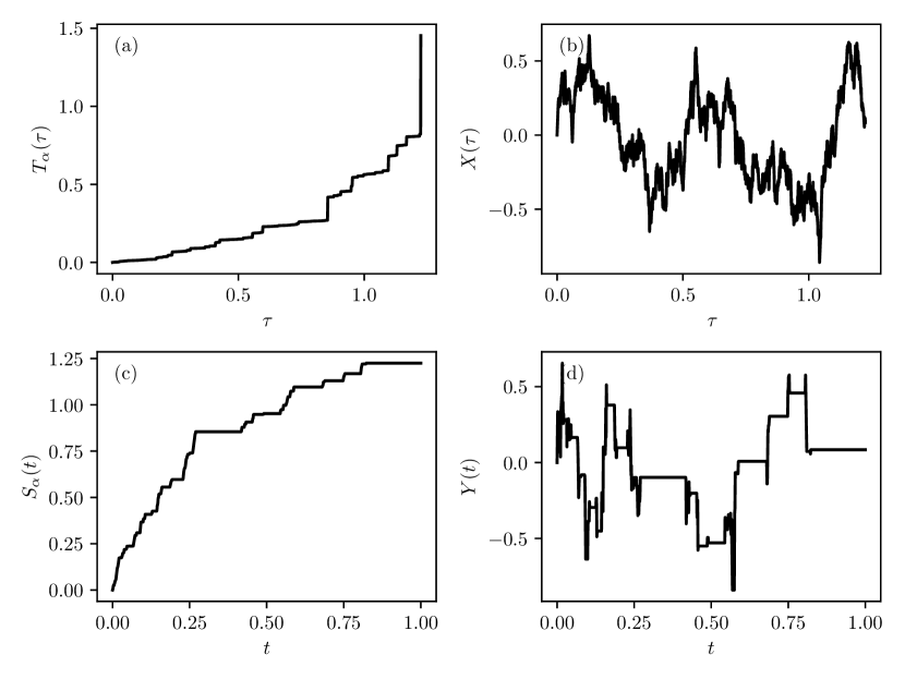
Figure 1: A set of trajectories for the four process that leads to subdiffusion, (a) $\alpha$-stable Lévy motion, (b) Brownian motion, (c) inverse $\alpha$-stable subordinator, (d) subdiffusion. (a) and (b) are both in terms of the operational time $\tau$ and (c) and (d) are in terms of the real physical time $t$. These plots were generated using the algorithm in magdziarz2007fractional , where $T_{\alpha}(\tau)$ is simulated to which $S_{\alpha}(t)$ is found using Eq. (9). Then $Y(t)=X(S_{\alpha}(t))$ can be approximated by interpolating $X(\tau)$ for the values of $S_{\alpha}(t)$. One can see that the delays in (c) correspond to periods of waiting in (d).

The probability density of $Y(t)$ written as $W_{\alpha}(x,t|x_{0})$ can be given in terms of $W(x,\tau|x_{0})$ and $g(\tau,t)$ as follows sokolov2000levy ,

$$W_{\alpha}(x,t|x_{0})=\int_{0}^{\infty}W(x,\tau|x_{0})g(\tau,t)d\tau,$$ (13)

due to the independence of $X(\tau)$ and $S_{\alpha}(t)$. By taking the time derivative of both sides of Eq. (13), whilst using Eq. (11) and integrating by parts we find, $\partial_{t}W_{\alpha}(x,t|x_{0})=-{}_{0}D_{t}^{1-\alpha}\Big{\{}[g(\tau,t)W(x,\tau|x_{0})]_{0}^{\infty}-\int_{0}^{\infty}g(\tau,t)\partial_{\tau}W(x,\tau|x_{0})d\tau\Big{\}}$. From Eq. (10) it is clear that $g(\infty,t)=0$ and ${}_{0}D_{t}^{1-\alpha}g(0,t)=\delta(t)$, thus for $t>0$, and using the normal diffusion equation, we recover the fractional diffusion equation (FDE) metzler2000random ; barkai2001fractional ; metzler2004restaurant ,

$$\frac{\partial}{\partial t}W_{\alpha}(x,t|x_{0})=K_{\alpha}\,{}_{0}D_{t}^{1-\alpha}\frac{\partial^{2}}{\partial x^{2}}W_{\alpha}(x,t|x_{0}),$$ (14)

with $K_{\alpha}$ being the generalized diffusion coefficient which has dimensions $[\text{length}]^{2}/[\text{time}]^{\alpha}$.

Now let us consider not only subordinating the Brownian motion but also the functional of Brownian motion, i.e.

$$\mathcal{A}(S_{\alpha}(t))=\int_{0}^{S_{\alpha}(t)}U[X(t^{\prime})]dt^{\prime}.$$ (15)

The joint density, $P_{\alpha}(x,p,t|x_{0})$, where

$$P_{\alpha}(x,p,t|x_{0})=\int_{0}^{\infty}g(\tau,t)P(x,p,\tau|x_{0})d\tau,$$ (16)

will then be governed by a generalized FKE. Using the same arguments as above we have magdziarz2015asymptotic ,

$$\frac{\partial}{\partial t}P_{\alpha}(x,p,t|x_{0})={}_{0}D_{t}^{1-\alpha}\left[K_{\alpha}\frac{\partial^{2}}{\partial x^{2}}-pU(x)\right]P_{\alpha}(x,p,t|x_{0}).$$ (17)

It is then simple to find $P_{\alpha}(x,p,t|x_{0})$ via Eq. (16), since

$$P_{\alpha}(x,p,t|x_{0})=\int_{0}^{\infty}\langle\delta(\tau-S_{\alpha}(t))\rangle P(x,p,\tau|x_{0})d\tau.$$ (18)

Using Eq. (4) and the properties of independence, we have

$$P_{\alpha}(x,p,t|x_{0})=\left\langle\delta(X(S_{\alpha}(t))-x)e^{-p\int_{0}^{S_{\alpha}(t)}U[X(t^{\prime})]dt^{\prime}}\right\rangle_{x_{0}}$$ (19)

$$=\int_{0}^{\infty}e^{-pA}\rho_{\alpha}(x,A,t|x_{0})dA,$$

where $\rho_{\alpha}(x,A,t|x_{0})$ is the joint density of $X(S_{\alpha}(t))$ and $\mathcal{A}(S_{\alpha}(t))$.

We point out the difference of Eq. (17) compared to the fractional FKE, as mentioned in Sec. 1, which is given by turgeman2009fractional ; carmi2010distributions ,

$$\frac{\partial}{\partial t}P_{\alpha}(x,p,t|x_{0})=K_{\alpha}\frac{\partial^{2}}{\partial x^{2}}\mathcal{D}_{t}^{1-\alpha}P_{\alpha}(x,p,t|x_{0})-pU(x)P_{\alpha}(x,p,t|x_{0})$$ (20)

where $\mathcal{D}_{t}^{1-\alpha}$ is the so-called fractional substantial derivative friedrich2006anomalous ,

$$\mathcal{D}_{t}^{1-\alpha}P_{\alpha}(x,p,t|x_{0})=\frac{1}{\Gamma(\alpha)}\left[\frac{\partial}{\partial t}+pU(x)\right]\int_{0}^{t}\frac{e^{-(t-t^{\prime})pU(x)}}{(t-t^{\prime})^{1-\alpha}}P_{\alpha}(x,p,t^{\prime}|x_{0})dt^{\prime}.$$ (21)

Thus the corresponding density, $\rho_{\alpha}(x,A,t|x_{0})$, is then the joint density of $Y(t)$ and $\mathcal{A}_{\alpha}(t)=\int_{0}^{t}U[Y(t^{\prime})]dt^{\prime}$ (compare to Eq. (15)). Thus the functional is of the subdiffusive motion and is not a subordinated quantity, illustrating that Eq. (20) is the natural generalization of the FKE for studying functionals of subdiffusion.

2.3 Subordinated Local Time

The local time of a stochastic process, originally introduced by Lévy levy1940certains , is an important quantity that characterises the fraction of time the process spends at a certain point, $x_{b}$. We will label the local time, $\ell(t)$, which is defined as the functional $\mathcal{A}(t)$ with $U(x)=\delta(x-x_{b})$, therefore

$$\ell(t)=\int_{0}^{t}\delta(X(t^{\prime})-x_{b})dt^{\prime}.$$ (22)

Without loss of generality, moving forward, we take this point to be at the origin, $x_{b}=0$.

Now, let us consider the subordinated local time, $\ell(S_{\alpha}(t))$, we are able to evince the meaning of this quantity, as follows. Returning to the CTRW paradigm (for the subdiffusive case), where the random walker is described by Eq. (6) we introduce the quantity $\mathcal{N}(t)$, which is the number of times the walker visits a region around the origin, $\partial\Omega$, of width $\varepsilon$ ($\varepsilon$ gives the scale of the jump length i.e. $\langle\xi_{i}^{2}\rangle=\varepsilon^{2}$), up to time $t$ it1965diffusion :

$$\mathcal{N}(t)=\sum_{i=0}^{N(t)}\mathbb{I}_{\partial\Omega}(Y_{i}).$$ (23)

In Eq. (23) $Y_{i}$ is given by Eq. (5) and $\mathbb{I}_{\partial\Omega}(Y_{i})$ is the indicator function, i.e $\mathbb{I}_{\partial\Omega}(Y_{i})=1$ if $Y_{i}\in\partial\Omega$ and $0$ otherwise. Now we take a continuum limit such that $Y_{n}\to X(\tau)$ and $N(t)\to S_{\alpha}(t)$ and introduce a scaling of $K_{\alpha}/\varepsilon^{2}$ to make $\mathcal{N}(t)$ dimensionless,

$$\mathcal{N}(t)=\frac{K_{\alpha}}{\varepsilon^{2}}\int_{0}^{S_{\alpha}(t)}\mathbb{I}_{\partial\Omega}(X(s))ds.$$ (24)

Let us then take the diffusive limit, which entails letting $\varepsilon$ vanish, resulting in the indicator function, $\mathbb{I}_{\partial\Omega}(X(s))$, becoming the Dirac-$\delta$ function, then we have

$$\lim_{\varepsilon\to 0}\varepsilon\mathcal{N}(t)=K_{\alpha}\ell(S_{\alpha}(t)).$$ (25)

The limit in Eq. (25) exists due to the recurrent nature of Brownian motion in one dimension such that the number of visits, $\mathcal{N}(t)$, diverges in the diffusive limit and can be understood as the continuous analog of the (scaled) number of times a subdiffusive particle visits a certain point. Note this limit will not hold in higher dimensions, so one would need to consider a bounded domain where $\partial\Omega$ becomes a thin layer at a reflecting boundary grebenkov2019probability ; grebenkov2020paradigm . It is well known that the local time for a normal diffusive particle is the continuous limit of the number of times the particle visits a certain point it1965diffusion . However, due to the long waiting times embedded in the subdiffusive dynamics a particle may spend anomalously long times at a certain point. Thus, the local time for a subdiffusive particle, $\ell_{\alpha}(t)=\int_{0}^{t}\delta(Y(t^{\prime}))dt^{\prime}$, does not correspond to the continuous limit of the number of times the particle visits a point. So, if one only cares about whether the particle has reached a certain point a number of times, and not how long it has spent there, e.g. if an event occurs when the particle reaches that point for every visit, then the quantity of interest is the subordinated local time, Eq. (25), i.e. $\ell(S_{\alpha}(t))=\int_{0}^{S_{\alpha}(t)}\delta(X(t^{\prime}))dt^{\prime}$. Note that $\ell(S_{\alpha}(t))$ has dimensions $[\text{time}]^{\alpha}/[\text{length}]$, so contrary to its name $\ell(S_{\alpha}(t))$ is not actually a time.

3 Reactive Boundaries

3.1 Generalized Feynman-Kac Equation and Reactions

It is well known that the FKE (2) can be interpreted as diffusion with killing or reactions schuss2015brownian , such that the diffusive particle is removed from the system i.e. by being absorbed. Let us say for simplicity that absorption occurs at the origin, thus we take $U(x)=\delta(x)$. We introduce the killing or first reaction time $\mathcal{T}$ and assume the reaction dynamics are subordinated and thus governed by the stochastic clock, $S_{\alpha}(t)$. Then the probability for a subdiffusive particle starting at $x_{0}$ to be killed in the time interval $[t,t+h)$ can be approximated by

$$\mathbb{P}[\mathcal{T}\in[t,t+h)]_{x_{0}}\approx p\left\langle\delta(X(S_{\alpha}(t)))\right\rangle_{x_{0}}(S_{\alpha}(t+h)-S_{\alpha}(t)).$$ (26)

Eq. (26) can be understood as follows. Every time the particle reaches the origin there is a chance that a reaction occurs and the trajectory will be killed. As we are considering the reaction dynamics are occurring according to $S_{\alpha}(t)$, the physical time interval $[t,t+h)$ corresponds to the interval $[S_{\alpha}(t),S_{\alpha}(t+h))$ for the reaction dynamics. So for $h<<1$ one can approximate $\mathbb{P}[\mathcal{T}\in[t,t+h)]_{x_{0}}$ by multiplying the probability the particle is found at the origin at time $t$ having not reacted previously, $\left\langle\delta(X(S_{\alpha}(t)))\right\rangle_{x_{0}}$, by the interval over which the reactions occur, $(S_{\alpha}(t+h)-S_{\alpha}(t))$, and by the Laplace variable in Eq. (19), $p$, which here is considered as the reactivity.

As each reaction event is taken to be independent of each other, the probability the particle has not reacted (survived) up to time t is given by,

$$\mathbb{P}[\mathcal{T}>t]_{x_{0}}=\lim_{h\to 0}\prod_{i=1}^{M}\left[1-p\left\langle\delta(X(S_{\alpha}(t_{i})))\right\rangle_{x_{0}}(S_{\alpha}(t_{i}+h)-S_{\alpha}(t_{i}))\right],$$ (27)

where we have partitioned the interval $[0,t]$ into $0=t_{0}<t_{1}<...<t_{M}=t$, where $h=t_{i+1}-t_{i}$. In the limit we obtain,

$$\mathbb{P}[\mathcal{T}>t]_{x_{0}}=\left\langle\exp\left\{-p\int_{0}^{t}\delta(X(S_{\alpha}(t)))dS_{\alpha}(t)\right\}\right\rangle_{x_{0}}.$$ (28)

Due to the independence between the subdiffusive dynamics and the reaction events, we find that Eq. (19) (for $U(x)=\delta(x)$), can be understood as grebenkov2020paradigm ; bressloff2022diffusion

$$P_{\alpha}(x,p,t|x_{0})dx=\mathbb{P}[X(S_{\alpha}(t))\in[x,x+dx),t<\mathcal{T}]_{x_{0}}.$$ (29)

This shows $P_{\alpha}(x,p,t|x_{0})$ can be interpreted as the probability density of a subdiffusive particle starting at $x_{0}$ to be at a position $x$ whilst having not reacted at the origin. To link Eq. (29) to the joint probability density of the subordinated local time and position, $\rho_{\alpha}(x,l,t|x_{0})$, we use the integral form of $P_{\alpha}(x,p,t|x_{0})$ in Eq. (19) and with $\rho_{\alpha}(x,l,t|x_{0})dx=\partial_{l}\mathbb{P}[X(S_{\alpha}(t))\in[x,x+dx),\ell(S_{\alpha}(t))<l]_{x_{0}}$ we integrate by parts to find

$$P_{\alpha}(x,p,t|x_{0})dx=\int_{0}^{\infty}dlpe^{-pl}\mathbb{P}[X(S_{\alpha}(t))\in[x,x+dx),\ell(S_{\alpha}(t))<l]_{x_{0}}.$$ (30)

Inside the integral we have the probability density of an exponentially distributed random variable, $\hat{l}$, with mean $1/p$, i.e. $\mathbb{P}[\hat{l}\in[l,l+dl)]=pe^{-pl}dl$. So if we replace $pe^{-pl}$ with $\langle\delta(l-\hat{l})\rangle$, we obtain

$$P_{\alpha}(x,p,t|x_{0})dx=\mathbb{P}[X(S_{\alpha}(t))\in[x,x+dx),\ell(S_{\alpha}(t))<\hat{l}]_{x_{0}}.$$ (31)

Therefore, we have shown that the solution of the generalized FKE (17), $P_{\alpha}(x,p,t|x_{0})$, is the probability density of a subdiffusing particle to be found at a position $x$, whilst the subordinated local time has not exceeded the value of an exponentially distributed random variable $\hat{l}$ (see discussion in Sec. 1 and Refs. grebenkov2019probability ; grebenkov2020imperfect ; grebenkov2020paradigm ; bressloff2022diffusion ). As $\ell(S_{\alpha}(t))$ is a monotonically non-decreasing process, the event of $\{\hat{l}>\ell(S_{\alpha}(t))\}$ is equivalent to $\{\mathcal{T}>t\}$. Thus, by comparing Eq. (31) to Eq. (29) we can see how the reaction time, $\mathcal{T}$, is related to the subordinated local time, $\ell(S_{\alpha}(t))$, via

$$\mathcal{T}=\inf\{t>0:\ell(S_{\alpha}(t))>\hat{l}\}.$$ (32)

In other words the reaction time and subordinated local time are intimately linked processes, with the reaction time being determined by the subordinated local time exceeding a certain value.

3.2 Radiation Boundary Condition

In the previous section we have established the connection between reactions and the generalized FKE, here we extend the idea to when the reactions are occurring on a boundary. We consider a CTRW generated by a nearest-neighbour random walk moving on a discrete one-dimensional lattice with sites $0,1,2,...$ and lattice spacing $\varepsilon$ with the waiting time distribution, $\psi(t)$, being heavy-tailed, thus $\psi(t)\simeq\upsilon^{\alpha}/t^{1+\alpha}$, where $\upsilon$ is a temporal scale parameter. The dynamics of the walker may be described by the GME for the occupation probability at lattice site $i$, initially starting from site $j$, $\mathcal{W}_{i,j}(t)$, for $i>0$ the GME is kenkre1973generalized

$$\frac{d\mathcal{W}_{i,j}(t)}{dt}=\int_{0}^{t}dt^{\prime}\Phi(t-t^{\prime})\frac{\mathcal{W}_{i+1,j}(t^{\prime})+\mathcal{W}_{i-1,j}(t^{\prime})-2\mathcal{W}_{i,j}(t^{\prime})}{2},$$ (33)

where the Laplace transform of the memory kernel being, $\widetilde{\Phi}(\epsilon)=\epsilon\widetilde{\psi}(\epsilon)/(1-\widetilde{\psi}(\epsilon))$, here $\epsilon$ is again the Laplace variable. At the site $i=0$, we have

$$\frac{d\mathcal{W}_{0,j}(t)}{dt}=\int_{0}^{t}dt^{\prime}\Phi(t-t^{\prime})\frac{\mathcal{W}_{1,j}(t^{\prime})-\mathcal{W}_{0,j}(t^{\prime})}{2}.$$ (34)

In the presence of a reactive boundary an incident particle at the lattice site $i=0$, has a probability of reacting $1-k$ and a probability of being reflected $k$. This situation can be summarized by the following flux condition,

$$\mathcal{J}_{0,j}^{+}(t)=k\mathcal{J}_{0,j}^{-}(t).$$ (35)

From Eq. (34) we can identify the discrete fluxes in and out of the boundary as $\mathcal{J}^{+}_{0,j}(t)=\int_{0}^{t}dt^{\prime}\Phi(t-t^{\prime})\mathcal{W}_{0,j}(t^{\prime})/2$ and $\mathcal{J}^{-}_{0,j}(t)=\int_{0}^{t}dt^{\prime}\Phi(t-t^{\prime})\mathcal{W}_{1,j}(t^{\prime})/2$, respectively lomholt2007subdiffusion . If we insert these fluxes into Eq. (35), and using the following relation for the total flux, $\mathcal{J}_{0,j}(t)=\mathcal{J}^{+}_{0,j}(t)-\mathcal{J}^{-}_{0,j}(t)$, we obtain

$$\mathcal{J}_{0,j}(t)=\frac{k-1}{2}\int_{0}^{t}dt^{\prime}\Phi(t-t^{\prime})\mathcal{W}_{1,j}(t^{\prime}),$$ (36)

and find the relation in terms of $\mathcal{W}_{0,j}(t)$, as

$$\mathcal{J}_{0,j}(t)=\frac{k-1}{2k}\int_{0}^{t}dt^{\prime}\Phi(t-t^{\prime})\mathcal{W}_{0,j}(t^{\prime}).$$ (37)

Let us now take the diffusive limit, which entails taking the limits $\varepsilon\to 0$ and $\upsilon^{\alpha}\to 0$ barkai2000continuous . This corresponds to $\widetilde{\psi}(\epsilon)\sim 1-(\upsilon\epsilon)^{\alpha}$, so $\widetilde{\Phi}(\epsilon)\sim\upsilon^{-\alpha}\epsilon^{1-\alpha}$ with $\mathcal{W}_{i,j}(t)/\varepsilon\to W_{\alpha}(x,t|x_{0})$ and $\mathcal{J}_{i,j}(t)\to J_{\alpha}(x,t|x_{0})$, where $i\varepsilon\to x$ and $j\varepsilon\to x_{0}$. By taking the Laplace transform of Eq. (37) and inserting $\widetilde{\Phi}(\epsilon)$, we obtain

$$\widetilde{J}_{\alpha}(0,\epsilon|x_{0})=-\lambda_{\alpha}\epsilon^{1-\alpha}\widetilde{W}_{\alpha}(0,\epsilon|x_{0}).$$ (38)

where the flux is defined as $J_{\alpha}(x,t|x_{0})=-K_{\alpha}\,{}_{0}D_{t}^{1-\alpha}\partial_{x}W_{\alpha}(x,t|x_{0})$ (from writing Eq. (14) as a continuity equation, $\partial_{t}W_{\alpha}(x,t)+\partial_{x}J_{\alpha}(x,t)=0$) and

$$\frac{1-k}{k\varepsilon}K_{\alpha}\to\lambda_{\alpha},$$ (39)

with $\varepsilon^{2}/(2\upsilon^{\alpha})\to K_{\alpha}$. Eq. (39) implies that in the diffusive limit one requires $k\to 1$ grebenkov2003spectral , which is a consequence of the number of visits to the origin becoming infinite.

Taking the inverse Laplace transform of Eq. (38), we have

$$J_{\alpha}(0,t|x_{0})=-\lambda_{\alpha}\,{}_{0}D_{t}^{1-\alpha}W_{\alpha}(0,t|x_{0}).$$ (40)

Clearly Eq. (40) is equivalent to the so-called radiation BC weiss1994aspects ; redner2001guide ; grebenkov2010subdiffusion ,

$$K_{\alpha}\frac{\partial W_{\alpha}(x,t|x_{0})}{\partial x}\Big{|}_{x=0}=\lambda_{\alpha}W_{\alpha}(0,t|x_{0}).$$ (41)

The radiation BC (41) describes a reactive boundary such that an incident particle is either absorbed or reflected depending on the reactivity parameter $\lambda_{\alpha}$ which has dimensions $[\text{length}]/[\text{time}]^{\alpha}$, such that $\lambda_{\alpha}=\infty$ represents full absorption and $\lambda_{\alpha}=0$ represents full reflection.

Note that here we have obtained the reactivity parameter, $\lambda_{\alpha}$, derived from a reaction probability principle, whereas previously it had been found using a reaction rate seki2003recombination ; seki2003fractional ; lomholt2007subdiffusion ; eaves2008subdiffusive .

3.3 Connection Between the Generalized Feynman-Kac Equation and the Radiation Boundary Condition

Starting from the limit form of $\lambda_{\alpha}$ in Eq. (39), for small $\varepsilon$ the probability of reflection can be expressed as $k\approx 1/(1+\varepsilon\lambda_{\alpha}/K_{\alpha})$. The probability of visiting the origin $n$ times without a reaction (being reflected) is simply $k^{n}$ since each interaction is independent, but with reference to Sec. 2.3, we know the particle visits the origin a random number of times, $\mathcal{N}(t)$. To find the probability of the particle, which started at $x_{0}$, to have not reacted, we must average over all possible realisations of $\mathcal{N}(t)$, to which we obtain grebenkov2022encounter

$$\mathbb{P}[\mathcal{T}>t]_{x_{0}}=\left\langle k^{\mathcal{N}(t)}\right\rangle_{x_{0}}.$$ (42)

After inserting the expression for $k$ into Eq. (42) and expanding for small $\varepsilon$, we have

$$\mathbb{P}[\mathcal{T}>t]_{x_{0}}\approx\left\langle\exp\left\{-\frac{\varepsilon\mathcal{N}(t)\lambda_{\alpha}}{K_{\alpha}}\right\}\right\rangle_{x_{0}}.$$ (43)

Using Eq. (25), Eq. (43) in the limit $\varepsilon\to 0$ becomes grebenkov2022encounter ,

$$\mathbb{P}[\mathcal{T}>t]_{x_{0}}=\left\langle e^{-\lambda_{\alpha}\ell(S_{\alpha}(t))}\right\rangle_{x_{0}},$$ (44)

which is exactly Eq. (28) with $\lambda_{\alpha}$ in place of $p$. Note that because of the boundary $X(\tau)$ is now reflected Brownian motion, whereas in Sec. 3.1 we did not impose such a restriction.

This implies that the solution to the FDE, (14) with the radiation BC (41) is equivalent to solving the generalized FKE (17) with $U(x)=\delta(x)$ and the reflecting (Neumann) BC, $\lim_{x\to 0}\partial_{x}P_{\alpha}(x,p,t|x_{0})=0$. We can simply verify this by considering the generalized FKE with $U(x)=\delta(x)$,

$$\frac{\partial}{\partial t}P_{\alpha}(x,\lambda_{\alpha},t|x_{0})={}_{0}D_{t}^{1-\alpha}\Big{[}K_{\alpha}\frac{\partial^{2}}{\partial x^{2}}-\lambda_{\alpha}\delta(x)\Big{]}P_{\alpha}(x,\lambda_{\alpha},t|x_{0}),$$ (45)

where we have replaced $p$ with $\lambda_{\alpha}$ as we are looking specifically at the radiation BC. Eq. (45) has been considered before in the specific context of geminate recombination seki2003fractional ; seki2003recombination ; seki2007specific . Integrating both sides of Eq. (45) over the range $[0,\Delta]$ with respect to $x$ and making use of the reflecting BC, gives seki2003fractional

$$\int_{0}^{\Delta}\frac{\partial}{\partial t}P_{\alpha}(x,\lambda_{\alpha},t|x_{0})dx={}_{0}D_{t}^{1-\alpha}\Big{[}K_{\alpha}\frac{\partial P_{\alpha}(x,\lambda_{\alpha},t|x_{0})}{\partial x}\Big{|}_{x=\Delta}$$ (46)

$$-\lambda_{\alpha}P_{\alpha}(0,\lambda_{\alpha},t|x_{0})\Big{]}.$$

By taking $\Delta\to 0$ the left-hand side vanishes and the radiation BC (41) is recovered, showing the equivalent formulations of the problem. We note that it has recently been shown that another equation (not in the FKE form), coming from (normal) diffusion through permeable barriers, satisfies the radiation boundary condition kay2022diffusion with certain conditions. We extend this equation to the subdiffusive case in Appendix A and show how it leads to the radiation BC. This fact further compounds the notion that the reaction dynamics is a subordinated process.

4 First-Reaction Time

4.1 Generalized Feynman-Kac Equation Solution

To study the first-reaction time (FRT) of a subdiffusive particle in the presence of a radiation boundary at the origin, we must find the corresponding probability density, $P_{\alpha}(x,\lambda_{\alpha},t|x_{0})$. As demonstrated in Sec. 3.3 this may be achieved through two equivalent methods, solving the FDE (14) with the radiation BC (41) or solving the generalized FKE (45) with a reflecting BC at the origin. One can appreciate that the latter task is more amenable. Making use of the method of images montroll1979enriched the solution simply follows through knowledge of the Green’s function of Eq. (45), that is the solution of the FDE with a reflecting BC, which is given in the Laplace domain by metzler2000random

$$\widetilde{W}_{\alpha}(x,\epsilon|x_{0})=\frac{e^{-|x-x_{0}|\sqrt{\epsilon^{\alpha}/K_{\alpha}}}+e^{-|x+x_{0}|\sqrt{\epsilon^{\alpha}/K_{\alpha}}}}{2\sqrt{K_{\alpha}\epsilon^{2-\alpha}}}.$$ (47)

$P_{\alpha}(x,\lambda_{\alpha},t|x_{0})$, is then constructed in terms of the Green’s function as,

$$P_{\alpha}(x,\lambda_{\alpha},t|x_{0})=W_{\alpha}(x,t|x_{0})\\ -\lambda_{\alpha}\int_{0}^{t}dt^{\prime}\int_{0}^{\infty}dyW_{\alpha}(x,t-t^{\prime}|y)\delta(y){}_{0}D_{t^{\prime}}^{1-\alpha}P_{\alpha}(y,\lambda_{\alpha},t^{\prime}|x_{0}).$$ (48)

From the defect technique kenkre2021memory Eq. (48) can be written in the Laplace domain as follows szabo1984localized ,

$$\widetilde{P}_{\alpha}(x,\lambda_{\alpha},\epsilon|x_{0})=\widetilde{W}_{\alpha}(x,\epsilon|x_{0})-\widetilde{W}_{\alpha}(x,\epsilon|0)\frac{\widetilde{W}_{\alpha}(0,\epsilon|x_{0})}{\frac{1}{\lambda_{\alpha}\epsilon^{1-\alpha}}+\widetilde{W}_{\alpha}(0,\epsilon|0)}.$$ (49)

Substitution of Eq. (47) into Eq. (49) gives,

$$\widetilde{P}(x,\lambda_{\alpha},\epsilon|x_{0})=\widetilde{W}_{\alpha}(x,\epsilon|x_{0})-\frac{\lambda_{\alpha}e^{-(x+x_{0})\sqrt{\epsilon^{\alpha}/K_{\alpha}}}}{\lambda_{\alpha}\sqrt{K_{\alpha}\epsilon^{2-\alpha}}+K_{\alpha}\epsilon},$$ (50)

which can be readily shown to satisfy the radiation BC at $x=0$.

4.2 First-Reaction Time Probability Density

To find the FRT probability density we first consider the survival probability Eq. (44), i.e. $Q_{\alpha}(t|x_{0})=\mathbb{P}[\mathcal{T}>t]_{x_{0}}$, to which we may write in terms of the survival probability of normal diffusion, $Q(t|x_{0})=\left\langle\exp\{-\lambda\int_{0}^{t}\delta(X(t^{\prime}))dt^{\prime}\}\right\rangle_{x_{0}}$, dienst2007mean

$$Q_{\alpha}(t|x_{0})=\int_{0}^{\infty}g(\tau,t)\left\langle\exp\left\{-\lambda\int_{0}^{\tau}\delta(X(t^{\prime}))dt^{\prime}\right\}\right\rangle_{x_{0}}d\tau.$$ (51)

As the FRT probability density, $\mathcal{F}_{\alpha}(t|x_{0})$, is the density of the reaction times $\mathcal{T}$, it is then related to the survival probability via $\mathcal{F}_{\alpha}(t|x_{0})=-\partial_{t}Q_{\alpha}(t|x_{0})$. After using Eq. (11) we find

$$\mathcal{F}_{\alpha}(t|x_{0})={}_{0}D_{t}^{1-\alpha}\int_{0}^{\infty}\left\langle\exp\left\{-\lambda\int_{0}^{\tau}\delta(X(t^{\prime}))dt^{\prime}\right\}\right\rangle_{x_{0}}\frac{\partial}{\partial\tau}g(\tau,t)d\tau,$$ (52)

which can be integrated by parts leading to

$$\mathcal{F}_{\alpha}(t|x_{0})=\lambda_{\alpha}{}_{0}D_{t}^{1-\alpha}\left\langle\delta(X(S_{\alpha}(t)))e^{-\lambda_{\alpha}\int_{0}^{S_{\alpha}(t)}\delta(X(t^{\prime}))dt^{\prime}}\right\rangle_{x_{0}},$$ (53)

where we have used $g(\tau,t)=\langle\delta(\tau-S_{\alpha}(t))\rangle$. Comparing Eq. (53) to Eq. (19) one can see that the FRT probability density is simply related to $P_{\alpha}(x,\lambda_{\alpha},t|x_{0})$, via

$$\mathcal{F}_{\alpha}(t|x_{0})=\lambda_{\alpha}{}_{0}D_{t}^{1-\alpha}P_{\alpha}(0,\lambda_{\alpha},t|x_{0}).$$ (54)

This relation is obvious from the radiation BC since the FRT probability density is equal to the (negative) flux at the boundary. Then from Eq. (50) we find the Laplace Transform of the FRT density as eaves2008subdiffusive ,

$$\widetilde{\mathcal{F}}_{\alpha}(\epsilon|x_{0})=\frac{\lambda_{\alpha}e^{-x_{0}\sqrt{\epsilon^{\alpha}/K_{\alpha}}}}{\sqrt{K_{\alpha}\epsilon^{\alpha}}+\lambda_{\alpha}}.$$ (55)

Since Eq. (55) is hard to invert directly, we proceed by finding the Mellin transform, $\mathcal{M}\{f(t)\}=\widehat{f}(s)=\int_{0}^{\infty}t^{s-1}f(t)dt$, and then performing the inverse transform wyss1986fractional ; schneider1989fractional (see Appendix B and C). In the end we obtain,

$$\mathcal{F}_{\alpha}(t|x_{0})=\frac{e^{\lambda_{\alpha}x_{0}/K_{\alpha}}}{t}\Bigg{[}\frac{\lambda_{\alpha}t^{\alpha/2}}{\sqrt{K_{\alpha}}}E_{\frac{\alpha}{2},\frac{\alpha}{2}}\left(-\frac{\lambda_{\alpha}t^{\alpha/2}}{\sqrt{K_{\alpha}}}\right)\\ -\sum_{n=0}^{\infty}\frac{(-1)^{n}\gamma\left(n+1,\frac{\lambda_{\alpha}x_{0}}{K_{\alpha}}\right)}{n!\Gamma\left(\frac{-\alpha n}{2}\right)\left(\frac{\lambda_{\alpha}t^{\alpha/2}}{\sqrt{K_{\alpha}}}\right)^{n}}\Bigg{]},$$ (56)

where $\Gamma(z)=\int_{0}^{\infty}t^{z-1}e^{-t}dt$ is the Gamma function abramowitz1964handbook , $\gamma(z,a)=\int_{0}^{a}t^{z-1}e^{-t}dt$ is the lower incomplete Gamma function abramowitz1964handbook and $E_{a,b}(z)$ is the two-parameter Mittag-Leffler function bateman1953higher3 (see Eq. (89)). Using the integral form of the incomplete Gamma function, we may write Eq. (56) in a more compact integral form,

$$\mathcal{F}_{\alpha}(t|x_{0})=\frac{e^{\lambda_{\alpha}x_{0}/K_{\alpha}}}{t}\Bigg{[}\frac{\lambda_{\alpha}t^{\alpha/2}}{\sqrt{K_{\alpha}}}E_{\frac{\alpha}{2},\frac{\alpha}{2}}\left(-\frac{\lambda_{\alpha}t^{\alpha/2}}{\sqrt{K_{\alpha}}}\right)\\ -\int_{0}^{\frac{\lambda_{\alpha}x_{0}}{K_{\alpha}}}e^{-x}\phi\left(-\frac{\alpha}{2},0\mathchar 24635\relax\;\frac{-\sqrt{K_{\alpha}}}{\lambda_{\alpha}t^{\alpha/2}}x\right)dx\Bigg{]},$$ (57)

where $\phi(a,b\mathchar 24635\relax\;z)$ is the Wright function as defined by the series wright1935asymptotic ; wright1940generalized

$$\phi(a,b\mathchar 24635\relax\;z)=\sum_{n=0}^{\infty}\frac{z^{n}}{n!\Gamma(an+b)},$$ (58)

for $a>-1$. From the Eqs. (56) and (57) we can see that if the particle initially starts at the origin we obtain the FRT density in the simple form,

$$\mathcal{F}_{\alpha}(t|0)=\frac{\lambda_{\alpha}}{\sqrt{K_{\alpha}}t^{1-\frac{\alpha}{2}}}E_{\frac{\alpha}{2},\frac{\alpha}{2}}\left(-\frac{\lambda_{\alpha}t^{\alpha/2}}{\sqrt{K_{\alpha}}}\right).$$ (59)

Using the following Laplace transform relationship between the Wright function and the Mittag-Leffler function gorenflo1999analytical ; luchko2019wright ,

$$E_{a,b+a}(-z)=\int_{0}^{\infty}e^{-zx}\phi(-a,b,-x)dx$$ (60)

for $a>0$, then Eq. (57) becomes,

$$\mathcal{F}_{\alpha}(t|x_{0})=\frac{e^{\lambda_{\alpha}x_{0}/K_{\alpha}}}{t}\int_{\frac{\lambda_{\alpha}x_{0}}{K_{\alpha}}}^{\infty}e^{-x}\phi\left(-\frac{\alpha}{2},0\mathchar 24635\relax\;\frac{-\sqrt{K_{\alpha}}}{\lambda_{\alpha}t^{\alpha/2}}x\right)dx.$$ (61)

This form of the FRT in Eq. (61) is useful for verifying the perfectly reacting/absorbing case ($\lambda_{\alpha}\to\infty)$ and the normal diffusion case ($\alpha\to 1$) (see Appendix D and E). Eq. (61) is now used to find the short and long time asymptotic form of the FRT. After a change of variable in the integral in Eq. (61) we use the expression

$$\mathcal{F}_{\alpha}(t|x_{0})=\frac{\lambda_{\alpha}e^{\lambda_{\alpha}x_{0}/K_{\alpha}}}{\sqrt{K_{\alpha}}t^{1-\frac{\alpha}{2}}}\int_{\frac{x_{0}}{\sqrt{K_{\alpha}t^{\alpha}}}}^{\infty}e^{\frac{-\lambda_{\alpha}t^{\alpha/2}y}{\sqrt{K_{\alpha}}}}\phi\left(-\frac{\alpha}{2},0\mathchar 24635\relax\;-y\right)dy,$$ (62)

to find the large $t$ dependence since lower limit of the integral tends to zero. Thus at long times, using Eq. (60), we have the approximate form of $\mathcal{F}_{\alpha}(t|x_{0})$,

$$\mathcal{F}_{\alpha}(t|x_{0})\approx\frac{\lambda_{\alpha}e^{\lambda_{\alpha}x_{0}/K_{\alpha}}}{\sqrt{K_{\alpha}}t^{1-\frac{\alpha}{2}}}E_{\frac{\alpha}{2},\frac{\alpha}{2}}\left(-\frac{\lambda_{\alpha}t^{\alpha/2}}{\sqrt{K_{\alpha}}}\right).$$ (63)

Using the asymptotic form of the Mittag-Leffler function bateman1953higher3 we have the following asymptotic dependence for $t\to\infty$,

$$\mathcal{F}_{\alpha}(t|x_{0})\sim\frac{\alpha\sqrt{K_{\alpha}}e^{\lambda_{\alpha}x_{0}/K_{\alpha}}}{2\lambda_{\alpha}\Gamma(1-\alpha/2)}t^{-1-\alpha/2},$$ (64)

which confirms the $t^{-1-\alpha/2}$ dependence eaves2008subdiffusive as well as that it possesses the same asymptotic dependence as in the perfectly reacting case rangarajan2000anomalous , leading to an infinite mean yuste2004comment .

Similarly we utilise Eq. (62) to study the short time asymptotics of $\mathcal{F}_{\alpha}(t|x_{0})$, we use bateman1953higher3

$$\partial_{z}\phi(a,b\mathchar 24635\relax\;z)=\phi(a,a+b\mathchar 24635\relax\;z)$$ (65)

to integrate by parts giving and using $\lim_{z\to\infty}\phi\left(-\frac{\alpha}{2},\frac{\alpha}{2}\mathchar 24635\relax\;-z\right)=0$ gorenflo1999analytical , we find

$$\mathcal{F}_{\alpha}(t|x_{0})=\frac{\lambda_{\alpha}e^{\lambda_{\alpha}x_{0}/K_{\alpha}}}{\sqrt{K_{\alpha}}t^{1-\frac{\alpha}{2}}}\Bigg{[}e^{-\lambda_{\alpha}x_{0}/K_{\alpha}}\phi\left(-\frac{\alpha}{2},\frac{\alpha}{2}\mathchar 24635\relax\;-\frac{x_{0}}{\sqrt{K_{\alpha}t^{\alpha}}}\right)$$ (66)

$$-\frac{\lambda_{\alpha}t^{\alpha/2}}{\sqrt{K_{\alpha}}}\int_{\frac{x_{0}}{\sqrt{K_{\alpha}t^{\alpha}}}}^{\infty}e^{\frac{-\lambda_{\alpha}t^{\alpha/2}y}{\sqrt{K_{\alpha}}}}\phi\left(-\frac{\alpha}{2},\frac{\alpha}{2}\mathchar 24635\relax\;-y\right)dy\Bigg{]}.$$

For small $t$ we the can disregard the integral on the right-hand side (RHS) of Eq. (66), then using the asymptotic form of $\phi(a,b,-z)$ for $z\to\infty$ wright1940generalized ; paris2016asymptotic , we find $\mathcal{F}_{\alpha}(t|x_{0})$ has the following dependence for $t\to 0$,

$$\mathcal{F}_{\alpha}(t|x_{0})\sim\frac{\alpha x_{0}\lambda_{\alpha}\left(\frac{\alpha x_{0}}{2\sqrt{K_{\alpha}t^{\alpha}}}\right)^{\frac{1}{\alpha-2}}}{2\sqrt{(2-\alpha)\pi}K_{\alpha}t}\exp\left\{\frac{(\alpha-2)}{2}\left(\frac{\alpha}{2}\right)^{\frac{\alpha}{2-\alpha}}\left(\frac{x_{0}}{\sqrt{K_{\alpha}t^{\alpha}}}\right)^{\frac{2}{2-\alpha}}\right\}.$$ (67)

Eq. (67) indicates a short time exponential form for the FRT consistent with the perfectly reacting case rangarajan2000anomalous . We plot $\mathcal{F}_{\alpha}(t|x_{0})$ in Fig. (2) to prove the validity of our analytic results.

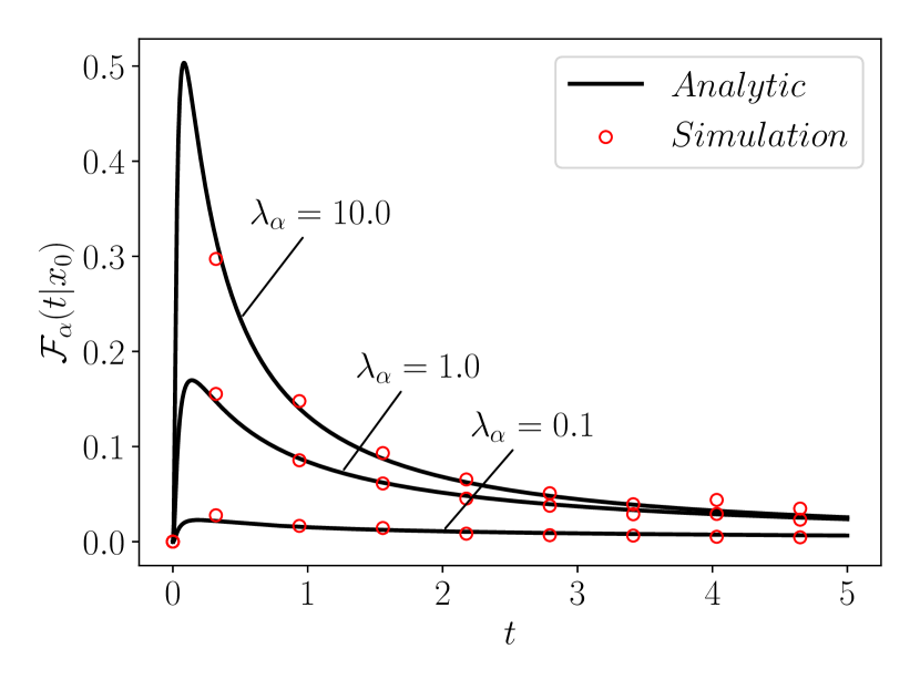
Figure 2: The first-reaction time density, $\mathcal{F}_{\alpha}(t|x_{0})$, Eq. (61) for $\alpha=2/3$, plotted for different values of $\lambda_{\alpha}$, with $x_{0}=2$ and $K_{\alpha}=2$, with all quantities in arbitrary units. We plot these curves against stochastic simulation results (shown as circles), as described in Sec. 4.4.

4.3 Survival Probability and Subordinated Local Time Density

Due to the reaction times, $\mathcal{T}$, being governed by the subordinated local time, $\ell(S_{\alpha}(t))$, we can find the distribution of $\ell(S_{\alpha}(t))$, $\rho_{\alpha}(l,t|x_{0})$, and compare to simulations. From Eq. (44) we know that $\rho_{\alpha}(l,t|x_{0})$ is the inverse Laplace transform of the survival probability $Q_{\alpha}(t|x_{0})$ with respect to $\lambda_{\alpha}$. By finding the survival probability we thus have an easy route to determine the subordinated local time density. We find $Q_{\alpha}(t|x_{0})=\int_{t}^{\infty}\mathcal{F}_{\alpha}(u|x_{0})du$ by using Eq. (61) and Eq. (65) along with the fact that bateman1953higher3

$$az\phi(a,a+b\mathchar 24635\relax\;z)=\phi(a,b-1\mathchar 24635\relax\;z)+(1-b)\phi(a,b\mathchar 24635\relax\;z),$$ (68)

to realize that $t^{-1}\phi\left(-\frac{\alpha}{2},0\mathchar 24635\relax\;\frac{-\sqrt{K_{\alpha}}}{\lambda_{\alpha}t^{\alpha/2}}x\right)=\frac{\partial}{\partial t}\phi\left(-\frac{\alpha}{2},1\mathchar 24635\relax\;\frac{-\sqrt{K_{\alpha}}}{\lambda_{\alpha}t^{\alpha/2}}x\right)$, which gives

$$Q_{\alpha}(t|x_{0})=1-e^{\lambda_{\alpha}x_{0}/K_{\alpha}}\int_{\frac{\lambda_{\alpha}x_{0}}{K_{\alpha}}}^{\infty}e^{-x}\phi\left(-\frac{\alpha}{2},1\mathchar 24635\relax\;\frac{-\sqrt{K_{\alpha}}}{\lambda_{\alpha}t^{\alpha/2}}x\right)dx.$$ (69)

From Eq. (69) we recover the known solutions for the perfectly reactive and normal diffusion cases (see Appendix D and E).

Now we perfrom a change of variable on Eq. (69), which gives

$$Q_{\alpha}(t|x_{0})=1-\int_{0}^{\infty}\lambda_{\alpha}e^{-\lambda_{\alpha}l}\phi\left(-\frac{\alpha}{2},1\mathchar 24635\relax\;-\frac{\sqrt{K_{\alpha}}}{t^{\alpha/2}}(l+x_{0}/K_{\alpha})\right)dl,$$ (70)

after integrating by parts and making use of Eq. (65) this then leads to

$$Q_{\alpha}(t|x_{0})=1-\phi\left(-\frac{\alpha}{2},1\mathchar 24635\relax\;-\frac{x_{0}}{\sqrt{K_{\alpha}t^{\alpha}}}\right)\\ +\frac{\sqrt{K_{\alpha}}}{t^{\alpha/2}}\int_{0}^{\infty}e^{-\lambda_{\alpha}l}\phi\left(-\frac{\alpha}{2},1-\frac{\alpha}{2}\mathchar 24635\relax\;-\frac{\sqrt{K_{\alpha}}}{t^{\alpha/2}}(l+x_{0}/K_{\alpha})\right)dl.$$ (71)

From Eq. (71) the inverse Laplace transform is straightforward and we find the subordinated local time density to be,

$$\rho_{\alpha}(l,t|x_{0})=\delta(l)\left[1-\phi\left(-\frac{\alpha}{2},1\mathchar 24635\relax\;-\frac{x_{0}}{\sqrt{K_{\alpha}t^{\alpha}}}\right)\right]\\ +\frac{\sqrt{K_{\alpha}}}{t^{\alpha/2}}\phi\left(-\frac{\alpha}{2},1-\frac{\alpha}{2}\mathchar 24635\relax\;-\frac{\sqrt{K_{\alpha}}}{t^{\alpha/2}}(l+x_{0}/K_{\alpha})\right).$$ (72)

Clearly for a particle starting at the origin we obtain a simpler expression due to the first term on the RHS of Eq. (72) vanishing.

We are able to find the moments of $\rho_{\alpha}(l,t|x_{0})$, $\langle\ell^{n}(S_{\alpha}(t))\rangle_{x_{0}}=\int_{0}^{\infty}l^{n}\rho_{\alpha}(l,t|x_{0})dl$, from the representation of $Q_{\alpha}(t|x_{0})$ in Eq. (44), where $Q_{\alpha}(t|x_{0})$ can be expressed as the moment generating function of $\ell(S_{\alpha}(t))$, such that

$$Q_{\alpha}(t|x_{0})=\sum_{n=0}^{\infty}\frac{(-1)^{n}}{n!}\lambda_{\alpha}^{n}\langle\ell^{n}(S_{\alpha}(t))\rangle_{x_{0}}.$$ (73)

By repeatedly integrating by parts Eq. (69) whilst using Eq. (65), we are able to express $Q_{\alpha}(t|x_{0})$ as the following infinite series,

$$Q_{\alpha}(t|x_{0})=\sum_{n=0}^{\infty}(-1)^{n}\left(\frac{\lambda_{\alpha}t^{\alpha/2}}{\sqrt{K_{\alpha}}}\right)^{n}\phi\left(-\frac{\alpha}{2},1+\frac{\alpha}{2}n\mathchar 24635\relax\;\frac{-x_{0}}{\sqrt{K_{\alpha}t^{\alpha}}}\right).$$ (74)

Thus we find the moments are uniquely given in terms of Wright functions,

$$\langle\ell^{n}(S_{\alpha}(t))\rangle_{x_{0}}=n!\left(\sqrt{\frac{t^{\alpha}}{K_{\alpha}}}\right)^{n}\phi\left(-\frac{\alpha}{2},1+\frac{\alpha}{2}n\mathchar 24635\relax\;\frac{-x_{0}}{\sqrt{K_{\alpha}t^{\alpha}}}\right).$$ (75)

For $x_{0}=0$ we obtain a simple form for the moments,

$$\langle\ell^{n}(S_{\alpha}(t))\rangle_{0}=\frac{n!}{\Gamma(1+\frac{\alpha}{2}n)}\left(\sqrt{\frac{t^{\alpha}}{K_{\alpha}}}\right)^{n},$$ (76)

which can be realised by using the series form of the Mittag-Leffler function in Eq. (59).

Interestingly, for the specific value of $\alpha=2/3$ gorenflo1999analytical , we find the subordinated local time density to be in terms of the Airy function, $\mbox{Ai}(z)=\frac{1}{\pi}\int_{0}^{\infty}\cos(\frac{t^{3}}{3}+zt)dt$ for $\Im(z)=0$ bateman1953higher2 ,

$$\rho_{2/3}(l,t|0)=3^{2/3}\sqrt{\frac{K_{2/3}}{t^{2/3}}}\mbox{Ai}\left(\sqrt{\frac{K_{2/3}}{(3t)^{2/3}}}l\right).$$ (77)

For $\alpha=1$, one can see that Eq. (72) reduces to the well known Gaussian solution (see Appendix E). In Figure (3), Eq. (77) is utilised to show the correct method of simulating the subordinated local time, as described in the next section.

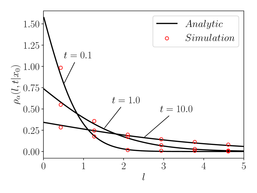
Figure 3: The subordinated local time density, $\mathcal{\rho}_{\alpha}(l,t|x_{0})$, Eq. (77) for $\alpha=2/3$, plotted for different values of $t$, with $x_{0}=0$ and $K_{\alpha}=1$, with all quantities in arbitrary units. We plot these lines against stochastic simulations (shown as circles) of the subordinated local time, as described in Sec. 4.4.

4.4 Simulations

Due to the complexity of our analytic results it is important to validate with numerical simulations. A common method for simulating subdiffusion is through the CTRW formalism in the diffusive limit with a heavy-tailed waiting time distribution, however by keeping in the theme of this work we generate our simulations using a subordinated approach magdziarz2007fractional , as described in Fig. (1). Alternatively, one can simulate the subdiffusion trajectories via the algorithm in Ref. kleinhans2007continuous , which differs from Ref. magdziarz2007fractional through not needing to explicity calculate $S_{\alpha}(t)$. The aforementioned subordinated approach lends naturally to the simulation of the subordinated local time. We are able to effectively approximate, $\ell(S_{\alpha}(t))$ via the discrete construction in Sec. 2.3, where we approximate the limit in Eq. (25) for $\varepsilon<<1$. We approximate the integral in Eq. (24) by writing it in Riemann-Stieltjes form and using the left sided Riemann summation approximation, i.e. by discretizing the time interval, $[0,t]$, as $0=t_{0}<t_{1}<...<t_{M}=t$, then

$$\ell(S_{\alpha}(t))\approx\frac{1}{\varepsilon}\sum_{i=0}^{M-1}\mathbb{I}_{\partial\Omega}(Y(t_{i}))[S_{\alpha}(t_{i+1})-S_{\alpha}(t_{i})].$$ (78)

As we are considering a bounded domain, the subdiffusive trajectories are made to be reflected at the origin. As pointed out in Ref. grebenkov2019probability one must ensure $\varepsilon>>\sqrt{2K_{\alpha}\Delta t}$, where $\Delta t=t/M$, such that the characteristic size of the jump length is not larger than the region $\partial\Omega$, but the smaller the value of $\varepsilon$ the better the approximation of the subordinated local time. The simulation for the FRT density naturally follows from the subordinated local time, where for each trajectory we draw a random number from an exponential distribution with mean $1/\lambda_{\alpha}$ and record the FRT when the subordinated local time exceeds the value of the random number. Given the good match between simulations and theory in Figs. (2) and (3) this provides validation for the analytic results presented.

5 Summary and Conclusions

In summary we have derived, through subordination techniques, a type of generalized FKE and used such an equation to understand and analyse subdiffusion in the presence of a reactive boundary. After deriving the $\alpha$-stable inverse subordinator we perform a time change on the classical FKE to construct a generalized analogue, and find its solution. We introduce the notion of the subordinated local time and we interpret it as the continuum limit of the number of times a subdiffusive particle reaches a given location via a CTRW formulation. An important finding that emerges is that the time spent for each visit does not play a role in the subordinated local time. We apply the formalism to demonstrate how the generalized FKE can be used to describe a subdiffusion process in the presence of reactions. For that we show that the generalized FKE can be thought of as the position density of a subdiffusing particle with the requirement that the subordinated local time is less than a random variable drawn from an exponential distribution with a mean related to the parameter $p$ in the generalized FKE.

We also consider what would be the relevant BC if the reaction occurred on a boundary. We study this aspect by considering a CTRW on a discrete lattice and introduce a reflection probability at the origin, $k$, which gives a general flux condition. From this condition we take the relevant limits to obtain the generalized form of the radiation BC associated with subdiffusion and find the generalized reactivity parameter, $\lambda_{\alpha}$. We then demonstrate the equivalence between the generalized FKE with a reflecting boundary and the FDE with a radiation boundary.

We employ the generalized FKE to study the FRT of a subdiffusive particle in the presence of a radiation boundary at the origin. We solve the generalized FKE using Green’s function techniques and obtain an analytic solution in the Laplace domain. We then find the relation between the solution of the generalized FKE and the FRT probability density and obtain this quantity in the Laplace domain, which we are able to invert by converting it into a Mellin transform. The FRT probability density is obtained in terms of the Mittag-Leffler function and an infinite series of the lower incomplete Gamma functions or alternatively as an integral involving the Wright function. From this we are able to analyse the short and long time asymptotic form of this density recovering expected dependencies. Due to the fundamental connection between the FRT and subordinated local time, we calculate the subordinated local time density and all its moments. Finally, we show how our analytic results match with simulations, proving the validity of simulating subdiffusion in the presence of a radiation boundary using the subordinated local time approach.

A natural extension to this work would be to consider the subordinated occupation time functional ($U(x)=\mathbb{I}_{\Omega}(x)$, for some spatial region $\Omega$) and how this may be used as in a similar sense as the subordinated local time here to describe subdiffusion with reactions in a certain region, not just at a boundary. Further future directions could include developing the backward version of the generalized FKE considered here to study the density of various other subordinated functionals and look at how they compare to functionals of subdiffusion carmi2010distributions . Clearly functionals dependent on the underlying subdiffusive path like local time, occupation time etc. are certainly going to be different. However, the generalized FKE may be applicable to a class of functionals associated with first-passage times, due to only needing the knowledge of whether the particle has reached a specific point, not how long it has been there.

Acknowledgments

We thank Eli Barkai for useful discussions. This work was carried out using the computational facilities of the Advanced Computing Research Centre, University of Bristol - http://www.bristol.ac.uk/acrc/.

Declarations

Funding

TK and LG acknowledge funding from, respectively, an Engineering and Physical Sciences Research Council (EPSRC) DTP student grant and the Biotechnology and Biological Sciences Research Council (BBSRC) Grant No. BB/T012196/1

Data availability

The datasets generated during and/or analysed during the current study are available from the corresponding author on reasonable request.

Conflicts of interest/Competing interests

The authors have no conflicts of interest to declare that are relevant to the content of this article.

Appendix A Non Feynman-Kac Form of Equation Satisfying Radiation Boundary Condition

We consider the following generalization of the so-called inhomogeneous diffusion equation introduced in Eq. (3) of Ref. kay2022diffusion for subdiffusion,

$$\frac{\partial}{\partial t}P_{\alpha}(x,\lambda_{\alpha},t|x_{0})={}_{0}D_{t}^{1-\alpha}\Big{[}K_{\alpha}\frac{\partial^{2}}{\partial x^{2}}P_{\alpha}(x,\lambda_{\alpha},t|x_{0})$$ (79)

$$-\frac{K_{\alpha}^{2}}{\lambda_{\alpha}}\delta^{\prime}(x)\frac{\partial}{\partial x}P_{\alpha}(x,\lambda_{\alpha},t|x_{0})\big{|}_{x=0}\Big{]}$$

with the absorbing (Dirichlet) BC $P_{\alpha}(0,\lambda_{\alpha},t|x_{0})=0$. Let us integrate Eq. (79), as follows

$$\int_{0}^{\Delta}dx\int dx\frac{\partial}{\partial t}P_{\alpha}(x,\lambda_{\alpha},t|x_{0})=K_{\alpha}\,{}_{0}D_{t}^{1-\alpha}P_{\alpha}(\Delta,\lambda_{\alpha},t|x_{0})$$ (80)

$$-\frac{K_{\alpha}^{2}}{\lambda_{\alpha}}{}_{0}D_{t}^{1-\alpha}\frac{\partial}{\partial x}P_{\alpha}(x,\lambda_{\alpha},t|x_{0})\big{|}_{x=0}.$$

Then in the limit $\Delta\to 0$, Eq. (80) tends to the radiation BC, Eq. (41). Without the inclusion of the absorbing BC, Eq. (79) satisifes the permeable/leather BC tanner1978transient ; powles1992exact , where $\lambda_{\alpha}$ would be interpreted as a permeability.

Appendix B Mellin Transform of First-Reaction Time Density

Here we find the Mellin transform of Eq. (55), this is obtained by using the following relationship between the Laplace transform of a function and the Mellin transform schneider1989fractional , where for an arbitrary function we have

$$\widehat{f}(s)=\frac{1}{\Gamma(1-s)}\int_{0}^{\infty}\epsilon^{-s}\widetilde{f}(\epsilon)d\epsilon.$$ (81)

Then from Eq. (81) with Eq. (55) the Mellin transform is found from the integral,

$$\widehat{\mathcal{F}}_{\alpha}(s|x_{0})=\frac{1}{\Gamma(1-s)}\int_{0}^{\infty}\epsilon^{-s}\frac{Be^{A\epsilon^{\alpha/2}}}{\epsilon^{\alpha/2}+B}d\epsilon,$$ (82)

where for simplicity we have introduced the quantities $A=x_{0}/\sqrt{K_{\alpha}}$ and $B=\lambda_{\alpha}/\sqrt{K_{\alpha}}$. Now let us perform a change of variable for the integral in Eq. (82) such that $u=A\epsilon^{\alpha/2}$, thus

$$\widehat{\mathcal{F}}_{\alpha}(s|x_{0})=\frac{2BA^{\frac{2s-2}{\alpha}+1}}{\alpha\Gamma(1-s)}\int_{0}^{\infty}u^{\frac{2-2s}{\alpha}-1}\frac{e^{-u}}{u+AB}du.$$ (83)

Using a certain integral representation of the upper incomplete Gamma function bateman1953higher2 , $\Gamma(z,a)$,

$$\Gamma(z,a)=\frac{a^{z}e^{-a}}{\Gamma(1-z)}\int_{0}^{\infty}\frac{e^{-x}}{x^{z}(x+a)}dx,$$ (84)

we find the Mellin transform of the FRT density to be,

$$\widehat{\mathcal{F}}_{\alpha}(s|x_{0})=\frac{2e^{AB}B^{\frac{2-2s}{\alpha}}\Gamma\left(\frac{2-2s}{\alpha}\right)\Gamma\left(\frac{2s-2}{\alpha}-1,AB\right)}{\alpha\Gamma(1-s)}.$$ (85)

Appendix C Inverse Mellin Transform of First-Reaction Time Density

Before performing the Mellin inverse transform of Eq. (85) we write the upper incomplete Gamma function as $\Gamma(z,a)=\Gamma(z)-\gamma(z,a)$. So we perform a Mellin inversion on each part separately. Thus for the first part we have,

$$\mathcal{M}^{-1}\left\{2e^{AB}\frac{B^{\frac{2-2s}{\alpha}}\Gamma\left(\frac{2-2s}{\alpha}\right)\Gamma\left(\frac{2s-2}{\alpha}+1\right)}{\alpha\Gamma(1-s)}\right\}\\ =\frac{2B^{2/\alpha}e^{AB}}{\alpha 2\pi i}\int_{c-i\infty}^{c+i\infty}\frac{\Gamma\left(\frac{2-2s}{\alpha}\right)\Gamma\left(\frac{2s-2}{\alpha}+1\right)}{\Gamma(1-s)}(B^{\frac{2}{\alpha}}t)^{-s}ds,$$ (86)

with $A$ and $B$ as defined in Appendix B. Here $c$ is a real number lying in a strip where the Mellin transformed function is analytic and tends uniformly to zero as $\Im(s)\to\pm\infty$ kochubei2019handbook . Due to the poles of $\Gamma(z)$ being located at $-n$ for $n=0,1,2,...$, then we can see the poles of the integrand of Eq. (86) are located at $s=1+n\alpha/2$ and $s=1-(n+1)\alpha/2$, so $1-\alpha/2<c<1+\alpha/2$. Due to the integrand diverging for $s\to\infty$, to perform the integral in Eq. (86), we consider the contour $\mathcal{C}=\mathcal{C}_{1}+\mathcal{C}_{2}+\mathcal{C}_{3}+\mathcal{C}_{4}$ shown in Fig. (4). For $R\to\infty$, one can see that contributions from $\mathcal{C}_{2},\mathcal{C}_{3},\mathcal{C}_{4}$ vanish and thus computing the contour, $\mathcal{C}$, integral is equivalent to performing the inverse Mellin transform in Eq. (86). Then from Cauchy’s residue theorem, we only need to compute the residues at the poles, $s=1-(n+1)\alpha/2$.

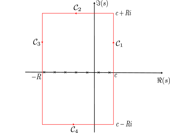
Figure 4: Contour, $\mathcal{C}=\mathcal{C}_{1}+\mathcal{C}_{2}+\mathcal{C}_{3}+\mathcal{C}_{4}$, for the inverse Mellin transform in Eq. (86). The crosses indicate poles.

Using $\mbox{Res}(\Gamma(z),-n)=(-1)^{n}/n!$, we then find the residues to be

$$\mbox{Res}\Bigg{(}\frac{\Gamma\left(\frac{2-2s}{\alpha}\right)\Gamma\left(\frac{2s-2}{\alpha}+1\right)}{\Gamma(1-s)}(B^{2/\alpha}t)^{-s},s=1-\frac{(n+1)\alpha}{2}\Bigg{)}$$ (87)

$$=\frac{\alpha(-1)^{n}(B^{2/\alpha}t)^{\frac{\alpha+\alpha n}{2}-1}}{2\Gamma\left(\frac{\alpha+\alpha n}{2}\right)},$$

leading to

$$\mathcal{M}^{-1}\left\{2e^{AB}\frac{B^{\frac{2-2s}{\alpha}}\Gamma\left(\frac{2-2s}{\alpha}\right)\Gamma\left(\frac{2s-2}{\alpha}+1\right)}{\alpha\Gamma(1-s)}\right\}=\frac{Be^{AB}}{t^{1-\alpha/2}}\sum_{n=0}^{\infty}\frac{(-Bt^{\alpha/2})^{n}}{\Gamma\left(\frac{\alpha+\alpha n}{2}\right)}.$$ (88)

From the series representation of the Mittag-Leffler function bateman1953higher3 ,

$$E_{a,b}(z)=\sum_{n=0}^{\infty}\frac{z^{n}}{\Gamma(an+b)},$$ (89)

one obtains the first term on the RHS of Eq. (56) in the main text.

Now for the other part of Eq. (85) we first decompose the lower incomplete Gamma function into $\gamma(z,a)=a^{z}\Gamma(z)\gamma^{*}(z,a)$, where $\gamma^{*}(z,a)$ is an entire function abramowitz1964handbook . Thus the inverse Mellin transform is computed via,

$$\mathcal{M}^{-1}\left\{2e^{AB}\frac{B^{\frac{2-2s}{\alpha}}\Gamma\left(\frac{2-2s}{\alpha}\right)\gamma\left(\frac{2s-2}{\alpha}+1,AB\right)}{\alpha\Gamma(1-s)}\right\}=\frac{2A^{1-2/\alpha}Be^{AB}}{\alpha 2\pi i}$$

$$\times\int_{c-i\infty}^{c+i\infty}\frac{\Gamma\left(\frac{2-2s}{\alpha}\right)\Gamma\left(\frac{2s-2}{\alpha}+1\right)\gamma^{*}\left(\frac{2s-2}{\alpha}+1,AB\right)}{\Gamma(1-s)}(A^{-\frac{2}{\alpha}}t)^{-s}ds,$$ (90)

so we can see the integrand has the same poles as previously and again $1-\alpha/2<c<1+\alpha/2$. However, due to the the integrand diverging for $s\to-\infty$ we perform the inverse Mellin transform in Eq. (C) using the contour $\mathcal{C}=\mathcal{C}_{1}+\mathcal{C}_{2}+\mathcal{C}_{3}+\mathcal{C}_{4}$ shown in Fig. (5). Again we take $R\to\infty$ and the contributions from $\mathcal{C}_{2},\mathcal{C}_{3},\mathcal{C}_{4}$ vanish, meaning the inverse Mellin transform is computed by finding the residues at the poles $s=1+n\alpha/2$. So the residues are,

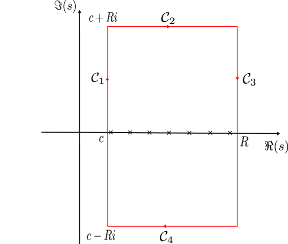
Figure 5: Contour, $\mathcal{C}=\mathcal{C}_{1}+\mathcal{C}_{2}+\mathcal{C}_{3}+\mathcal{C}_{4}$ for the inverse Mellin transform in Eq. (C). The crosses indicate poles.

$$\mbox{Res}\Bigg{(}\frac{\Gamma\left(\frac{2-2s}{\alpha}\right)\Gamma\left(\frac{2s-2}{\alpha}+1\right)\gamma^{*}\left(\frac{2s-2}{\alpha}+1,AB\right)}{\Gamma(1-s)}(A^{-2/\alpha}t)^{-s},s=1+\frac{n\alpha}{2}\Bigg{)}\\ =\frac{\alpha(-1)^{n+1}(A^{-2/\alpha}t)^{\frac{-\alpha n}{2}-1}}{2\Gamma\left(\frac{-\alpha n}{2}\right)}\gamma^{*}(n+1,AB).$$ (91)

Then we find the Mellin transform to be,

$$\mathcal{M}^{-1}\left\{2e^{AB}\frac{B^{\frac{2-2s}{\alpha}}\Gamma\left(\frac{2-2s}{\alpha}\right)\gamma\left(\frac{2s-2}{\alpha}+1,AB\right)}{\alpha\Gamma(1-s)}\right\}\\ =\frac{ABe^{AB}}{t}\sum_{n=0}^{\infty}\frac{(-1)^{n}(At^{-\alpha/2})^{n}\gamma^{*}(n+1,AB)}{\Gamma\left(\frac{-\alpha n}{2}\right)},$$ (92)

then after writing back in terms of $\gamma(z,a)$ we recover the summation in Eq. (56). Note this sum should start from $n=1$ due $1/\Gamma(0)=0$ for $n=0$, but we leave it in this form for easier relation to the Wright function.

Appendix D Perfectly Reactive Case of First-Reaction Time Density and Survival Probability

We start from Eq. (61) and make the change of variable, $y=x-AB$, with $A$ and $B$ as defined in Appendix B, which gives

$$\mathcal{F}_{\alpha}(t|x_{0})=t^{-1}\int_{0}^{\infty}e^{-y}\phi\left(-\frac{\alpha}{2},0\mathchar 24635\relax\;-\frac{y}{Bt^{\alpha/2}}-\frac{A}{t^{\alpha/2}}\right)dx.$$ (93)

Now we take the perfectly reactive limit, $B\to\infty$, which after taking this inside the integral gives,

$$\mathcal{F}_{\alpha}(t|x_{0})=t^{-1}\phi\left(-\frac{\alpha}{2},0\mathchar 24635\relax\;-\frac{A}{t^{\alpha/2}}\right).$$ (94)

Then by using Eq. (68), Eq. (94) becomes

$$\mathcal{F}_{\alpha}(t|x_{0})=\frac{\alpha A}{2t^{1+\alpha/2}}\phi\left(-\frac{\alpha}{2},1-\frac{\alpha}{2}\mathchar 24635\relax\;-\frac{A}{t^{\alpha/2}}\right),$$ (95)

which is the exact solution found in rangarajan2000anomalous . Using the relationship kochubei2019handbook between the Wright function and the Fox H function fox1961G ; mathai1978h ; mathai2009h , $\mathcal{F}_{\alpha}(t|x_{0})$ is found in terms of the very general Fox H function rangarajan2000anomalous

$$\mathcal{F}_{\alpha}(t|x_{0})=\frac{\alpha A}{2t^{1+\alpha/2}}H_{1,1}^{1,0}\left(\frac{A}{t^{\alpha/2}}\Bigg{|}\begin{array}[]{c}(1-\alpha/2,\alpha/2)\\ (0,1)\end{array}\right).$$ (98)

Performing the same change of variables for the survival probability, Eq. (69), and taking the limit $B\to\infty$ we have,

$$Q_{\alpha}(t|x_{0})=1-\phi\left(-\frac{\alpha}{2},1\mathchar 24635\relax\;-\frac{A}{t^{\alpha/2}}\right)$$ (99)

which in terms of the Fox H function we have the known solution yuste2007subdiffusive ,

$$Q_{\alpha}(t|x_{0})=1-H_{1,1}^{1,0}\left(\frac{A}{t^{\alpha/2}}\Bigg{|}\begin{array}[]{c}(1,\alpha/2)\\ (0,1)\end{array}\right).$$ (102)

Note, Eq. (99) appears in the expression for the subordinated local time density, showing the close relationship between the two quantities.

Appendix E Normal Diffusion Case of First-Reaction Time Density, Survival Probability and Subordinated Local Time Density

For $\alpha=1$ we have the following specific value of the Wright function gorenflo1999analytical ,

$$\phi\left(-\frac{1}{2},0\mathchar 24635\relax\;z\right)=-\frac{z}{2\sqrt{\pi}}e^{-z^{2}/4},$$ (103)

then inserting into Eq. (61) we have

$$\mathcal{F}(t|x_{0})=\frac{e^{AB}}{B\sqrt{4\pi t^{3}}}\int_{AB}^{\infty}e^{-x}xe^{-\frac{x^{2}}{4B^{2}t}}dx$$ (104)

with $A$ and $B$ defined in Appendix B. Then we find the FRT for normal diffusion to be

$$\mathcal{F}(t|x_{0})=\frac{Be^{-\frac{A^{2}}{4t}}}{\sqrt{\pi t}}-B^{2}e^{B(A+Bt)}\mbox{erfc}\left(\frac{A+2Bt}{2\sqrt{t}}\right),$$ (105)

where $\mbox{erfc}(z)=1-2\pi^{-1/2}\int_{0}^{z}e^{-t^{2}}dt$ is the complementary error function abramowitz1964handbook . Eq. (105) can easily be found by performing a Laplace transform of Eq. (55) for $\alpha=1$. One may take the limit $B\to\infty$ to find this quantity for normal diffusion with a perfectly reactive boundary, after taking the limit we find the well known result redner2001guide ,

$$\mathcal{F}(t|x_{0})=\frac{A}{\sqrt{4\pi t^{3}}}e^{-\frac{A^{2}}{4t}},$$ (106)

this is also obtained by taking $\alpha\to 1$ in Eq. (98).

Performing a similar procedure for the survival probability, Eq. (69) we find the known solution redner2001guide ,

$$Q(t|x_{0})=e^{B(A+Bt)}\mbox{erfc}\left(\frac{A+2Bt}{2\sqrt{t}}\right)+\mbox{erf}\left(\frac{A}{2\sqrt{t}}\right).$$ (107)

Taking the negative of the time derivative of Eq. (107) we recover Eq.(105) as required. One can see that for $B\to\infty$ we obtain the correct solution for a perfectly reactive boundary.

For the case of $\alpha=1$ for the subordinated local time density, we need to use the following relation gorenflo1999analytical ,

$$\phi\left(-\frac{1}{2},\frac{1}{2}\mathchar 24635\relax\;z\right)=\frac{1}{\sqrt{\pi}}e^{-z^{2}/4},$$ (108)

which from Eq. (72) we recover the following result takacs1995local ,

$$\rho(l,t|0)=\sqrt{\frac{K}{\pi t}}e^{-\frac{K}{4t}l^{2}}.$$ (109)

References

- \bibcommenthead
- (1) R. Metzler, J. Klafter, The random walk’s guide to anomalous diffusion: a fractional dynamics approach. Phys. Rep. 339(1), 1–77 (2000)
- (2) R. Metzler, J. Klafter, The restaurant at the end of the random walk: recent developments in the description of anomalous transport by fractional dynamics. J. Phys. A 37(31), R161 (2004)
- (3) R. Metzler, E. Barkai, J. Klafter, Deriving fractional Fokker-Planck equations from a generalised master equation. EPL 46(4), 431 (1999)
- (4) E. Barkai, R. Metzler, J. Klafter, From continuous time random walks to the fractional Fokker-Planck equation. Phys. Rev. E 61(1), 132 (2000)
- (5) L. Giuggioli, F.J. Sevilla, V. Kenkre, A generalized master equation approach to modelling anomalous transport in animal movement. J. Phys. A 42(43), 434,004 (2009)
- (6) H.C. Fogedby, Langevin equations for continuous time Lévy flights. Phys. Rev. E 50(2), 1657 (1994)
- (7) S.N. Majumdar, in The Legacy Of Albert Einstein: A Collection of Essays in Celebration of the Year of Physics (World Scientific, 2007), pp. 93–129
- (8) L. Turgeman, S. Carmi, E. Barkai, Fractional Feynman-Kac equation for non-Brownian functionals. Phys. Rev. Lett. 103(19), 190,201 (2009)
- (9) S. Carmi, L. Turgeman, E. Barkai, On distributions of functionals of anomalous diffusion paths. J. Stat. Phys. 141(6), 1071–1092 (2010)
- (10) S. Carmi, E. Barkai, Fractional Feynman-Kac equation for weak ergodicity breaking. Phys. Rev. E 84(6), 061,104 (2011)
- (11) A. Cairoli, A. Baule, Anomalous processes with general waiting times: Functionals and multipoint structure. Phys. Rev. Lett. 115(11), 110,601 (2015)
- (12) H. Zhang, G.H. Li, M.K. Luo, Fractional feynman-kac equation with space-dependent anomalous exponent. J. Stat. Phys. 152(6), 1194–1206 (2013)
- (13) A. Cairoli, A. Baule, Feynman-Kac equation for anomalous processes with space-and time-dependent forces. J. Phys. A 50(16), 164,002 (2017)
- (14) X. Wu, W. Deng, E. Barkai, Tempered fractional feynman-kac equation: Theory and examples. Phys. Rev. E 93(3), 032,151 (2016)
- (15) W. Wang, W. Deng, Aging feynman-kac equation. J. Phys. A 51(1), 015,001 (2017)
- (16) X. Wang, Y. Chen, W. Deng, Feynman-Kac equation revisited. Phys. Rev. E 98(5), 052,114 (2018)
- (17) R. Hou, W. Deng, Feynman–kac equations for reaction and diffusion processes. J. Phys. A 51(15), 155,001 (2018)
- (18) P. Lévy, Sur certains processus stochastiques homogènes. Compositio Mathematica 7, 283–339 (1940)
- (19) S.N. Majumdar, A. Comtet, Local and occupation time of a particle diffusing in a random medium. Physical review letters 89(6), 060,601 (2002)
- (20) D.S. Grebenkov, Probability distribution of the boundary local time of reflected Brownian motion in Euclidean domains. Phys. Rev. E 100(6), 062,110 (2019)
- (21) D.S. Grebenkov, in Chemical Kinetics: Beyond the Textbook (World Scientific, 2020), pp. 191–219
- (22) D.S. Grebenkov, Paradigm shift in diffusion-mediated surface phenomena. Phys. Rev. Lett. 125(7), 078,102 (2020)
- (23) S. Redner, A guide to first-passage processes (Cambridge university press, 2001)
- (24) A. Szabo, G. Lamm, G.H. Weiss, Localized partial traps in diffusion processes and random walks. J. Stat. Phys. 34(1), 225–238 (1984)
- (25) T. Kay, T.J. McKetterick, L. Giuggioli, The defect technique for partially absorbing and reflecting boundaries: Application to the ornstein–uhlenbeck process. International Journal of Modern Physics B 36(07n08), 2240,011 (2022)
- (26) D.S. Grebenkov, Subdiffusion in a bounded domain with a partially absorbing-reflecting boundary. Phys. Rev. E 81(2), 021,128 (2010)
- (27) M. Magdziarz, R. Schilling, Asymptotic properties of Brownian motion delayed by inverse subordinators. Proc. Am. Math. Soc. 143(10), 4485–4501 (2015)
- (28) C. Bender, M. Bormann, Y.A. Butko, Subordination principle and feynman-kac formulae for generalized time-fractional evolution equations. arXiv preprint arXiv:2202.01655 (2022)
- (29) M. Naber, Time fractional Schrödinger equation. J. Math. Phys. 45(8), 3339–3352 (2004)
- (30) A. Iomin, Fractional-time quantum dynamics. Phys. Rev. E 80(2), 022,103 (2009)
- (31) B.N. Achar, B.T. Yale, J.W. Hanneken, Time fractional Schrodinger equation revisited. Adv. Math. Phys. 2013 (2013)
- (32) S.Ş. Bayın, Time fractional Schrödinger equation: Fox’s H-functions and the effective potential. J. Math. Phys. 54(1), 012,103 (2013)
- (33) M. Kac, On distributions of certain Wiener functionals. Trans. Am. Math. Soc. 65(1), 1–13 (1949)
- (34) M. Kac, in Proceedings of the second Berkeley symposium on mathematical statistics and probability, vol. 2 (University of California Press, 1951), pp. 189–216
- (35) B. Øksendal, Stochastic differential equations (Springer, 2003)
- (36) Z. Schuss, Brownian dynamics at boundaries and interfaces (Springer, 2015)
- (37) E.W. Montroll, G.H. Weiss, Random walks on lattices. II. J. Math. Phys. 6(2), 167–181 (1965)
- (38) G.H. Weiss, Aspects and applications of the random walk (Elsevier Science & Technology, 1994)
- (39) A. Janicki, A. Weron, Simulation and chaotic behavior of alpha-stable stochastic processes (CRC Press, 2021)
- (40) M.M. Meerschaert, D.A. Benson, H.P. Scheffler, B. Baeumer, Stochastic solution of space-time fractional diffusion equations. Phys. Rev. E 65(4), 041,103 (2002)
- (41) A. Piryatinska, A. Saichev, W. Woyczynski, Models of anomalous diffusion: the subdiffusive case. Physica A 349(3-4), 375–420 (2005)
- (42) M. Magdziarz, A. Weron, J. Klafter, Equivalence of the fractional fokker-planck and subordinated langevin equations: the case of a time-dependent force. Phys. Rev. Lett. 101(21), 210,601 (2008)
- (43) A. Baule, R. Friedrich, Joint probability distributions for a class of non-Markovian processes. Phys. Rev. E 71(2), 026,101 (2005)
- (44) I. Podlubny, Fractional differential equations, mathematics in science and engineering (Academic Press, 1999)
- (45) M. Magdziarz, A. Weron, K. Weron, Fractional Fokker-Planck dynamics: Stochastic representation and computer simulation. Phys. Rev. E 75(1), 016,708 (2007)
- (46) I. Sokolov, Lévy flights from a continuous-time process. Phys. Rev. E 63(1), 011,104 (2000)
- (47) E. Barkai, Fractional Fokker-Planck equation, solution, and application. Phys. Rev. E 63(4), 046,118 (2001)
- (48) R. Friedrich, F. Jenko, A. Baule, S. Eule, Anomalous diffusion of inertial, weakly damped particles. Phys. Rev. Lett. 96(23), 230,601 (2006)
- (49) K. Ito, H. McKean, Diffusion processes and their sample paths. Die Grundlehren der Mathematischen Wissenschaften in Einzeldarstellungen 125 (1965)
- (50) P.C. Bressloff, Diffusion-mediated absorption by partially-reactive targets: Brownian functionals and generalized propagators. J. Phys. A 55(20), 205,001 (2022)
- (51) V. Kenkre, E. Montroll, M. Shlesinger, Generalized master equations for continuous-time random walks. J. Stat. Phys. 9(1), 45–50 (1973)
- (52) M.A. Lomholt, I.M. Zaid, R. Metzler, Subdiffusion and weak ergodicity breaking in the presence of a reactive boundary. Phys. Rev. Lett. 98(20), 200,603 (2007)
- (53) D.S. Grebenkov, M. Filoche, B. Sapoval, Spectral properties of the Brownian self-transport operator. Eur. Phys. J. B 36(2), 221–231 (2003)
- (54) K. Seki, M. Wojcik, M. Tachiya, Recombination kinetics in subdiffusive media. Chem. Phys. 119(14), 7525–7533 (2003)
- (55) K. Seki, M. Wojcik, M. Tachiya, Fractional reaction-diffusion equation. J. Chem. Phys. 119(4), 2165–2170 (2003)
- (56) J.D. Eaves, D.R. Reichman, The subdiffusive targeting problem. J. Phys. Chem. B 112(14), 4283–4289 (2008)
- (57) D.S. Grebenkov, An encounter-based approach for restricted diffusion with a gradient drift. J. Phys. A 55(4), 045,203 (2022)
- (58) K. Seki, A. Shushin, M. Wojcik, M. Tachiya, Specific features of the kinetics of fractional-diffusion assisted geminate reactions. J. Phys. Cond. Matter 19(6), 065,117 (2007)
- (59) T. Kay, L. Giuggioli, Diffusion through permeable interfaces: Fundamental equations and their application to first-passage and local time statistics. Phys. Rev. Res. 4(3), L032,039 (2022)
- (60) E.W. Montroll, B. West, On an enriched collection of stochastic processes Fluctuation Phenomena ed EW Montroll and JL Lebowitz (Amsterdam: North-Holland, 1979)
- (61) V.M. Kenkre, Memory Functions, Projection Operators, and the Defect Technique: Some Tools of the Trade for the Condensed Matter Physicist, vol. 982 (Springer Nature, 2021)
- (62) A. Dienst, R. Friedrich, Mean first passage time for a class of non-Markovian processes. Chaos 17(3), 033,104 (2007)
- (63) W. Wyss, The fractional diffusion equation. J. Math. Phys. 27(11), 2782–2785 (1986)
- (64) W.R. Schneider, W. Wyss, Fractional diffusion and wave equations. J. Math. Phys. 30(1), 134–144 (1989)
- (65) M. Abramowitz, I.A. Stegun, Handbook of mathematical functions with formulas, graphs, and mathematical tables, vol. 55 (US Government printing office, 1964)
- (66) H. Bateman, Higher transcendental functions, vol. 3 (McGraw-Hill Book Company, 1953)
- (67) E.M. Wright, The asymptotic expansion of the generalized Bessel function. Proc. London Math. Soc. 2(1), 257–270 (1935)
- (68) E.M. Wright, The generalized Bessel function of order greater than one. The Quarterly Journal of Mathematics (1), 36–48 (1940)
- (69) R. Gorenflo, Y. Luchko, F. Mainardi, Analytical properties and applications of the Wright function. Fract. Calc. Appl. Anal. 2(4), 383–414 (1999)
- (70) Y. Luchko, (De Gruyter Berlin, 2019), pp. 241–268
- (71) G. Rangarajan, M. Ding, Anomalous diffusion and the first passage time problem. Phys. Rev. E 62(1), 120 (2000)
- (72) S. Yuste, K. Lindenberg, Comment on “Mean first-passage time for anomalous diffusion”. Phys. Rev. E 69(3), 033,101 (2004)
- (73) R.B. Paris, V. Vinogradov, Asymptotic and structural properties of special cases of the Wright function arising in probability theory. Lith. Math. J. 56(3), 377–409 (2016)
- (74) H. Bateman, Higher transcendental functions, vol. 2 (McGraw-Hill Book Company, 1953)
- (75) D. Kleinhans, R. Friedrich, Continuous-time random walks: Simulation of continuous trajectories. Physical Review E 76(6), 061,102 (2007)
- (76) J.E. Tanner, Transient diffusion in a system partitioned by permeable barriers. application to NMR measurements with a pulsed field gradient. Chem. Phys. 69(4), 1748–1754 (1978)
- (77) J.G. Powles, M. Mallett, G. Rickayzen, W. Evans, Exact analytic solutions for diffusion impeded by an infinite array of partially permeable barriers. Proc. R. Soc. Lond. A 436(1897), 391–403 (1992)
- (78) A. Kochubei, Y. Luchko, Handbook of Fractional Calculus with Applications. Volume 1: Basic Theory. (De Gruyter Berlin, 2019)
- (79) C. Fox, The G and H functions as symmetrical Fourier kernels. Trans. Am. Math. Soc. 98(3), 395–429 (1961)
- (80) A.M. Mathai, R.K. Saxena, The H-function with applications in statistics and other disciplines (John Wiley & Sons, 1978)
- (81) A.M. Mathai, R.K. Saxena, H.J. Haubold, The H-function: Theory and Applications (Springer Science & Business Media, 2009)
- (82) S.B. Yuste, K. Lindenberg, Subdiffusive target problem: Survival probability. Phys. Rev. E 76(5), 051,114 (2007)
- (83) L. Takács, On the local time of the Brownian motion. Ann. Appl. Probab. pp. 741–756 (1995)