Thermophysical properties of argon gas from improved two-body interaction potential

Abstract

A new ab initio interaction potential for the electronic ground state of the argon dimer has been developed. The new potential uses previously calculated accurate Born–Oppenheimer potential while significantly improving the description of relativistic effects by including the two-electron Darwin and orbit-orbit corrections. Moreover, retardation of the electromagnetic interactions is taken into account in the long-range part of the potential and leading-order quantum electrodynamics correction is calculated. Spectroscopic properties of the argon dimer such as positions of vibrational levels, bond-dissociation energy, and rotational and centrifugal-distortion constants are reported. We show that the inclusion of the two-electron relativistic terms results in a destabilization of the previously discovered weakly bound ninth vibrational state. Finally, thermophysical properties of the argon gas including pressure and acoustic virial coefficients, as well as transport properties – viscosity and thermal conductivity – are evaluated using the new potential. For the thermophysical properties, the obtained ab initio values are somewhat less accurate than the most recent experimental results. However, the opposite is true for the transport properties, where the theoretical results calculated in this work have significantly smaller uncertainties than the data derived from measurements.

I Introduction

Knowledge of accurate thermophysical properties of noble gases is critical for several areas of physics and chemistry and has been the subject of numerous experimental and ab initio studies. For example, reliable values of thermophysical properties such as pressure, acoustic, dielectric, and refractivity virial coefficients, as well as transport properties such as viscosity and thermal conductivity, are needed in the field of metrology Fellmuth et al. (2006); Schmidt et al. (2007); Moldover et al. (2014); Gaiser and Fellmuth (2019); Rourke et al. (2019); Gaiser et al. (2020, 2022). This is especially important for gas thermometry experiments including the constant-volume gas thermometry Fellmuth et al. (2006), the acoustic gas thermometry Moldover et al. (2014), the dielectric-constant gas thermometry Gaiser and Fellmuth (2019), and the refractive-index gas thermometry Rourke et al. (2019).

Many thermophysical properties of noble gases can be calculated using accurate ab initio potentials. In fact, computations for the helium and neon gases show that thermophysical properties obtained from state-of-the-art ab initio potentials and polarizabilities have uncertainties similar to or even smaller than the best experimental data Czachorowski et al. (2020); Hellmann et al. (2021); Lang et al. (2023a, b). As such, they have been utilized for calibration of high-precision experimental equipment Fellmuth et al. (2006); Gaiser and Fellmuth (2019); Gaiser et al. (2022). Since argon represents an economical alternative to the aforementioned noble gases, its thermophysical properties are of special interest. Their calculation from first principles necessitates the development of a reliable Ar₂ potential, which is a challenging problem. Whereas for the lightest noble gas dimer, He₂, theoretical potentials have become more accurate than the empirical ones in the mid-1990s Williams et al. (1996); Korona et al. (1997), for Ar₂ the empirical potentials such as the one developed by Aziz Aziz (1993) have generally been believed to be the most reliable. Until recently, the most accurate ab initio argon dimer potentials have been developed by Jäger et al. Jäger et al. (2009) and Patkowski et al. Patkowski et al. (2005), with the latter being later refined in Ref. Patkowski and Szalewicz (2010). Last but not least, three new empirical potentials have been published in recent years. These are the 2018 potential of Myatt et al. Myatt et al. (2018) based on re-calibrated Morse/long-range model, the 2019 potential of Song and Yang Song and Yang (2019) with modified repulsive part of the Tang–Toennies model Tang and Toennies (1984), and the latest, 2020 potential by Sheng et al. Sheng et al. (2020) where the conformal behavior among two-body potentials of noble gas atoms is exploited.

To meet the current accuracy requirements, ab initio pair potentials for noble gases have to account for effects beyond the non-relativistic electronic Schrödinger equation. In particular, the relativistic effects bring a considerable contribution to the argon-argon interaction. The first calculation of the relativistic correction to the two-body potential for this system were performed by Faas et al. in 2000 Faas et al. (2000). They calculated the contribution of the relativistic effects near the minimum of the potential using the zeroth-order regular approximation (ZORA) to the Dirac equation and the second-order Møller–Plesset method (MP2) for the treatment of correlation effects. More recent studies Jäger et al. (2009); Patkowski and Szalewicz (2010) included relativistic corrections using other approaches. Jäger et al. Jäger et al. (2009) employed the Cowan–Griffin approximation within the first-order perturbation theory Cowan and Griffin (1976), while Patkowski and Szalewicz Patkowski and Szalewicz (2010) used the second-order Douglas–Kroll–Hess (DKH) relativistic Hamiltonian Douglas and Kroll (1974); Hess (1986). As was noted in Ref. Patkowski and Szalewicz (2010), a good agreement was observed between the two methods; for example, in the region near the minimum of the potential the results differed by merely 0.012 cm^-1, i.e., only about 2% of the total relativistic correction. However, both approaches are able to describe only one-electron relativistic effects, while two-electron effects are completely neglected. These terms may have a substantial contribution to the final results; as noted in Ref. Patkowski and Szalewicz (2010), the two-electron terms amount to 11.6% of the one-electron terms for the internuclear distance of $R=3.75$ Å, i.e., near the minimum of the well. Moreover, as the total two-electron correction vanishes slowly with the increasing internuclear distance, as $R^{-4}$ Meath and Hirschfelder (1966), its relative importance is likely to increase for larger distances.

Regarding the comparison to the available experiments, the aforementioned potentials agree with the experimental results within their uncertainty bounds. The empirical potential of Aziz Aziz (1993) predicts the minimum of the well as $-99.553$ cm^-1 at $R=3.757$ Å, while the potentials of Jäger et al. Jäger et al. (2009) and Patkowski and Szalewicz Patkowski and Szalewicz (2010) predict $-99.48$ cm^-1 at $R=3.762$ Å and $-99.351$ cm^-1 at $R=3.762$ Å, respectively. These predictions agree with the spectroscopic result of Herman et al. Herman et al. (1988) which is $-99.2(10)$ cm^-1 at $R=3.761(3)$ Å. It is also worthwhile to compare the spectroscopic parameters of the available ab initio potentials with the experimental data. The most recent experimental determination of the ground-state rotational ($B_{0}$) and centrifugal-distortion ($D_{0}$) constants was performed by Mizuse et al. Mizuse et al. (2022) using the time-resolved Coulomb explosion imagining. Based on the spectroscopic analysis of the first 14 rotational levels, they obtained $B_{0}=0.057611(4)$ cm^-1 and $D_{0}=1.03(2)\times 10^{-6}$ cm^-1. This can be compared with the theoretical results of Jäger et al. Jäger et al. (2009) who reported $B_{0}=0.05760$ cm^-1 without uncertainty estimates, and did not consider $D_{0}$. Mizuse et al. calculated theoretical values of $B_{0}$ and $D_{0}$ for the potential of Ref. Patkowski and Szalewicz (2010) using rotational levels from Ref. Sahraeian and Hadizadeh (2019). They reported values of $B_{0}=0.057589$ cm^-1 and $D_{0}=1.03\times 10^{-6}$ cm^-1.

Recently, the question of how many rotationless vibrational levels are present in the ground state of argon dimer has emerged. Sahraeian and Hadizadeh Sahraeian and Hadizadeh (2019) solved the momentum-space based Lippmann-Schwinger equation to obtain the vibrational states and reported nine bound levels for the potentials from Refs. Patkowski et al. (2005); Patkowski and Szalewicz (2010). This came after the 2016 study of Tennyson et al. Tennyson et al. (2016) based on the potential of Ref. Patkowski and Szalewicz (2010), where eight bound vibrational levels were found using the $R$-matrix theory and a weakly bound ninth state which was assessed as a numerical byproduct. Eight bounds states were also obtained for the empirical potential of Myatt et al. Myatt et al. (2018) using LEVEL program Le Roy (2017) to solve the nuclear Schrödinger equation. Somewhat later, Rivlin et al. Rivlin et al. (2019a) published a new study using a refined $R$-matrix theory Rivlin et al. (2019b) and also observed the ninth bound vibrational level for the potentials of Refs. Patkowski et al. (2005); Patkowski and Szalewicz (2010). Nevertheless, the existence and position of the ninth vibrational state is still unclear. For example, Sahraeian and Hadizadeh Sahraeian and Hadizadeh (2019) predicted the energy of only $0.20186\times 10^{-6}$ cm^-1 for the potential from Ref. Patkowski and Szalewicz (2010), while Rivlin et al. Rivlin et al. (2019a) obtained about $12\times 10^{-6}$ cm^-1 for the same potential.

In this work, we refine the two-body interaction potential of argon by the inclusion of the two-electron relativistic and retardation effects to properly describe the dissociation limit. Moreover, the leading-order quantum electrodynamics effects are taken into account. The rovibrational levels supported by the new potential are calculated to shed a light on the existence of the ninth bound vibrational state. Next, fully quantum calculations of the second pressure and acoustic virial coefficients of argon gas are performed. Other thermophysical properties of gaseous argon, such as viscosity and thermal conductivity, are also rigorously evaluated within the same framework.

II Pair potential for the argon dimer

The data of Patkowski et al. Patkowski et al. (2005); Patkowski and Szalewicz (2010) are currently the most accurate theoretical results for the non-relativistic interaction energy for two argon atoms. Their Born–Oppenheimer (BO) calculations are saturated with respect to both the basis set and electron excitation limits. Substantial improvements to this component of the two-body potential are not feasible for the foreseeable future with current computational resources. For this reason, we reuse the non-relativistic interaction energy calculated in Refs. Patkowski et al. (2005); Patkowski and Szalewicz (2010) obtained for 41 grid points. However, the description of the relativistic corrections can be still substantially improved as the relativistic effects were included in Ref. Patkowski and Szalewicz (2010) using the second-order DKH approach, which entirely neglects the two-electron corrections.

II.1 Relativistic effects

For systems with nuclear charges below $Z\approx 20$, the relativistic effects can be accounted for perturbatively as the expectation value of the Breit-Pauli Hamiltonian calculated with the nonrelativistic wave function Bethe and Salpeter (1957); Pachucki (2004). The Breit-Pauli Hamiltonian for closed-shell systems has the following form

$$\hat{H}_{\mathrm{BP}}=\hat{H}_{\mathrm{mv}}+\hat{H}_{\mathrm{D1}}+\hat{H}_{\mathrm{D2}}+\hat{H}_{\mathrm{oo}}+\hat{H}_{\mathrm{ssc}},$$ (1)

where $\hat{H}_{\mathrm{mv}}$ is the mass-velocity operator

$$\hat{H}_{\mathrm{mv}}=-\frac{\alpha^{2}}{8}\sum_{i}{\bm{p}_{i}}^{4},$$ (2)

$\hat{H}_{\mathrm{D1}}$ and $\hat{H}_{\mathrm{D2}}$ are the one- and two-electron Darwin operators

$$\hat{H}_{\mathrm{D1}} =\alpha^{2}\frac{\pi}{2}\sum_{I}\sum_{i}\,Z_{I}\delta^{3}(\bm{r}_{Ii}),$$ (3)

$$\hat{H}_{\mathrm{D2}} =-\alpha^{2}\pi\sum_{i<j}\delta^{3}(\bm{r}_{ij}),$$ (4)

$\hat{H}_{\mathrm{oo}}$ is the orbit-orbit operator

$$\hat{H}_{\mathrm{oo}}=-\frac{\alpha^{2}}{2}\sum_{i<j}\left[\frac{\bm{p}_{i}\cdot\bm{p}_{j}}{r_{ij}}+\frac{\bm{r}_{ij}\cdot(\bm{r}_{ij}\cdot\bm{p}_{j})\,\bm{p}_{i}}{r_{ij}^{3}}\right],$$ (5)

and $\hat{H}_{\mathrm{ssc}}$ is the spin-spin contact operator

$$\hat{H}_{\mathrm{ssc}}=-\alpha^{2}\frac{8\pi}{3}\sum_{i<j}(\bm{s}_{i}\cdot\bm{s}_{j})\,\delta^{3}(\bm{r}_{ij}).$$ (6)

In Eqs. (2)–(6) the indices $i$ and $j$ run over all electrons in the system, $\bm{r}_{i}$ is the position vector of the $i$-th electron, $\bm{p}_{i}=-\mathrm{i}\nabla_{\bm{r}_{i}}$ is the momentum operator, and $\bm{s}_{i}=1/2\,\bm{\sigma}_{i}$ is the spin operator, where $\bm{\sigma}$ is a vector of Pauli spin matrices. The index $I$ runs over all nuclei with charges $Z_{I}$ located at positions $\bm{r}_{I}$. $\bm{r}_{Ii}=\bm{r}_{i}-\bm{r}_{I}$ and $\bm{r}_{ij}=\bm{r}_{j}-\bm{r}_{i}$ denote interparticle vectors and $\delta\left(\bm{r}\right)$ is the Dirac delta function. The value of the electron spin $g$-factor is fixed and equal to $2$ and $\alpha=1/137.035\,999\,084$ is the fine-structure constant Tiesinga et al. (2021).

Expectation values of the one-electron relativistic operators, $\hat{H}_{\mathrm{mv}}$ and $\hat{H}_{\mathrm{D1}}$, are usually larger in magnitude than the expectation values of the two-electron relativistic operators, $\hat{H}_{\mathrm{D2}}$ and $\hat{H}_{\mathrm{oo}}$, have opposite sign, and cancel each other to a large extent Piszczatowski et al. (2008). Therefore, it is advantageous to consider them always as a sum, introducing the Cowan–Griffin correction Cowan and Griffin (1976) defined as the expectation value of the operator

$$\hat{H}_{\mathrm{CG}}=\hat{H}_{\mathrm{mv}}+\hat{H}_{\mathrm{D1}}.$$ (7)

In the case of electronic closed-shell singlet spin states, such as the ground states of argon dimer and argon atom, expectation values of $\hat{H}_{\mathrm{D2}}$ and $\hat{H}_{\mathrm{ssc}}$ are related by Coriani et al. (2004)

$$\langle\hat{H}_{\mathrm{ssc}}\rangle=-2\langle\hat{H}_{\mathrm{D2}}\rangle.$$ (8)

The total relativistic correction can then be written as

$$E_{\mathrm{rel}}=\langle\hat{H}_{\mathrm{CG}}\rangle-\langle\hat{H}_{\mathrm{D2}}\rangle+\langle\hat{H}_{\mathrm{oo}}\rangle.$$ (9)

Using the supermolecular approach we calculated the relativistic correction to the interaction energy at a given internuclear distance $R$ as

$$V_{\mathrm{rel}}(R)=E_{\mathrm{rel}}^{\mathrm{Ar}_{2}}(R)-2\,E_{\mathrm{rel}}^{\mathrm{Ar}}(R),$$ (10)

where $E_{\mathrm{rel}}^{\mathrm{Ar}_{2}}(R)$ and $E_{\mathrm{rel}}^{\mathrm{Ar}}(R)$ are the relativistic corrections to the energy of dimer and atom, respectively, computed in the dimer-centered basis set Williams et al. (1995). This is equivalent to applying the so-called counterpoise scheme Boys and Bernardi (1970) to remove the basis set superposition error (BSSE), which is a consequence of unphysical lowering of atomic energies due to the presence of basis functions at both sites in calculations for the dimer.

In order to reduce the basis set incompleteness error (BSIE) in our calculations, and to assess the uncertainty of the ab initio data, we employed the Riemann extrapolation scheme introduced in Ref. Lesiuk and Jeziorski (2019) and used in our previous study of helium dimer Czachorowski et al. (2020). The two-point Riemann extrapolation formula reads

$$E_{\infty}=E_{X}+X^{n}(E_{X}-E_{X-1})\big{[}\zeta(n)-\sum_{i=1}^{X}i^{-n}\big{]},$$ (11)

where $\zeta(s)=\sum_{i=1}^{\infty}i^{-s}$ is the Riemann zeta function. The Cowan-Griffin term converges to the basis set limit at the same rate as the BO energy ($n=4$). However, in the case of the two-electron Darwin term we employed $n=2$ according to the analytic results of Kutzelnigg Kutzelnigg (2008) for the helium atom. To calculate the relativistic corrections, we used uncontracted singly-augmented Dunning-type basis sets aug-cc-pV$X$Z for the argon atom Woon and Dunning (1993, 1994) denoted a$X$Z further in the text. An additional set of midbond functions ($3s3p2d2f1g$) was placed in the middle of the argon-argon bond Slavíček et al. (2003); Patkowski and Szalewicz (2010). We initially calculated the relativistic corrections for 33 internuclear distances on the same grid as in Ref. Patkowski and Szalewicz (2010). However, to improve the accuracy of the potential for small distances, four additional points absent in Ref. Patkowski and Szalewicz (2010) were included (1.2 Å, 1.4 Å, 1.6 Å, and 1.8 Å), bringing the total number of distances to 37. All relativistic ab initio calculations of pair potential were performed using the CCSD(T) method as implemented in DALTON programdal (2018); Aidas et al. (2014), and CCSDT calculations of united atomic limits were done in CFOUR programMatthews et al. (2020); Stanton et al.

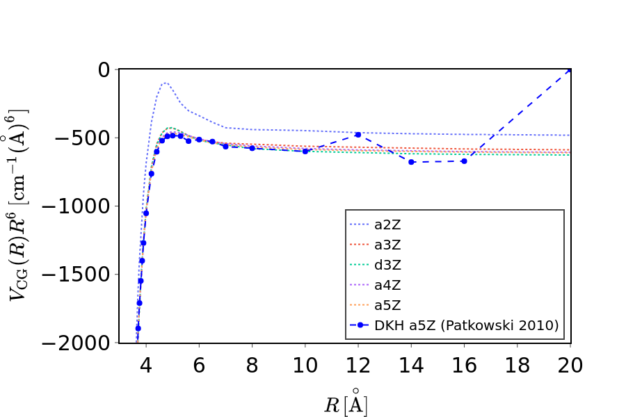
Figure 1: Cowan–Griffin correction to the interaction energy $V_{\mathrm{CG}}(R)$ of the argon dimer as a function of the internuclear distance $R$ calculated using a$X$Z basis sets. For clarity, the results are multiplied by the sixth power of the internuclear distance which corresponds to the leading-order term in the large $R$ asymptotics. The DKH results of Ref. Patkowski and Szalewicz (2010) are given for comparison.

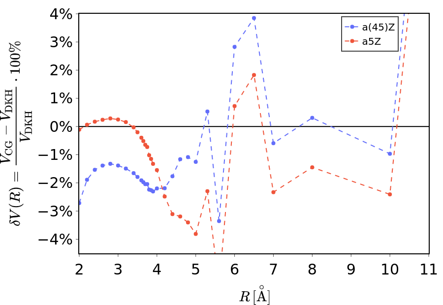
Figure 2: Relative percentage difference between the Cowan–Griffin relativistic correction calculated in this work and the DKH results from Ref. Patkowski and Szalewicz (2010). We compare the data obtained within the a$5$Z basis set (red line), and results obtained by extrapolation from the a(45)Z basis set pair (blue line).

In Fig. 1 we present the Cowan-Griffin contributions to the interaction potential calculated in this work. The DKH results of Patkowski and Szalewicz Patkowski and Szalewicz (2010) are given for comparison. The apparent divergence of the DKH results for large $R$ is a numerical artifact originating from insufficient precision (only one or two significant digits) of the data provided in Ref. Patkowski and Szalewicz (2010). Besides this, a good agreement is observed between the Cowan–Griffin and DKH results for basis sets larger than a2Z. To better illustrate this, in Fig. 2 we show relative difference between the Cowan–Griffin and DKH results from Ref. Patkowski and Szalewicz (2010). On average, the difference is about 2.7% and increases with $R$, but near the minimum of the potential energy curve ($R=3.75$ Å) it amounts to only 0.7% within the a5Z basis set. The final recommended value of the Cowan-Griffin contribution was obtained by the extrapolation from the a(45)Z basis set pair using Eq. (11). For example, at the minimum of the well, the recommended value is $-$0.611 cm^-1.

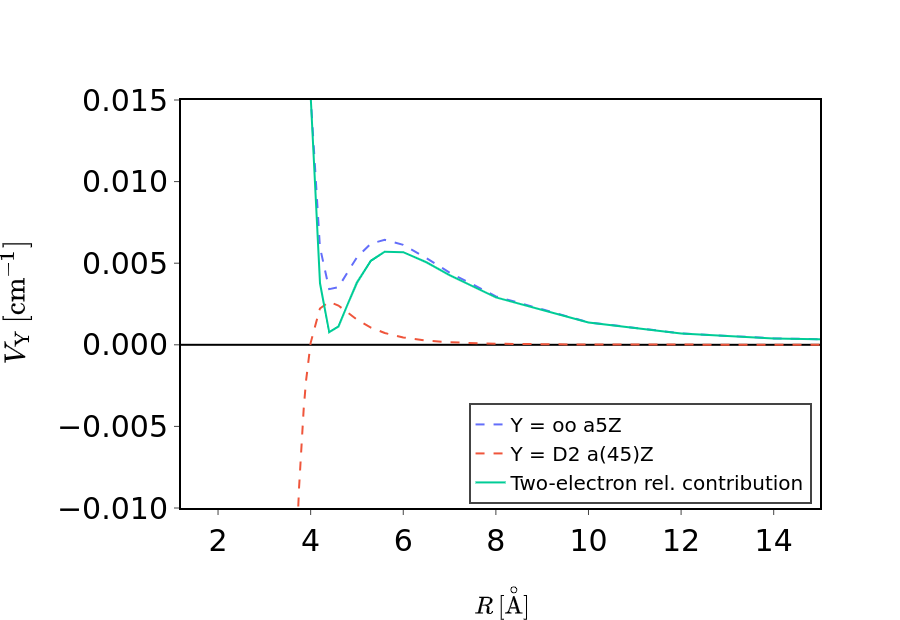
Figure 3: Comparison of two-electron Darwin and orbit-orbit corrections to the interaction energy $V_{\mathrm{Y}}(R)$, $\mathrm{Y}\in\{\mathrm{D2,oo}\}$, of the argon dimer and their total contribution.

In the calculations from Ref. Patkowski and Szalewicz (2010), the two-electron terms in the Breit–Pauli Hamiltonian were neglected and the missing contributions were estimated to be 15% of the one-electron corrections. This estimate was justified by a single calculation of the two-electron Darwin and orbit-orbit terms at $R=3.75$ Å. The total two-electron contribution found by them was roughly $-$0.07 cm^-1 or about 11.6% of the DKH correction. In this work, we explicitly calculated the two-electron terms for all required internuclear distances using a$X$Z basis sets, $X=2-5$. The final results of the two-electron Darwin correction were obtained by extrapolation using Eq. (11) (with $n=2$) from the a$4$Z/a$5$Z basis set pair. Unfortunately, for the orbit-orbit term we encountered non-monotonic convergence behavior with respect to the cardinal number of the basis set which makes the reliability of the extrapolation questionable. Fortunately, the orbit-orbit correction converges rapidly to the basis set limit and the difference between the results obtained within the a$4$Z and a$5$Z basis sets is negligibly small. Therefore, we take the values obtained within a$5$Z basis set as the recommended results for the orbit-orbit correction, and the difference between a$4$Z and a$5$Z results is used as the uncertainty estimate. In Fig. 3 we show the final values of the two-electron Darwin and orbit-orbit corrections to the interaction energy, as well as their sum, as a function of the internuclear distance.

For distances up to $5$ Å, the total two-electron relativistic correction, i.e., the sum of orbit-orbit and two-electron Darwin terms, amounts to between 5% and 12% of the Cowan–Griffin contribution. However, with increasing internuclear distance, the leading $R^{-4}$ term in the asymptotics of the orbit-orbit term starts to dominate. As a result, two-electron terms correspond to about 23% of the Cowan–Griffin contribution at $5.3$ Å, and finally become larger than the latter for $R>7.5$ Å. Finally, our value of two-electron relativistic correction for distance $3.75$ Å  is 0.058 cm^-1, slightly lower than the value of Patkowski and SzalewiczPatkowski and Szalewicz (2010).

II.2 Quantum electrodynamics effects

Another important contribution to the interaction potential originates from the quantum electrodynamics (QED) effects, $E_{\mathrm{QED}}$, of the order of $\alpha^{3}$. In general, the QED correction Caswell and Lepage (1986); Pachucki (1993, 1998) to the energy of atomic and molecular systems consists of one-electron and two-electron components. The former component is given by the expression

$$E_{\mathrm{QED}}=\frac{8\alpha}{3\pi}\Big{(}\frac{19}{30}-2\ln\alpha-\ln k_{0}\Big{)}\langle\hat{H}_{\mathrm{D1}}\rangle,$$ (12)

where $\langle\hat{H}_{\mathrm{D1}}\rangle$ is the relativistic D1 correction as defined in the previous section, and $\ln k_{0}$ is the so-called Bethe logarithm Bethe and Salpeter (1957); Schwartz (1961). The two-electron correction consists of $\langle\hat{H}_{\mathrm{D2}}\rangle$ relativistic term scaled by a small numerical factor, and the so-called Araki-Sucher contribution Araki (1957); Sucher (1958) which is especially difficult to calculate rigorously Balcerzak et al. (2017); Lesiuk et al. (2019); Jaquet and Lesiuk (2020); Czachorowski et al. (2020). The term involving $\langle\hat{H}_{\mathrm{D2}}\rangle$ amounts to less than $0.001\,$cm^-1 for all internuclear distances and hence can be safely neglected. The Araki-Sucher term for the argon dimer was evaluated in Ref. Balcerzak et al. (2017) and is of the order of $0.02\,$cm^-1 for the minimum of the potential. Therefore, the two-electron QED effects are at least by an order of magnitude smaller than the dominant source of the uncertainty in the potential (BO contribution) and are negligible at present.

To determine the one-electron QED correction without additional approximations, one would require the Bethe logarithm, $\ln k_{0}$, for the argon dimer as a function of internuclear distance. Unfortunately, this quantity is unknown at present and we employ the standard approximation of $\ln k_{0}$, taking advantage of its weak dependence on the molecular geometry. Namely, we replace it with the value obtained for the argon atom in Refs. Lesiuk et al. (2020); Lesiuk and Jeziorski (2023)

$$\ln k_{0}=8.7610,$$ (13)

calculated at the Hartree-Fock level of theory.

One may ask whether higher-order QED effects (of the order $\alpha^{4}$ and higher) bring a significant contribution to the potential. To answer this question we evaluated the dominant $\alpha^{4}$ QED contribution for the hydrogen-like atoms, the one-loop term Eides et al. (2001), which reads

$$E_{\mathrm{QED+}}=2\alpha^{2}Z\Big{(}\frac{427}{96}-2\ln 2\Big{)}\langle\hat{H}_{\mathrm{D1}}\rangle$$ (14)

This contribution can be easily obtained from $\langle\hat{H}_{\mathrm{D1}}\rangle$ calculated previously by scaling it with the numerical factor of approximately $0.0059$. Clearly, the higher-order QED contributions are below $0.001\,$cm^-1 for all points of the potential and are negligible within the accuracy requirements of this work. In Table 1 we present a summary of all contributions to the interaction energy of the argon dimer considered in this work for two representative internuclear distances.

Table 1: Contributions to the pair potential of argon at the distance $R=3.75$ Å, i.e., near the minimum of the potential, and $R=7$ Å. The value of the Araki-Sucher term for $R=3.75$ Å was taken from Ref. Balcerzak et al. (2017). The energies are in cm^-1 and the uncertainties at the last digit are given in parentheses.

contribution	value
	$R=3.75$ Å	$R=7$ Å
Born–Oppenheimer	$-98.68(31)$	$-3.0711(79)$
Cowan–Griffin	$-0.602(8)$	$-0.00477(8)$
two-electron Darwin	$-0.0087(1)$	$0.00015(3)$
orbit-orbit	$0.049(5)$	$0.0044(5)$
one-electron QED	$-0.096(1)$	$-0.00242(3)$
two-electron QED	$0.00024(4)$	$-0.0000043(8)$
Araki–Sucher	$0.02$
total	$-99.30(31)$	$-3.0741(79)$

III Fit of the potential

As Patkowski and Szalewicz Patkowski and Szalewicz (2010) fitted only the sum of the BO interaction energy and the DKH correction, we refitted the BO interaction energies alone in order to combine them with the new data. Patkowski and Szalewicz Patkowski and Szalewicz (2010) used a switching function to smoothly connect two separate sets of calculated energies. The first (and more accurate) set for $R>2$ Å was obtained in Ref. Patkowski and Szalewicz (2010) while the second set for 0.25 Å $<R<$ 2 Å was calculated at a lower level of theory in Ref. Patkowski et al. (2005). The switching connects two fitting functions at $R=1.3$ Å Patkowski and Szalewicz (2010). In our work, we fit both sets simultaneously with a global fitting function in the form

$$V_{\mathrm{BO}}(R)=\sum_{i=1}^{2}\sum_{j=-1}^{2}a_{ij}R^{j}\,e^{-\alpha_{i}R}-\sum_{k=3}^{8}\frac{C^{\mathrm{BO}}_{2k}f_{2k+1}(\eta R)}{R^{2k}},$$ (15)

where $f_{n}(x)$ is the Tang–Toennies damping function Tang and Toennies (1984), $a_{ij}$, $\alpha_{i}$, and $\eta$ are fitting parameters and $C^{\mathrm{BO}}_{n}$ are the asymptotic constants. In Ref. Patkowski and Szalewicz (2010), the authors fitted the first two asymptotic constants ($C^{\mathrm{BO}}_{6}$ and $C^{\mathrm{BO}}_{8}$), took $C^{\mathrm{BO}}_{10}$ from Ref. Hättig and Heß (1998), and estimated $C^{\mathrm{BO}}_{12}$, $C^{\mathrm{BO}}_{14}$, and $C^{\mathrm{BO}}_{16}$ from Thakkar’s extrapolation Thakkar (1988), similarly as in Ref. Patkowski et al. (2005). We follow their approach and determine $C^{\mathrm{BO}}_{6}$ and $C^{\mathrm{BO}}_{8}$ by fitting, but employ a more recent and accurate value of $C^{\mathrm{BO}}_{10}=49033$ a.u. from Ref. Jiang et al. (2015). Higher asymptotic constants, $C^{\mathrm{BO}}_{n}$ for $n>10$, were extrapolated from $C^{\mathrm{BO}}_{6}$, $C^{\mathrm{BO}}_{8}$, and $C^{\mathrm{BO}}_{10}$ as in Ref. Jiang et al. (2015) using extrapolation formula from Ref. Thakkar (1988), and were fixed during the fitting.

Due to fact that the $C^{\mathrm{BO}}_{6}$ and $C^{\mathrm{BO}}_{8}$ coefficients are not fixed, a stronger damping is needed in the fitting procedure. In comparison to the previous studies of the argon dimer, we damp the long-range contributions using the Tang-Toennies function $f_{n+1}$ instead of $f_{n}$, where $n$ is the inverse power of internuclear distance in the asymptotic expansion. The reason for this stronger damping is that we force our fit to follow the condition

$$V_{\mathrm{BO}}(R)=\frac{18^{2}}{R}+(E^{\mathrm{Kr}}-2E^{\mathrm{Ar}})+\mathcal{O}(R^{2}),$$ (16)

to ensure the correct short-range asymptotics of the potential. Was this stronger damping not assumed, $C_{n}$ constants would appear in the fitting constraints and severely complicate the fitting procedure. The difference between the ground state energies $(E^{\mathrm{Kr}}-2E^{\mathrm{Ar}})=-1698.4211$ a.u. was calculated using the CCSDT method within the a5Z basis set. The fitted parameters were obtained from 41 ab inito Born-Oppenheimer interaction energies form Refs. Patkowski et al. (2005); Patkowski and Szalewicz (2010).

While the explicit uncertainties of the calculations were reported in Ref. Patkowski and Szalewicz (2010), this is not true for the data from Ref. Patkowski et al. (2005). Therefore, we have assumed a conservative value of 2% for the grid points smaller than 2 Å. We justify our choice by an observation that difference between the extrapolated and unextrapolated data in Ref. Patkowski et al. (2005) was always less that 1.7% for small distances. During the fitting procedure, the adjustable parameters were determined using the non-linear least squares dogbox algorithm Voglis and Lagaris (2004) with weights equal to the squared inverse of the uncertainties. Our final value $C^{\mathrm{BO}}_{6}=64.2295$ a.u. is similar to the result of Patkowski and Szalewicz Patkowski and Szalewicz (2010), $C^{\mathrm{BO}}_{6}=64.2890$ a.u., and the estimate of Kumar and Meath Kumar and Meath (1985), $C^{\mathrm{BO}}_{6}=64.30$ a.u. Only a slightly worse agreement is obtained for the second coefficient, $C^{\mathrm{BO}}_{8}=1503.453$ a.u., in comparison with $C^{\mathrm{BO}}_{8}=1514.86$ a.u. from Ref. Patkowski and Szalewicz (2010) and $C^{\mathrm{BO}}_{8}=1621.5$ a.u. from Ref.Jiang et al. (2015).

In Fig. 4 we show the comparison of absolute errors of the fit with the estimated uncertainties. The mean absolute error (MAE) of the fit is $0.49\,\sigma_{\mathrm{BO}}$, i.e., it is about two times smaller than the inherent uncertainty of the ab initio data points.

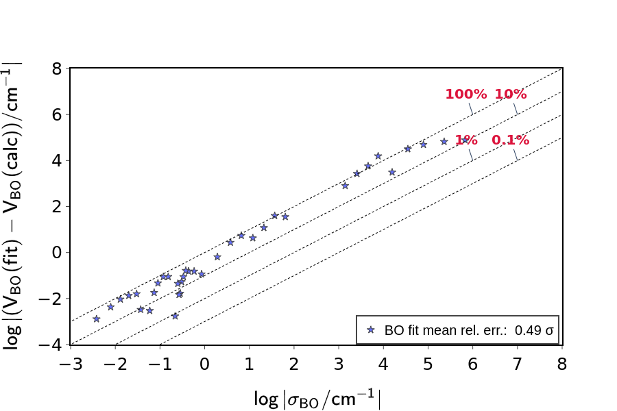
Figure 4: Absolute differences between BO pair potential predicted from the fit, $V_{\mathrm{BO}}(\mathrm{fit})$, and obtained from ab initio calculations, $V_{\mathrm{BO}}(\mathrm{calc})$, versus estimated theoretical uncertainties $\sigma_{\mathrm{BO}}$. The dotted lines and percentage in the legend correspond to relative errors with respect to the estimated uncertainty (1$\sigma_{\mathrm{BO}}=100\%$).

The relativistic corrections to interaction energy were fitted using the formula

$$V_{\mathrm{rel}}(R)=\sum_{i=1}^{2}\sum_{j=0}^{2}a_{ij}R^{j}\,e^{-\alpha_{i}R}-\sum_{k=2}^{4}\frac{C^{\mathrm{rel}}_{2k}f_{2k}(\eta R)}{R^{2k}},$$ (17)

The restriction $V_{\mathrm{rel}}(0)=-31.91275$ a.u. was based on results of the CCSDT calculations using uncontracted aug-cc-pV5Z basis set and enforced during the fit. As no values of the relativistic asymptotic constants have been published published to date, we restricted the asymptotic expansion to $C^{\mathrm{rel}}_{4}$, $C^{\mathrm{rel}}_{6}$, and $C^{\mathrm{rel}}_{8}$ terms to reduce the possibility of over-fitting. All parameters appearing in the above formula were optimized during the fitting procedure. The mean absolute error of our fit is $0.05\,\sigma_{\mathrm{rel}}$, see Fig. 5.

Lastly, we fitted QED effects using a model function

$$\begin{split}V_{\mathrm{QED}}(R)&=(a_{0}+a_{1}R)e^{-\alpha R}+b_{2}R^{2}e^{-\beta R}\\ &-\sum_{k=3}^{4}\frac{C^{\mathrm{QED}}_{2k}f_{2k}(\eta R)}{R^{2k}}.\end{split}$$ (18)

Similarly to the relativistic fit, asymptotic expansion coefficients are not known and hence all parameters were adjusted during the fitting. The final mean absolute error of the QED fit is $0.18\,\sigma_{\mathrm{QED}}$, see Fig. 5. The total interaction potential of the argon dimer, $V(R)$, is calculated as a sum of $V_{\mathrm{BO}}(R)$, $V_{\mathrm{rel}}(R)$, and $V_{\mathrm{QED}}(R)$.

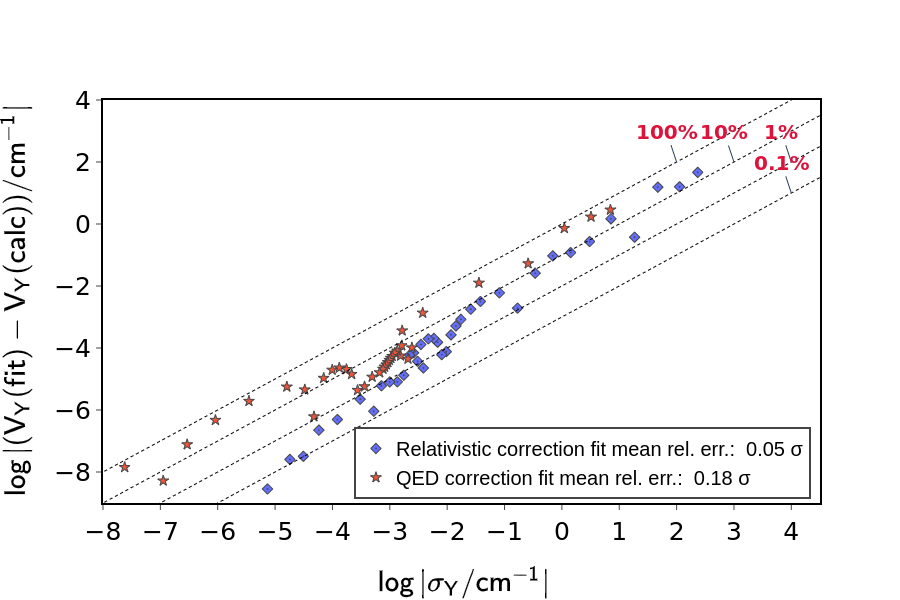
Figure 5: Absolute differences between $\mathrm{Y}\in\{\mathrm{rel},\mathrm{QED}\}$ correction predicted from the fit, $V_{\mathrm{Y}}(\mathrm{fit})$, and obtained from ab initio calculations, $V_{\mathrm{Y}}(\mathrm{calc})$, versus estimated theoretical uncertainties $\sigma_{\mathrm{Y}}$. The dotted lines and percentage in the legend correspond to relative errors with respect to the estimated uncertainty (1$\sigma_{\mathrm{Y}}=100\%$).

In order to estimate the uncertainties of the calculated properties of the argon gas, we generate a fit of $\sigma_{\mathrm{Y}}(R)$, $\mathrm{Y}=\mathrm{BO},\mathrm{rel}$ representing the uncertainties due to errors in the ab initio calculations. As the uncertainty of the QED correction is much smaller than the uncertainty of the relativistic correction we neglect it. The exact value of the potential is expected to be contained within the range $V_{Y}(R)\pm\sigma_{Y}(R)$. Note that the function $\sigma_{\mathrm{Y}}(R)$ is not intended to precisely fit the uncertainties, but rather to follow a general trend as a function of the internuclear distance and provide an upper bound to the calculated uncertainties. The analytical form of $\sigma_{Y}(R)$ reads

$$\sigma_{\mathrm{Y}}(R)=s_{0}e^{-a^{\mathrm{Y}}R}+\sum_{i=1}^{3}s_{i}e^{-a_{i}R^{2}},$$ (19)

where $s_{i}$ and $a_{i}$ are fitting parameters and $a^{\mathrm{Y}}$ were fixed ($a^{\mathrm{BO}}=1.9$ and $a^{\mathrm{rel}}=1.05$) to provide a baseline for the decay of the uncertainty. The fit of the uncertainties was performed using the standard least-squares method applied to a reduced set of data points obtained by discarding points where the values of the uncertainties are significantly smaller than the neighboring ones. The average ratio of the value of $\sigma_{\mathrm{Y}}$ to the uncertainty of the ab initio data was 1.08 for $\sigma_{\mathrm{BO}}$ and 1.17 for $\sigma_{\mathrm{rel}}$ and median 1.16 for both fits. The total uncertainty of the interaction potential is equal to the square root of the sum of squares of $\sigma_{\mathrm{BO}}$ and $\sigma_{\mathrm{rel}}$.

IV Long-range retardation of the potential

In the regime where the internuclear distance is large, retardation of the electromagnetic radiation has to be taken into account. According to the Casimir-Polder theory Casimir and Polder (1948), the dominant effect of the retardation is to switch the usual London’s $R^{-6}$ long-range decay of the interaction energy to the $R^{-7}$ form. To this end, we use the Casimir-Polder formula for the retarded potential

$$U_{\mathrm{CP}}(R)=\frac{\hbar}{\pi R^{6}}\int_{0}^{\infty}[\alpha_{d}(i\omega)]^{2}e^{-2\alpha\omega R}P(\alpha\omega R)d\omega,$$ (20)

where $\alpha_{d}(i\omega)$ is the dipole polarizability of argon atom at an imaginary frequency $i\omega$, $c$ is the speed of light, and $P(x)=x^{4}+2x^{3}+5x^{2}+6x+3$ is a fourth-order polynomial. In this work, we adopted $\alpha_{d}(i\omega)$ calculated in Ref. Jiang et al. (2015) and evaluated $U_{\mathrm{CP}}(R)$ for $100$ internuclear distances within the interval $[0,250]$ bohr. As the direct application of the formula (20) is inconvenient computationally, the follow the approach of Refs. Przybytek et al. (2010, 2012) and use a fitted potential in the form

$$U_{\mathrm{CP}}(R)\approx g(R)\,\frac{C_{6}}{R^{6}},$$ (21)

where $C_{6}=64.30$ corresponds to the BO asymptotic coefficient calculated from the dipole polarizabilities of Ref. Jiang et al. (2015). In the above expression, $g(x)$ is a rational function defined as

$$g(x)=\frac{1+\sum_{n=1}^{5}A_{n}x^{n}}{1+\sum_{n=1}^{6}B_{n}x^{n}},$$ (22)

where $A_{n}$ and $B_{n}$ are the fitting coefficients.

The coefficients $A_{n}$ and $B_{n}$ were obtained by least-squares fitting of Eq. (21) to the aforementioned $100$ data points. To assure the correct long-range behavior in Eq. (21), we used the value of the $C_{6}$ coefficient calculated from the polarizabilities of Ref. Jiang et al. (2015), rather than the value $C_{6}^{\mathrm{BO}}$ obtained by fitting the BO potential as described in the previous section. Furthermore, the value $\alpha_{d}(0)=11.08$ Jiang et al. (2015); Derevianko et al. (2010) was used in determination of the coefficients $A_{5}$ and $A_{6}$, see Eqs. (51-52) in Ref. Cencek et al. (2012). As no reference value for the relativistic asymptotic coefficient $C_{4}$ is available in the literature, we used our value obtained from Eq. (17), see Eqs. (49-50) in Ref. Cencek et al. (2012). Finally, the $C_{3}$ asymptotic coefficient, originating from the Araki-Sucher quantum electrodynamics correction Pachucki (1998), was calculated from the exact expression:

$$C_{3}=\frac{7N_{e}^{2}}{6\pi}\alpha^{3},$$ (23)

where $N_{e}=18$ is number of electrons in the argon atom.

V Spectroscopic parameters

To calculate the spectroscopic and thermophysical properties of argon dimer, one has to solve the radial nuclear Schrödinger equation

$$\Big{[}\frac{d^{2}}{dR^{2}}+2\mu_{A}(E-V(R))-\frac{l(l+1)}{R^{2}}\Big{]}\chi_{l}(r)=0,$$ (24)

where $V(R)$ is the interatomic electronic potential, $l$ is the angular quantum number, and $\chi_{l}$ is the nuclear wave function. While no analytical solution exists, several numerical approaches are available to solve second-order ordinary differential equations such as Eq. 24.

One of the most common techniques is the Numerov integration method Noumerov (1924); Numerov (1927); Blatt (1967), in particular in the renormalized form Johnson (1977). The wave function obtained by the traditional Numerov method can grow exponentially in the classically-forbidden regions which is numerically problematic. However, in the renormalized Numerov method one instead propagates the ratio of the values of the wave function at two consecutive grid points. This ratio is, in practice, bounded and hence the problem of the exponential growth is eliminated. However, this comes at a price of losing the correct normalization of the wave function which must be restored afterwards. Another advantage of the renormalized Numerov method is the direct access to the quantity $\chi^{\prime}(R)/\chi(R)$ required in calculation of phase shifts and thermophysical properties described in the next section.

Using the renormalized Numerov method we calculated bound vibrational states for three potentials reported in this work:

• non-relativistic BO potential with Cowan-Griffin relativistic correction;

• non-relativistic BO potential with full Breit-Pauli relativistic- correction;

• the latter potential with additional QED correction.

The retardation effects were included in the second and third potentials. For comparison, we also provided the corresponding results for two potentials taken from the literature:

• the ab initio potential of Patkowski et al. Patkowski and Szalewicz (2010);

• the latest empirical potential of Song et al.Song and Yang (2019)

The results of the calculations with all potentials are presented in Tab.2.

Table 2: Comparison of the various argon dimer potentials of this work and published literature. Potential constants and energy levels are in cm^-1 and values in parentheses correspond to uncertainty.

Potential	Patkowski 2010	Song 2019	This work			Exp.
(Rel. corr.)	(DKH)	(Empirical)	(Cowan–Griffin)	(full $H_{\mathrm{BP}}$)	(full $H_{\mathrm{BP+QED}}$)
$R_{\epsilon}$ [a.u.]	$3.762$	$3.761$	$3.7634$	$3.7639(14)$	$3.7637(14)$	$3.761(3)$
$D_{\epsilon}$ [cm-1]	$-99.351\textsuperscript{\ref{note:Pat}}$	$-99.60$	$-99.28$	$-99.24(37)$	$-99.33(37)$	$-99.2(10)\textsuperscript{\ref{note:Her}}$
$\nu=0$	$-84.53458$	$-84.40$	$-84.56$	$-84.46(34)$	$-84.55(34)$	$-84.47(1)\textsuperscript{\ref{note:Her}}$
$\nu=1$	$-58.85674\textsuperscript{\ref{note:Sah}}$	$-58.26$	$-58.86$	$-58.83(29)$	$-58.90(29)$	$-58.78(1)\textsuperscript{\ref{note:Her}}$
$\nu=2$	$-38.36106\textsuperscript{\ref{note:Sah}}$	$-37.61$	$-38.35$	$-38.35(24)$	$-38.41(24)$	$-38.2(2)\textsuperscript{\ref{note:Her}}$
$\nu=3$	$-22.85141\textsuperscript{\ref{note:Sah}}$	$-22.18$	$-22.84$	$-22.84(19)$	$-22.88(19)$	$-22.62(2)\textsuperscript{\ref{note:Her}}$
$\nu=4$	$-11.97942\textsuperscript{\ref{note:Sah}}$	$-11.51$	$-11.97$	$-11.96(13)$	$-11.99(13)$	$-11.71(3)\textsuperscript{\ref{note:Her}}$
$\nu=5$	$-5.17193\textsuperscript{\ref{note:Sah}}$	$-4.91$	$-5.17$	$-5.15(8)$	$-5.17(8)$	$-4.87(7)\textsuperscript{\ref{note:Her}}$
$\nu=6$	$-1.59539\textsuperscript{\ref{note:Sah}}$	$-1.48$	$-1.60$	$-1.59(4)$	$-1.60(4)$	-
$\nu=7$	$-0.22722\textsuperscript{\ref{note:Sah}}$	$-0.20$	$-0.23$	$-0.22(1)$	$-0.23(1)$	-
$\nu=8$	$-0.20186\times 10^{-6}$ 3	-	-	-$(-6\times 10^{-6})$	-$(-15\times 10^{-6})$	-
$B_{0}$	0.0575895	0.057580	0.057588	0.057546(45)	0.057553(46)	0.057611(4)
$10^{6}\times D_{0}$ 4	1.035	0.99	1.04	1.04(1)	1.04(1)	1.03(2) 5

We obtained at least eight bound vibrational states with each potential; the ninth bound state was observed only with the potential of Patkowski Patkowski and Szalewicz (2010) and our potential with Cowan-Griffin correction. The addition of the two-electron terms makes the potential more shallow and no ninth bound state was observed. Similarly, no ninth bound state was observed with the empirical potential. As mentioned in the introduction, the ninth bound state of potential of Patkowski was originally deemed as a numerical byproduct Tennyson et al. (2016) and only later confirmed by other studies Rivlin et al. (2019a); Sahraeian and Hadizadeh (2019). Therefore, to ascertain that the disappearance of the ninth vibrational state is not a numerical artifact or an issue with numerical precision, we double-check the results using the Levinson theorem Levinson (1949). According to this theorem, the value of the absolute phase shift $\delta_{l}(E)$ for $E\to 0$ and $l=0$ is equal to the number of bound states supported by the potential times $\pi$. We confirmed that the potentials which supported nine bound states have the absolute phase shifts equal to $9\pi$, while for other potentials the absolute phase shift was $8\pi$. Regarding other spectroscopic parameters, all potentials agree on the location of the minimum of the potential well at $R=7.11\,$Å and its depth, roughly $99.3\,$ cm^-1. Rotational and centrifugal-distortion constants were calculated as well and agree with the experimental values of Ref. Mizuse et al. (2022) within the combined error bars. Overall, the vibrational levels obtained with all potentials are close to the experimental data, with the new potential (including the full Breit-Pauli correction, QED and retardation effects) being the closest to the experiment. Calculated spectroscopic parameters are summarized in Table 2.

In the rigorous quantum-mechanical calculation of the thermophysical properties of argon gas, one has to evaluate continuum vibrational wavefunctions for a suitable set of energies above the dissociation limit, as well as the associated asymptotic phase shifts. While bound vibrational states can be obtained by finding wave functions fulfilling the correct initial boundary conditions, e.g. through the bisection of the energy variable, any continuum state wave function can be described with the help of the phase-shifted free-particle wave function Joachain (1975)

$$\chi_{l}(R)\approx R\big{(}j_{l}\big{(}\kappa R)-y_{l}(\kappa R)\;\mathrm{tan}\;\delta_{l}(E)\big{)},$$ (25)

where $\kappa=\sqrt{2\mu_{a}E}$, $j_{l}(x)$, $y_{l}(x)$ are the spherical Bessel functions of the first and second kind, and $\delta_{l}(E)$ is the phase shift of the continuum state with energy $E$. The latter quantity can be obtained as a limit

$$\delta_{l}(E)=\lim_{R\to\infty}\delta_{L}(E,R),$$ (26)

where

$$\mathrm{tan}\;\delta_{l}(E,R)=\frac{\kappa j^{\prime}(\kappa R)-\gamma_{l}(R)j_{l}(\kappa R)}{\kappa y^{\prime}(\kappa R)-\gamma_{l}(R)y_{l}(\kappa R)},$$ (27)

and

$$\gamma_{l}(R)=\frac{\chi^{\prime}(R)}{\chi(R)}-\frac{1}{R}.$$ (28)

Due to the periodic nature of Eq. (27), the phase shifts obtained from this formula are always within the interval $[-\pi/2,\pi/2]$. However, the true values of the phase shifts may fall outside this interval. In order to find them, we assume that $\delta_{l}(E,R)$ is a continuous function of the internuclear distance [with the initial condition $\delta_{l}(E,0)=0$] and perform calculations increasing the value of the internuclear distance in small steps. If a change of the quadrant occurred, the value of $\pi$ (length of a single period) is either added or subtracted from the calculated value to keep the phase shift a continuous function of $R$. Finally, in order to ascertain that $\delta_{l}(E,R)$ was calculated for a sufficiently large $R$ to make Eq. (26) valid, calculations were repeated for several large $R$ and checked for convergence. Alternative approaches to calculating the absolute values of the phase shifts were given in Refs. Wei and Le Roy (2006); Piel and Chrysos (2018); Palov and Balint-Kurti (2021).

In most calculations we used the integration step equal to $\Delta r=0.5E^{-1/3}\times 10^{-6}$. This step size is sufficient for the calculations of the $s$-wave phase shifts for small energies, $E<10^{-8}$. However, it becomes too large to observe changes of sign of the phase shifts for states with $l>0$. Calculations of the phase shifts with higher angular momenta require that the integration step in the Numerov method is at least two orders of magnitude smaller than for $l=0$. This makes the calculations impractical. For this reason, the higher angular momenta calculations were carried through the method described in Ref. Wei and Le Roy (2006) using the same step, $\Delta r=0.5E^{-1/3}\times 10^{-6}$, with an exception for energies $E>10^{-3}$ a.u. where step was increased by an order of magnitude to speed up the calculations. We have verified this and no significant difference was observed between two steps for high energies.

Two quantities defined as functions of the absolute phase shifts are required in calculations of the thermophysical properties. The first one, $S(E)$, is defined as

$$S(E)=\sum_{l=0,even}^{\infty}(2l+1)\delta_{l}(E)$$ (29)

and appears in the second virial and acoustic coefficients. The second is the quantum collision cross-section:

$$Q^{(n)}(E)=\frac{8\pi}{\kappa^{2}}\sum_{l=0,\,even}^{\infty}\sum_{j=0}^{\lfloor(n-1)/2\rfloor}C_{ij}^{(n)}\mathrm{sin}^{2}(\delta_{l}-\delta_{l+n-2j})$$ (30)

and is necessary for evaluation of the transport coefficients. The coefficients $C_{ij}^{(n)}$ were derived in Ref. Meeks et al. (1994).

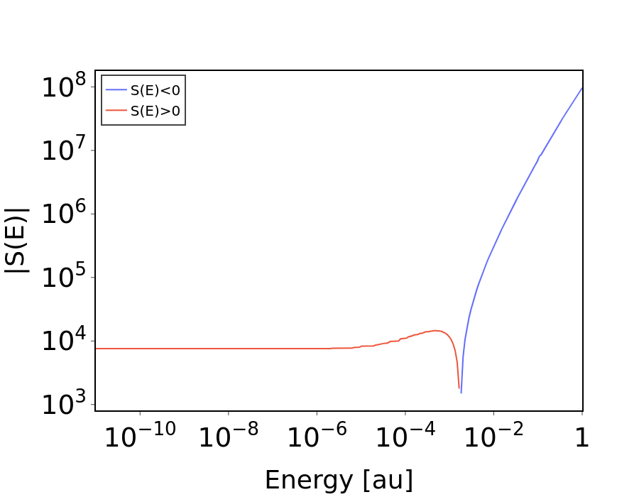
Figure 6: Behaviour of the function $|S(E)|$ with respect to the energy

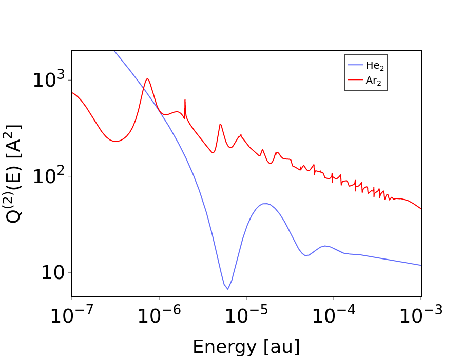
Figure 7: Comparison of the quantum collision cross-section $Q^{(2)}(E)$

of argon dimer (this work) and helium dimer (Ref.Czachorowski (2022)).

The calculations of $S(E)$ were carried out for $250$ values of the energy $E$, distributed logarithmically within the range from $10^{-11}$ to $1\,$a.u. For each energy, phase shifts were calculated as described in this section and in Ref. Wei and Le Roy (2006). The calculations were stopped when the relative contribution of a particular $l$ in Eq. 29 was smaller than $10^{-6}$% or $l<20\;000$. If a contribution for $l>20\;000$ was still significant, the Born approximation

$$\mathrm{tan}\delta_{l}=\frac{24\pi\mu_{a}C_{6}E^{2}}{(2l-3)(2l-1)(2l+1)(2l+3)(2l+5)},$$ (31)

was used to calculate the remaining contributions necessary to reach the threshold. In the above formula $\mu_{a}$ is the atomic mass, and $C_{6}$ is the total asymptotic coefficient, i.e., including the BO, relativistic and QED contributions. The calculated values of $S(E)$ are given in Fig. 6. The Born approximation was required for energies $E>10^{-3}$ a.u.  where the values of $S(E)$ are negative. For lower energies, angular momenta up to about $l=8\;000$ were sufficient.

The original set of $250$ energies is not large enough to properly describe the collision cross-sections, $Q^{(n)}(E)$. Therefore, we created an additional grid of $12\;000$ non-uniformly distributed points according to

$$E_{m}/\,\mathrm{K}=2\,(1.0005^{m}-1);\;\;m\in\{1,\cdots,12\;000\}.$$ (32)

As the contributions to $Q^{(n)}(E)$ decay much faster with increasing angular momentum than in the case of $S(E)$, the summations were truncated when the contribution from a given $l$ was smaller than $10^{-12}$ on a relative basis. On average, $l\approx 700$ was sufficient to reach this threshold, with an exception of higher energies for which $l\approx 1700$ is adequate. In Fig. 7, we present a comparison of the collision cross-sections $Q^{(2)}(E)$ for the argon dimer calculated in this work and for the helium dimer. Czachorowski et al. (2020); Czachorowski (2022)

VI Thermophysical properties

The second virial coefficient $B(T)$ can be expressed as a sum of three distinct parts

$$B(T)=B_{\mathrm{ideal}}(T)+B_{\mathrm{bound}}(T)+B_{\mathrm{thermal}}(T),$$ (33)

where $B_{\mathrm{ideal}}(T)$ is the contribution from the ideal gas formula, $B_{\mathrm{bound}}(T)$ is the contribution of the rovibrational states of the dimer, and $B_{\mathrm{thermal}}(T)$ is the atom-atom scattering contribution to the second virial coefficient. For the ⁴⁰Ar dimer, these contributions are defined as

$$B_{\mathrm{ideal}}(T)=-\frac{\Lambda(T)^{3}}{16},$$ (34)

$$B_{\mathrm{bound}}(T)=-\Lambda(T)^{3}\sum_{v,l}^{l\;\mathrm{even}}(2l+1)(e^{-E_{v,l}/k_{\mathrm{B}}T}-1),$$ (35)

$$B_{\mathrm{bound}}(T)=-\frac{\Lambda(T)^{3}}{\pi k_{\mathrm{B}}T}\int_{0}^{\infty}e^{-E/k_{\mathrm{B}}T}S(E)\;dE,$$ (36)

where $v$ and $l$ are the vibrational and rotational quantum numbers, respectively, of the bound states of the system, $E_{v,l}$ are energies of these bounds states, $S(E)$ is defined in Eq. (29), and $\Lambda(T)$ is

$$\Lambda(T)=\frac{h}{\sqrt{\pi 2\mu_{a}k_{\mathrm{B}}T}}.$$ (37)

The second acoustic coefficient $\beta(T)$ is defined using $B(T)$ and its first and second derivatives with respect to the temperature

$$\beta(T)=2B(T)+2(\gamma_{0}-1)T\frac{dB(T)}{dT}+\frac{(\gamma_{0}-1)^{2}}{\gamma_{0}}T^{2}\frac{d^{2}B(T)}{dT^{2}},$$ (38)

where $\gamma_{0}$ is the heat capacity ratio ($\gamma_{0}=5/3$ for a monatomic gas).

The transport coefficients can be obtained using the Chapman-Enskog method applied to the Boltzmann equation Chapman and Cowling (1970); Ferziger and Kaper (1973) with the help of the Sonine polynomial expansions as described in detail by Tipton et al. Loyalka et al. (2007); Tipton et al. (2009a, b). In this work, we consider two transport coefficients, namely the thermal conductivity, $\lambda$, and the viscosity, $\eta$. In the framework of Chapman and Enskog, the formula for the thermal conductivity is given by

$$\lambda(T)=\frac{75}{64}\frac{k_{\mathrm{B}}\sqrt{\pi 2\mu_{a}k_{\mathrm{B}}T}}{2\mu_{a}\Omega^{(2,2)(T)}}f_{\lambda}^{(m)}$$ (39)

and for the viscosity by

$$\eta(T)=\frac{5}{16}\frac{\sqrt{\pi 2\mu_{a}k_{\mathrm{B}}T}}{\Omega^{(2,2)(T)}}f_{\eta}^{(m)},$$ (40)

where $\Omega^{(n,s)}(T)$ is a collision integral depending on the quantum cross-section $Q^{(n)}(E)$, defined as follows

$$\begin{split}\Omega^{(n,s)}(T)&=\frac{(n+1)}{n(s+1)!(k_{\mathrm{B}}T)^{s+2}}\\ &\times\int_{0}^{\infty}Q^{(n)}(E)e^{-E/k_{\mathrm{B}}T}E^{s+1}\;dE,\end{split}$$ (41)

and $f_{\eta}^{(m)}$ and $f_{\lambda}^{(m)}$ are correction factors representing $m$-th order approximations of the kinetic theory Hirschfelder et al. (1964). In the first-order approximation we have $f_{\eta}^{(1)}=f_{\lambda}^{(1)}=1$ and higher-order approximations are close to this value. In general, $f_{\eta}^{(m)}$ and $f_{\lambda}^{(m)}$ depend on the collision integrals $\Omega^{(n,s)}(T)$; explicit expressions can be found in Ref. Viehland et al. (1995). For simplicity, we employ the fifth-order approximation in this work.

Formally, the integration limits in both Eq. (36) and Eq. (41) extend to infinity. In practice, a large but finite value of the upper integration limit is entirely sufficient, because the integrands in Eq.36 and Eq.41 vanish exponentially as a function of energy due to the Boltzmann factors. In our calculations, the upper limit of the integration was set to $1\,$a.u.

VI.1 Second pressure and acoustic virial coefficients

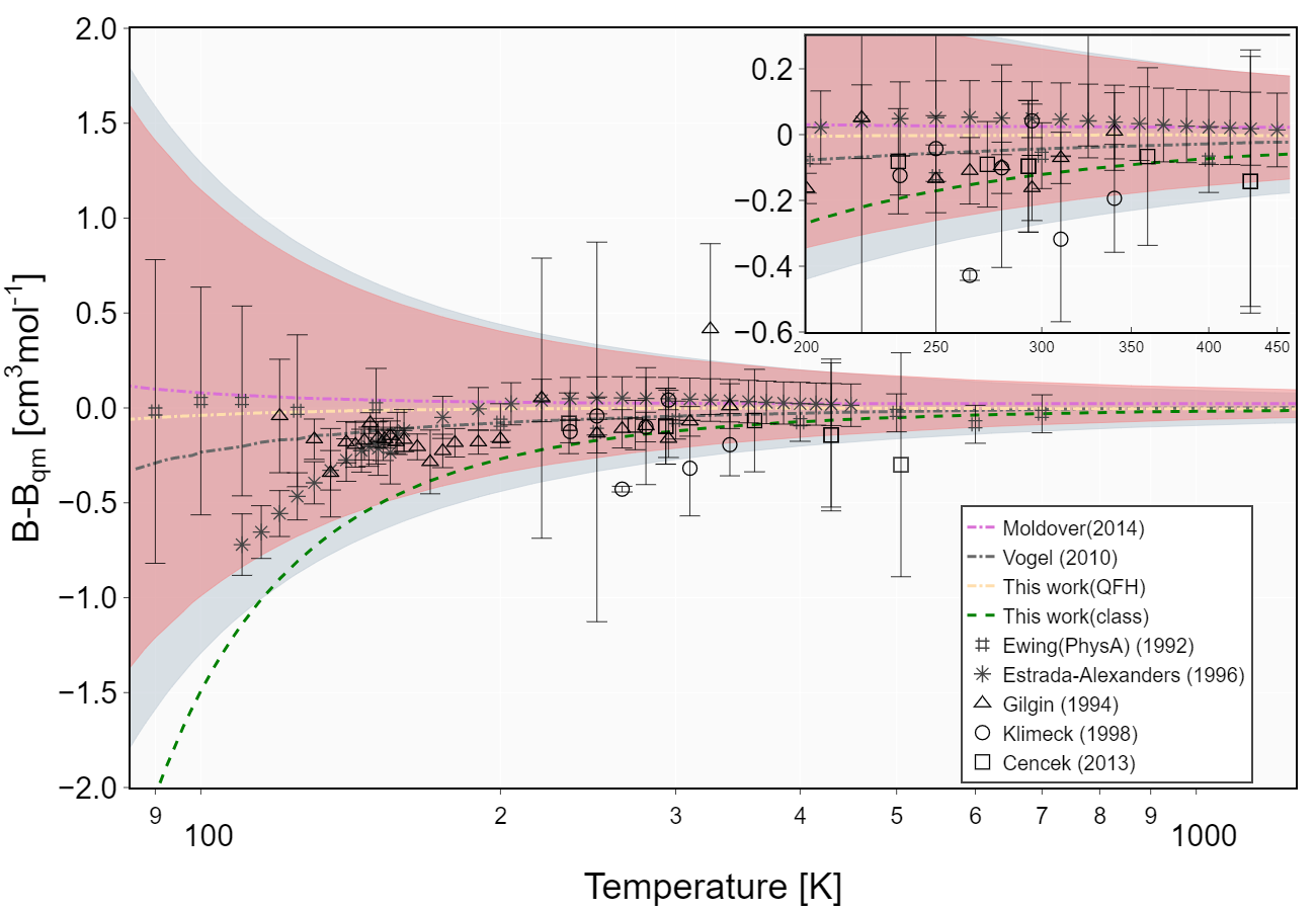
(a)

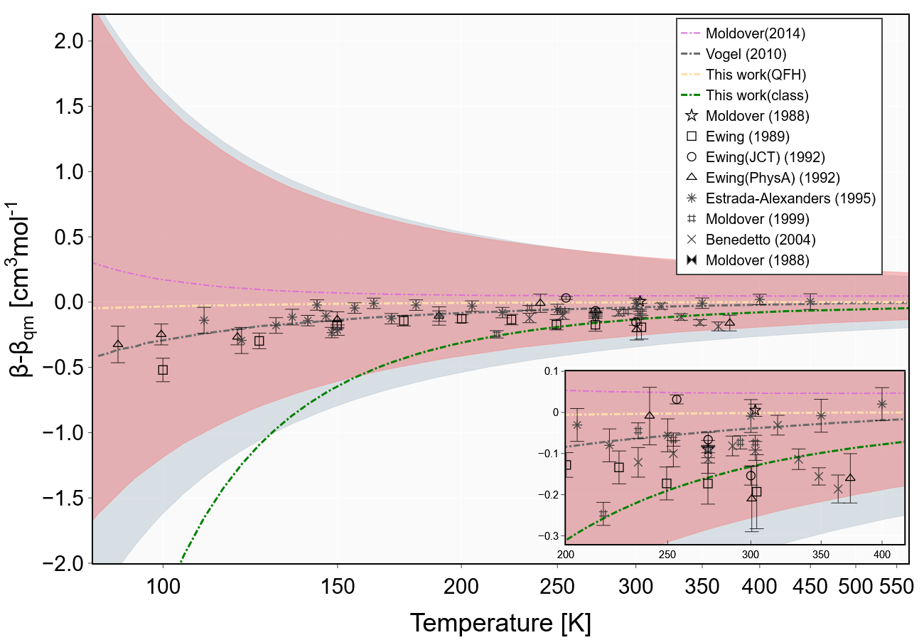
(b)

Figure 8: Deviations of the experimental and theoretical second pressure virial coefficients of Argon dimer from quantum mechanical values (a) $B_{\mathrm{qm}}(T)$ and (b) $\beta_{\mathrm{qm}}(T)$ calculated with the new interatomic potential. The dotted lines represent classical calculations and dash-dotted line corresponds to the semiclassical calculations. Semiclassical results of Moldover et al. were taken from supplement material of Ref. Moldover et al. (2014) and values obtained with potential of Jäger et al. from work of Vogel et al.Vogel et al. (2010). Red area corresponds to the uncertainty estimated in Ref. Moldover et al. (2014) for potential of and Szalewicztitet al. and gray area to uncertainty estimated for new potential in this work. Experimental results were obtained from Refs. Ewing and Goodwin (1992); Ewing and Trusler (1992); Estrada-Alexanders and Trusler (1996); Gilgen et al. (1994); Klimeck et al. (1998); Cencek et al. (2013); Moldover et al. (1999); Benedetto et al. (2004).

Recently, Myatt et al.Myatt et al. (2018) have consolidated and re-evaluated the available experimental results Ewing and Trusler (1992); Estrada-Alexanders and Trusler (1996); Sevast’yanov and Chernyavskaya (1987); Kestin et al. (1984); Michels et al. (1949); Gilgen et al. (1994); Klimeck et al. (1998); Cencek et al. (2013); Avdiaj and Delija (2022); Moldover and Trusler (1988); Ewing et al. (1989); Ewing and Goodwin (1992); Estrada-Alexanders and Trusler (1995); Moldover et al. (1999); Benedetto et al. (2004); May et al. (2007); Vogel (2010); Lin et al. (2014); Faubert and Springer (1972); Haarman (1973); Springer and Wingeier (1973); Chen and Saxena (1975); Fleeter et al. (1981); Clifford et al. (1981); Ziebland (1981); Kestin et al. (1982); Haran et al. (1983); Kestin et al. (1984); Johns et al. (1986); Mardolcar et al. (1986); Younglove and Hanley (1986); Millat et al. (1987); Hemminger (1987); Perkins et al. (1991); Roder et al. (2000); Sun and Venart (2005); May et al. (2007); Johnston and Grilly (1942); Flynn et al. (1963); Kestin and Nagashima (1964); Clarke and Smith (1968); Gracki et al. (1969); Dawe and Smith (1970); Kestin et al. (1972); Hellemans et al. (1974); Clifford et al. (1975); Vargaftik and Vasilevskaya (1984); Wilhelm and Vogel (2000); Evers et al. (2002); Vogel (2010); Berg and Moldover (2012); Berg and Burton (2013); Lin et al. (2014); Guevara et al. (1969) for several thermophysical properties of argon gas. In Figs. 8 we compare the experimental and theoretical second pressure and acoustic virial coefficients from our quantum mechanical calculations with the new argon dimer potential. As older experiments exhibit large uncertainties, we omit them and compare our results only with the newest experimental values Ewing and Trusler (1992); Estrada-Alexanders and Trusler (1996); Sevast’yanov and Chernyavskaya (1987); Kestin et al. (1984); Michels et al. (1949); Gilgen et al. (1994); Klimeck et al. (1998); Cencek et al. (2013); Avdiaj and Delija (2022); Moldover and Trusler (1988); Ewing et al. (1989); Ewing and Goodwin (1992); Estrada-Alexanders and Trusler (1995); Moldover et al. (1999); Benedetto et al. (2004). In the comparison in Figs. 8, we additionally include the semiclassical results of Moldover et al. Moldover et al. (2014) obtained using the potential of Ref. Patkowski and Szalewicz (2010) and results of Vogel et al. Vogel et al. (2010) based on potential of Ref. Jäger et al. (2009).

The virial coefficients calculated using all considered potentials agree with the exception of the potential from Ref. Sheng et al. (2020). While this potential produces accurate vibrational levels of argon dimer Sheng et al. (2020), it is not adequate for the calculations of the second pressure and acoustic virial coefficients. Indeed, the deviations of the second pressure and acoustic virial coefficients calculated with this potential from the newest experimental data range from 6% to 10% and from 4% to 10%, respectively. On the other hand, empirical potentials of Song et al. Song and Yang (2019), Deiters et al. Deiters and Sadus (2019), and Myatt et al. Myatt et al. (2018) exhibit much smaller differences and are well within the estimated uncertainties of this work for the most of the studied temperatures. The semiclassical results obtained using the refined potential are almost equal to the quantum mechanical results and suggest that the semiclassical calculations are sufficient for the accurate determination of the second pressure and acoustic virial coefficients of the argon. Indeed, the deviations between the quantum-mechanical and semiclassical calculations are $\leq 0.03\%$ for most of the studied temperature range (30 K-4000 K). This deviation increases slightly for smaller temperatures but even at 30 K, i.e., way below the freezing point of argon (83.95 K), the deviations are 0.03% and 0.16% for the second pressure and acoustic virial coefficients, respectively. We expect the same behavior for heavier noble gases such as krypton and xenon as their freezing points are much higher. The deviation of the second pressure and acoustic virial coefficients from the semiclassical results of Moldover et al.Moldover et al. (2014) and Vogel et al.Vogel et al. (2010) for selected temperatures are presented in Table 3. Not surprisingly, the results of Moldover et al. are close to ours as we share the same BO potential from Ref. Patkowski and Szalewicz (2010).

Table 3: Relative deviations $\Delta B_{\mathrm{scl}}=\frac{B_{\mathrm{qm}}-B_{\mathrm{scl}}}{B_{\mathrm{qm}}}$ and $\Delta\beta_{\mathrm{scl}}=\frac{\beta_{\mathrm{scl}}-\beta_{\mathrm{qm}}}{\beta_{\mathrm{qm}}}$ of semiclassical calculations of $B_{\mathrm{scl}}(T)$ and $\beta_{\mathrm{scl}}(T)$ using various potentials from the quantum mechanical calculations. Estimated uncertainties are presented in parentheses, units are $\mathrm{cm}^{3}\;\mathrm{mol}^{-1}$ and $\mathrm{cm}^{6}\;\mathrm{mol}^{-2}$ for second pressure virial and acoustic virial respectively.

	$B_{\mathrm{qm}}(T)$	$\Delta B_{\mathrm{scl}}(T)$			$RT\beta_{\mathrm{qm}}(T)$	$\Delta\beta_{\mathrm{scl}}(T)$
Temp.[K]	this work	Ref. Jäger et al. (2009)	Ref. Moldover et al. (2014)	this work	this work	Ref. Jäger et al. (2009)	Ref. Moldover et al. (2014)	this work
$90$	$-221.4(19)$	$0.13\%$	$-0.04\%$	$0.02\%$	$-229.0(20)$	$0.16\%$	$-0.11\%$	$0.02\%$
$110$	$-152.9(11)$	$0.13\%$	$-0.04\%$	$0.02\%$	$-144.7(13)$	$0.17\%$	$-0.09\%$	$0.02\%$
$200$	$-47.82(26)$	$0.16\%$	$-0.06\%$	$0.01\%$	$-23.85(53)$	$0.35\%$	$-0.22\%$	$0.02\%$
$280$	$-19.48(13)$	$0.25\%$	$-0.13\%$	$0.01\%$	$7.29(36)$	$-0.62\%$	$0.65\%$	$0.02\%$
$340$	$-8.223(95)$	$0.44\%$	$-0.28\%$	$0.01\%$	$19.40(30)$	$-0.15\%$	$0.24\%$	$<0.01\%$
$500$	$7.026(49)$	$-0.26\%$	$0.32\%$	$<0.01\%$	$35.24(21)$	$-0.02\%$	$0.13\%$	$<0.01\%$

Note that older experimental values of second virial coefficient follow the trend of the classical calculations. This behaviour is to be expected as most experiments determine the acoustic virial coefficients through the measurement of the speed of sound of the gas. The second virial coefficient is then evaluated from the second acoustic virial coefficient. As the derivatives of $B(T)$ with respect to the temperature are a priori unknown, they are often approximated from the classical or semiclassical calculations using the available dimer interaction potentials. Interestingly, the second acoustic virial coefficients obtained from the potential of Jäger et al. are almost identical to the experimental values. This is somewhat surprising as Jäger et al. Jäger et al. (2009) employed smaller basis sets in their calculation than and Szalewicztitet al. Patkowski and Szalewicz (2010) at the same level of theory. Nevertheless, the experimental values are within the calculated uncertainties of the quantum mechanical calculations and within the estimated uncertainties of Moldover et al. Moldover et al. (2014).

To best of our knowledge, in this work we report the first fully quantum-mechanical calculation of the second virial coefficients of the argon gas with rigorous error estimates. While Patkowski et al. provided uncertainty estimates for their potential at a set of grid of points, no systematic estimation of the uncertainties for the full potential was given. Therefore, it is unknown how Moldover et al. obtained their estimation of uncertainty, but they generally agree with our uncertainties obtained from calculations using the modified potentials, $V(R)\pm\sigma(R)$. The relative uncertainty of the second virial coefficients calculated by us is below $1.3\%$ for all temperatures, with the exception of a region where a change of sign occurs. This phenomena corresponds to about $408~{}K$ for the second pressure virial coefficient and $254~{}K$ for the second acoustic virial coefficient. The main source of uncertainty in our calculations comes from the BO contribution to the pair potential, as other sources of error, such as incomplete treatment of relativistic and QED effects, have been eliminated in the refined potential.

VI.2 Transport properties

A large number of experimental work on the viscosity and thermal conductivity was conducted on argon gas. This abundance is explained by relatively low cost of argon in comparison with other noble gases Faubert and Springer (1972); Haarman (1973); Springer and Wingeier (1973); Chen and Saxena (1975); Fleeter et al. (1981); Clifford et al. (1981); Ziebland (1981); Kestin et al. (1982); Haran et al. (1983); Kestin et al. (1984); Johns et al. (1986); Mardolcar et al. (1986); Younglove and Hanley (1986); Millat et al. (1987); Hemminger (1987); Perkins et al. (1991); Roder et al. (2000); Sun and Venart (2005); May et al. (2007); Johnston and Grilly (1942); Flynn et al. (1963); Kestin and Nagashima (1964); Clarke and Smith (1968); Gracki et al. (1969); Dawe and Smith (1970); Kestin et al. (1972); Hellemans et al. (1974); Clifford et al. (1975); Vargaftik and Vasilevskaya (1984); Wilhelm and Vogel (2000); Evers et al. (2002); Vogel (2010); Berg and Moldover (2012); Berg and Burton (2013); Lin et al. (2014); Guevara et al. (1969); Zhang et al. (2013); Xiao et al. (2020). Similarly to the virial coefficients, we consider only the experimental data that have been reported recently and have small uncertainties. Namely, we consider the results of Sun et al. Sun and Venart (2005), May et al. May et al. (2007), Vogel et al. Vogel (2010), Berg et al. Berg and Moldover (2012); Berg and Burton (2013), Lin et al. Lin et al. (2014), Zhang et al. Zhang et al. (2013), and Xiao et al. Xiao et al. (2020). In Fig. 9 we compare transport properties from the aforementioned experimental work and from theoretical quantum-mechanical calculations of Shapirov et al. Sharipov and Benites (2019) and semi-classical calculations of Vogel et al. Vogel et al. (2010), and Moldover et al. Moldover et al. (2014). Shapirov et al. used potential of Ref. Patkowski and Szalewicz (2010) and, to the best of our knowledge, provided the first fully quantum-mechanical results for the transport properties of various noble gases Sharipov and Benites (2019). Shapirov et al. also provided their estimations of uncertainty but only as a difference between values obtained from potentials of Ref. Patkowski and Szalewicz (2010) and Ref. Jäger et al. (2009). Surprisingly, the estimated uncertainty for temperatures below 300 K due was smaller ($10^{-4}$ or about 100 ppm) than the difference between semiclassical values of Vogel et al. and Moldover et al.. Our results for the viscosity are similar to the results of Shapirov for temperatures below 400 K, but differ by about 0.07% for higher temperatures. The difference between our values of the thermal conductivity and those of Sharipov is slightly larger but still within the estimated uncertainties of our calculations. Moldover et al. also provided uncertainty of their values, but the method of calculations of those uncertainties is unknown. Interestingly, our estimated uncertainties for both transport properties exhibit a minimum with values of $\approx$ 0.01% at around 400 K. Analogous minimum is also observed in the results of Moldover et al. (0.02%) at a similar temperature. In contrast to the second virial coefficients, the experimental uncertainties for the transport properties exceed the ab initio values reported in this work.

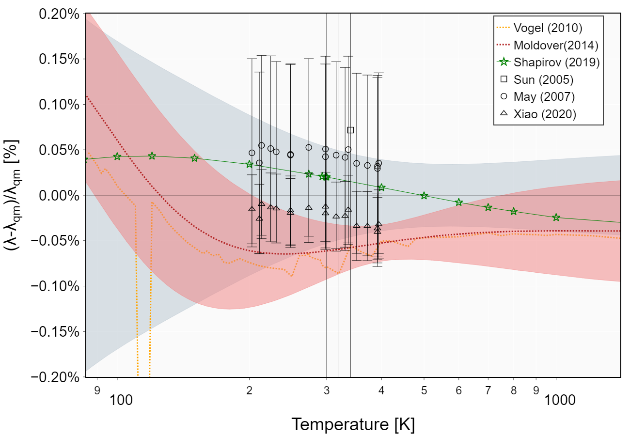
(a)

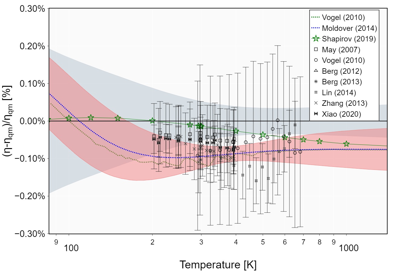
(b)

Figure 9: Relative deviations of the experimental and theoretical second pressure virial coefficients of Argon dimer from quantum mechanical values of (a) thermal conductivity $\lambda_{\mathrm{qm}}(T)$ and (b) viscosity $\eta_{\mathrm{qm}}(T)$ calculated with the new interatomic potential. Classical results of Moldover et al. were taken from supplement material of Ref. Moldover et al. (2014) and values obtained with potential of Jäger et al. from work of Vogel et al.Vogel et al. (2010). Red area corresponds to the uncertainty estimated in Ref. Moldover et al. (2014) for potential of titet al. and gray area to uncertainty estimated for new potential in this work. Experimental results were obtained from Refs. May et al. (2007); Vogel (2010); Lin et al. (2014); Zhang et al. (2013); Xiao et al. (2020)

VII Conclusions

In this work, we have developed a new ab initio interaction potential for the electronic ground state of the argon dimer. The Born-Oppenheimer component of the potential has been taken from Refs. Patkowski et al. (2005); Patkowski and Szalewicz (2010) and it cannot be improved with the computational resources available to us. However, we have refined the potential by including all sizeable post-Born-Oppenheimer effects. First, the relativistic corrections have been calculating using the full Breit-Pauli Hamiltonian, taking into account both one- and two-electron effects. Second, retardation of the electromagnetic interactions has been included in the long-range part of the potential and the leading-order quantum electrodynamics correction has been calculated.

Spectroscopic properties of the argon dimer such as vibrational energy levels, bond-dissociation energy, and rotational and centrifugal-distortion constants have been reported. Inclusion of the post-Born-Oppenheimer effects has resulted in destabilization of the previously discovered weakly bound ninth vibrational state. Thermophysical properties of the argon gas, namely pressure and acoustic virial coefficients, as well as transport properties – viscosity and thermal conductivity – have been determined using the newly developed potential. In the case of the thermophysical properties, the theoretical values reported here are somewhat less accurate than the most recent experimental data. However, the opposite is true for the transport properties – theoretical results calculated in this work have considerably smaller uncertainties than the data derived from measurements.