Shallow-Depth Variational Quantum Hypothesis Testing

Abstract

The task of discriminating between two known quantum channels is a well known binary hypothesis testing task. We present a variational quantum algorithm with a parameterized state preparation and two-outcome positive operator valued measure (POVM) which defines the acceptance criteria for the hypothesis test. Both the state preparation and measurement are simultaneously optimized using success probability of single-shot discrimination as an objective function which can be calculated using localized measurements. Under constrained signal mode photon number quantum illumination we match the performance of known optimal 2-mode probes by simulating a bosonic circuit. Our results show that variational algorithms can prepare optimal states for binary hypothesis testing with resource constraints.

Introduction.—

Quantum resources have been implied in the enhanced performance of technology tasks in the future such as computing, communication and hypothesis testing. In view of this, the presence of noisy intermediate scale quantum (NISQ) computers presents an opportunity to go beyond algorithms that are classical in nature Preskill (2018); Bharti et al. (2022). Variational quantum algorithms (VQAs) Cerezo et al. (2021a); McClean et al. (2016) and the quantum approximate optimization algorithm Farhi et al. (2014) are algorithms that solve optimization problems using quantum computers and are implementable for NISQ devices. VQAs are hybrid quantum-classical algorithms where the state preparation and measurement is simulated using a NISQ device implementing a parameterized quantum circuit (PQC) and parameter optimization is performed on a classical optimizer. VQAs have certain limitations such as barren plateaus in the optimization landscape due to both increased parameters McClean et al. (2018) and increased noise Wang et al. (2021) with large depth circuits. These can be avoided by designing VQAs which use local observables with low depth circuits Cerezo et al. (2021b) and certain transfer-learning inspired methods can mitigate barren plateaus as well Liu et al. (2023). Having said this, the potential applications of VQAs are numerous. VQAs have been employed to optimize ground state energies of molecular Hamiltonians Kandala et al. (2017); Peruzzo et al. (2014) with modified approaches to find energies for excited levels Jones et al. (2019). Optimal Ramsey interferometry Kaubruegger et al. (2021); Marciniak et al. (2022), estimation of quantum Fisher information Beckey et al. (2022) and distance measures between quantum states Chen et al. (2021) have also been implemented with the use of VQAs. Hence, shallow depth circuits with a demonstrable advantage are highly sought after.
In this manuscript, we propose a novel application of VQAs by demonstrating that shallow depth circuits can be employed for performing quantum channel discrimination. We apply our algorithm to the problem of quantum illumination Lloyd (2008); Shapiro and Lloyd (2009); Tan et al. (2008); Sanz et al. (2017); Fan and Zubairy (2018); Lee et al. (2021); Karsa et al. (2020), where we optimize the error probability as a function of the probe state and a suitably defined two-outcome measurement. We show that low-depth parameterized quantum circuits (PQCs) can obtain known optimal values for Chernoff bound and trace distance in the case of quantum illumination. We begin by establishing results for discrimination between quantum channels on $n$ qubits in the following section and extend our analysis numerically by simulating bosonic modes for quantum illumination.

Variational Quantum Hypothesis Testing.—

Our key insight is that shallow depth VQAs can perform binary hypothesis testing of two generic quantum channels. We assert that parameterized quantum circuits are able to recover known optima by providing analytical results for arbitrary quantum hypothesis testing tasks and numerical simulations for the task of Gaussian quantum illumination. We begin with a brief review of channel discrimination. Quantum channel discrimination aims at distinguishing two generic quantum channels $\mathcal{E}_{0}:L(\mathcal{H})\to L(\mathcal{H})$ and likewise $\mathcal{E}_{1}$ using measurements, with the set of linear operators defined as $L(\mathcal{H})$. Within the binary hypothesis framework, the null hypothesis $H_{0}$ corresponds to quantum channel $\mathcal{E}_{0}$ and the alternate hypothesis $H_{1}$ corresponds to $\mathcal{E}_{1}$. An input quantum state $\rho\in D(\mathcal{H}\otimes\mathcal{H})$ is sent to one of two channels creating the output states $\rho_{i}=(\mathcal{E}_{i}\otimes\mathbb{I})(\rho)$ ($i=0$ or $1$) Aharonov et al. (1998). Following this, a measurement is performed over these output states using the positive operator-valued measure (POVM) $\{\Gamma,\mathbb{I}-\Gamma\}$ where $\Gamma$ is a valid POVM element in $L(\mathcal{H}\otimes\mathcal{H})$. The measurement outcome corresponding to $\Gamma$ is the acceptance criteria for hypothesis $H_{0}$ and outcome $\mathbb{I}-\Gamma$ is the acceptance criteria for $H_{1}$. The type-I error (false positive) is defined as $\alpha=1-\text{Tr}(\Gamma\rho_{0})$ and type-II error (false negative) is defined as $\beta=\text{Tr}(\Gamma\rho_{1})$. Moving forward, we optimize the total error probability $(\alpha+\beta)/2$ under the assumption that either channel has equal likelihood to be applied.
In our protocol, one of the two channels is acted on the prepared state $\rho$ following which the outcome of the two element POVM $\{\Gamma,\mathbb{I}-\Gamma\}$ is used to determine the channel that had been applied. Optimal strategies differ based on whether the channel can be applied sequentially or in parallel Harrow et al. (2010); Bavaresco et al. (2021). In the parallel strategy Bavaresco et al. (2021), the channel is applied on $n$ copies of the initial state and the Holevo-Helstrom result bounds the total error probability for $\rho_{0}^{\otimes n}$ and $\rho_{1}^{\otimes n}$. This asymptotically decays exponentially with the exponent determined by the Chernoff bound between $\rho_{0}$ and $\rho_{1}$ Audenaert et al. (2007); Nussbaum and Szkoła (2009). In asymmetric hypothesis testing, only one of the types of errors is minimized while keeping the other one bounded. In either case of whether $\alpha$ is minimized while $\beta$ is bounded or if $\beta$ is minimized while $\alpha$ is bounded, the minimum error probability asymptotically decays as the quantum relative entropy between $\rho_{0}$ and $\rho_{1}$ following quantum Stein’s Lemma Li (2014); Hiai and Petz (1991); Ogawa and Nagaoka (2000). In the symmetric case, the minimum error probability for a single copy use of the map is $1/2-\|\mathcal{E}_{0}-\mathcal{E}_{1}\|_{\diamond}/4$ where $\|\mathcal{E}_{0}-\mathcal{E}_{1}\|_{\diamond}$ is the diamond distance between the two channels. This is defined as

$$\|\mathcal{E}_{0}-\mathcal{E}_{1}\|_{\diamond}=\sup_{\rho}(\|(\mathcal{E}_{0}\otimes\mathbb{I}_{\mathcal{H}})(\rho)-(\mathcal{E}_{0}\otimes\mathbb{I}_{\mathcal{H}})(\rho)\|_{1}),$$ (1)

where $\|A\|_{1}=\text{Tr}\sqrt{A^{\dagger}A}$ is the trace norm. This bound is a direct extension of the Holevo-Helstrom bound Holevo (1973); Helstrom (1969). The diamond distance provides a fundamental bound which holds true for all states in $D(\mathcal{H}\otimes\mathcal{H}^{\prime})$ with $\dim(\mathcal{H}^{\prime})\geq\dim(\mathcal{H})$ Aharonov et al. (1998) and hence optimizing over states in $D(\mathcal{H}\otimes\mathcal{H})$ is sufficient to reach an optimal probe.

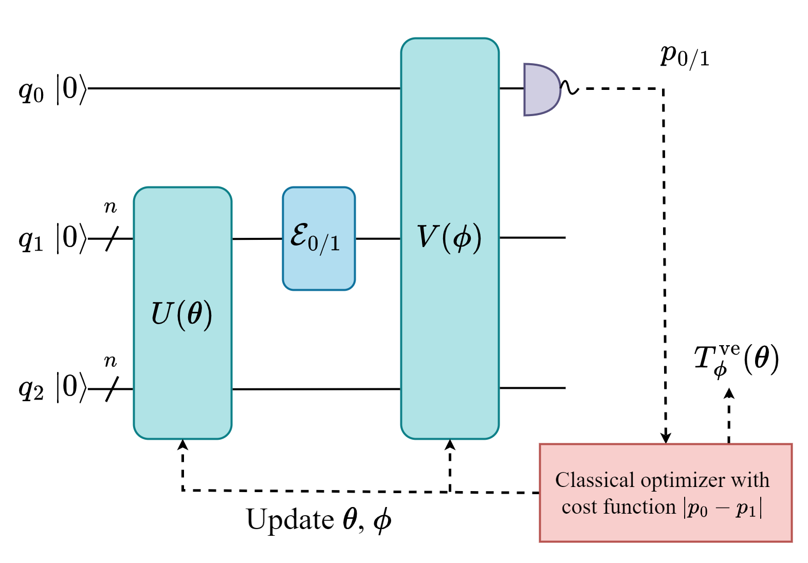
Figure 1: Circuit diagram for variational quantum hypothesis testing. The state preparation is over the two $n$ qubit registers $q_{1}$ and $q_{2}$. $q_{0}$ is used for measurements that are used to estimate the trace distance between the two states. The map is only applied over register $q_{1}$ and the optimization hence aims to prepare the state which gives the value of diamond distance as the trace distance between the states. For the case of quantum illumination considered below, $q_{i}$ represent bosonic modes as explained in the text.

For our variational algorithm, we prepare an entangled probe state $\rho_{\boldsymbol{\theta}}$ in registers $q_{1}$ and $q_{2}$ using the parameterized unitary $U(\boldsymbol{\theta})$ as depicted in Fig. 1. This is motivated by the advantage of entangled probe states D’Ariano et al. (2001); Bae et al. (2019); Piani and Watrous (2009); Aharonov et al. (1998) even in the case of entanglement breaking maps Sacchi (2005). Either the map $\mathcal{E}_{0}$ or $\mathcal{E}_{1}$ is then applied on the register $q_{1}$. The state after applying the map corresponding to the binary outcome $i=\{0,1\}$ is $\rho_{i,\boldsymbol{\theta}}=(\mathcal{E}_{i}\otimes\mathbb{I})(\rho_{\boldsymbol{\theta}})$.
The optimal protocol is achieved by maximizing the trace distance $\|\rho_{0,\boldsymbol{\theta}}-\rho_{1,\boldsymbol{\theta}}\|_{1}$, as is evident from (1). However, the direct evaluation of trace distance requires a tomographic reconstruction of the states being compared, which makes trace distance evaluation by tomographic and other methods difficult to use as a tool for variational hypothesis testing Chen et al. (2021); D’Ariano et al. (2003); Watrous (2008); Agarwal et al. (2021). We get around this by using an estimate of the trace distance as an objective function which makes use of a two-outcome POVM $\{\Gamma,\mathbb{I}-\Gamma\}$. The ancillary qubit $q_{0}$ (see Fig. 1) is used for measurements using the parameterized unitary $V(\boldsymbol{\phi})$ that encodes a Naimark extension Wilde (2013) of the POVM $\{\Gamma,\mathbb{I}-\Gamma\}$. The probability for outcome $\Gamma$ is $p_{i}=\text{Tr}(\Gamma\rho_{i,\boldsymbol{\theta}})=\text{Tr}\left((\outerproduct{0}{0}\otimes I)V(\boldsymbol{\phi})(\outerproduct{0}{0}\otimes\rho_{i,\boldsymbol{\theta}})V(\boldsymbol{\phi})^{\dagger}\right)$. Outcome $\Gamma$ is the acceptance criteria for hypothesis $H_{0}$ and $\mathbb{I}-\Gamma$ is the acceptance criteria for hypothesis $H_{1}$. Hence, $(p_{0}+1-p_{1})/2$ corresponds to the success probability in the classification task. We define a variational estimate of the trace distance $T^{\mathrm{ve}}_{\boldsymbol{\phi}}(\boldsymbol{\theta})$, which is always bounded above by the true trace distance and this bound is saturated when $V(\boldsymbol{\phi})$ encodes a Naimark extension of the Helstrom POVM Chen et al. (2021). The variational estimate of the trace distance is defined as

$$T^{\mathrm{ve}}_{\boldsymbol{\phi}}(\boldsymbol{\theta})=|p_{0}-p_{1}|\leq\frac{1}{2}\|\rho_{0,\boldsymbol{\theta}}-\rho_{1,\boldsymbol{\theta}}\|_{1}.$$ (2)

Our algorithm updates parameters to maximize $T^{\mathrm{ve}}_{\boldsymbol{\phi}}(\boldsymbol{\theta})$. $T^{\mathrm{ve}}_{\boldsymbol{\phi}}(\boldsymbol{\theta})$ is evaluated with a certain value of $\boldsymbol{\theta}$ and $\boldsymbol{\phi}$ using the quantum computer. These values are then fed into a classical optimizer which proposes updated parameter values for the next iteration and this is repeated till the convergence condition is met for the value of $T^{\mathrm{ve}}_{\boldsymbol{\phi}}(\boldsymbol{\theta})$. Once the convergence condition is met, the value of $\boldsymbol{\theta}$ and $\boldsymbol{\phi}$ are reported. The optimization aims to approach optimal values of $\boldsymbol{\theta}_{0},\boldsymbol{\phi}_{0}=\mathop{\mathrm{argmax}}_{\boldsymbol{\theta},\boldsymbol{\phi}}(T^{\mathrm{ve}}_{\boldsymbol{\phi}}(\boldsymbol{\theta}))$. Maximizing the value of $T^{\mathrm{ve}}_{\boldsymbol{\phi}}(\boldsymbol{\theta})$ clearly maximizes the success probability of discrimination.

While $T^{\mathrm{ve}}_{\boldsymbol{\theta}}(\boldsymbol{\phi})$ simplifies the optimization of trace distance by replacing true trace distance with $T^{\mathrm{ve}}$, the numerous parameters in the definitions of $U(\boldsymbol{\theta})$ and $V(\boldsymbol{\phi})$ may result in sub-optimal results. Suboptimality can arise in two ways, the first of which is that the optimization may fail to find the optimal states even if $U(\boldsymbol{\theta})$ is expressible enough for the optimal states. The second source of suboptimality could be that though the qubit measurements produce optimal states according to $T^{\mathrm{ve}}_{\boldsymbol{\theta}}(\boldsymbol{\phi})$, these optimized probe states might have a small trace distance evaluated by $T(\rho_{0,\boldsymbol{\theta}},\rho_{1,\boldsymbol{\theta}})$. The second source of suboptimality is different from the first since an expressible $U(\boldsymbol{\theta})$ is unrelated to the expressibility of $V(\boldsymbol{\phi})$, which is simultaneously required to ensure that the “good states are recognized”.
We now proceed to prove that if $U(\boldsymbol{\theta})$ and $V(\boldsymbol{\phi})$ are sufficiently expressible, the optimal states generated by the VQAs indeed optimize the real trace distance. This is to verify that our shallow depth circuits are sufficiently expressible for both state preparation and the measurements needed for hypothesis testing. To see this, consider a fixed $U(\boldsymbol{\theta})$ which generates a (perhaps) sub-optimal state and let us consider the optimization of $V(\boldsymbol{\phi})$. Since $V(\boldsymbol{\phi})$ represents the Naimark extension for an ideal two-outcome POVM, if $V(\boldsymbol{\phi})$ is expressible enough, then it is guaranteed that the optimization of $T^{\mathrm{ve}}_{\boldsymbol{\theta}}(\boldsymbol{\phi})$ converges to the real trace distance $T(\rho_{0,\boldsymbol{\theta}},\rho_{1,\boldsymbol{\theta}})$ (further discussed in appendix C). This argument was previously presented in Agarwal et al. (2021). Now, it is easy to see that if $U(\boldsymbol{\theta})$ is expressible, then the globally optimal states are expressible by the VQA. Judging the requirements on the expressibility of $U(\boldsymbol{\theta})$ can be done by considering the state preparation to occur using a control pulse $\gamma(t)$ which can be represented as $b_{\gamma}$ classical bits. We find that if the ideal probe state is reachable in polynomial time and we prepare $\rho_{\boldsymbol{\theta^{\prime}}}$ such that $\|\rho_{\boldsymbol{\theta}^{\prime}}-\rho_{\boldsymbol{\theta}_{0}}\|\leq\epsilon$, the true trace distance $T(\rho_{0,{\boldsymbol{\theta}^{\prime}}},\rho_{1,{\boldsymbol{\theta}^{\prime}}})\in[d(1-\epsilon),d]$ where $d=T(\rho_{0,{\boldsymbol{\theta}_{0}}},\rho_{1,{\boldsymbol{\theta}_{0}}})$ is the maximal trace distance. From the results in Lloyd and Montangero (2014) we know that $b_{\gamma}$ scales with $\log(1/\epsilon)$ and the dimension of the manifold of polynomial time reachable states and this gives us an estimate of how much information is needed for having a good state preparation. Further details on this can be found in appendix B. This completes the analysis that our VQAs can indeed theoretically find the optimal states and measurements to perform the hypothesis test. To prove that this theoretical result has practical applications in the real world, we apply our ideas to the example of Gaussian variational quantum illumination.

Gaussian variational quantum illumination.—

As a benchmark of our variational quantum hypothesis testing protocol, we study quantum illumination, which is an example with well-established analytical bounds. Quantum illumination Lloyd (2008); Shapiro and Lloyd (2009); Tan et al. (2008); Sanz et al. (2017); Fan and Zubairy (2018); Lee et al. (2021); Karsa et al. (2020) is the task of using entangled light to find out if a weakly reflective beam-splitter is present in a bright thermal bath. The exact form of the map acting on a 2-mode bosonic state $\rho_{SI}$ is given as $\mathcal{E}_{\eta}(\rho_{SI})=\text{Tr}_{S}(U_{\eta}(\rho_{B}\otimes\rho_{SI})U_{\eta}^{\dagger})$ where $U_{\eta}=\exp(i\sin^{-1}(\eta)(a_{S}^{\dagger}a_{B}-a_{S}a_{B}^{\dagger}))\otimes\mathbb{I}_{I}$ and $\rho_{B}$ is the thermal state with an average of $N_{B}$ photons. The hypothesis $H_{0}$ corresponds to the object being absent or equivalently beam-splitter has zero reflectivity hence is the map $\mathcal{E}_{\eta=0}$, and the hypothesis $H_{1}$ corresponds to the object being present with some weak reflectivity $r$ hence is the map $\mathcal{E}_{\eta=r}$. Despite clearly being an entanglement breaking map, there is an advantage in using a signal-idler entangled state as first demonstrated in Lloyd (2008). This advantage holds true even in the limit of $N_{B}\gg N_{S}$ where $N_{S}$ is the average number of signal photons Shapiro and Lloyd (2009); Tan et al. (2008).

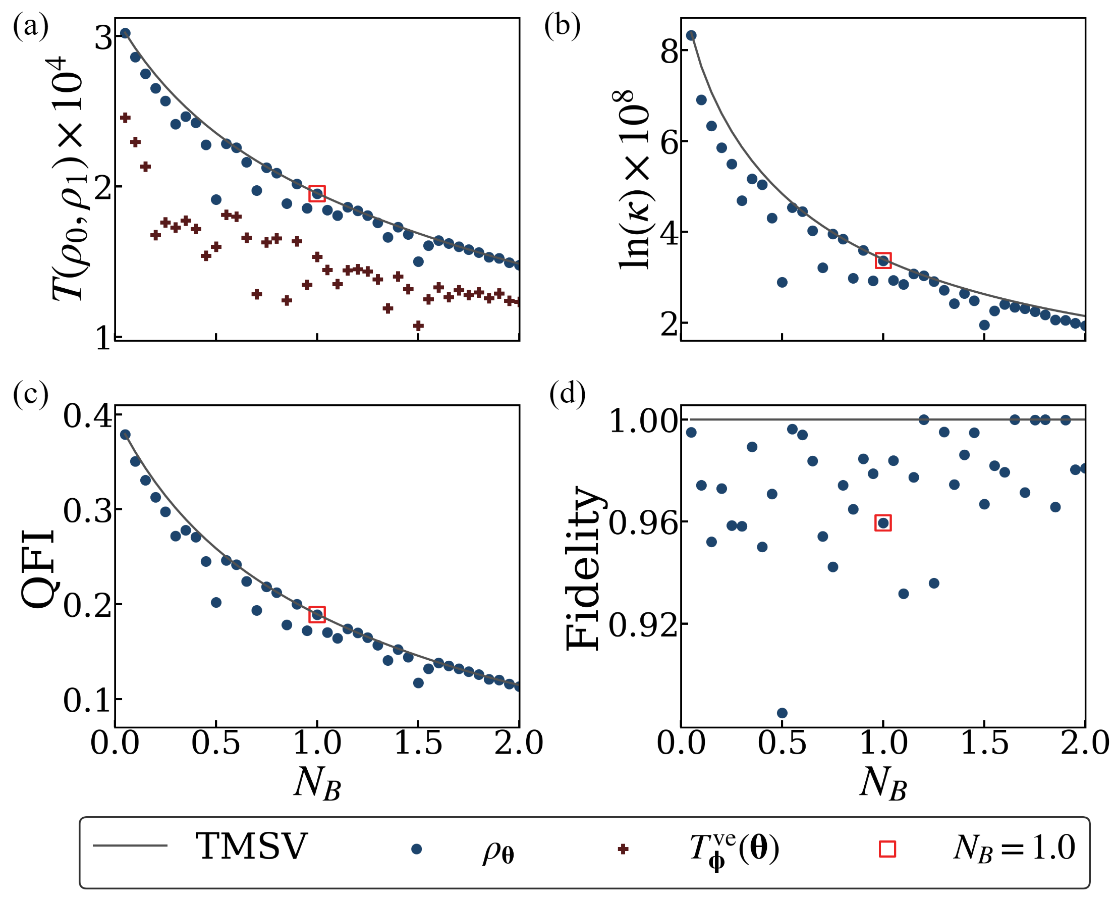
Figure 2: Simulation results with constrain $N_{S}=0.1$ using Gaussian backend of the Strawberry-fields package Bromley et al. (2020); Killoran et al. (2019). (a) Compares trace distance (blue dots are true trace distance and green triangles are estimated trace distance), (b) Compares Chernoff bound of the optimized state to TMSV, (c) compares QFI, and (d) shows fidelity of the optimized state to TMSV. The red square represents results optimized with $N_{B}=1.0$ and shows an optimized state with equivalent performance to the TMSV while not actually being equal to the TMSV.

The performance of a probe is judged by constraining the average photon number of the signal mode to be equal to $N_{S}$. This gives limits of the error probability to be related to the energy constrained diamond norm Winter (2017). All the results in this section are in the regime of a signal mode having a constrained photon number of $N_{S}$. Under this constraint, the optimal probe for the task of quantum illumination for single-shot discrimination is proven to be the two-mode squeezed vacuum state (TMSV) as shown in De Palma and Borregaard (2018); Bradshaw et al. (2021). The optimality of this state comes from the fact that it saturates the Chernoff bound Bradshaw et al. (2021) as well as the quantum relative entropy De Palma and Borregaard (2018) making it suitable for both symmetric and asymmetric hypothesis testing. Even when compared to non-Gaussian states such as a photon-added TMSV Noh et al. (2021), TMSV remains optimal for fixed $N_{S}$. We note that TMSV state is suboptimal for the Helstrom bound Bradshaw et al. (2021).
Our circuit for the task of variational quantum illumination follows the same protocol as that described in Fig. 1 except that now $q_{0}$ is a single bosonic mode, $q_{1}$ is a single bosonic mode labelled as the signal ($S$), and $q_{2}$ is a single bosonic mode labelled as the idler ($I$). We parameterize the unitary $U$ as coherent displacements followed by two mode squeezing each by variable parameters and the unitary $V$ as coherent displacements followed by conditional phase gates followed by beam-splitters. When given these resources and optimized, we note that our results match very closely to the optimal results of the TMSV (see Fig. 2). All unitary operations that take Gaussian states to Gaussian states can be broken down into the Bloch-Messiah decomposition Cariolaro and Pierobon (2016) which represents such unitaries as a passive operation followed by single mode squeezing on all modes followed by another passive operation where each passive operation is a photon number conserving operation which can be represented using beam-splitters and phase operations. While this is sufficient for complete parameterization for $n$-mode Gaussian states, we opt for a hardware-efficient ansatz Kandala et al. (2017) to see the performance of the algorithm in the restricted setting of having $U$ and $V$ both be composed of single mode operations such as displacements followed by limited two-mode operations such as beam-splitters.
The unitary $V$ encodes the Naimark extension of a two outcome POVM by having the vacuum state measurement on mode $q_{0}$ correspond to applying a joint POVM on the signal-idler state. One can always construct a unitary transformation acting on $q_{0}\otimes q_{1}\otimes q_{2}$ to transform a projective measurement on $q_{0}$ to a projective measurement in the space of $q_{1}\otimes q_{2}$ Buscemi et al. (2005). The procedure to construct unitary transformations using purely Gaussian operations is summarized in the appendix D.

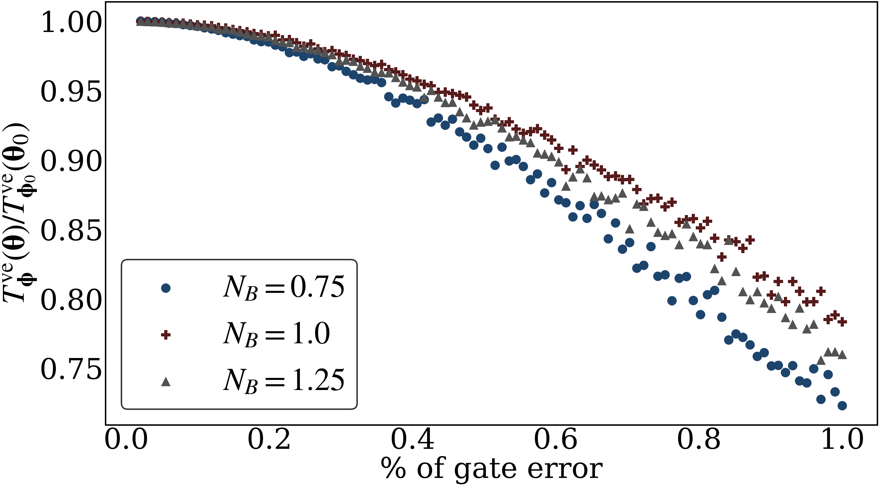
Figure 3: Noise robustness of variational quantum illumination. The quantity on $y$ axis is the ratio of $T^{\mathrm{ve}}_{\boldsymbol{\phi}}(\boldsymbol{\theta})$ to the value it takes with zero gate error. These are results that have been optimized with the constraint that $N_{S}=0.1$ following which the optimized results were then simulated with Gaussian noise for each parameter to test robustness. The values plotted are the average after 500 runs with the Gaussian noise with percentage of gate error being the variance.

To analyze these results, we note that the optimization goal is maximizing $T^{\mathrm{ve}}_{\boldsymbol{\theta}}(\boldsymbol{\phi})$. In Fig. 2(a) we highlight both the actual trace distance (blue dots) and the estimated trace distance (brown + symbols) after optimization. As can be seen by the value of the true trace distance, the optimization regularly is able to find the true optimum, in this case given by the TMSV state. Fig. 2(b) shows that the optimality of TMSV for Chernoff bound is nearly matched with our low depth circuit that optimizes $T^{\mathrm{ve}}_{\boldsymbol{\theta}}(\boldsymbol{\phi})$. This shows that despite optimizing for single-copy discrimination, it is able to optimize to the state which is asymptotically optimal for $n$ copies. Given that the family of maps $U_{\eta}$ is continuous, we see that our technique can be considered as a quantum sensing task, as noted in Tsang (2012). In the limit of $N_{S}\to 0$, the optimal quantum Fisher information (QFI) for this sensing task is given by the TMSV Sanz et al. (2017). In Fig. 2(c) we compare the QFI of the optimized state to this optimal value and observe that it demonstrates capability as a good sensing probe despite being trained for only a fixed value of $\eta$. Fig. 2(d) shows that despite reaching near the performance of the TMSV, the optimized states are not exactly equal to the TMSV, implying the existence of a manifold of states that perform just as well as the TMSV. We consider an example with $N_{B}=1.0$ (red square) which matches the performance of the TMSV constrained with $N_{s}=N_{I}=0.1$, yet it actually has average photons in idler and signal as $N_{I}\approx 0.17$ and $N_{S}=0.1$ showing clearly its difference from the ideal TMSV state. Furthermore, the reduced entropy and the coefficients of the Schmidt decomposition are different (see appendix E for details), demonstrating that the are not equivalent upto local one mode unitary transformations.

Discussion.—

Hypothesis testing is a task central to probability theory for the discrimination of probability distributions Scott and Nowak (2005). Quantum hypothesis testing extends this to quantum channel discrimination and quantum state discrimination. The use of quantum resources have demonstrated an advantage here and have applications in exoplanet spectroscopy Huang et al. (2023), superresolution between two incoherent optical sources Tsang et al. (2016), and as discussed in this work, quantum illumination Lloyd (2008); Shapiro and Lloyd (2009); Tan et al. (2008); Sanz et al. (2017); Fan and Zubairy (2018); Lee et al. (2021); Karsa et al. (2020).
In this work we have demonstrated how VQAs can be applied for the task of quantum hypothesis testing by analyzing the particular case of channel discrimination. By applying our VQA for the task of quantum illumination, we find that our optimization protocol is able to find a probe state which matches the optimal performance under signal photon number constraint as shown in Fig. 2. Additionally, as demonstrated in Fig. 3, these optimized results scale favorably with gate errors which shows noise resilience of the protocol. This supports the experimental viability of such algorithms for near-term quantum devices Preskill (2018); Bharti et al. (2022).
Our general results on quantum hypothesis testing have direct application in general channel discrimination Chiribella et al. (2008a, a) and tasks such as quantum reading Pirandola (2011); Ortolano et al. (2021). It must be noted that the related generalized tasks such as the testing of a quantum channel to be an isometry, the determination of distinguishability between $k$ input states for a quantum channel, or checking equality of two unitaries are QMA-complete Rosgen (2011); Beigi and Shor (2008); Janzing et al. (2005). We find that the information content of a control pulse required to make the trace distance between the states lie in $[d(1-\epsilon),d]$ (where $d$ is the maximum possible trace distance between the states obtained on sending a probe state through the channels) scales as $\log(1/\epsilon)$ if the optimal state itself is polynomially reachable. Hence our algorithm would also take exponential resources to converge for difficult tasks, which situates general complexity-theoretic results within our framework.
Having noted this, we further note that our algorithm performs well as benchmarked by channel discrimination measures. The algorithm achieves very close to optimal results for the discrimination between 2-qubit unitaries (see details in appendix A). While in this manuscript, we discuss the case of applying the channel only once on a single copy of the state, this can be clearly generalized to sequential and parallel channel discrimination Bavaresco et al. (2021). Such sequential and parallel channel discrimination have practical applications in a variety of tasks such as quantum metrology and certifying quantum circuits Chiribella et al. (2008b). Furthermore we speculate that via the Pinsker’s inequality Hirota (2020) which lower bounds quantum relative entropy in terms of the trace distance, we can generalize our algorithm to asymmetric QHT Spedalieri and Braunstein (2014). Hence variational quantum hypothesis testing is sure to find disparate applications in future quantum technologies.

Appendix: Shallow-Depth Variational Quantum Hypothesis Testing

Appendix A Appendix A: Diamond norm estimation

We have two quantum channels $\mathcal{E}_{0}:L(\mathcal{H})\to L(\mathcal{H})$ and $\mathcal{E}_{1}:L(\mathcal{H})\to L(\mathcal{H})$ where $L(\mathcal{H})$ is the set of linear operators from Hilbert space $\mathcal{H}$ to $\mathcal{H}$. We denote subset of $L(\mathcal{H})$ that are density operators as $D(\mathcal{H})$. We proceed on the task of channel discrimination, and as highlighted in the main text, we pick a state $\rho\in D(\mathcal{H}\otimes\mathcal{H})$ as a probe to the map $\mathcal{E}_{i}\otimes\mathbb{I}_{\mathcal{H}}$ ($i=0$ or $1$) and then use a POVM $\{\Gamma,\mathbb{I}-\Gamma\}$ for classification. We present this as an algorithm for estimation of diamond distance as well.
Using the parameterized circuit shown in Fig. 1 of the letter, we define the state after applying the map as $\rho_{i,\boldsymbol{\theta}}=(\mathcal{E}_{i}\otimes\mathbb{I})(\rho_{\boldsymbol{\theta}})$ and $p_{i}=\text{Tr}(\Gamma\rho_{i,\boldsymbol{\theta}})$. If the unitary $V(\boldsymbol{\phi})$ encodes the Naimark extension of the POVM $\{\Gamma,\mathbb{I}-\Gamma\}$, we obtain $p_{i}=\text{Tr}\left((\outerproduct{0}{0}\otimes I)V(\boldsymbol{\phi})(\outerproduct{0}{0}\otimes\rho_{i,\boldsymbol{\theta}})V(\boldsymbol{\phi})^{\dagger}\right)$. From this we define the cost function in the following equation which is bounded above by the diamond distance since the diamond distance is defined as the supremum of $\|\rho_{0,\boldsymbol{\theta}}-\rho_{1,\boldsymbol{\theta}}\|_{1}$ over all possible $\rho\in D(\mathcal{H}\otimes\mathcal{H})$.

$$T^{\mathrm{ve}}_{\boldsymbol{\phi}}(\boldsymbol{\theta})=|p_{0}-p_{1}|\leq\frac{1}{2}\|\rho_{0,\boldsymbol{\theta}}-\rho_{1,\boldsymbol{\theta}}\|_{1}\leq\frac{1}{2}\|\mathcal{E}_{0}-\mathcal{E}_{1}\|_{\diamond}$$ (3)

Take input as $\mathcal{E}_{0}$ and $\mathcal{E}_{1}$ which are CPTP maps from density matrices in $\mathcal{H}$ to density matrices in $\mathcal{H}$.

Initialize $\boldsymbol{\theta}$ and $\boldsymbol{\phi}$ which are parameters for $U(\boldsymbol{\theta})$ and $V(\boldsymbol{\phi})$.

Define convergence condition for cost function $T^{\mathrm{ve}}_{\boldsymbol{\phi}}(\boldsymbol{\theta})$.

while $T^{\mathrm{ve}}_{\boldsymbol{\phi}}(\boldsymbol{\theta})$ has not converged do

       for $\boldsymbol{\theta}_{i}=\boldsymbol{\theta}+\Delta\boldsymbol{\theta}_{i}$ and $\boldsymbol{\phi}_{i}=\boldsymbol{\phi}+\Delta\boldsymbol{\phi}_{i}$ for some set of $\Delta\boldsymbol{\theta}_{i}$ and $\Delta\boldsymbol{\phi}_{i}$ do

             Run circuit with parameters $\boldsymbol{\theta}_{i}$ and $\boldsymbol{\phi}_{i}$ with CPTP map as $\mathcal{E}_{0}\otimes\mathbb{I}_{n}$

             Using measurements on $q_{0}$ obtain value of $p_{0}$.

             Run circuit with parameters $\boldsymbol{\theta}_{i}$ and $\boldsymbol{\phi}_{i}$ with CPTP map as $\mathcal{E}_{1}\otimes\mathbb{I}_{n}$

             Using measurements on $q_{0}$ obtain value of $p_{1}$.

             Assign $T^{\mathrm{ve}}_{\boldsymbol{\phi}_{i}}(\boldsymbol{\theta}_{i})=|p_{0}-p_{1}|$

       end for

      Using $T^{\mathrm{ve}}_{\boldsymbol{\phi}_{i}}(\boldsymbol{\theta}_{i})$ update $\boldsymbol{\theta}$ and $\boldsymbol{\phi}$ with a classical optimizer.

       Check convergence of $T^{\mathrm{ve}}_{\boldsymbol{\phi}}(\boldsymbol{\theta})$.

end while

Assign estimated diamond norm $=2T^{\mathrm{ve}}_{\boldsymbol{\phi}}(\boldsymbol{\theta})$

return final values of $\boldsymbol{\theta}$, $\boldsymbol{\phi}$ and estimated diamond norm.

Algorithm 1 Variational quantum algorithm to estimate diamond distance

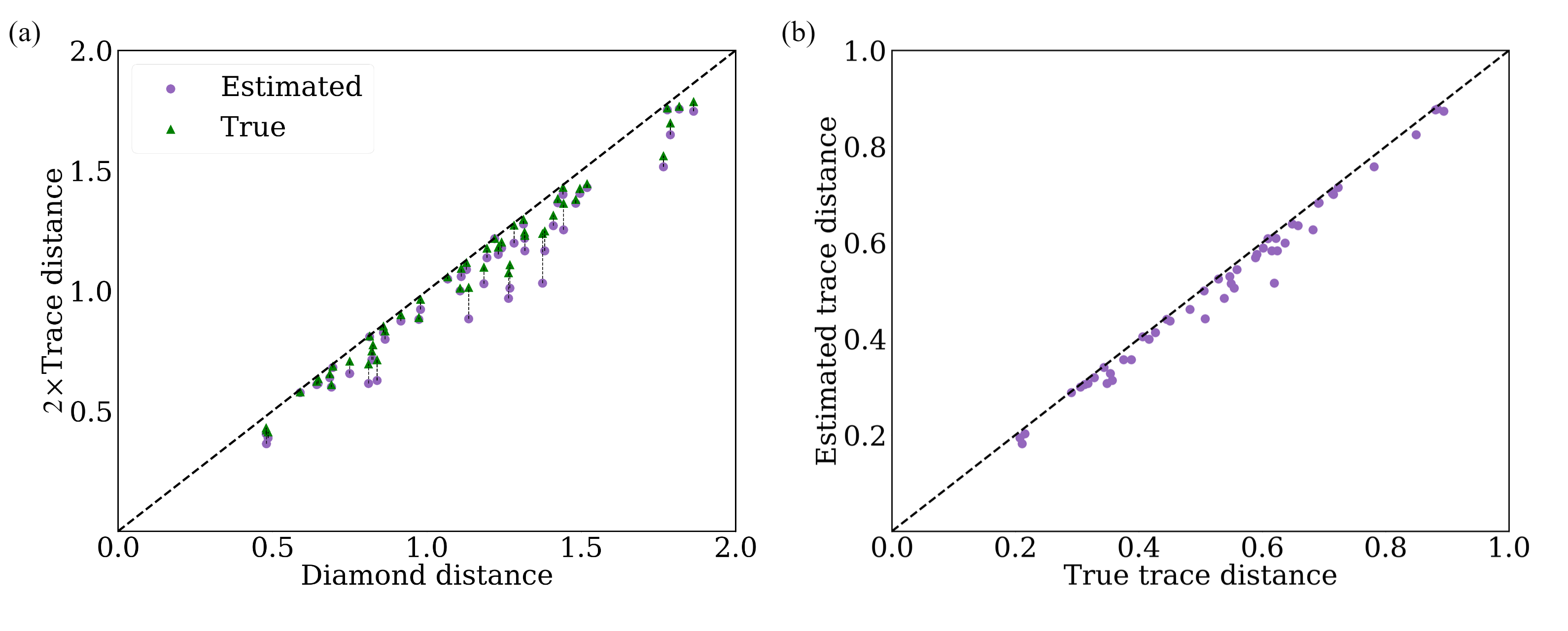
Figure 4: Estimation for diamond distance between the identity map and an arbitrary $2$ qubit unitary map. In these examples, the diamond distance between two randomly sampled 2-qubit unitaries is studied using the QHT algorithm we propose. (a) Shows how well the value of estimated $T^{\mathrm{ve}}_{\boldsymbol{\phi}}(\boldsymbol{\theta})$ and the true trace distance $T(\mathcal{E}_{0}(\rho_{\boldsymbol{\theta}}),\mathcal{E}_{1}(\rho_{\boldsymbol{\theta}}))$ for the optimized state matches against the analytical value. (b) Shows how well the estimated trace distance matches against the true trace distance for the state $\rho_{\boldsymbol{\theta}}$

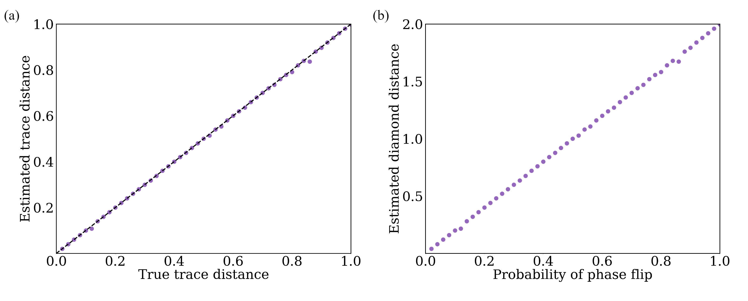
Figure 5: Estimation for diamond distance between the identity map and a phase flip map. In these examples the diamond distance between phase flip maps of form $\mathcal{E}(\rho)=(1-p)\rho+pZ\rho Z$ on 2-qubits is studied using our QHT algorithm. (a) Shows how well the estimated trace distance matches against the true trace distance for the state $\rho_{\boldsymbol{\theta}}$. (b) Shows the result of the estimated diamond norm against the probability of phase flip.

There are existing ways to find the diamond distance in $\mathcal{O}(poly(\dim{\mathcal{H}}))$ since it is a convex optimization problem Ben-Aroya and Ta-Shma (2009) but this clearly will grow exponentially in size as we increase the number of qubits. Our algorithm is clearly scalable for such situations and can produce results using a hardware efficient ansatz.
Figures 4 and 5 show results of simulations for estimating of diamond norm. The diamond distance between a unitary map and the identity map is the diameter of the circle which is able to contain all the eigenvalues of the unitary operation Benenti and Strini (2010). For Kraus maps such as the phase flip map of form $\mathcal{E}(\rho)=(1-p)\rho+pZ\rho Z$ have a diamond distance of $2p$ from the identity map Watrous (2008).
The simulations were carried out using QuTip Johansson et al. (2012, 2013). The circuit had five qubits with one of them being used in the trace distance estimation subroutine and the other four being used for state preparation after which the quantum map is applied on the first two of the four. The ansatz used was a hardware efficient ansatz Kandala et al. (2017) where we have single qubit rotations followed by an entangling operation which in this case is made of only CZ gates.

Appendix B Appendix B: Information content for optimal hypothesis testing

In this section we analyze the minimum amount of information content required for reaching an $\epsilon$-neighbourhood of the state which is optimal for hypothesis testing. This is to understand how much expressibility the ansatz used for state preparation requires to get a sufficiently good probe state. Here we consider the quantum channels $\mathcal{E}_{0}:L(\mathcal{H})\to L(\mathcal{H})$ and $\mathcal{E}_{1}:L(\mathcal{H})\to L(\mathcal{H})$ which satisfy the relation $\|((\mathcal{E}_{0}-\mathcal{E}_{1})\otimes\mathbb{I})\rho_{\mathrm{ideal}}\|_{1}=\|\mathcal{E}_{0}-\mathcal{E}_{1}\|_{\diamond}=d$.
To be able to reach the state $\rho_{\mathrm{ideal}}$ requires providing some classical information which encodes the quantum control problem of approaching this state. We assume that $\rho_{\mathrm{ideal}}\in\mathcal{W}^{+}$ which is the set of time-polynomial reachable states in $D(\mathcal{H}\otimes\mathcal{H})$ using a certain control scheme $\gamma(t)$ where the set of reachable states are $\mathcal{W}$. Let there be a state $\rho_{\mathrm{real}}$ in the epsilon neighbourhood of $\rho_{\mathrm{ideal}}$

$$\|\rho_{\mathrm{ideal}}-\rho_{\mathrm{real}}\|_{1}\leq\epsilon.$$ (4)

Using the results of Lloyd and Montangero (2014), the number of bits which can encode the control pulse $\gamma(t)$ must satisfy

$$b_{\gamma}\geq\dim(\mathcal{W}^{+})\log_{2}\left(\frac{1}{\epsilon}\right)$$ (5)

This can be understood by dividing the space of $\mathcal{W}^{+}$ into epsilon balls which would have a volume scaled as $\varepsilon^{\dim(\mathcal{W}^{+})}$ with respect to the total volume of the space. The information content in $\gamma(t)$ must be enough to specify the epsilon ball which we wish to be in which leads directly to (5). We define the operator $T=(\mathcal{E}_{1}-\mathcal{E}_{0})\otimes\mathbb{I}$ and the operator norm $\|T\|_{1}=\sup_{\rho}\|T\rho\|$ for $\rho\in D(\mathcal{H}\otimes\mathcal{H})$. We can take note of the following from the properties of the diamond norm Aharonov et al. (1998).

$$\|T\rho_{\mathrm{real}}\|_{1}\leq\|T\rho_{\mathrm{ideal}}\|=d$$ (6)

$$\|T(\rho_{\mathrm{ideal}}-\rho_{\mathrm{real}})\|_{1}\leq\|T\|_{1}\|(\rho_{\mathrm{ideal}}-\rho_{\mathrm{real}})\|_{1}\leq d\varepsilon$$ (7)

Using the triangle inequality for the 1-norm we obtain

$$\|T(\rho_{\mathrm{ideal}}-\rho_{\mathrm{real}})\|_{1}\geq\left|\|T\rho_{\mathrm{ideal}}\|_{1}-\|T\rho_{\mathrm{real}}\|_{1}\right|=d-\|T\rho_{\mathrm{real}}\|_{1}\geq 0$$ (8)

Combining the above inequalities, we obtain

$$0\leq d-\|T\rho_{\mathrm{real}}\|_{1}\leq d\epsilon\implies\|T\rho_{\mathrm{real}}\|_{1}\in[d(1-\varepsilon),d]$$ (9)

Notably the minimal $b_{\gamma}$ is independent of $d$. This expression shows that being in the $\varepsilon$ neighbourhood of the state which maximizes trace distance implies that the trace distance now lies between $d(1-\varepsilon)$ and $d$ irrespective of the value of $d$ and will require the same amount of classical information. The computational toughness will arise in the fact that if $d$ is small enough, even the best possible state is unable to tell apart the two channels.

Appendix C Appendix C: Simultaneous optimization in the algorithm

In this section we will prove that the method of simultaneous optimization employed for the algorithm used for variational quantum hypothesis testing is valid. We first begin with defining the form of our estimated trace distance. There are ways of estimating trace distance using a variational quantum algorithm as shown in Chen et al. (2021) and Agarwal et al. (2021). The main clue lies in the following definition of trace distance.

$$T(\rho_{0},\rho_{1})=\sup_{P\leq\mathbb{I}}(\text{Tr}(P(\rho_{0}-\rho_{1})))$$ (10)

We can variationally optimize the POVM $P$ to obtain an estimate of the trace distance. To do this using a unitary operation, we must embed the POVM into the unitary operator. For this the Naimark extension can be used Wilde (2013).

Theorem C.1 (Naimark extension).

For any POVM $\{\Gamma_{i}\}_{i\in O}$ acting on a system $S$, there exists a unitary $U_{PS}$ (acting on a probe system $P$ and the system $S$) and an orthonormal basis $\{\ket{i}_{P}\}_{i\in O}$ such that

$$\text{Tr}\left((\outerproduct{i}{i}\otimes I_{S})U_{PS}(\outerproduct{i}{i}\otimes\rho_{S})U_{PS}^{\dagger}\right)=\text{Tr}(\Gamma_{i}\rho_{S})$$ (11)

As pointed out in Wilde (2013), the two-outcome POVM $\{\Gamma,\mathbb{I}-\Gamma\}$ can be encoded in the following unitary with the probe system being a qubit.

$$U_{PS}=\mathbb{I}_{P}\otimes(\sqrt{\Gamma})_{S}+i(\sigma_{Y})_{P}\otimes(\sqrt{\mathbb{I}-\Gamma})_{S}$$ (12)

Let us define a parameterized unitary $V(\phi)$ which acts over both the probe and the system. We define the following quantity as an estimate of trace distance,

$$T_{\boldsymbol{\phi}}(\rho_{0},\rho_{1})=|p_{0}-p_{1}|$$ (13)

$$p_{i}=\text{Tr}\left((\outerproduct{0}{0}\otimes I)V(\boldsymbol{\phi})(\outerproduct{0}{0}\otimes\rho_{i})V(\boldsymbol{\phi})^{\dagger}\right)\quad i\in\{0,1\}$$ (14)

On combining theorem 4.1 and equation (10), we get that $\forall{\boldsymbol{\phi}}(T_{\boldsymbol{\phi}}(\rho_{0},\rho_{1})\leq T(\rho_{0},\rho_{1}))$. This is the main crux of using a variational algorithm for estimating trace distance in Chen et al. (2021). As an extension to this, we define the following cost function for our algorithm where we use an additional qubit as the probe subsystem.

$$T^{\mathrm{ve}}_{\boldsymbol{\phi}}(\boldsymbol{\theta})=|p_{0}(\boldsymbol{\theta},\boldsymbol{\phi})-p_{1}(\boldsymbol{\theta},\boldsymbol{\phi})|$$ (15)

$$p_{i}(\boldsymbol{\theta},\boldsymbol{\phi})=\text{Tr}\left((\outerproduct{0}{0}\otimes I)V(\boldsymbol{\phi})(\outerproduct{0}{0}\otimes\mathcal{E}_{i}(\rho(\boldsymbol{\theta})))V(\boldsymbol{\phi})^{\dagger}\right)\quad i\in\{0,1\}$$ (16)

Our optimization procedure will have to optimize both $\boldsymbol{\theta}$ and $\boldsymbol{\phi}$ for obtaining the best possible state preparation and measurement. Let us define $\boldsymbol{\theta}_{0}$ and $\boldsymbol{\phi}_{0}$ as follows

$$\boldsymbol{\theta}_{0} =\mathop{\mathrm{argmax}}_{\boldsymbol{\theta}}(\|\mathcal{E}_{1}(\rho_{\boldsymbol{\theta}})-\mathcal{E}_{0}(\rho_{\boldsymbol{\theta}})\|_{1})$$ (17)

$$\boldsymbol{\phi}_{0} =\mathop{\mathrm{argmax}}_{\boldsymbol{\phi}}(T^{\mathrm{ve}}_{\boldsymbol{\phi}}(\boldsymbol{\theta}_{0}))$$ (18)

Here $\boldsymbol{\theta}_{0}$ optimizes toward the state that saturates the Holevo-Helstrom bound Holevo (1973); Helstrom (1969). As per the definition of the optimization problem of trace distance estimation Chen et al. (2021), $\boldsymbol{\phi}_{0}$ represents the best parameters to estimate the trace distance for $\rho_{\boldsymbol{\theta}_{0}}$. Now let us define the parameters obtained by a complete optimization as follows

$$\tilde{\boldsymbol{\theta}},\tilde{\boldsymbol{\phi}}=\mathop{\mathrm{argmax}}_{\boldsymbol{\theta},\boldsymbol{\phi}}(\text{Tr}_{\boldsymbol{\phi}}(\mathcal{E}_{1}(\rho_{\boldsymbol{\theta}}))-\text{Tr}_{\boldsymbol{\phi}}(\mathcal{E}_{0}(\rho_{\boldsymbol{\theta}})))$$ (19)

Clearly $T^{\mathrm{ve}}_{\boldsymbol{\phi}}(\boldsymbol{\theta})\leq\|\mathcal{E}_{1}(\rho_{\boldsymbol{\theta}})-\mathcal{E}_{0}(\rho_{\boldsymbol{\theta}})\|_{1}/2$. Our task now would be to verify if $\tilde{\boldsymbol{\theta}},\tilde{\boldsymbol{\phi}}\equiv\boldsymbol{\theta}_{0},\boldsymbol{\phi}_{0}$, to see whether the global optimization reaches a meaningful result.

Claim C.1.1.

Under the assumption that for all $\boldsymbol{\theta}$, there exists a $\boldsymbol{\phi}$ which satisfies

$$T^{\mathrm{ve}}_{\boldsymbol{\phi}}(\boldsymbol{\theta})=T(\rho_{1,\boldsymbol{\theta}},\rho_{0,\boldsymbol{\theta}}),$$

we can claim the equivalence

$$\tilde{\boldsymbol{\theta}},\tilde{\boldsymbol{\phi}}\equiv\boldsymbol{\theta}_{0},\boldsymbol{\phi}_{0}.$$

Proof.

From the assumption we have taken, it is quite clear that $T^{\mathrm{ve}}_{\boldsymbol{\phi}_{0}}(\boldsymbol{\theta}_{0})=\|\mathcal{E}_{1}(\rho_{\boldsymbol{\theta}_{0}})-\mathcal{E}_{0}(\rho_{\boldsymbol{\theta}_{0}})\|_{1}$. Along with this, since the parameters $\tilde{\theta},\tilde{\phi}$ are from an optimization of $T^{\mathrm{ve}}_{\boldsymbol{\phi}}(\boldsymbol{\theta})$, we must have the following inequality hold

$$T^{\mathrm{ve}}_{\tilde{\boldsymbol{\phi}}}(\tilde{\boldsymbol{\theta}})\geq T^{\mathrm{ve}}_{\boldsymbol{\phi}_{0}}(\boldsymbol{\theta}_{0})$$

Now from the assumption that we have taken we can make the following claim

$$T^{\mathrm{ve}}_{\tilde{\boldsymbol{\phi}}}(\tilde{\boldsymbol{\theta}})=\|\mathcal{E}_{1}(\rho_{\tilde{\boldsymbol{\theta}}})-\mathcal{E}_{0}(\rho_{\tilde{\boldsymbol{\theta}}})\|_{1}$$

If this doesn’t hold, there will exist some $\boldsymbol{\phi}$ which gives the exact trace distance and the $TD$ function always is less than the trace bound hence resulting in a contradiction. Hence we have the following hold

$$\|\rho_{1,\tilde{\boldsymbol{\theta}}}-\rho_{0,\tilde{\boldsymbol{\theta}}}\|_{1}\geq\|\rho_{1,\boldsymbol{\theta}_{0}}-\rho_{0,\boldsymbol{\theta}_{0}}\|_{1}$$

Let us assume that $\|\rho_{1,\tilde{\boldsymbol{\theta}}}-\rho_{0,\tilde{\boldsymbol{\theta}}}\|_{1}>\rho_{1,\boldsymbol{\theta}_{0}}-\rho_{0,\boldsymbol{\theta}_{0}}\|_{1}$. This would contradict the fact that $\boldsymbol{\theta}_{0}$ is a parameter that saturates the trace distance. Hence we finally get the following hold.

$$\|\rho_{1,\tilde{\boldsymbol{\theta}}}-\rho_{0,\tilde{\boldsymbol{\theta}}}\|_{1}=\|\rho_{1,\boldsymbol{\theta}_{0}}-\rho_{0,\boldsymbol{\theta}_{0}}\|_{1}$$

Hence both these parameters saturate the Holevo bound and also they have the perfect trace distance estimators, hence proving their equivalence. ∎

While the assumption in the above claim requires $V(\boldsymbol{\phi})$ to be able to reach the optimal POVM’s Naimark extension for all $\rho_{\boldsymbol{\theta}}$, this does show that the optimization procedure is sound and produces meaningful results. In essence, we will have to optimize our estimated trace distance since the real trace distance is not as easy to calculate but this optimization will end up optimizing the true trace distance as well as the estimate of trace distance toward the true value. This has been reflected in the results we show for variational quantum illumination using Gaussian states.

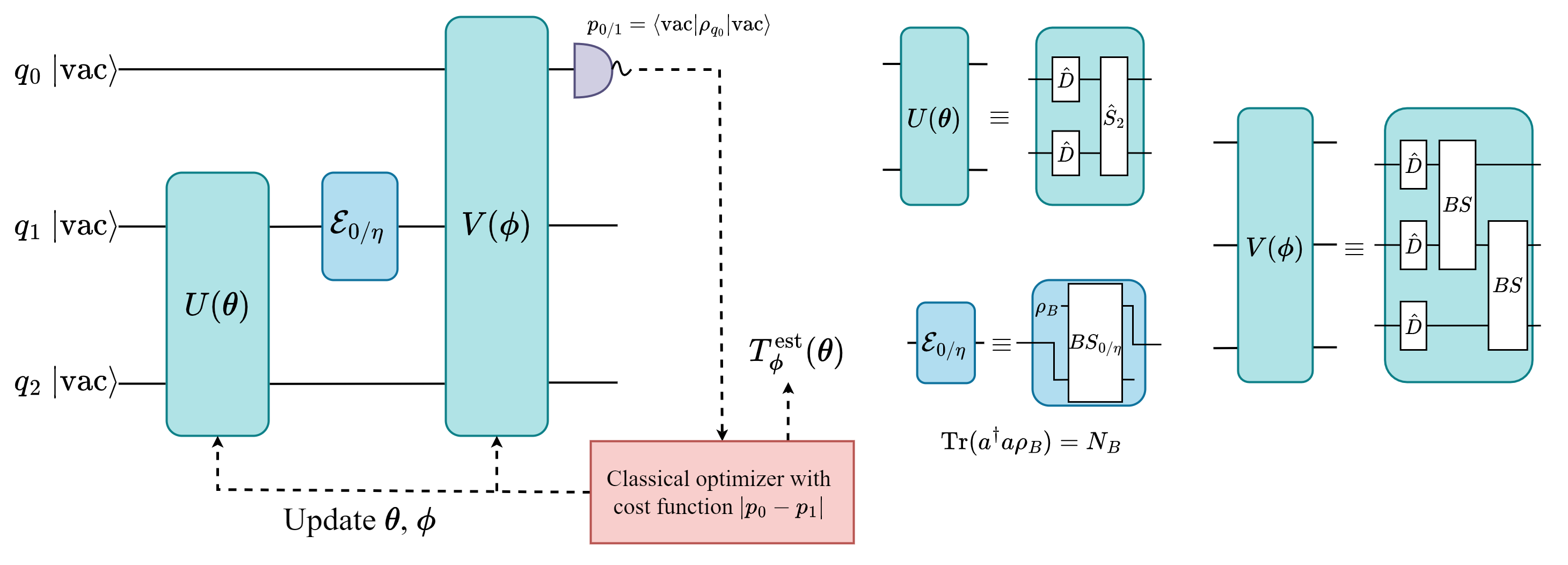
Figure 6: Description of the quantum circuit for variational quantum illumination. The state is prepared over the signal and idler mode using an ansatz which consists of displacements and two-mode squeezing. The ansatz shown for the measurement section consists of displacements and beam splitters. The simulations contain controlled phase gates for in the measurement section as well. The readout can be either measure the probability it is vacuum or the expectation value of the parity operator.

Appendix D Appendix D: Naimark dilation for Gaussian states

When we are working with purely Gaussian states, we have the limitation that the unitary $V$ must also be a Gaussian unitary. This puts a fundamental limitation on the form it can take, given that no two Gaussian states are orthogonal Ferraro et al. (2005). The overlap can be made as small as needed, but true orthogonality is impossible and hence we cannot reach the true canonical Naimark extension Paris (2012) if we choose to use only Gaussian operations. The isometry of the canonical Naimark extension in this case is given as follows which is not Gaussian.

$$V_{\mathrm{canonical}}=\mathbb{I}_{q_{0}}\otimes(\sqrt{\Gamma})_{SI}+i(-\outerproduct{0}{1}_{q_{0}}+\outerproduct{1}{0}_{q_{0}}+\mathbb{I}-\outerproduct{0}{0}-\outerproduct{1}{1})\otimes(\sqrt{\mathbb{I}-\Gamma})_{SI}$$ (20)

On the other hand, we can frame this as trying to perform a measurement on some $n$ mode state by entangling it to a 1 mode system. This can be written as follows.

$$\text{Tr}(V^{\dagger}(P_{0}\otimes\mathbb{I}_{n})V(\outerproduct{0}{0}\otimes\rho))=\text{Tr}(P\rho)$$ (21)

Here $P_{0}$ is a a projection which is in $L(\mathcal{H})$ where $\mathcal{H}$ is the Hilbert space of a single mode of light. $P$ is a projection in $L(\mathcal{H}^{\otimes n})$ and $\rho$ is a density operator in $D(\mathcal{H}^{\otimes n})$ and $\mathbb{I}_{n}$ is the identity operator in $L(\mathcal{H}^{\otimes n})$. Since we want the above equation to hold for all $\rho$, we can rewrite it as follows.

$$V^{\dagger}(P_{0}\otimes\mathbb{I}_{n})V=\mathbb{I}_{1}\otimes P$$ (22)

Here we are applying a transformation from one linear operator to another which means that as long as the norm of both $P_{0}\otimes\mathbb{I}_{n}$ and $\mathbb{I}_{1}\otimes P$ are equal, we can find a $V$. We can construct a $V=(\mathrm{SWAP}_{1,2}\otimes\mathbb{I}_{n-1})(\mathbb{I}_{1}\otimes V^{\prime})$ where it performs a swap between the first two modes and then does some unitary $V^{\prime}$ only on the subsystem of $n$ modes. This transforms the measurement from the space of the first mode to the space of the $n$ modes.

$$(\mathbb{I}_{1}\otimes V^{\prime})^{\dagger}(\mathrm{SWAP}_{1,2}\otimes\mathbb{I}_{n-1})^{\dagger}(P_{0}\otimes\mathbb{I}_{n})(\mathrm{SWAP}_{1,2}\otimes\mathbb{I}_{n-1})(\mathbb{I}_{1}\otimes V^{\prime})=\mathbb{I}_{1}\otimes V^{\prime\dagger}(P_{0}\otimes\mathbb{I}_{n-1})V^{\prime\dagger}$$ (23)

This shows that we can construct any projection of form $P=V^{\prime\dagger}(P_{0}\otimes\mathbb{I}_{n-1})V^{\prime\dagger}$ where $V^{\prime}$ is Gaussian since the swap operation between two modes can be trivially represented as a passive Gaussian operation. This recipe shows us that while we may not be able to construct the canonical Naimark extension of the optimal POVM, we can construct a Naimark extension that performs a POVM on the $n$ mode subspace using a single-mode ancillary measurement.

Appendix E Appendix E: Multiple optima in Gaussian quantum illumination

As can be seen in Fig. 2 of the main text, there are certain states which do not have 100% fidelity with the TMSV yet happen to have equal performance in the QFI, chernoff bound and the trace distance. These states are largely accessible due to the constraint only being placed on the value of signal photon number $N_{S}$.
We pick the example of the state obtained in the case of $N_{B}=1$. We perform a Schmidt decomposition on this state and compare it with the TMSV. Equal Schmidt values imply that one state can be obtained from the other using only local transformations implying equal entanglement as well. It turns out that this is not the case and the TMSV is different from the obtained optimal state despite both being equally good for the hypothesis testing task. This implies that there are clearly multiple possible Gaussian states which are optimal for the hypothesis testing task.

The five largest Schmidt values for TMSV with $N_{S}=0.1$ are $6.20921323\times 10^{-5},6.83013455\times 10^{-4},7.51314801\times 10^{-3},8.26446281\times 10^{-2},9.09090909\times 10^{-1}$. The TMSV has a von-Neumann entropy of $0.33509970612111517$.
The five largest Schmidt values for the obtained optimal state at $N_{B}=1$ with $N_{S}=0.1$ are $6.03874183\times 10^{-5},6.69019663\times 10^{-4},7.41192949\times 10^{-3},8.21152229\times 10^{-2},9.09737450\times 10^{-1}$. This state has a von-Neumann entropy of $0.3332223308457541$.

References

- Preskill (2018) J. Preskill, Quantum 2, 79 (2018).
- Bharti et al. (2022) K. Bharti, A. Cervera-Lierta, T. H. Kyaw, T. Haug, S. Alperin-Lea, A. Anand, M. Degroote, H. Heimonen, J. S. Kottmann, T. Menke, W.-K. Mok, S. Sim, L.-C. Kwek, and A. Aspuru-Guzik, Rev. Mod. Phys. 94, 015004 (2022).
- Cerezo et al. (2021a) M. Cerezo, A. Arrasmith, R. Babbush, S. C. Benjamin, S. Endo, K. Fujii, J. R. McClean, K. Mitarai, X. Yuan, L. Cincio, and P. J. Coles, Nature Reviews Physics 3, 625 (2021a).
- McClean et al. (2016) J. R. McClean, J. Romero, R. Babbush, and A. Aspuru-Guzik, New Journal of Physics 18, 023023 (2016).
- Farhi et al. (2014) E. Farhi, J. Goldstone, and S. Gutmann, “A quantum approximate optimization algorithm,” (2014), arXiv:1411.4028 [quant-ph] .
- McClean et al. (2018) J. R. McClean, S. Boixo, V. N. Smelyanskiy, R. Babbush, and H. Neven, Nature Communications 9, 4812 (2018).
- Wang et al. (2021) S. Wang, E. Fontana, M. Cerezo, K. Sharma, A. Sone, L. Cincio, and P. J. Coles, Nature Communications 12, 6961 (2021).
- Cerezo et al. (2021b) M. Cerezo, A. Sone, T. Volkoff, L. Cincio, and P. J. Coles, Nature Communications 12 (2021b), 10.1038/s41467-021-21728-w.
- Liu et al. (2023) H.-Y. Liu, T.-P. Sun, Y.-C. Wu, Y.-J. Han, and G.-P. Guo, New Journal of Physics 25, 013039 (2023).
- Kandala et al. (2017) A. Kandala, A. Mezzacapo, K. Temme, M. Takita, M. Brink, J. M. Chow, and J. M. Gambetta, Nature 549, 242–246 (2017).
- Peruzzo et al. (2014) A. Peruzzo, J. McClean, P. Shadbolt, M.-H. Yung, X.-Q. Zhou, P. J. Love, A. Aspuru-Guzik, and J. L. O’Brien, Nature Communications 5, 4213 (2014).
- Jones et al. (2019) T. Jones, S. Endo, S. McArdle, X. Yuan, and S. C. Benjamin, Phys. Rev. A 99, 062304 (2019).
- Kaubruegger et al. (2021) R. Kaubruegger, D. V. Vasilyev, M. Schulte, K. Hammerer, and P. Zoller, Phys. Rev. X 11, 041045 (2021).
- Marciniak et al. (2022) C. D. Marciniak, T. Feldker, I. Pogorelov, R. Kaubruegger, D. V. Vasilyev, R. van Bijnen, P. Schindler, P. Zoller, R. Blatt, and T. Monz, Nature 603, 604 (2022).
- Beckey et al. (2022) J. L. Beckey, M. Cerezo, A. Sone, and P. J. Coles, Phys. Rev. Research 4, 013083 (2022).
- Chen et al. (2021) R. Chen, Z. Song, X. Zhao, and X. Wang, Quantum Science and Technology 7, 015019 (2021).
- Lloyd (2008) S. Lloyd, Science 321, 1463 (2008).
- Shapiro and Lloyd (2009) J. H. Shapiro and S. Lloyd, New Journal of Physics 11, 063045 (2009).
- Tan et al. (2008) S.-H. Tan, B. I. Erkmen, V. Giovannetti, S. Guha, S. Lloyd, L. Maccone, S. Pirandola, and J. H. Shapiro, Physical Review Letters 101 (2008), 10.1103/physrevlett.101.253601.
- Sanz et al. (2017) M. Sanz, U. Las Heras, J. J. Garcia-Ripoll, E. Solano, and R. Di Candia, Phys. Rev. Lett. 118, 070803 (2017).
- Fan and Zubairy (2018) L. Fan and M. S. Zubairy, Phys. Rev. A 98, 012319 (2018).
- Lee et al. (2021) S.-Y. Lee, Y. S. Ihn, and Z. Kim, Phys. Rev. A 103, 012411 (2021).
- Karsa et al. (2020) A. Karsa, G. Spedalieri, Q. Zhuang, and S. Pirandola, Phys. Rev. Research 2, 023414 (2020).
- Aharonov et al. (1998) D. Aharonov, A. Kitaev, and N. Nisan, in Proceedings of the Thirtieth Annual ACM Symposium on Theory of Computing, STOC ’98 (Association for Computing Machinery, New York, NY, USA, 1998) p. 20–30.
- Harrow et al. (2010) A. W. Harrow, A. Hassidim, D. W. Leung, and J. Watrous, Phys. Rev. A 81, 032339 (2010).
- Bavaresco et al. (2021) J. Bavaresco, M. Murao, and M. T. Quintino, Phys. Rev. Lett. 127, 200504 (2021).
- Audenaert et al. (2007) K. M. R. Audenaert, J. Calsamiglia, R. Muñoz Tapia, E. Bagan, L. Masanes, A. Acin, and F. Verstraete, Phys. Rev. Lett. 98, 160501 (2007).
- Nussbaum and Szkoła (2009) M. Nussbaum and A. Szkoła, The Annals of Statistics 37, 1040 (2009).
- Li (2014) K. Li, The Annals of Statistics 42 (2014), 10.1214/13-aos1185.
- Hiai and Petz (1991) F. Hiai and D. Petz, Communications in Mathematical Physics 143, 99 (1991).
- Ogawa and Nagaoka (2000) T. Ogawa and H. Nagaoka, IEEE Transactions on Information Theory 46, 2428 (2000).
- Holevo (1973) A. S. Holevo, Problemy Peredachi Informatsii 9, 3 (1973).
- Helstrom (1969) C. W. Helstrom, Journal of Statistical Physics 1, 231 (1969).
- D’Ariano et al. (2001) G. M. D’Ariano, P. Lo Presti, and M. G. A. Paris, Phys. Rev. Lett. 87, 270404 (2001).
- Bae et al. (2019) J. Bae, D. Chruściński, and M. Piani, Phys. Rev. Lett. 122, 140404 (2019).
- Piani and Watrous (2009) M. Piani and J. Watrous, Phys. Rev. Lett. 102, 250501 (2009).
- Sacchi (2005) M. F. Sacchi, Phys. Rev. A 72, 014305 (2005).
- D’Ariano et al. (2003) G. M. D’Ariano, M. G. A. Paris, and M. F. Sacchi, “Quantum tomography,” (2003), arXiv:quant-ph/0302028 [quant-ph] .
- Watrous (2008) J. Watrous, “Quantum computational complexity,” (2008), arXiv:0804.3401 [quant-ph] .
- Agarwal et al. (2021) R. Agarwal, S. Rethinasamy, K. Sharma, and M. M. Wilde, “Estimating distinguishability measures on quantum computers,” (2021).
- Wilde (2013) M. M. Wilde, Proceedings of the Royal Society A: Mathematical, Physical and Engineering Sciences 469, 20130259 (2013).
- Lloyd and Montangero (2014) S. Lloyd and S. Montangero, Phys. Rev. Lett. 113, 010502 (2014).
- Bromley et al. (2020) T. R. Bromley, J. M. Arrazola, S. Jahangiri, J. Izaac, N. Quesada, A. D. Gran, M. Schuld, J. Swinarton, Z. Zabaneh, and N. Killoran, Quantum Science and Technology 5, 034010 (2020).
- Killoran et al. (2019) N. Killoran, J. Izaac, N. Quesada, V. Bergholm, M. Amy, and C. Weedbrook, Quantum 3, 129 (2019).
- Winter (2017) A. Winter, “Energy-constrained diamond norm with applications to the uniform continuity of continuous variable channel capacities,” (2017), arXiv:1712.10267 [quant-ph] .
- De Palma and Borregaard (2018) G. De Palma and J. Borregaard, Phys. Rev. A 98, 012101 (2018).
- Bradshaw et al. (2021) M. Bradshaw, L. O. Conlon, S. Tserkis, M. Gu, P. K. Lam, and S. M. Assad, Phys. Rev. A 103, 062413 (2021).
- Noh et al. (2021) C. Noh, C. Lee, and S.-Y. Lee, “Quantum illumination with non-gaussian states: Bounds on the minimum error probability using quantum fisher information,” (2021).
- Cariolaro and Pierobon (2016) G. Cariolaro and G. Pierobon, Phys. Rev. A 94, 062109 (2016).
- Buscemi et al. (2005) F. Buscemi, M. Keyl, G. M. D’Ariano, P. Perinotti, and R. F. Werner, Journal of Mathematical Physics 46, 082109 (2005).
- Tsang (2012) M. Tsang, Phys. Rev. Lett. 108, 170502 (2012).
- Scott and Nowak (2005) C. Scott and R. Nowak, IEEE Transactions on Information Theory 51, 3806 (2005).
- Huang et al. (2023) Z. Huang, C. Schwab, and C. Lupo, Phys. Rev. A 107, 022409 (2023).
- Tsang et al. (2016) M. Tsang, R. Nair, and X.-M. Lu, Phys. Rev. X 6, 031033 (2016).
- Chiribella et al. (2008a) G. Chiribella, G. M. D’Ariano, and P. Perinotti, Phys. Rev. Lett. 101, 180501 (2008a).
- Pirandola (2011) S. Pirandola, Phys. Rev. Lett. 106, 090504 (2011).
- Ortolano et al. (2021) G. Ortolano, E. Losero, S. Pirandola, M. Genovese, and I. Ruo-Berchera, Science Advances 7, eabc7796 (2021).
- Rosgen (2011) B. Rosgen, in Theory of Quantum Computation, Communication, and Cryptography, edited by W. van Dam, V. M. Kendon, and S. Severini (Springer Berlin Heidelberg, Berlin, Heidelberg, 2011) pp. 63–76.
- Beigi and Shor (2008) S. Beigi and P. W. Shor, “On the complexity of computing zero-error and holevo capacity of quantum channels,” (2008), arXiv:0709.2090 [quant-ph] .
- Janzing et al. (2005) D. Janzing, P. Wocjan, and T. Beth, International Journal of Quantum Information 03, 463 (2005).
- Chiribella et al. (2008b) G. Chiribella, G. M. D’Ariano, and P. Perinotti, Phys. Rev. Lett. 101, 060401 (2008b).
- Hirota (2020) O. Hirota, “Application of quantum pinsker inequality to quantum communications,” (2020).
- Spedalieri and Braunstein (2014) G. Spedalieri and S. L. Braunstein, Phys. Rev. A 90, 052307 (2014).

References

- Ben-Aroya and Ta-Shma (2009) A. Ben-Aroya and A. Ta-Shma, On the complexity of approximating the diamond norm (2009), arXiv:0902.3397 [quant-ph] .
- Benenti and Strini (2010) G. Benenti and G. Strini, Journal of Physics B: Atomic, Molecular and Optical Physics 43, 215508 (2010).
- Watrous (2008) J. Watrous, Distinguishing quantum operations having few kraus operators (2008), arXiv:0710.0902 [quant-ph] .
- Johansson et al. (2012) J. Johansson, P. Nation, and F. Nori, Computer Physics Communications 183, 1760 (2012).
- Johansson et al. (2013) J. Johansson, P. Nation, and F. Nori, Computer Physics Communications 184, 1234 (2013).
- Kandala et al. (2017) A. Kandala, A. Mezzacapo, K. Temme, M. Takita, M. Brink, J. M. Chow, and J. M. Gambetta, Nature 549, 242–246 (2017).
- Lloyd and Montangero (2014) S. Lloyd and S. Montangero, Phys. Rev. Lett. 113, 010502 (2014).
- Aharonov et al. (1998) D. Aharonov, A. Kitaev, and N. Nisan, in Proceedings of the Thirtieth Annual ACM Symposium on Theory of Computing, STOC ’98 (Association for Computing Machinery, New York, NY, USA, 1998) p. 20–30.
- Chen et al. (2021) R. Chen, Z. Song, X. Zhao, and X. Wang, Quantum Science and Technology 7, 015019 (2021).
- Agarwal et al. (2021) R. Agarwal, S. Rethinasamy, K. Sharma, and M. M. Wilde, Estimating distinguishability measures on quantum computers (2021).
- Wilde (2013) M. M. Wilde, Proceedings of the Royal Society A: Mathematical, Physical and Engineering Sciences 469, 20130259 (2013).
- Holevo (1973) A. S. Holevo, Problemy Peredachi Informatsii 9, 3 (1973).
- Helstrom (1969) C. W. Helstrom, Journal of Statistical Physics 1, 231 (1969).
- Ferraro et al. (2005) A. Ferraro, S. Olivares, and M. G. A. Paris, Gaussian states in continuous variable quantum information (2005), arXiv:quant-ph/0503237 [quant-ph] .
- Paris (2012) M. G. A. Paris, The European Physical Journal Special Topics 203, 61 (2012).