A massless interacting Fermionic Cellular Automaton exhibiting bound states

Abstract

We present a Fermionic Cellular Automaton model which describes massless Dirac fermion in $1+1$ dimension coupled with local, number preserving interaction. The diagonalization of the two particle sector shows that specific values of the total momentum and of the coupling constant allows for the formation of bound states.

I Introduction

Quantum cellular automata (QCAs)Farrelly (2020); Arrighi (2019); Schumacher and Werner (2004); Gross et al. (2012) are the most general unitary dynamics of a lattice of quantum systems which is discrete in time and causal, namely the speed of information propagation is bounded. The idea of QCAs can be traced back to the seminal work of Feynman Feynman (1982) where QCAs were introduced as quantum simulators. Since then, QCAs have been considered as a paradigm for quantum computationWatrous (1995); Raussendorf (2005); Childs (2009); Lovett et al. (2010) and have been applied to the study of many bodies quantum systems Cirac et al. (2017); Po et al. (2016); Haah et al. (2023); Piroli and Cirac (2020); Zimborás et al. (2022); Hillberry et al. (2021).

Nevertheless, quantum simulation still is a major application of QCAs, in particular as discretized quantum field theories. Many authors Bialynicki-Birula (1994); Meyer (1996); Strauch (2006); Yepez (2006); D’Ariano and Perinotti (2014); Arrighi et al. (2014); Bisio et al. (2015, 2016); Arrighi et al. (2018) studied the simulation of non-interacting quantum field theories with discrete-time Quantum Walks (QWs) Ambainis et al. (2001); Portugal (2013), which are the single-particle restriction of Bosonic QCAs or Fermionic Cellular Automata (FCA)—a variation of QCAs where the cells correspond to arrays of local Fermionic modes Bravyi and Kitaev (2002). Indeed, a QW describes the most general time-discrete evolution of a single particle on a lattice which is unitary and causal, i.e. at each step the particle can move at most by a bounded number of lattice sites. More recently, the focus shifted towards to models in which the particles interact with an external potential Bisio et al. (2013); Di Molfetta et al. (2013); Arnault and Debbasch (2016); Jay et al. (2020) and towards interacting field theories Bisio et al. (2018); Eon et al. (2022).

Intuitively, we expect that a QCA/FCA which simulates (or recovers) a given continuous dynamics is such that, if we restrict to sufficiently smeared states which cannot probe the discreteness of the lattice, we cannot tell the evolution apart from the dynamics of a field on a continuous space. For the non-interacting case this behaviour is rather well understood. In the limit of small masses and momentum ($m,k\to 0$), and interpolating discrete time steps with a continuous time direction, the evolution of the cellular automaton is described by a relativistic wave equation. The interacting case, still rather unexplored, is significantly different. The intrinsic discreteness of cellular automata may produce phenomenological features with no counterpart in the continuum and that do not vanish in the large scale limit, like a different set of bound states and scattering processes that conserve energy only up to integer multiples of an additive constant (indeed, if time is discrete energy is periodic) Bisio et al. (2018, 2021).

In this work we present an interacting FCA which describes the evolution of a massless Dirac spinor in $1+1$-dimensional spacetime. The FCA is given by the composition of a free evolution, which is modeled after the massless Dirac equation D’Ariano and Perinotti (2014) followed by a quartic, number preserving local interaction. We will study the evolution of the two particle sector by providing the spectral resolution of the unitary evolution corresponding to a single step of the FCA. Our analysis will show that, even if the free theory is gapless and the interaction is a compact perturbation, bound states appear for critical values of the total momentum and of the coupling constant.

In section II we review the technical tools employed for QCAs and QWs and provide a mathematical description of the Dirac automaton. In section III we describe the interaction considered and its properties, then we derive the scattering and the bounded states of the system. In appendices A and B we check the completeness of the solution set.

II Fermionic Cellular Automata

A quantum cellular automaton (QCA) describes the single step unitary evolution $\mathcal{U}$ of a lattice of cells each of which represents a quantum system. The QCA evolution must be local, i.e. the state of cell $x$ at time $t$ must depend only on the state of the cells which belongs to a finite neighborhood $N_{x}$ at time $t-1$ (see Fig.1). In the Heisenberg picture, local observables at site $X$ at time step $t$ are mapped to local observables in finite neighborhood $N_{x}$ at step $t-1$. QCAs aimed at recovering a field theory in the continuum are homogeneous (or translation-invariant), namely $i)$ the quantum systems corresponding to the cells of the lattice are all isomorphic, and $ii)$ the evolution commutes with the group of translations on the lattice. For Quantum Cellular Automata every cell consists in a $d$-level system. In the present paper, however, we will focus on FCAs, where every cell corresponds to a set of local Fermionic modes Kitaev (1997); D’Ariano et al. (2014).

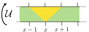
Figure 1: (Colors online) In a one-dimensional cellular automaton each cell is labelled by an integer number $x$ and the one-step time evolution is described by a unitary operator $\mathcal{U}$. In a nearest-neighbor one-dimensional QCA the state of the cell $x$ at time $t+1$ depends only on the state of the cells $x-1$, $x$ and $x+1$ at time $t$. Because of the locality of the evolution, information cannot propagate at an arbitrary speed: physical interventions on cell $x$ can only affect the state of the cells lying in the future light cone of $x$ (in yellow).

For our purposes, we consider the case in which the lattice is one dimensional (i.e. an infinite chain of cells) and each cell contains $S$ fermionic modes . Therefore, each cell is labelled by an integer number $x\in\mathbb{Z}$ and at each cell $x$ we have $S$ fermionic modes represented by the field operators $\psi_{x,a}$, $a=1,\dots,S$ obeying the canonical anticommutation relations:

$$\{\psi_{x,a},\psi_{x^{\prime},a^{\prime}}\}=0,\quad\{\psi_{x,a},\psi_{x^{\prime},a^{\prime}}^{\dagger}\}=\delta_{x,x^{\prime}}\delta_{a,a^{\prime}}.$$ (1)

If $\tau$ denotes the translation operator on the infinite chain, i.e. $\tau(\psi_{x,a})=\psi_{x+1,a}$, the homogeneity of the evolution is equivalent to the commutation relation $\tau\circ\mathcal{U}=\mathcal{U}\circ\tau$. We consider nearest-neighbor cellular automata, namely $N_{x}\coloneqq\{x-1,x,x+1\}$.

The $N$-particles states can be described by introducing the Fock space representation $|(x_{1},a_{1}),\ldots,(x_{N},a_{N})\rangle\coloneqq\psi^{\dagger}_{x_{1},a_{1}}\ldots\psi^{\dagger}_{x_{N},a_{N}}|\Omega\rangle$, where $|\Omega\rangle$ is the vacuum state. The state $|\Omega\rangle$ is defined by the identity $\psi_{x,a}|\Omega\rangle=0$ for all $i$ and it is the state with no particles. Here, we chose the representation in which the vacuum state is the one with no localized excitations, whereas in quantum field theory the vacuum state is usually the ground state of a free Hamiltonian.

If we consider the particular case of a free, i.e. non-interacting, evolution, the FCA evolution is linear in the field operators, namely $\mathcal{U}(\psi^{\dagger}_{x,a})=\sum_{y,b}U^{y,b}_{x,a}\psi_{y,b}$ for some complex coefficents $U_{x,a}^{y,b}$. For a nearest-neighbor, one-dimensional linear FCA we have $U_{x,a}^{y,b}=0$ if $|x-y|>1$ and $U_{x,a}^{y,b}=U_{0,a}^{y-x,b}$, where the last condition follows from translation invariance. The most general nearest-neighbor, one-dimensional linear Fermionic cellular automaton can be written as follows:

$$\begin{aligned} \psi^{\dagger}_{x}(t+1)&=\mathbf{U}_{-1}\psi^{\dagger}_{x-1}(t)+\mathbf{U}_{0}\psi^{\dagger}_{x}(t)+\mathbf{U}_{1}\psi^{\dagger}_{x+1}(t),\\ \psi^{\dagger}_{x}(t)&\coloneqq(\psi^{\dagger}_{x,1}(t),\dots,\psi^{\dagger}_{x,S}(t))^{T},\end{aligned}$$ (2)

where we introduced the $S\times S$ matrices $(\mathbf{U}_{j})^{a}_{b}\coloneqq U_{0,a}^{j,b}$. Because of translation invariance, the dynamics of this linear FCA is easily studied in terms of delocalised modes corresponding to plane waves, obtained as the Fourier transform of the local modes $\psi^{\dagger}_{k,a}\coloneqq\sum_{x}e^{-ikx}\psi^{\dagger}_{x,a}$, $k\in[-\pi,\pi)$. Then, Equation (2) becomes

$$\begin{aligned} \psi^{\dagger}_{k}(t+1)&=\mathbf{U}(k)\psi^{\dagger}_{k}(t),\\ \psi^{\dagger}_{k}(t)&\coloneqq(\psi^{\dagger}_{k,1}(t),\dots,\psi^{\dagger}_{k,S}(t))^{T},\\ (\mathbf{U}(k))^{a}_{b}&\coloneqq\sum_{n\in\{-1,0,1\}}e^{ink}(\mathbf{U}_{n})^{a}_{b},\end{aligned}$$ (3)

where the $S\times S$ matrix $\mathbf{U}(k)$ must be unitary.

In a linear FCA the number of excitations (i.e. particles) is conserved and the dynamics is completely specified by the one-particle sector $\mathcal{H}_{1}\coloneqq\operatorname{span}\{|x,a\rangle\}\equiv\mathbb{C}^{S}\otimes\ell^{2}(\mathbb{Z})$, where we implicitly adopt the isomorphism $|x,a\rangle\mapsto|a\rangle|x\rangle$. A generic one-particle state can be written as $|\phi\rangle=\sum_{a\in S,x\in\mathbb{Z}}c_{a,x}|a\rangle|x\rangle=\int_{-\pi}^{\pi}dk\tilde{c}_{a,k}|a\rangle|k\rangle$ with $|k\rangle\coloneqq\sum_{x\in\mathbb{Z}}e^{-ikx}|x\rangle$ and $\tilde{c}_{a,k}\coloneqq\sum_{x\in\mathbb{Z}}e^{ikx}c_{a,x}$. Then, the one particle sector of a linear FCA $\mathcal{U}$ is described by the quantum walk

$$\begin{aligned} &|\phi(t+1)\rangle\coloneqq\mathbf{U}|\phi(t)\rangle,\\ &\mathbf{U}\coloneqq\int_{-\pi}^{\pi}dk\mathbf{U}(k)\otimes|k\rangle\langle k|.\end{aligned}$$ (4)

Accordingly, the $n$-particle sector of a linear FCA $\mathcal{U}$ is described by the total antisymmetric subspace of the $n$-particle quantum walk $\mathbf{U}^{\otimes{n}}$. Therefore, a linear FCA can be regarded as the second-quantization of a Quantum Walk.

Let us consider the following linear FCA which evolves a four component fermionic field on a one dimensional lattice:

$$\psi^{\dagger}_{k}(t+1) =\mathbf{D}_{m}(k)\psi^{\dagger}_{k}(t),$$ (5)

$$\psi^{\dagger}_{k}(t) \coloneqq(\psi^{\dagger}_{k,1}(t),\psi^{\dagger}_{k,2}(t),\psi^{\dagger}_{k,3}(t),\psi^{\dagger}_{k,4}(t))^{T},$$

$$\mathbf{D}_{m}(k) \coloneqq\begin{pmatrix}e^{-ik}&0&-im&0\\ 0&e^{ik}&0&-im\\ -im&0&e^{ik}&0\\ 0&-im&0&e^{-ik}\\ \end{pmatrix}.$$ (6)

One can prove Bisio et al. (2015); Chandrashekar et al. (2010) that, in the $k,m\to 0$ limit, this evolution recovers the one dimensional Dirac equation for a spinor with mass $m$. For this reason the above cellular automaton is referred to as Dirac cellular automaton.

III FCA with local interaction

Here we consider a discrete version of a gauge theory where a linear FCA is followed by a local change of basis without breaking the translation invariance. The local change of basis models the arbitrariness of the identification of local bases at subsequent discrete time steps. While in quantum field theory the local gauge symmetry is ruled by a classical field which is quantized in a second stage, here we preserve translation invariance, with the implicit goal of identifying the quantized gauge fields with suitable degrees of freedom of the Fermionic fields already at hand.

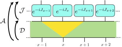
Figure 2: (Colors online) The single step evolution of the FCA of Equation (7). Each site of the lattice corresponds to a four-component fermionic field. The free evolution $\mathcal{D}$ involves the nearest neighbors while the interaction $\mathcal{J}$ is completely local.

We thus consider a FCA model $\mathcal{A}$ of the form (see Fig. 2)

$$\mathcal{A}\coloneqq\mathcal{J}\circ\mathcal{D},$$ (7)

where $\mathcal{D}$ is the linear FCA defined in Equation (5) for $m=0$ and

$$\mathcal{J}\big{(}\psi_{x,a}\big{)}\coloneqq\exp(-i\sum_{x}J_{x})\psi_{x,a}\exp\big{(}i\sum_{x}J_{x}\big{)},$$ (8)

$$\begin{aligned} &J_{x}\coloneqq\lambda O_{x}+\overline{\lambda}O^{\dagger}_{x},\qquad\lambda\in\mathbb{C},\\ &O_{x}\coloneqq\psi_{x,2}\psi^{\dagger}_{x,3}\psi_{x,3}\psi^{\dagger}_{x,4}+\psi_{x,1}\psi^{\dagger}_{x,3}\psi^{\dagger}_{x,4}\psi_{x,4}\,.\end{aligned}$$

Since $\mathcal{A}$ is number preserving, we can analyze its dynamics for fixed number of particles. Our goal is to diagonalize the evolution in the two particle sector. Since we are dealing with a Fermionic system, the two particle Hilbert space is given by the antisymmetric subspace $\mathcal{H}_{-}$ of the tensor product $\mathcal{H}_{1}\otimes\mathcal{H}_{1}$ of two copies of the one particle space $\mathcal{H}_{1}=\operatorname{span}\big{\{}|a\rangle|x\rangle\big{\}}\equiv\mathbb{C}^{4}\otimes\ell^{2}(\mathbb{Z})$ , where $a\in\{1,2,3,4\}$ and $x\in\mathbb{Z}$. Namely, we have

$$\begin{aligned} \mathcal{H}_{-}\coloneqq\operatorname{supp}\mathbf{P}_{-},\quad\mathbf{P}_{-}\coloneqq\frac{1}{2}\big{(}\mathbf{I}-\mathbf{S}\big{)},\end{aligned}$$ (9)

where $\mathbf{I}$ is the identity on $\mathcal{H}_{1}\otimes\mathcal{H}_{1}$ and $\mathbf{S}$ is the swap operator $\mathbf{S}|a_{1}\rangle|a_{2}\rangle|x_{1}\rangle|x_{2}\rangle=|a_{2}\rangle|a_{1}\rangle|x_{2}\rangle|x_{1}\rangle$, where

$$\begin{aligned} &\mathcal{H}_{1}\otimes\mathcal{H}_{1}=\operatorname{span}\big{\{}|a_{1}\rangle|a_{2}\rangle|x_{1}\rangle|x_{2}\rangle\big{\}},\\ &\,a_{1},a_{2}\in\{1,2,3,4\},\quad x_{1},x_{2}\in\mathbb{Z}.\end{aligned}$$ (10)

Then, the two-particle sector of $\mathcal{D}$ is described by the unitary operator $\mathbf{D}_{2}\coloneqq\mathbf{P}_{-}\,\big{(}\mathbf{D}\otimes\mathbf{D}\big{)}\,\mathbf{P}_{-}$ where $\mathbf{D}\in\mathcal{L}(\mathcal{H}_{1})$ is given by Equation (5) with $m=0$. Moreover, from a straightforward computation it follows that the two-particle sector of $\mathcal{J}$ is described by the unitary operator $\mathbf{J}_{2}\coloneqq\mathbf{P}_{-}\mathbf{J}\mathbf{P}_{-}$, where

$$\begin{aligned} &\mathbf{J}\coloneqq\exp\big{(}-i\sum_{x}\mathbf{J}_{x}\big{)},\\ &\mathbf{J}_{x}\coloneqq\big{(}\lambda\mathbf{O}+\overline{\lambda}\mathbf{O}^{\dagger}\big{)}\otimes|x\rangle\langle x|\otimes|x\rangle\langle x|\\ &\begin{aligned} \mathbf{O}\coloneqq&|3\rangle\langle 1|\otimes|4\rangle\langle 4|+|3\rangle\langle 3|\otimes|4\rangle\langle 2|+\\ &+|4\rangle\langle 2|\otimes|3\rangle\langle 3|+|4\rangle\langle 4|\otimes|3\rangle\langle 1|\,.\end{aligned}\end{aligned}$$ (11)

Since $[\mathbf{D}\otimes\mathbf{D},\mathbf{P}_{-}]=[\mathbf{J},\mathbf{P}_{-}]=0$, we have that the two-particle sector of $\mathcal{A}$ is described by the operator

$$\mathbf{A}_{2}\coloneqq\mathbf{P}_{-}\,\Big{(}\mathbf{J}\,(\mathbf{D}\otimes\mathbf{D})\Big{)}\,\mathbf{P}_{-}.$$ (12)

Therefore, the goal of this section is to diagonalize the operator $\mathbf{A}_{2}$. Let us now define

$$\mathbf{Q}\coloneqq\mathbf{Q}^{\prime}\otimes\mathbf{I}\otimes\mathbf{I}$$ (13)

$$\begin{aligned} \mathbf{Q}^{\prime}\coloneqq&|2\rangle\langle 2|\otimes|3\rangle\langle 3|+|3\rangle\langle 3|\otimes|2\rangle\langle 2|+\\ +&|3\rangle\langle 3|\otimes|4\rangle\langle 4|+|4\rangle\langle 4|\otimes|3\rangle\langle 3|+\\ +&|1\rangle\langle 1|\otimes|4\rangle\langle 4|+|4\rangle\langle 4|\otimes|1\rangle\langle 1|.\end{aligned}$$ (14)

From a straightworward computation we have $[\mathbf{A}_{2},\mathbf{Q}]=0$ an therefore we can write

$$\begin{aligned} &\mathbf{A}_{2}\coloneqq\widetilde{\mathbf{A}}_{2}\oplus\widetilde{\mathbf{A}}^{\perp}_{2}\,\\ &\widetilde{\mathbf{A}}_{2},\coloneqq\mathbf{Q}\mathbf{A}_{2}\mathbf{Q},\qquad\widetilde{\mathbf{A}}^{\perp}_{2}\coloneqq(\mathbf{I}-\mathbf{Q})\mathbf{A}_{2}(\mathbf{I}-\mathbf{Q}).\end{aligned}$$ (15)

Since $\mathbf{Q}\mathbf{J}=\mathbf{J}\mathbf{Q}=0$, we have that $\widetilde{\mathbf{A}}^{\perp}_{2}$ is a free evolution. Therefore, we focus our analysis on the non trivial term $\widetilde{\mathbf{A}}_{2}$. Let us define the vectors

$$\begin{aligned} |e_{1}\rangle\coloneqq|1\rangle|4\rangle\quad|e_{2}\rangle\coloneqq|3\rangle|2\rangle\quad|e_{3}\rangle\coloneqq|3\rangle|4\rangle\\ |e_{4}\rangle\coloneqq|4\rangle|1\rangle\quad|e_{5}\rangle\coloneqq|2\rangle|3\rangle\quad|e_{6}\rangle\coloneqq|4\rangle|3\rangle\end{aligned}$$ (16)

and the Hilbert space $\widetilde{\mathcal{H}}\coloneqq\operatorname{span}\{|e_{i}\rangle,\}$. In the basis of Eq. (16), we have:

$$\lambda\mathbf{O}+\overline{\lambda}\mathbf{O}^{\dagger}=\begin{pmatrix}{\mathbf{O}}^{\prime}&\mathbf{0}\\ \mathbf{0}&{\mathbf{O}}^{\prime}\end{pmatrix},\qquad{\mathbf{O}}^{\prime}\coloneqq\begin{pmatrix}0&0&-\bar{\lambda}\\ 0&0&-\bar{\lambda}\\ -\lambda&-\lambda&0\\ \end{pmatrix}.$$ (17)

If we consider the total translation operator

$$\mathbf{T}_{2}|e_{i}\rangle|x_{1}\rangle|x_{2}\rangle=|e_{i}\rangle|x_{1}+1\rangle|x_{2}+1\rangle$$ (18)

it is straightforward to verify the commutation relation $[\mathbf{T}_{2},\widetilde{\mathbf{A}}_{2}]=0$. Therefore, it is convenient to introduce the relative coordinate basis

$$|e_{i}\rangle|x_{1}\rangle|x_{2}\rangle\mapsto|e_{i}\rangle|y\rangle|z\rangle$$ (19)

$$y\coloneqq x_{1}-x_{2}\quad z\coloneqq x_{1}+x_{2}$$ (20)

and to Fourier transform the $z$ coordinate, i.e.

$$|e_{i}\rangle|y\rangle|p\rangle\coloneqq|e_{i}\rangle|y\rangle\sum_{z\in\mathbb{Z}}e^{-ipz}|z\rangle.$$ (21)

In this basis, the operator $\widetilde{\mathbf{A}}_{2}$ can be written as follows:

$$\widetilde{\mathbf{A}}_{2}=\int_{-\pi}^{\pi}\!\!\!dp\,\,\,\widetilde{\mathbf{A}}_{2}(p)\otimes|p\rangle\langle p|,$$ (22)

$$\widetilde{\mathbf{A}}_{2}(p)\coloneqq\widetilde{\mathbf{P}}_{-}\,\widetilde{\mathbf{J}}\,\widetilde{\mathbf{D}}_{p}\,\widetilde{\mathbf{P}}_{-},$$ (23)

$$\widetilde{\mathbf{J}}\coloneqq\exp\left(-i\begin{pmatrix}{\mathbf{O}}^{\prime}&\mathbf{0}\\ \mathbf{0}&{\mathbf{O}}^{\prime}\end{pmatrix}\otimes|0\rangle\langle 0|\right),$$ (24)

$$\widetilde{\mathbf{D}}_{p}\coloneqq\begin{pmatrix}e^{2ip}&0&0&0&0&0\\ 0&e^{-2ip}&0&0&0&0\\ 0&0&\mathbf{T}_{y}^{\dagger 2}&0&0&0\\ 0&0&0&e^{2ip}&0&0\\ 0&0&0&0&e^{-2ip}&0\\ 0&0&0&0&0&\mathbf{T}_{y}^{2}\\ \end{pmatrix},$$ (25)

$$\widetilde{\mathbf{P}}_{-}\coloneqq\frac{1}{2}\left(\mathbf{I}\otimes\mathbf{I}-\begin{pmatrix}{\mathbf{0}}&\mathbf{I}\\ \mathbf{I}&{\mathbf{0}}\end{pmatrix}\otimes\sum_{y}|-y\rangle\langle y|\right).$$ (26)

Since the eigenvalues of ${\mathbf{O}}^{\prime}$ are $0,\pm\sqrt{2}|\lambda|$ we have that $\widetilde{\mathbf{J}}$ is the identity if $\sqrt{2}|\lambda|$ is an integer multiple of $2\pi$. Therefore, we will assume that $\sqrt{2}|\lambda|\neq 2n\pi$ ($n\in\mathbb{Z}$). Then, we can focus on the diagonalization of the (infinite-dimensional) operator $\widetilde{\mathbf{A}}_{2}(p)$. Let us now consider the following subspaces (see also Fig. 3):

$$\begin{aligned} &\widetilde{\mathcal{H}}_{a}\coloneqq\operatorname{span}\{|e_{1}\rangle|y\rangle-|e_{4}\rangle|-y\rangle,y\neq 0\},\\ &\widetilde{\mathcal{H}}_{b}\coloneqq\operatorname{span}\{|e_{2}\rangle|y\rangle-|e_{5}\rangle|-y\rangle,y\neq 0\},\\ &\widetilde{\mathcal{H}}_{c}\coloneqq\operatorname{span}\{|e_{3}\rangle|2y+1\rangle-|e_{6}\rangle|-2y-1\rangle\},\\ &\widetilde{\mathcal{H}}_{d}\coloneqq\big{(}\widetilde{\mathcal{H}}_{a}\oplus\widetilde{\mathcal{H}}_{b}\oplus\widetilde{\mathcal{H}}_{c}\big{)}^{\perp}.\end{aligned}$$ (27)

We remark that

$$\operatorname{supp}\widetilde{\mathbf{P}}_{-}= \widetilde{\mathcal{H}}_{a}\oplus\widetilde{\mathcal{H}}_{b}\oplus\widetilde{\mathcal{H}}_{c}\oplus\widetilde{\mathcal{H}}_{d}.$$ (28)

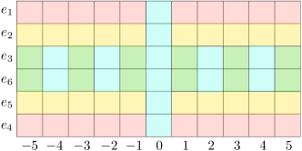
Figure 3: (Colors online) Schematic representation of the decomposition of Equation (27). On the horizontal axis we have the spatial degrees of freedom, on the vertical axis the internal ones. $\widetilde{\mathcal{H}}_{a}$ corresponds to the red region, $\widetilde{\mathcal{H}}_{b}$ corresponds to the yellow region, $\widetilde{\mathcal{H}}_{c}$ corresponds to the green region and $\widetilde{\mathcal{H}}_{d}$ corresponds to the blue region. Only states whose support is in $\widetilde{\mathcal{H}}_{d}$ are affected by the interaction.

We are now ready to proceed with the derivation of the spectral resolution of $\widetilde{\mathbf{A}}_{2}(p)$. For the sake of clarity, we split the proof into several lemmas.

Lemma 1.

Let $\widetilde{\mathbf{A}}_{2}(p)$ be defined as in Equation (23). Then we have

$$\begin{aligned} \widetilde{\mathbf{A}}_{2}(p)&=e^{i2p}\widetilde{\mathbf{P}}_{a}+e^{-i2p}\widetilde{\mathbf{P}}_{b}+\\ &+\widetilde{\mathbf{P}}_{c}\widetilde{\mathbf{A}}_{2}(p)\widetilde{\mathbf{P}}_{c}+\widetilde{\mathbf{P}}_{d}\widetilde{\mathbf{A}}_{2}(p)\widetilde{\mathbf{P}}_{d}\end{aligned}$$ (29)

where $\widetilde{\mathbf{P}}_{i}$, denotes the orthogonal projector on $\widetilde{\mathcal{H}}_{i}$.

Proof.

The subspaces $\widetilde{\mathcal{H}}_{i}$ in Equation (27) are invariant subspaces of $\widetilde{\mathbf{A}}_{2}(p)$. One can directly verify that $\widetilde{\mathbf{P}}_{a}\widetilde{\mathbf{A}}_{2}(p)\widetilde{\mathbf{P}}_{a}=e^{i2p}\widetilde{\mathbf{P}}_{a}$ and $\widetilde{\mathbf{P}}_{b}\widetilde{\mathbf{A}}_{2}(p)\widetilde{\mathbf{P}}_{b}=e^{-i2p}\widetilde{\mathbf{P}}_{b}$. $\,\blacksquare$

Lemma 2.

The operator $\widetilde{\mathbf{P}}_{c}\widetilde{\mathbf{A}}_{2}(p)\widetilde{\mathbf{P}}_{c}$ has the following spectral resolution:

$$\begin{aligned} \widetilde{\mathbf{P}}_{c}\widetilde{\mathbf{A}}_{2}(p)\widetilde{\mathbf{P}}_{c}&=\int_{-\pi}^{\pi}\!\!\!\!dk\,e^{-ik}|\phi_{f}(k)\rangle\langle\phi_{f}(k)|,\\ |\phi_{f}(k)\rangle&\coloneqq\frac{1}{\sqrt{2}}\big{(}|e_{3}\rangle|k\rangle_{o}-|e_{6}\rangle|-k\rangle_{o}\big{)}\\ |k\rangle_{o}&\coloneqq\sum_{y\in\mathbb{Z}}\frac{1}{\sqrt{2\pi}}e^{-iky}|2y+1\rangle.\end{aligned}$$ (30)

Proof.

We have $\widetilde{\mathbf{P}}_{c}\widetilde{\mathbf{A}}_{2}(p)\widetilde{\mathbf{P}}_{c}=\widetilde{\mathbf{P}}_{c}\,\widetilde{\mathbf{J}}\,\widetilde{\mathbf{D}}_{p}\,\widetilde{\mathbf{P}}_{c}$ Let us define the subspace $\ell^{2}(2\mathbb{Z}+1)\coloneqq\operatorname{span}{\{|2y+1\rangle,y\in\mathbb{Z}\}}\subset\ell^{2}(\mathbb{Z})$ and let us denote with $\widetilde{\mathbf{P}}_{\mathrm{odd}}$ the projector on $\ell^{2}(2\mathbb{Z}+1)$. It is easy to verify that $\widetilde{\mathbf{P}}_{c}\big{(}\mathbf{I}\otimes\widetilde{\mathbf{P}}_{\mathrm{odd}}\big{)}=\big{(}\mathbf{I}\otimes\widetilde{\mathbf{P}}_{\mathrm{odd}}\big{)}\widetilde{\mathbf{P}}_{c}=\widetilde{\mathbf{P}}_{c}$. Since $\widetilde{\mathbf{J}}$ is localized at the origin, we have that

$$\widetilde{\mathbf{P}}_{c}\,\widetilde{\mathbf{J}}\,\widetilde{\mathbf{D}}_{p}\,\widetilde{\mathbf{P}}_{c}= \widetilde{\mathbf{P}}_{c}\,\big{(}\mathbf{I}\otimes\widetilde{\mathbf{P}}_{\mathrm{odd}}\big{)}\,\widetilde{\mathbf{J}}\,\widetilde{\mathbf{D}}_{p}\,\big{(}\mathbf{I}\otimes\widetilde{\mathbf{P}}_{\mathrm{odd}}\big{)}\,\widetilde{\mathbf{P}}_{c}=$$

$$= \widetilde{\mathbf{P}}_{c}\,\big{(}\mathbf{I}\otimes\widetilde{\mathbf{P}}_{\mathrm{odd}}\big{)}\,\widetilde{\mathbf{D}}_{p}\,\big{(}\mathbf{I}\otimes\widetilde{\mathbf{P}}_{\mathrm{odd}}\big{)}\,\widetilde{\mathbf{P}}_{c}=$$

$$= \widetilde{\mathbf{P}}_{c}\,\big{(}|e_{3}\rangle\langle e_{3}|\otimes\mathbf{P}_{\mathrm{odd}}\mathbf{T}^{{\dagger}2}_{y}\mathbf{P}_{\mathrm{odd}}\big{)}\widetilde{\mathbf{P}}_{c}+$$

$$+\widetilde{\mathbf{P}}_{c}\,\big{(}|e_{6}\rangle\langle e_{6}|\otimes\mathbf{P}_{\mathrm{odd}}\mathbf{T}^{2}_{y}\mathbf{P}_{\mathrm{odd}}\big{)}\widetilde{\mathbf{P}}_{c}$$

The operator $\mathbf{P}_{\mathrm{odd}}\mathbf{T}^{2}_{y}\mathbf{P}_{\mathrm{odd}}$ is easily diagonalized as follows:

$$\mathbf{P}_{\mathrm{odd}}\mathbf{T}^{2}_{y}\mathbf{P}_{\mathrm{odd}}=\int_{-\pi}^{\pi}\!\!\!dk\,e^{-ik}|k\rangle_{o}\langle k|_{o}.$$

Then we have

$$|e_{3}\rangle\langle e_{3}|\otimes\mathbf{P}_{\mathrm{odd}}\mathbf{T}^{{\dagger}2}_{y}\mathbf{P}_{\mathrm{odd}}+|e_{6}\rangle\langle e_{6}|\otimes\mathbf{P}_{\mathrm{odd}}\mathbf{T}^{2}_{y}\mathbf{P}_{\mathrm{odd}}=$$

$$=\int_{-\pi}^{\pi}\!\!\!\!dk\,e^{-ik}\big{(}|e_{3}\rangle\langle e_{3}|\otimes|k\rangle_{o}\langle k|_{o}+|e_{6}\rangle\langle e_{6}|\otimes|-k\rangle_{o}\langle-k|_{o}\big{)}.$$

Since $\widetilde{\mathbf{P}}_{c}|e_{3}\rangle|k\rangle_{o}=-\widetilde{\mathbf{P}}_{c}|e_{6}\rangle|-k\rangle_{o}=1/\sqrt{2}|\phi_{f}(k)\rangle$ we have the thesis. $\,\blacksquare$

Lemma 3.

We have the following spectral resolutions:

1. $\sqrt{2}|\lambda|\neq n\pi$ and $2p\neq n^{\prime}\pi$ with $n,n^{\prime}\in\mathbb{Z}$

   $$\widetilde{\mathbf{P}}_{d}\widetilde{\mathbf{A}}_{2}(p)\widetilde{\mathbf{P}}_{d}=\int_{-\pi}^{\pi}\!\!\!\!dk\,e^{-ik}|\phi_{s}(k)\rangle\langle\phi_{s}(k)|,$$ (31)

2. $\sqrt{2}|\lambda|\neq n\pi$ and $2p=n^{\prime}\pi$ with $n,n^{\prime}\in\mathbb{Z}$

   $$\begin{aligned} \widetilde{\mathbf{P}}_{d}\widetilde{\mathbf{A}}_{2}(p)\widetilde{\mathbf{P}}_{d}=&\int_{-\pi}^{\pi}\!\!\!\!dk\,e^{-ik}|\phi_{s}(k)\rangle\langle\phi_{s}(k)|+\\ &+(-1)^{n^{\prime}}|\phi_{b0}\rangle\langle\phi_{b0}|\end{aligned}$$ (32)

3. $\sqrt{2}|\lambda|=(2n+1)\pi$ with $n\in\mathbb{Z}$

   $$\begin{aligned} \widetilde{\mathbf{P}}_{d}\widetilde{\mathbf{A}}_{2}(p)\widetilde{\mathbf{P}}_{d}=&\int_{-\pi}^{\pi}\!\!\!\!dk\,e^{-ik}|\phi_{s}(k)\rangle\langle\phi_{s}(k)|+\\ &+|\phi_{b-}\rangle\langle\phi_{b-}|-|\phi_{b+}\rangle\langle\phi_{b+}|\end{aligned}$$ (33)

where we defined

$$\begin{aligned} N_{k}|\phi_{s}(k)\rangle&\coloneqq\sum_{y\geq 1}\overline{c_{k}}e^{-iyk}\Big{(}|e_{3}\rangle|2y\rangle-|e_{6}\rangle|-2y\rangle\Big{)}+\\ &+\sum_{y\leq 0}{c_{k}}e^{-iyk}\Big{(}|e_{3}\rangle|2y\rangle-|e_{6}\rangle|-2y\rangle\Big{)}\\ &+|\psi_{0}\rangle|0\rangle,\end{aligned}$$ (34)

$$\begin{aligned} |\psi_{0}\rangle\coloneqq&d_{k}(|e_{1}\rangle-|e_{4}\rangle)-\overline{d_{-k}}(|e_{2}\rangle-|e_{5}\rangle)\end{aligned}$$ (35)

$$\begin{aligned} |\phi_{b0}\rangle\coloneqq&\frac{1}{2}\Big{(}|e_{1}\rangle-|e_{4}\rangle-|e_{2}\rangle+|e_{5}\rangle\Big{)}|0\rangle\end{aligned}$$ (36)

$$\begin{aligned} |\phi_{b-}\rangle\coloneqq&\frac{1}{2}\Big{(}e^{-ip}(|e_{1}\rangle-|e_{4}\rangle)+\\ &-e^{ip}(|e_{2}\rangle-|e_{5}\rangle)\Big{)}|0\rangle\end{aligned}$$ (37)

$$\begin{aligned} |\phi_{b+}\rangle\coloneqq&\frac{1}{2}\Big{(}e^{-ip}(|e_{1}\rangle-|e_{4}\rangle)+\\ &+e^{ip}(|e_{2}\rangle-|e_{5}\rangle)\Big{)}|0\rangle\end{aligned}$$ (38)

$$\begin{aligned} c_{k}\coloneqq&\cos(\sqrt{2}|\lambda|)(e^{-ik}-\cos(2p))+\\ &+(e^{ik}-\cos(2p)),\end{aligned}$$ (39)

$$d_{k}\coloneqq\frac{i\overline{\lambda}\sin(\sqrt{2}|\lambda|)}{\sqrt{2}|\lambda|}(e^{-ik}-e^{-i2p}).$$ (40)

and $N_{k}$ is a suitable normalization constant such that $\langle\phi_{s}(k)|\phi_{s}(k^{\prime})\rangle=\delta(k-k^{\prime}).$

Proof.

Let us consider the first case One can verify by direct computation that $\overline{N_{k}}N_{k^{\prime}}\langle\phi_{s}(k)|\phi_{s}(k^{\prime})\rangle\propto\delta(k-k^{\prime})$ and that $N_{k}|\phi_{s}(k)\rangle$ are improper eigenstates of $\widetilde{\mathbf{P}}_{d}\widetilde{\mathbf{A}}_{2}(p)\widetilde{\mathbf{P}}_{d}$ with eigenvalue $e^{-ik}$. Similarly, one also verifies (in the appropriate cases) that $|\phi_{b0}\rangle$ , $|\phi_{b+}\rangle$ and $|\phi_{b-}\rangle$ are also eigenstates. One then have to verify the completeness relation $\int_{-\pi}^{\pi}|\phi_{s}(k)\rangle\langle\phi_{s}(k)|=\widetilde{\mathbf{P}}_{d}$ (and the compleneteness of the other spectral resolutions). This will be done in Appendix A $\,\blacksquare$

We can combine the statements of the Lemmas 1, 2 and 3 into a single proposition which summarizes the results of this section.

Proposition 1.

The unitary operator $\mathbf{A}_{2}$, defined in Equation (12), describes the single step evolution of the the two particle sector of the FCA $\mathcal{A}$ of Equation (7). From Equation (15) we have the following decomposition:

$$\mathbf{A}_{2}=\widetilde{\mathbf{A}}_{2}\oplus\widetilde{\mathbf{A}}^{\perp}_{2}.$$ (41)

The operator $\widetilde{\mathbf{A}}^{\perp}_{2}$ acts as the free evolution and the operator $\mathbf{A}_{2}$ has the following spectral resolution:

$$\widetilde{\mathbf{A}}_{2}=\int_{-\pi}^{\pi}\!\!\!dp\,\,\,\widetilde{\mathbf{A}}_{2}(p)\otimes|p\rangle\langle p|,$$ (42)

$$\begin{aligned} \widetilde{\mathbf{A}}_{2}(p)=&e^{i2p}\widetilde{\mathbf{P}}_{a}+e^{-i2p}\widetilde{\mathbf{P}}_{b}+\widetilde{\mathbf{B}}+\\ +\int_{-\pi}^{\pi}&\!\!\!\!dk\,e^{-ik}\Big{(}|\phi_{f}(k)\rangle\langle\phi_{f}(k)|+|\phi_{s}(k)\rangle\langle\phi_{s}(k)|\Big{)}\end{aligned}$$ (43)

$$\begin{aligned} \widetilde{\mathbf{B}}\coloneqq\left\{\begin{aligned} &(-1)^{n^{\prime}}|\phi_{b0}\rangle\langle\phi_{b0}|&\sqrt{2}|\lambda|\neq(n+1)\pi\\ &&\mbox{and }2p=n^{\prime}\pi,\\ &|\phi_{b-}\rangle\langle\phi_{b-}|-|\phi_{b+}\rangle\langle\phi_{b+}|&\sqrt{2}|\lambda|=(n+1)\pi,\\ &0&\mbox{otherwise.}\end{aligned}\right.\end{aligned}$$

where we remind that $|p\rangle$ are the (improper) eigenstates of the total momentum and that $\widetilde{\mathbf{A}}_{2}(p)$ acts on the relative coordinate and the internal degrees of freedom.

IV Conclusions

In this work we have studied the two particle sector of a interacting FCA. The free evolution is modeled after the massless Dirac quantum walk D’Ariano and Perinotti (2014) while the interaction is quartic, local and number preserving. The dynamics of the two particle sector, for a fixed vaue of the total momentum, is described by a single massless particle moving on a one dimensional lattice with a potential which is localized at the origin and that interact with the internal degrees of freedom. The spectral resolution of the evolution operator provides a complete account of the dynamics. Referring to Proposition 1 we have that: $i)$ the projectors $\widetilde{\mathbf{P}}_{a}$ and $\widetilde{\mathbf{P}}_{b}$ projects on subspaces on which are orhogonal to the support of the interaction term and on which the free evolution acts only as total translation of the center of mass. States in these subspaces describe particles that experience no relative motion and no interaction. $ii)$ The (improper) eigenstates $|\phi_{f}(k)\rangle$ describe free particles that experience relative motion but do not feel the presence of the interaction because they never happen to be in the same site ( in the relative coordinate they stay confined on the odd sites while the interaction is localized at $0$). $iii)$ The (improper) eigenstates $|\phi_{s}(k)\rangle$ describe particles that move relatively to each other and that can interact. These state describe the scattering processes. $iv)$ The states $|\phi_{b0}\rangle$ , $|\phi_{b+}\rangle$ and $|\phi_{b-}\rangle$ describe bound states. They are perfectly localized and they occur only for some critical value of the total momentum $p$ or some critical value of the coupling constant $\lambda$. The origin of this phenomenon can be traced back to the time discreteness of the QCA model. When we exponentiate an Hamiltonian operator $H$, the resulting unitary operator $exp(-iH)$ can have degeneracies because of the periodicity of the exponential function. This is what happens to the free evolution for $2p=n\pi$ and to the interacting term for $\sqrt{2}|\lambda|=(2n+1)\pi$. At those critical values we find common eigestates of the free evolution $\widetilde{\mathbf{D}}_{p}$ and of the interaction $\widetilde{\mathbf{J}}$. Further studies are planned to determine whether the 1-particle and 2-particle solutions provide sufficient information to solve the dynamics in all number sectors. This would open the route for a statistical analysis of the model, in order to determine whether it admits of phase transitions or other critical phenomena. Another interesting development consist in the study of bound states as virtual particles and their effective interactions with other stationary states.

Appendix A Completeness of the solutions

Let us now prove the compleneteness of the solutions set found in the previous section. A vector $|\chi\rangle$ in $\widetilde{\mathcal{H}}_{d}$ can be written as follows

$$\begin{aligned} |\chi\rangle&=|\chi_{0}\rangle|0\rangle+\sum_{y}\overline{c_{3,y}}(|e_{3}\rangle|2y\rangle-|e_{6}\rangle|-2y\rangle)\\ |\chi_{0}\rangle&\coloneqq\overline{{c}_{1,0}}(|e_{1}\rangle-|e_{4}\rangle)+\overline{{c}_{2,0}}(|e_{2}\rangle-|e_{5}\rangle)\end{aligned}$$ (44)

From Equation (34) we have that

$$\langle\chi|\phi_{s}(k)\rangle=2f(k)$$ (45)

$$\begin{aligned} f(k)=&{c_{1,0}}d_{k}+{c_{2,0}}\overline{d_{-k}}+\sum_{y\leq 0}{c}_{3,y}c_{k}e^{-iyk}+\\ &+\sum_{y\geq 1}{c}_{3,y}\overline{c_{k}}e^{-iyk}=\\ =&\sum_{y\leq-1}(\gamma c_{3,y-1}-\epsilon c_{3,y}+c_{3,y+1})e^{-iyk}+\\ &+\gamma c_{3,-1}-\epsilon c_{3,0}+\sigma e^{-i2p}c_{1,0}+\sigma e^{i2p}c_{2,0}+\delta c_{3,1}\\ &+(\gamma c_{3,0}-\sigma c_{1,0}-\sigma c_{2,0}-\epsilon c_{3,1}+\delta c_{3,2})e^{-ik}\\ &+\sum_{y\geq 2}(c_{3,y-1}-\epsilon c_{3,y}+\gamma c_{3,y+1})e^{-iyk}\end{aligned}$$

$$\begin{aligned} &\gamma\coloneqq\cos(\sqrt{2}|\lambda|),\quad\epsilon\coloneqq\cos(2p)(\gamma+1)\\ &\sigma\coloneqq-\frac{i\overline{\lambda}\sin(\sqrt{2}|\lambda|)}{\sqrt{2}|\lambda|}\end{aligned}.$$

Therefore the condition $\langle\chi|\phi_{s}(k)\rangle=0$ is equivalent to $f(k)=0$ for any $k$. Since $f(k)$ is a Fourier series, the condition $f(k)=0$ for any $k$ implies the following system of equations:

$$\begin{aligned} &0=\gamma c_{3,y-1}-\epsilon c_{3,y}+c_{3,y+1}\quad\qquad\mbox{for }y\leq-1\\ &\begin{aligned} 0=&\gamma c_{3,-1}-\epsilon c_{3,0}+\sigma e^{-i2p}c_{1,0}+\\ &+\sigma e^{i2p}c_{2,0}+\delta c_{3,1}\end{aligned}\\ &0=\gamma c_{3,0}-\sigma c_{1,0}-\sigma c_{2,0}-\epsilon c_{3,1}+\delta c_{3,2}\\ &0=c_{3,y-1}-\epsilon c_{3,y}+\gamma c_{3,y+1}\quad\qquad\mbox{for }y\geq 2.\end{aligned}$$ (46)

Equation (46) can be conveniently rewritten as follows:

$$0=\gamma x_{n-1}-\epsilon x_{n}+x_{n+1}\quad\qquad\mbox{for }n\leq-1$$ (47)

$$\begin{aligned} 0=&\gamma x_{-1}-\epsilon x_{0}+\sigma e^{-i2p}x_{1}+\\ &+\sigma e^{i2p}x_{2}+\gamma x_{3}\end{aligned}$$ (48)

$$0=\gamma x_{0}-\sigma x_{1}-\sigma x_{2}-\epsilon x_{3}+\gamma x_{4}$$ (49)

$$0=x_{n-1}-\epsilon x_{n}+\gamma x_{n+1}\quad\qquad\mbox{for }n\geq 4.$$ (50)

$$x_{n}=\begin{cases}c_{3,n}&n\leq 0\\ c_{1,0}&n=1\\ c_{2,0}&n=2\\ c_{3,n-2}&n\geq 3\end{cases}$$ (51)

If $2\sqrt{2}|\lambda|=n\pi$ then we have $\gamma=0$ and Equations (47) to (50) simplifies as follows:

$$0=-\epsilon x_{n}+x_{n+1}\quad\qquad\mbox{for }n\leq-1$$ (52)

$$\begin{aligned} 0=&-\epsilon x_{0}+\sigma e^{-i2p}x_{1}+\sigma e^{i2p}x_{2}\end{aligned}$$ (53)

$$0=-\sigma x_{1}-\sigma x_{2}-\epsilon x_{3}$$ (54)

$$0=x_{n-1}-\epsilon x_{n}\quad\qquad\mbox{for }n\geq 4.$$ (55)

If also $\epsilon=0$ then Equations (52) and (55) implies $x_{n}=0$ for $n\geq 3$ and $n\leq 0$. On the other hand, if $\epsilon\neq 0$ the linear recurrence relations (52) and (55) have the solutions

$$\begin{aligned} x_{-n}=\epsilon^{-n}x_{0}\quad\mbox{for }n\geq 1,\\ x_{n+3}=\epsilon^{-n}x_{3}\quad\mbox{for }n\geq 1.\end{aligned}$$ (56)

However, $\gamma=0$ implies that $|\epsilon|=|\cos(2p)|\leq 1$ and the convergence of $\sum_{n}|x_{n}|^{2}$ implies that $x_{0}=x_{3}=0$. We then conclude that $x_{n}=0$ for $n\geq 3$ and $n\leq 0$.

Let us now suppose that $2\sqrt{2}|\lambda|\neq n\pi$ which implies $\gamma\neq 0$. The linear recurrence relations (46) and (50) can be rewritten as follows:

$$x_{-n-1}-\frac{\epsilon}{\gamma}x_{-n}+\frac{1}{\gamma}x_{-n+1}=0 \quad\qquad\mbox{for }n\geq 1$$ (57)

$$x_{n+1}-\frac{\epsilon}{\gamma}x_{n}+\frac{1}{\gamma}x_{n-1}=0 \quad\qquad\mbox{for }n\geq 4$$ (58)

If $\epsilon=0$ we have

$$x_{-2n}=\left(-\frac{1}{\gamma}\right)^{n}x_{0} \quad\qquad\mbox{for }n\geq 1,$$ (59)

$$x_{2n+1}=\left(-\frac{1}{\gamma}\right)^{n}x_{3} \quad\qquad\mbox{for }n\geq 1.$$ (60)

Therefore, the convergence of $\sum_{n}|x_{n}|^{2}$ implies that $x_{n}=0$ for $n\geq 3$ and $n\leq 0$. Let us now suppose that $\gamma,\epsilon\neq 0$. The characteristic equations of the recurrence relations (57) and (60) are the same and have the roots

$$r_{\pm}=\frac{\epsilon\pm\sqrt{\epsilon^{2}-4\gamma}}{2\gamma}$$ (61)

If $\epsilon^{2}-4\gamma=0$ then $r_{+}=r_{-}=r=\frac{\epsilon}{2\gamma}$ and

$$x_{-n}=(a+bn)r^{n}\quad\qquad\mbox{for }n\geq 0,$$ (62)

$$x_{n+2}=(a^{\prime}+b^{\prime}n)r^{n}\quad\qquad\mbox{for }n\geq 1$$ (63)

for some coefficient $a$ , $a^{\prime}$, $b$ and $b^{\prime}$. Since $|r|=\frac{|\epsilon|}{2|\gamma|}=\frac{2}{|\epsilon|}\geq 1$ the convergence of of $\sum_{n}|x_{n}|^{2}$ implies that $x_{n}=0$ for $n\geq 3$ and $n\leq 0$. If $\epsilon^{2}\geq 4\gamma\neq 0$ then $r_{+}$ and $r_{-}$ are distinct and the solution of the recurrence relation is

$$x_{-n}=ar_{-}^{n}+br_{+}^{n}\quad\qquad\mbox{for }n\geq 0,$$ (64)

$$x_{n+2}=a^{\prime}r_{-}^{n}+b^{\prime}r_{+}^{n}\quad\qquad\mbox{for }n\geq 1.$$ (65)

for some for some coefficient $a$ , $a^{\prime}$, $b$ and $b^{\prime}$. One can verify (see Appendix B) that $|r_{\pm}|\geq 1$ and the convergence of of $\sum_{n}|x_{n}|^{2}$ implies that $x_{n}=0$ for $n\geq 3$ and $n\leq 0$. We have then proved that Equation (47) and Equation (50) implies that $x_{n}=0$ for $n\geq 3$ and $n\leq 0$. Then, Equations (53) and (54) become

$$\begin{aligned} 0=&\sigma e^{-i2p}x_{1}+\sigma e^{i2p}x_{2},\\ 0=&-\sigma x_{1}-\sigma x_{2}.\end{aligned}$$ (66)

If $\sqrt{2}|\lambda|\neq n\pi\iff\sigma\neq 0$ and $\sin(2p)\neq 0$ Equation (66) implies $x_{1}=x_{2}=0$. If $\sigma\neq 0$ and $\sin(2p)=0$ we have the solution $x_{1}=-x_{2}$ and the orthogonality with $|\phi_{b0}\rangle$ gives $x_{1}=x_{2}=0$. Similarly, if $\sigma=0$ the orthogonality with $|\phi_{b1}\rangle$ and $|\phi_{b2}\rangle$ implies $x_{1}=x_{2}=0$.

Appendix B Study of $|r_{\pm}|$

We will prove that $|r_{\pm}|>1$ by considering three cases.

B.1 $\epsilon^{2}-4\gamma>0$ and $\gamma>0$

If $\epsilon^{2}-4\gamma>0$ then $r_{\pm}\in\mathbb{R}$. If $\gamma>0$ we have

$$|r_{\pm}|=\frac{|\epsilon\pm\sqrt{\epsilon^{2}-4\gamma}|}{2\gamma}\geq\frac{|\epsilon|-\sqrt{\epsilon^{2}-4\gamma}}{2\gamma}.$$

Since $\epsilon^{2}-4\gamma>0$ and $|\gamma|\leq 1$ implies $|\epsilon|-2|\gamma|>0$ we have

$$\frac{|\epsilon|-\sqrt{\epsilon^{2}-4\gamma}}{2\gamma}\geq 1\iff|\epsilon|-2\gamma\geq\sqrt{\epsilon^{2}-4\gamma}\iff$$

$$(|\epsilon|-2\gamma)^{2}\geq\epsilon^{2}\iff\gamma-|\epsilon|\geq-1\iff$$

$$\gamma-|\cos(2p)(1+\gamma)|\geq-1\iff$$

$$(1-|\cos(2p)|)\gamma-|\cos(2p)|\geq-1$$

which proves that $|r_{\pm}|\geq 1$ for $\gamma>0$.

B.2 $\epsilon^{2}-4\gamma>0$ and $\gamma<0$

If $\epsilon^{2}-4\gamma>0$ then $r_{\pm}\in\mathbb{R}$. If $\gamma<0$ we have

$$|r_{\pm}|=\frac{|\epsilon\pm\sqrt{\epsilon^{2}-4\gamma}|}{2\gamma}\geq\frac{\sqrt{\epsilon^{2}+4|\gamma|}-|\epsilon|}{2|\gamma|}.$$

Then we have

$$\frac{\sqrt{\epsilon^{2}+4|\gamma|}-|\epsilon|}{2|\gamma|}\geq 1\iff\sqrt{\epsilon^{2}+4|\gamma|}\geq 2|\gamma|+|\epsilon|\iff$$

$$\epsilon^{2}+4|\gamma\geq(2|\gamma|+|\epsilon|)^{2}\iff 1\geq|\gamma|+|\epsilon|\iff$$

$$1\geq|\gamma|+|\cos(2p)(1-|\gamma|)|\iff$$

$$1-|\cos(2p)|\geq(1-|\cos(2p)|)|\gamma|\iff 1\geq|\gamma|$$

which proves that $|r_{\pm}|\geq 1$ for $\gamma<0$.

B.3 $\epsilon^{2}-4\gamma<0$

If $\epsilon^{2}-4\gamma<0$ then

$$r_{\pm}=\frac{\epsilon\pm i\sqrt{4\gamma-\epsilon^{2}}}{2\gamma}$$

which implies $|r_{\pm}|^{2}=\frac{1}{\gamma}\geq 1$.