A dynamical model for IRAS 00500+6713: the remnant of a type Iax supernova SN 1181
hosting a double degenerate merger product WD J005311

Abstract

IRAS 00500+6713 is a hypothesized remnant of a type Iax supernova SN 1181. Multi-wavelength observations have revealed its complicated morphology; a dusty infrared ring is sandwiched by the inner and outer X-ray nebulae. We analyze the archival X-ray data taken by XMM-Newton and Chandra to constrain the angular size, mass, and metal abundance of the X-ray nebulae, and construct a theoretical model describing the dynamical evolution of IRAS 00500+6713, including the effects of the interaction between the SN ejecta and the intense wind enriched with carbon burning ashes from the central white dwarf (WD) J005311. We show that the inner X-ray nebula corresponds to the wind termination shock while the outer X-ray nebula to the shocked interface between the SN ejecta and the interstellar matter. The observed X-ray properties can be explained by our model with an SN explosion energy of $E_{\mathrm{ej}}=(0.77\mbox{--}1.1)\times 10^{48}$ erg, an SN ejecta mass of $M_{\mathrm{ej}}=0.18\mbox{--}0.53~{}M_{\odot}$, if the currently observed wind from WD J005311 started to blow $t_{\mathrm{w}}\gtrsim 810$ yr after the explosion, i.e., approximately after A.D. 1990. The inferred SN properties are compatible with those of Type Iax SNe and the timing of the wind launch may correspond to the Kelvin-Helmholtz contraction of the oxygen-neon core of WD J005311 that triggered a surface carbon burning. Our analysis supports that IRAS 00500+6713 is the remnant of SN Iax 1181 produced by a double degenerate merger of oxygen-neon and carbon-oxygen WDs, and WD J005311 is the surviving merger product.

1 Introduction

A double white dwarf (WD) merger is an important event because it might lead to a supernova (SN) explosion if the total mass is close to or exceeds the Chandrasekhar limit (e.g., Iben & Tutukov, 1984). Another possibility was proposed (Nomoto & Iben, 1985; Saio & Nomoto, 1985) that it results in a gravitational collapse to form a neutron star without a violent explosion such as a SN even when the total mass exceeds the Chandrasekhar limit. We do not know what will happen as a consequence of the merging especially when the total mass is close to or exceeds the Chandrasekhar limit.

IRAS 00500+6713, a Galactic infrared nebula hosting an extremely hot WD J005311 at the center, may provide definitive testimony as to the fate of this kind of event. Optical spectroscopic observations identified an intense wind blowing from the WD (Gvaramadze et al., 2019; Lykou et al., 2022): the wind velocity reaches $v_{\mathrm{w}}=15,000\,\mathrm{km\,s^{-1}}$, which is siginificantly faster than the escape velocity from an ordinary mass WD, and the mass loss rate is as high as those of massive stars, $\dot{M}_{\mathrm{w}}\sim 10^{-6}\,M_{\odot}\,\mathrm{yr^{-1}}$. The chemical composition of the wind is dominated by oxgen, and the neon mass fraction is siginificantly larger than the solar abundance, indicating an enrichment of carbon burning ashes. Given the peculiarities of the wind, WD J005311 has been proposed to be a super- or near-Chandrasckar limit WD with a strong magnetic field and a fast spin, formed via a double degenerate WD merger (Gvaramadze et al., 2019; Kashiyama et al., 2019). In fact, the photometric properties, i.e., an effective temperature of $T_{\mathrm{eff}}\sim 20,000\,\mathrm{K}$ and a bolometric luminosity of $L_{\mathrm{bol}}\sim 40,000\,L_{\odot}$ (Gvaramadze et al., 2019; Lykou et al., 2022), are broadly consistent with a theoretically calculated remnant WD $\sim 1,000\mbox{--}10,000\,\mathrm{yr}$ after the merger (Schwab et al., 2016; Yao et al., 2023; Wu et al., 2023).

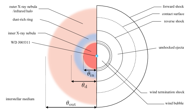
Figure 1: Schematic picture of the observed multi-wavelength morphology of IRAS 00500+6713 (left) and our dynamical model (right). A dusty infrared ring is sandwiched by the inner and outer X-ray nebulae. We assume that the inner X-ray nebula corresponds to the wind termination shock while the outer X-ray nebula to the shocked interface between the ejecta of SN 1181 and the interstellar matter, and the dust ring corresponds to the unshocked SN ejecta.

If indeed WD J005311 is a remnant of a double degenerate WD merger, the surrounding IRAS 00500+6713 nebula should hold the information on the merger dynamics and the post-merger evolution of the remnant. In fact, multi-wavelength observations of IRAS 00500+6713 have revealed its complicated morphology (see left part of Figure 1). The infrared image taken by the Wide-field Infrared Survey Explorer (WISE) shows a dust-rich ring with an angular size of $\theta_{\mathrm{d}}\sim 1\,\mathrm{arcmin}$ surrounded by a diffuse infrared halo extending to $\theta_{\mathrm{out}}\sim 139~{}\mathrm{arcsec}$ (Gvaramadze et al., 2019). Ritter et al. (2021) conducted a long-slit spectroscopic observation with OSIRIS on board the Gran Telescopio CANARIAS, and measured the expansion velocity of a layer surrounding the dust-rich ring at $\theta_{\mathrm{SII}}\sim 90\,\mathrm{arcsec}$ as $v_{\mathrm{SII}}\sim 1,100\,\mathrm{km\,s^{-1}}$ from the Doppler broadening of the [SII] line. Given $\theta_{\mathrm{SII}}$, $v_{\mathrm{SII}}$, and the distance to the source $d=2.3\,\mathrm{kpc}$ (Bailer-Jones et al., 2021), the age of IRAS 00500+6713 can be estimated to be $\sim 1,000$ yr. On the other hand, the observation with XMN-Newton identified the X-ray counterpart of IRAS 00500+6713, consisting of the inner nebula enveloped within the dust-rich ring and the outer nebula whose angular size is comparable to the infrared halo (Oskinova et al., 2020). The X-ray spectra indicate that both the inner and outer nebulae are also enriched with carbon burning ashes.

The outer X-ray nebula likely corresponds to the shocked interface between the interstellar matter (ISM) and an expanding matter ejected at the merger of the progenitor binary. From the angular size $\theta_{\mathrm{out}}$ and the emission measure of the outer X-ray nebula $\mathrm{EM}_{\mathrm{out}}$, Oskinova et al. (2020) estimated the ejecta mass as $M_{\mathrm{ej}}\sim 0.1~{}M_{\odot}$. Assuming that the bulk of the nebula is expanding with a velocity comparable with the dust-rich ring, i.e., $\sim 1,000\,\mathrm{km\,s^{-1}}$, the kinetic energy is estimated to be $E_{\mathrm{ej}}\sim 10^{48}\,\mathrm{erg}$. Such properties are compatible to so-called Type Iax supernovae (SNe Iax; Foley et al. 2013), which can be accompanied by the merger of carbon-oxygen and/or oxygen-neon WDs (see e.g., Kashyap et al., 2018). Interestingly, Ritter et al. (2021) and Lykou et al. (2022) pointed out that the sky location and the timing of the hypothesized merger are in accord with the ancient records on a historical Galactic SN, SN 1181. The documented apparent magnitude of SN 1181 is also consistent with SNe Iax, although the uncertainties are large Schaefer (2023).

The origin of the inner X-ray nebula is uncertain; the XMM image was reported to be consistent with a point source (Oskinova et al., 2020). Given that the intense wind with $v_{\mathrm{w}}=15,000\,\mathrm{km\,s^{-1}}$ is blowing toward the infrared halo expanding at a slower velocity $v_{\mathrm{SII}}\sim 1,100\,\mathrm{km\,s^{-1}}$, the wind termination shock would be the most likely possibility. Recently, Fesen et al. (2023) reported radially aligned filaments distributing in the dust-rich ring and the infrared halo, which can be due to the energy injection from the wind termination shock. As such, the intense wind can have significant impacts on the structure of IRAS 00500+6713 and accordingly on the values of the physical parameters estimated from the observed morphology. In addition, the history of the wind mass loss is directly connected to the time evolution and the fate of the merger product WD. Thus, it is crucial to construct a dynamical model that cohesively contains the wind, the SN ejecta, the ISM, and intervening multiple shocks (see right part of Figure 1).

In this paper, we first analyze the X-ray data on IRAS 00500+6713 obtained with XMM-Newton and Chandra to determine the angular size, emission measure, and metal abundance of the X-ray nebulae, taking into account the possible non-collisional ionization equilibrium (non-CIE) effects (Sec. 2). In particular, we newly obtain a constraint on the angular size of the inner X-ray nebula from the Chandra data. Next, we construct a dynamical model based on the hypothesis that IRAS 00500+6713 is the remnant of SN 1181 (Sec. 3). We consistently solve the dynamics of the inner and outer X-ray nebulae, allowing that the currently observed wind started to blow a finite time after SN 1181. We use the dynamical model to constrain the relevant physical parameters of the system, i.e., the SN explosion energy, the SN ejecta mass, the timing of the launch of the wind, from the currently observed multi-wavelength morphology. We discuss implications of the results of our dynamical model in Sec. 4.

2 X-ray data analysis

2.1 Observations and data reduction

IRAS 00500+6713 was observed with XMM-Newton in 2019 and 2021, and Chandra in 2021. We use the data obtained with the CCDs onboard both observatories, XMM EPIC (MOS1, MOS2, and pn; Turner et al. 2001; Strüder et al. 2001; Jansen et al. 2001) and Chandra ACIS (Garmire, 1997) for the imaging analysis. For the spectroscopy, we simultaneously use imaging spectroscopic data obtained with XMM EPIC and grating data obtained with XMM RGS (den Herder et al., 2001). Table 1 lists the observation logs. We use the XMM Science Analysis Software (SAS; v19.1.0; Gabriel et al. 2004) package, which also includes the Extended Source Analysis Software (ESAS; Snowden et al. 2004). We process the EPIC data with the SAS tasks pn-filter, epchain, emchain, and mos-filter. The RGS data are processed using the standard pipeline tool rgsproc in the SAS package. We exclude one observation (OBSID: 0872590301) because it shows high count rates over the whole field of view and is affected by background flares. The total effective exposures for the EPIC and RGS are $\approx 80$ ks and $\approx 110$ ks, respectively. The observation logs of Chandra are summerized in Table 2. We process the data with the CIAO (v4.15; Fruscione et al. 2006) tool chandra_repro. The total effective exposure is $\approx 144$ ks.

In the data analysis, we use the HEASoft (v6.20; HEASARC 2014), XSPEC (v12.9.1; Arnaud 1996), and AtomDB 3.0.9. The cstat (Cash, 1979) and wstat impremented in XSPEC are used in our spectral studies. In this section, uncertainties in the text, figures, and tables indicate 1$\sigma$ confidence intervals. The upper limits in this section are at a 95% confidence level.

Table 1: XMM observation logs of IRAS 00500+6713

OBSID	Start date	Exposure (ks)
0841640101	2019 Jul 8	14.2	19.5
0841640201	2019 Jul 24	13.4	16.7
0872590101	2021 Jan 8	6.8	11.8
0872590201	2021 Jan 10	10.9	12.9
0872590301	2021 Jan 14	4.0	7.9
0872590401	2021 Jan 16	7.7	17.2
0872590501	2021 Jan 20	10.4	12.7
0872590601	2021 Jan 18	12.2	14.6

Table 2: Chandra observation logs of IRAS 00500+6713

OBSID	Start date	Exposure (ks)
23419	2021 May 12	27.7
24342	2021 May 17	14.8
24343	2021 May 14	27.7
24344	2021 Oct 21	38.0
24345	2021 Dec 15	20.8
25045	2021 May 17	14.8

2.2 Analysis and results

2.2.1 Spatial distributions

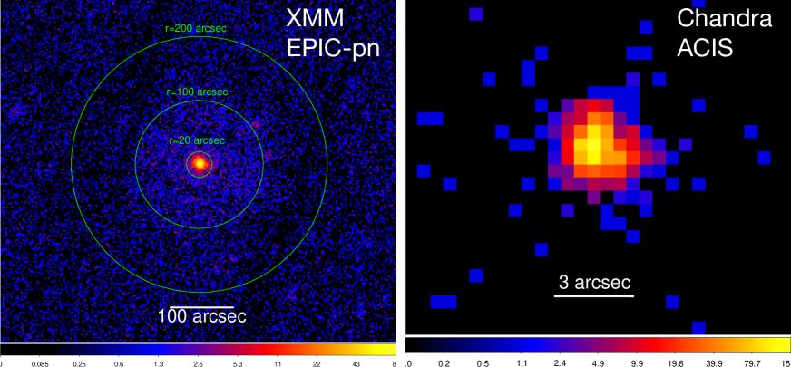
Figure 2: 0.5–5.0 keV images of IRAS 00500+6713 obtained with XMM EPIC-pn (left) and Chandra ACIS (right). For the XMM image, all the observations but one with OBSID 0872590301 are merged. All the observations are used to make the Chandra image. In the left panel, circles with radii of 20, 100, and 200 arcsec are overlaid in green. The former two correspond to the approximate spatial extents of the central and diffuse sources. The images are shown on a logarithmic scale.

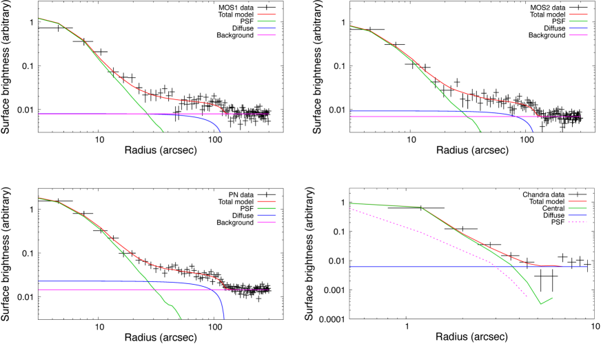
Figure 3: Radial flux profiles of IRAS 00500+6713 obtained with XMM MOS1, MOS2, pn, and Chandra ACIS. The XMM data are extracted from one observation in 2019 (OBSID: 0841640101). All the observations are merged for the Chandra data. The energy range for extraction is 0.5–5.0 keV. The solid lines represent the best-fit model components.

Figure 2 shows 0.5–5.0 keV X-ray images obtained with XMM EPIC-pn and Chandra ACIS. One can see a central source and faint diffuse emission around it. The central source is found to be slightly extended with the spatial resolution of Chandra ($\approx 0\farcs 5$). In order to evaluate the spatial distribution of the source, we extract radial profiles around the central source. The central position for extraction is set to (R.A., Decl.$)_{2000}=(13\fdg 2967,\,67\fdg 5007)$ by referring to the SIMBAD catalog. We take into account spatially-dependent exposures, bad pixels, and gaps between the CCDs. For the XMM EPIC CCDs, we obtain radial flux profiles for each instrument for each observation. For Chandra ACIS, we merge all the observations and extract radial profiles considering almost the same pointing directions and observation dates close to each other. In Figure 3, we show flux profiles extracted from one XMM observation in 2019 (OBSID: 0841640101) and the merged Chandra data.

We compare the observed distributions with a phenomenological model. The instrumental point spread functions (PSFs), i.e., the radial profiles of an ideal point source on the CCDs, are calculated for the source position with the SAS tool psfgen and CIAO tool simulate_psf. We assume a simple emission model for the central and diffuse sources: a sphere with a uniform and isotropic emissivity over the whole volume. The model for the radial flux profile ($F(r)$, where $r$ is the radius) is described as

$$F(r)=P(r,\theta_{\rm in})+D(r,\theta_{\rm out})+B,$$ (1)

with $P(r,\theta_{\rm in})$, $D(r,\theta_{\rm out})$, and $B$ being the fluxes of the central source, diffuse source, and background (assumed to be uniform), respectively. The parameters $\theta_{\rm in}$ and $\theta_{\rm out}$ indicate the spatial extents of the central and diffuse sources, respectively. $P(r,\theta_{\rm in})$ and $D(r,\theta_{\rm out})$ are spherical emission convolved with the instrumental PSFs. We mainly focus on evaluation of $\theta_{\rm in}$ and $\theta_{\rm out}$.

We use the MCMC (Markov Chain Monte Carlo) algorithm to determine the best-fit model parameters and their confidence ranges. To perform a precise evaluation, the profiles extracted from all the instruments in all the observations (21 in total) are modeled simultaneously via linked $\theta_{\rm in}$ and $\theta_{\rm out}$ for the XMM data. The normalizations of $P(r,\theta_{\rm in})$ and $D(r,\theta_{\rm out})$, and $B$ for individual instruments are treated as free parameters. Radial ranges of 0–300 and 0–10 arcsec are used for the modeling of the XMM and Chandra data, respectively. As a result, we obtain $\theta_{\rm in}<1.5$ arcsec and $\theta_{\rm out}=131^{+2}_{-2-2}$ arcsec with the XMM data. The spatial extent of the diffuse source is similar to that in infrared (Gvaramadze et al., 2019). On the other hand, we are able to constrain the radius as $\theta_{\rm in}=1.52^{+0.08}_{-0.08-0.67}$ arcsec with the Chandra flux profile. The best-fit models are overlaid in Figure 3. We also search for a possible time variation of the spatial distributions by separately modeling the XMM flux profiles in 2019 and 2021. We find results consistent with each other, $\theta_{\rm in}<1.5$ arcsec and $\theta_{\rm out}=132\pm 2$ arcsec in 2019 and $\theta_{\rm in}<1.5$ arcsec and $\theta_{\rm out}=129\pm 3$ arcsec in 2021.

The background rates $B$ determined from the XMM data, e.g., $\approx 0.0023$ counts s^-1 arcmin^-2 (0.5–5.0 keV) for MOS1 in 2021, are consistent with or slightly higher than the pure particle background rate (Kuntz & Snowden, 2008). This is reasonable considering the contribution of sky background. The diffuse plus background flux $D(r,\theta_{\rm out})+B$ for the Chandra data are also consistent with the sum of the diffuse flux determined from the XMM data and the particle background rate (Bartalucci et al., 2014; Suzuki et al., 2021).

2.2.2 Spectral properties of the thermal plasmas

We here extract energy spectra and estimate the temperatures, metal abundances, ionization time scale, and emission measures of the central and diffuse sources. We use the XMM data, which have much greater statistics than the Chandra data. Spectral extraction regions for the EPIC data are selected based on the imaging analysis results (Figure 3) and are shown in Figure 2. A circle with a 20 arcsec radius is used for the central source, and an annulus with inner and outer radii of 30 and 100 arcsec, respectively, is assumed for the diffuse source. As the background, we use the diffuse source and an annulus region with inner and outer radii of 100 and 200 arcsec, respectively. The central position for extraction is the same as that used for the extraction of the radial profiles. Since the RGS spectrum has much poorer statistics, we only use it as a consistency check for the spectral analysis of the bright central source. We merge all the spectra in each year and for each instrument: the 1st- and 2nd-order spectra are also combined for the RGS data. The spatial variation of the detector background is negligible considering the on-axis position and sizes of our analysis regions, and moderate statistics (Kuntz & Snowden, 2008).

As the spectral model, we consider thermal plasmas in two different assumptions of metalicity by referring to Oskinova et al. (2020): near solar and pure metal. Under each assumption, we adopt a minimal model configuration that explains the data sufficiently well. An absorbed ionizing plasma model (${\tt tbabs}\times{\tt nei}$) is assumed for both cases. In the case of the near-solar plasma, the hydrogen column density ($N_{\rm H}$), electron temperature ($kT_{\rm e}$), ionization timescale ($\tau$), emission measure, and abundances of O, Ne, Mg, and Fe ($=$Ni) are treated as free parameters. The other metal abundances are fixed to solar. In the pure-metal case, the same model but without H, He, N, Ar, and Ca is used. The free parameters are the same as above but the abundance of O is fixed to solar and Ne is set free. The spectra obtained with all the instruments in 2019 and 2021 (six in total) are modeled simultaneously. We use the energy ranges of 0.5–5.0 keV and 0.5–2.0 keV for the spectral fit of the central and diffuse sources, respectively, considering their statistics.

The spectra and best-fit models are presented in Figure 4. Table 3 shows the best-fit parameters. Both models explain well both central and diffuse sources. Oskinova et al. (2020) applied a two-temperature, collisional-ionization-equilibrium thermal plasma model to these sources. Compared to their results, the electron temperatures we obtain here lie between their higher and lower temperatures. The absorption column densities are found to be similar. It will be meaningless to compare the metal abundances because of the differences in the model assumptions. We also search for possible spectral changes as a function of time but find no such evidence.

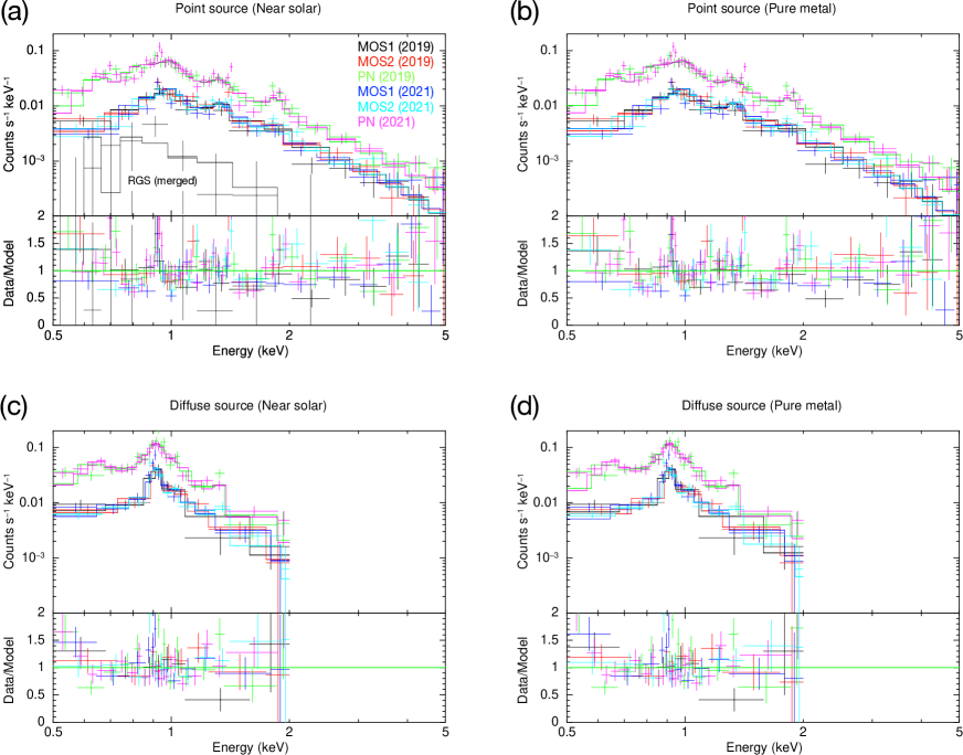
Figure 4: Energy spectra extracted from the central point-like source (panels (a) and (b)) and surrounding diffuse source (panels (c) and (d)). Multiple observations in each year are merged. The solid lines show the best-fit models in the two cases (near solar and pure metal). The upper and lower panels present the spectra and data-to-model ratios, respectively. The background spectra are subtracted from all the data. The XMM RGS spectrum, which is used for a consistency check, is presented in the panel (a).

Table 3: Best-fit spectral parameters for the point-like and diffuse sources

		$N_{\rm H}$ ($10^{22}\,{\rm cm}^{-2}$)	$kT_{\rm e}$ (keV)	$\tau$	O	Ne	Mg	Fe ($=$Ni)	$\mathrm{EM}$	C-stat/d.o.f.
Point source	Near solar	0.78$\pm$0.05	1.30$\pm$0.08	7.9$\pm$1.3	31$\pm$8	1 (fixed)	0.68$\pm$0.25	2.81$\pm$0.63	(1.8$\pm$0.4)$\times 10^{2}$	4406/5409
	Pure metal	0.75$\pm$0.05	1.21$\pm$0.06	9.5$\pm$1.4	37$\pm$9	1 (fixed)	0.70$\pm$0.25	2.62$\pm$0.62	6.3$\pm$1.1	4405/5409
Diffuse source	Near solar	0.51$\pm$0.05	0.65$\pm$0.02	$3.9\pm 0.4$	1 (fixed)	2.83$\pm$0.44	1.01$\pm$0.27	0.06$\pm$0.04	(3.7$\pm$1.0)$\times 10^{2}$	2075/1809
	Pure metal	0.51$\pm$0.05	0.30$\pm$0.03	$>53$	1 (fixed)	1.78$\pm$0.27	0.83$\pm$0.24	0.06$\pm$0.04	3.6$\pm$0.8	2061/1809

Table 4: Parameters in our dynamical model for IRAS 00500+671.

	observed parameter		reference
distance	$d$ [kpc]	$2.3^{+0.1}_{-0.1}$	Gaia Collaboration et al. (2021)
wind mass loss rate	$\dot{M}_{\mathrm{w}}$ [$M_{\odot}\,\mathrm{yr^{-1}}$]	$(7.5\mbox{--}40)\times 10^{-7}$	Lykou et al. (2022)
wind mechanical luminosity	$L_{\mathrm{w}}$ [${\rm erg\,s^{-1}}$]	$(0.53\mbox{--}2.8)\times 10^{38}$	Lykou et al. (2022)
angular size	$\theta_{\rm in}$ [arcsec]	$0.77-1.6$	This work
	$\theta_{\rm out}$ [arcsec]	$129^{+3}_{-3}$	This work
	$\theta_{\rm d}$ [arcsec]	$60^{+12}_{-12}$	Gvaramadze et al. (2019)
expansion velocity	$v_{\mathrm{SII}}$ [${\rm km\,s^{-1}}$]	$1100^{+100}_{-100}$	Ritter et al. (2021)
emission measure	${\rm EM}_{\rm in}$ [$10^{52}\,{\rm cm^{-3}}$]	180$\pm$40 (near-solar)	This work
		6.3$\pm$1.1 (pure metal)	This work
	${\rm EM}_{\rm out}$ [$10^{52}\,{\rm cm^{-3}}$]	370$\pm$100 (near-solar)	This work
		3.6$\pm$0.8 (pure metal)	This work
	model parameter
power-law index of the SN ejecta density profile	$n$	6 (fixed)
	$\delta$	1.5 (fixed)
number density of ISM	$n_{\mathrm{ISM}}$ [cm-3]	$0.097\mbox{--}0.13$
explosion energy	$E_{\mathrm{ej}}$ [$10^{48}$ erg]	$0.77\mbox{--}1.1$
ejecta mass	$M_{\mathrm{ej}}$ [$M_{\odot}$]	$0.18\mbox{--}0.53$
wind launching time	$t_{\mathrm{w}}$ [yr]	$810\mbox{--}828$

3 Dynamical Model

In the previous section, we have determined the amounts and spatial extents of the X-ray emitting plasma in the inner and outer nebulae of IRAS 00500+6713, i.e., the emission measures ($\mathrm{EM}_{\mathrm{in}}$ and $\mathrm{EM}_{\mathrm{out}}$) and the angular sizes ($\theta_{\mathrm{in}}$ and $\theta_{\mathrm{out}}$). Note that the obtained values of EMs are different from those shown in Oskinova et al. (2020). This is mainly because the assumed distance to the source is different; we use the updated Gaia eDR3 value $d_{\mathrm{eDR3}}=2.3\pm 0.1\,\mathrm{kpc}$ (Gaia Collaboration et al., 2021) while Oskinova et al. (2020) used the Gaia DR2 value $d_{\mathrm{DR2}}=3.1\,\mathrm{kpc}$.

Here we construct a dynamical model of IRAS 00500+6713 for interpreting the currently observed X-ray properties. The schematic picture of the overall structure is shown in Figure 1. We assume that the inner shocked region is produced by the interaction between the ejecta of SN 1181, set to be launched at $t=0$, and the wind from the central WD that started blowing at $t=t_{\mathrm{w}}$. On the other hand, the outer shocked region is produced by the interaction between the SN ejecta and the surrounding ISM. We follow the dynamical evolution of the inner and outer X-ray nebulae from the onset of the SN explosion ($t=0$) through $t=845\,\mathrm{yr}$ ($t=840$ yr corresponds to A.D. 2021) to determine the characteristic quantities of the system, i.e., the explosion energy $E_{\mathrm{ej}}$ and the ejecta mass $M_{\mathrm{ej}}$ of SN 1181 and the timing $t_{\mathrm{w}}$ of the launch of the wind that reproduce the X-ray properties.

We note that other than EMs and $\theta$s, there are observed properties of IRAS 00500+6713 that might be useful to constrain the model. For example, the electron temperatures $kT_{\mathrm{e}}$ and the ionization timescales $\tau$ have been estimated. In addition, the previous mid-infrared observations determined the angular size $\theta_{\mathrm{d}}$ of the dust-rich ring and the expansion velocity $v_{\mathrm{SII}}$ of the infrared halo (Gvaramadze et al., 2019; Ritter et al., 2021). We mainly use these pieces of information to check which models fit the EMs and $\theta$s of the X-ray nebulae and satisfy conditions required from these observations. The ranges of physical parameters that best reproduce the X-ray observations are listed in Table 4.

3.1 Density profiles

In order to calculate the evolution of this system, the density profile of each region should be given. The density profile of the SN ejecta is often described by a double power law (Chevalier & Soker, 1989; Matzner & McKee, 1999; Moriya et al., 2013);

$$\rho_{\mathrm{ej}}=\rho_{\mathrm{ej,br}}\times\begin{cases}(r/r_{\mathrm{br}})^{-\delta}&r<r_{\mathrm{br}}\\ (r/r_{\mathrm{br}})^{-n}&r>r_{\mathrm{br}},\end{cases}$$ (2)

where

$$\rho_{\mathrm{ej,br}}=t^{-3}(r_{\mathrm{br}}/tg)^{-n},$$ (3)

$$r_{\rm br}=\left[\frac{2(5-\delta)(n-5)E_{\rm ej}}{(3-\delta)(n-3)M_{\rm ej}}\right]^{\frac{1}{2}}t,$$ (4)

$$g^{n}=\frac{1}{4\pi(n-\delta)}\frac{\left[2(5-\delta)(n-5)E_{\rm ej}\right]^{\frac{n-3}{2}}}{\left[(3-\delta)(n-3)M_{\rm ej}\right]^{\frac{n-5}{2}}}.$$ (5)

$E_{\mathrm{ej}}$ and $M_{\mathrm{ej}}$ are the explosion energy and the ejecta mass of the SN, respectively. In order to have a finite total mass and energy, $n>5$ and $\delta<3$ are required (Chevalier, 1982). We assume that the SN ejecta is surrounded by ISM with a constant mass density of

$$\rho_{\rm ISM}=\mu_{\rm ISM}m_{\rm u}n_{\rm ISM}$$ (6)

where $\mu_{\rm ISM}=0.615$ is the mean molecular weight assuming the solar abundance, $m_{\rm u}$ is the atomic mass unit, and $n_{\rm ISM}$ is the number density of the ISM. On the other hand, WD J005311 resides inside the SN ejecta and blows an intense wind with a mass loss rate of $\dot{M}_{\mathrm{w}}=(7.5\mbox{--}40)\times 10^{-7}~{}M_{\odot}\,\mathrm{yr}^{-1}$ and velocity of $v_{\mathrm{w}}=15,000~{}\mathrm{km\,s^{-1}}$ (Lykou et al., 2022). Accordingly, the mechanical luminosity of the wind can be estimated as $L_{\mathrm{w}}=\dot{M}_{\rm w}v_{\rm wind}^{2}/2=(0.53\mbox{--}2.8)\times 10^{38}\,\mathrm{erg\,s^{-1}}$. We assume that the currently observed wind from WD J005311started blowing at $t=t_{\mathrm{w}}$ with a constant mass loss rate after the SN explosion. The density profile in the wind region is described as

$$\rho_{\mathrm{w}}=\frac{\dot{M}_{\mathrm{w}}}{4\pi r^{2}v_{\mathrm{w}}}.$$ (7)

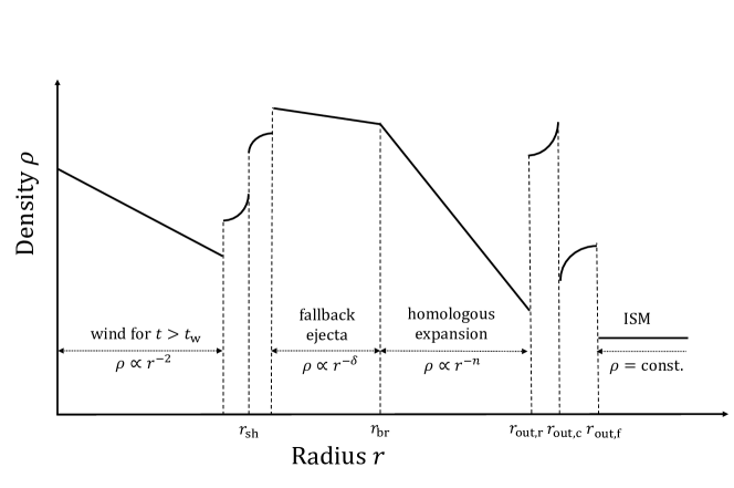
Figure 5: A schematic picture of the radial density profile of IRAS 00500+6713.

The radial density profile is shown schematically in Figure 5. While the SN ejecta expands in the ISM, the wind catches up and collides with the SN ejecta. Two shocked regions form; one between the wind and the SN ejecta, and the other between the SN ejecta and the ISM. The inner and outer X-ray nebulae are powered by the heated material in these two shocked regions . In between the two shocked regions, there can be an unshocked layer. In our view, both the dusty infrared ring detected in the WISE image and the [SII] line emission region detected by OSIRIS correspond to this unshocked layer; when the shocks sweep through this layer, dust grains are expected to be destroyed.

3.2 Outer X-ray nebula

Let us first consider the outer X-ray nebula. For homologously expanding SN ejecta sweeping a uniform ISM described in Sec. 3.1, we can employ the self-similar solution of Chevalier (1982) to describe the evolution of the shocked region. The actual values of the exponents of the density profile should depend on the progenitor system and the mechanism of the SN explosion. While the exponent in the range $7\lesssim n\lesssim 10$ has been inferred from simulations for Type Ia SNe (e.g., Colgate & McKee, 1969; Kasen, 2010), the exponent may become smaller for weaker explosions such as Type Iax SNe. Actually, simulations of the mass eruption from a massive star before core-collapse have found a profile of $n\sim 6$ (e.g., Kuriyama & Shigeyama, 2020; Tsuna et al., 2020). Given that, we consider a range of $6\leq n\leq 10$ and set $n=6$ as the fiducial value. In this case, the radii of the forward shock $r_{\mathrm{out,f}}$, the contact discontinuity $r_{\mathrm{out,c}}$, and the reverse shock $r_{\mathrm{out,r}}$ all evolve with the same power-law in time;

$$r_{\mathrm{out,}i}=\left(A_{i}g/\rho_{\rm ISM}^{1/6}\right)t^{1/2}\ (i={\rm f},\ {\rm c},\ {\rm r}).$$ (8)

The proportionality factors $A_{i}$ for these radii, as well as the density, pressure, and velocity profiles inside both the shocked ejecta and the shocked ISM, are obtained for a given set of parameters ($E_{\mathrm{ej}},M_{\mathrm{ej}},n_{\mathrm{ISM}}$) . We assume an adiabatic index of $\gamma=5/3$.

3.2.1 Angular size

As we have shown in Sec. 2, the angular size of the outer X-ray nebula is $\theta_{\rm out}=131\pm 2~{}$arcsec based on the XMM-Newton observation in 2021 January. In our model, this corresponds to the forward shock radius $r_{\mathrm{out,f}}$ at $t=840\,\mathrm{yr}$:

$$r_{\rm out,f}=1.44_{-0.10}^{+0.09}~{}\mathrm{pc}.$$ (9)

Note that the estimated error of $r_{\rm out,f}$ is smaller than errors of the other parameters, thus we neglect the error hereafter. Applying this condition to the self-similar solution described above, we obtain a condition

$$\left(\frac{E_{\rm ej}}{10^{48}\,\mathrm{erg}}\right)^{-1/2}\left(\frac{M_{\rm ej}}{0.5~{}M_{\odot}}\right)^{1/6}\left(\frac{\mu_{\rm ISM}n_{\rm ISM}}{0.1~{}\mathrm{cm}^{-3}}\right)^{1/3}=0.86.$$ (10)

3.2.2 Emission measure

The emission measure of the outer X-ray nebula can be described as

$$\mathrm{EM}_{\mathrm{out}}=n_{\rm e}n_{\rm ion}V=\frac{4\pi}{m_{\rm u}^{2}}\left(\frac{1}{\mu_{\rm r}^{2}}\int_{r_{\rm out,r}}^{r_{\rm out,c}}r^{2}\rho(r)^{2}dr+\frac{1}{\mu_{\rm f}^{2}}\int_{r_{\rm out,c}}^{r_{\rm out,f}}r^{2}\rho(r)^{2}dr\right).$$ (11)

The first term in the right-hand side of Eq. (11) represents the contribution from the reverse shock or the shocked ejecta; $\mu_{\mathrm{r}}$ is the mean molecular weight and $\rho(r)$ is the density. The second term represents the contribution from the forward shock, or the shocked ISM, where $\mu_{\mathrm{f}}$ is the mean molecular weight. Using the shock structure obtained from the self-similar solution, the integrals of Eq. (11) can be calculated as

$$\int_{r_{\rm out,c}}^{r_{\rm out,f}}r^{2}\rho^{2}dr=2.15\times 10^{6}\,\mathrm{g}^{2}\mathrm{cm}^{-3}\left(\frac{n_{\rm ISM}}{0.1\,\mathrm{cm}^{-3}}\right)^{2},$$ (12)

$$\int_{r_{\rm out,r}}^{r_{\rm out,c}}r^{2}\rho^{2}dr=8.96\times 10^{6}\,\mathrm{g}^{2}\mathrm{cm}^{-3}\left(\frac{n_{\rm ISM}}{0.1\,\mathrm{cm}^{-3}}\right)^{2}.$$ (13)

Note that they do not depend on either $E_{\mathrm{ej}}$ or $M_{\mathrm{ej}}$ for a given $r_{\rm out,f}$. As for the mean molecular weight in the shocked ejecta, we set it to be consistent with the pure metal model of the X-ray analysis in Sec. 2:

$$\mu_{\rm r}^{2}=\mu_{\rm e,r}\mu_{\rm ion,r},$$ (14)

where

$$\frac{1}{\mu_{\rm e,r}}=\sum_{i}\frac{\langle n\rangle_{i}X_{i}}{A_{i}}=0.466,$$ (15)

$$\frac{1}{\mu_{\rm ion,r}}=\sum_{i}\frac{X_{i}}{A_{i}}=0.060.$$ (16)

Here, $X_{i}$ denotes the mass fraction of element $i$, $A_{i}$ its mass number, and $\langle n\rangle_{i}$ is the average number of free electrons originating from element $i$. The number of free electrons is obtained from AtomDB 3.0.9 (Foster et al., 2012) using the abundance ratios and the ionization degree for each element. We have used $kT_{\rm e}$and $\tau$ obtained from our X-ray analysis to estimate the degree of ionization. On the other hand, the mean molecular weight in the shocked ISM is set to that of the near-solar composition:

$$\mu_{\rm f}^{2}=\mu_{\rm e,f}\mu_{\rm ion,f},$$ (17)

where

$$\frac{1}{\mu_{\rm e,f}}\sim\frac{1}{\mu_{\rm e,solar}}\approx X\times\frac{1}{1}+Y\times\frac{2}{4}=0.85,$$ (18)

$$\frac{1}{\mu_{\rm ion,f}}\sim\frac{1}{\mu_{\rm ion,solar}}\approx X\times\frac{1}{1}+Y\times\frac{1}{4}=0.775.$$ (19)

Here $X$ and $Y$ are the mass fractions of hydrogen and helium, respectively.

The EM obtained from the X-ray analysis assumes a one-zone uniform shocked gas, while our EM model is a two-zone with different abundances. Though this makes a straightforward comparison difficult, the abundance of the mixture of the two regions is expected to be close to the ISM composition in the above self-similar solution because the mass ratio of the shocked ejecta to the shocked ISM is determined to be $0.28$. Thus, we compare the calculated EM (Eq. 11) with the value obtained by the X-ray analysis assuming the near-solar abundance. By substituting Eqs. (12-19) into Eq. (11), we can determine the ISM number density as

$${n_{\rm ISM}}=0.11~{}\mathrm{cm}^{-3}\left(\frac{\mathrm{EM}_{\rm out}}{3.7\times 10^{54}~{}\mathrm{cm}^{-3}}\right)^{1/2}.$$ (20)

Substituting this into Eq. (10), we obtain a condition

$$\left(\frac{E_{\rm ej}}{10^{48}\,\mathrm{erg}}\right)^{-1/2}\left(\frac{M_{\rm ej}}{0.5~{}M_{\odot}}\right)^{1/6}=0.97\left(\frac{\mathrm{EM}_{\rm out}}{3.7\times 10^{54}~{}\mathrm{cm}^{-3}}\right)^{-1/6}.$$ (21)

Figure 6 shows the obtained relation between $E_{\mathrm{ej}}$ and $M_{\mathrm{ej}}$. Given that IRAS 00500+6713 hosts a WD remnant, the ejecta mass would not be larger than $M_{\mathrm{ej}}\lesssim 1\,M_{\odot}$. In this case, the explosion energy is constrained to be $E_{\mathrm{ej}}\lesssim 10^{48}\,\mathrm{erg}$ only from the outer X-ray nebula. These results are broadly consistent with the previous work (Oskinova et al., 2020).

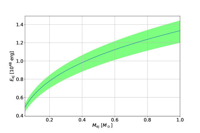
Figure 6: The arrowed range of the explosion energy $E_{\mathrm{ej}}$ and the ejecta mass $M_{\mathrm{ej}}$ of SN 1181 obtained from our modeling of the outer X-ray nebula of IRAS 00500+6713 (Eq. 21). The blue line and the green shaded region correspond to the best-fit value and 2$\sigma$ uncertainties of the emission measure EM_out obtained in Sec. 2.

3.3 Inner X-ray nebula

Next, we consider the inner X-ray nebula. We calculate the position of the contact surface between the shocked wind and shocked ejecta using the thin shell approximation (e.g., Chevalier & Fransson, 1992). The mass, momentum, and energy conservations of the shell can be described as

$$\frac{d}{dt}M_{\rm sh,in}=\dot{M}_{\rm w}+4\pi r_{\rm sh}^{2}\rho_{\rm ej}(r_{\rm sh})\left(v_{\rm sh}+\sqrt{\frac{2GM_{*}}{r_{\rm sh}}}\right).$$ (22)

$$M_{\mathrm{sh,in}}\frac{dv_{\mathrm{sh}}}{dt}=4\pi r_{\mathrm{sh}}^{2}\left[p_{\rm sh}-\rho_{\mathrm{ej}}(r_{\mathrm{sh}})\left(v_{\mathrm{sh}}+\sqrt{\frac{2GM_{*}}{r_{\rm sh}}}\right)^{2}\right]-\frac{GM_{\mathrm{sh,in}}M_{*}}{r_{\mathrm{sh}}^{2}},$$ (23)

$$\frac{d}{dt}\left[\frac{4\pi r_{\mathrm{sh}}^{3}}{3}\frac{p_{\rm sh}}{\gamma-1}\right]=L_{\mathrm{w}}-p_{\rm sh}\times 4\pi r_{\mathrm{sh}}^{2}v_{\mathrm{sh}},$$ (24)

respectively. Here $M_{\mathrm{sh,in}}$, $r_{\mathrm{sh}}$, $v_{\mathrm{sh}}$ are the mass, radius, and velocity of the shocked shell, respectively. The mass of the central star is denoted by $M_{*}$, $p_{\rm sh}$ is the pressure in the wind bubble, $\rho_{\mathrm{ej}}$ is the unshocked ejecta density, and $v_{\mathrm{ej}}$ is the velocity. In Eqs. (22) and (24), we assume that the tail part of the SN ejecta is falling back toward the central WD with a velocity of $-\sqrt{2GM_{*}/r_{\mathrm{sh}}}$. This can be justified given that the inferred explosion energy from the outer X-ray nebula, $E_{\mathrm{ej}}\sim 10^{48}\,\mathrm{erg}$ (see Figure 6), is much smaller than the gravitational binding energy of the central WD, $GM_{*}^{2}/R_{*}\sim 10^{50}\,\mathrm{erg}$. The density at the forward shock front is estimated from Eq. (2) with fixing $\delta=1.5$, which is appropriate for a fallback tail (e.g., Tsuna et al., 2021b).

In order to follow the evolution of the inner nebula, we integrate Eqs. (22), (23), and (24) from $t=t_{\rm w}$ for a given set of ($t_{\rm w}$, $E_{\rm{ej}}$, $M_{\rm{ej}}$). After using the constraint from the outer X-ray nebula (Eq. 21), we have two independent parameters ($t_{\rm w}$, $M_{\rm{ej}}$). The initial conditions are given as $[v_{\rm sh,0},p_{\rm sh,0},M_{\rm sh,0}]=[-\sqrt{2GM_{*}/r_{\rm sh,0}},3(\gamma-1)L_{\rm w}/4\pi r_{\rm sh,0}^{2}v_{\mathrm{w}},\int_{R_{*}}^{r_{\rm sh,0}}4\pi r^{2}\rho_{\rm ej}(r)dr]$. We set the initial shell radius sufficiently small, $r_{\rm sh,0}=10^{10}\,\mathrm{cm}$ so that the initial conditions do not affect the evolution on a timescale of 100 yr. We investigate a range of wind mass loss rate $\dot{M}_{\mathrm{w}}=(7.5\mbox{--}40)\times 10^{-7}\,M_{\odot}\,\mathrm{yr}^{-1}$, inferred from the optical spectroscopic observations.

3.3.1 Angular size

As we show in Sec. 2, the angular size of the inner X-ray nebula is constrained as $0.77\,\mathrm{arcsec}<\theta_{\rm in}<1.6$ arcsec based on the Chandra observation in 2021. In our model, this corresponds to the thin shell radius, i.e. the radius of the wind termination shock $r_{\mathrm{sh}}$ at $t=840\,\mathrm{yr}$:

$$0.0087~{}\mathrm{pc}<r_{\rm sh}<0.018~{}\mathrm{pc}.$$ (25)

Figure 7 shows the time evolution of the inner nebula radius calculated for several parameter sets. One can see that $r_{\rm sh}$ at $t=840\,\mathrm{yr}$ becomes larger for a smaller $M_{\rm ej}$, a larger $\dot{M}_{\rm w}$, and/or smaller $t_{\mathrm{w}}$. This is simply because the wind keeps pushing the fallback ejecta since its beginning. Therefore, too small $M_{\rm ej}$ or too small $t_{\rm w}$ leads to a too-expanded shell, which is inconsistent with the Chandra observation. This can give a constraint on the parameter set $(\dot{M}_{\rm w},t_{\rm w},M_{\rm{ej}})$.

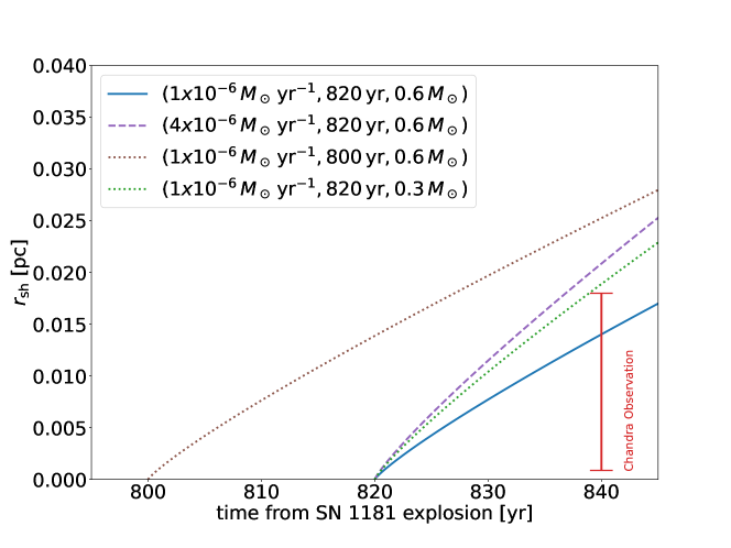
Figure 7: The time evolution of the radius of the inner X-ray nebula $r_{\mathrm{sh}}$ calculated for several parameter sets $(\dot{M}_{\rm w},t_{\rm w},M_{\rm{ej}})$ using our dynamical model. The red line indicates the value obtained by the Chandra observations.

3.3.2 Emission measure

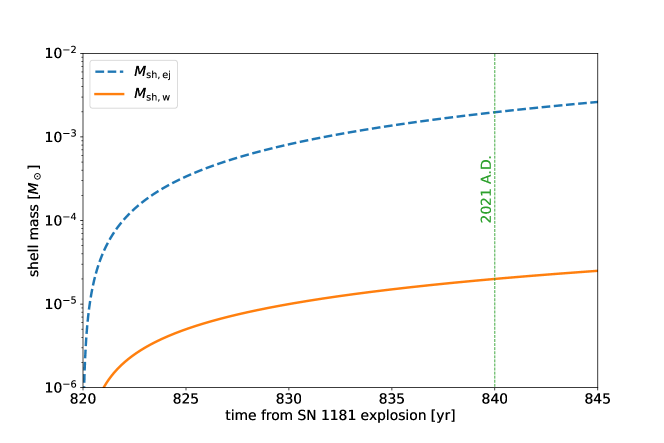
Figure 8: The time evolution of the mass in the shocked wind (orange solid line) and the shocked SN ejecta (blue dashed line) of the inner X-ray nebula, calculated for a parameter set $(\dot{M}_{\rm w},t_{\rm w},M_{\rm{ej}})=(1\times 10^{-6}~{}M_{\odot}\,\mathrm{yr}^{-1},820~{}\mathrm{yr},0.3~{}M_{\odot})$ using our dynamical model. The green dotted line indicates the year 2021 AD when the X-ray observations were done.

By modeling the expansion of the inner nebula, we can also estimate the total mass in the shocked region. Figure 8 shows the time evolution of the shocked mass for a case with $(\dot{M}_{\rm w},t_{\rm w},M_{\rm{ej}})=(1\times 10^{-6}~{}M_{\odot}\,\mathrm{yr}^{-1},820~{}\mathrm{yr},0.6~{}M_{\odot})$. The solid and dashed lines indicate the contribution from the shocked wind swept by the reverse shock and the shocked SN ejecta swept by the forward shock, respectively. One can see that the latter is 2-3 orders of magnitude larger than the former. Importantly, however, the shocked SN ejecta component will not contribute to the emission measure of the inner X-ray nebula; as we show in Appendix A, the electron temperature is kept below $3\mbox{--}4\,\mathrm{eV}$ in the shocked SN ejecta. Thus, we only consider the shocked wind as the source of the inner X-ray nebula. In this case, the emission measure of the inner nebula can be estimated as

$$\mathrm{EM}_{\rm in}=n_{\rm e}n_{\rm ion}V_{\rm sh,w}=\frac{M_{\rm sh,w}^{2}}{\mu_{\rm e}\mu_{\rm ion}m_{\rm u}^{2}V_{\rm sh,w}},$$ (26)

where $M_{\mathrm{sh,w}}=\dot{M}_{\mathrm{w}}(t-t_{\mathrm{w}})$ is the total mass of the shocked wind, and

$$V_{\mathrm{sh,w}}\approx\frac{4}{3}\pi\left(r_{\mathrm{sh}}^{3}-r_{\mathrm{in,r}}^{3}\right)=\frac{4}{3}\pi r_{\mathrm{sh}}^{3}\left[1-\left(\frac{2}{1+\gamma}\right)^{3}\right]$$ (27)

is the volume of the shocked wind region. Here we estimate the positions of the reverse shock fronts as

$$r_{\mathrm{in,r}}\approx(1-{\cal C})r_{\mathrm{sh}}=\frac{2}{1+\gamma}r_{\mathrm{sh}}.$$ (28)

With an approximation that the shock region is plane-parallel and adiabatic, the compression ratio is ${\cal C}=(\gamma-1)/(\gamma+1)=4$ for $\gamma=5/3$ in the strong shock limit. The mean molecular weights in the shocked wind region are calculated for pure metal abundance with ionization inferred from the X-ray spectroscopy in Sec. 2:

$$\frac{1}{\mu_{\rm e,metal}}=\sum_{i}\frac{\langle n\rangle_{i}X_{i}}{A_{i}}=0.49,$$ (29)

$$\frac{1}{\mu_{\rm ion,metal}}=\sum_{i}\frac{X_{i}}{A_{i}}\sim 0.062.$$ (30)

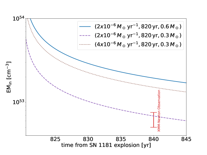
Figure 9: The time evolution of the emission measure of the inner X-ray nebula EM_in calculated for several parameter sets $(\dot{M}_{\rm w},t_{\rm w},M_{\rm{ej}})$ using our dynamical model. The red line indicates the value obtained by the XMM-Newton observations.

By comparing the calculated EM_in of the shocked wind (Eq. 26) with the observed value for the pure metal model (Tables 3 and 4), we can obtain an additional constraint on our model parameters:

$$5.0\times 10^{52}~{}\mathrm{cm}^{-3}<\mathrm{EM}_{\rm in}<7.6\times 10^{52}~{}\mathrm{cm}^{-3}$$ (31)

Figure 9 shows the time evolution of EM_in calculated for several parameter sets. As expected, a larger $\dot{M}_{\mathrm{w}}$ gives a larger shocked mass and thus a larger EM_in. In addition, a larger $M_{\mathrm{ej}}$ also gives a larger EM_in; this is because the inner nebula expansion becomes slower for a larger $M_{\mathrm{ej}}$ and thus the volume of the inner nebula $V_{\mathrm{sh,w}}$ becomes smaller (see Eq. 26).

3.4 Model parameter determination

Combining all the conditions shown in the previous subsections, we here determine the parameters of our dynamical model. First, we constrain the ISM density $n_{\rm ISM}$ (Eq. 20) and obtain a relation between $E_{\rm{ej}}$ and $M_{\rm{ej}}$ (Eq. 21) from the observed size and EM of the outer X-ray nebula. Then, we search sets of the residual parameters ($t_{\mathrm{w}}$, $M_{\mathrm{ej}}$) that can consistently explain the observed size and EM of the inner X-ray nebula. In doing so, we allow the wind mass loss rate $\dot{M}_{\mathrm{w}}$ to vary in the range inferred from the optical spectroscopy.

Figure 10: Constraints on the parameters of our dynamical model. The shaded region indicates the allowed range of the parameters with respect to the ejecta mass (lower horizontal axis) and the explosion energy (upper horizontal axis) of SN 1181, and the timing of the launch of the currently observed wind (vertical axis). The relation between the upper and lower horizontal axis is based on Eq. (21). The red dashed line indicates the timing of the XRT observation of IRAS 00500+6713.

Figure 10 shows the allowed range of the parameters with respect to the SN ejecta mass $M_{\mathrm{ej}}$ (lower horizontal axis), the SN explosion energy $E_{\mathrm{ej}}$ (upper horizontal axis), and the timing of the wind launch $\Delta t_{\mathrm{w}}=840~{}\mathrm{yr}-t_{\rm w}~{}[\mathrm{yr}]$ (vertical axis) consistent with the X-ray observations by XMM-Newton and Chandra. We find that the size constraint of the inner nebula is tight; in order to confine the wind termination shock as observed, it only allows a very recent launch of the wind and a sufficiently large ejecta mass. On the other hand, the combination of the emission measures of the inner and outer nebulae set an upper limit on the ejecta mass. In Figure 10, we also indicate the timing of a past X-ray observation by Swift XRT in 2012 A.D., which identified a comparably bright counterpart as the currently observed inner X-ray nebula (Evans et al., 2014; Lykou et al., 2022). We regard that this sets a lower limit for $\Delta t_{\mathrm{w}}$. In summary, we obtain the following constraints on the model parameters:

$$0.097~{}\mathrm{cm}^{-3}<n_{\mathrm{ISM}}<0.13~{}\mathrm{cm}^{-3},$$ (32)

$$0.77\times 10^{48}~{}\mathrm{erg}<E_{\rm ej}<1.1\times 10^{48}~{}\mathrm{erg},$$ (33)

$$0.18~{}M_{\odot}<M_{\rm ej}<0.53~{}M_{\odot},$$ (34)

and

$$12~{}\mathrm{yr}<\Delta t_{\rm w}<30~{}\mathrm{yr},$$ (35)

or

$$810~{}\mathrm{yr}<t_{\rm w}<828~{}\mathrm{yr},$$ (36)

3.5 Consistency check with other observations

The model parameters (Eqs. 32-36) are obtained by mainly fitting the angular sizes and the emission measures of the X-ray nebulae. We here test the validity of the fitted model by comparing it with other relevant observations of IRAS 00500+6713.

3.5.1 The plasma properties in the X-ray nebulae

In addition to measuring angular sizes and emission measures, our X-ray data analysis has determined relevant quantities of the X-ray-emitting plasma, such as ionization timescale and electron temperature (see Table 3). The ionization timescale is estimated as $\tau\approx n_{\mathrm{e}}\times\Delta t$, where $n_{\mathrm{e}}$ is the electron number density and $\Delta t$ is the dynamical time of the plasma, and it provides an indicator of the degree of ionization.

Our dynamical model yields $\tau_{\mathrm{in}}\approx\rho_{\mathrm{w}}/\mu_{\mathrm{e}}m_{\mathrm{u}}\times\Delta t_{\mathrm{w}}\sim 10^{10\mbox{--}11}\,\mathrm{s\,cm^{-3}}$ for the inner nebula and $\tau_{\mathrm{out}}\approx 4n_{\mathrm{ISM}}\times 840\,\mathrm{yr}\sim 10^{10}\,\mathrm{s\,cm^{-3}}$ for the outer nebula, both of which are broadly consistent with the values from X-ray spectroscopy. In order to achieve CIE in the nebulae with the estimated temperatures, $\tau\gtrsim 10^{11}\,\mathrm{s\,cm^{-3}}$ is required for oxygen and $\gtrsim 10^{12}\,\mathrm{s\,cm^{-3}}$ for heavier elements (e.g., Smith & Hughes, 2010). Hence we infer that both the inner and outer nebulae are likely not in CIE. To estimate the electron temperature accurately, a detailed plasma calculation coupled with shock dynamics is required (e.g., Hamilton et al., 1983; Masai, 1994; Tsuna et al., 2021a), which is beyond the scope of this paper. Still, if the shock downstream is adiabatic and the electrons and ions are far from CIE, which are good approximations, particularly for the shocked wind or the inner nebula, the electron temperature can be estimated as $k_{\rm B}T_{\mathrm{e,in}}\approx 511\,\mathrm{keV}\times(v_{\mathrm{w}}/c)^{2}\sim 1.3\,\mathrm{keV}$, which is also consistent with X-ray spectroscopy. Here $k_{\mathrm{B}}$ and $c$ denote the Boltzmann constant and the speed of light.

3.5.2 The infrared observations

Infrared observations of IRAS 00500+6713 revealed a dust-rich ring with an angular size of $\theta_{\mathrm{d}}\sim 1$ arcmin or a physical size of $r_{\mathrm{d}}\sim 0.66\,\mathrm{pc}$. The ring is surrounded by a diffuse infrared halo, whose expansion velocity was estimated to be $v_{\mathrm{SII}}\sim 1,100\,\mathrm{km\,s^{-1}}$ based on the [SII] line signatures observed for $\theta_{\mathrm{SII}}\sim 90\,\mathrm{arcsec}$ or a physical size of $r_{\mathrm{SII}}\sim 0.99\,\mathrm{pc}$.

In our model, we expect these relatively low temperature layers to be in the unshocked region, $r_{\mathrm{sh}}<r<r_{\mathrm{out,r}}$, where the reverse shock radius is calculated as $r_{\mathrm{out,r}}=1.04\,\mathrm{pc}$. Note that the ratio between the forward shock radius and the reverse shock radius is $r_{\mathrm{out,f}}/r_{\mathrm{out,r}}=1.39$, according to the self-similar solution with $n=6$ and $s=0$ (Chevalier, 1982). Therefore, we have $r_{\mathrm{sh}}<r_{\mathrm{d}},r_{\mathrm{SII}}<r_{\mathrm{out,r}}$, which is consistent with the observed sizes of the dust-rich ring and the diffuse infrared halo. Since the inferred expansion velocity of the outer edge of the unshocked region is $\sim r_{\mathrm{out,r}}/840\,\mathrm{yr}\sim 1,200\,\mathrm{km\,s^{-1}}$, which is comparable to $v_{\mathrm{SII}}=1,100\,\mathrm{km\,s^{-1}}$, the region with the [SII] line signature should be close to the reverse shock front. On the other hand, the outer edge of the dust-rich ring, which is at a slightly smaller radius, may correspond to the sublimation front of the dust that is irradiated by the radiation from the reverse shock. Although a dynamical calculation including the formation and destruction of dust is beyond the scope of this paper, it is important, particularly in light of the recently identified radially aligned filamentary structure around this region.

4 Summary and Discussion

In this paper, we construct a dynamical model for IRAS 00500+6713 to determine the physical parameters of the system and consistently explain the multi-wavelength data. We first analyze the archival X-ray data obtained by XMM-Newton and Chandra to extract information about the central (point-like) component and diffuse component, such as their angular sizes, emission measures, ionization timescales, and electron temperatures. In particular, we confirm from the Chandra data that the central component has a finite angular size of $\theta_{\rm in}=0.77\mbox{--}1.6~{}$arcsec or a physical size of $r_{\mathrm{in}}=0.0087\mbox{--}0.018\,\mathrm{pc}$. Assuming that IRAS 00500+6713 is a remnant of SN 1181, we interpret that the central component originates from the shocked region between the carbon-burning-ash enriched wind from the central WD J005311 and the SN ejecta, while the diffuse component corresponds to the shocked region where the SN ejecta collide with the ISM. Based on this picture, we construct a dynamical evolution model for the inner and outer shocked regions and find that the X-ray properties of IRAS 00500+6713 can be reproduced by a case with an SN explosion energy of $E_{\mathrm{ej}}=(0.77\mbox{--}1.1)\times 10^{48}\,\mathrm{erg}$, an SN ejecta mass of $M_{\mathrm{ej}}=0.18\mbox{--}0.53\,M_{\odot}$, if the currently observed intense wind started to blow a few decades ago, $\Delta t_{\mathrm{w}}=12\mbox{--}30\,\mathrm{yr}$. In other words, the wind began blowing approximately after A.D. 1990. We have confirmed that our model is also consistent with the infrared geometry, including the dust-rich ring. In the following sections, we discuss the implications of these results for the progenitor system and the evolution of the remnant including the mechanism of the wind.

4.1 The progenitor system

The SN parameters obtained by our model are broadly consistent with previous studies (Oskinova et al., 2020). By combining information on the metal abundance of the ejecta, inferred from X-ray spectroscopy, with the kinematics of the infrared halo, we infer that the explosion is a weak type of thermonuclear one from a degenerate system. Our study provides further evidence that IRAS 00500+6713 is the remnant of Type Iax SN 1181, which emerged approximately 840 years ago.

Type Iax SNe are thought to be produced either from single (e.g., Livne et al., 2005; Kromer et al., 2013; Fink et al., 2014) or double (e.g., Kashyap et al., 2018) degenerate systems. However, since a stellar companion of WD J005311 has not been identified, the double degenerate merger model is likely. From the observed wind properties, the mass of the remnant WD J005311 has been estimated to be $M_{*}\gtrsim 1.1\,M_{\odot}$ (Gvaramadze et al., 2019; Kashiyama et al., 2019). In this case, the total mass of the progenitor binary, $\sim M_{*}+M_{\mathrm{ej}}$, is comparable to or exceeds the Chandrasekhar limit. To produce a Type Iax SN from such a system, a binary consisting of a primary WD with $M_{1}\gtrsim 1.1,M_{\odot}$ would be preferred (Shen, 2015). Systematic studies of double degenerate merger simulations aiming to reproduce IRAS 00500+6713 are desirable, for which our model predictions, i.e., $E_{\mathrm{ej}}$, $M_{\mathrm{ej}}$, and the ejecta density profile, will be useful.

4.2 The remnant evolution

If IRAS 00500+6713 is the remnant of SN 1181, the age of WD J005311 is approximately 840 years. Stellar evolution calculations have shown that the observed properties of WD J005311 and the surrounding infrared halo can be consistent with a remnant of either CO + CO or ONe + CO binary merger occurring $\sim 1,000\mbox{--}10,000$ years ago (Schwab et al., 2016; Yao et al., 2023; Wu et al., 2023). Note that, even in the case of CO + CO binaries, the remnant can become an ONe WD as a result of an off-center carbon burning.

An unsettled point is the origin and mechanism of the currently observed wind. We have shown that, in order to be consistent with the size constraint on the inner X-ray nebula obtained by Chandra, the wind started blowing only a few decades ago. Before that, the mass loss rate and/or the wind velocity should have been significantly smaller than those today. Given the remnant age of $\mathcal{O}(10^{3})$ yr, the timing of the wind launch appears to be finely tuned. Carbon burning is currently ongoing around the surface of WD J005311 since the wind is enriched with the ashes. Considering the progenitor system shown in the previous section, the fuel of the wind can be unburned carbon accreted from the secondary CO WD at the merger, and the launch of the wind corresponds to the onset of “shell” burning of the fuel triggered by the Kelvin-Helmholtz contraction of the ONe core of WD J005311, as predicted by the evolution calculations of double degenerate merger remnants (Schwab et al., 2016). More dedicated studies on the timing of the wind launch will provide us with hints for understanding the mechanism of the wind and the fate of WD J005311, whether it will collapse into a neutron star or not.

Appendix A Emmision from the inner shocked ejecta

In this appendix, we show that the electron temperature in the shocked ejecta is kept below $\lesssim 3\mbox{--}4$ eV, and thus, although the mass is significantly larger than the shocked wind, the shocked ejecta does not contribute to the emission measure of the inner X-ray nebula.

At the immediate shock downstream, electrons and ions are first independently heated by collision to the following temperatures respectively.

$$k_{\mathrm{B}}T_{\mathrm{e,down}}=\frac{3}{16}m_{\mathrm{e}}\left(v_{\mathrm{sh}}-\frac{r_{\mathrm{sh}}}{t}\right)^{2},$$ (A1)

$$k_{\mathrm{B}}T_{\mathrm{ion,down}}=\frac{3}{16}m_{\mathrm{ion}}\left(v_{\mathrm{sh}}-\frac{r_{\mathrm{sh}}}{t}\right)^{2}.$$ (A2)

For $t\sim 840\,\mathrm{yr}$, these temperatures are determined from the observed size of the inner nebula, and $k_{\mathrm{B}}T_{\mathrm{e,down}}\sim 1\,\mathrm{eV}$ and $k_{\mathrm{B}}T_{\mathrm{ion,down}}\sim 20~{}\mathrm{keV}$. Then, the electrons experience collisional heating by the ions and radiative cooling through recombinations of ions and bremsstrahlung radiation. The corresponding heating and cooling timescales can be estimated as

$$t_{\rm eq}\approx 0.147\times\frac{A_{\rm ion}A_{\rm e}}{n_{\rm e}Z_{\rm ion}^{2}Z_{\rm e}^{2}}\left(\frac{T_{\rm ion}}{A_{\rm ion}}+\frac{T_{\rm e}}{A_{\rm e}}\right)^{3/2}~{}\sec,$$ (A3)

$$t_{\rm cool}\approx\frac{k_{B}T_{\rm e}}{n_{\rm ion}\Lambda(T_{\rm e})},$$ (A4)

respectively. Here, Eq. (A3) gives a timescale for the temperature equilibrium between electrons and ions (e.g., Spitzer, 1956), with $n_{\mathrm{e}}$ being the electron number density in the cgs unit, $T_{\mathrm{ion}}$ and $T_{\mathrm{e}}$ being the ion and electron temperature in K. We assume that the shocked SN ejecta is dominated by oxygen ($A_{\mathrm{ion}}=16$ and $A_{\mathrm{e}}=1/1870$). A singly ionized state is inferred from the electron temperature at the immediate downstream, thus we set $n_{\mathrm{e}}=4\rho_{\mathrm{ej}}(r_{\mathrm{sh}})/16m_{\mathrm{u}}$, $Z_{\mathrm{ion}}=1$ and $Z_{\mathrm{e}}=1$. While for the cooling timescale (Eq. A4), we employ the cooling function $\Lambda(T_{\mathrm{e}})$ for the oxygen-dominated gas given in Kirchschlager et al. (2019). The solid lines in Figure 11 show the evolution of the heating and cooling timescales of electrons at the immediate shock downstream calculated for a parameter set $(\dot{M}_{\rm w},t_{\rm w},M_{\rm{ej}})=(1\times 10^{-6}~{}M_{\odot}\,\mathrm{yr}^{-1},820~{}\mathrm{yr},0.3~{}M_{\odot})$. One can see that $t_{\mathrm{eq}}(T_{\mathrm{e,down}})<t_{\mathrm{cool}}(T_{\mathrm{e,down}})$ at $t\sim 840\,\mathrm{yr}$, which means that the electron temperature starts to increase via the collisional heating. However, we find that the electron temperature not likely gets into the X-ray regime; the radiative cooling becomes relevant as the cooling function $\Lambda(T_{\mathrm{e}})$ steeply increases with electron temperature for $k_{\mathrm{B}}T_{\mathrm{e,down}}\sim 1\,\mathrm{eV}<k_{\mathrm{B}}T_{\mathrm{e}}<k_{\mathrm{B}}T_{\mathrm{e,pk}}=3.7\,\mathrm{eV}$. In Figure 11, the dotted lines are the cooling and heating timescales of electrons at $T_{\mathrm{e}}=T_{\mathrm{e,pk}}$. It is shown that $t_{\mathrm{eq}}(T_{\mathrm{e,pk}})>t_{\mathrm{cool}}(T_{\mathrm{e,pk}})$ is always satisfied, which means that the collisional heating of the electron saturates before reaching $k_{\mathrm{B}}T_{\mathrm{e,pk}}=3.7\,\mathrm{eV}$. After the electron temperature becomes saturated at $T_{\mathrm{e,down}}<T_{\mathrm{e}}<T_{\mathrm{e,pk}}$, the ion temperature starts to decrease from $T_{\mathrm{ion,down}}$ via the radiative cooling. Since these heating and cooling timescales of the plasma are much shorter than the dynamical timescale of the shock $\approx r_{\mathrm{sh}}/v_{\mathrm{sh}}\approx\Delta t_{\mathrm{w}}=$ a few 10 yr, the shock downstream is radiative, i.e., the internal energy produced by the shock is predominantly lost via thermal radiation with a temperature of $T_{\mathrm{e,down}}<T<T_{\mathrm{e,pk}}$.

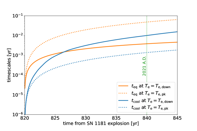
Figure 11: The time evolution of the heating (orange) and cooling (blue) timescales of the inner shocked ejecta, calculated for a parameter set $(\dot{M}_{\rm w},t_{\rm w},M_{\rm{ej}})=(1\times 10^{-6}~{}M_{\odot}\,\mathrm{yr}^{-1},820~{}\mathrm{yr},0.3~{}M_{\odot})$ using our dynamical model. The solid lines are for the immediate shock downstream with an electron temperature of $T_{\mathrm{e}}=T_{\mathrm{e,down}}$ and the dotted lines are estimated for a peak temperature of the cooling function $k_{\mathrm{B}}T_{\mathrm{e}}=k_{\mathrm{B}}T_{\mathrm{e,pk}}=3.7\,\mathrm{eV}$.

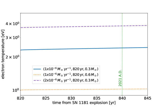
Figure 12: The time evolution of the emission temperature of the inner shocked SN ejecta obtained by the radiative shock condition (Eq. A5).

Although a radiative transfer calculation including the photo- and collisional ionization of the downstream plasma is required to accurately calculate the emission temperature, it can be roughly estimated in the radiative shock limit from the following condition;

$$\mathrm{EM}_{\rm ej}\Lambda(T_{\rm e})\approx 2\pi r_{\rm sh}^{2}\rho_{\rm ej}(r_{\mathrm{ej}})v_{\rm sh}^{3},$$ (A5)

where

$$\mathrm{EM}_{\rm ej}=n_{\rm e}n_{\rm ion}V_{\rm sh,ej}=\frac{\rho_{\rm ej}^{2}V_{\rm sh,ej}}{\mu_{\rm e}\mu_{\rm ion}m_{\rm u}^{2}},$$ (A6)

is the emission measure of the shocked ejecta with

$$V_{\mathrm{sh,ej}}\approx\frac{4}{3}\pi\left(r_{\mathrm{in,f}}^{3}-r_{\mathrm{sh}}^{3}\right)=\frac{4}{3}\pi r_{\mathrm{sh}}^{3}\left[\left(\frac{2\gamma}{1+\gamma}\right)^{3}-1\right]$$ (A7)

being its volume. The left and right hand sides of Eq. (A5) represent the emission luminosity of and the energy injection rate into the shocked ejecta. Figure 12 shows the emission temperature obtained from Eq. (A5) for several sets of model parameters. As expected from the timescale arguments above, the emission temperature is in the range of $\lesssim 3\mbox{--}4\,\mathrm{eV}$, suggesting that the inner shocked SN ejecta emit mainly UV photons, not X rays. These UV photons are expected to be absorbed by the surrounding dust-rich ring and re-emitted in the IR bands.

References

- Arnaud (1996) Arnaud, K. A. 1996, in Astronomical Society of the Pacific Conference Series, Vol. 101, Astronomical Data Analysis Software and Systems V, ed. G. H. Jacoby & J. Barnes, 17
- Bailer-Jones et al. (2021) Bailer-Jones, C. A. L., Rybizki, J., Fouesneau, M., Demleitner, M., & Andrae, R. 2021, AJ, 161, 147, doi: 10.3847/1538-3881/abd806
- Bartalucci et al. (2014) Bartalucci, I., Mazzotta, P., Bourdin, H., & Vikhlinin, A. 2014, ¥aap, 566, A25, doi: 10.1051/0004-6361/201423443
- Cash (1979) Cash, W. 1979, ApJ, 228, 939, doi: 10.1086/156922
- Chevalier (1982) Chevalier, R. A. 1982, ApJ, 258, 790, doi: 10.1086/160126
- Chevalier & Fransson (1992) Chevalier, R. A., & Fransson, C. 1992, ApJ, 395, 540, doi: 10.1086/171674
- Chevalier & Soker (1989) Chevalier, R. A., & Soker, N. 1989, ApJ, 341, 867, doi: 10.1086/167545
- Colgate & McKee (1969) Colgate, S. A., & McKee, C. 1969, ApJ, 157, 623, doi: 10.1086/150102
- de Vries et al. (2015) de Vries, C. P., den Herder, J. W., Gabriel, C., et al. 2015, A&A, 573, A128, doi: 10.1051/0004-6361/201423704
- den Herder et al. (2001) den Herder, J. W., Brinkman, A. C., Kahn, S. M., et al. 2001, A&A, 365, L7, doi: 10.1051/0004-6361:20000058
- Evans et al. (2014) Evans, P. A., Osborne, J. P., Beardmore, A. P., et al. 2014, ApJS, 210, 8, doi: 10.1088/0067-0049/210/1/8
- Fesen et al. (2023) Fesen, R. A., Schaefer, B. E., & Patchick, D. 2023, arXiv e-prints, arXiv:2301.04809, doi: 10.48550/arXiv.2301.04809
- Fink et al. (2014) Fink, M., Kromer, M., Seitenzahl, I. R., et al. 2014, MNRAS, 438, 1762, doi: 10.1093/mnras/stt2315
- Foley et al. (2013) Foley, R. J., Challis, P. J., Chornock, R., et al. 2013, ApJ, 767, 57, doi: 10.1088/0004-637X/767/1/57
- Foster et al. (2012) Foster, A. R., Ji, L., Smith, R. K., & Brickhouse, N. S. 2012, ApJ, 756, 128, doi: 10.1088/0004-637X/756/2/128
- Fruscione et al. (2006) Fruscione, A., McDowell, J. C., Allen, G. E., et al. 2006, in Observatory Operations: Strategies, Processes, and Systems, ed. D. R. Silva & R. E. Doxsey, Vol. 6270, International Society for Optics and Photonics (SPIE), 586 – 597, doi: 10.1117/12.671760
- Gabriel et al. (2004) Gabriel, C., Denby, M., Fyfe, D. J., et al. 2004, in Astronomical Society of the Pacific Conference Series, Vol. 314, Astronomical Data Analysis Software and Systems (ADASS) XIII, ed. F. Ochsenbein, M. G. Allen, & D. Egret, 759
- Gaia Collaboration et al. (2021) Gaia Collaboration, Brown, A. G. A., Vallenari, A., et al. 2021, A&A, 649, A1, doi: 10.1051/0004-6361/202039657
- Garmire (1997) Garmire, G. P. 1997, in American Astronomical Society Meeting Abstracts, Vol. 190, American Astronomical Society Meeting Abstracts #190, 34.04
- Gvaramadze et al. (2019) Gvaramadze, V. V., Gräfener, G., Langer, N., et al. 2019, Nature, 569, 684, doi: 10.1038/s41586-019-1216-1
- Hamilton et al. (1983) Hamilton, A. J. S., Sarazin, C. L., & Chevalier, R. A. 1983, ApJS, 51, 115, doi: 10.1086/190841
- HEASARC (2014) HEASARC. 2014, HEAsoft: Unified Release of FTOOLS and XANADU. http://ascl.net/1408.004
- Iben & Tutukov (1984) Iben, I., J., & Tutukov, A. V. 1984, ApJS, 54, 335, doi: 10.1086/190932
- Jansen et al. (2001) Jansen, F., Lumb, D., Altieri, B., et al. 2001, A&A, 365, L1, doi: 10.1051/0004-6361:20000036
- Kasen (2010) Kasen, D. 2010, ApJ, 708, 1025, doi: 10.1088/0004-637X/708/2/1025
- Kashiyama et al. (2019) Kashiyama, K., Fujisawa, K., & Shigeyama, T. 2019, ApJ, 887, 39, doi: 10.3847/1538-4357/ab4e97
- Kashyap et al. (2018) Kashyap, R., Haque, T., Lorén-Aguilar, P., García-Berro, E., & Fisher, R. 2018, ApJ, 869, 140, doi: 10.3847/1538-4357/aaedb7
- Kirchschlager et al. (2019) Kirchschlager, F., Schmidt, F. D., Barlow, M. J., et al. 2019, MNRAS, 489, 4465, doi: 10.1093/mnras/stz2399
- Kromer et al. (2013) Kromer, M., Fink, M., Stanishev, V., et al. 2013, MNRAS, 429, 2287, doi: 10.1093/mnras/sts498
- Kuntz & Snowden (2008) Kuntz, K. D., & Snowden, S. L. 2008, A&A, 478, 575, doi: 10.1051/0004-6361:20077912
- Kuriyama & Shigeyama (2020) Kuriyama, N., & Shigeyama, T. 2020, A&A, 635, A127, doi: 10.1051/0004-6361/201937226
- Livne et al. (2005) Livne, E., Asida, S. M., & Höflich, P. 2005, ApJ, 632, 443, doi: 10.1086/432975
- Lykou et al. (2022) Lykou, F., Parker, Q. A., Ritter, A., et al. 2022, arXiv e-prints, arXiv:2208.03946, doi: 10.48550/arXiv.2208.03946
- Masai (1994) Masai, K. 1994, ApJ, 437, 770, doi: 10.1086/175037
- Matzner & McKee (1999) Matzner, C. D., & McKee, C. F. 1999, ApJ, 510, 379, doi: 10.1086/306571
- Moriya et al. (2013) Moriya, T. J., Maeda, K., Taddia, F., et al. 2013, MNRAS, 435, 1520, doi: 10.1093/mnras/stt1392
- Nomoto & Iben (1985) Nomoto, K., & Iben, I., J. 1985, ApJ, 297, 531, doi: 10.1086/163547
- Oskinova et al. (2020) Oskinova, L. M., Gvaramadze, V. V., Gräfener, G., Langer, N., & Todt, H. 2020, A&A, 644, L8, doi: 10.1051/0004-6361/202039232
- Ritter et al. (2021) Ritter, A., Parker, Q. A., Lykou, F., et al. 2021, ApJ, 918, L33, doi: 10.3847/2041-8213/ac2253
- Saio & Nomoto (1985) Saio, H., & Nomoto, K. 1985, A&A, 150, L21
- Schaefer (2023) Schaefer, B. E. 2023, arXiv e-prints, arXiv:2301.04807, doi: 10.48550/arXiv.2301.04807
- Schwab et al. (2016) Schwab, J., Quataert, E., & Kasen, D. 2016, MNRAS, 463, 3461, doi: 10.1093/mnras/stw2249
- Shen (2015) Shen, K. J. 2015, ApJ, 805, L6, doi: 10.1088/2041-8205/805/1/L6
- Smith & Hughes (2010) Smith, R. K., & Hughes, J. P. 2010, ApJ, 718, 583, doi: 10.1088/0004-637X/718/1/583
- Snowden et al. (2004) Snowden, S. L., Collier, M. R., & Kuntz, K. D. 2004, ApJ, 610, 1182, doi: 10.1086/421841
- Spitzer (1956) Spitzer, L. 1956, Physics of Fully Ionized Gases (Interscience Publishers)
- Strüder et al. (2001) Strüder, L., Briel, U., Dennerl, K., et al. 2001, A&A, 365, L18, doi: 10.1051/0004-6361:20000066
- Suzuki et al. (2021) Suzuki, H., Plucinsky, P. P., Gaetz, T. J., & Bamba, A. 2021, ¥aap, 655, A116, doi: 10.1051/0004-6361/202141458
- Tsuna et al. (2020) Tsuna, D., Ishii, A., Kuriyama, N., Kashiyama, K., & Shigeyama, T. 2020, ApJ, 897, L44, doi: 10.3847/2041-8213/aba0ac
- Tsuna et al. (2019) Tsuna, D., Kashiyama, K., & Shigeyama, T. 2019, ApJ, 884, 87, doi: 10.3847/1538-4357/ab40ba
- Tsuna et al. (2021a) —. 2021a, ApJ, 914, 64, doi: 10.3847/1538-4357/abfaf8
- Tsuna et al. (2021b) Tsuna, D., Takei, Y., Kuriyama, N., & Shigeyama, T. 2021b, PASJ, 73, 1128, doi: 10.1093/pasj/psab063
- Turner et al. (2001) Turner, M. J. L., Abbey, A., Arnaud, M., et al. 2001, A&A, 365, L27, doi: 10.1051/0004-6361:20000087
- Wu et al. (2023) Wu, C., Xiong, H., Lin, J., et al. 2023, ApJ, 944, L54, doi: 10.3847/2041-8213/acb6f3
- Yao et al. (2023) Yao, P. Z., Quataert, E., & Goulding, A. 2023, arXiv e-prints, arXiv:2302.07886, doi: 10.48550/arXiv.2302.07886