Recognizable Information Bottleneck

Abstract

Information Bottlenecks (IBs) learn representations that generalize to unseen data by information compression. However, existing IBs are practically unable to guarantee generalization in real-world scenarios due to the vacuous generalization bound. The recent PAC-Bayes IB uses information complexity instead of information compression to establish a connection with the mutual information generalization bound. However, it requires the computation of expensive second-order curvature, which hinders its practical application. In this paper, we establish the connection between the recognizability of representations and the recent functional conditional mutual information (f-CMI) generalization bound, which is significantly easier to estimate. On this basis we propose a Recognizable Information Bottleneck (RIB) which regularizes the recognizability of representations through a recognizability critic optimized by density ratio matching under the Bregman divergence. Extensive experiments on several commonly used datasets demonstrate the effectiveness of the proposed method in regularizing the model and estimating the generalization gap.

1 Introduction

Learning representations that are generalized to unseen data is one of the most fundamental goals for machine learning. The IB method Tishby et al. (2000) is one of the prevailing paradigms. It centers on learning representations that not only sufficiently retain information about the label, but also compress information about the input. The rationale behind the IB is that the information compression of representations penalizes complex hypotheses and guarantees generalization by a probability generalization bound Shamir et al. (2010); Vera et al. (2018). It is expected that one can obtain a lower generalization gap through optimizing the IB training objective. However, in finite and continuous data scenarios, such as an image classification task with deep neural networks (DNNs), this upper bound is dominated by a prohibitively large constant with any reasonable probability and becomes vacuous, thus making the information compression term negligible Rodriguez Galvez (2019). This deprives IB method of the theoretical guarantee in real-world scenarios.

Recently, motivated by the mutual information (MI)-based generalization bound in the information-theoretic framework Xu and Raginsky (2017), Wang et al. (2022) proposed to use the information stored in weights, i.e., the MI between the input dataset and the output weights of the algorithm, to replace the compression term in the IB objective. It is worth noting, however, that the MI-based generalization bound may still be vacuous due to the fact that the MI can easily go to infinity, e.g., in cases where the learning algorithm is a deterministic function of the input data Bu et al. (2020); Steinke and Zakynthinou (2020). More importantly, it is notoriously difficult to estimate the MI between two high-dimensional random variables, e.g., weights of model and a training dataset. Although one can recover non-vacuous bound by restricting the prior and posterior of the weights to Gaussian distributions Dziugaite and Roy (2017); Wang et al. (2022), the computational burdens (from e.g., Monte-Carlo sampling or calculating the second-order curvature information) are still cumbersome.

To address the unbounded nature of MI-based bound, Steinke and Zakynthinou (2020) proposed the celebrated conditional mutual information (CMI) generalization bound, which normalizes each datum to one bit, thus is always bounded. The intuition is that measuring information that “recognizes” an input sample is much simpler than measuring information that “reconstructs” an input sample. Harutyunyan et al. (2021) further extended this idea to a black-box algorithm setting and proposed a functional CMI (f-CMI) generalization bound, which significantly reduces the computational cost by computing the CMI with respect to the low-dimensional predictions rather than the high-dimensional weights. This inspires us to consider the DNN encoder as a black box and the representation as the output predictions, which coincides with the original IB setting. Unfortunately, the computation of the f-CMI bound requires multiple runs on multiple draws of data, there is not yet a practical optimization algorithm to incorporate it into the training of the models.

In this paper, we first formulate the recognizability from the perspective of binary hypothesis testing (BHT) and show the connection between the recognizability of representations and the f-CMI generalization bound. Based on the reasoning that lower recognizability leads to better generalization, we propose a new IB objective, called the Recognizable Information Bottleneck (RIB). A recognizability critic is exploited to optimize the RIB objective using density ratio matching under the Bregman divergence. Extensive experiments on several commonly used datasets demonstrate the effectiveness of the RIB in controlling generalization and the potential of estimating the generalization gap for the learned models using the recognizability of representations.

Our main contributions can be concluded as follows:

• We define a formal characterization of recognizability and then show the connection between the recognizability of representations and the f-CMI bound.

• We propose the RIB objective to regularize the recognizability of representations.

• We propose an efficient optimization algorithm of RIB which exploits a recognizability critic optimized by density ratio matching.

• We empirically demonstrate the regularization effects of RIB and the ability of estimating the generalization gap by the recognizability of representations.

1.1 Other Related Work

1.1.1   Information bottlenecks

There have been numerous variants of IB Alemi et al. (2017); Kolchinsky et al. (2019); Gálvez et al. (2020); Pan et al. (2021); Yu et al. (2021) and have been utilized on a wide range of machine learning tasks Du et al. (2020); Lai et al. (2021); Li et al. (2022). However, one pitfall of IBs is that there may be no causal connection between information compression and generalization in real-world scenarios Saxe et al. (2018); Rodriguez Galvez (2019); Dubois et al. (2020). Wang et al. (2022) addressed this issue by introducing an information complexity term to replace the compression term, which turns out to be the Gibbs algorithm stated in the PAC-Bayesian theory Catoni (2007); Xu and Raginsky (2017).

1.1.2   Information-theoretical generalization bounds

The MI between the input and output of a learning algorithm has been widely used to bound the generalization error Xu and Raginsky (2017); Pensia et al. (2018); Negrea et al. (2019); Bu et al. (2020). To tackle the intrinsic defects of MI, Steinke and Zakynthinou (2020) proposed the CMI generalization bound, then Haghifam et al. (2020) proved that the CMI-based bounds are tighter than MI-based bounds. Zhou et al. (2022) made the CMI bound conditioned on an individual sample and obtained a tighter bound. The above bounds are based on the output of the algorithm (e.g. weights of the model) rather than information of predictions which is much easier to estimate in practice Harutyunyan et al. (2021).

2 Preliminaries

2.1 Notation and Definitions

We use capital letters for random variables, lower-case letters for realizations and calligraphic letters for domain. Let $X$ and $Y$ be random variables defined on a common probability space, the mutual information between $X$ and $Y$ is defined as $I(X;Y)=D_{\mathrm{KL}}(P_{X,Y}\|P_{X}\otimes P_{Y})$, where $D_{\mathrm{KL}}$ is the Kullback-Leibler (KL) divergence. The conditional mutual information is defined as $I(X;Y|Z)=D_{\mathrm{KL}}(P_{X,Y|Z}\|P_{X|Z}P_{Y|Z}|P_{Z})=\mathbb{E}_{z\sim P_{Z}}\left[I(X;Y|Z=z)\right]$. A random variable $X$ is $\sigma$-subgaussian if $\mathbb{E}\left[\exp(\lambda(X-\mathbb{E}(X)))\right]\leq\exp\left({\lambda^{2}\sigma^{2}}/{2}\right)$ for all $\lambda\in\mathbb{R}$.

Throughout this paper, we consider the supervised learning setting. There is an instance random variable $X$, a label random variable $Y$, an unknown data distribution $\mathcal{D}$ over the $\mathcal{Z}=\mathcal{X}\times\mathcal{Y}$ and a training dataset $S=(Z_{1},Z_{2},\dots,Z_{n})\sim\mathcal{D}^{n}$ consisting of $n$ i.i.d. samples drawn from the data distribution. There is a learning algorithm $A:\mathcal{Z}^{n}\rightarrow\mathcal{W}$ and an encoder function $f_{\theta}:\mathcal{X}\rightarrow\mathcal{T}$ from its class $\mathcal{F}:=\{T=\mathbb{E}_{X}[\mathbf{1}[t=f_{\theta}(X)]]:\theta\in\mathcal{W}\}$. We assume that $\mathcal{T}$ is of finite size and consider $T$ as the representation. We define two expressions of generalization, one from the “weight” perspective and one from the “representation” perspective:

1. Given a loss function $\ell:\mathcal{W}\times\mathcal{Z}\rightarrow\mathbb{R}$, the true risk of the algorithm $A$ w.r.t. $\ell$ is $\mathcal{L}(w,S)=\mathbb{E}_{z^{\prime}\sim\mathcal{D}}\ell(w,z^{\prime})$ and the empirical risk of the algorithm $A$ w.r.t. $\ell$ is $\mathcal{L}_{\mathrm{emp}}(w,S)=\frac{1}{n}\sum_{i=1}^{n}\ell(w,z_{i})$. The generalization error is defined as $\mathrm{gen}(w,S)=\mathcal{L}(w,S)-\mathcal{L}_{\mathrm{emp}}(w,S)$;

2. Given a loss function $\ell:\mathcal{T}\times\mathcal{Y}\rightarrow\mathbb{R}$, the true risk of the algorithm $A$ w.r.t. $\ell$ is $\mathcal{L}(T,Y)=\mathbb{E}_{z^{\prime}\sim\mathcal{D}}\ell(t^{\prime},y^{\prime})$ and the empirical risk of the algorithm $A$ w.r.t. $\ell$ is $\mathcal{L}_{\mathrm{emp}}(T,Y)=\frac{1}{n}\sum_{i=1}^{n}\ell(t_{i},y_{i})$. The generalization error is defined as $\mathrm{gen}(T,Y)=\mathcal{L}(T,Y)-\mathcal{L}_{\mathrm{emp}}(T,Y)$.

2.2 Generalization Guarantees for Information Bottlenecks

The IB method Tishby et al. (2000) wants to find the optimal representation by minimizing the following Lagrangian:

$$\mathcal{L}_{\mathrm{IB}}=\mathcal{L}_{\mathrm{emp}}(T,Y)+\beta I(T;X),$$ (1)

where $\beta$ is the Lagrange multiplier. The $I(T;X)$ in Eq. 1 can be seen as a compression term that regularizes the complexity of $T$. It has been demonstrated to upper-bound the generalization error Shamir et al. (2010); Vera et al. (2018). Concretely, for any given $\delta>0$, with probability at least $1-\delta$ it holds that

$$\left|\mathrm{gen}(T,Y)\right|\leq\mathcal{O}(\frac{\log n}{\sqrt{n}})\sqrt{I(T;X)}+C_{\delta},$$

where $C_{\delta}=\mathcal{O}(|\mathcal{T}|/\sqrt{n})$ is a constant that depends on the cardinality of the space of $T$. The bound implies that the less information the representations can provide about the instances, the better the generalization of the algorithm. However, since $|\mathcal{T}|$ will become prohibitively large with any reasonable choice of $\delta$, this bound is actually vacuous in practical scenarios Rodriguez Galvez (2019).

A recent approach PAC-Bayes IB (PIB) Wang et al. (2022) tried to amend the generalization guarantee of IB by replacing the compression term with the information stored in weights, which leads to the following objective:

$$\mathcal{L}_{\mathrm{PIB}}=\mathcal{L}_{\mathrm{emp}}(w,S)+\beta I(w;S).$$

The rationale behind the PIB is stem from the input-output mutual information generalization bound which can also be derived from the PAC-Bayesian perspective Xu and Raginsky (2017); Banerjee and Montúfar (2021). Concretely, assume that the loss function $\ell(w,Z)$ is $\sigma$-subgaussian for all $w\in\mathcal{W}$, the expected generalization error can be upper-bounded by

$$\left|\mathbb{E}\left[\mathrm{gen}(w,S)\right]\right|\leq\sqrt{\frac{2\sigma^{2}}{n}I(W;S)}.$$

Intuitively, the bound implies that the less information the weight can provide about the input dataset, the better the generalization of the algorithm. However, as we mentioned above, the MI-based bound could be vacuous without proper assumptions and is hard to estimate for two high-dimensional variables such as the weight $W$ and the training dataset $S$.

2.3 The CMI-based Generalization Bounds

The CMI-based bounds Steinke and Zakynthinou (2020); Harutyunyan et al. (2021) characterize the generalization by measuring the ability of recognizing the input data given the algorithm output. This can be accomplished by recognizing the training samples from the “ghost” (possibly the test) samples. Formally, consider a supersample $\tilde{Z}\in\mathcal{Z}^{n\times 2}$ constructed from $n$ input samples mixed with $n$ ghost samples. A selector variable $U\sim\mathrm{Unif}(\{0,1\}^{n})$ selects the input samples from the supersample $\tilde{Z}$ to form the training set $S=\tilde{Z}_{U}=(\tilde{Z}_{i,U_{i}+1})_{i=1}^{n}$. Given a loss function $\ell(w,z)\in[0,1]$ for all $w\in\mathcal{W}$ and all $z\in\mathcal{Z}$, Steinke and Zakynthinou (2020) bound the expected generalization error by the CMI between the weight $W$ and the selector variable $U$ given the supersample $\tilde{Z}$:

$$\left|\mathbb{E}\left[\mathrm{gen}(w,S)\right]\right|\leq\sqrt{\frac{2}{n}I(W;U|\tilde{Z})}.$$ (2)

The intuition is that the less information the weight can provide to recognize input samples from their ghosts, the better the generalization of the algorithm. In this way, the algorithm that reveals a datum has only CMI of one bit, bounding the CMI by $n\log 2$, while the MI may be infinite. Harutyunyan et al. (2021) extended this idea to a black-box algorithm setting which measures the CMI with respect to the predictions of the model rather than the weight. It is able to further extend the prediction domain to the representation domain, which yields a setting similar to the original IB. Given a loss function $\ell(t,y)\in[0,1]$ for all $t\in\mathcal{T}$ and all $z\in\mathcal{Z}$, the expected generalization error is upper-bounded by the following f-CMI bound:

$$\left|\mathbb{E}\left[\mathrm{gen}(T,Y)\right]\right|\leq\sqrt{\frac{2}{n}I(T;U|\tilde{Z})}.$$ (3)

From the Markov chain $U\rightarrow W\rightarrow T$ and the data processing inequality, it follows that $I(T;U|\tilde{Z})\leq I(W;U|\tilde{Z})$, which indicates the bound in Eq. 3 is tighter than the bound in Eq. 2. Similarly, we can learn from the bound that the less information the representations can provide to recognize input samples from their ghosts, the better the generalization of the algorithm. Since the representation $T$ and the selector variable $U$ are relatively lower dimensional than the weight $W$ and the dataset $S$, respectively, estimating the f-CMI bound is far more efficient than the previous bounds.

3 Methodology

Although the f-CMI bound is theoretically superior to the generalization bounds of existing IBs, it has so far only been used as a risk certificate for the learned model Harutyunyan et al. (2021). Since computing the f-CMI bound requires multiple runs on multiple draws of data, there is no immediate way to incorporate it into the training of deep models. In this section, we first give a formal characterization of the recognizability and describe how to use the recognizability of representations to approximate the f-CMI bound. This motivates us to propose the RIB objective and an efficient optimization algorithm using a recognizability critic.

3.1 Recognizability

In order to characterize the recognizability, we first review some basic concepts of binary hypothesis testing (BHT) Levy (2008). Assume that there are two possible hypotheses, $H_{0}$ and $H_{1}$, corresponding to two possible distributions $P$ and $Q$ on a space $\mathcal{X}$, respectively,

$$H_{0}:X\sim P\qquad H_{1}:X\sim Q.$$

A binary hypothesis test between two distributions is to choose either $H_{0}$ or $H_{1}$ based on the observation of $X$. Given a decision rule $\Xi:\mathcal{X}\rightarrow\{0,1\}$ such that $\Xi=0$ denotes the test chooses $P$, and $\Xi=1$ denotes the test chooses $Q$. Then the recognizability can be defined as follows:

Definition 1 (Recognizability).

Let $H_{0},H_{1},P,Q,X,\Xi$ be defined as above. The recognizability between $P$ and $Q$ w.r.t. $\Xi$ for all randomized tests $P_{\Xi|X}$ is defined as

$$\Re_{\Xi}(P,Q):=\\ \lvert\left\{(\mathrm{Pr}(\Xi=1|H_{0}),\mathrm{Pr}(\Xi=1|H_{1}))\mid\forall\Xi\sim P_{\Xi|X}\right\}\rvert,$$

where $\mathrm{Pr}(\Xi=1|H_{0})$ is the probability of error given $H_{1}$ is true and $\mathrm{Pr}(\Xi=1|H_{1})$ is the probability of success given $H_{0}$ is true.

(a)

(b) $P\perp Q$

(c) $P=Q$

Figure 1: Illustrations of recognizability.

3.1.1   Remark

In words, the recognizability is the area of the achievable region for all tests drawn from $P_{\Xi|X}$ (see Fig. 1(a)). For BHT, one would like to select a test such that $\mathrm{Pr}(\Xi=1|H_{0})$ is as close to zero as possible while $\mathrm{Pr}(\Xi=1|H_{1})$ is as close to one as possible. However, the extreme case, i.e., $(\mathrm{Pr}(\Xi=1|H_{0})=0,\mathrm{Pr}(\Xi=1|H_{1})=1)$ or $(0,1)$, is achievable only if the hypotheses $H_{0}$ and $H_{1}$ are completely mutually exclusive, that is, $P$ is mutually singular w.r.t. $Q$, which indicates that the recognizability $\Re_{\Xi}(P,Q)=1$ (Fig. 1(b)). Similarly, when $H_{0}$ and $H_{1}$ are equivalent, that is, $P$ and $Q$ are identical, we have the recognizability $\Re_{\Xi}(P,Q)=0$ (Fig. 1(c)).

By the celebrated Neyman-Pearson lemma, we have that log-likelihood ratio testing (LRT) is the optimal decision rule, which means all the points in the achievable region are attained by LRT Neyman et al. (1933). It is also well-known that the upper boundary between the achievable and unachievable region is the receiver operating characteristic (ROC) of LRT Levy (2008). Therefore, given a LRT decision rule $\xi:\mathcal{X}\rightarrow[0,1]$, the recognizability w.r.t. $\xi$ can be computed by

$$\Re_{\xi}(P,Q)=2\times\mathrm{AUCROC}_{\xi}-1,$$ (4)

where $\mathrm{AUCROC}_{\xi}$ is the area under the ROC curve of $\xi$.

The formulation of recognizability offers us some fresh insights to consider generalization from the perspective of BHT, which leads to a new approach to regularization. Concretely, we rewrite the f-CMI term in Eq. 3 as

$$I(T;U|\tilde{Z}) =\mathbb{E}_{\tilde{z}\sim\tilde{Z}}D_{\mathrm{KL}}(P_{T,U|\tilde{Z}=\tilde{z}}\|P_{T|\tilde{Z}=\tilde{z}}\otimes P_{U})$$

$$=\mathbb{E}_{\tilde{z}\sim\tilde{Z}}D_{\mathrm{KL}}(P_{T|U,\tilde{Z}=\tilde{z}}\|P_{T|\tilde{Z}=\tilde{z}}),$$ (5)

where Section 3.1.1 follows by the uniformity of $U$. Consider a realization of supersample $\tilde{z}$. Let $t_{1},t_{2},\dots,t_{n}$ be a sequence drawn i.i.d. according to $P_{T|U,\tilde{Z}=\tilde{z}}$, then by the weak law of large numbers we have that

$$\frac{1}{n}\sum_{i=1}^{n}\log\frac{P_{T|U,\tilde{Z}=\tilde{z}}(t_{i})}{P_{T|\tilde{Z}=\tilde{z}}(t_{i})}\rightarrow D_{\mathrm{KL}}(P_{T|U,\tilde{Z}=\tilde{z}}\|P_{T|\tilde{Z}=\tilde{z}}).$$

This suggests that the log-likelihood ratio between the distributions $P_{T|U,\tilde{Z}=\tilde{z}}$ and $P_{T|\tilde{Z}=\tilde{z}}$ amounts to the KL divergence, and eventually an estimate of $I(T;U|\tilde{z})$, which is the single-draw of the f-CMI bound. Thus, the more similar these two distributions are, the more difficult it is for us to determine which hypothesis $t_{i}$ originates from by LRT, namely, the lower the recognizability; we can also verify, in turn, that the KL divergence is minimal when we achieve the lowest recognizability (Fig. 1(c)). To make this explicit, we theoretically establish the connection between recognizability of representations and the f-CMI bound through the following theorem.

Theorem 1.

Let $\tilde{z}$ be a realization of supersample $\tilde{Z}$, $T$ be the representation variable defined as above, $\xi:\mathcal{T}\rightarrow[0,1]$ be the LRT decision rule and $U\sim\mathrm{Unif}(\{0,1\}^{n})$. The recognizability of representations $\Re_{\xi}(P_{T|\tilde{Z}=\tilde{z}},P_{T|U,\tilde{Z}=\tilde{z}})$ is upper bound by $I(T;U|\tilde{z})+\log\frac{e}{2}$.

Proof.

See Appendix A. ∎

Inspired by the above insights, we propose the RIB to constrain the model to learn representations having low recognizability, which utilizes a log-likelihood ratio estimator that we name recognizability critic. We will detail it in the next subsection.

3.2 Recognizable Information Bottleneck

We first define a new objective function that takes the recognizability of representations into consideration. Let $\tilde{z}$ be a realization of $\tilde{Z}$ which is composed of a training set $S$ of size $n$ and a ghost set $\bar{S}$ of the same size, $U\sim\mathrm{Unif}(\{0,1\}^{n})$ be a random variable indicating the set from which the instance of representation comes. Note that in general the ghost set is built from the validation or test (if available) set with dummy labels, and we will experiment later with ghost from different sources. Now we can write a new IB objective called the Recognizable Information Bottleneck (RIB) as follows:

$$\mathcal{L}_{\mathrm{RIB}}=\mathcal{L}_{\mathrm{emp}}(T,Y)+\beta I(T;U|\tilde{z}),$$ (6)

where the first term enforces empirical risk minimization, the second term regularizes the recognizability of representations and $\beta$ is the trade-off parameter.

To optimize the second term of Eq. 6, we first train a log-likelihood ratio estimator $V_{\phi}:\mathcal{T}^{2}\rightarrow\mathbb{R}$ that we call the recognizability critic. It takes a pair of representations as input, one obtained from the training set $S$ samples and the other from the ghost set $\bar{S}$. The pair of representations is then randomly concatenated and treated as a single draw from the joint distribution $P_{T,U|\tilde{Z}=\tilde{z}}$, since the probability of occurrence of the possible outcomes is consistent. Next we train the recognizability critic by maximizing the lower bound on the Jensen-Shannon divergence as suggested in Hjelm et al. (2019); Poole et al. (2019) by the following objective:

$$\max_{\phi}\mathbb{E}_{\tilde{t}\sim P_{T|U,\tilde{Z}=\tilde{z}}}[-\mathrm{sp}(-V_{\phi}(\tilde{t}))]\\ -\mathbb{E}_{\tilde{t}\sim P_{T|\tilde{Z}=\tilde{z}}}[\mathrm{sp}(V_{\phi}(\tilde{t}))],$$ (7)

where $\mathrm{sp}(x)=\log(1+e^{x})$ is the softplus function. Once the critic $V$ reaches the maximum, we can obtain the density ratio by

$$R(\tilde{t})=\frac{P_{T|U,\tilde{Z}=\tilde{z}}(\tilde{t})}{P_{T|\tilde{Z}=\tilde{z}}(\tilde{t})}\approx\exp(V_{\phi}(\tilde{t})).$$

Since the lowest recognizability achieves when the two distributions are identical, that is, the density ratio $R^{*}\equiv 1$, to regularize the representations, we use a surrogate loss motivated by density-ratio matching Sugiyama et al. (2012), which optimizes the Bregman divergence between the optimal density ratio $R^{*}$ and the estimated density ratio $R(\tilde{t})$ defined as

$$D_{\mathrm{BR}_{F}}(R^{*}\|R(\tilde{t})):=F(R^{*})-F(R(\tilde{t}))-\partial F(R(\tilde{t}))(R^{*}-R(\tilde{t})).$$ (8)

Here, $F$ is a differentiable and strictly convex function and $\partial F$ is its derivative. We can derive different measures by using different $F$. In the experiments we use $F(R)=R\log R-(1+R)\log(1+R)$, at which point the Bregman divergence is reduced to the binary KL divergence. More examples and comparison results are given in Appendix C.

Now the objective function for the encoder $f_{\theta}$ can be written as

$$\min_{\theta}\frac{1}{n}\sum_{i=1}^{n}\ell(t_{i},y_{i})+\beta D_{\mathrm{BR}}(R^{*}\|R(\tilde{t}_{i})).$$ (9)

The complete optimization algorithm is described in Algorithm 1. Note that although it is also feasible to directly minimize Eq. 7 with respect to the encoder parameter $\theta$ which leads to a minimax game similar to GAN Goodfellow et al. (2014); Nowozin et al. (2016), we empirically find that this may cause training instability especially when data is scarce (as detailed in the next section). We consider this is due to the randomness of $U$ which leads to large variance gradients and hinders the convergence of the model, while we utilize a fixed ratio for optimization thus it is not affected.

When the recognizability critic finishes training, we can obtain the class probability from the estimated density ratio via the sigmoid function, which gives us the following decision rules:

$$\hat{\xi}(\tilde{t})=\frac{1}{1+\exp(-R(\tilde{t}))}.$$

Then the recognizability of representations can be estimated based on the outputs of $\hat{\xi}$ via Eq. 4. We find that the recognizability of representations can be used as an indicator of the generalizability and achieve comparable performance to the f-CMI bound, which will be discussed in the next section.

Algorithm 1 Optimization of Recognizable Information Bottleneck (RIB)

Input: training set $S=\{(x_{i},y_{i})\}_{i=1}^{N}$, ghost set $\bar{S}=\{\bar{x}_{i}\}_{i=1}^{N}$, encoder $f_{\theta}$, initial encoder parameter $\theta_{0}$, recognizability critic $V_{\phi}$, initial recognizability critic parameter $\phi_{0}$, batch size $B$, learning rate $\eta$
Output: trained encoder parameter $\theta$, trained recognizability critic parameter $\phi$

1:  initialize: $\theta\leftarrow\theta_{0},\phi\leftarrow\phi_{0}$

2:  while not converged do

3:     sample training mini-batch $\{(x_{i},y_{i})\}_{i=1}^{B}\sim S$

4:     sample ghost mini-batch $\{\bar{x}_{i}\}_{i=1}^{B}\sim\bar{S}$

5:     sample $\{u_{i}\}_{i=1}^{B}\sim\mathrm{Unif}(\{0,1\})$

6:     compute $\{t_{i}=f_{\theta}(x_{i})\}_{i=1}^{B},\{\bar{t}_{i}=f_{\theta}(\bar{x}_{i})\}_{i=1}^{B}$

7:     set $\tilde{t}=\{\tilde{t}_{i}\}_{i=1}^{B}$, where $\tilde{t}_{i}=\begin{cases}t_{i}\circ\bar{t}_{i},&u_{i}=0\\ \bar{t}_{i}\circ t_{i},&u_{i}=1\end{cases}$

8:     compute gradient $g_{\phi}$ by Eq. 7 and update $\phi$:$\phi\leftarrow\phi+\eta g_{\phi}$

9:     compute gradient $g_{\theta}$ by Eq. 9 and update $\theta$:$\theta\leftarrow\theta-\eta g_{\theta}$

10:  end while

11:  return ($\theta,\phi$)

Method	Fashion			SVHN			CIFAR10
	1250	5000	20000	1250	5000	20000	1250	5000	20000
CE	18.61±0.87	14.57±0.47	10.18±0.34	30.03±1.04	19.51±0.52	11.77±0.33	61.51±1.13	50.22±0.81	32.81±0.70
L2	18.54±0.66	14.81±0.39	10.57±0.50	29.60±1.00	19.30±0.73	11.19±0.22	61.62±0.97	49.89±0.93	32.41±1.17
Dropout	18.58±0.57	14.58±0.51	10.20±0.40	29.68±0.94	19.40±0.57	11.82±0.42	61.53±0.95	50.02±0.78	32.69±0.47
VIB	17.57±0.44	13.86±0.35	9.64±0.24	40.54±5.75	18.93±0.61	11.28±0.23	59.77±0.78	49.14±0.60	31.82±0.39
NIB	18.30±0.42	14.34±0.29	9.94±0.21	29.34±0.71	19.44±0.38	11.59±0.24	61.00±0.77	50.01±0.57	32.32±0.41
DIB	18.11±0.37	13.99±0.34	9.74±0.27	29.95±0.93	19.37±0.62	11.54±0.23	61.02±0.70	50.09±0.66	32.36±0.49
PIB	18.44±0.52	14.33±0.29	10.00±0.23	29.40±0.78	19.40±0.61	11.60±0.27	61.19±0.82	50.09±0.79	32.48±0.31
RIB	17.05±0.41	13.57±0.28	9.32±0.25	27.72±1.17	17.37±0.52	10.80±0.27	59.16±1.17	47.57±0.60	31.06±0.38

Table 1: Comparison of the mean test error (%) on three datasets with different training set sizes.

4 Experiments

In this section, we demonstrate the effectiveness of RIB as a training objective to regularize the DNNs and verify the capability of recognizability critic to estimate generalization gap. Code is available at https://github.com/lvyilin/RecogIB.

4.1 Experimental Setup

4.1.1   Datasets

Our experiments mainly conduct on three widely-used datasets: Fashion-MNIST Xiao et al. (2017), SVHN Netzer et al. (2011) and CIFAR10 Krizhevsky et al. (2009). We also give the results on MNIST and STL10 Coates et al. (2011) in Appendix C. We adopt the data setting of Harutyunyan et al. (2021) to enable the calculation and comparison of f-CMI bound. Concretely, each experiment is conducted on $k_{1}$ draws of the original training set (to form a supersample $\tilde{z}$) and $k_{2}$ draws of the train-val-split (i.e., $k_{1}k_{2}$ runs in total), which correspond to the randomness of $\tilde{Z}$ and $T$, respectively. In all our experiments, $k_{1}=k_{2}=5$. Unless otherwise stated, the validation set is used as the ghost set. To demonstrate the effectiveness across different data scales, we perform sub-sampling on the training set with different sizes $n\in\{1250,5000,20000\}$.

4.1.2   Implementation details

We use a DNN model composed of a 4-layer CNN (128-128-256-1024) and a 2-layer MLP (1024-512) as the encoder, and use a 4-layer MLP (1024-1024-1024-1) as the recognizability critic. We train the learning model using Adam optimizer Kingma and Ba (2015) with betas of (0.9, 0.999) and train the recognizability critic using SGD with momentum of 0.9 as it is more stable in practice. All learning rates are set to 0.001, and the models are trained 100 epochs using the cosine annealing learning rate scheme with a batch size of 128. The trade-off parameter $\beta$ is selected from $\{10^{-1},10^{0},10^{1},10^{2}\}$ according to the desired regularization strength as discussed later. All the experiments are implemented with PyTorch and performed on eight NVIDIA RTX A4000 GPUs. More experimental details are provided in Appendix B.

4.2 Regularization Effects of RIB

We report the average performance of RIB over $k_{1}k_{2}$ draws to show its regularization effects on different data scales. We use cross entropy (CE) loss as the baseline. Furthermore, we compare with two common regularization methods: L2 normalization and dropout Srivastava et al. (2014). The strength of the L2 normalization is set to 1e-4 and the dropout rate is set to 0.1. We also compare with four popular IB counterparts: VIB Alemi et al. (2017), NIB Kolchinsky et al. (2019), DIB Yu et al. (2021), and PIB Wang et al. (2022). All methods impose regularization on the representations, except for PIB which is on the weights. Their regularization strength is determined by the best result of $\{10^{-5},10^{-4},\dots,10^{1}\}$. Table 1 shows that RIB consistently outperforms the compared methods across all datasets and all training set sizes. This demonstrates that regularizing the recognizability of representations as well as reducing the recognizable information contributes significantly to improving the generalization of the model. Another point worth mentioning is that the performance of PIB does not outperform VIB and its variants. We consider that this is because the PIB computes the gradient for the overall data only once per epoch, in order to maintain an affordable computational complexity, while representation-based regularization methods compute the gradient for each iteration efficiently, thus provide more fine-grained information for model training. Furthermore, we credit the improvement of RIB over VIB and its variants to the use of the ghost set, which enables the computation of recognizable information, and the reduction of recognizability of representations to facilitate generalization.

Source	1250	5000	20000
SVHN	61.26±1.20	51.59±0.97	37.13±0.94
CIFAR100	60.31±0.91	49.20±0.78	33.27±0.61
CIFAR10	59.16±1.17	47.57±0.60	31.06±0.38
Baseline	61.51±1.13	50.22±0.81	32.81±0.70

Table 2: Comparison of the mean test error (%) using CIFAR10 as the training data and constructing ghosts with different sources.

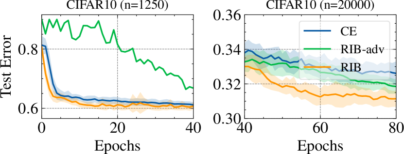
Figure 2: Mean test risk curves on CIFAR10 with training set sizes of 1250 and 20000. “RIB-adv” represents optimizing the RIB objective with adversarial training.

4.2.1   Effectiveness of the surrogate loss

We first examine whether optimizing the Bregman divergence of Eq. 8 is better than optimizing Eq. 7 by adversarial training method using Jensen-Shannon divergence Nowozin et al. (2016). The risk curves are illustrated in Fig. 2. We find that: i) training RIB in an adversarial manner may produce unstable gradients when the data is scarce thus making the model difficult to converge; ii) with more data, “RIB-adv” can also regularize the model and perform better than the CE baseline; and iii) the RIB optimized by our surrogate loss consistently outperforms the baselines at different data scales, which demonstrates its effectiveness on regularizing the DNNs.

4.2.2   Results of ghosts with different sources

Although the construction of the ghost set is supposed to be performed on a supersample drawn from a single data domain, it is intriguing to investigate whether it can still achieve similar performance with different data sources. We use the CIFAR10 as the training set and construct the ghost from three sources: i) SVHN, distinct from CIFAR10; ii) CIFAR100 Krizhevsky et al. (2009), similar to CIFAR10 but with more categories and iii) CIFAR10 for comparison. Table 2 shows that i) the more similar the sources are to the training set, the more effective the regularization will be. This is reasonable because recognizing samples from other domains may be too simple thus not provide useful information. More similar sources can provide more fine-grained recognizable information that is of more benefit to the model. ii) Nevertheless, even data from different sources, such as SVHN, can still provide valuable information to improve generalization when training data is scarce (e.g., $n=1250$).

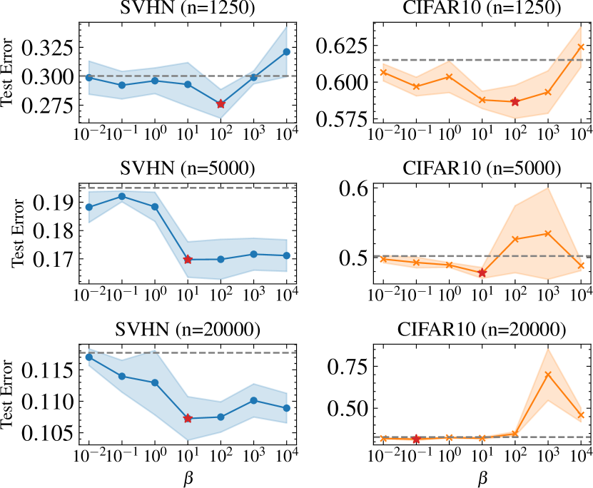
Figure 3: Impact of $\beta$ on mean test risk with different training set sizes. The horizontal dashed line indicates the performance on CE baseline. The star marker indicates the best result.

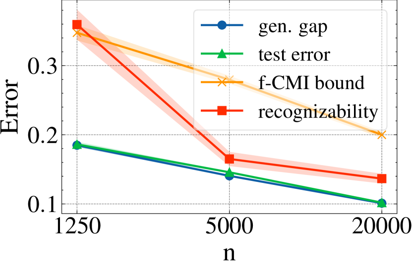
(a) Fashion

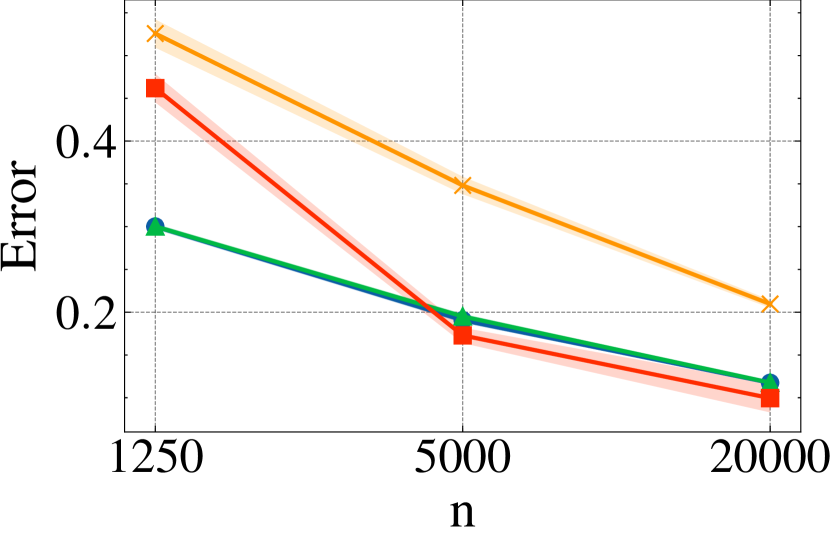
(b) SVHN

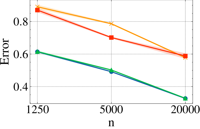
(c) CIFAR10

Figure 4: Comparison of expected generalization gap, mean test error, f-CMI bound and recognizability of representations on three datasets with varying training set sizes.

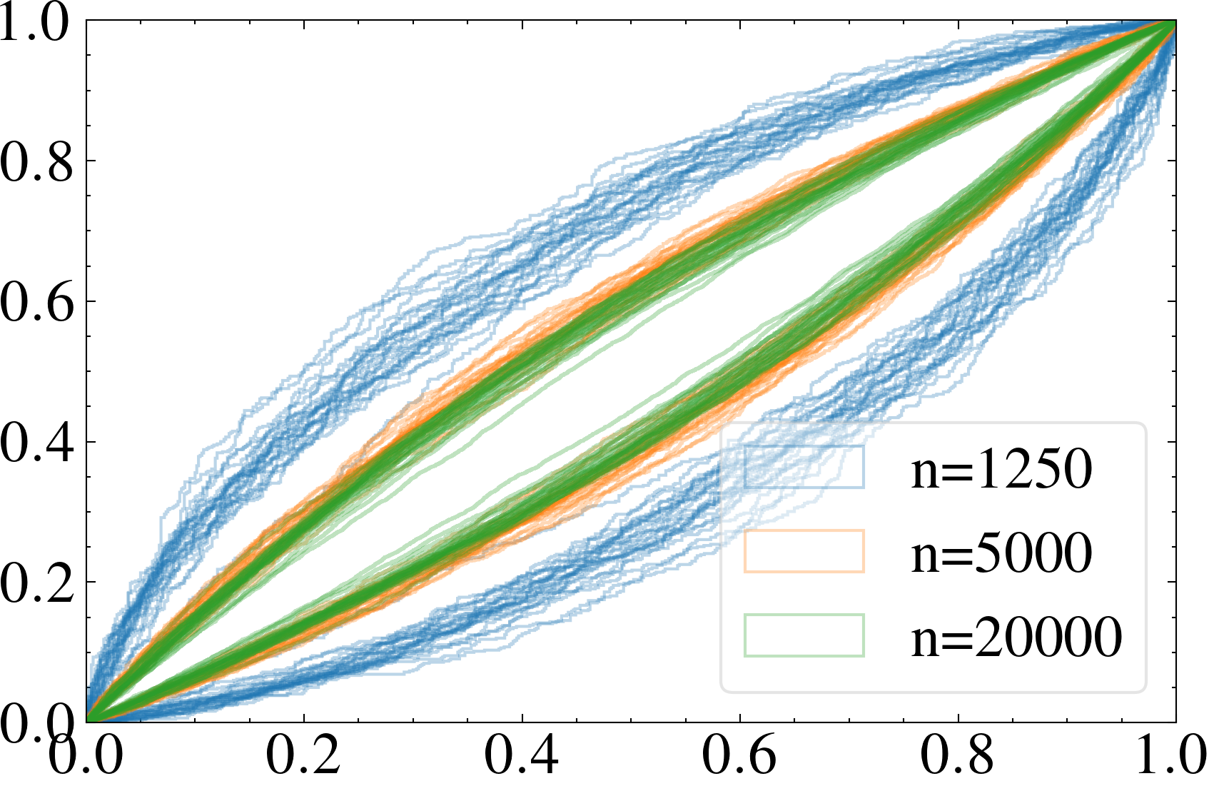
(a)

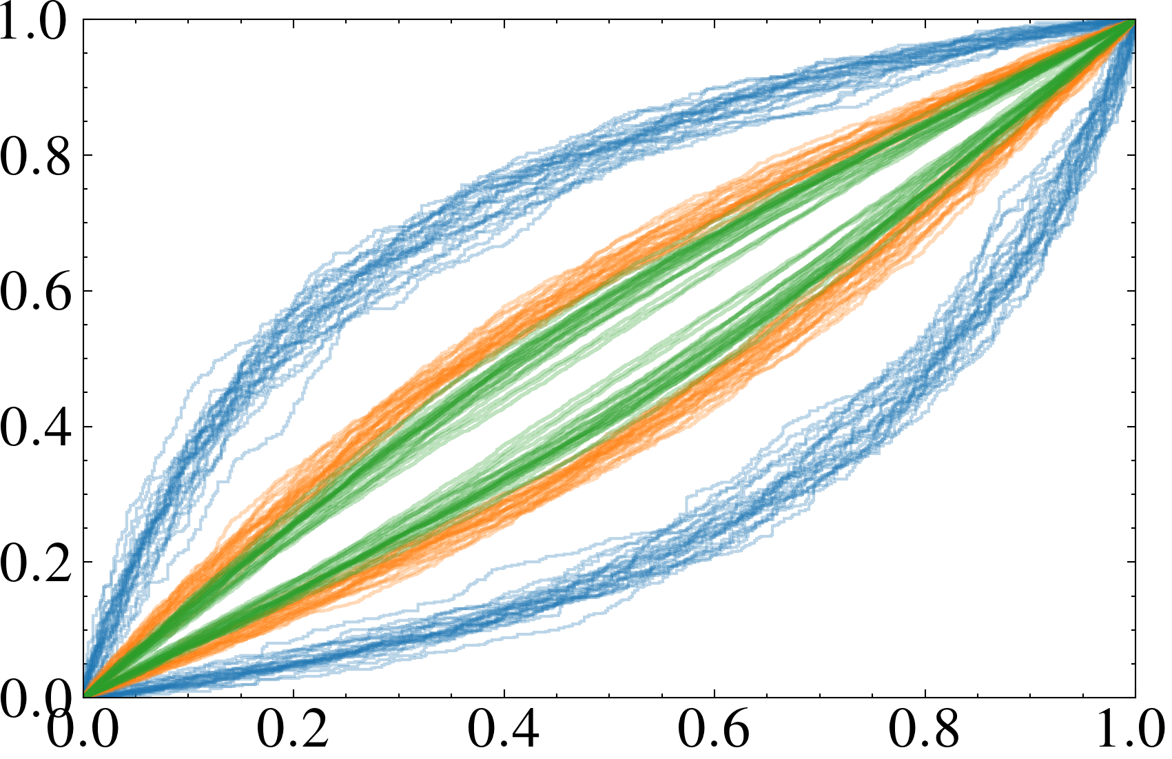
(b)

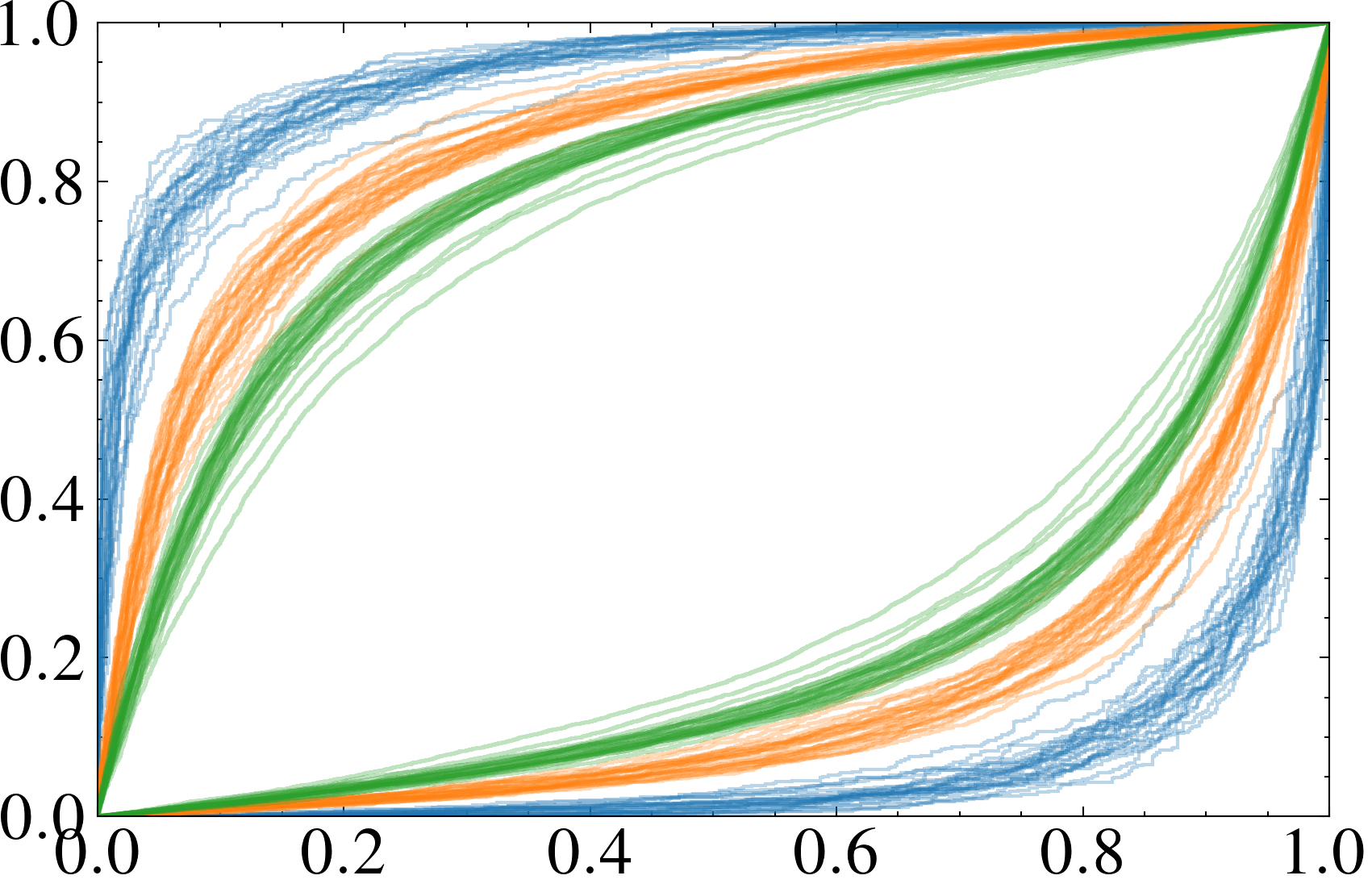
(c)

Figure 5: Visualization of the achievable region corresponding to the recognizability of representations on three datasets with varying training set sizes. Each polygon represents one run of the experiment. Smaller polygons indicate less recognizability.

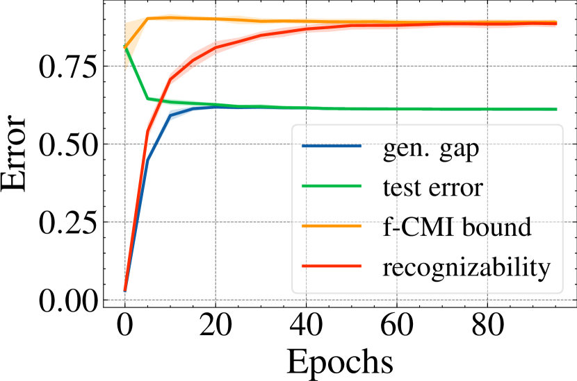
Figure 6: Dynamics of recognizability on CIFAR10 with size $n=1250$.

4.2.3   Impacts of $\beta$

To investigate the impacts of the regularization term of the RIB objective, we train models using the RIB objective with various $\beta$. The results on SVHN and CIFAR10 are illustrated in Fig. 3. We can observe that: i) When training data is scarce, the model obtains the best performance at larger $\beta$. This is expected since the model tends to over-fit to the data in this case. ii) SVHN is more tolerant of large $\beta$ compared to CIFAR10. When increasing the $\beta$ to more than ${10}^{3}$, the model still outperforms the CE baseline in most cases, while too large $\beta$ may lead to instability in CIFAR10 training. We consider this because the features of SVHN are easier to learn than those of CIFAR10 and are more likely to be over-fitted to irrelevant features, thus regularization brings greater improvement. This provides us with some indications for choosing the best $\beta$ based on the characteristics of the dataset.

4.3 Estimation of Generalization Gap

To verify the recognizability of representations can be used to indicate the generalization performance, we conduct experiments on different training set sizes $n\in\{1250,5000,20000\}$ with the smaller dataset being a subset of the larger dataset. We first train the models on different dataset sizes respectively, and then train the recognizability critics using the representations obtained from the trained models on the smallest data subset respectively. This allows us to evaluate the generalization to the unseen samples outside the smallest subset. Each experiment is repeated $k_{1}k_{2}$ times to evaluate the f-CMI bound. As illustrated in Fig. 4, we find that i) both the recognizability of representations and the f-CMI bound reflect the generalization to the unseen data, and the recognizability of representations even obtains better estimates in some cases; ii) since the recognizability of representations is a parameterized approximation rather than an upper bound, the risk may sometimes be underestimated as in Fig. 4(b). We also visualize the achievable region corresponding to the recognizability of representations, which is obtained by plotting the ROC curve of the score function and its central symmetry about the point (1/2, 1/2). The symmetry of the achievable region is due to the fact that we can construct an opposite test when any test chooses $H_{0}$ it chooses $H_{1}$ and vice versa. The visualization results are illustrated in Fig. 6. We find that the better the generalization performance, the smaller the area of achievable regions, which validates the plausibility of our formulation. Since CIFAR10 features are more difficult to learn thus easier to over-fit, it can be seen that a larger area is covered than the other two datasets.

4.3.1   Recognizability Dynamics

To investigate how the recognizability changes during training, we evaluate the recognizability every 5 epochs and plot the dynamics of recognizability as the number of training epochs changes in Fig. 6. We observe that recognizability can track the generalization gap as expected and eventually converge to around the f-CMI bound. See Appendix C for more results.

5 Conclusions and Future Work

In this paper, we establish the connection between the recognizability of representations and the f-CMI bound, and propose the RIB to regularize the recognizability of representations through Bregman divergence. We conducted extensive experiments on several commonly used datasets to demonstrate the effectiveness of RIB in regularizing the model and estimating the generalization gap. Future work can investigate whether RIB is also effective on other tasks such as few-shot learning, out-of-distribution detection, domain generalization, etc.

Appendix A Proof of Theorem 1

We start with giving a formal definition of the ROC curve for log-likelihood ratio test (LRT). We consider two hypotheses, $H_{0}$ and $H_{1}$, corresponding to the detection of two distributions $P_{T|\tilde{Z}=\tilde{z}}$ and $P_{T|U,\tilde{Z}=\tilde{z}}$, respectively,

$$H_{0}:T\sim P_{T|\tilde{Z}=\tilde{z}}\qquad H_{1}:T\sim P_{T|U,\tilde{Z}=\tilde{z}}\,.$$

Denote $\xi(T)$ as the LRT statistic random variable w.r.t. $\xi$, while LRT is obtained by

$$\xi(t)=\log\frac{P_{T}(t|H_{1})}{P_{T}(t|H_{0})}=\log\frac{P_{T|U,\tilde{Z}=\tilde{z}}(t)}{P_{T|\tilde{Z}=\tilde{z}}(t)},$$

where $P_{T}(t|H_{0})$ and $P_{T}(t|H_{1})$ denote the distributions of $T$ under the hypothesis $H_{0}$ $H_{1}$, respectively. We also define $P_{0}(\tau)=\mathrm{Pr}(\xi(T)\geq\tau|H_{0})$ and $P_{1}(\tau)=\mathrm{Pr}(\xi(T)\geq\tau|H_{1})$, where $\tau$ is a threshold. Then, each point on the ROC curve can be achieved by $(P_{0}(\tau),P_{1}(\tau))$. Let $x=P_{0}(\tau)$, $P_{0}^{-1}$ be the inverse function of $P_{0}$, the ROC curve can be expressed as $\psi_{\xi}(x)=P_{1}(P_{0}^{-1}(x))$. For the sake of brevity, we omit the subscript $\xi$. Note that due to the properties of ROC, $\psi(x)$ is twice continuously differentiable on the interval $[0,1]$ and should satisfy the following conditions Levy (2008); Khajavi and Kuh (2018):

$$\int_{0}^{1}\psi^{\prime}(x)\,dx=1$$ (C1)

$$\psi^{\prime}(x)\geq 0$$ (C2)

$$\psi^{\prime\prime}(x)\leq 0$$ (C3)

We can express the area under the ROC curve by

$$\mathrm{AUCROC}_{\xi}=\int_{0}^{1}\psi(x)\,dx\,.$$

Our proof relies on the following lemma.

Lemma 2 (Lem. 1 of Khajavi and Kuh (2018)).

Let $\xi_{0}:=\xi(T)|H_{0}$, $\xi_{1}:=\xi(T)|H_{1}$, $P_{\xi_{0}}(t)$ and $P_{\xi_{1}}(t)$ be the distribution of the random variables $\xi_{0}$ and $\xi_{1}$, respectively. Given the ROC curve, $\psi(x)$, we can compute the Kullback-Leibler (KL) divergence

$$D_{\mathrm{KL}}(P_{\xi_{1}}(t)\|P_{\xi_{0}}(t))=-\int_{0}^{1}\log\psi^{\prime}(x)\,dx\,.$$ (10)

This lemma establishes the relationship between receiver operating characteristic (ROC) curves and KL divergence. We will use it to connect the recognizability of representations and the KL divergence.

Proof of Theorem 1.

We have that

$$D_{\mathrm{KL}}(P_{\xi_{1}}(t)\|P_{\xi_{0}}(t)) \leq D_{\mathrm{KL}}(P_{T}(t|H_{1})\|P_{T}(t|H_{0}))$$

$$=D_{\mathrm{KL}}(P_{T|U,\tilde{Z}=\tilde{z}}(t)\|P_{T|\tilde{Z}=\tilde{z}}(t)),$$

where the inequality holds by the data processing property for divergences Polyanskiy and Wu (2019) and the equation holds by definition. Now we can prove that the theorem holds by proving the following inequality

$$\Re(P_{T|\tilde{Z}=\tilde{z}},P_{T|U,\tilde{Z}=\tilde{z}})\leq D_{\mathrm{KL}}(P_{\xi_{1}}(t)\|P_{\xi_{0}}(t))+\log\frac{e}{2}\,.$$ (11)

By definition, we have that

$$\Re(P_{T|\tilde{Z}=\tilde{z}},P_{T|U,\tilde{Z}=\tilde{z}})=2\int_{0}^{1}\psi(x)\,dx-1\,.$$ (12)

Using integration by parts, we have $\int_{0}^{1}\psi(x)\,dx=1-\int_{0}^{1}x\psi^{\prime}(x)\,dx$. Substituting this into Eq. 12 gives

$$\Re(P_{T|\tilde{Z}=\tilde{z}},P_{T|U,\tilde{Z}=\tilde{z}})=1-2\int_{0}^{1}x\psi^{\prime}(x)\,dx\,.$$ (13)

Substituting Eqs. 10 and 13 into Inequality (11) and rearranging terms yields the following new goal:

$$\int_{0}^{1}2x\psi^{\prime}(x)-\log\psi^{\prime}(x)\,dx\geq\log 2\,.$$ (14)

Next we will prove that the minimum of the LHS of Inequality (14) is greater than $\log 2$. We convert the proof into an optimization problem as follows

$$\begin{gathered}\arg\min_{\psi^{\prime}(x)}\int_{0}^{1}2x\psi^{\prime}(x)-\log\psi^{\prime}(x)\,dx\\ \text{s.t. (\ref{eq:cond1})-(\ref{eq:cond3})}\,.\end{gathered}$$ (15)

We then express Eq. 15 with a Lagrangian multiplier $\lambda>0$ and yields the following Lagrangian

$$L(\psi^{\prime}(x),\lambda)=\int_{0}^{1}2x\psi^{\prime}(x)-\log\psi^{\prime}(x)\,dx+\lambda(\int_{0}^{1}\psi^{\prime}(x)\,dx-1)\,.$$

Since the Lagrangian $L(\psi^{\prime}(x),\lambda)$ is a convex functional of $\psi^{\prime}(x)$, we can now calculate its derivative w.r.t. $\psi^{\prime}(x)$ by

$$\frac{\partial L(\psi^{\prime}(x),\lambda)}{\partial\psi^{\prime}(x)}=\int_{0}^{1}(2x-\frac{1}{\psi^{\prime}(x)}+\lambda)\,dx\,.$$

Setting $\frac{\partial L(\psi^{\prime}(x),\lambda)}{\partial\psi^{\prime}(x)}=0$, we obtain

$$\psi^{\prime}(x)=\frac{1}{2x+\lambda}\,.$$ (16)

Substituting Eq. 16 into Inequality (14) and calculating the definite integral gives

$$\int_{0}^{1}\frac{2x}{2x+\lambda}+\log(2x+\lambda)\,dx=\log(2+\lambda)\geq\log 2,$$

which concludes the proof of the theorem. ∎

Appendix B Additional Experimental Details

B.1 Network Architectures

In this work, we employ two deep models: a neural network encoder to learn the representations and a recognizability critic to learn the recognizability of representations. The specific network architectures are presented in Tables 3 and 4, respectively.

Type	Parameters
Conv	128 filters, $4\times 4$ kernels, stride 2, padding 1, batch normalization, ReLU
Conv	128 filters, $4\times 4$ kernels, stride 2, padding 1, batch normalization, ReLU
Conv	256 filters, $3\times 3$ kernels, stride 2, padding 0, batch normalization, ReLU
Conv	1024 filters, $3\times 3$ kernels, stride 1, padding 0, batch normalization, ReLU
FC	1024 units, ReLU
FC	512 units, ReLU

Table 3: The network architecture of the neural network encoder.

Type	Parameters
FC	1024 units, LeakyReLU
FC	1024 units, LeakyReLU
FC	1024 units, LeakyReLU
FC	1 unit, linear activation

Table 4: The network architecture of the recognizability critic.

B.2 Training Set Sizes

We set three data scales analogous to Harutyunyan et al. (2021) but with some minor changes. For MNIST, Fashion-MNIST, SVHN and CIFAR10, we set the training set sizes to $\{1250,5000,20000\}$, the smaller one is a quarter of the larger one; for STL10, we set the training set sizes to $\{625,1250,2500\}$, since it contains only 5000 training samples and we should keep at least half of them to form a ghost set.

Appendix C Additional Experimental Results

C.1 Density-ratio Matching Using Different Measures

The Bregman divergence is a generalized measure of the difference between two points. Applying different $F(R)$ will degrade the Bregman divergence to correspondingly different measures. Several choices of $F(R)$ commonly used in density-ratio matching Sugiyama et al. (2012) are given in Table 5. Table 6 shows that they do not exhibit significant performance differences.

Name	$F(R)$	$D_{\mathrm{BR}}(R^{*}\|R)$
Binary KL (BKL) divergence	$R\log R-(1+R)\log(1+R)$	$(1+R)\log\frac{1+R}{1+R^{*}}+R^{*}\log\frac{R^{*}}{R}$
Squared (SQ) distance	$(R-1)^{2}/2$	$\frac{1}{2}(R^{*}-R)^{2}$
Unnormalized KL (UKL) divergence	$R\log R-R$	$R^{*}\log\frac{R^{*}}{R}-R^{*}+R$

Table 5: Summary of density ratio matching using different measures.

Method	Fashion			SVHN			CIFAR10
	1250	5000	20000	1250	5000	20000	1250	5000	20000
RIB	17.05±0.41	13.57±0.28	9.32±0.25	27.72±1.17	17.37±0.52	10.80±0.27	59.16±1.17	47.57±0.60	31.06±0.38
RIBSQ	17.06±0.51	13.63±0.34	9.46±0.24	28.26±1.05	17.19±0.44	10.74±0.23	59.46±1.03	47.20±1.07	31.33±0.41
RIBUKL	17.06±0.39	13.51±0.39	9.40±0.27	28.14±1.27	17.20±0.38	10.80±0.32	59.57±1.02	47.15±0.60	31.13±0.50

Table 6: Comparison of the mean test error (%) on three datasets with different measure function as Bregman divergence.

C.2 Regularization Effects on MNIST and STL10

We report additional results on MNIST and STL10 that are not included in the main text due to space constraints. Table 7 shows that RIB still outperforms other baselines across all datasets and all training set sizes. This again demonstrates that the effectiveness of the RIB objective in improving the generalization performance of the model.

Method	MNIST			STL10
	1250	5000	20000	625	1250	2500
CE	4.75±1.00	2.43±0.29	1.00±0.09	66.62±1.20	61.88±1.01	56.21±0.97
L2	4.25±0.39	2.46±0.26	0.95±0.19	66.47±0.71	62.26±1.50	56.77±1.38
Dropout	4.58±0.40	2.47±0.21	1.01±0.13	66.58±0.98	61.77±0.86	56.53±0.92
VIB	3.64±0.20	1.98±0.13	0.87±0.07	63.69±1.11	59.76±0.95	54.73±0.67
NIB	4.29±0.27	2.34±0.18	0.95±0.07	66.16±0.72	61.49±0.99	55.71±0.64
DIB	3.86±0.45	1.97±0.12	0.86±0.06	66.20±0.75	61.43±0.94	55.63±0.71
PIB	4.35±0.24	2.29±0.17	0.96±0.08	66.16±0.97	61.59±0.63	55.93±0.53
RIB	3.47±0.29	1.82±0.12	0.85±0.08	62.88±0.81	58.99±1.04	54.34±0.77

Table 7: Comparison of the mean test error (%) on MNIST and STL10 with different training set sizes.

C.3 Estimation of Generalization Gap on MNIST and STL10

We verify that the recognizability of representations is able to indicate the generalization to unseen data on MNIST and STL10. As illustrated in Fig. 7, the recognizability curves are still able to keep track of the generalization gaps as well as the f-CMI bounds. The visualization results of the achievable region corresponding to the recognizability of representations are illustrated in Fig. 8. We can still find that the better the generalization performance, the smaller the area of achievable regions, and the area corresponding to MNIST is significantly smaller than that of STL10 since the former is much easier to learn, while the latter has fewer samples making the model prone to over-fitting.

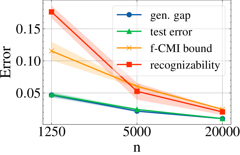
(a) MNIST

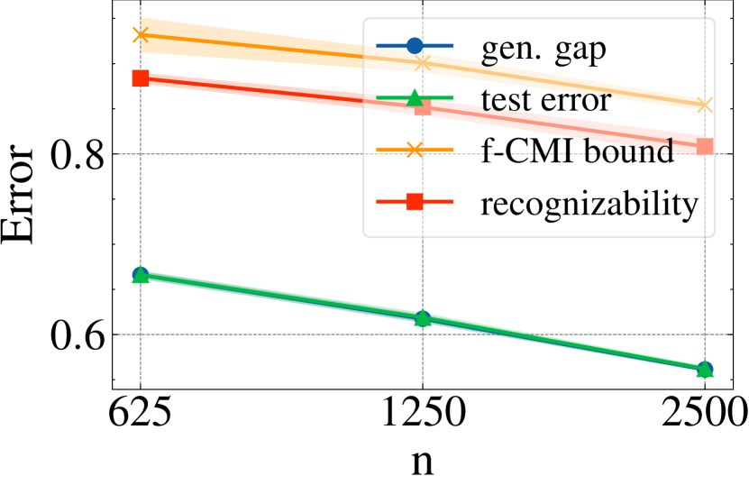
(b) STL10

Figure 7: Comparison of expected generalization gap, mean test error, f-CMI bound and recognizability of representations on MNIST and STL10 with varying training set sizes.

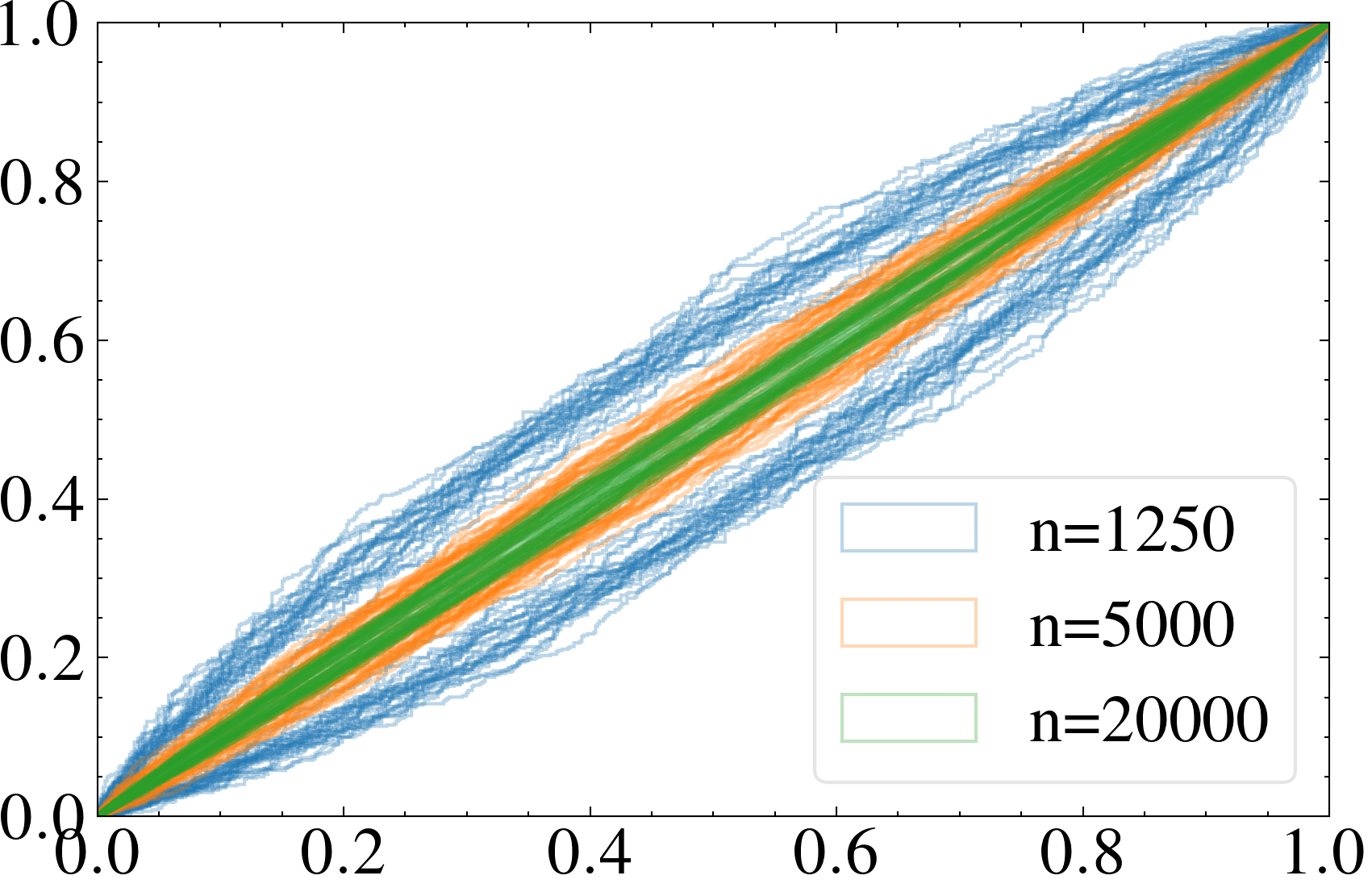
(a) MNIST

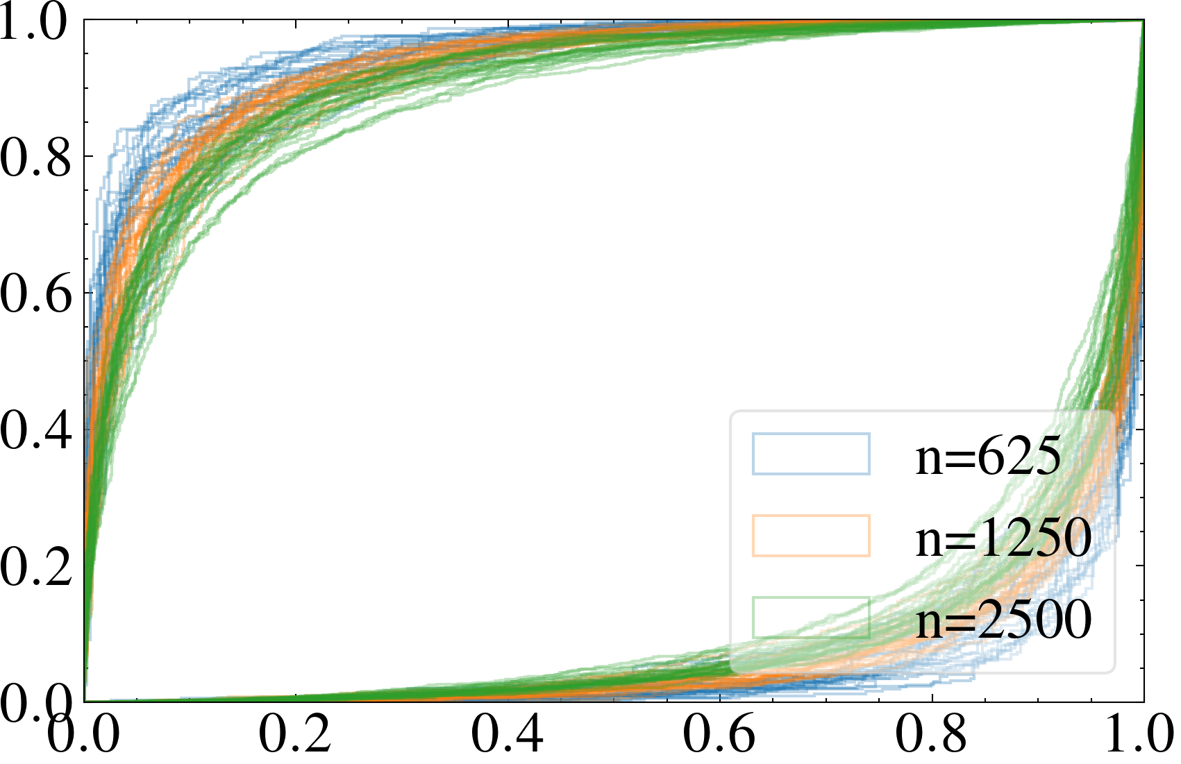
(b) STL10

Figure 8: Visualization of the achievable region corresponding to the recognizability of representations on MNIST and STL10 with varying training set sizes. Each polygon represents one run of the experiment. Smaller polygons indicate less recognizability.

C.4 Recognizability Dynamics

We report the dynamics of recognizability on CIFAR10 with training set sizes of 5000 and 20000 in Fig. 9.

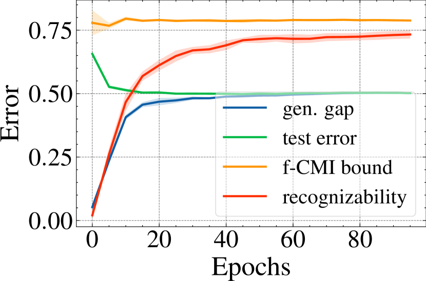
(a) $n=5000$

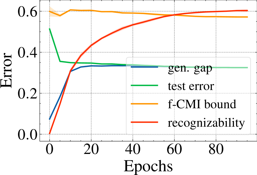
(b) $n=20000$

Figure 9: Dynamics of recognizability on CIFAR10 with training set sizes of 5000 and 20000.

Appendix D Computational Complexity Analysis

Table 8 presents our computational complexity analysis, where $m$ is the number of data points, $d$ and $d^{\prime}$ are the dimension of the encoder network and the recognizability critic, respectively, and $c$ is the number of iterations used to estimate the Fisher information matrix. Note that the raw PIB objective requires a number of approximations to make the computational complexity affordable, due to the use of second-order information. Nevertheless, the computational complexity of the PIB is still higher than that of the RIB.

SGD PIB (w/o approx.) PIB RIB $\mathcal{O}(md)$ $\mathcal{O}(md+md^{2})$ $\mathcal{O}(md+cmd)$ $\mathcal{O}(md+md^{\prime})$

Table 8: Comparison of computational complexity per step.

References

- Alemi et al. [2017] Alexander A. Alemi, Ian Fischer, Joshua V. Dillon, and Kevin Murphy. Deep variational information bottleneck. In 5th International Conference on Learning Representations, ICLR 2017, Toulon, France, April 24-26, 2017, Conference Track Proceedings. OpenReview.net, 2017.
- Banerjee and Montúfar [2021] Pradeep Kr. Banerjee and Guido Montúfar. Information complexity and generalization bounds. In IEEE International Symposium on Information Theory, ISIT 2021, Melbourne, Australia, July 12-20, 2021, pages 676–681. IEEE, 2021.
- Bu et al. [2020] Yuheng Bu, Shaofeng Zou, and Venugopal V. Veeravalli. Tightening mutual information-based bounds on generalization error. IEEE J. Sel. Areas Inf. Theory, 1(1):121–130, 2020.
- Catoni [2007] Olivier Catoni. Pac-bayesian supervised classification: The thermodynamics of statistical learning. IMS Lecture Notes Monograph Series, 56:1–163, 2007. arXiv:0712.0248 [stat].
- Coates et al. [2011] Adam Coates, Andrew Y. Ng, and Honglak Lee. An analysis of single-layer networks in unsupervised feature learning. In Geoffrey J. Gordon, David B. Dunson, and Miroslav Dudík, editors, Proceedings of the Fourteenth International Conference on Artificial Intelligence and Statistics, AISTATS 2011, Fort Lauderdale, USA, April 11-13, 2011, volume 15, pages 215–223. JMLR.org, 2011.
- Du et al. [2020] Ying-Jun Du, Jun Xu, Huan Xiong, Qiang Qiu, Xiantong Zhen, Cees G. M. Snoek, and Ling Shao. Learning to learn with variational information bottleneck for domain generalization. In Computer Vision - ECCV 2020 - 16th European Conference, Glasgow, UK, August 23-28, 2020, Proceedings, Part X, volume 12355, pages 200–216. Springer, 2020.
- Dubois et al. [2020] Yann Dubois, Douwe Kiela, David J. Schwab, and Ramakrishna Vedantam. Learning optimal representations with the decodable information bottleneck. In NeurIPS 2020, December 6-12, 2020, virtual, 2020.
- Dziugaite and Roy [2017] Gintare Karolina Dziugaite and Daniel M. Roy. Computing nonvacuous generalization bounds for deep (stochastic) neural networks with many more parameters than training data. In Proceedings of the Thirty-Third Conference on Uncertainty in Artificial Intelligence, UAI 2017, Sydney, Australia, August 11-15, 2017. AUAI Press, 2017.
- Gálvez et al. [2020] Borja Rodríguez Gálvez, Ragnar Thobaben, and Mikael Skoglund. The convex information bottleneck lagrangian. Entropy, 22(1):98, 2020.
- Goodfellow et al. [2014] Ian J. Goodfellow, Jean Pouget-Abadie, Mehdi Mirza, Bing Xu, David Warde-Farley, Sherjil Ozair, Aaron C. Courville, and Yoshua Bengio. Generative adversarial nets. In NeurIPS 2014, December 8-13 2014, Montreal, Quebec, Canada, pages 2672–2680, 2014.
- Haghifam et al. [2020] Mahdi Haghifam, Jeffrey Negrea, Ashish Khisti, Daniel M. Roy, and Gintare Karolina Dziugaite. Sharpened generalization bounds based on conditional mutual information and an application to noisy, iterative algorithms. In NeurIPS 2020, December 6-12, 2020, virtual, 2020.
- Harutyunyan et al. [2021] Hrayr Harutyunyan, Maxim Raginsky, Greg Ver Steeg, and Aram Galstyan. Information-theoretic generalization bounds for black-box learning algorithms. In NeurIPS 2021, December 6-14, 2021, virtual, pages 24670–24682, 2021.
- Hjelm et al. [2019] R. Devon Hjelm, Alex Fedorov, Samuel Lavoie-Marchildon, Karan Grewal, Philip Bachman, Adam Trischler, and Yoshua Bengio. Learning deep representations by mutual information estimation and maximization. In 7th International Conference on Learning Representations, ICLR 2019, New Orleans, LA, USA, May 6-9, 2019. OpenReview.net, 2019.
- Khajavi and Kuh [2018] Navid Tafaghodi Khajavi and Anthony Kuh. Covariance selection quality through detection problem and auc bounds. APSIPA Transactions on Signal and Information Processing, 7:e19, 2018.
- Kingma and Ba [2015] Diederik P. Kingma and Jimmy Ba. Adam: A method for stochastic optimization. In 3rd International Conference on Learning Representations, ICLR 2015, San Diego, CA, USA, May 7-9, 2015, Conference Track Proceedings, 2015.
- Kolchinsky et al. [2019] Artemy Kolchinsky, Brendan D. Tracey, and David H. Wolpert. Nonlinear information bottleneck. Entropy, 21(12):1181, 2019.
- Krizhevsky et al. [2009] Alex Krizhevsky, Geoffrey Hinton, et al. Learning multiple layers of features from tiny images. 2009.
- Lai et al. [2021] Qiuxia Lai, Yu Li, Ailing Zeng, Minhao Liu, Hanqiu Sun, and Qiang Xu. Information bottleneck approach to spatial attention learning. In Proceedings of the Thirtieth International Joint Conference on Artificial Intelligence, IJCAI 2021, Virtual Event / Montreal, Canada, 19-27 August 2021, pages 779–785. ijcai.org, 2021.
- Levy [2008] Bernard C. Levy. Binary and M-ary Hypothesis Testing, page 1–57. Springer US, Boston, MA, 2008.
- Li et al. [2022] Bo Li, Yifei Shen, Yezhen Wang, Wenzhen Zhu, Colorado Reed, Dongsheng Li, Kurt Keutzer, and Han Zhao. Invariant information bottleneck for domain generalization. In Thirty-Sixth AAAI Conference on Artificial Intelligence, Virtual Event, February 22 - March 1, 2022, pages 7399–7407. AAAI Press, 2022.
- Negrea et al. [2019] Jeffrey Negrea, Mahdi Haghifam, Gintare Karolina Dziugaite, Ashish Khisti, and Daniel M. Roy. Information-theoretic generalization bounds for SGLD via data-dependent estimates. In NeurIPS 2019, December 8-14, 2019, Vancouver, BC, Canada, pages 11013–11023, 2019.
- Netzer et al. [2011] Yuval Netzer, Tao Wang, Adam Coates, Alessandro Bissacco, Bo Wu, and Andrew Y. Ng. Reading digits in natural images with unsupervised feature learning. In NIPS Workshop on Deep Learning and Unsupervised Feature Learning 2011, 2011.
- Neyman et al. [1933] Jerzy Neyman, Egon Sharpe Pearson, and Karl Pearson. On the problem of the most efficient tests of statistical hypotheses. Philosophical Transactions of the Royal Society of London. Series A, Containing Papers of a Mathematical or Physical Character, 231(694–706):289–337, Feb 1933.
- Nowozin et al. [2016] Sebastian Nowozin, Botond Cseke, and Ryota Tomioka. f-gan: Training generative neural samplers using variational divergence minimization. In NeurIPS 2016, December 5-10, 2016, Barcelona, Spain, pages 271–279, 2016.
- Pan et al. [2021] Ziqi Pan, Li Niu, Jianfu Zhang, and Liqing Zhang. Disentangled information bottleneck. In Thirty-Fifth AAAI Conference on Artificial Intelligence, AAAI 2021, Virtual Event, February 2-9, 2021, pages 9285–9293. AAAI Press, 2021.
- Pensia et al. [2018] Ankit Pensia, Varun S. Jog, and Po-Ling Loh. Generalization error bounds for noisy, iterative algorithms. In 2018 IEEE International Symposium on Information Theory, ISIT 2018, Vail, CO, USA, June 17-22, 2018, pages 546–550. IEEE, 2018.
- Polyanskiy and Wu [2019] Yury Polyanskiy and Yihong Wu. Lecture notes on information theory. Technical report, 2019.
- Poole et al. [2019] Ben Poole, Sherjil Ozair, Aäron van den Oord, Alexander A. Alemi, and George Tucker. On variational bounds of mutual information. In Proceedings of the 36th International Conference on Machine Learning, ICML 2019, 9-15 June 2019, Long Beach, California, USA, volume 97, pages 5171–5180. PMLR, 2019.
- Rodriguez Galvez [2019] Borja Rodriguez Galvez. The information bottleneck : Connections to other problems, learning and exploration of the ib curve. Master’s thesis, KTH, School of Electrical Engineering and Computer Science (EECS), 2019.
- Saxe et al. [2018] Andrew M. Saxe, Yamini Bansal, Joel Dapello, Madhu Advani, Artemy Kolchinsky, Brendan D. Tracey, and David D. Cox. On the information bottleneck theory of deep learning. In 6th International Conference on Learning Representations, ICLR 2018, Vancouver, BC, Canada, April 30 - May 3, 2018, Conference Track Proceedings. OpenReview.net, 2018.
- Shamir et al. [2010] Ohad Shamir, Sivan Sabato, and Naftali Tishby. Learning and generalization with the information bottleneck. Theor. Comput. Sci., 411(29-30):2696–2711, 2010.
- Srivastava et al. [2014] Nitish Srivastava, Geoffrey E. Hinton, Alex Krizhevsky, Ilya Sutskever, and Ruslan Salakhutdinov. Dropout: a simple way to prevent neural networks from overfitting. J. Mach. Learn. Res., 15(1):1929–1958, 2014.
- Steinke and Zakynthinou [2020] Thomas Steinke and Lydia Zakynthinou. Reasoning about generalization via conditional mutual information. In Conference on Learning Theory, COLT 2020, 9-12 July 2020, Virtual Event [Graz, Austria], volume 125, pages 3437–3452. PMLR, 2020.
- Sugiyama et al. [2012] Masashi Sugiyama, Taiji Suzuki, and Takafumi Kanamori. Density-ratio matching under the bregman divergence: a unified framework of density-ratio estimation. Annals of the Institute of Statistical Mathematics, 64(5):1009–1044, Oct 2012.
- Tishby et al. [2000] Naftali Tishby, Fernando C. N. Pereira, and William Bialek. The information bottleneck method. CoRR, physics/0004057, 2000.
- Vera et al. [2018] Matías Vera, Pablo Piantanida, and Leonardo Rey Vega. The role of the information bottleneck in representation learning. In 2018 IEEE International Symposium on Information Theory, ISIT 2018, Vail, CO, USA, June 17-22, 2018, pages 1580–1584. IEEE, 2018.
- Wang et al. [2022] Zifeng Wang, Shao-Lun Huang, Ercan Engin Kuruoglu, Jimeng Sun, Xi Chen, and Yefeng Zheng. PAC-bayes information bottleneck. In International Conference on Learning Representations, 2022.
- Xiao et al. [2017] Han Xiao, Kashif Rasul, and Roland Vollgraf. Fashion-mnist: a novel image dataset for benchmarking machine learning algorithms. CoRR, abs/1708.07747, 2017.
- Xu and Raginsky [2017] Aolin Xu and Maxim Raginsky. Information-theoretic analysis of generalization capability of learning algorithms. In NeurIPS 2017, December 4-9, 2017, Long Beach, CA, USA, pages 2524–2533, 2017.
- Yu et al. [2021] Xi Yu, Shujian Yu, and José C. Príncipe. Deep deterministic information bottleneck with matrix-based entropy functional. In IEEE International Conference on Acoustics, Speech and Signal Processing, ICASSP 2021, Toronto, ON, Canada, June 6-11, 2021, pages 3160–3164. IEEE, 2021.
- Zhou et al. [2022] Ruida Zhou, Chao Tian, and Tie Liu. Individually conditional individual mutual information bound on generalization error. IEEE Trans. Inf. Theory, 68(5):3304–3316, 2022.