A gauge constrained algorithm of VDAT at $\mathcal{N}=3$ for the multi-orbital Hubbard model

Abstract

The recently developed variational discrete action theory (VDAT) provides a systematic variational approach to the ground state of the quantum many-body problem, where the quality of the solution is controlled by an integer $\mathcal{N}$, and increasing $\mathcal{N}$ monotonically approaches the exact solution. VDAT can be exactly evaluated in the $d=\infty$ multi-orbital Hubbard model using the self-consistent canonical discrete action theory (SCDA), which requires a self-consistency condition for the integer time Green’s functions. Previous work demonstrates that $\mathcal{N}=3$ accurately captures multi-orbital Mott/Hund physics at a cost similar to the Gutzwiller approximation. Here we employ a gauge constraint to automatically satisfy the self-consistency condition of the SCDA at $\mathcal{N}=3$, yielding an even more efficient algorithm with enhanced numerical stability. We derive closed form expressions of the gauge constrained algorithm for the multi-orbital Hubbard model with general density-density interactions, allowing VDAT at $\mathcal{N}=3$ to be straightforwardly applied to the seven orbital Hubbard model. We present results and a performance analysis using $\mathcal{N}=2$ and $\mathcal{N}=3$ for the $\textrm{SU}(2\textrm{N}_{\textrm{orb}})$ Hubbard model in $d=\infty$ with $\textrm{N}_{\textrm{orb}}=2-8$, and compare to numerically exact dynamical mean-field theory solutions where available. The developments in this work will greatly facilitate the application of VDAT at $\mathcal{N}=3$ to strongly correlated electron materials.

I Introduction

The recently developed variational discrete action theory (VDAT) [5, 6] has emerged as a powerful tool to study the ground state of the multi-orbital Hubbard model [4], which can be considered as a minimal model for a wide class of strongly correlated electron materials [15, 17]. VDAT consists of two central components: the sequential product density matrix (SPD) ansatz and the discrete action theory to evaluate observables under the SPD. The accuracy of the SPD is controlled by an integer $\mathcal{N}$, and the SPD monotonically approaches the exact solution for increasing $\mathcal{N}$. In the context of the Hubbard model, the SPD recovers most well known variational wavefunctions [5]: $\mathcal{N}=1$ recovers the Hartree-Fock wave function, $\mathcal{N}=2$ recovers the Gutzwiller wave function [11, 12, 13], and $\mathcal{N}=3$ recovers the Gutzwiller-Baeriswyl [22] and Baeriswyl-Gutzwiller wavefunctions [8]. The discrete action theory can be viewed as an integer time generalization of the imaginary time path integral, yielding an integer time generalization of the Green’s function and Dyson equation [5]. For $d=\infty$, the SPD can be exactly evaluated using the self-consistent canonical discrete action (SCDA) [5, 6]. VDAT within the SCDA offers a paradigm shift away from the dynamical mean-field theory (DMFT) [10, 17, 29], allowing the exact solution of the ground state properties of the $d=\infty$ Hubbard model to be systematically approached within the wave function paradigm. The computational cost of VDAT grows with $\mathcal{N}$, at an exponential scaling for an exact evaluation and a polynomial scaling for a numerical evaluation using Monte-Carlo, so rapid convergence with $\mathcal{N}$ is important if VDAT is to be a practical alternative to DMFT. VDAT using $\mathcal{N}=2,3,4$ has been applied to the single orbital Anderson impurity model on a ring [6], the $d=\infty$ single orbital Hubbard model [6], and the $d=\infty$ two orbital Hubbard model [4], and in all cases $\mathcal{N}=3$ yields accurate results as compared to the numerically exact solutions. This success is particularly nontrivial in the two orbital problem, where complex local interactions including the Hubbard $U$, Hund $J$, and crystal field $\Delta$ were studied over all parameter space. Therefore, VDAT within the SCDA at $\mathcal{N}=3$ provides a minimal and accurate description of the two orbital Hubbard model, but with a computational cost that is comparable to $\mathcal{N}=2$, which recovers the Gutzwiller approximation [13] (GA) and slave boson mean-field theories [16, 3, 24]. The fact that VDAT within the SCDA at $\mathcal{N}=3$ resolves all the limitations of the Gutzwiller approximation and the slave boson mean-field theories without substantially increasing the computational cost motivates a deeper understanding of how the SCDA works.

The SCDA provides a route for exactly evaluating the SPD in $d=\infty$, and the SCDA can be viewed as the integer time analogue of DMFT [5, 4]. While DMFT maps the Hubbard model to a self-consistently determined Anderson impurity model, the SCDA maps the SPD to a self-consistently determined canonical discrete action (CDA), parametrized by the corresponding non-interacting integer time Green’s function $\mathcal{G}$, which implicitly depends on the variational parameters of the SPD. While the DMFT self-consistency condition only needs to be executed once, the SCDA self-consistency condition must be executed for every choice of variational parameters during the minimization. Previously, we proposed an approach to mitigate this issue by simultaneously minimizing the variational parameters and updating $\mathcal{G}$, and demonstrated it to be efficient for the two band Hubbard model [4]. However, for some regions of parameter space, such as in the large polarization regime, a very small step size is needed to maintain numerical stability. Such problems are partially due to inaccuracies of $\mathcal{G}$ within the iteration process, given that $\mathcal{G}$ is only highly precise when the fixed point is reached. Therefore, it would be advantageous if the self-consistency condition of the SCDA could be automatically satisfied.

Given that $\mathcal{N}=2$ recovers the GA, it is interesting to recall how the GA automatically satisfies the SCDA self-consistency condition. As previously demonstrated [5], the GA has a prescribed form of $\mathcal{G}$ which is fully determined by imposing that the non-interacting and interacting local single particle density matrices are identical, which we refer to as the Gutzwiller gauge. While the SCDA at $\mathcal{N}=2$ can evaluate an SPD with arbitrary variational parameters, the GA is only valid when the SPD satisfies the Gutzwiller gauge. Therefore, the GA is a special case of the SCDA at $\mathcal{N}=2$, but the Gutzwiller gauge does not limit the variational power of the SPD due to the gauge freedom of the SPD [4]. In summary, the GA provides an important lesson for numerically simplifying the SCDA at $\mathcal{N}=2$ by exploiting the gauge freedom of the SPD, converting the problem of solving for $\mathcal{G}$ into a constraint on the variational parameters of the SPD. In this paper, we demonstrate that the lessons of the GA can be generalized to $\mathcal{N}=3$, which quantitatively captures the Mott and Hund physics of the multi-orbital Hubbard model [4].

In order to demonstrate the power of the gauge constrained implementation of the SCDA at $\mathcal{N}=3$, we study the $\textrm{SU}(2\textrm{N}_{\textrm{orb}})$ Hubbard model in $d=\infty$ with $\textrm{N}_{\textrm{orb}}=2-8$. Our successful execution of these calculations demonstrates the viability of applying VDAT at $\mathcal{N}=3$ to crystals bearing $d$ or $f$ electrons. Moreover, the $\textrm{SU}(2\textrm{N}_{\textrm{orb}})$ Hubbard model is interesting in its own right, given that experiments on ultracold atoms in an optical lattice can realize the $\textrm{SU}(2\textrm{N}_{\textrm{orb}})$ Hubbard model[27, 14, 23, 26, 25, 30]. Therefore, VDAT should serve as a reliable tool for understanding and interpreting such experimental measurements.

The structure of this paper is as follows. Sec. II presents the gauge constrained algorithm of the SCDA at $\mathcal{N}=3$, with Sec. II.1 providing a high level overview of the entire algorithm, including all key equations, while the remaining subsections provide detailed derivations. Sec. III presents results for the $\textrm{SU}(2\textrm{N}_{\textrm{orb}})$ Hubbard model in $d=\infty$ with $\textrm{N}_{\textrm{orb}}=2-8$.

II Gauge constrained algorithm at $\mathcal{N}$=3

II.1 Overview

The goal of this subsection is to provide an overview of the gauge constrained algorithm for the SCDA at $\mathcal{N}=3$, and Secs. II.2, II.3, and II.4 will derive all details of the procedure. We begin by highlighting how the SCDA exactly evaluates the SPD in $d=\infty$ [5, 6, 4]. Consider a fermionic lattice model having a Hamiltonian

$$\hat{H}=\hat{K}+\hat{H}_{loc}=\sum_{k\alpha\sigma}\epsilon_{k\alpha\sigma}\hat{n}_{k\alpha\sigma}+\sum_{i}\hat{H}_{loc;i},$$ (1)

where $i=1,\dots,\textrm{N}_{\textrm{site}}$ enumerates over the lattice sites, $k=1,\dots,\textrm{N}_{\textrm{site}}$ enumerates over the $k$-points, $\alpha=1,\dots,\textrm{N}_{\textrm{orb}}$ enumerates over the orbitals, and $\sigma$ enumerates over spin. The G-type SPD for $\mathcal{N}=3$ can be motivated from the following variational wave function

$$\exp\left(\sum_{k\alpha\sigma}\gamma_{k\alpha\sigma}\hat{n}_{k\alpha\sigma}\right)\prod_{i}\hat{P}_{i}\left(u\right)|\Psi_{0}\rangle,$$ (2)

where $\{\gamma_{k\alpha\sigma}\}$ is the set of non-interacting variational parameters, $u=\{u_{i\Gamma}\}$ is the set of interacting variational parameters, $\hat{P}_{i}\left(u\right)=\sum_{\Gamma}u_{i\Gamma}\hat{P}_{i\Gamma}$, and $|\Psi_{0}\rangle$ is a non-interacting variational wavefunction; and both $\{\gamma_{k\alpha\sigma}\}$ and $\{u_{i\Gamma}\}$ are real numbers. The index $\Gamma$ enumerates a set of many-body operators $\{\hat{P}_{i\Gamma}\}$ local to site $i$. The $\{\hat{P}_{i\Gamma}\}$ used for an $\hat{H}_{loc;i}$ containing only density-density type interactions is given in Eq. 34, while the general case is given in Eq. 134. It will be important to rewrite the above wave function as a density matrix, yielding the G-type SPD [5] for $\mathcal{N}=3$

$$\hat{\varrho} =\hat{\mathcal{P}}_{1}\hat{\mathcal{P}}_{2}\hat{\mathcal{P}}_{3}=\left(\hat{K}_{1}\hat{P}_{1}\right)\left(\hat{K}_{2}\hat{P}_{1}\right)\left(\hat{K}_{1}\right),$$ (3)

where $\hat{K}_{1}=\exp\left(\sum_{k\alpha\sigma}\gamma_{k\alpha\sigma}\hat{n}_{k\alpha\sigma}\right)$, $\hat{P}_{1}=\prod_{i}\hat{P}_{i}\left(u\right)$, and $\hat{K}_{2}=|\Psi_{0}\rangle\langle\Psi_{0}|$. Here we have chosen $\hat{K}_{1}$ to be diagonal in $k\alpha\sigma$, while the most general case is addressed in Ref. [4].

Evaluating expectation values under the SPD is highly nontrivial, and we have developed the discrete action theory [5] to formalize the problem in a manner which is amenable to systematic approximations. A key idea of the discrete action theory is the equivalence relation between an integer time correlation function and a corresponding expectation value in the compound space. An operator operator $\hat{O}$ in the original space is promoted to the compound space with a given integer time index $\tau$, denoted as $\textrm{\@text@baccent{$\hat{O}$}}^{(\tau)}$ [5]. For the total energy with $\mathcal{N}=3$, this equivalence is given as

$$\langle\hat{H}\rangle_{\hat{\varrho}} =\langle\textrm{\@text@baccent{$\hat{H}$}}^{\left(\mathcal{N}\right)}\rangle_{\textrm{\@text@baccent{$\hat{\spdsymb}$}}},$$ (4)

where $\textrm{\@text@baccent{$\hat{\spdsymb}$}}=\textrm{\@text@baccent{$\hat{\spdsymb}$}}_{0}\prod_{i}\textrm{\@text@baccent{$\hat{P}$}}_{i}$ is the discrete action of the SPD, $\textrm{\@text@baccent{$\hat{\spdsymb}$}}_{0}=\textrm{\@text@baccent{$\hat{Q}$}}\textrm{\@text@baccent{$\hat{K}$}}_{1}^{\left(1\right)}\textrm{\@text@baccent{$\hat{K}$}}_{2}^{\left(2\right)}\textrm{\@text@baccent{$\hat{K}$}}_{1}^{\left(3\right)}$ is the non-interacting discrete action, $̱\hat{Q}$ is the integer time translation operator [5, 4], and the interacting projector for site $i$ is

$$\textrm{\@text@baccent{$\hat{P}$}}_{i}=\textrm{\@text@baccent{$\hat{P}$}}_{i}^{\left(1\right)}(u)\textrm{\@text@baccent{$\hat{P}$}}_{i}^{\left(2\right)}(u)=\sum_{\Gamma\Gamma^{\prime}}u_{i\Gamma}u_{i\Gamma^{\prime}}\textrm{\@text@baccent{$\hat{P}$}}_{i\Gamma}^{\left(1\right)}\textrm{\@text@baccent{$\hat{P}$}}_{i\Gamma^{\prime}}^{\left(2\right)}.$$ (5)

An important previous result is that the expectation value in the compound space can be exactly evaluated for $d=\infty$ using the self-consistent canonical discrete action theory (SCDA) [6, 5].

Given the common scenario of translation symmetry, the SCDA can be presented in terms of two auxiliary effective discrete actions parameterized by $2\textrm{N}_{\text{orb}}\mathcal{N}\times 2\textrm{N}_{\text{orb}}\mathcal{N}$ matrices $\bm{S}_{loc}$ and $\bm{\mathcal{G}}$, given as

$$\langle\textrm{\@text@baccent{$\hat{H}$}}^{\left(\mathcal{N}\right)}\rangle_{\textrm{\@text@baccent{$\hat{\spdsymb}$}}}=\langle\textrm{\@text@baccent{$\hat{K}$}}^{\left(\mathcal{N}\right)}\rangle_{\textrm{\@text@baccent{$\hat{\rho}$}}_{K}}+\textrm{N}_{\textrm{site}}\langle\textrm{\@text@baccent{$\hat{H}$}}_{loc;i}^{\left(\mathcal{N}\right)}\rangle_{\textrm{\@text@baccent{$\hat{\rho}$}}_{loc;i}},$$ (6)

$$\textrm{\@text@baccent{$\hat{\rho}$}}_{K}=\textrm{\@text@baccent{$\hat{\spdsymb}$}}_{0}\exp\Big{(}-\sum_{i}\ln\bm{S}_{loc}^{T}\cdot\textrm{\@text@baccent{$\hat{\bm{n}}$}}_{i}\Big{)},$$ (7)

$$\textrm{\@text@baccent{$\hat{\rho}$}}_{loc;i}=\exp\Big{(}-\ln\left(\bm{\mathcal{G}}^{-1}-\boldsymbol{1}\right)^{T}\cdot\textrm{\@text@baccent{$\hat{\bm{n}}$}}_{i}\Big{)}\textrm{\@text@baccent{$\hat{P}$}}_{i},$$ (8)

where $[\textrm{\@text@baccent{$\hat{\bm{n}}$}}_{i}]_{\alpha\sigma\tau,\alpha^{\prime}\sigma^{\prime}\tau^{\prime}}=\textrm{\@text@baccent{$\hat{a}$}}_{i\alpha\sigma}^{\dagger(\tau)}\textrm{\@text@baccent{$\hat{a}$}}_{i\alpha^{\prime}\sigma^{\prime}}^{(\tau^{\prime})}$, the dot product operation is defined as $\boldsymbol{a}\cdot\hat{\boldsymbol{b}}\equiv\sum_{\ell\ell^{\prime}}[\boldsymbol{a}]_{\ell\ell^{\prime}}[\hat{\boldsymbol{b}}]_{\ell\ell^{\prime}}$, the discrete action $\textrm{\@text@baccent{$\hat{\rho}$}}_{K}$ is used to compute all single-particle integer time Green’s functions, and $\textrm{\@text@baccent{$\hat{\rho}$}}_{loc;i}$ is used to compute all N-particle integer time Green’s functions local to site $i$. The $\bm{\mathcal{G}}$ and $\bm{S}_{loc}$ must satisfy the following two self-consistency conditions

$$\left(\boldsymbol{g}_{loc}^{-1}-\boldsymbol{1}\right)=\left(\bm{\mathcal{G}}^{-1}-\boldsymbol{1}\right)\boldsymbol{S}_{loc},$$ (9)

$$\bm{g}_{loc}=\bm{g}^{\prime}_{loc},$$ (10)

where $\bm{g}_{loc}=\left\langle\textrm{\@text@baccent{$\hat{\bm{n}}$}}_{i}\right\rangle_{\textrm{\@text@baccent{$\hat{\rho}$}}_{loc;i}}$ and $\bm{g}^{\prime}_{loc}=\left\langle\textrm{\@text@baccent{$\hat{\bm{n}}$}}_{i}\right\rangle_{\textrm{\@text@baccent{$\hat{\rho}$}}_{K}}$.

One challenge posed by the SCDA is that the self-consistency condition must be satisfied for a given choice of variational parameters, which makes the minimization over the variational parameters nontrivial. An efficient algorithm for VDAT within the SCDA was proposed for the multi-orbital Hubbard model for general $\mathcal{N}$, referred to as the decoupled minimization algorithm, and implemented in the two orbital Hubbard model up to $\mathcal{N}=4$ [4]. The decoupled minimization algorithm begins with an initial choice of variational parameters $\{\gamma_{k\alpha\sigma}\},u$ and an initial choice for $\bm{\mathcal{G}}$, which determines the discrete action $\textrm{\@text@baccent{$\hat{\rho}$}}_{loc;i}$ (Eq. 8) which yields $\boldsymbol{g}_{loc}$. Using the discrete Dyson equation (Eq. 9), $\boldsymbol{S}_{loc}$ can be computed from $\bm{\mathcal{G}}$ and $\boldsymbol{g}_{loc}$. Then the discrete action $\textrm{\@text@baccent{$\hat{\rho}$}}_{K}$ (Eq. 6) can be used to compute $\boldsymbol{g}_{loc}^{\prime}$. Using $\boldsymbol{g}_{loc}=\boldsymbol{g}_{loc}^{\prime}$ in the discrete Dyson equation, a new $\bm{\mathcal{G}}$ can be obtained. During this self-consistency cycle, relevant first order derivatives with regard to $\{\gamma_{k\alpha\sigma}\}$, $u$, and $\bm{\mathcal{G}}$ can be computed and two effective models can be constructed to update $\{\gamma_{k\alpha\sigma}\}$ and $u$. This entire procedure is iterated until $\{\gamma_{k\alpha\sigma}\}$, $u$, and $\bm{\mathcal{G}}$ are self-consistent. In a given iteration before reaching self-consistency, the energy and its gradients contain errors due to a deviation from the SCDA self-consistency condition, which can yield slow convergence in some regions of parameter space. Automatically satisfying the SCDA would yield a dramatic advantage when minimizing over the variational parameters.

In previous work [5], we demonstrated that the gauge freedom of the SPD can be used to automatically satisfy the SCDA self-consistency condition at $\mathcal{N}=2$, which recovers the Gutzwiller approximation, and here we extend this line of reasoning to $\mathcal{N}=3$. For simplicity, we use a restricted form of the SPD, where the kinetic projector is diagonal in k-space and $\hat{P}_{i}\left(u\right)$ does not introduce off-diagonal terms at the level of the single particle density matrix. Therefore, $\bm{\mathcal{G}}$, $\boldsymbol{S}_{loc}$, and $\boldsymbol{g}_{loc}$ all have the form $[\boldsymbol{g}_{loc}]_{\alpha\sigma\tau,\alpha^{\prime}\sigma^{\prime}\tau^{\prime}}=\delta_{\alpha\alpha^{\prime}}\delta_{\sigma\sigma^{\prime}}[\boldsymbol{g}_{loc}]_{\alpha\sigma\tau,\alpha\sigma\tau^{\prime}}$, and the integer time Green’s functions of each spin orbital are described by a $3\times 3$ matrix. We begin by partitioning a local integer time $3\times 3$ matrix $\bm{M}_{\alpha\sigma}$ for a given spin orbital into submatrices as:

$$\boldsymbol{M}_{\alpha\sigma} =\left(\begin{array}[]{cc|c}[\boldsymbol{M}_{\alpha\sigma}]_{11}&[\boldsymbol{M}_{\alpha\sigma}]_{12}&[\boldsymbol{M}_{\alpha\sigma}]_{13}\\ {}[\boldsymbol{M}_{\alpha\sigma}]_{21}&[\boldsymbol{M}_{\alpha\sigma}]_{22}&[\boldsymbol{M}_{\alpha\sigma}]_{23}\\ \hline\cr\,[\boldsymbol{M}_{\alpha\sigma}]_{31}&[\boldsymbol{M}_{\alpha\sigma}]_{32}&[\boldsymbol{M}_{\alpha\sigma}]_{33}\end{array}\right)$$ (14)

$$=\begin{pmatrix}\boldsymbol{M}_{\alpha\sigma;A}&\boldsymbol{M}_{\alpha\sigma;B}\\ \boldsymbol{M}_{\alpha\sigma;C}&\boldsymbol{M}_{\alpha\sigma;D}\end{pmatrix},$$ (15)

where $\bm{M}$ can be $\boldsymbol{\mathcal{G}}$, $\boldsymbol{S}_{loc}$, $\boldsymbol{g}_{loc}$, and $\boldsymbol{g}_{loc}^{\prime}$. The main idea is to satisfy the self-consistency condition $\boldsymbol{g}_{loc}=\boldsymbol{g}_{loc}^{\prime}$ in two stages: first for the A block and then for the B, C, and D blocks.

We proceed by outlining the logic and key equations of the first stage, which is treated in detail in Section II.2 and II.3. The first stage begins by considering $\bm{\mathcal{G}}_{\alpha\sigma;A}$, a $2\times 2$ matrix, which can be parametrized in terms of the single variable $\mathcal{G}_{\alpha\sigma;12}$ using the gauge freedom of the SPD, and $\mathcal{G}_{\alpha\sigma;12}$ should now be regarded as an independent variational parameter. The $\bm{g}_{loc;A}$ and $\bm{S}_{loc}$ can be determined as a function of the sets $\mathcal{G}_{12}=\left\{\mathcal{G}_{\alpha\sigma;12}\right\}$ and $u=\{u_{i\Gamma}\}$, though we suppress the function arguments $\mathcal{G}_{12}$ and $u$ for brevity. The local density is also a function of $\mathcal{G}_{12}$ and $u$, defined as $n_{\alpha\sigma}(\mathcal{G}_{12},u)=\left[g_{loc;\alpha\sigma}\right]_{22}$. For a given $\alpha\sigma$, the $\bm{S}_{loc;\alpha\sigma}$ can be parametrized using $S_{\alpha\sigma;11}$ and $S_{\alpha\sigma;12}$, and we can explicitly reparametrize the kinetic variational parameters as $n_{k\alpha\sigma;0}$ and $n_{k\alpha\sigma}$, where $n_{k\alpha\sigma;0}=0,1$ is the single particle density matrix of $\hat{K}_{2}$ and $n_{k\alpha\sigma}$ is the single particle density matrix of the SPD. It will be proven that $n_{k\alpha\sigma;0}$ determines the Fermi surface of both the interacting and non-interacting SPD, and therefore it will be useful to define two regions of momentum space, denoted as $<$ or $>$, where $<$ denotes the set of $k$ points with $n_{k\alpha\sigma;0}=1$ and $>$ indicates $n_{k\alpha\sigma;0}=0$; and we assume $\int dk=1$. For each region $X\in\{<,>\}$ of a given spin orbital $\alpha\sigma$, it will be useful to define the charge transfer $\Delta_{X\alpha\sigma}$ and charge fluctuation $\mathcal{A}_{X\alpha\sigma}$ as

$$\Delta_{X\alpha\sigma}=\int_{X}dk\left(n_{k\alpha\sigma;0}-n_{k\alpha\sigma}\right),$$ (16)

$$\mathcal{A}_{X\alpha\sigma}=\int_{X}dk\sqrt{n_{k\alpha\sigma}\left(1-n_{k\alpha\sigma}\right)},$$ (17)

which measure the influence of the local interaction on the given spin orbital. Given that $\boldsymbol{g}^{\prime}_{loc,\alpha\sigma;A}$ is determined by $S_{\alpha\sigma;11}$, $S_{\alpha\sigma;12}$, $\left\{n_{k\alpha\sigma}\right\}$, and $\left\{n_{k\alpha\sigma;0}\right\}$, the self-consistency condition $\boldsymbol{g}_{loc;A}=\boldsymbol{g}^{\prime}_{loc;A}$ becomes three linear constraints on $n_{k\alpha\sigma;0}$ and $n_{k\alpha\sigma}$, given as

$$\int n_{k\alpha\sigma;0}dk =n_{\alpha\sigma}\left(\mathcal{G}_{12},u\right),$$ (18)

$$\int n_{k\alpha\sigma}dk =n_{\alpha\sigma}\left(\mathcal{G}_{12},u\right),$$ (19)

$$\Delta_{<\alpha\sigma} =\Delta_{\alpha\sigma}\left(\mathcal{G}_{12},u\right),$$ (20)

where

$$n_{\alpha\sigma}\left(\mathcal{G}_{12},u\right)\equiv\left[\boldsymbol{g}_{loc;\alpha\sigma}\right]_{22},$$ (21)

$$\Delta_{\alpha\sigma}\left(\mathcal{G}_{12},u\right)\equiv\frac{S_{\alpha\sigma;12}}{S_{\alpha\sigma;11}}\left[\boldsymbol{g}_{loc;\alpha\sigma}\right]_{12}.$$ (22)

It should be noticed that the three constraints imply $\Delta_{<\alpha\sigma}=-\Delta_{>\alpha\sigma}$. The three constraints have a clear interpretation. Equation 18 indicates that the local density of the non-interacting reference system $\hat{K}_{2}$ is constrained to $\left[\boldsymbol{g}_{loc;\alpha\sigma}\right]_{22}$. Using Equation 19, we see that $\left[\boldsymbol{g}_{loc;\alpha\sigma}\right]_{22}=\left[\boldsymbol{g}_{loc;\alpha\sigma}\right]_{33}$, dictating that the Fermi volume is equal to the local density obtained from the SPD. The result of these two constraints can be viewed as the wave function analogue of the Luttinger theorem [20]. The third constraint, Eq. 20, reveals how the local interaction influences the density distribution. When the interacting projector is close to the identity, $S_{\alpha\sigma;12}$ approaches zero while the $S_{\alpha\sigma;11}$ and $\left[\boldsymbol{g}_{loc;\alpha\sigma}\right]_{12}$ approach a finite value, dictating that $\Delta_{\alpha\sigma}\left(\mathcal{G}_{12},u\right)$ approaches zero and therefore $n_{k\alpha\sigma}$ approaches $n_{k\alpha\sigma;0}$. Alternatively, when the interacting projector deviates from the identity, $\Delta_{\alpha\sigma}\left(\mathcal{G}_{12},u\right)$ increases and imposes a deviation of $n_{k\alpha\sigma}$ away from $n_{k\alpha\sigma;0}$. In summary, the first stage enforces self-consistency for the A block, determining the kinetic energy.

In the second stage, $\boldsymbol{g}^{\prime}_{loc,\alpha\sigma}$ is fully determined by $S_{\alpha\sigma;11}$, $S_{\alpha\sigma;12}$, $n_{\alpha\sigma}\left(\mathcal{G}_{12},u\right)$, $\Delta_{\alpha\sigma}\left(\mathcal{G}_{12},u\right)$, $\mathcal{A_{<\alpha\sigma}}$, and $\mathcal{A}_{>\alpha\sigma}$, therefore $\boldsymbol{g}_{loc}=\boldsymbol{g}^{\prime}_{loc}$ can determine $\boldsymbol{\mathcal{G}}$ on the B, C, and D blocks, which is derived in Section II.4. In summary, the self-consistency has been automatically satisfied and the local energy determined.

In conclusion, we have an explicit functional form for the total energy of the SPD parametrized by $\mathcal{G}_{12}$, $u$, and $n_{k\alpha\sigma}$, given as

$$\sum_{\alpha\sigma}\int dk\epsilon_{k\alpha\sigma}n_{k\alpha\sigma}+E_{loc}\left(\mathcal{G}_{12},u,\mathcal{A}\right),$$ (23)

where $\mathcal{A}=\{\mathcal{A_{<\alpha\sigma}},\mathcal{A_{>\alpha\sigma}}\}$ and $n_{k\alpha\sigma}$ is constrained by Equation 19 and 20 and the volume of fermi sea is constrained by Equation 18. The total energy has been expressed as a functional of $\mathcal{G}_{12}$, $u$, $\{n_{k\alpha\sigma}$}, and $\{n_{k\alpha\sigma;0}\}$. This algorithm can be viewed as a nonlinear reparametrization of the original variational parameters $|\Psi_{0}\rangle$, $u$, and $\{\gamma_{k\alpha\sigma}\}$, where $\{n_{k\alpha\sigma;0}\}$ is a reparametrization of $|\Psi_{0}\rangle$, $\{n_{k\alpha\sigma}\}$ is a reparametrization of part of $\{\gamma_{k\alpha\sigma}\}$, and $\mathcal{G}_{12}$ can be viewed as a set of variational parameters which reparametrizes the remaining part of $\{\gamma_{k\alpha\sigma}\}$ through condition 20.

It should be noted that $\{n_{k\alpha\sigma}$} only influences the local interaction energy through $\mathcal{A}$, and is constrained by $n_{\alpha\sigma}(\mathcal{G}_{12},u)$ and $\Delta_{\alpha\sigma}(\mathcal{G}_{12},u)$, and therefore to find an optimized $n_{k\alpha\sigma}$ in the region $X\in\{<,>\}$ of spin orbital $\alpha\sigma$, two Lagrange multipliers $a_{X\alpha\sigma}$ and $b_{X\alpha\sigma}$ can be introduced

$$F_{X\alpha\sigma}=\int_{X}dk\Big{(} \epsilon_{k\alpha\sigma}n_{k\alpha\sigma}-a_{X\alpha\sigma}n_{k\alpha\sigma}$$

$$-b_{X\alpha\sigma}\sqrt{n_{k\alpha\sigma}\left(1-n_{k\alpha\sigma}\right)}\Big{)},$$ (24)

and we can solve for $n_{k\alpha\sigma}$ from $\frac{\delta F_{X\alpha\sigma}}{\delta n_{k\alpha\sigma}}\big{|}_{k\in X}=0\underline{}$, resulting in

$$n_{k\alpha\sigma}\big{|}_{k\in X}=\frac{1}{2}\left(1+\frac{a_{X\alpha\sigma}-\epsilon_{k\alpha\sigma}}{\sqrt{\left(a_{X\alpha\sigma}-\epsilon_{k\alpha\sigma}\right)^{2}+b_{X\alpha\sigma}^{2}}}\right).$$ (25)

Therefore, the true independent variational parameters for the algorithm are $\mathcal{G}_{12}$, $u$, and $\bm{b}=\left\{b_{X\alpha\sigma}\right\}$, given that $\bm{a}=\{a_{X\alpha\sigma}\}$ can be determined as a function of $\mathcal{G}_{12}$, $u$, and $\bm{b}$ through Eqs. 19 and 20. Finally, the ground state energy can be determined as

$$\mathcal{E}=\min_{\mathcal{G}_{12},u,\bm{b}} \Big{(}\int dk\epsilon_{k\alpha\sigma}n_{k\alpha\sigma}\left(\bm{a},\bm{b}\right)+E_{loc}\left(\mathcal{G}_{12},u,\bm{b}\right)\Big{)},$$ (26)

where the functional dependencies for $n_{k\alpha\sigma}\left(\bm{a},\bm{b}\right)$ are defined in Eq. 25 and $E_{loc}\left(\mathcal{G}_{12},u,\bm{b}\right)$ is detailed in the remaining sections. In this work, we used the Nelder-Mead algorithm [21] to perform the minimization in Eq. 26, which is a gradient free algorithm. In some cases, it may be preferable to solve a Hamiltonian with fixed density $n_{\alpha\sigma}$, and this procedure is outlined in Appendix A.

It is useful to give some practical guidelines for the efficiency of the gauge constrained algorithm, which can roughly be broken down into two factors. First, there is the cost of evaluating expectation values under $\textrm{\@text@baccent{$\hat{\rho}$}}_{loc;i}$ (i.e. Eq. 32), which will scale exponentially with the number of spin orbitals. Second, there is the number of independent variational parameters, which scales exponentially in the absence of symmetry. The first factor is roughly independent of the symmetry of the Hamiltonian $\hat{H}$ which is being solved, while the second factor strongly depends on the symmetry. However, it is always possible to restrict the number of variational parameters in order to control the computational cost of the second factor, maintaining an upper bound for the total energy compared to the full variational minimization. Therefore, there are numerous avenues for engineering a minimal parametrization of the space of variational parameters. In the present paper, we study the SU(2N${}_{\textrm{orb}}$) Hubbard model, where the high local symmetry results in a linear scaling for the number of variational parameters, and therefore the first factor completely dominates the computational cost.

II.2 Evaluating observables within the local A-block

Here we will elucidate why the block structure introduced in Eq. 15 is the starting point for the gauge constrained algorithm. We begin by explaining why $\bm{\mathcal{G}}_{\alpha\sigma;A}$ is the only block that needs to be considered when determining $\boldsymbol{S}_{loc}$. Given that $̱\hat{P}$ only acts on the first and second integer time step, $\boldsymbol{S}_{loc}$ only has nontrivial elements on the A block, which are determined by $\bm{\mathcal{G}}_{\alpha\sigma;A}$ and $u$ (see Section V.B in Ref. [5] for further background). Therefore, only the form of $\bm{\mathcal{G}}_{\alpha\sigma;A}$ needs to be specified to initiate the algorithm.

We previously demonstrated that the gauge freedom of the SPD allows the following simple form [4]

$$\boldsymbol{\mathcal{G}}_{\alpha\sigma;A}=\begin{pmatrix}\frac{1}{2}&\mathcal{G}_{\alpha\sigma;12}\\ -\mathcal{G}_{\alpha\sigma;12}&\frac{1}{2}\end{pmatrix},$$ (27)

where $\mathcal{G}_{\alpha\sigma;\tau\tau^{\prime}}=[\boldsymbol{\mathcal{G}}_{\alpha\sigma}]_{\tau\tau^{\prime}}$ and $\mathcal{G}_{\alpha\sigma;12}\in[0,1/2]$. Since the $\boldsymbol{\mathcal{G}}_{\alpha\sigma;A}$ is completely determined, any observables within the local A block can now be explicitly determined. For any operator $̱\hat{O}$ local to site $i$, the expectation value under $\textrm{\@text@baccent{$\hat{\rho}$}}_{loc;i}$ can be rewritten in terms of expectations values of the non-interacting part of $\textrm{\@text@baccent{$\hat{\rho}$}}_{loc;i}$ as

$$\langle\textrm{\@text@baccent{$\hat{O}$}}\rangle_{\textrm{\@text@baccent{$\hat{\rho}$}}_{loc;i}}=\frac{\langle\textrm{\@text@baccent{$\hat{P}$}}_{i}\textrm{\@text@baccent{$\hat{O}$}}\rangle_{\textrm{\@text@baccent{$\hat{\rho}$}}_{loc;i,0}}}{\langle\textrm{\@text@baccent{$\hat{P}$}}_{i}\rangle_{\textrm{\@text@baccent{$\hat{\rho}$}}_{loc;i,0}}},$$ (28)

where

$$\textrm{\@text@baccent{$\hat{\rho}$}}_{loc;i,0}\equiv\exp(-\ln\left(\bm{\mathcal{G}}^{-1}-\boldsymbol{1}\right)^{T}\cdot\textrm{\@text@baccent{$\hat{\bm{n}}$}}_{i}),$$ (29)

Using the form of $\textrm{\@text@baccent{$\hat{P}$}}_{i}$ in Eq. 5, we have

$$\langle\textrm{\@text@baccent{$\hat{P}$}}_{i}\textrm{\@text@baccent{$\hat{O}$}}\rangle_{\textrm{\@text@baccent{$\hat{\rho}$}}_{loc;i,0}}=u^{T}(\textrm{\@text@baccent{$\hat{O}$}})_{u}u,$$ (30)

where $u=\left(u_{i1},\cdots,u_{iN_{\Gamma}}\right)^{T}$ is a $N_{\Gamma}$-element real vector, $N_{\Gamma}$ is the number of local projectors, and $(\textrm{\@text@baccent{$\hat{O}$}})_{u}$ is an $N_{\Gamma}\times N_{\Gamma}$ matrix with elements

$$[(\textrm{\@text@baccent{$\hat{O}$}})_{u}]_{\Gamma\Gamma^{\prime}}=\langle\textrm{\@text@baccent{$\hat{P}$}}_{i\Gamma}^{\left(1\right)}\textrm{\@text@baccent{$\hat{P}$}}_{i\Gamma^{\prime}}^{\left(2\right)}\textrm{\@text@baccent{$\hat{O}$}}\rangle_{\textrm{\@text@baccent{$\hat{\rho}$}}_{loc;i,0}}.$$ (31)

It should be emphasized that the subscript in $(\textrm{\@text@baccent{$\hat{O}$}})_{u}$ solely indicates that this matrix and the vector $u$ are in the same representation, and the elements of $(\textrm{\@text@baccent{$\hat{O}$}})_{u}$ defined in Eq. 31 are not dependent on the values of $u_{i\Gamma}$; a different representation which is useful for constraining the density is presented in Appendix A. The expectation value of $̱\hat{O}$ under $\textrm{\@text@baccent{$\hat{\rho}$}}_{loc;i}$ is given as

$$\langle\textrm{\@text@baccent{$\hat{O}$}}\rangle_{\textrm{\@text@baccent{$\hat{\rho}$}}_{loc;i}}=\frac{u^{T}(\textrm{\@text@baccent{$\hat{O}$}})_{u}u}{u^{T}\left(\textrm{\@text@baccent{$\hat{1}$}}\right)_{u}u}.$$ (32)

For example, the local integer time Green’s function can be computed as

$$[\boldsymbol{g}_{loc;\alpha\sigma}]_{\tau\tau^{\prime}}=\frac{u^{T}(\textrm{\@text@baccent{$\hat{a}$}}_{\alpha\sigma}^{\dagger(\tau)}\textrm{\@text@baccent{$\hat{a}$}}_{\alpha\sigma}^{(\tau^{\prime})})_{u}u}{u^{T}\left(\textrm{\@text@baccent{$\hat{1}$}}\right)_{u}u}.$$ (33)

In the following, we present key formulas to evaluate equation 31. Given that we have restricted the SPD to be diagonal, the local projectors can be chosen as [4]

$$\hat{P}_{i\Gamma}=\prod_{\alpha\sigma}\left(\delta_{\Gamma_{\alpha\sigma},0}(1-\hat{n}_{\alpha\sigma})+\delta_{\Gamma_{\alpha\sigma},1}\hat{n}_{\alpha\sigma}\right),$$ (34)

where $\Gamma_{\alpha\sigma}\in\{0,1\}$ and are determined from the binary relation $\left(\Gamma_{1\uparrow}\Gamma_{1\downarrow}\dots\Gamma_{N_{\textrm{orb}}\uparrow}\Gamma_{N_{\textrm{orb}}\downarrow}\right)_{2}=\Gamma-1$. The matrix elements of $\left(\textrm{\@text@baccent{$\hat{1}$}}\right)_{u}$ are given as

$$\left[\left(\textrm{\@text@baccent{$\hat{1}$}}\right)_{u}\right]_{\Gamma\Gamma^{\prime}}=\prod_{\alpha\sigma}p_{\alpha\sigma}\left(\Gamma_{\alpha\sigma},\Gamma^{\prime}_{\alpha\sigma}\right),$$ (35)

$$p_{\alpha\sigma}\left(\Gamma_{\alpha\sigma},\Gamma_{\alpha\sigma}^{\prime}\right)=\frac{1}{4}+\left(-1\right)^{\Gamma_{\alpha\sigma}+\Gamma^{\prime}_{\alpha\sigma}}\mathcal{G}_{\alpha\sigma;12}^{2}.$$ (36)

Single particle operators are evaluated as

$$[(\textrm{\@text@baccent{$\hat{a}$}}_{\alpha\sigma}^{\dagger\left(\tau\right)}\textrm{\@text@baccent{$\hat{a}$}}_{\alpha\sigma}^{\left(\tau^{\prime}\right)})_{u}]_{\Gamma\Gamma^{\prime}} =g_{\alpha\sigma}^{\tau\tau^{\prime}}\left(\Gamma_{\alpha\sigma},\Gamma^{\prime}_{\alpha\sigma}\right)$$

$$\times\prod_{\alpha^{\prime}\sigma^{\prime}\neq\alpha\sigma}p_{\alpha^{\prime}\sigma^{\prime}}\left(\Gamma_{\alpha^{\prime}\sigma^{\prime}},\Gamma^{\prime}_{\alpha^{\prime}\sigma^{\prime}}\right),$$ (37)

where

$$g_{\alpha\sigma}^{\tau\tau^{\prime}}\left(\Gamma_{\alpha\sigma},\Gamma^{\prime}_{\alpha\sigma}\right)=p_{\alpha\sigma}\left(\Gamma_{\alpha\sigma},\Gamma^{\prime}_{\alpha\sigma}\right)\mathcal{G}_{\alpha\sigma;\tau\tau^{\prime}}+\left(-1\right)^{\Gamma_{\alpha\sigma}+\Gamma^{\prime}_{\alpha\sigma}}$$

$$\times\big{(}(\frac{1}{2}\left(-1\right)^{\Gamma^{\prime}_{\alpha\sigma}-1}\mathcal{G}_{\alpha\sigma;1\tau^{\prime}}-\mathcal{G}_{\alpha\sigma;12}\mathcal{G}_{\alpha\sigma;2\tau^{\prime}})(\delta_{1,\tau}-\mathcal{G}_{\alpha\sigma;\tau 1})$$

$$+(\frac{1}{2}\left(-1\right)^{\Gamma{}_{\alpha\sigma}-1}\mathcal{G}_{\alpha\sigma;2\tau^{\prime}}+\mathcal{G}_{\alpha\sigma;12}\mathcal{G}_{\alpha\sigma;1\tau^{\prime}})(\delta_{2,\tau}-\mathcal{G}_{\alpha\sigma;\tau 2})\big{)}.$$ (38)

Any two particle correlation function of the below form are given as

$$\left[\left(\textrm{\@text@baccent{$\hat{a}$}}_{\alpha_{1}\sigma_{1}}^{\dagger\left(\tau_{1}\right)}\textrm{\@text@baccent{$\hat{a}$}}_{\alpha_{1}\sigma_{1}}^{\left(\tau_{1}^{\prime}\right)}\textrm{\@text@baccent{$\hat{a}$}}_{\alpha_{2}\sigma_{2}}^{\dagger\left(\tau_{2}\right)}\textrm{\@text@baccent{$\hat{a}$}}_{\alpha_{2}\sigma_{2}}^{\left(\tau_{2}^{\prime}\right)}\right)_{u}\right]_{\Gamma\Gamma^{\prime}}=g_{\alpha_{1}\sigma_{1}}^{\tau_{1}\tau_{1}^{\prime}}\left(\Gamma_{\alpha_{1}\sigma_{1}},\Gamma^{\prime}_{\alpha_{1}\sigma_{1}}\right)$$

$$\times g_{\alpha_{2}\sigma_{2}}^{\tau_{2}\tau_{2}^{\prime}}\left(\Gamma_{\alpha_{2}\sigma_{2}},\Gamma^{\prime}_{\alpha_{2}\sigma_{2}}\right)\prod_{\alpha^{\prime}\sigma^{\prime}\neq\alpha_{1}\sigma_{1},\alpha_{2}\sigma_{2}}p_{\alpha^{\prime}\sigma^{\prime}}\left(\Gamma_{\alpha^{\prime}\sigma^{\prime}},\Gamma^{\prime}_{\alpha^{\prime}\sigma^{\prime}}\right),$$ (39)

where $\alpha_{1}\sigma_{1}\neq\alpha_{2}\sigma_{2}$. In appendix B, we outline how to treat a general interacting projector. In summary, we have provided explicit formulas for evaluating local quantities up to the two particle level, which is sufficient to execute the algorithm. It should be emphasized that these expressions for local observables are valid outside of the A block, but require complete knowledge of $\bm{\mathcal{G}}$ (e.g. see Eq. 38).

Normally, evaluating expectation values under $\textrm{\@text@baccent{$\hat{\rho}$}}_{loc;i}$ (i.e. Eq. 32) will be the rate limiting factor in the SCDA, and given that $N_{\Gamma}$ scales exponentially with the number of spin orbitals, the overall computational cost will scale exponentially. There are two possible routes to mitigate this exponential scaling. First, one could reduce the number of projectors, though this must be done carefully as it will limit the variational freedom. Second, one may use Monte Carlo to evaluate Eq. 32.

We now proceed to evaluate $\boldsymbol{S}_{loc,\alpha\sigma}$. Given the choice of $\bm{\mathcal{G}}_{\alpha\sigma;A}$ and using equations 35 and 37, we find that $\boldsymbol{g}_{\alpha\sigma;A}$ has the following form

$$\boldsymbol{g}_{loc,\alpha\sigma;A}=\begin{pmatrix}n_{\alpha\sigma}&g_{\alpha\sigma;12}\\ -g_{\alpha\sigma;12}&n_{\alpha\sigma}\end{pmatrix},$$ (40)

where $n_{\alpha\sigma}$ and $g_{\alpha\sigma;12}$ are functions of $\mathcal{G}_{12}$ and $u$. Given that the local interacting projector only acts on the $A$ block, the discrete Dyson equation simplifies to

$$\left(\boldsymbol{g}_{loc,\alpha\sigma;A}^{-1}-\boldsymbol{1}\right)=\left(\bm{\mathcal{G}}_{\alpha\sigma;A}^{-1}-\boldsymbol{1}\right)\boldsymbol{S}_{loc,\alpha\sigma;A},$$ (41)

which yields an integer time self-energy of the form

$$\boldsymbol{S}_{loc,\alpha\sigma}=\left(\begin{array}[]{ccc}S_{\alpha\sigma;11}&S_{\alpha\sigma;12}&0\\ -S_{\alpha\sigma;12}&S_{\alpha\sigma;11}&0\\ 0&0&1\end{array}\right),$$ (42)

where

$$S_{\alpha\sigma;11}= \frac{1}{\left(4\mathcal{G}_{\alpha\sigma,1,2}^{2}+1\right)\left(g_{\alpha\sigma,1,2}^{2}+n_{\alpha\sigma}^{2}\right)}$$

$$\times\Big{(}-g_{\alpha\sigma,1,2}^{2}+4g_{\alpha\sigma,1,2}\mathcal{G}_{\alpha\sigma,1,2}-n_{\alpha\sigma}^{2}+n_{\alpha\sigma}$$

$$+4\mathcal{G}_{\alpha\sigma,1,2}^{2}\left(g_{\alpha\sigma,1,2}^{2}+\left(n_{\alpha\sigma}-1\right)n_{\alpha\sigma}\right)\Big{)},$$ (43)

$$S_{\alpha\sigma;12}= \frac{1}{\left(4\mathcal{G}_{\alpha\sigma,1,2}^{2}+1\right)\left(g_{\alpha\sigma,1,2}^{2}+n_{\alpha\sigma}^{2}\right)}$$

$$\times\Big{(}g_{\alpha\sigma,1,2}\left(4\mathcal{G}_{\alpha\sigma,1,2}\left(\mathcal{G}_{\alpha\sigma,1,2}-g_{\alpha\sigma,1,2}\right)-1\right)$$

$$-4\left(n_{\alpha\sigma}-1\right)n_{\alpha\sigma}\mathcal{G}_{\alpha\sigma,1,2}\Big{)}.$$ (44)

In summary, Eqns. 43 and 44 express the local integer time self-energy as a function of $\mathcal{G}_{12}$ and $u$.

II.3 Parametrization of the integer time lattice Green’s function and self-consistency of the A-block

In the preceding section, we determined $\boldsymbol{S}_{loc}$, which completely determines $\textrm{\@text@baccent{$\hat{\rho}$}}_{K}$ via Eq. 7, allowing the computation of $\bm{g}{}_{k\alpha\sigma}=\left\langle\textrm{\@text@baccent{$\hat{\bm{n}}$}}_{k\alpha\sigma}\right\rangle_{\textrm{\@text@baccent{$\hat{\rho}$}}_{K}}$. We will demonstrate that $\bm{g}{}_{k\alpha\sigma}$ can be written analytically in terms of $\gamma_{k\alpha\sigma}$, the expectation value $n_{k\alpha\sigma;0}=\left\langle\hat{n}_{k\alpha\sigma}\right\rangle_{\hat{K}_{2}}$, and $\boldsymbol{S}_{loc,\alpha\sigma}$. It is natural to reparametrize $\gamma_{k\alpha\sigma}$ using $\lambda_{k\alpha\sigma}=\left\langle\hat{n}_{k\alpha\sigma}\right\rangle_{\hat{K}_{1}}=(1+\exp(-\gamma_{k\alpha\sigma}))^{-1}\in(0,1)$ [5]. In general, $\hat{K}_{2}$ can be a mixed state, where $n_{k\alpha\sigma;0}\in\left[0,1\right]$, and an analytic expression for $\bm{g}{}_{k\alpha\sigma}$ in terms of $\gamma_{k\alpha\sigma}$ and $n_{k\alpha\sigma;0}$ is given in the Appendix. At zero temperature in the metallic phase, $\hat{K}_{2}$ will be a pure state after minimization and $n_{k\alpha\sigma;0}$ is either zero or one. For the insulating phase at zero temperature, $\bm{g}{}_{k\alpha\sigma}$ does not depend on $n_{k\alpha\sigma;0}$, and therefore we are free to choose $n_{k\alpha\sigma;0}\in\left[0,1\right]$, though for convenience we still choose zero or one. A general expression for $\bm{g}{}_{k\alpha\sigma}$ is presented in Eq. S8 in Supplementary Material [1], which in the case of $n_{k\alpha\sigma;0}=1$ reduces to

$$\boldsymbol{g}_{k\alpha\sigma}\big{|}_{n_{k\alpha\sigma;0}=1}=C^{-1}\begin{pmatrix}C&0&0\\ -m_{21}&m_{22}&m_{23}\\ -m_{31}&-m_{32}&m_{22}\end{pmatrix},$$ (45)

where

$$m_{21}=\left(\lambda_{k\alpha\sigma}-1\right){}^{2}S_{\alpha\sigma;11},$$ (46)

$$m_{22}=\lambda_{k\alpha\sigma}^{2},$$ (47)

$$m_{23}=\left(1-\lambda_{k\alpha\sigma}\right)\lambda_{k\alpha\sigma},$$ (48)

$$m_{31}=\left(1-\lambda_{k\alpha\sigma}\right)\lambda_{k\alpha\sigma}S_{\alpha\sigma;11},$$ (49)

$$m_{32}=\left(1-\lambda_{k\alpha\sigma}\right)\lambda_{k\alpha\sigma}S_{\alpha\sigma;12},$$ (50)

$$C=\lambda_{k\alpha\sigma}^{2}+\left(\lambda_{k\alpha\sigma}-1\right){}^{2}S_{\alpha\sigma;12}.$$ (51)

Furthermore, it is natural to reparametrize $\lambda_{k\alpha\sigma}$ using $n_{k\alpha\sigma}=\left[\boldsymbol{g}_{k\alpha\sigma}\right]_{33}=\langle\textrm{\@text@baccent{$\hat{n}$}}_{k\alpha\sigma}^{(3)}\rangle_{\textrm{\@text@baccent{$\hat{\rho}$}}_{K}}$, which is the physical density distribution $\left\langle\hat{n}_{k\alpha\sigma}\right\rangle_{\hat{\varrho}}$ within the SCDA, as

$$\lambda_{k\alpha\sigma}=\frac{n_{k\alpha\sigma}S_{\alpha\sigma;12}}{n_{k\alpha\sigma}S_{\alpha\sigma;12}+\sqrt{\left(1-n_{k\alpha\sigma}\right)n_{k\alpha\sigma}S_{\alpha\sigma;12}}},$$ (52)

resulting in

$$\boldsymbol{g}_{k\alpha\sigma}\Big{|}_{n_{k\alpha\sigma;0}=1}$$

$$=\left(\begin{array}[]{ccc}1&0&0\\ -\frac{S_{\alpha\sigma;11}}{S_{\alpha\sigma;12}}\left(1-n_{k\alpha\sigma}\right)&n_{k\alpha\sigma}&\frac{A}{\sqrt{S_{\alpha\sigma;12}}}\\ -\frac{S_{\alpha\sigma;11}}{\sqrt{S_{\alpha\sigma;12}}}A&-\sqrt{S_{\alpha\sigma;12}}A&n_{k\alpha\sigma}\end{array}\right),$$ (56)

where $A=\sqrt{\left(1-n_{k\alpha\sigma}\right)n_{k\alpha\sigma}}$. For the case of $n_{k\alpha\sigma;0}=0$, we have

$$\boldsymbol{g}_{k\alpha\sigma}\Big{|}_{n_{k\alpha\sigma;0}=0}=C^{-1}\left(\begin{array}[]{ccc}0&m_{12}&m_{13}\\ 0&m_{22}&m_{23}\\ 0&-m_{32}&m_{22}\end{array}\right),$$ (57)

where

$$m_{12}=\lambda_{k\alpha\sigma}^{2}S_{\alpha\sigma;11},$$ (58)

$$m_{13}=\left(1-\lambda_{k\alpha\sigma}\right)\lambda_{k\alpha\sigma}S_{\alpha\sigma;11},$$ (59)

$$m_{22}=\lambda_{k\alpha\sigma}^{2}S_{\alpha\sigma;12},$$ (60)

$$m_{23}=\left(1-\lambda_{k\alpha\sigma}\right)\lambda_{k\alpha\sigma}S_{\alpha\sigma;12},$$ (61)

$$m_{32}=\left(1-\lambda_{k\alpha\sigma}\right)\lambda_{k\alpha\sigma}\left(S_{\alpha\sigma;11}^{2}+S_{\alpha\sigma;12}^{2}\right),$$ (62)

$$C=\left(\lambda_{k\alpha\sigma}-1\right){}^{2}\left(S_{\alpha\sigma;11}^{2}+S_{\alpha\sigma;12}^{2}\right)+\lambda_{k\alpha\sigma}^{2}S_{\alpha\sigma;12}.$$ (63)

We can similarly reparametrize $\lambda_{k\alpha\sigma}$ in terms of $n_{k\alpha\sigma}$ as

$$\lambda_{k\alpha\sigma}=\frac{\sqrt{n_{k\alpha\sigma}}S_{\alpha\sigma}}{\sqrt{n_{k\alpha\sigma}}S_{\alpha\sigma}+\sqrt{(1-n_{k\alpha\sigma})S_{\alpha\sigma;12}}},$$ (64)

where $S_{\alpha\sigma}=\sqrt{S_{\alpha\sigma;11}^{2}+S_{\alpha\sigma;12}^{2}}$, yielding

$$\boldsymbol{g}_{k\alpha\sigma}\Big{|}_{n_{k\alpha\sigma;0}=0}=\left(\begin{array}[]{ccc}0&\frac{S_{\alpha\sigma;11}}{S_{\alpha\sigma;12}}n_{k\alpha\sigma}&\frac{S_{\alpha\sigma;11}}{\sqrt{S_{\alpha\sigma;12}}S_{\alpha\sigma}}A\\ 0&n_{k\alpha\sigma}&\frac{\sqrt{S_{\alpha\sigma;12}}}{S_{\alpha\sigma}}A\\ 0&-\frac{S_{\alpha\sigma}}{\sqrt{S_{\alpha\sigma;12}}}A&n_{k\alpha\sigma}\end{array}\right),$$ (65)

where $A=\sqrt{\left(1-n_{k\alpha\sigma}\right)n_{k\alpha\sigma}}$. The local integer time Green’s function can now be constructed as an average over the Brillouin zone as

$$\boldsymbol{g}^{\prime}_{loc,\alpha\sigma}=\langle\textrm{\@text@baccent{$\hat{\boldsymbol{n}}$}}_{i\alpha\sigma}\rangle_{\textrm{\@text@baccent{$\hat{\rho}$}}_{K}}=\int dk\boldsymbol{g}_{k\alpha\sigma},$$ (66)

using the convention $\int dk=1$.

Using the self-consistency condition on the $A$ block,

$$\boldsymbol{g}^{\prime}_{loc,\alpha\sigma;A}=\boldsymbol{g}{}_{loc,\alpha\sigma;A},$$ (67)

we can determine the resulting constraints on $n_{k\alpha\sigma;0}$, $n_{k\alpha\sigma}$, $u$, and $\mathcal{G}_{\alpha\sigma;12}$. There are four constraining equations from the four corresponding entries of the $A$ block, but only three of them are independent. The first constraint is $[\boldsymbol{g}^{\prime}_{loc,\alpha\sigma}]_{11}=[\boldsymbol{g}_{loc,\alpha\sigma}]_{11}$, which yields

$$\int dkn_{k\alpha\sigma;0}=\int_{<}dk=n_{\alpha\sigma}\left(\mathcal{G}_{12},u\right),$$ (68)

where $n_{\alpha\sigma}\left(\mathcal{G}_{12},u\right)=[\boldsymbol{g}_{loc,\alpha\sigma}]_{11}=[\boldsymbol{g}_{loc,\alpha\sigma}]_{22}$, the symbol $<$ denotes the region where $n_{k\alpha\sigma;0}=1$, while $>$ denotes the region where $n_{k\alpha\sigma;0}=0$. The first constraint requires that $|\Psi_{0}\rangle$ has the same density as given by $n_{\alpha\sigma}\left(\mathcal{G}_{12},u\right)$, and we refer to this as the fermi volume constraint. The second constraint is $[\boldsymbol{g}^{\prime}_{loc,\alpha\sigma}]_{22}=[\boldsymbol{g}_{loc,\alpha\sigma}]_{22}$, which yields the density constraint

$$\int dkn_{k\alpha\sigma}=\int_{<}dkn_{k\alpha\sigma}+\int_{>}dkn_{k\alpha\sigma}=n_{\alpha\sigma}\left(\mathcal{G}_{12},u\right).$$ (69)

The third constraint is $[\boldsymbol{g}^{\prime}_{loc,\alpha\sigma}]_{12}=[\boldsymbol{g}_{loc,\alpha\sigma}]_{12}$ , which yields

$$\int_{>}dkn_{k\alpha\sigma}=\Delta_{\alpha\sigma}\left(\mathcal{G}_{12},u\right),$$ (70)

where $\Delta_{\alpha\sigma}\left(\mathcal{G}_{12},u\right)\equiv\frac{S_{\alpha\sigma;12}}{S_{\alpha\sigma;11}}\left[\boldsymbol{g}_{loc;\alpha\sigma}\right]_{12}.$ The fourth constraint is $[\boldsymbol{g}^{\prime}_{loc,\alpha\sigma}]_{21}=[\boldsymbol{g}_{loc,\alpha\sigma}]_{21}$ , which yields

$$\int_{<}dk\left(1-n_{k\alpha\sigma}\right)=\Delta_{\alpha\sigma}\left(\mathcal{G}_{12},u\right).$$ (71)

The third and fourth constraint are identical as long as the first and second constraint are satisfied,

$$\int_{<}dk\left(1-n_{k\alpha\sigma}\right)=\int_{>}dkn_{k\alpha\sigma}=\Delta_{\alpha\sigma}\left(\mathcal{G}_{12},u\right),$$ (72)

which we refer to as the charge transfer constraint.

We now discuss how to satisfy these three constraints, using constraints on $n_{k\alpha\sigma;0}$ and $n_{k\alpha\sigma}$. One can start with arbitrary $u$ and $\mathcal{G}_{\alpha\sigma;12}\in[0,1/2]$, which yields some $n_{\alpha\sigma}\left(\mathcal{G}_{12},u\right)$ that determines the fermi volume and $n_{k\alpha\sigma;0}$. Furthermore, one must choose $n_{k\alpha\sigma}$ such that Eqns. 69 and 72 are satisfied. To simplify the expression for $\boldsymbol{g}^{\prime}_{loc}$, it is useful to define the following quantities

$$\Delta_{<\alpha\sigma}=\int_{<}dk\left(n_{k\alpha\sigma;0}-n_{k\alpha\sigma}\right)=\int_{<}dk\left(1-n_{k\alpha\sigma}\right),$$ (73)

$$\Delta_{>\alpha\sigma}=\int_{>}dk(n_{k\alpha\sigma;0}-n_{k\alpha\sigma})=-\int_{>}dkn_{k\alpha\sigma},$$ (74)

$$\mathcal{A}_{<\alpha\sigma}=\int_{<}dk\sqrt{n_{k\alpha\sigma}\left(1-n_{k\alpha\sigma}\right)},$$ (75)

$$\mathcal{A}_{>\alpha\sigma}=\int_{>}dk\sqrt{n_{k\alpha\sigma}\left(1-n_{k\alpha\sigma}\right)}.$$ (76)

Using equations 68 and 69, we have $\Delta_{<\alpha\sigma}=-\Delta_{>\alpha\sigma}$. Equations 68 and 69 are treated as independent conditions, and equations 70 and 71 become the single condition given in Eq. 72. For convenience, we define

$$\Delta_{\alpha\sigma} \equiv\Delta_{<\alpha\sigma}=-\Delta_{>\alpha\sigma},$$ (77)

$$n_{\alpha\sigma} \equiv\int_{<}dk=\int dkn_{k\alpha\sigma},$$ (78)

which should not be confused with the corresponding quantities $\Delta_{\alpha\sigma}\left(\mathcal{G}_{12},u\right)$ and $n_{\alpha\sigma}\left(\mathcal{G}_{12},u\right)$ determined from the local discrete action. The quantity $\Delta_{\alpha\sigma}$ measures the total charge transfer generated by the projector $\hat{K}_{1}\hat{P}_{1}$ across the fermi surface determined by $|\Psi_{0}\rangle$, and is uniquely determined from $\textrm{\@text@baccent{$\hat{\rho}$}}_{loc;i}$. The non-interacting case yields $\Delta_{\alpha\sigma}=0$, while the strong coupling limit of the Mott insulating phase yields $n_{k\alpha\sigma}=n_{\alpha\sigma}$ and $\Delta_{\alpha\sigma}=n_{\alpha\sigma}\left(1-n_{\alpha\sigma}\right)$. Once $n_{k\alpha\sigma}$ and $n_{k\alpha\sigma;0}$ have been constrained by equations 68, 69, and 72, the total kinetic energy can be evaluated as

$$K=\sum_{\alpha\sigma}\int dk\epsilon_{k\alpha\sigma}n_{k\alpha\sigma}.$$ (79)

We now discuss the properties of $\mathcal{A}_{<\alpha\sigma}$ and $\mathcal{A}_{>\alpha\sigma}$, which are relevant for evaluating the $B$, $C$, and $D$ blocks of $\boldsymbol{g}_{loc;\alpha\sigma}^{\prime}$. The non-interacting case yields $\mathcal{A}_{<\alpha\sigma}=\mathcal{A}_{>\alpha\sigma}=0$, while for a given $n_{\alpha\sigma}$ and $\Delta_{\alpha\sigma}$ the maximum value of $\mathcal{A}_{<\alpha\sigma}$ is reached when $n_{k\alpha\sigma}|{}_{k\in<}=1-\Delta_{\alpha\sigma}/n_{\alpha\sigma}$, and therefore $\mathcal{A}_{<\alpha\sigma}\in[0,\sqrt{(n_{\alpha\sigma}-\Delta_{\alpha\sigma})\Delta_{\alpha\sigma}}]$. Similarly, the maximum of $\mathcal{A}_{>\alpha\sigma}$ is reached when $n_{k\alpha\sigma}|{}_{k\in>}=\Delta_{\alpha\sigma}/\left(1-n_{\alpha\sigma}\right)$ and therefore $\mathcal{A}_{>\alpha\sigma}\in[0,\sqrt{(1-n_{\alpha\sigma}-\Delta_{\alpha\sigma})\Delta_{\alpha\sigma}}]$. Using these definitions, we have

$$\int_{<}dk\boldsymbol{g}_{k\alpha\sigma}$$

$$=\left(\begin{array}[]{ccc}n_{\alpha\sigma}&0&0\\ -\frac{S_{\alpha\sigma;11}}{S_{\alpha\sigma;12}}\Delta_{\alpha\sigma}&n_{\alpha\sigma}-\Delta_{\alpha\sigma}&\frac{\mathcal{A}_{<,\alpha\sigma}}{\sqrt{S_{\alpha\sigma;12}}}\\ -\frac{S_{\alpha\sigma;11}}{\sqrt{S_{\alpha\sigma;12}}}\mathcal{A}_{<,\alpha\sigma}&-\sqrt{S_{\alpha\sigma;12}}\mathcal{A}_{<,\alpha\sigma}&n_{\alpha\sigma}-\Delta_{\alpha\sigma}\end{array}\right),$$ (83)

and

$$\int_{>}dk\boldsymbol{g}_{k\alpha\sigma}$$

$$=\left(\begin{array}[]{ccc}0&\frac{S_{\alpha\sigma;11}}{S_{\alpha\sigma;12}}\Delta_{\alpha\sigma}&\frac{S_{\alpha\sigma;11}}{\sqrt{S_{\alpha\sigma;12}}S_{\alpha\sigma}}\mathcal{A}_{>,\alpha\sigma}\\ 0&\Delta_{\alpha\sigma}&\frac{\sqrt{S_{\alpha\sigma;12}}}{S_{\alpha\sigma}}\mathcal{A}_{>,\alpha\sigma}\\ 0&-\frac{S_{\alpha\sigma}}{\sqrt{S_{\alpha\sigma;12}}}\mathcal{A}_{>,\alpha\sigma}&\Delta_{\alpha\sigma}\end{array}\right),$$ (87)

yielding the local lattice Green’s function

$$\boldsymbol{g}^{\prime}_{loc,\alpha\sigma}=\left(\begin{array}[]{ccc}n_{\alpha\sigma}&\frac{S_{\alpha\sigma;11}}{S_{\alpha\sigma;12}}\Delta_{\alpha\sigma}&g_{13}\\ -\frac{S_{\alpha\sigma;11}}{S_{\alpha\sigma;12}}\Delta_{\alpha\sigma}&n_{\alpha\sigma}&g_{23}\\ g_{31}&g_{32}&n_{\alpha\sigma}\end{array}\right),$$ (88)

where

$$g_{13}=\frac{S_{\alpha\sigma;11}}{\sqrt{S_{\alpha\sigma;12}}S_{\alpha\sigma}}\mathcal{A}_{>,\alpha\sigma},$$ (89)

$$g_{23}=\frac{1}{\sqrt{S_{\alpha\sigma;12}}}\mathcal{A}_{<,\alpha\sigma}+\frac{\sqrt{S_{\alpha\sigma;12}}}{S_{\alpha\sigma}}\mathcal{A}_{>,\alpha\sigma},$$ (90)

$$g_{31}=-\frac{S_{\alpha\sigma;11}}{\sqrt{S_{\alpha\sigma;12}}}\mathcal{A}_{<,\alpha\sigma},$$ (91)

$$g_{32}=-\sqrt{S_{\alpha\sigma;12}}\mathcal{A}_{<,\alpha\sigma}-\frac{S_{\alpha\sigma}}{\sqrt{S_{\alpha\sigma;12}}}\mathcal{A}_{>,\alpha\sigma}.$$ (92)

The above equations provide explicit expressions for all blocks of $\boldsymbol{g}_{loc;\alpha\sigma}^{\prime}$.

II.4 Determining the $B$, $C$, and $D$ blocks of $\boldsymbol{\mathcal{G}}$ and evaluating the total energy

Assuming that $\boldsymbol{S}_{loc}$ and $\boldsymbol{g}_{loc}^{\prime}$ have been completely determined, the self-consistency condition $\boldsymbol{g}_{loc}=\boldsymbol{g}_{loc}^{\prime}$ can be used to determine the remaining blocks of $\boldsymbol{\mathcal{G}}$ via the discrete Dyson equation as

$$\boldsymbol{\mathcal{G}}=\left(\boldsymbol{1}+\left(\boldsymbol{g}_{loc}^{-1}-\boldsymbol{1}\right)\boldsymbol{S}_{loc}^{-1}\right)^{-1},$$ (93)

which yields

$$\boldsymbol{\mathcal{G}}_{B}=\boldsymbol{\mathcal{G}}_{A}\boldsymbol{g}_{loc;A}^{-1}\boldsymbol{g}_{loc;B},$$ (94)

$$\boldsymbol{\mathcal{G}}_{C}=\boldsymbol{g}_{loc;C}\left(\boldsymbol{1}-\boldsymbol{g}_{loc;A}\right)^{-1}\left(\boldsymbol{1}-\boldsymbol{\mathcal{G}}_{A}\right),$$ (95)

$$\boldsymbol{\mathcal{G}}_{D}=\boldsymbol{g}_{loc;D}$$

$$+\boldsymbol{g}_{loc;C}\left(\boldsymbol{1}-\boldsymbol{g}_{loc;A}\right)^{-1}\left(\boldsymbol{g}_{loc;A}-\boldsymbol{\mathcal{G}}_{A}\right)\boldsymbol{g}_{loc;A}^{-1}\boldsymbol{g}_{loc;B}.$$ (96)

The individual matrix elements of $\boldsymbol{\mathcal{G}}$ are provided in Supplementary Material [1].

We now proceed to compute the total energy. Having completely determined $\boldsymbol{\mathcal{G}}$, the local interaction energy can be computed using Eq. 32 as

$$E_{loc}=\frac{u^{T}\left(\textrm{\@text@baccent{$\hat{H}$}}_{loc}^{(3)}\right)_{u}u}{u^{T}\left(\textrm{\@text@baccent{$\hat{1}$}}\right)_{u}u},$$ (97)

where the matrix $(\textrm{\@text@baccent{$\hat{H}$}}_{loc}^{(3)})_{u}$ depends on $\boldsymbol{\mathcal{G}}$ and the matrix $\left(\textrm{\@text@baccent{$\hat{1}$}}\right)_{u}$ depends on $\boldsymbol{\mathcal{G}}_{A}$. It should be emphasized that the density distribution $n_{k\alpha\sigma}$ will influence $E_{loc}$ through $\boldsymbol{\mathcal{G}}_{B}$and $\boldsymbol{\mathcal{G}}_{C}$.

III Results for SU(2N${}_{\textrm{orb}}$) Hubbard model

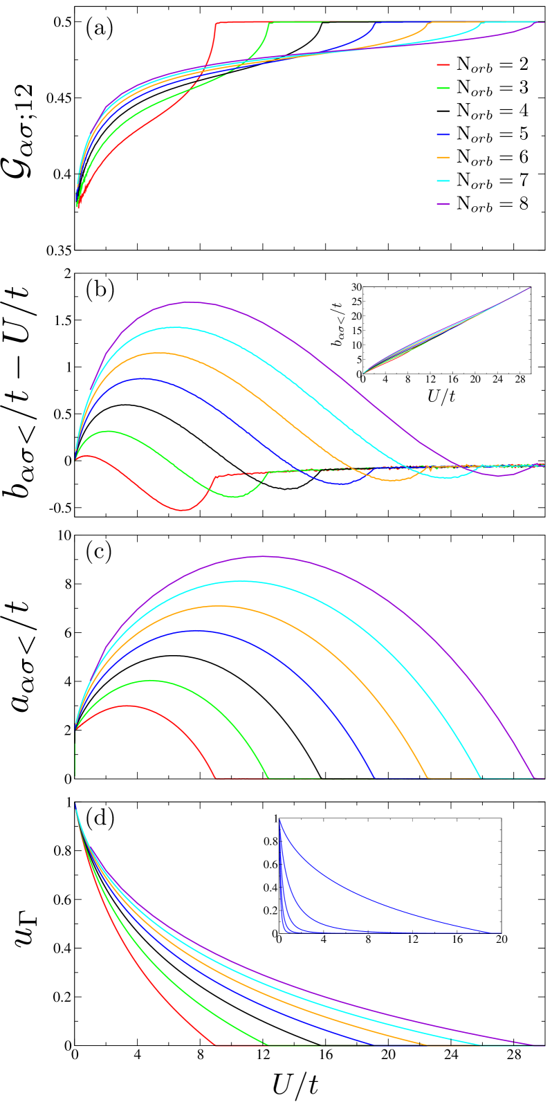
Figure 1: Optimized variational parameters of VDAT within the SCDA at $\mathcal{N}=3$ for the SU(2N${}_{\textrm{orb}}$) Hubbard model on the $d=\infty$ Bethe lattice at half filling and $T=0$, with N${}_{\textrm{orb}}=2-8$. The variational parameters $\mathcal{G}_{\alpha\sigma;12}$, $b_{\alpha\sigma<}$, and $u_{\Gamma}$ for $\Gamma$ with particle number N${}_{\textrm{orb}}-1$ are shown in panels $a$, $b$, and $d$, respectively, while the dependent parameters $a_{\alpha\sigma<}$ are shown in panel $c$. The inset of panel $d$ shows all $u_{\Gamma}$ for N${}_{\textrm{orb}}=5$, and the value monotonically decreases as the particle number of $\Gamma$ decreases from four to zero.

We now proceed to illustrate the gauge constrained implementation of VDAT within the SCDA at $\mathcal{N}=3$. We choose to study the SU(2N${}_{\textrm{orb}}$) Hubbard model, where $\hat{H}_{loc;i}=U\sum_{\ell<\ell^{\prime}}\hat{n}_{i\ell}\hat{n}_{i\ell^{\prime}}$ and $\ell=1,\dots,2\textmd{N}_{\textrm{orb}}$, in order to showcase the advantages of VDAT over DMFT for obtaining zero temperature results at large N${}_{\textrm{orb}}$. It should be noted that the SU(2N${}_{\textrm{orb}}$) symmetry can be exploited when evaluating the expectation values of local observables (i.e. Eq. 32), but for purposes of benchmarking the computational cost, we utilized the general algorithm which does not exploit the SU(2N${}_{\textrm{orb}}$) symmetry. Therefore, for a single evaluation of the SPD, the computational cost is the same as the general case. To provide a rough idea of the computational cost on a typical single processor core, when $\textrm{N}{}_{\textrm{orb}}\leq 3$ the cost of a single evaluation of the SPD is $10^{-4}$ seconds. For $\textrm{N}{}_{\textrm{orb}}>3$, the computational cost scales exponentially, requiring $10^{-3}$, 0.02, 0.1, and 3 seconds for $\textrm{N}{}_{\textrm{orb}}$ of 4, 5, 6, and 7, respectively. The timing difference between $\mathcal{N}=2$ and $\mathcal{N}=3$ is negligible in all the aforementioned cases. We study the SU(2N${}_{\textrm{orb}}$) Hubbard model on the $d=\infty$ Bethe lattice for N${}_{\textrm{orb}}$=2-8 at half filling and 2N${}_{\textrm{orb}}$=5 for all fillings. At half filling for N${}_{\textrm{orb}}$=2,4 we compare to a zero temperature extrapolation of published DMFT results using a quantum Monte-Carlo (QMC) impurity solver [2], while for 2N${}_{\textrm{orb}}$=5 we compare to published DMFT results using the numerical renormalization group (NRG) impurity solver [18]. All VDAT results in this paper are generated by a Julia implementation of the gauge constrained algorithm, which can treat general density-density interactions, and is available at [7].

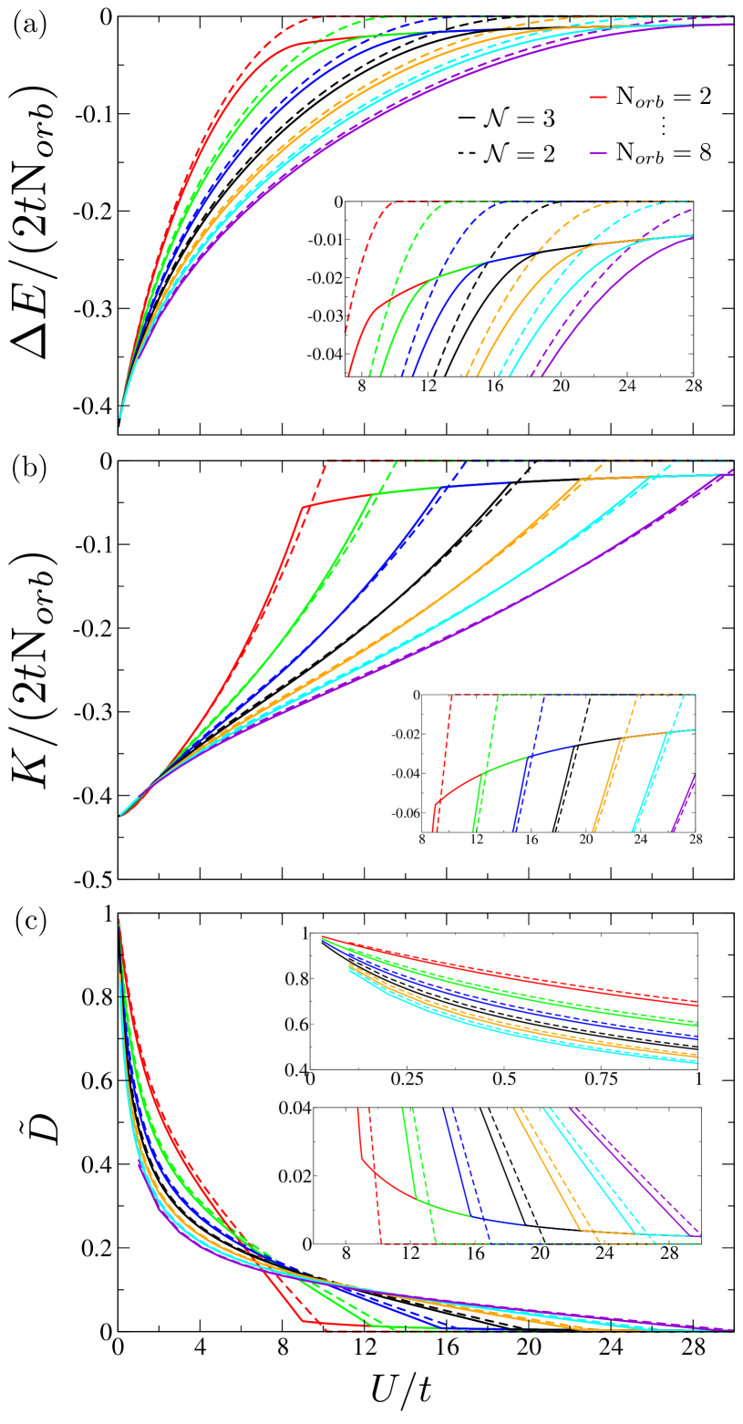
Figure 2: Static observables computed from VDAT within the SCDA at $\mathcal{N}=2$ (dashed lines) and $\mathcal{N}=3$ (solid lines) for the SU(2N${}_{\textrm{orb}}$) Hubbard model on the $d=\infty$ Bethe lattice at half filling and $T=0$, with N${}_{\textrm{orb}}=2-8$. The legend colors are identical to Figure 1. ($a$) Total energy difference per spin orbital vs. $U/t$, where $\Delta E=E(t,U)-E(0,U)$. ($b$) Kinetic energy per spin orbital vs. $U/t$. ($c$) Scaled double occupancy vs. $U/t$, where $\tilde{D}=(D-D_{at})/(D_{0}-D_{at})$; $D$, $D_{0}$, and $D_{at}$ are the double occupancies at the given $U/t$, the non-interacting value, and the atomic value, respectively.

We begin by considering the case of half filling for N${}_{\textrm{orb}}$=2-8, exceeding the number of orbitals that would be encountered for a $d$ or $f$ electron manifold relevant to strongly correlated electron materials. The basic aspects of the SU(2N${}_{\textrm{orb}}$) Hubbard model in $d=\infty$ are well understood: there is a metal-insulator transition (MIT) at a critical value of $U$, and this transition value increases with N${}_{\textrm{orb}}$. The signature of the MIT can be seen in the variational parameters of the SPD, and therefore it is instructive to examine $\mathcal{G}_{\alpha\sigma;12}$, $b_{\alpha\sigma<}$, and the local variational parameters $u=\{u_{\Gamma}\}$ (see Figure 1). It is also useful to explore the intermediate parameters $a_{\alpha\sigma<}$, which can be determined from the variational parameters. Because of the SU(2N${}_{\textrm{orb}}$) symmetry, the $\mathcal{G}_{\alpha\sigma;12}$, $b_{\alpha\sigma<}$, and $a_{\alpha\sigma<}$ are independent of $\alpha\sigma$, while $u_{\Gamma}$ only depends on the particle number of $\Gamma$. Furthermore, particle-hole symmetry at half filling dictates that $b_{\alpha\sigma<}=b_{\alpha\sigma>}$, $a_{\alpha\sigma<}=-a_{\alpha\sigma>}$, and $u_{\Gamma}=u_{\Gamma^{\prime}}$ if the sum of the particle numbers of $\Gamma$ and $\Gamma^{\prime}$ is 2N${}_{\textrm{orb}}$. Considering $\mathcal{G}_{\alpha\sigma;12}$, it begins at $U=0$ in the metallic phase with a value of roughly 0.37 and monotonically increases to 0.5 at the MIT, and is fixed at 0.5 in the insulating regime (see Figure 1a). Increasing the number of orbitals from N${}_{\textrm{orb}}$=2-8 has several effects. In the small $U$ regime, $\mathcal{G}_{\alpha\sigma;12}$ increases with N${}_{\textrm{orb}}$, enhancing the electronic correlations for larger N${}_{\textrm{orb}}$. Alternatively, increasing N${}_{\textrm{orb}}$ will increase the critical value of $U$ for the metal-insulator transition. The variational parameter $b_{\alpha\sigma<}$ turns out to be approximately equal to $U$, and therefore we also plot $b_{\alpha\sigma<}-U$ (see Figure 1b). The intermediate parameter $a_{\alpha\sigma<}$, which can be computed from the variational parameters, has a value of $2t$ for $U=0$, independent of N${}_{\textrm{orb}}$, and goes to zero in the insulating phase (see Figure 1c). The latter can be appreciated from Eq. 25, which dictates that the quasiparticle weight becomes zero when $a_{\alpha\sigma<}=a_{\alpha\sigma>}$ and $b_{\alpha\sigma<}=b_{\alpha\sigma>}$. For a given N${}_{\textrm{orb}}$, there is an arbitrary coefficient for the interacting projector which can be fixed by choosing $u_{\Gamma}=1$ when the particle number of $\Gamma$ is N${}_{\textrm{orb}}$. Therefore, there are N${}_{\textrm{orb}}$ independent local variational parameters $u_{\Gamma}$ for $\Gamma$ with particle number equal to $0,\dots,\textrm{N}_{\textrm{orb}}-1$. For a given N${}_{\textrm{orb}}$, we plot the $u_{\Gamma}$ where the particle number for $\Gamma$ is N${}_{\textrm{orb}}$-1 (see Figure 1d), in addition to all $u_{\Gamma}$ for $\textrm{N}_{\textrm{orb}}=5$. The $u_{\Gamma}$ for $\Gamma$ with particle number N${}_{\textrm{orb}}$-1 goes to zero in the insulating phase.

We now consider the total energy, where we explore both $\mathcal{N}=2$ and $\mathcal{N}=3$ (see Fig. 2a). For clarity, we plot $\Delta E=E(t,U)-E(0,U)$ divided by the number of spin orbitals. The $\mathcal{N}=3$ results are always lower in energy than the $\mathcal{N}=2$ results, as is required by the variational principle. Furthermore, the $\mathcal{N}=3$ results resolve the well known deficiency of the $\mathcal{N}=2$ results in the insulating regime. Interestingly, in the small and large $U$ regimes, the quantity $\Delta E/(2\textrm{N}_{\textrm{orb}})$ is largely independent of $\textrm{N}_{\textrm{orb}}$, while in the intermediate regime it decreases with $\textrm{N}_{\textrm{orb}}$. Similar behavior is observed in the kinetic energy per orbital (see Fig. 2b). The double occupancy $D$ determines the interaction energy, and for convenience we plot the scaled double occupancy $\tilde{D}=(D-D_{at})/(D_{0}-D_{at})$, where $D_{0}$ and $D_{at}$ are the non-interacting and atomic double occupancy, respectively (see Fig. 2c). In the small $U$ regime, the scaled double occupancy decreases with $\textrm{N}_{\textrm{orb}}$, while in the large $U$ regime it is independent of $\textrm{N}_{\textrm{orb}}$.

It is also interesting to evaluate the quasiparticle weight as a function of $U/t$, which determines the critical value of $U$ for the MIT (see Fig. 3a). The $\mathcal{N}=2$ result always produces a large quasiparticle weight than $\mathcal{N}=3$, and therefore produces a larger critical value of $U$ for the MIT. Interestingly, for $\mathcal{N}=3$ at approximately $U/t=1$, the quasiparticle weight is insensitive to $\textrm{N}_{\textrm{orb}}$, and a similar effect is observed for $\mathcal{N}=2$ at a slightly large value of $U/t$. We also examine the transition value $U_{c}/t$ as a function of $\textrm{N}_{\textrm{orb}}$ and compare to the previously published scaling relation [2] $U_{c}/t=1.7(2\textrm{N}_{\textrm{orb}}+1)(1+0.166\textrm{N}_{\textrm{orb}}^{-1})$ extracted from DMFT calculations which use QMC as the impurity solver (see Figure 3$b$). The $\mathcal{N}=2$ case recovers the previously published results of the Gutzwiller approximation [19, 9], yielding a linear relation. Interestingly, $\mathcal{N}=3$ also produces a nearly linear result, but the result is shifted downward, nearly coinciding with the DMFT extrapolation.

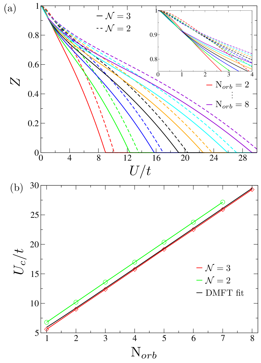
Figure 3: Results for VDAT within the SCDA at $\mathcal{N}=2$ and $\mathcal{N}=3$ for the SU(2N${}_{\textrm{orb}}$) Hubbard model on the $d=\infty$ Bethe lattice at half filling and $T=0$, with N${}_{\textrm{orb}}=2-8$. ($a$) Quasiparticle weight. The legend is identical to Figure 1. ($b$) The critical value of $U$ for the MIT, denoted $U_{c}$, as a function of $\textrm{N}_{\textrm{orb}}$. The DMFT curve is a plot of a previously published fit to DMFT results [2], given as $U_{c}/t=1.7(2\textrm{N}_{\textrm{orb}}+1)(1+0.166\textrm{N}_{\textrm{orb}}^{-1})$.

We now proceed to compare the total energy at half filling and zero temperature from VDAT and DMFT. Given that the previously published DMFT results are at a finite temperature [2], a quadratic fit assuming $E(T)-E(0)\propto T^{2}$ was used to extrapolate to zero temperature (see Fig. 4). We were only able to examine select cases where the QMC data sufficiently resembled a quadratic. For $\textrm{N}_{\textrm{orb}}=2$, we present VDAT results for $\mathcal{N}=2-4$, which were previously published in Ref. [4], while for $\textrm{N}_{\textrm{orb}}=4$ we present VDAT results for $\mathcal{N}=2-3$. As required by the variational principle, the energy within VDAT monotonically decreases with increasing $\mathcal{N}$. The dramatic improvement of $\mathcal{N}=3$ over $\mathcal{N}=2$ is clearly illustrated, and it should be recalled that these two cases have a similar computational cost.

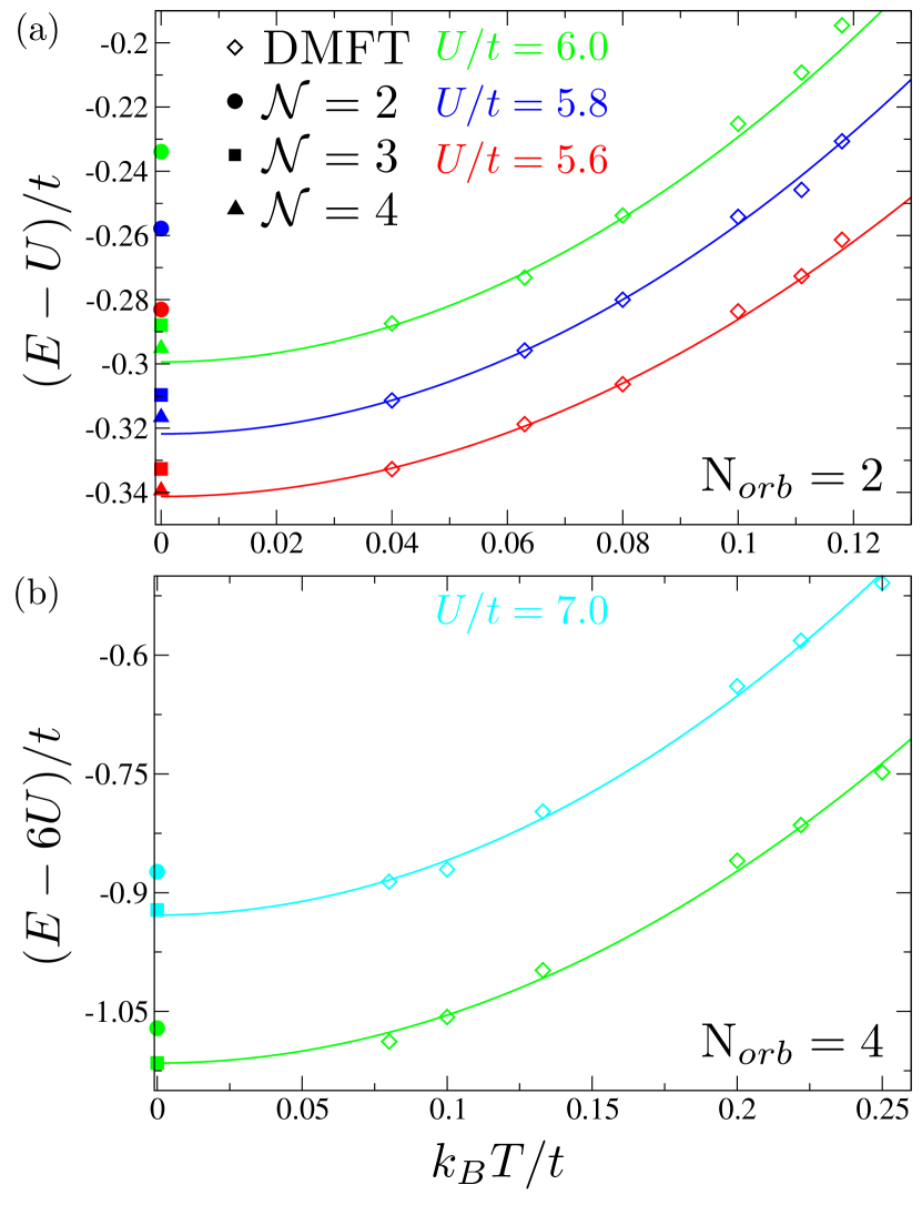
Figure 4: The total energy of the SU(2N${}_{\textrm{orb}}$) Hubbard model on the $d=\infty$ Bethe lattice at half filling from published DMFT calculations solved using QMC at a finite temperature [2] and VDAT within the SCDA at zero temperature using $\mathcal{N}=2-4$, with N${}_{\textrm{orb}}=2$ in panel $a$ and N${}_{\textrm{orb}}=4$ in panel $b$. The lines are a fit to the DMFT results assuming $E(T)-E(0)\propto T^{2}$.

Finally, we evaluate the doping dependence of the total energy, in addition to the corresponding first and second derivatives, using VDAT with $\mathcal{N}=2$ and $\mathcal{N}=3$. We compare to a previously published DMFT study which used the NRG impurity solver [18] to study $2\textrm{N}_{\textrm{orb}}=5$ for $U/t=6$ and $U/t=14$ (see Fig. 5), where $U/t=6$ is a metal at all densities and $U/t=14$ undergoes an MIT at the integer fillings of $n=0.2$ and $n=0.4$. We first compare the total energy, where the variational principle guarantees that the energy monotonically decreases from $\mathcal{N}=2$ to $\mathcal{N}=3$ to the numerically exact solution given by DMFT solved within NRG (see Fig. 5, panel $a$). It should be noted the DMFT study did not provide the total energy, and we obtained it by numerically integrating the chemical potential over the density. For clarity, we plot $\Delta E/t$ where $\Delta E=E(t,U)-E(0,U)$ and $E(t,U)$ is the total energy evaluated at a given density. Overall, $\mathcal{N}=3$ yields a dramatic improvement over $\mathcal{N}=2$, especially at integer fillings. Interestingly, the trends in the absolute error of the total energy are notably different for $\mathcal{N}=2$ and $\mathcal{N}=3$, where the former has the largest absolute error at integer filling while the latter has the largest absolute error midway between integer fillings. The trend for $\mathcal{N}=3$ might be attributed to the efficacy of the kinetic projector for capturing superexchange at integer filling. We proceed to compare the chemical potential, which is the derivative of the energy with respect to the density, as a function of density (see Fig. 5, panel $b$). Within VDAT, the chemical potential was obtained using finite difference to take the first derivative of the total energy with respect to the density, and a grid spacing of 0.002 was used for $0.02<n_{\alpha\sigma}\leq 0.5$ while 0.0001 was used for $n_{\alpha\sigma}<0.02$. For clarity, we plot $\Delta\mu/U$ where $\Delta\mu=\mu-2U$. The Mott transition can clearly be identified as a discontinuity in the chemical potential at integer fillings. While $\mathcal{N}=2$ is reasonable overall, there are clear discrepancies near the MIT (see insets for absolute error in $\Delta\mu/U$), and $\mathcal{N}=3$ largely resolves these issues. However, it should be recalled that unlike the total energy, the convergence of the chemical potential is not necessarily monotonic in $\mathcal{N}$. For example, in the case of $U/t=14$ and $n\rightarrow 0.2^{-}$, the total energy for $\mathcal{N}=2$ is substantially larger than $\mathcal{N}=3$, yet the chemical potential for $\mathcal{N}=2$ is much closer to the exact solution. To further scrutinize these same results from another viewpoint, we examine $U\partial n/\partial\mu$ as a function of density (see Fig. 5$c$). Within VDAT, $\partial\mu/\partial n$ was obtained using finite difference to take the second derivative of the total energy, and the same grid spacing was used as in the case of the chemical potential. For the low density region $n_{\alpha\sigma}<0.1$, the $\mathcal{N}=3$ results were smoothed using a spline interpolation. Similar to the chemical potential, the convergence of this quantity is not necessarily monotonic in $\mathcal{N}$, and the same conclusions can be drawn.

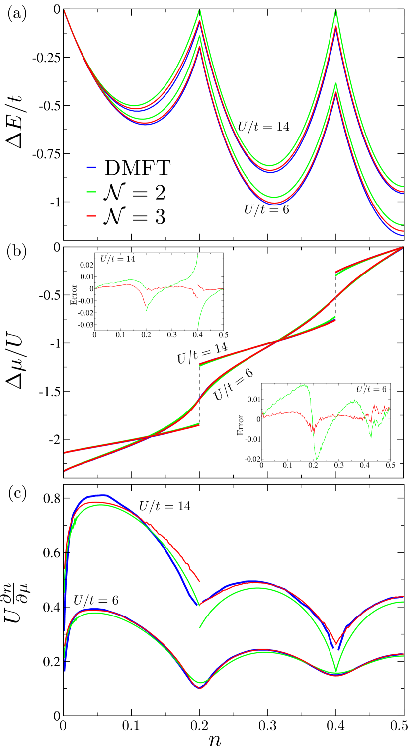
Figure 5: Doping dependent results of the SU(2N${}_{\textrm{orb}}$) Hubbard model on the $d=\infty$ Bethe lattice at zero temperature from published DMFT calculations solved using NRG [18] and VDAT within the SCDA using $\mathcal{N}=2$ and $\mathcal{N}=3$, with 2N${}_{\textrm{orb}}=5$. (panel $a$) Total energy difference $\Delta E$ vs. density, where $\Delta E=E(t,U)-E(0,U)$. The DMFT curve is obtained by integrating the chemical potential over density. (panel $b$) $\Delta\mu/U$ vs. density, where $\Delta\mu=\mu-2U$. The insets plot the absolute error in $\Delta\mu/U$ vs. density. (panel $c$) The derivative $\partial n/\partial\mu$ times $U$ vs. the density.

IV Conclusions

In this paper, we proposed a gauge constrained algorithm to evaluate the SPD ansatz at $\mathcal{N}=3$ within the SCDA for the multi-orbital Hubbard model. The key feature of this algorithm is that it automatically satisfies the self-consistency condition of the SCDA using the gauge freedom of the SPD, greatly facilitating the minimization over the variational parameters. Interestingly, the gauge constrained algorithm yields a simple analytical form of the single particle density matrix of the optimized SPD ansatz. The convenient mathematical form of the gauge constrained algorithm greatly simplifies the implementation of VDAT within the SCDA when treating a large number of orbitals. In order to showcase the power of the gauge constrained algorithm, we studied the SU(2N${}_{\textrm{orb}}$) Hubbard model at zero temperature on the Bethe lattice in $d=\infty$ for $\textrm{N}_{\textrm{orb}}=2-8$, and compare to numerically exact DMFT results where available. While the symmetry of the SU(2N${}_{\textrm{orb}}$) Hubbard model greatly reduces the computational cost for solving the DMFT impurity model, computational limitations still restrict most studies to relatively small values of N${}_{\textrm{orb}}$. A DMFT study using a numerical renormalization group impurity solver presented results up to $2\textrm{N}_{\textrm{orb}}=5$ [18], while a study using a quantum Monte-Carlo impurity solver presented finite temperature results up to $\textrm{N}_{\textrm{orb}}=8$ [2]; though the latter results were at relatively high temperatures and appear to have nontrivial stochastic error. Therefore, our successful execution of $\textrm{N}_{\textrm{orb}}=8$ showcases the utility of the gauge constrained algorithm for executing VDAT within the SCDA at $\mathcal{N}=3$. At half filling, we evaluated the kinetic energy, interaction energy, and quasiparticle weight as a function of $U/t$. For the doped case, we evaluated the density as a function of the chemical potential, in addition to the derivative, at various values of $U/t$. As expected, $\mathcal{N}=3$ yields a dramatic improvement over $\mathcal{N}=2$, at a similar computational cost. The successful computation of the ground state energy for the $\textrm{N}_{\textrm{orb}}=7$ Hubbard model on a single processor core in under one hour demonstrates the viability of VDAT to study realistic $f$-electron systems. The technical developments in this work are a key step forward towards studying realistic Hamiltonians of complex strongly correlated electron materials.

V Acknowledgements

We thank Shuxiang Yang for useful discussions about the manuscript. This work was supported by the Columbia Center for Computational Electrochemistry. This research used resources of the National Energy Research Scientific Computing Center, a DOE Office of Science User Facility supported by the Office of Science of the U.S. Department of Energy under Contract No. DE-AC02-05CH11231.

Appendix A Solving multi-orbital Hubbard model with a density constraint

It is often desirable to solve a Hamiltonian with fixed densities for the spin orbitals, which can be efficiently executed by reparametrizing the variational parameters $u$. We begin by realizing that the vector space associated with $u$ can be constructed as a direct product of two dimensional vector spaces associated with each spin orbital. For an operator in the compound space $\textrm{\@text@baccent{$\hat{O}$}}=\prod_{\alpha\sigma}\textrm{\@text@baccent{$\hat{O}$}}_{\alpha\sigma}$, the representation in the $u$ basis can be constructed as

$$(\textrm{\@text@baccent{$\hat{O}$}})_{u}=(\textrm{\@text@baccent{$\hat{O}$}}_{1\uparrow})_{u;1\uparrow}\otimes\dots\otimes(\textrm{\@text@baccent{$\hat{O}$}}_{N_{\textrm{orb}}\downarrow})_{u;N_{\textrm{orb}}\downarrow}.$$ (98)

Using this relation, equations 35 and 37 are recast as

$$\left(\textrm{\@text@baccent{$\hat{1}$}}\right)_{u}= \left(\textrm{\@text@baccent{$\hat{1}$}}\right)_{u;1\uparrow}\otimes\cdots\otimes\left(\textrm{\@text@baccent{$\hat{1}$}}\right)_{u;N_{\textrm{orb}}\downarrow},$$ (99)

$$(\textrm{\@text@baccent{$\hat{a}$}}_{\alpha\sigma}^{\dagger\left(\tau\right)}\textrm{\@text@baccent{$\hat{a}$}}_{\alpha\sigma}^{\left(\tau^{\prime}\right)})_{u}= \left(\textrm{\@text@baccent{$\hat{1}$}}\right)_{u;1\uparrow}\otimes\cdots$$

$$\otimes(\textrm{\@text@baccent{$\hat{a}$}}_{\alpha\sigma}^{\dagger\left(\tau\right)}\textrm{\@text@baccent{$\hat{a}$}}_{\alpha\sigma}^{\left(\tau^{\prime}\right)})_{u;\alpha\sigma}\dots\otimes\left(\textrm{\@text@baccent{$\hat{1}$}}\right)_{u;N_{\textrm{orb}}\downarrow},$$ (100)

where

$$[\left(\textrm{\@text@baccent{$\hat{1}$}}\right)_{u;\alpha\sigma}]_{\Gamma_{\alpha\sigma}\Gamma^{\prime}_{\alpha\sigma}}=p_{\alpha\sigma}\left(\Gamma_{\alpha\sigma},\Gamma_{\alpha\sigma}^{\prime}\right),$$ (101)

$$[(\textrm{\@text@baccent{$\hat{a}$}}_{\alpha\sigma}^{\dagger(\tau)}\textrm{\@text@baccent{$\hat{a}$}}_{\alpha\sigma}^{(\tau^{\prime})})_{u;\alpha\sigma}]_{\Gamma_{\alpha\sigma}\Gamma^{\prime}_{\alpha\sigma}}=g_{\alpha\sigma}^{\tau\tau^{\prime}}\left(\Gamma_{\alpha\sigma},\Gamma^{\prime}_{\alpha\sigma}\right),$$ (102)

where $p_{\alpha\sigma}\left(\Gamma_{\alpha\sigma},\Gamma_{\alpha\sigma}^{\prime}\right)$ and $g_{\alpha\sigma}^{\tau\tau^{\prime}}\left(\Gamma_{\alpha\sigma},\Gamma^{\prime}_{\alpha\sigma}\right)$ are defined in equations 36 and 38, respectively. The relevant matrices which will be needed to constrain the orbital density are

$$\left(\textrm{\@text@baccent{$\hat{1}$}}\right)_{u;\alpha\sigma}=\left(\begin{array}[]{cc}\mathcal{G}_{\alpha\sigma,1,2}^{2}+\frac{1}{4}&\frac{1}{4}-\mathcal{G}_{\alpha\sigma,1,2}^{2}\\ \frac{1}{4}-\mathcal{G}_{\alpha\sigma,1,2}^{2}&\mathcal{G}_{\alpha\sigma,1,2}^{2}+\frac{1}{4}\end{array}\right),$$ (105)

$$\left(\textrm{\@text@baccent{$\hat{a}$}}_{\alpha\sigma}^{\dagger\left(1\right)}\textrm{\@text@baccent{$\hat{a}$}}_{\alpha\sigma}^{\left(1\right)}\right)_{u;\alpha\sigma}=\left(\begin{array}[]{cc}0&0\\ \frac{1}{4}-\mathcal{G}_{\alpha\sigma,1,2}^{2}&\mathcal{G}_{\alpha\sigma,1,2}^{2}+\frac{1}{4}\end{array}\right),$$ (108)

$$\left(\textrm{\@text@baccent{$\hat{a}$}}_{\alpha\sigma}^{\dagger\left(2\right)}\textrm{\@text@baccent{$\hat{a}$}}_{\alpha\sigma}^{\left(2\right)}\right)_{u;\alpha\sigma}=\left(\begin{array}[]{cc}0&\frac{1}{4}-\mathcal{G}_{\alpha\sigma,1,2}^{2}\\ 0&\mathcal{G}_{\alpha\sigma,1,2}^{2}+\frac{1}{4}\end{array}\right).$$ (111)

In summary, Eq. 98 provides a simple mathematical structure to construct $(\textrm{\@text@baccent{$\hat{O}$}})_{u}$.

We now proceed to reparametrize the variational parameters $u$. In general, one can introduce a linear transformation over the variational parameters as $u=Vw$, and by requiring $w^{T}(\textrm{\@text@baccent{$\hat{O}$}})_{w}w=u^{T}(\textrm{\@text@baccent{$\hat{O}$}})_{u}u,$ a new matrix form is obtained as

$$(\textrm{\@text@baccent{$\hat{O}$}})_{w}\equiv V^{T}(\textrm{\@text@baccent{$\hat{O}$}})_{u}V.$$ (112)

In order to preserve the direct product structure of $(\textrm{\@text@baccent{$\hat{O}$}})_{w}$, the transformation is constructed as $V=V_{1\uparrow}\otimes\cdots\otimes V_{\textrm{N}_{\textrm{orb}}\downarrow}$, resulting in

$$(\textrm{\@text@baccent{$\hat{O}$}})_{w}=(\textrm{\@text@baccent{$\hat{O}$}}_{1\uparrow})_{w;1\uparrow}\otimes\dots\otimes(\textrm{\@text@baccent{$\hat{O}$}}_{\textrm{N}_{\textrm{orb}}\downarrow})_{w;\textrm{N}_{\textrm{orb}}\downarrow},$$ (113)

$$(\textrm{\@text@baccent{$\hat{O}$}}_{\alpha\sigma})_{w;\alpha\sigma}\equiv V_{\alpha\sigma}^{T}(\textrm{\@text@baccent{$\hat{O}$}}_{\alpha\sigma})_{u;\alpha\sigma}V_{\alpha\sigma}.$$ (114)

In order to ensure that $(\textrm{\@text@baccent{$\hat{1}$}})_{w;\alpha\sigma}$ is the identity matrix and the symmetric part of $(\textrm{\@text@baccent{$\hat{a}$}}_{\alpha\sigma}^{\dagger\left(1\right)}\textrm{\@text@baccent{$\hat{a}$}}_{\alpha\sigma}^{\left(1\right)})_{w;\alpha\sigma}$ is diagonal, we have

$$\boldsymbol{V}_{\alpha\sigma}=\frac{1}{\sqrt{2}}\left(\begin{array}[]{cc}\frac{1}{2\mathcal{G}_{\alpha\sigma,1,2}}+1&1-\frac{1}{2\mathcal{G}_{\alpha\sigma,1,2}}\\ 1-\frac{1}{2\mathcal{G}_{\alpha\sigma,1,2}}&\frac{1}{2\mathcal{G}_{\alpha\sigma,1,2}}+1\end{array}\right),$$ (115)

thus completely defining the reparametrization. One of the necessary reparameterized matrix elements is

$$\boldsymbol{n}_{w;\alpha\sigma} \equiv\frac{1}{2}\left((\textrm{\@text@baccent{$\hat{a}$}}_{\alpha\sigma}^{\dagger\left(1\right)}\textrm{\@text@baccent{$\hat{a}$}}_{\alpha\sigma}^{\left(1\right)})_{w;\alpha\sigma}+(\textrm{\@text@baccent{$\hat{a}$}}_{\alpha\sigma}^{\dagger\left(1\right)}\textrm{\@text@baccent{$\hat{a}$}}_{\alpha\sigma}^{\left(1\right)})_{w;\alpha\sigma}^{T}\right)$$

$$=\left(\begin{array}[]{cc}-\frac{\left(1-2\mathcal{G}_{\alpha\sigma,1,2}\right){}^{2}}{8\mathcal{G}_{\alpha\sigma,1,2}}&0\\ 0&\frac{\left(2\mathcal{G}_{\alpha\sigma,1,2}+1\right){}^{2}}{8\mathcal{G}_{\alpha\sigma,1,2}}\end{array}\right),$$ (118)

and the others are provided in Supplementary Material [1].

We now proceed to constrain the density for each spin orbital, and we begin by considering the case where the interacting projector is a non-interacting density matrix, which can be written as

$$w_{\Gamma;0}^{2}=\prod_{\alpha\alpha}\left(\left(1-n_{\alpha\sigma;eff}\right)\left(1-\Gamma_{\alpha\sigma}\right)+n_{\sigma\alpha;eff}\Gamma_{\alpha\sigma}\right),$$ (119)

where $n_{\alpha\sigma;eff}$ can be determined from

$$\textrm{Tr}\left(\boldsymbol{n}_{w;\alpha\sigma}\left(\begin{array}[]{cc}1-n_{\alpha\sigma;eff}&0\\ 0&n_{\sigma\alpha;eff}\end{array}\right)\right) =n_{\alpha\sigma},$$ (122)

which can be solved as

$$n_{\alpha\sigma,\text{eff}}=\frac{2\left(2n_{\alpha\sigma}-1\right)\mathcal{G}_{\alpha\sigma,1,2}}{4\mathcal{G}_{\alpha\sigma,1,2}^{2}+1}+\frac{1}{2}.$$ (123)

Subsequently, $2^{2\textrm{N}_{\textrm{orb}}}-\left(1+2\textrm{N}_{\textrm{orb}}\right)$ variational parameters $x_{\eta}$ can be introduced to describe the deviations from $w_{\Gamma;0}^{2}$, which do not change the density or the normalization. It is then useful to define a $2^{2\textrm{N}_{\textrm{orb}}}\times 2^{2\textrm{N}_{\textrm{orb}}}$ matrix $V_{\Gamma\eta}$ as

$$V_{\Gamma i(\{\alpha_{1}\sigma_{1},\dots,\alpha_{n}\sigma_{n}\})}=\prod_{j=1}^{n}(\Gamma_{\alpha_{j}\sigma_{j}}-\frac{1}{2}),$$ (124)

where $i(\{\alpha_{1}\sigma_{1},\dots,\alpha_{n}\sigma_{n}\})=1,\dots,2^{2\textrm{N}_{\textrm{orb}}}$ is a convention for indexing all subsets of $\{1\uparrow,1\downarrow,\dots,\textrm{N}_{\textrm{orb}}\uparrow,\textrm{N}_{\textrm{orb}}\downarrow\}$, and $n=0,\dots,2\textrm{N}_{\textrm{orb}}$ denotes the number of spin orbitals contained in a given subset. A convenient convention for sorting the subsets is first sorting by increasing cardinality and then by the binary interpretation of the subset. The subsets with cardinality greater than one form $2^{2\textrm{N}_{\textrm{orb}}}-\left(1+2\textrm{N}_{\textrm{orb}}\right)$ orthogonal vectors that do not change the normalization or the orbital occupation. A similar approach has been used to represent the Bernoulli distribution [28]. A general interacting projector that is constrained to the given orbital occupation can be parameterized as

$$w_{\Gamma}^{2}=w_{\Gamma;0}^{2}+\sum_{\eta=2+2\textrm{N}_{\textrm{orb}}}^{2^{2\textrm{N}_{\textrm{orb}}}}V_{\Gamma\eta}x_{\eta},$$ (125)

where $x_{\eta}$ are real numbers that are constrained by the condition that $\omega_{\Gamma}^{2}\geq 0$. For example, $\textrm{N}_{\textrm{orb}}=1$ results in one independent variational parameter $x$, yielding

$$w_{1}^{2}=\left(1-n_{\uparrow;eff}\right)\left(1-n_{\downarrow eff}\right)+\frac{1}{4}x,$$ (126)

$$w_{2}^{2}=\left(1-n_{\uparrow;eff}\right)n_{\downarrow eff}-\frac{1}{4}x,$$ (127)

$$w_{3}^{2}=n_{\uparrow;eff}\left(1-n_{\downarrow eff}\right)-\frac{1}{4}x,$$ (128)

$$w_{4}^{2}=n_{\uparrow;eff}n_{\downarrow eff}+\frac{1}{4}x,$$ (129)

where $x\in[x_{\textrm{min}},x_{\textrm{max}}]$ and

$$x_{\textrm{min}}=-4\min((1-n_{\uparrow;eff})(1-n_{\downarrow eff}),n_{\uparrow;eff}n_{\downarrow eff}),$$ (130)

$$x_{\textrm{max}}=4\min((1-n_{\uparrow;eff})n_{\downarrow eff},n_{\uparrow;eff}(1-n_{\downarrow eff})).$$ (131)

Finally, the ground state energy can be obtained as

$$E=\min_{\mathcal{G}_{12},x,\bm{b}}\Big{(} \int dk\epsilon_{k\alpha\sigma}n_{k\alpha\sigma}\left(\bm{a},\bm{b}\right)+E_{loc}\left(\mathcal{G}_{12},x,\bm{b}\right)\Big{)},$$ (132)

where $x=\{x_{\eta}\}$ and $\bm{a}$ is determined from $\left\{n_{\alpha\sigma}\right\}$, $\mathcal{G}_{12}$, $x$, and $\bm{b}$.

Appendix B the gauge constrained algorithm using general local projectors

In this paper, we have assumed that the interacting projector can be written as a linear combination of diagonal Hubbard operators in the basis $\alpha\sigma$, and that $\boldsymbol{\mathcal{G}}$ is diagonal in basis $\alpha\sigma$. Here we outline how to treat the general case, starting with the first assumption. A general local interacting projector can be an arbitrary linear combination of all possible Hubbard operators, including off-diagonal Hubbard operators. A general Hubbard operator can be constructed as

$$\hat{P}_{i\Gamma}=\prod_{\alpha\sigma} \Big{(}\delta_{\Gamma_{\alpha\sigma},0}(1-\hat{n}_{i\alpha\sigma})+\delta_{\Gamma_{\alpha\sigma},1}\hat{n}_{i\alpha\sigma}$$

$$+\delta_{\Gamma_{\alpha\sigma},2}\hat{a}_{i\alpha\sigma}^{\dagger}+\delta_{\Gamma_{\alpha\sigma},3}\hat{a}_{i\alpha\sigma}\Big{)},$$ (133)

$$=\prod_{\alpha\sigma} \hat{P}_{i\alpha\sigma;\Gamma_{\alpha\sigma}},$$ (134)

where $\Gamma-1=\left(\Gamma_{1\uparrow}\dots\Gamma_{\textrm{N}_{\textrm{orb}}\downarrow}\right)_{4}$ and $\Gamma=1,\dots,4^{2\textrm{N}_{\textrm{orb}}}$. The most general interacting projector can be constructed as $\hat{P}_{i}(u)=\sum_{\Gamma}u_{\Gamma}\hat{P}_{i\Gamma}$. However, given that we require $\hat{P}_{i}(u)$ to obey certain symmetries and conservation relations, some $u_{\Gamma}$ may be zero. In order to evaluate $\langle\textrm{\@text@baccent{$\hat{P}$}}_{i}^{\left(1\right)}\textrm{\@text@baccent{$\hat{P}$}}_{i}^{\left(2\right)}\textrm{\@text@baccent{$\hat{O}$}}\rangle_{\textrm{\@text@baccent{$\hat{\rho}$}}_{loc;i,0}}$, we first consider

$$\textrm{\@text@baccent{$\hat{O}$}}=\prod_{\alpha\sigma}\textrm{\@text@baccent{$\hat{O}$}}_{\alpha\sigma},$$ (135)

where $\textrm{\@text@baccent{$\hat{O}$}}_{\alpha\sigma}$ is a single product in terms of $\textrm{\@text@baccent{$\hat{a}$}}_{i\alpha\sigma}^{\dagger\left(\tau\right)}$ and $\textrm{\@text@baccent{$\hat{a}$}}_{i\alpha\sigma}^{\left(\tau\right)}$, yielding

$$\left\langle\textrm{\@text@baccent{$\hat{P}$}}_{i}^{\left(1\right)}\textrm{\@text@baccent{$\hat{P}$}}_{i}^{\left(2\right)}\textrm{\@text@baccent{$\hat{O}$}}\right\rangle_{\textrm{\@text@baccent{$\hat{\rho}$}}_{loc;i,0}} =\sum_{\Gamma\Gamma^{\prime}}u_{\Gamma}u_{\Gamma^{\prime}}\left\langle\textrm{\@text@baccent{$\hat{P}$}}_{i\Gamma}^{\left(1\right)}\textrm{\@text@baccent{$\hat{P}$}}_{i\Gamma^{\prime}}^{\left(2\right)}\textrm{\@text@baccent{$\hat{O}$}}\right\rangle_{\textrm{\@text@baccent{$\hat{\rho}$}}_{loc;i,0}},$$ (136)

where

$$\left\langle\textrm{\@text@baccent{$\hat{P}$}}_{i\Gamma}^{\left(1\right)}\textrm{\@text@baccent{$\hat{P}$}}_{i\Gamma^{\prime}}^{\left(2\right)}\textrm{\@text@baccent{$\hat{O}$}}\right\rangle_{\textrm{\@text@baccent{$\hat{\rho}$}}_{loc;i,0}}$$

$$=\left\langle\prod_{\alpha\sigma}\textrm{\@text@baccent{$\hat{P}$}}_{i\alpha\sigma;\Gamma_{\alpha\sigma}}^{\left(1\right)}\prod_{\alpha\sigma}\textrm{\@text@baccent{$\hat{P}$}}_{i\alpha\sigma;\Gamma^{\prime}_{\alpha\sigma}}^{\left(2\right)}\prod_{\alpha\sigma}\textrm{\@text@baccent{$\hat{O}$}}_{\alpha\sigma}\right\rangle_{\textrm{\@text@baccent{$\hat{\rho}$}}_{loc;i,0}}$$ (137)

$$=\theta\left(\textrm{\@text@baccent{$\hat{O}$}},\Gamma,\Gamma^{\prime}\right)\prod_{\alpha\sigma}\left\langle\textrm{\@text@baccent{$\hat{P}$}}_{i\alpha\sigma;\Gamma_{\alpha\sigma}}^{\left(1\right)}\textrm{\@text@baccent{$\hat{P}$}}_{i\alpha\sigma;\Gamma^{\prime}_{\alpha\sigma}}^{\left(2\right)}\textrm{\@text@baccent{$\hat{O}$}}_{\alpha\sigma}\right\rangle_{\textrm{\@text@baccent{$\hat{\rho}$}}_{loc;i,0}},$$ (138)

where $\theta(\textrm{\@text@baccent{$\hat{O}$}},\Gamma,\Gamma^{\prime})=\pm 1$ and is determined by tracking the sign when ordering the expression from Eq. 137 to Eq. 138. For a general operator $̱\hat{O}$, one can always decompose it into a sum of operators which has the form of Eq 135 and apply the above formulas.

In order to treat a general $\boldsymbol{\mathcal{G}}$ and a general operator $̱\hat{O}$, one must straightforwardly apply Wick’s theorem to evaluate expectation values [5], though the resulting gauge constrained algorithm will be more complicated. For example, simple closed form equations such as Eq. 25 may not be obtained, requiring a numerical minimization to obtain the density distribution.

Appendix C Understanding how the $\mathcal{N}=3$ gauge constrained algorithm with a restricted kinetic projector reduces to $\mathcal{N}=2$

In Ref. [5], we illustrated how the SCDA at $\mathcal{N}=2$ using the Gutzwiller gauge recovers the Gutzwiller approximation. In the present work where we address $\mathcal{N}=3$, the gauge constrained algorithm uses a different type of gauge. Therefore, it is interesting to see how the $\mathcal{N}=3$ gauge constrained algorithm with a restricted kinetic projector can recover the Gutzwiller approximation. In particular, the restricted kinetic projector will force the density distribution to be flat both above and below the fermi surface. We begin by assuming

$$\bm{\mathcal{G}}_{\alpha\sigma}=\left(\begin{array}[]{ccc}\frac{1}{2}&\frac{1}{2}&\frac{1}{2}\\ -\frac{1}{2}&\frac{1}{2}&\frac{1}{2}\\ -\frac{1}{2}&-\frac{1}{2}&\frac{1}{2}\end{array}\right),$$ (139)

which is motivated by the Gutzwiller gauge. The canonical discrete action of $\bm{\mathcal{G}}_{\alpha\sigma}$ corresponds to an SPD [5], which is the product of three identity operators, and we can write the $A$ block for interacting Green’s function as

$$\boldsymbol{g}_{loc,\alpha\sigma;A}=\left(\begin{array}[]{cc}n_{\alpha\sigma}&a_{\alpha\sigma}r_{\alpha\sigma}\\ -a_{\alpha\sigma}r_{\alpha\sigma}&n_{\alpha\sigma}\end{array}\right),$$ (140)

where $a_{\alpha\sigma}=\sqrt{\left(1-n_{\alpha\sigma}\right)n_{\alpha\sigma}}$ and $r_{\alpha\sigma}$ denotes the renormalization for the off-diagonal elements of the A-block compared to the reference interacting Green’s function

$$\boldsymbol{g}_{loc,\alpha\sigma;A;ref}=\left(\begin{array}[]{cc}n_{\alpha\sigma}&a_{\alpha\sigma}\\ -a_{\alpha\sigma}&n_{\alpha\sigma}\end{array}\right),$$ (141)

which corresponds to the case where $\hat{P}$ is non-interacting, denoted as $\hat{P}_{0}$ . The $\hat{P}_{0}$ is chosen such that

$$\frac{\text{Tr}\left(\hat{P}_{0}^{2}\hat{n}_{\alpha\sigma}\right)}{\text{Tr}\left(\hat{P}_{0}^{2}\right)}=\frac{\text{Tr}\left(\hat{P}^{2}\hat{n}_{\alpha\sigma}\right)}{\text{Tr}\left(\hat{P}^{2}\right)}=n_{\alpha\sigma},$$ (142)

and $r_{\alpha\sigma}$ is given as

$$r_{\alpha\sigma}=\frac{\text{Tr}\left(\hat{P}\hat{a}_{\alpha\sigma}^{\dagger}\hat{P}\hat{a}_{\alpha\sigma}\right)}{\text{Tr}\left(\hat{P}^{2}\right)}/\frac{\text{Tr}\left(\hat{P}_{0}\hat{a}_{\alpha\sigma}^{\dagger}\hat{P}_{0}\hat{a}_{\alpha\sigma}\right)}{\text{Tr}\left(\hat{P}_{0}^{2}\right)},$$ (143)

The point of introducing the reference $\hat{P}_{0}$ is to allow comparison with the Gutzwiller approximation. Given that the local energy can be computed as

$$E_{loc}=\frac{\text{Tr}\left(\hat{P}^{2}\hat{H}_{loc}\right)}{\text{Tr}\left(\hat{P}^{2}\right)},$$ (144)

which is the same as in the Gutzwiller approximation, the remaining task is to confirm that the kinetic energy recovers the Gutzwiller approximation when restricting the density distribution to be flat, and confirm that the self-consistency of the SCDA is maintained.

We begin by computing the A-block of the local integer time self-energy as

$$\boldsymbol{S}_{loc,\alpha\sigma;A} =\left(\bm{\mathcal{G}}_{\alpha\sigma;A}^{-1}-\boldsymbol{1}\right)^{-1}\left(\boldsymbol{g}_{loc,\alpha\sigma;A}^{-1}-\boldsymbol{1}\right),$$ (145)

which yields the integer time self-energy as

$$\boldsymbol{S}_{loc,\alpha\sigma}=\left(\begin{array}[]{ccc}S_{\alpha\sigma;11}&S_{\alpha\sigma;12}&0\\ -S_{\alpha\sigma;12}&S_{\alpha\sigma;11}&0\\ 0&0&1\end{array}\right),$$

where

$$S_{\alpha\sigma;11} =\frac{a_{\alpha\sigma}r_{\alpha\sigma}}{n_{\alpha\sigma}\left(n_{\alpha\sigma}-\left(n_{\alpha\sigma}-1\right)r_{\alpha\sigma}^{2}\right)},$$

$$S_{\alpha\sigma;12} =\frac{1}{n_{\alpha\sigma}-\left(n_{\alpha\sigma}-1\right)r_{\alpha\sigma}^{2}}-1.$$

Assuming the kinetic projector is the identity, corresponding to $\lambda_{k\alpha\sigma,1}=1/2$, we get a flat distribution in both the $<$ and $>$ region, yielding

$$n_{k\alpha\sigma}|{}_{k\in<}=n_{\alpha\sigma}\left(1-r_{\alpha\sigma}^{2}\right)+r_{\alpha\sigma}^{2},$$ (146)

$$n_{k\alpha\sigma}|{}_{k\in>}=n_{\alpha\sigma}\left(1-r_{\alpha\sigma}^{2}\right).$$ (147)

One can verify that the integral of the density distribution yields the corresponding local density as

$$\int_{<}n_{k\alpha\sigma}dk+\int_{>}n_{k\alpha\sigma}dk=n_{\alpha\sigma},$$ (148)

and the real space renormalization of the hopping parameter, $Z_{\alpha\sigma}$, can be computed as

$$Z_{\alpha\sigma}=n_{k\alpha\sigma}|{}_{k\in<}-n_{k\alpha\sigma}|{}_{k\in>}=r_{\alpha\sigma}^{2},$$ (149)

which recovers the Gutzwiller approximation.

We now confirm that the self-consistency condition of the SCDA is maintained. Computing the local integer time Green’s function yields

$$g^{\prime}_{loc}=\left(\begin{array}[]{ccc}n_{\alpha\sigma}&a_{\alpha\sigma}r_{\alpha\sigma}&a_{\alpha\sigma}r_{\alpha\sigma}\\ -a_{\alpha\sigma}r_{\alpha\sigma}&n_{\alpha\sigma}&n_{\alpha\sigma}\\ -a_{\alpha\sigma}r_{\alpha\sigma}&n_{\alpha\sigma}-1&n_{\alpha\sigma}\end{array}\right),$$ (150)

which yields

$$\mathcal{G}^{\prime}=\left(\begin{array}[]{ccc}\frac{1}{2}&\frac{1}{2}&\frac{1}{2}\\ -\frac{1}{2}&\frac{1}{2}&\frac{1}{2}\\ -\frac{1}{2}&-\frac{1}{2}&\frac{1}{2}\end{array}\right),$$ (151)

which indicates that the SCDA self-consistency is satisfied.

References

- [1] See Supplemental Material at [URL will be inserted by publisher] for detailed formulas pertaining to integer time Green’s functions.
- [2] N. Blumer and E. V. Gorelik. Mott transitions in the half-filled su(2m) symmetric hubbard model. Phys. Rev. B, 87:085115, 2013.
- [3] J. Bunemann and F. Gebhard. Equivalence of gutzwiller and slave-boson mean-field theories for multiband hubbard models. Phys. Rev. B, 76:193104, 2007.
- [4] Z. Cheng and C.A. Marianetti. Precise ground state of multi-orbital mott systems via the variational discrete action theory. Phys. Rev. B, 106:205129, 2022.
- [5] Z. Q. Cheng and C. A. Marianetti. Foundations of variational discrete action theory. Phys. Rev. B, 103:195138, 2021.
- [6] Z. Q. Cheng and C. A. Marianetti. Variational discrete action theory. Phys. Rev. Lett., 126:206402, 2021.
- [7] Zhengqian Cheng. VDATN3multi.jl, 3 2023.
- [8] M. Dzierzawa, D. Baeriswyl, and M. Distasio. Variational wave-functions for the mott transition - the 1/r-hubbard chain. Phys. Rev. B, 51:1993, 1995.
- [9] S. Florens, A. Georges, G. Kotliar, and O. Parcollet. Mott transition at large orbital degeneracy: Dynamical mean-field theory. Phys. Rev. B, 66:205102, Nov 2002.
- [10] A. Georges, G. Kotliar, W. Krauth, and M. J. Rozenberg. Dynamical mean-field theory of strongly correlated fermion systems and the limit of infinite dimensions. Rev. Mod. Phys., 68:13, 1996.
- [11] M. C. Gutzwiller. Effect of correlation on ferromagnetism of transition metals. Phys. Rev. Lett., 10:159, 1963.
- [12] M. C. Gutzwiller. Effect of correlation on ferromagnetism of transition metals. Physical Review, 134:923, 1964.
- [13] M. C. Gutzwiller. Correlation of electrons in a narrow s band. Physical Review, 137:1726, 1965.
- [14] C. D. He, Z. J. Ren, B. Song, E. T. Zhao, J. Lee, Y. C. Zhang, S. Z. Zhang, and G. B. Jo. Collective excitations in two-dimensional su(n) fermi gases with tunable spin. Physical Review Research, 2:012028, 2020.
- [15] M. Imada, A. Fujimori, and Y. Tokura. Metal-insulator transitions. Rev. Mod. Phys., 70:1039, 1998.
- [16] G. Kotliar and A. E. Ruckenstein. New functional integral approach to strongly correlated fermi systems - the gutzwiller approximation as a saddle-point. Phys. Rev. Lett., 57:1362, 1986.
- [17] G. Kotliar, S. Y. Savrasov, K. Haule, V. S. Oudovenko, O. Parcollet, and C. A. Marianetti. Electronic structure calculations with dynamical mean-field theory. Rev. Mod. Phys., 78:865, 2006.
- [18] S. Lee, J. Von delft, and A. Weichselbaum. Filling-driven mott transition in su(n) hubbard models. Phys. Rev. B, 97:165143, 2018.
- [19] Jian Ping Lu. Metal-insulator transitions in degenerate hubbard models and . Phys. Rev. B, 49:5687, Feb 1994.
- [20] J. M. Luttinger. Fermi surface and some simple equilibrium properties of a system of interacting fermions. Phys. Rev., 119:1153, Aug 1960.
- [21] J.A. Nelder and R Mead. A simplex-method for function minimization. Computer Journal, 7(4):308, 1965.
- [22] H. Otsuka. Variational monte-carlo studies of the hubbard-model in one-dimension and 2-dimension - off-diagonal intersite correlation-effects. J. Phys. Soc. Jpn., 61:1645, 1992.
- [23] H. Ozawa, S. Taie, Y. Takasu, and Y. Takahashi. Antiferromagnetic spin correlation of su(n) fermi gas in an optical superlattice. Phys. Rev. Lett., 121:225303, 2018.
- [24] C. Piefke and F. Lechermann. Rigorous symmetry adaptation of multiorbital rotationally invariant slave-boson theory with application to hund’s rules physics. Phys. Rev. B, 97:125154, 2018.
- [25] F. Schafer, T. Fukuhara, S. Sugawa, Y. Takasu, and Y. Takahashi. Tools for quantum simulation with ultracold atoms in optical lattices. Nature Reviews Physics, 2:411, 2020.
- [26] L. Sonderhouse, C. Sanner, R. B. Hutson, A. Goban, T. Bilitewski, L. F. Yan, W. R. Milner, A. M. Rey, and J. Ye. Thermodynamics of a deeply degenerate su(n)-symmetric fermi gas. Nature Physics, 16:1216, 2020.
- [27] S. Taie, R. Yamazaki, S. Sugawa, and Y. Takahashi. An su(6) mott insulator of an atomic fermi gas realized by large-spin pomeranchuk cooling. Nature Physics, 8:825, 2012.
- [28] JL Teugels. Some representations of the multivariate bernoulli and binomial distributions. Journal of Multivariate Analysis, 32(2):256, FEB 1990.
- [29] D. Vollhardt. Dynamical mean-field theory for correlated electrons. Annalen Der Physik, 524:1, 2012.
- [30] R. Zhang, Y. T. Cheng, P. Zhang, and H. Zhai. Controlling the interaction of ultracold alkaline-earth atoms. Nature Reviews Physics, 2:213, 2020.