Local-Global Transformer Enhanced Unfolding Network for Pan-sharpening

Abstract

Pan-sharpening aims to increase the spatial resolution of the low-resolution multispectral (LrMS) image with the guidance of the corresponding panchromatic (PAN) image. Although deep learning (DL)-based pan-sharpening methods have achieved promising performance, most of them have a two-fold deficiency. For one thing, the universally adopted black box principle limits the model interpretability. For another thing, existing DL-based methods fail to efficiently capture local and global dependencies at the same time, inevitably limiting the overall performance. To address these mentioned issues, we first formulate the degradation process of the high-resolution multispectral (HrMS) image as a unified variational optimization problem, and alternately solve its data and prior subproblems by the designed iterative proximal gradient descent (PGD) algorithm. Moreover, we customize a Local-Global Transformer (LGT) to simultaneously model local and global dependencies, and further formulate an LGT-based prior module for image denoising. Besides the prior module, we also design a lightweight data module. Finally, by serially integrating the data and prior modules in each iterative stage, we unfold the iterative algorithm into a stage-wise unfolding network, Local-Global Transformer Enhanced Unfolding Network (LGTEUN), for the interpretable MS pan-sharpening. Comprehensive experimental results on three satellite data sets demonstrate the effectiveness and efficiency of LGTEUN compared with state-of-the-art (SOTA) methods. The source code is available at https://github.com/lms-07/LGTEUN.

1 Introduction

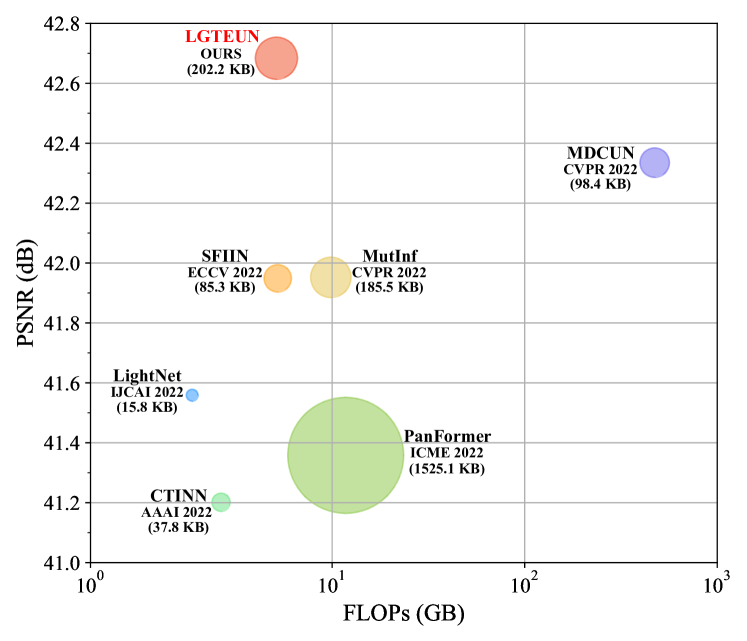
Figure 1: PSNR-Params-FLOPs comparisons between six SOTA DL-based pan-sharpening methods and our LGTEUN on the WorldView-2 satellite data set. The vertical axis is PSNR (model performance), the horizontal axis is FLOPs (computational cost), and the circle radius is Params (model complexity).

With the development of remote sensing field, multispectral (MS) image is capable of recording more abundant spectral signatures in spectral domain compared with RGB image, and is widely applied in various fields, e.g., environmental monitoring, precision agriculture, and urban development Hardie et al. (2004); Fauvel et al. (2012). However, due to the inherent trade-off between spatial and spectral resolution, it is hard to directly acquire high-resolution multispectral (HrMS) images. Pan-sharpening, a vital yet challenging remote sensing image processing task, aims to produce a HrMS image from the coupled low-resolution multispectral (LrMS) and panchromatic (PAN) images.

Formally, the degradation process of the HrMS image $\mathbf{Z}\in\mathbb{R}^{HW\times B}$ is often expressed as Hardie et al. (2004); Xie et al. (2019); Dong et al. (2021):

$$\begin{split}\mathbf{X}=\mathbf{S}\mathbf{Z}+\mathbf{N}_{x},\ \mathbf{Y}=\mathbf{Z}\mathbf{R}+\mathbf{N}_{y},\end{split}$$ (1)

where $\mathbf{S}\in\mathbb{R}^{hw\times HW}$ is a linear operator for the spatial blurring and downsampling, $\mathbf{R}\in\mathbb{R}^{B\times 1}$ is the spectral response function of the PAN imaging sensor, and $\mathbf{N}_{x}$ and $\mathbf{N}_{y}$ are the introduced noises during the image acquisition of the LrMS image $\mathbf{X}\in\mathbb{R}^{hw\times B}$ and the PAN image $\mathbf{Y}\in\mathbb{R}^{HW\times 1}$, respectively. Here, $H$ and $h$ ($H>h$), $W$ and $w$ ($W>w$), and $B$ represent the spatial height, the spatial weight, and the number of spectral bands of the corresponding image, respectively. In the past few decades, many methods have been developed in light of the degradation process in Eq. (1), which can be roughly divided into two categories, i.e., model-based and deep learning (DL)-based.

Typical model-based methods include component substitution (CS) Aiazzi et al. (2007), multiresolution analysis (MRA) Liu (2000); King and Wang (2001), and variational optimization (VO) Ballester et al. (2006); Fu et al. (2019). These methods rely on prior subjective assumptions in the super-resolving process, and show limited model performance and generalization ability in real scenes. Attracted by the impressive success of DL in various vision tasks He et al. (2016); Chollet (2017), many DL-based methods have been developed for pan-sharpening, especially convolutional neural network (CNN)-based methods. Owing to the outstanding feature representation in hierarchical manner, DL-based methods are capable of directly learning strong priors, and achieve competitive performance, e.g., PanNet Yang et al. (2017) and SDPNet Xu et al. (2020).

Model Interpretability: Despite the strong feature extraction ability and encouraging performance improvement, the weak model interpretability is a longstanding deficiency for DL-based methods due to the adopted black box principle. To this end, deep unfolding networks (DUNs) combine merits of both model-based and DL-based methods, and reasonably formulate end-to-end DL models tailored to the investigated pan-sharpening problem employing the theoretical designing philosophy. For instance, Xu et al. Xu et al. (2021) developed the first DUN for pan-sharpening, justifying the generative models for LrMS and PAN images.

Local and Global Dependencies: Although existing DUNs strengthen the model interpretability towards the investigated pan-sharpening problem, their potential has been far from fully explored. Here, for DUNs, we claim that a competitive denoiser of the image denoising step would sufficiently complement the data step in each iterative stage. However, limited by the local receptive field, most popular CNN-based denoisers pay less attention to global dependencies, which are as important as local dependencies. Furthermore, global transformer, e.g., Vision Transformer (ViT) Dosovitskiy et al. (2020), can capture global dependencies, obtaining outstanding performance in vision tasks. Yet, global transformer has nontrivial quadratic computational complexity to input image size due to the computation of global self-attention, which inescapably decreases model efficiency.

Similarly, MDCUN Yang et al. (2022) employed non-local prior and non-local block Wang et al. (2018) for modeling long-range dependencies, thus showing high computational cost. Besides DUNs, Zhou et al. Zhou et al. (2022a) proposed a modality-specific PanFormer based on Swin Transformer Liu et al. (2021). To capture local and long-range dependencies, Zhou et al. Zhou et al. (2022b) designed a CNN and transformer dual-branch model, CTINN. However, no matter the serial model, e.g., PanFormer, or the dual-branch model, e.g., CTINN, they both fail to model local and global dependencies in the same layer, which inevitably generates few limitations to the image denoiser or the total pan-sharpening model.

Following the above analysis, in this paper, we develop a transformer-based deep unfolding network, Local-Global Transformer Enhanced Unfolding Network (LGTEUN), for the interpretable MS pan-sharpening. To be specific, we first formulate a unified variational optimization problem in light of the degenerating observation of pan-sharpening, and design an iterative proximal gradient descent (PGD) algorithm to alternately solve its data and prior subproblems. Second, we elaborate a Local-Global Transformer (LGT) as a prior module for image denoising. The key component in each LGT basic block is its token mixer, the Local-Global Mixer (LG Mixer), which consists of a local branch and a global branch. The local branch calculates local window based self-attention in spatial domain, while the global branch extracts global contextual feature representation in frequency domain. Therefore, the LGT-based prior module can simultaneously capture local and global dependencies, and we also design a lightweight data module. Finally, when unfolding the iterative algorithm into the stage-wise unfolding network, LGTEUN, we serially integrate the lightweight data module and the powerful prior module in each iterative stage. Extensive experimental results on three satellite data sets demonstrate the superiority of our method compared with other state-of-the-art (SOTA) methods (as shown in Fig. 1). Our contributions can be summarized as follows:

1) We customize a transformer module LGT as an image denoiser to efficiently model local and global dependencies at the same time and sufficiently mine the potential of the proposed unfolding pan-sharpening framework.

2) We develop an interpretable transformer-based deep unfolding network, LGTEUN. To the best of our knowledge, LGTEUN is the first transformer-based deep unfolding network for the MS pan-sharpening, and LGT is also the first transformer module to perform spatial and frequency dual-domain learning.

2 Related Work

In this section, the related deep unfolding networks and transformer-based methods are briefly reviewed.

2.1 Deep Unfolding Network

Through integrating merits of both model-based and DL-based methods, deep unfolding networks (DUNs) much improve the interpretability of DL-based models. DUN unfolds the iterative algorithm tailored to the investigated problem, and optimizes the algorithm employing neural modules in an end-to-end trainable manner. DUN has been utilized to solve different low-level vision tasks, including image denoising Mou et al. (2022), image compressive sensing Zhang and Ghanem (2018), image reconstruction Cai et al. (2022), and image super-resolution Xie et al. (2019); Zhang et al. (2020); Dong et al. (2021). For the discussed MS pan-sharpening, GPPNN Xu et al. (2021) and MDCUN Yang et al. (2022) are two representative DUNs. However, restricted by the local receptive field, the adopted CNN-based denoiser in GPPNN pays less attention to global dependencies, which is adverse for reducing copy artifacts. Although MDCUN introduces non-local prior and non-local block to model long-range dependencies, the additional computational cost is heavy. Thus, it is still a crucial issue for DUN to formulate a competitive denoiser of the image denoising step to efficiently capture local and global dependencies and further sufficiently complement the data step in each iterative stage.

2.2 Transformer

Originating from language tasks Vaswani et al. (2017), transformer has an excellent ability to capture global dependencies, and has been widely applied in various vision tasks, e.g., image classification, object detection, semantic segmentation, and image restoration Dosovitskiy et al. (2020); Liu et al. (2021); Liang et al. (2021); Zhou et al. (2022a, b). However, transformer encounters two main issues. 1) Global transformer has nontrivial quadratic computation complexity to input image size due to the computation of image-level self-attention. 2) Although equipped with considerable-size windows and non-local interactions across windows, local transformer still has difficulties to model image-level global dependencies. Moreover, for pan-sharpening task, transformer-involved models, e.g., Zhou et al. (2022a) and Zhou et al. (2022b), fail to process both local and global dependencies at the same time, which inevitably limits the overall performance.

3 Method

3.1 Model Formulation and Optimization

Technically, under the maximizing a posterior (MAP) framework, recovering the original HrMS image based on the degradation process in Eq. (1) is a typical ill-posed problem. Generally, the estimation of the HrMS image $\mathbf{Z}$ is implemented by minimizing the following energy function as

$$\begin{split}\bar{\mathbf{Z}}&=\underset{\mathbf{Z}}{argmin}\frac{1}{2}{\parallel\mathbf{X}-\mathbf{S}\mathbf{Z}\parallel}^{2}+\frac{1}{2}{\parallel\mathbf{Y}-\mathbf{Z}\mathbf{R}\parallel}^{2}+\lambda J(\mathbf{Z}),\\ \end{split}$$ (2)

where $\frac{1}{2}{\parallel\mathbf{X}-\mathbf{S}\mathbf{Z}\parallel}_{2}^{2}$ and $\frac{1}{2}{\parallel\mathbf{Y}-\mathbf{Z}\mathbf{R}\parallel}_{2}^{2}$ are the two data fidelity terms coinciding with the degenerating observation, $J(\mathbf{Z})$ is the prior term to constraint the solution space, and $\lambda$ is a trade-off parameter.

Subsequently, proximal gradient descent (PGD) algorithm Beck and Teboulle (2009) is employed to solve Eq. (2) as an iterative convergence problem, i.e.,

$$\begin{split}\bar{\mathbf{Z}}_{k}&=\underset{\mathbf{Z}}{argmin}\frac{1}{2}{\parallel\mathbf{Z}-(\bar{\mathbf{Z}}_{k-1}-\eta\nabla_{f}(\bar{\mathbf{Z}}_{k-1})\parallel}^{2}+\lambda J(\mathbf{Z}),\\ \end{split}$$ (3)

where $\bar{\mathbf{Z}}_{k}$ denotes the output of the $k$-th iteration, and $\eta$ is the step size. Here, the data terms oriented differentiable operator $\nabla_{f}(\bar{\mathbf{Z}}_{k-1})$ is further calculated as

$$\begin{split}\nabla_{f}(\bar{\mathbf{Z}}_{k-1})&=\mathbf{S}^{T}(\mathbf{S}\bar{\mathbf{Z}}_{k-1}-\mathbf{X})+(\bar{\mathbf{Z}}_{k-1}\mathbf{R}-\mathbf{Y})\mathbf{R}^{T}.\\ \end{split}$$ (4)

Moreover, this iterative problem can be addressed by alternately solving its data subproblem at the gradient descent step (Eq. (5)) and its prior subproblem at the proximal mapping step (Eq. (6)). In detail,

$$\begin{split}\bar{\mathbf{Z}}_{k-\frac{1}{2}}&=\bar{\mathbf{Z}}_{k-1}-\eta\nabla(\bar{\mathbf{Z}}_{k-1}),\\ \end{split}$$ (5)

$$\begin{split}\bar{\mathbf{Z}}_{k}&=prox_{\eta,J}(\bar{\mathbf{Z}}_{k-\frac{1}{2}}),\\ \end{split}$$ (6)

where $prox_{\eta,J}$ represents the proximal operator dependent on the prior term $J(\cdot)$. In this way, the PGD algorithm utilizes a few iterations to alternately update $\bar{\mathbf{Z}}_{k-\frac{1}{2}}$ and $\bar{\mathbf{Z}}_{k}$ until convergence. In particular, from a Bayesian perspective, the solution of the prior subproblem Eq. (6) corresponds to a Gaussian denoising problem with noise level $\sqrt{\lambda}$ Chan et al. (2016); Zhang et al. (2020); Mou et al. (2022); Cai et al. (2022). In this work, we elaborate a transformer-based denoiser to approximate the proximal operator $prox_{\eta,J}$, which prominently facilitates the denoising capability and further sufficiently complements the data step in each iterative stage.

3.2 Deep Unfolding Network

Through unfolding the iterative PGD algorithm, as illustrated in Fig. 2, we develop our Local-Global Transformer Enhanced Unfolding Network (LGTEUN). The LGTEUN is comprised of several stages. Each stage contains a lightweight CNN-based data module $\mathcal{D}$ and a powerful transformer-based prior module $\mathcal{P}$, corresponding to the data subproblem at the gradient descent step (Eq. (5)) and the prior subproblem at the proximal mapping step (Eq. (6)) in each iteration, respectively.

3.2.1 Data Module $\mathcal{D}$

To approximate the closed-form solution of the data subproblem at the gradient descent step (Eq. (5)), we design a lightweight CNN-based data module, i.e.,

$$\begin{split}\bar{\mathbf{Z}}_{k-\frac{1}{2}}=\mathcal{D}(\bar{\mathbf{Z}}_{k-1},\mathbf{X},\mathbf{Y},\eta_{k-1}).\\ \end{split}$$ (7)

Specifically, as shown in Fig. 2 (a), the data module of the $k$-th stage takes the out of the $k-1$-th stage $\bar{\mathbf{Z}}_{k-1}$, the LrMS image $\mathbf{X}$, the PAN image $\mathbf{Y}$, and the stage-specific learnable step size $\eta_{k-1}$ as its module inputs. What’s more, the matrix $\mathbf{S}$ is implemented by two downsampling units, and each unit consists of a downsampling operation and a 3$\times$3 depth convolution (Conv) layer Chollet (2017). Similarly, the transposed matrix $\mathbf{S}^{T}$ is performed by two upsampling units. Besides, one point Conv Chollet (2017) is utilized as the matrix $\mathbf{R}$ to reduce channels from $B$ to $1$, and another point Conv is utilized as the matrix $\mathbf{R}^{T}$ for the corresponding inverse channel increase.

3.2.2 Prior Module $\mathcal{P}$

Considering the designing of the denoiser at the image denoising step, previous DUNs are mainly based on CNN, presenting limitations in capturing global dependencies. Here, as the first transformer-based image denoiser in the MS pan-sharpening oriented DUN, we dedicate significant efforts to craft a Local-Global Transformer (LGT) as the key denoising prior module $\mathcal{P}$, i.e.,

$$\begin{split}\bar{\mathbf{Z}}_{k}=\mathcal{P}(\bar{\mathbf{Z}}_{k-\frac{1}{2}}).\\ \end{split}$$ (8)

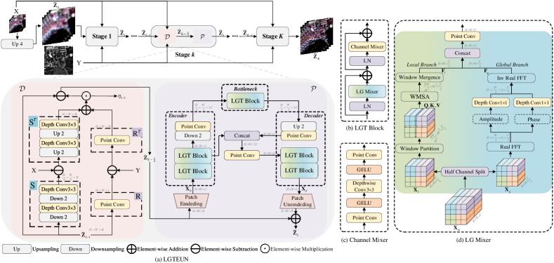
Figure 2: Illustration of the proposed LGTEUN. (a) The overall architecture of LGTEUN with $K$ stages and details of the $k$-th stage. The lightweight CNN-based data module $\mathcal{D}$ and the powerful transformer-based prior module $\mathcal{P}$ in each stage correspond to the data and prior subproblems in an iteration of the PGD algorithm. (b) Components of an LGT block. (c) The adopted channel mixer. (d) The key LG Mixer is comprised of a local branch and a global branch.

Overall Architecture of LGT.

As depicted in Eq. (8) and Fig. 2 (a), given the output $\bar{\mathbf{Z}}_{k-\frac{1}{2}}\in\mathbb{R}^{H\times W\times B}$ of $\mathcal{D}$ as the module input, LGT applies a U-shaped structure mainly constituted by a series of basic LGT Blocks, and outputs $\bar{\mathbf{Z}}_{k}\in\mathbb{R}^{H\times W\times B}$ as the module output. Concretely, LGT first uses a patch embedding layer to split the intermediate image $\bar{\mathbf{Z}}_{k-\frac{1}{2}}$ into non-overlapping patch tokens and further produces the embedded feature $\mathbf{X}_{0}\in\mathbb{R}^{H\times W\times C}$. Second, an encoder-bottleneck-decoder structure extracts the discriminative feature representation $\mathbf{X}_{d}\in\mathbb{R}^{H\times W\times C}$ from $\mathbf{X}_{0}$. In particular, the encoder and decoder both contain two LGT blocks and a resizing unit, and the bottleneck has a single LGT block. In each resizing unit, the downsampling or upsampling operation is responsible for resizing spatial resolution, and a point Conv changes the channel dimension accordingly. Finally, a patch unembedding layer is employed to project $\mathbf{X}_{d}$ to $\bar{\mathbf{Z}}_{k}$. Here, note that the patch size is set as 1, thus the original pixel vectors in $\bar{\mathbf{Z}}_{k-\frac{1}{2}}$ act as the discussed patch tokens for finer local and global token mixing.

In Fig. 2 (b), each LGT block consists of a layer normalization (LN), a Local-Global Mixer (LG Mixer) for mixing the spatial information, a LN, and a channel mixer in order. As illustrated in Fig. 2 (c), the channel mixer is a depthwise Conv Chollet (2017) based neural module for efficient channel mixing. Specifically, the LG Mixer as the token mixer is the key component in each LGT block, and Fig. 2 (d) depicts the LG Mixer of the first LG Block in the encoder. For convenience, let $\mathbf{X}_{in}\in\mathbb{R}^{H\times W\times C}$ represent the input feature map of our LG Mixer, which is further split into two equal parts $\mathbf{X}_{l}\in\mathbb{R}^{H\times W\times\frac{C}{2}}$ and $\mathbf{X}_{g}\in\mathbb{R}^{H\times W\times\frac{C}{2}}$ along the channel dimension. Then $\mathbf{X}_{l}$ and $\mathbf{X}_{g}$ are assigned to a local branch and a global branch, respectively. The local branch models local dependencies by computing local window based self-attention in spatial domain, while the global branch captures global dependencies by mining global contextual feature representation in frequency domain. By concatenating the output of the local branch $\mathbf{F}_{l}\in\mathbb{R}^{H\times W\times\frac{C}{2}}$ and that of the global branch $\mathbf{F}_{g}\in\mathbb{R}^{H\times W\times\frac{C}{2}}$, the local and global dependencies are simultaneously captured in our LG Mixer.

Local Branch.

The local branch calculates local window based multi-head self-attention (WMSA) in spatial domain. In detail, as shown in the left path of Fig. 2 (d), $\mathbf{X}_{l}$ is first partitioned into non-overlapping windows, and each window contains $M\times M$ patch tokens. Then the window-specific feature map with $\frac{HW}{M^{2}}\times M^{2}\times\frac{C}{2}$ dimension is obtained by simply reshaping. Subsequently, three feature embeddings $\mathbf{Q}$, $\mathbf{K}$, and $\mathbf{V}\in\mathbb{R}^{\frac{HW}{M^{2}}\times M^{2}\times\frac{C}{2}}$ are generated through a point Conv based linear projection. Furthermore, $\mathbf{Q}$, $\mathbf{K}$, and $\mathbf{V}$ are channel-wise divided into $h$ heads, i.e., $\mathbf{Q}=[\mathbf{Q}^{1},...,\mathbf{Q}^{h}]$, $\mathbf{K}=[\mathbf{K}^{1},...,\mathbf{K}^{h}]$, and $\mathbf{V}=[\mathbf{V}^{1},...,\mathbf{V}^{h}]$. Each head contains $d=\frac{C}{2h}$ channels, and Fig. 2 (d) only presents the circumstance with $h=1$ for simplification. More importantly, the WMSA map is computed as

$$\begin{split}\mathbf{F}^{i}_{a}=Softmax(\frac{\mathbf{Q}^{i}{\mathbf{K}^{i}}^{T}}{\sqrt{d}}+\mathbf{P}^{i})\mathbf{V}^{i},\ \ i=1,...,h,\\ \end{split}$$ (9)

where $\mathbf{P}^{i}\in\mathbb{R}^{M^{2}\times M^{2}}$ is the learnable position embedding. At last, for the feature map $\mathbf{F}_{a}$, we channel-wise concatenate its $h$ heads and spatially merge its $\frac{HW}{M^{2}}$ windows to yield the branch output $\mathbf{F}_{l}$.

Global Branch.

The global branch extracts global contextual feature representation in frequency domain based on the nature of Fourier transformation. To be specific, according to spectral convolution theorem in Fourier theory Frigo and Johnson (1998); Chi et al. (2020); Zhao et al. (2022); Zhou et al. (2022c, e), feature learning in frequency spectral domain has the image-wide receptive field by channel-wise Fourier transformation. Besides, point-wise multiplications in frequency domain correspond to convolutions in spatial domain. These properties provide vital theoretical guidances of our global branch.

Formally, 2D discrete Fourier transform (DFT) first converts $\mathbf{X}_{g}$ from spatial domain to Fourier frequency domain as the complex component $\mathcal{F}(\mathbf{X}_{g})$, i.e.,

$$\begin{split}\mathcal{F}(\mathbf{X}_{g})(u,v)&=\frac{1}{\sqrt{HW}}\sum\limits_{h=0}^{H-1}\sum\limits_{w=0}^{W-1}\mathbf{X}_{g}(h,w)e^{-j2\pi(\frac{h}{H}u+\frac{w}{W}v)},\end{split}$$ (10)

where $u$ and $v$ are frequency components. Here, $\mathcal{F}(\mathbf{X}_{g})\in\mathbb{C}^{H\times(\frac{W}{2}+1)\times\frac{C}{2}}$ is produced in light of the conjugate symmetry property of 2D DFT for our real input $\mathbf{X}_{g}$, and $\mathbb{C}$ denotes complex domain. Besides, the inverse 2D DFT is accordingly represented as $\mathcal{F}^{-1}(\cdot)$. Then based on the real part $R(\mathbf{X}_{g})$ and the imaginary part $I(\mathbf{X}_{g})$ of $\mathcal{F}(\mathbf{X}_{g})$, the amplitude component $\mathcal{A}(\mathbf{X}_{g})$ and the phase component $\mathcal{P}(\mathbf{X}_{g})$ are further expressed as

$$\begin{split}\mathcal{A}(\mathbf{X}_{g})(u,v)&=\sqrt{R^{2}(\mathbf{X}_{g})(u,v)+I^{2}(\mathbf{X}_{g})(u,v)},\end{split}$$ (11)

$$\begin{split}\mathcal{P}(\mathbf{X}_{g})(u,v)&=arctan[\frac{I(\mathbf{X}_{g})(u,v)}{R(\mathbf{X}_{g})(u,v)}].\end{split}$$ (12)

Furthermore, two independent 1$\times$1 depth Convs are utilized for feature learning in frequency domain, and the inverse 2D DFT $\mathcal{F}^{-1}(\cdot)$ is applied to recompose the feature representations of the amplitude and phase components back to spatial domain. In detail,

$$\begin{split}\mathbf{F}_{g}&=\mathcal{F}^{-1}(DConv(\mathcal{A}(\mathbf{X}_{g})),DConv(\mathcal{P}(\mathbf{X}_{g}))),\end{split}$$ (13)

where $DConv$ represents the applied 1$\times$1 depth Conv. In fact, to improve module efficiency, the 2D DFT and the inverse 2D DFT are computed by the 2D real fast Fourier transform (rFFT) and the inverse 2D rFFT, which can be implemented by torch.rfft2 and torch.irfft2 in PyTorch programming framework, respectively. The flowchart of our global branch is depicted in the right path of Fig. 2 (d).

4 Experiments

4.1 Data Sets and Evaluation Metrics

For the MS pan-sharpening, an 8-band MS data set acquired by the WorldView-3 sensor and two 4-band MS data sets acquired by WorldView-2 ² and GaoFen-2 sensors are adopted for experimental analysis. Due to the unavailability of ground-truth (GT) images for training, following Wald’s protocol Wald et al. (1997), we employ downsampling operations to produce a reduced-resolution data set for each satellite sensor. Each data set is further split into non-overlapping subsets for training (about 1000 LrMS/PAN/GT image pairs) and testing (about 140 LrMS/PAN/GT image pairs). The spatial sizes of LrMS, PAN, and GT images are $32\times 32$, $128\times 128$, and $128\times 128$, respectively. In addition, we only adopt upsampling operations to produce a full-resolution data set with 120 LrMS/PAN/GT image pairs for the WorldView-3 satellite sensor.

For image quality assessment (IQA), five popular metrics are applied for the reduced-resolution test, i.e., PSNR, SSIM, Q-index, SAM, and ERGAS, and three common non-reference metrics are employed for the full-resolution test, i.e., $D_{\lambda}$, $D_{S}$, and QNR. Besides, the inference time, parameters (Params), and floating-point operations (FLOPs) are utilized for model efficiency analysis.

Table 1: Performance and efficiency of LGTEUN with different numbers of stages $K$ on WorldView-3 and WorldView-2 satellite data sets.

Data Set	Metric	Stage 1	Stage 2	Stage 3	Stage 4
WorldView-3	PSNR$\uparrow$	32.0339	32.2188	32.068	32.0042
	SSIM$\uparrow$	0.9532	0.9545	0.9535	0.9527
	Q8$\uparrow$	0.9481	0.9494	0.9487	0.9480
	SAM$\downarrow$	0.0605	0.0605	0.0603	0.0612
	ERGAS$\downarrow$	2.6765	2.6286	2.6678	2.6898
	Time (s/img)	0.0070	0.0133	0.0205	0.0262
	Params (KB)	270.2	540.0	809.9	1079.7
	FLOPs (GB)	9.52	19.04	28.56	38.08
WorldView-2	PSNR$\uparrow$	42.600	42.6837	42.4771	42.1634
	SSIM$\uparrow$	0.9784	0.9786	0.9781	0.9767
	Q4$\uparrow$	0.8398	0.8415	0.8383	0.8329
	SAM$\downarrow$	0.0209	0.0208	0.0213	0.0222
	ERGAS$\downarrow$	0.9358	0.928	0.9573	0.9787
	Time (s/img)	0.0065	0.0137	0.0204	0.0254
	Params (KB)	101.2	202.2	303.2	404.2
	FLOPs (GB)	2.57	5.14	7.71	10.28

Table 2: Quantitative comparison of different methods on WorldView-3, WorldView-2, and GaoFen-2 satellite data sets.

Method	WorldView-3					WorldView-2					GaoFen-2
	PSNR$\uparrow$	SSIM$\uparrow$	Q8$\uparrow$	SAM$\downarrow$	ERGAS$\downarrow$	PSNR$\uparrow$	SSIM$\uparrow$	Q4$\uparrow$	SAM$\downarrow$	ERGAS$\downarrow$	PSNR$\uparrow$	SSIM$\uparrow$	Q4$\uparrow$	SAM$\downarrow$	ERGAS$\downarrow$
GSA	22.5164	0.6343	0.5742	0.1106	7.8267	33.5975	0.8899	0.5681	0.0573	2.5402	36.0557	0.8838	0.5517	0.0641	3.5758
SFIM	21.4154	0.5415	0.4525	0.1147	8.8553	32.6334	0.8728	0.5159	0.0597	3.1919	34.7715	0.8572	0.4584	0.0657	4.2073
Wavelet	21.4464	0.5656	0.5271	0.1503	9.1545	32.1992	0.8500	0.4577	0.0638	3.3799	33.9208	0.8197	0.4033	0.0695	4.6445
PanFormer	30.4772	0.9368	0.9316	0.0672	3.1830	41.3581	0.9731	0.8236	0.0241	1.0617	44.8540	0.9805	0.8865	0.0271	1.3334
CTINN	31.8564	0.9518	0.9460	0.0660	2.7421	41.2015	0.9735	0.8149	0.0246	1.0880	44.2942	0.9784	0.8716	0.0293	1.4148
LightNet	32.0018	0.9525	0.9472	0.0639	2.6853	41.5589	0.9739	0.8220	0.0237	1.0382	44.6876	0.9787	0.8741	0.0279	1.3510
SFIIN	31.6587	0.9492	0.9435	0.0652	2.8016	41.9489	0.9752	0.8108	0.0229	1.0084	44.7248	0.9802	0.8721	0.0280	1.3361
MutInf	31.8298	0.9523	0.9469	0.0636	2.7526	41.9522	0.9760	0.8258	0.0227	1.0153	44.8305	0.9800	0.8836	0.0277	1.3394
MDCUN	31.2978	0.9429	0.9363	0.0661	2.9295	42.3351	0.9772	0.8370	0.0216	0.9638	45.5677	0.9825	0.8915	0.0252	1.2249
LGTEUN	32.2188	0.9545	0.9494	0.0605	2.6286	42.6837	0.9786	0.8415	0.0208	0.9280	45.8364	0.9840	0.8973	0.0247	1.1824

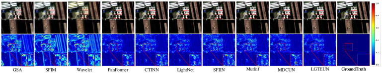
Figure 3: Qualitative comparison of different methods on the WorldView-2 satellite data set.

4.2 Implementation Details

Training Setting.

The end-to-end training of LGTEUN is supervised by mean absolute error (MAE) loss between the network output $\bar{\mathbf{Z}}_{K}$ and the GT HrMS image. It trains $130$ epochs for the 8-band data set, and $1000$ epochs for the two 4-band data sets. The Adam optimizer with $\beta_{1}=0.9$ and $\beta_{2}=0.999$ is employed for model optimization, and the batch size is set as $4$. The initial learning rate is $1.5\times 10^{-3}$, and decays by $0.85$ every $100$ epochs. All the experiments are conducted in PyTorch framework with a single NVIDIA GeForce GTX 3090 GPU. For clear comparisons, red color highlights the best results while blue color the second-best in the following suitable table results.

Structure Setting.

As shown in Fig. 2 (a), $\bar{\mathbf{Z}}_{0}$ is initialized by directly upsampling the LrMS image $\mathbf{X}$ with a scaling factor $4$. In LGTEUN, the data module $\mathcal{D}$ shares parameters across stages, while the prior module maintains independence. The channel number $C$ is set as $4B$ for all the data sets. Additionally, all the downsampling or upsampling operation is implemented by the bicubic interpolation.

Besides, in the local branch of each LGT block, the size of each local window $M$ is $8$, and the number of heads is $2$. Moreover, in Tab. 1, we explore the impact of the number of iterative stages $K=1,2,3,4$ from performance and efficiency viewpoints on 8-band WorldView-3 and 4-band WorldView-2 satellite scenes. According to the results in Tab. 1, it is clear that LGTEUN reaches the optimal performance with $2$ stages, and the model efficiency gradually decreases as $K$ increases. Hence, the number of stages is chosen as $2$ for better performance and efficiency balance.

4.3 Comparison with SOTA Methods

To comprehensively evaluate the effectiveness and efficiency of the proposed method for the MS pan-sharpening, we compare our LGTEUN with three model-based methods, i.e., GSA Aiazzi et al. (2007), SFIM Liu (2000), and Wavelet King and Wang (2001), and six SOTA DL-based methods, i.e., PamFormer Zhou et al. (2022a), CTINN Zhou et al. (2022a), LightNet Chen et al. (2022), SFIIN Zhou et al. (2022c), MutInf Zhou et al. (2022d), and MDCUN Yang et al. (2022). Besides, all the compared methods are implemented in light of the corresponding paper and source code. It is noteworthy that all the six DL-based methods are the most recent algorithms for the MS pan-sharpening.

Quantitative Comparison.

Tab. 2 reports the comparison results of all the discussed ten methods on all the three satellite data sets. Specifically, on all the three data sets, the three model-based methods show limited model performances and generalization abilities, and the DL-based methods obtain more competitive results. More importantly, among all the considered methods on all the three data sets, our proposed LGTEUN always achieves the best results in all the five IQA metrics with distinct performance improvements. For instance, our LGTEUN outperforms the second-best method by 0.2170 dB, 0.3486 dB, and 0.2687 dB in PSNR on WorldView-3, WorldView-2, and GaoFen-2 data sets, respectively, which indicates the superiority of our proposed method.

Table 3: Full-resolution test of different methods on the WorldView-3 satellite data set.

Method	Full-resolution Test
	$D_{\lambda}$$\downarrow$	$D_{S}$$\downarrow$	QNR$\uparrow$
GSA	0.0094	0.1076	0.8839
SFIM	0.0094	0.1061	0.8854
Wavelet	0.0552	0.1330	0.8193
PanFormer	0.0191	0.0416	0.9400
CTINN	0.0123	0.0442	0.9440
LightNet	0.0185	0.0282	0.9539
SFIIN	0.0198	0.0352	0.9457
MutInf	0.0163	0.0420	0.9423
MDCUN	0.0747	0.1673	0.7708
LGTEUN	0.0162	0.0310	0.9532

Table 4: Efficiency comparison of different methods on WorldView-3 and GaoFen-2 satellite data sets.

Data Set	Metric	GSA	SFIM	Wavelet	PanFormer	CTINN	LightNet	SFIIN	MutInf	MDCUN	LGTEUN
WorldView-3	Time (s/img)	0.0482	0.0591	0.0562	0.0160	0.0426	0.0019	0.0529	0.1083	0.1747	0.0133
	Params (KB)	–	–	–	1532.8	38.3	16.3	85.8	185.8	140.9	540.0
	FLOPs (GB)	–	–	–	11.92	2.68	2.02	5.25	9.87	479.54	19.04
GaoFen-2	Time (s/img)	0.0216	0.0301	0.0271	0.0257	0.0431	0.0017	0.0528	0.1141	0.1017	0.0129
	Params (KB)	–	–	–	1530.3	37.8	15.8	85.3	185.5	98.3	202.2
	FLOPs (GB)	–	–	–	11.77	2.65	1.95	5.22	9.85	473.19	5.14

Table 5: Ablation study on the WorldView-3 satellite data set.

Setting		Reduced-resolution Test					Full-resolution Test
Local Branch	Global Branch	PSNR$\uparrow$	SSIM$\uparrow$	Q8$\uparrow$	SAM$\downarrow$	ERGAS$\downarrow$	$D_{\lambda}$$\downarrow$	$D_{S}$$\downarrow$	QNR$\uparrow$
✗	✓	31.9309	0.9519	0.9468	0.0636	2.7102	0.0177	0.0364	0.9465
✓	✗	31.9742	0.9525	0.9468	0.0618	2.7029	0.0170	0.0349	0.9486
✓	✓	32.2188	0.9545	0.9494	0.0605	2.6286	0.0162	0.0310	0.9532

Qualitative Comparison.

Fig. 3 illustrates the qualitative results of a typical sample from the WorldView-2 data set, including the paired output pan-sharpening image and the corresponding MAE residual image of each discussed method. In Fig. 3, compared with the other nine methods, the proposed LGTEUN exhibits a more visually pleasing result with minor spectral and spatial distortions. In particular, the residual image of our method has fewer artifacts than any other method, especially in the zoom-in region. Here, we can reasonably infer that the advanced performance of the LGTEUN benefits from the designed PGD algorithm based stage iterations and the excellent capability of simultaneously capturing local and global dependencies.

Full-resolution Test.

To further measure the model performance in the full-resolution scene, we conduct a full-resolution test on the full-resolution WorldView-3 data set. As reported in Tab. 3, the proposed method also obtains competitive results, i.e., second-best results in $D_{S}$ and QNR and the third-best result in $D_{\lambda}$. On the contrary, MDCUN Yang et al. (2022) exhibits slightly limited results.

Efficiency Comparison.

As for efficiency comparison, Tab. 4 presents exhaustive investigations about inference efficiency (the inference time), model complexity (Params), and computational cost (FLOPs) of all the ten methods on WorldView-3 and GaoFen-2 data sets, and Fig. 1 illustrates the unified PSNR-Params-FLOPs comparisons of all the DL-based methods on the WorldView-2 scenario. Specifically, from Tab. 4, the proposed LGTEUN has excellent inference efficiency and promising computational cost. Besides, further considering the outstanding model performance in Fig. 1, our LGTEUN achieves an impressive performance-efficiency balance.

4.4 Analysis and Discussion

Ablation Study.

In this subsection, we perform an ablation study towards our elaborated LGT in the prior module $\mathcal{P}$. Specifically, on the WorldView-3 data set, two break-down ablation tests are conducted to explore and validate the corresponding contributions of its key local and global branches.

Local Branch: For one thing, the local branch models local dependencies by computing local window based self-attention in spatial domain. As reported in Tab. 5, the local branch brings obvious performance gains for both reduced-resolution and full-resolution tests. For example, our LGTEUN improves 0.2879 dB in PSNR and 0.0816 in ERGAS for the reduced-resolution test, and 0.0067 in QNR for the full-resolution test, respectively.

Global Branch: For another thing, the global branch captures global dependencies by mining global contextual feature representation in frequency domain. From Tab. 5, the importance of modeling global dependencies is self-evident since there are distinct performance degradations on all the IQA metrics without the global branch, e.g., 0.2446 dB in PSNR and 0.0026 in Q8 for the reduced-resolution test, and 0.0039 in $D_{S}$ for the full-resolution test, respectively.

Stage-wise Visualization.

As illustrated in Fig. 4, for our LGTEUN, we visualize the intermediate results of different stages ($\bar{\mathbf{Z}}_{0}$, $\bar{\mathbf{Z}}_{1}$, and $\bar{\mathbf{Z}}_{2}$) from a representative sample in the GaoFen-2 satellite data set, including the paired pan-sharpening and residual images. It is clear that more detailed information is recovered with LGTEUN iterating.

Limitations.

In short, two-fold potential limitations of our LGTEUN are as follows: 1) The pan-sharpening results on the full-resolution scene have room for performance boosting. 2) Further enhancements on model efficiency would make our proposed LGTEUN more competitive.

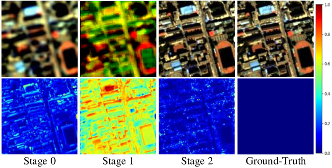
Figure 4: Stage-wise visualization on the GaoFen-2 satellite scene.

5 Conclusion

In this paper, for the MS pan-sharpening, we develop our LGTEUN by unfolding the designed PGD optimization algorithm into a deep network to improve the model interpretability. In our LGTEUN, to complement the lightweight data module, we customize a LGT module as a powerful prior module for image denoising to simultaneously capture local and global dependencies. To the best of our knowledge, LGTEUN is the first transformer-based DUN for the MS pan-sharpening, and LGT is also the first transformer module to perform spatial and frequency dual-domain learning. Comprehensive experimental results on three satellite data sets demonstrate the effectiveness and efficiency of our LGTEUN compared with other SOTA methods.

References

- Aiazzi et al. [2007] Bruno Aiazzi, Stefano Baronti, and Massimo Selva. Improving component substitution pansharpening through multivariate regression of ms pan data. IEEE Transactions on Geoscience and Remote Sensing, 45(10):3230–3239, 2007.
- Ballester et al. [2006] Coloma Ballester, Vicent Caselles, Laura Igual, Joan Verdera, and Bernard Rougé. A variational model for p+ xs image fusion. International Journal of Computer Vision, 69(1):43–58, 2006.
- Beck and Teboulle [2009] Amir Beck and Marc Teboulle. A fast iterative shrinkage-thresholding algorithm for linear inverse problems. SIAM journal on imaging sciences, 2(1):183–202, 2009.
- Cai et al. [2022] Yuanhao Cai, Jing Lin, Haoqian Wang, Xin Yuan, Henghui Ding, Yulun Zhang, Radu Timofte, and Luc Van Gool. Degradation-aware unfolding half-shuffle transformer for spectral compressive imaging. Advances in Neural Information Processing Systems, 2022.
- Chan et al. [2016] Stanley H Chan, Xiran Wang, and Omar A Elgendy. Plug-and-play admm for image restoration: Fixed-point convergence and applications. IEEE Transactions on Computational Imaging, 3(1):84–98, 2016.
- Chen et al. [2022] Zhi-Xuan Chen, Cheng Jin, Tian-Jing Zhang, Xiao Wu, and Liang-Jian Deng. Spanconv: A new convolution via spanning kernel space for lightweight pansharpening. In Proc. 31st Int. Joint Conf. Artif. Intell., pages 1–7, 2022.
- Chi et al. [2020] Lu Chi, Borui Jiang, and Yadong Mu. Fast fourier convolution. Advances in Neural Information Processing Systems, 33:4479–4488, 2020.
- Chollet [2017] François Chollet. Xception: Deep learning with depthwise separable convolutions. In Proceedings of the IEEE/CVF Conference on Computer Vision and Pattern Recognition, pages 1251–1258, 2017.
- Dong et al. [2021] Weisheng Dong, Chen Zhou, Fangfang Wu, Jinjian Wu, Guangming Shi, and Xin Li. Model-guided deep hyperspectral image super-resolution. IEEE Transactions on Image Processing, 30:5754–5768, 2021.
- Dosovitskiy et al. [2020] Alexey Dosovitskiy, Lucas Beyer, Alexander Kolesnikov, Dirk Weissenborn, Xiaohua Zhai, Thomas Unterthiner, Mostafa Dehghani, Matthias Minderer, Georg Heigold, Sylvain Gelly, et al. An image is worth 16x16 words: Transformers for image recognition at scale. In International Conference on Learning Representations, 2020.
- Fauvel et al. [2012] Mathieu Fauvel, Yuliya Tarabalka, Jon Atli Benediktsson, Jocelyn Chanussot, and James C Tilton. Advances in spectral-spatial classification of hyperspectral images. Proceedings of the IEEE, 101(3):652–675, 2012.
- Frigo and Johnson [1998] Matteo Frigo and Steven G Johnson. Fftw: An adaptive software architecture for the fft. In Proceedings of IEEE International Conference on Acoustics, Speech and Signal Processing, volume 3, pages 1381–1384, 1998.
- Fu et al. [2019] Xueyang Fu, Zihuang Lin, Yue Huang, and Xinghao Ding. A variational pan-sharpening with local gradient constraints. In Proceedings of the IEEE/CVF Conference on Computer Vision and Pattern Recognition, pages 10265–10274, 2019.
- Hardie et al. [2004] Russell C Hardie, Michael T Eismann, and Gregory L Wilson. Map estimation for hyperspectral image resolution enhancement using an auxiliary sensor. IEEE Transactions on Image Processing, 13(9):1174–1184, 2004.
- He et al. [2016] Kaiming He, Xiangyu Zhang, Shaoqing Ren, and Jian Sun. Deep residual learning for image recognition. In Proc. IEEE/CVF Conf. Comput. Vis. Pattern Recognit., pages 770–778, 2016.
- King and Wang [2001] Roger L King and Jianwen Wang. A wavelet based algorithm for pan sharpening landsat 7 imagery. In Proceedings of IEEE International Geoscience and Remote Sensing Symposium, volume 2, pages 849–851, 2001.
- Liang et al. [2021] Jingyun Liang, Jiezhang Cao, Guolei Sun, Kai Zhang, Luc Van Gool, and Radu Timofte. Swinir: Image restoration using swin transformer. In Proceedings of the IEEE/CVF International Conference on Computer Vision Workshops, pages 1833–1844, 2021.
- Liu et al. [2021] Ze Liu, Yutong Lin, Yue Cao, Han Hu, Yixuan Wei, Zheng Zhang, Stephen Lin, and Baining Guo. Swin transformer: Hierarchical vision transformer using shifted windows. In Proceedings of the IEEE/CVF International Conference on Computer Vision, pages 10012–10022, 2021.
- Liu [2000] JG Liu. Smoothing filter-based intensity modulation: A spectral preserve image fusion technique for improving spatial details. International Journal of Remote Sensing, 21(18):3461–3472, 2000.
- Mou et al. [2022] Chong Mou, Qian Wang, and Jian Zhang. Deep generalized unfolding networks for image restoration. In Proceedings of the IEEE/CVF Conference on Computer Vision and Pattern Recognition, pages 17399–17410, 2022.
- Vaswani et al. [2017] Ashish Vaswani, Noam Shazeer, Niki Parmar, Jakob Uszkoreit, Llion Jones, Aidan N Gomez, Łukasz Kaiser, and Illia Polosukhin. Attention is all you need. Advances in Neural Information Processing Systems, 30, 2017.
- Wald et al. [1997] Lucien Wald, Thierry Ranchin, and Marc Mangolini. Fusion of satellite images of different spatial resolutions: Assessing the quality of resulting images. Photogrammetric Engineering and Remote Sensing, 63(6):691–699, 1997.
- Wang et al. [2018] Xiaolong Wang, Ross Girshick, Abhinav Gupta, and Kaiming He. Non-local neural networks. In Proceedings of the IEEE/CVF Conference on Computer Vision and Pattern Recognition, pages 7794–7803, 2018.
- Xie et al. [2019] Qi Xie, Minghao Zhou, Qian Zhao, Deyu Meng, Wangmeng Zuo, and Zongben Xu. Multispectral and hyperspectral image fusion by ms/hs fusion net. In Proceedings of the IEEE/CVF Conference on Computer Vision and Pattern Recognition, pages 1585–1594, 2019.
- Xu et al. [2020] Han Xu, Jiayi Ma, Zhenfeng Shao, Hao Zhang, Junjun Jiang, and Xiaojie Guo. Sdpnet: A deep network for pan-sharpening with enhanced information representation. IEEE Transactions on Geoscience and Remote Sensing, 59(5):4120–4134, 2020.
- Xu et al. [2021] Shuang Xu, Jiangshe Zhang, Zixiang Zhao, Kai Sun, Junmin Liu, and Chunxia Zhang. Deep gradient projection networks for pan-sharpening. In Proceedings of the IEEE/CVF Conference on Computer Vision and Pattern Recognition, pages 1366–1375, 2021.
- Yang et al. [2017] Junfeng Yang, Xueyang Fu, Yuwen Hu, Yue Huang, Xinghao Ding, and John Paisley. Pannet: A deep network architecture for pan-sharpening. In Proceedings of the IEEE/CVF International Conference on Computer Vision, pages 5449–5457, 2017.
- Yang et al. [2022] Gang Yang, Man Zhou, Keyu Yan, Aiping Liu, Xueyang Fu, and Fan Wang. Memory-augmented deep conditional unfolding network for pan-sharpening. In Proceedings of the IEEE/CVF Conference on Computer Vision and Pattern Recognition, pages 1788–1797, 2022.
- Zhang and Ghanem [2018] Jian Zhang and Bernard Ghanem. Ista-net: Interpretable optimization-inspired deep network for image compressive sensing. In Proceedings of the IEEE/CVF Conference on Computer Vision and Pattern Recognition, pages 1828–1837, 2018.
- Zhang et al. [2020] Kai Zhang, Luc Van Gool, and Radu Timofte. Deep unfolding network for image super-resolution. In Proceedings of the IEEE/CVF conference on computer vision and pattern recognition, pages 3217–3226, 2020.
- Zhao et al. [2022] Xudong Zhao, Mengmeng Zhang, Ran Tao, Wei Li, Wenzhi Liao, Lianfang Tian, and Wilfried Philips. Fractional fourier image transformer for multimodal remote sensing data classification. IEEE Transactions on Neural Networks and Learning Systems, 2022.
- Zhou et al. [2022a] Huanyu Zhou, Qingjie Liu, and Yunhong Wang. Panformer: a transformer based model for pan-sharpening. IEEE international conference on multimedia and expo, 2022.
- Zhou et al. [2022b] Man Zhou, Jie Huang, Yanchi Fang, Xueyang Fu, and Aiping Liu. Pan-sharpening with customized transformer and invertible neural network. Proceedings of the AAAI Conference on Artificial Intelligence, 2022.
- Zhou et al. [2022c] Man Zhou, Jie Huang, Keyu Yan, Hu Yu, Xueyang Fu, Aiping Liu, Xian Wei, and Feng Zhao. Spatial-frequency domain information integration for pan-sharpening. In European Conference on Computer Vision, pages 274–291, 2022.
- Zhou et al. [2022d] Man Zhou, Keyu Yan, Jie Huang, Zihe Yang, Xueyang Fu, and Feng Zhao. Mutual information-driven pan-sharpening. In Proceedings of the IEEE/CVF Conference on Computer Vision and Pattern Recognition, pages 1798–1808, 2022.
- Zhou et al. [2022e] Man Zhou, Hu Yu, Jie Huang, Feng Zhao, Jinwei Gu, Chen Change Loy, Deyu Meng, and Chongyi Li. Deep fourier up-sampling. Advances in Neural Information Processing Systems, 2022.