Counterfactual Explanation with Missing Values

Abstract

Counterfactual Explanation (CE) is a post-hoc explanation method that provides a perturbation for altering the prediction result of a classifier. Users can interpret the perturbation as an “action" to obtain their desired decision results. Existing CE methods require complete information on the features of an input instance. However, we often encounter missing values in a given instance, and the previous methods do not work in such a practical situation. In this paper, we first empirically and theoretically show the risk that missing value imputation methods affect the validity of an action, as well as the features that the action suggests changing. Then, we propose a new framework of CE, named Counterfactual Explanation by Pairs of Imputation and Action (CEPIA), that enables users to obtain valid actions even with missing values and clarifies how actions are affected by imputation of the missing values. Specifically, our CEPIA provides a representative set of pairs of an imputation candidate for a given incomplete instance and its optimal action. We formulate the problem of finding such a set as a submodular maximization problem, which can be solved by a simple greedy algorithm with an approximation guarantee. Experimental results demonstrated the efficacy of our CEPIA in comparison with the baselines in the presence of missing values.

1 Introduction

Complex machine learning models (e.g., deep neural networks) have performed well in various prediction tasks, such as loan approvals and medical diagnoses. To give human users insight into such real tasks, these models need to provide not only predictions but also information on why the predictions are given and how to alter the predictions into desired one (Miller, 2019). Counterfactual Explanation (CE) (Wachter et al., 2018) is a post-hoc explanation method that provides such information. For a classifier $h\colon\mathcal{X}\to\mathcal{Y}$, a target class $y^{\ast}\in\mathcal{Y}$, and an instance $x\in\mathcal{X}$ such that $h(x)\not=y^{\ast}$, CE provides a perturbation vector $a$ that flips the prediction result into the target class, i.e., $h(x+a)=y^{\ast}$. The user can regard the perturbation $a$ as an “action" for obtaining the desired outcome $y^{\ast}$ from the classifier $h$. For that purpose, most of the existing studies solve the following optimization problem (Ustun et al., 2019):

$$a^{\ast}=\mathop{\arg\min}_{a\in\mathcal{A}}\;c(a\mid x)\;\;\text{subject to}\;h(x+a)=y^{\ast},$$ (1)

where $\mathcal{A}$ is a set of feasible actions and $c$ is a cost function that measures the required efforts of actions $a\in\mathcal{A}$. Table 1a presents an example of an optimal action $a^{\ast}$ for $x$ extracted from a logistic regression classifier $h$ on the GiveMeCredit (GMC) dataset (Kaggle, 2011). A user can obtain the desired outcome $y^{\ast}$ from $h$ by changing $x$ to $x+a^{\ast}$.

The previous studies assume that the complete information of an input instance $x$ is given. However, we often encounter a situation where $x$ includes missing values, which makes it impossible to solve the problem (1) directly (Guidotti, 2022). For example, the Pima Indians Diabetes dataset has missing values in five out of eight features (Pearson, 2006), and the GMC dataset has about 20% missing values in the feature “MonthlyIncome." These missing values arise not only when users do not know their feature values (e.g., having not taken some medical tests due to a budget (Cesa-Bianchi et al., 2011)) but also when users do not input their values on purpose (e.g., older people tend to avoid disclosing their income (Schenker et al., 2006)). In both cases, it is difficult or costly to ask users to disclose the values of missing features (Saar-Tsechansky and Provost, 2007). Thus, practical CE methods should be able to show actions without acquiring missing values (Verma et al., 2020).

A common way to handle missing values is imputation that replaces them with plausible values (Little and Rubin, 2019). In the context of CE, however, imputation often affects resulting actions. For example, for the same instance $x$ as in Table 1a, we drop the value of the feature “MonthlyIncome" ($3000) and impute it with the empirical mean ($6661), which we write for $\hat{x}$. Table 1b shows an optimal action $\hat{a}$ for the imputed instance $\hat{x}$. Compared $\hat{a}$ with the action $a^{\ast}$ before imputation, we can see the following differences:

• Quantitative: While the cost $c(\hat{a}\mid x)$ of the action $\hat{a}$ for the original instance $x$ is smaller than that of $a^{\ast}$, it is not valid for $x$, which means $h(x+\hat{a})\not=y^{\ast}$.

• Qualitative: The features to be changed by the action $\hat{a}$ are different from those of $a^{\ast}$, though $a^{\ast}$ does not include the missing feature “MonthlyIncome" and seems not to be affected by its imputation.

These results suggest the risk that imputation affects the validity and features of the resulting action (Guidotti, 2022). This risk cannot be avoided as long as we consider only a single value for imputing each missing feature. To alleviate such a risk and stably obtain good actions even with missing values, we need to take into account multiple candidates of imputation (Rubin, 1987). However, because the imputation candidates may exist infinitely or exponentially, enumerating all of them is computationally difficult and providing all the resulting actions is not interpretable for users. Therefore, we aim to efficiently select a few imputation candidates that are representative in terms of their resulting actions.

Table 1: Examples of actions on the GiveMeCredit dataset. “Features" and “Values" indicate actions $a$. “Cost" and “Valid" indicate $c(a\mid x)$ and $h(x+a)=y^{\ast}$, respectively.

Features	Values	Cost	Valid
#30-59DaysPastDueNotWorse	$-1$	1.88	True

(a) Optimal action $a^{\ast}$ without missing values

Features	Values	Cost	Valid
RevolvingUtilizationOfU.L.	$-0.017$	1.37	False
#OpenCreditLines&Loans	$-6$

(b) Optimal action $\hat{a}$ after missing value imputation

1.1 Our Contributions

In this paper, we propose the first natural extension of CE that works even in the presence of missing values, named Counterfactual Explanation by Pairs of Imputation and Action (CEPIA). For an incomplete instance $\tilde{x}$, our CEPIA provides a representative set $\mathcal{S}$ of pairs $(\hat{x},\hat{a})$ of an imputation candidate $\hat{x}\in\mathcal{X}$ for $\tilde{x}$ and an optimal action $\hat{a}\in\mathcal{A}$ for $\hat{x}$. We formulate the task of finding such a set $\mathcal{S}$ so that it includes at least one valid action with a low cost at high probability whatever the values of missing features in $\tilde{x}$ are. We also show that our task can be formulated as a submodular maximization problem, which can be efficiently solved with an approximation guarantee (Nemhauser et al., 1978). Our contributions are summarized as follows:

1. We are the first to tackle the problem of local explanation with missing values, particularly CE. We empirically and theoretically show the risk that the resulting action is highly affected by imputation methods.

2. We propose a new framework of CE, named CEPIA, that provides a set of imputation-action pairs for a given instance with missing values. We introduce the problem of finding such a set and formulate it as a submodular maximization problem. We also show some theoretical properties of our problem.

3. We conducted experiments on public datasets and demonstrated that our CEPIA provides instances including missing values with quantitatively and qualitatively better actions than existing CE methods.

Table 2c presents an example of our CEPIA on the GMC dataset. For a given incomplete instance $\tilde{x}$ where the feature “MonthlyIncome" is missing, CEPIA outputted a set of a few imputation-action pairs $(\hat{x},\hat{a})$ with a region where each action $\hat{a}$ is estimated to be valid with the minimum cost among $\mathcal{S}$. Table 2c shows that our CEPIA provided the optimal action $a^{\ast}$ of the original instance $x$ in Table 2c even though the input $\tilde{x}$ includes missing values. If the user knows the true value of the missing feature and avoids inputting it on purpose, one can obtain the optimal action from $\mathcal{S}$ without disclosing the missing feature. As a byproduct, Table 2c also provides an overview of how the actions $\hat{a}$ are affected by imputation $\hat{x}$, which is helpful to clarify the impact of missing features on CE (Hancox-Li, 2020; Guidotti, 2022).

Table 2: An example of our CEPIA on the GiveMeCredit dataset. Each table indicates an imputation-action pair $(\hat{x},\hat{a})\in\mathcal{S}$. “Features" and “Values" for “Imputation" (resp. “Action") indicate an imputation candidate $\hat{x}$ (resp. its optimal action $\hat{a}$). Each range near to “Values" of $\hat{x}$ indicates the region where $\hat{a}$ is estimated to be valid with the minimum cost among $\mathcal{S}$.

	Features	Values
Imputation	MonthlyIncome	0 (0, 0)
Action	#30-59DaysPastDueNotWorse	$-1$
	#OpenCreditLines&Loans	$-1$

(a) Pair 1 (Cost is 2.10 and Valid is True)

	Features	Values
Imputation	MonthlyIncome	8227 (8227, 10750)
Action	#OpenCreditLines&Loans	$-4$

(b) Pair 2 (Cost is 0.79 and Valid is False)

	Features	Values
Imputation	MonthlyIncome	3471 (553, 5831)
Action	#30-59DaysPastDueNotWorse	$-1$

(c) Pair 3 (Cost is 1.88 and Valid is True)

1.2 Related Work

Counterfactual Explanation (CE), also referred to as Algorithmic Recourse, is one of the post-hoc local explanation methods that have attracted increasing attention in recent years (Verma et al., 2020). Most of the existing CE methods can be categorized depending on their optimization methods; gradient-based (Wachter et al., 2018; Mothilal et al., 2020; Lucic et al., 2022), integer optimization (Ustun et al., 2019; Kanamori et al., 2020; Parmentier and Vidal, 2021), autoencoders (Pawelczyk et al., 2020; Ley et al., 2022), or SAT (Karimi et al., 2020a; Marques-Silva et al., 2021).

While several CE methods have been proposed, recent studies pointed out various issues, e.g., causality (Karimi et al., 2020b, 2021), fairness (von Kügelgen et al., 2022), transparency (Rawal and Lakkaraju, 2020; Kanamori et al., 2022), and so on (Barocas et al., 2020; Venkatasubramanian and Alfano, 2020). One of the critical problems is robustness to the perturbations of features (Slack et al., 2021; Dominguez-Olmedo et al., 2022; Dutta et al., 2022). These studies are motivated by the fact that actions are often affected by small changes to inputs, which is similar to our observation that actions are affected by imputation. Although the existing robust CE methods can be applied to the setting with missing values if we define its uncertainty set as a sample of imputation candidates, the resulting action often has a high cost (Pawelczyk et al., 2022b) as shown in our experiments. Furthermore, since these methods provide only a single action, they cannot show the effect of imputation on actions.

Missing data analysis is a traditional branch of statistics because real datasets often contain missing values (Rubin, 1976; Little and Rubin, 2019). In the literature on machine learning, there are several studies not only on imputation with deep generative models (Yoon et al., 2018; Mattei and Frellsen, 2019), but also on the impacts of missing values and imputation on prediction consistency (Josse et al., 2019; Le Morvan et al., 2021; Ayme et al., 2022) and predictive fairness (Zhang and Long, 2021; Jeong et al., 2022). However, there is little work that studies their impacts on explanation methods, including CE, while its importance has been recognized (Ahmad et al., 2019; Verma et al., 2020; Guidotti, 2022). To the best of our knowledge, our work is the first to point out the issues with missing values for CE and propose a concrete method for addressing these issues.

2 Preliminaries

For a positive integer $n\in\mathbb{N}$, we write $[n]\coloneqq\{1,\dots,n\}$. Throughout this paper, we consider a binary classification problem as a prediction task. We denote input and output domains $\mathcal{X}=\mathcal{X}_{1}\times\dots\times\mathcal{X}_{D}\subseteq\mathbb{R}^{D}$ and $\mathcal{Y}=\{-1,+1\}$, respectively. We call a vector $x=(x_{1},\dots,x_{D})\in\mathcal{X}$ an instance, and a function $h\colon\mathcal{X}\to\mathcal{Y}$ a classifier. Without loss of generality, we assume that $h(x)=+1$ is a desirable prediction result for users (e.g., low risk of default).

2.1 Counterfactual Explanation

For an instance $x\in\mathcal{X}$, we define an action as a perturbation vector $a\in\mathbb{R}^{D}$ such that $x+a\in\mathcal{X}$. As with the existing methods (Ustun et al., 2019), we assume that we are given a set of feasible actions $\mathcal{A}(x)$ such that $\bm{0}\in\mathcal{A}(x)$ and $\mathcal{A}(x)\subseteq\{a\in\mathbb{R}^{D}\mid x+a\in\mathcal{X}\}$. For a classifier $h$, an action $a$ is valid for $x$ if $a\in\mathcal{A}(x)$ and $h(x+a)=+1$.

For an instance $x\in\mathcal{X}$ and an action $a\in\mathcal{A}(x)\subseteq\mathbb{R}^{D}$, a cost function $c\colon\mathcal{X}\times\mathbb{R}^{D}\to\mathbb{R}_{\geq 0}$ measures the required effort of $a$ with respect to $x$. Several useful cost functions, such as the $\ell_{1}$-norm weighted by the median absolute deviation (MAD) (Wachter et al., 2018) and the total-log percentile shift (TLPS) (Ustun et al., 2019), have been proposed. Throughout this paper, we assume $c(\bm{0}\mid x)=0$.

For a given classifier $h\colon\mathcal{X}\to\mathcal{Y}$ and an instance $x\in\mathcal{X}$, the aim of Counterfactual Explanation (CE) is to find an action $a$ that is valid for $x$ with respect to $h$ and minimizes its cost $c(a\mid x)$. This task can be formulated as follows:

$$\mathop{\text{minimize}}_{a\in\mathcal{A}(x)}\;c(a\mid x)\;\;\;\text{subject to}\;\;h(x+a)=+1.$$ (2)

Hereafter, we fix $h$ and $c$ and omit them if it is clear from the context. We assume that we have an oracle for solving the problem (2) and denote an optimal solution for $x$ by $a^{\ast}(x)$. Note that our framework presented later can be applied to any $h$ and $c$, and we can use any existing CE method for calculating $a^{\ast}(x)$ (e.g., (Wachter et al., 2018; Ustun et al., 2019; Pawelczyk et al., 2020; Karimi et al., 2020b)).

2.2 Missing Values

In practice, an input instance may contain features with missing values. Let $*$ be a symbol for indicating a missing value. For an original complete instance $x\in\mathcal{X}$, we denote its incomplete instance by $\tilde{x}=(\tilde{x}_{1},\dots,\tilde{x}_{D})$, where

$$\tilde{x}_{d}=\begin{cases}*,&\text{if the feature }d\text{ is missing},\\ x_{d},&\text{otherwise},\end{cases}$$

for $d\in[D]$. Let $M(\tilde{x})=\{d\in[D]\mid\tilde{x}_{d}=*\}$ (resp. $O(\tilde{x})=[D]\setminus M(\tilde{x})$) be the set of features that are missing (resp. not missing). We denote an input domain with missing values $\tilde{\mathcal{X}}=(\mathcal{X}_{1}\cup\{*\})\times\dots\times(\mathcal{X}_{D}\cup\{*\})$.

Most classifiers $h$ cannot directly handle incomplete instances $\tilde{x}\in\tilde{\mathcal{X}}$ with missing values. A common solution for this issue is imputation that replaces the missing values $*$ with plausible values and obtains imputed instances $\hat{x}\in\mathcal{X}$. There exist several practical imputation methods, such as multiple imputation by chained equations (MICE) (van Buuren and Groothuis-Oudshoorn, 2011) and $k$-nearest neighbor ($k$-NN) imputation (Troyanskaya et al., 2001).

In statistics, mechanisms of missing values are categorized into three types depending on the relationship between $M(\tilde{x})$ and $O(\tilde{x})$ (Rubin, 1976): (1) missing completely at random (MCAR) if $M(\tilde{x})$ is independent of $[D]$, (2) missing at random (MAR) if $M(\tilde{x})$ depends only on $O(\tilde{x})$, and (3) missing not at random (MNAR) if neither MCAR nor MAR holds. Note that existing methods for missing data analysis often rely on the MAR or MCAR assumption for their soundness (Little and Rubin, 2019). In our experiments, we evaluated the efficacy of our method in each situation.

3 Proposed Framework

Let us consider the situation where we have an input $\tilde{x}\in\tilde{\mathcal{X}}$ with missing values that comes from the original complete instance $x\in\mathcal{X}$ and we cannot access $x$. Using $\tilde{x}$ instead of $x$, we intend to obtain a valid action $a$ with a low cost for $x$. Since we cannot evaluate the cost $c(a\mid x)$ and prediction result $h(x+a)$, it is difficult to solve the problem (2). In this section, we first consider a naive imputation-based approach and analyze its risk by showing its theoretical properties. Motivated by these results, we introduce our approach. All the proofs of the statements are presented in Appendix.

3.1 Naive Approach and Its Drawback

A naive approach is to obtain an imputed instance $\hat{x}$ by applying an imputation method to $\tilde{x}$, and then optimize an action by solving the problem (2) for $\hat{x}$. We show theoretical relationships between optimal actions $a^{\ast}(x)$ for an original instance $x$ and $a^{\ast}(\hat{x})$ for the imputed instance $\hat{x}$. Firstly, we show two trivial properties on the validity of $a^{\ast}(\hat{x})$ for $x$:

Remark 1.

If $c(a^{\ast}(\hat{x})\mid x)<c(a^{\ast}(x)\mid x)$, then $a^{\ast}(\hat{x})$ is not valid for $x$, i.e., $a^{\ast}(\hat{x})\not\in\mathcal{A}(x)$ or $h(x+a^{\ast}(\hat{x}))\not=+1$.

Remark 2.

If $h(x)=-1$ and $h(\hat{x})=+1$, then $a^{\ast}(\hat{x})=\bm{0}$ and $a^{\ast}(\hat{x})$ is not valid for $x$ since $h(x+a^{\ast}(\hat{x}))\not=+1$.

Remark 1 implies that an optimal action $a^{\ast}(\hat{x})$ for an imputed instance $\hat{x}$ is not valid for its original instance $x$ if the cost of $a^{\ast}(\hat{x})$ is less than that of $a^{\ast}(x)$, as demonstrated in Table 1b. Remark 2 implies that if the prediction result is changed to the desired class by the imputation, $a^{\ast}(\hat{x})$ is not valid for $x$. These results indicate the risk that imputation of missing values makes optimal actions invalid.

Next, we analyze how much an optimal action $a^{\ast}(\hat{x})$ after imputation differs from $a^{\ast}(x)$. We consider the same setting as (Ustun et al., 2019). Let $h_{\beta}$ be a classifier $h_{\beta}(x)=\operatorname{sgn}(f_{\beta}(x))$ with a linear decision function $f_{\beta}(x)=\beta^{\top}x$ and a parameter $\beta\in\mathbb{R}^{D}$. We assume $\mathcal{X}=\mathbb{R}^{D}$, $\mathcal{A}(x)=\mathbb{R}^{D}$ for any $x\in\mathcal{X}$, and $c(a\mid x)=c_{x}\cdot\|a\|$, where $c_{x}>0$ is a constant depending on $x$. Furthermore, we assume that a single feature $d^{\circ}\in[D]$ is missing and that the missing value of $d^{\circ}$ is imputed with the population mean $\mu_{d^{\circ}}=\mathbb{E}_{x}\left[x_{d^{\circ}}\right]$ over a distribution $\mathcal{D}_{X}$ on the input domain $\mathcal{X}$. Note that these assumptions are common in analyses with missing values (Little and Rubin, 2019; Bertsimas et al., 2021; Josse et al., 2019). In Theorem 1, we give an upper bound on the expected difference between $a^{\ast}(x)$ and $a^{\ast}(\hat{x})$.

Theorem 1.

For an instance $x\in\mathcal{X}$ and a feature $d^{\circ}\in[D]$, we denote its imputed instance $\hat{x}\in\mathcal{X}$ with $\hat{x}_{d^{\circ}}=\mu_{d^{\circ}}$ and $\hat{x}_{d}=x_{d}$ for $d\in[D]\setminus\{d^{\circ}\}$. Then, we have

$$\mathbb{E}_{x}\left[\|a^{\ast}(\hat{x})-a^{\ast}(x)\|_{2}^{2}\right]\leq\frac{1}{\|\beta\|_{2}^{2}}\left(\beta_{d^{\circ}}^{2}\cdot\sigma_{d^{\circ}}^{2}+\gamma\cdot p_{\mathrm{conf}}\right),$$

where $\sigma_{d^{\circ}}^{2}=\mathbb{E}_{x}[(x_{d^{\circ}}-\mu_{d^{\circ}})^{2}]$, $\gamma=\mathbb{E}_{x}[\left(f_{\beta}(x)\right)^{2}\mid h_{\beta}(x)\not=h_{\beta}(\hat{x})]$, and $p_{\mathrm{conf}}=\mathbb{P}_{x}[h_{\beta}(x)\not=h_{\beta}(\hat{x})]$.

Theorem 1 implies that an upper bound on the expected difference between $a^{\ast}(x)$ and $a^{\ast}(\hat{x})$ depends on the variance $\sigma_{d^{\circ}}^{2}$ of a missing feature $d^{\circ}$ and the probability $p_{\mathrm{conf}}$ that the prediction result $h_{\beta}(x)$ is changed by imputation. This result suggests the risk that the resulting action $a^{\ast}(\hat{x})$ would be far from $a^{\ast}(x)$ even if we impute missing values with the population mean. Moreover, features included in the resulting action may be changed by imputation, as demonstrated in Table 1b. To avoid these risks, we incorporate the idea of multiple imputation (Rubin, 1987), which considers multiple ways of plausible imputation, into CE.

3.2 Our Approach

We introduce our framework, named Counterfactual Explanation by Pairs of Imputation and Actions (CEPIA). For a given incomplete instance $\tilde{x}\in\tilde{\mathcal{X}}$, our CEPIA provides a set $\mathcal{S}$ of imputation-action pairs $(\hat{x},\hat{a})$, where $\hat{x}\in\mathcal{X}$ is an imputation candidate for $\tilde{x}$ and $\hat{a}\in\mathcal{A}(\hat{x})$ is an optimal action for $\hat{x}$, i.e., $\hat{a}=a^{\ast}(\hat{x})$. Our aim is to obtain a set $\mathcal{S}$ of representative pairs $(\hat{x},\hat{a})$ so that it includes at least one action $\hat{a}$ that is quantitatively and qualitatively close to an optimal action $a^{\ast}(x)$ for $x$ at high probability. In the following, we formulate the task of obtaining such a desirable set $\mathcal{S}$ and discuss how to solve the formulated task efficiently.

3.2.1 Problem Formulation

For a given incomplete instance $\tilde{x}$, we define the set of plausible imputation candidates for $\tilde{x}$ as $\mathcal{I}(\tilde{x})\coloneqq\mathcal{I}_{1}(\tilde{x})\times\dots\times\mathcal{I}_{D}(\tilde{x})\subseteq\mathcal{X}$, where

$$\mathcal{I}_{d}(\tilde{x})\coloneqq\begin{cases}\mathcal{X}_{d}&\text{if }\tilde{x}_{d}=*,\\ \{\tilde{x}_{d}\}&\text{otherwise},\end{cases}$$

for $d\in[D]$. We call $\mathcal{I}(\tilde{x})$ the imputation space of $\tilde{x}$. By definition, the imputation space $\mathcal{I}(\tilde{x})$ includes the original instance $x$. We also define the ground set of imputation-action pairs as $\mathcal{V}(\tilde{x})\coloneqq\{(\hat{x},\hat{a})\mid\hat{x}\in\mathcal{I}(\tilde{x}),\hat{a}=a^{\ast}(\hat{x})\}$. Then, our task can be regarded as extracting a subset $\mathcal{S}$ from the ground set $\mathcal{V}(\tilde{x})$ so that it satisfies some requirements.

One ideal requirement for a set $\mathcal{S}$ is to include an optimal action $a^{\ast}(x)$ for $x$. By definition, our ground set $\mathcal{V}(\tilde{x})$ is guaranteed to include $(x,a^{\ast}(x))$. However, identifying the pair is difficult since we are given an incomplete instance $\tilde{x}$ instead of $x$. By relaxing this requirement, we aim to find $\mathcal{S}$ satisfying the following three desiderata: (1) validity: including at least one valid action for $x$ with high probability, (2) low-cost: including a valid action for $x$ whose cost is comparable with that of $a^{\ast}(x)$, and (3) interpretability: consisting of a few imputation-action pairs. To qualify the desiderata (1) and (2), we define a loss function $l$ by

$$l(x;\mathcal{S})\coloneqq\begin{cases}\min_{\hat{a}\in\mathcal{S}(x)}c(\hat{a}\mid x)&\text{if }|\mathcal{S}(x)|>0,\\ C&\text{otherwise},\end{cases}$$

where $\mathcal{S}(x)\coloneqq\{\hat{a}\in\mathcal{A}(x)\mid(\hat{x},\hat{a})\in\mathcal{S}\land h(x+\hat{a})=+1\}$ is the set of valid actions for $x$ in $\mathcal{S}$ and $C>0$ is an upper bound on the cost function $c$. If $\mathcal{S}$ includes at least one valid action for $x$, then $\mathcal{S}$ incurs the minimum cost among its valid actions; otherwise, $\mathcal{S}$ incurs the constant $C$ as its cost. For the desideratum (3), we impose the cardinality constraint $|\mathcal{S}|\leq k$ for a given size parameter $k>0$.

Since we do not have an access to $x$, we instead evaluate the loss $l$ for imputation candidates $\hat{x}\in\mathcal{I}(\tilde{x})$, and minimize the expected loss $L(\mathcal{S})\coloneqq\mathbb{E}_{\hat{x}\sim\mathcal{D}_{I}}[l(\hat{x};\mathcal{S})]$ over a distribution $\mathcal{D}_{I}$ on the imputation space $\mathcal{I}(\tilde{x})$. This idea is inspired by “Rubin’s rules" in the framework of multiple imputation (Rubin, 1987), which generates multiple imputed datasets and averages their analysis results (Dick et al., 2008; Ipsen et al., 2022). Then, we consider the following problem:

$${\mathop{\text{minimize}}}_{\mathcal{S}\subset\mathcal{V}(\tilde{x})}\;L(\mathcal{S})\;\;\;\text{subject to}\;\;|\mathcal{S}|\leq k.$$ (3)

For simplicity, we employ the uniform distribution as $\mathcal{D}_{I}$. Note that our framework can be extended to any distribution $\mathcal{D}_{I}$ if we can estimate it in advance (Little and Rubin, 2019).

Unfortunately, each of evaluating $L(\mathcal{S})$ for a fixed $\mathcal{S}$ and minimizing it with $|\mathcal{S}|\leq k$ is intractable. This is because $\mathcal{I}(\tilde{x})$ and $\mathcal{V}(\tilde{x})$ are infinite sets if the missing features are real-valued and exponentially large finite sets even if they are categorical. To alleviate this difficulty and obtain a set $\mathcal{S}$ efficiently, we take the following two steps: (i) define a surrogate problem for the problem (3) by sampling imputation candidates over $\mathcal{I}(\tilde{x})$; (ii) reformulate the problem as submodular maximization and solve it by a greedy algorithm.

3.2.2 Imputation Sampling

We first take an i.i.d. sample of $N$ imputation candidates $\hat{\mathcal{I}}(\tilde{x})=\{\hat{x}^{(1)},\dots,\hat{x}^{(N)}\}$ from $\mathcal{D}_{I}$. Next, we replace the expected loss $L(\mathcal{S})$ and ground set $\mathcal{V}(\tilde{x})$ in (3) with the empirical average $\hat{L}(\mathcal{S})\coloneqq\frac{1}{N}\sum_{n=1}^{N}l(\hat{x}^{(n)};\mathcal{S})$ over $\hat{\mathcal{I}}(\tilde{x})$ and $\hat{\mathcal{V}}(\tilde{x})\coloneqq\{(\hat{x}^{(n)},\hat{a}^{(n)})\mid\hat{a}^{(n)}=a^{\ast}(\hat{x}^{(n)})\}_{n=1}^{N}$, respectively. By minimizing $\hat{L}$, we are expected to obtain a representative subset of $\hat{\mathcal{V}}(\tilde{x})$ as with the $k$-medoids problem (Badanidiyuru et al., 2014). Then, our task can be formulated as

$${\mathop{\text{minimize}}}_{\mathcal{S}\subset\hat{\mathcal{V}}(\tilde{x})}\;\hat{L}(\mathcal{S})\;\;\;\text{subject to}\;\;|\mathcal{S}|\leq k.$$ (4)

Note that $\hat{\mathcal{I}}(\tilde{x})$ does not necessarily include the original instance $x$. To guarantee that we can obtain at least one imputation candidate $\hat{x}$ near to $x$ with high probability, we give a lower bound on the sampling size $N$ in Theorem 2.

Theorem 2.

We assume that the input domain of each feature $d\in[D]$ is bounded with a same width $w>0$, i.e., $\mathcal{X}_{d}=[l_{d},u_{d}]$ and $w=u_{d}-l_{d}$. For an incomplete instance $\tilde{x}\in\tilde{\mathcal{X}}$, let $\hat{\mathcal{I}}(\tilde{x})$ be a set of $N$ i.i.d. imputation candidates sampled from the uniform distribution $\mathcal{D}_{I}$. Then, for any $\varepsilon,\delta>0$, there exists $\hat{x}\in\hat{\mathcal{I}}(\tilde{x})$ such that $\|\hat{x}-x\|_{\infty}\leq\varepsilon$ with probability at least $1-\delta$ if $N\geq\log\frac{1}{\delta}\cdot\left(\frac{w}{2\cdot\varepsilon}\right)^{\tilde{D}}$, where $\tilde{D}=|M(\tilde{x})|$ is the total number of missing features.

3.2.3 Submodular Maximization Reformulation

While evaluating $\hat{L}(\mathcal{S})$ is tractable, the problem (4) is combinatorial optimization, which is hard to solve exactly. To address this issue, we show that the problem (4) can be formulated as a submodular maximization problem. For that purpose, we define an objective function $g\colon 2^{\hat{\mathcal{V}}(\tilde{x})}\to\mathbb{R}$ by

$$g(\mathcal{S})\coloneqq C-\hat{L}(\mathcal{S}).$$

Since $C$ is a constant, minimizing $\hat{L}(\mathcal{S})$ is equivalent to maximizing $g(\mathcal{S})$ over $\mathcal{S}\subset\hat{\mathcal{V}}(\tilde{x})$. Therefore, we can reformulate our task as the following optimization problem.

Problem 1.

Given an instance $\tilde{x}\in\tilde{\mathcal{X}}$ with missing values, a set of $N$ imputation candidates $\hat{\mathcal{I}}(\tilde{x})$, and a size parameter $k>0$, find an optimal solution to the following problem:

$${\mathop{\text{maximize}}}_{\mathcal{S}\subset\hat{\mathcal{V}}(\tilde{x})}\;g(\mathcal{S})\;\;\;\text{subject to}\;\;|\mathcal{S}|\leq k.$$

The following theorem shows that our objective function $g$ has good theoretical properties.

Theorem 3.

The objective function $g$ of Problem 1 is non-negative, monotone, and submodular over $2^{\hat{\mathcal{V}}(\tilde{x})}$.

By Theorem 3, we find that Problem 1 is a non-negative monotone submodular maximization problem with a cardinality constraint. Thus, we can efficiently solve Problem 1 by a standard greedy algorithm with a $(1-\frac{1}{e})$-approximation guarantee (Nemhauser et al., 1978).

Finally, we show that the difference between the expected loss $L$ of an approximate solution to Problem 1 and the optimal value of the problem (3) is bounded with high probability through a PAC-style bound (Mohri et al., 2012).

Theorem 4.

For $\tilde{x}\in\tilde{\mathcal{X}}$ and $\alpha\in[0,1]$, let $\mathcal{S}^{\ast}$ and $\mathcal{S}_{\alpha}$ be an optimal solution to the problem (3) and $\alpha$-approximation solution to Problem 1 such that $g(\mathcal{S}_{\alpha})\geq\alpha\cdot g^{\ast}$ for the optimal value $g^{\ast}$ of Problem 1, respectively. Then, for any $\delta>0$, the following inequality holds with probability $1-\delta$:

$$L(\mathcal{S}_{\alpha})-L(\mathcal{S}^{\ast})\leq\gamma_{\mathrm{bias}}+\gamma_{\mathrm{var}}+\gamma_{\mathrm{approx}},$$

where $\gamma_{\mathrm{bias}}=\min_{\mathcal{S}\subset\hat{\mathcal{V}}(\tilde{x}):|\mathcal{S}|\leq k}L(\mathcal{S})-L(\mathcal{S}^{\ast})$, $\gamma_{\mathrm{var}}=C\cdot\sqrt{(2/N)\cdot(k\cdot\ln N+\ln(2/\delta))}$, and $\gamma_{\mathrm{approx}}=C\cdot(1-\alpha)$.

Optimization.

For a given incomplete instance $\tilde{x}$, our CEPIA provides $\mathcal{S}$ by solving Problem 1. In practice, we observed that its computational time mainly depended on that to obtain the ground set $\hat{\mathcal{V}}(\tilde{x})$, i.e., to calculate $a^{\ast}(\hat{x})$ for each $\hat{x}\in\hat{\mathcal{I}}(\tilde{x})$. To reduce the total number of calculating $a^{\ast}(\hat{x})$, we employ SampleGreedy algorithm (Harshaw et al., 2022), which is a variant of the greedy algorithm combined with subsampling of a ground set and has a $1/2$-approximation guarantee. The details are presented in Appendix. We also note that we can calculate each element $(\hat{x},a^{\ast}(\hat{x}))$ of the ground set $\hat{\mathcal{V}}(\tilde{x})$ in parallel.

Post-processing.

In Appendix, we propose a post-processing method that estimates a region $r\subset\mathcal{X}$ where each action $\hat{a}$ is valid with the lowest cost among $\mathcal{S}$. If users avoided inputting the true values of some features on purpose, users might determine adequate actions from $\mathcal{S}$ by comparing their true values to the given estimated regions themselves. Furthermore, even if users do not know the true values, the estimated regions give us insight into the priority of the missing features to be measured (Saar-Tsechansky and Provost, 2007), which is demonstrated in our experiments.

4 Experiments

To investigate the performance of our CEPIA, we conducted numerical experiments on public datasets. The code was implemented in Python 3.7 with scikit-learn 1.0.2 and Gurobi 9.5.1. The experiments were conducted on Ubuntu 20.04 with Intel Xeon E-2274G 4.0 GHz CPU and 32 GB memory. Owing to page limitations, the implementation details and the complete experimental results are shown in Appendix.

4.1 Experimental Settings

We randomly split each dataset into train (75%) and test (25%) instances, and trained $\ell_{2}$-regularized logistic regression classifiers (LR), two-layer ReLU network classifiers (MLP) with $30$ neurons, and random forest classifiers (RF) with $50$ decision trees as $h$ on each training dataset. For each classifier, we used existing CE methods based on integer optimization to calculate $a^{\ast}(x)$ (e.g., (Ustun et al., 2019)). As a cost function $c$, we employed MAD (Wachter et al., 2018) and TLPS (Ustun et al., 2019), which are norm-based and percentile-based cost functions, respectively. Owing to page limitations, we report the results on TLPS here. To simulate the situation where instances include missing values, for test instances $x$ with the undesired prediction results $h(x)=-1$ (e.g., “high risk of default"), we generated its incomplete instances $\tilde{x}$ by dropping their values of some features. Then, we extracted actions for $\tilde{x}$ by baseline methods and our method. We set the parameters of our method as $k=4$ and $N=100$ for its interpretability and efficiency. Sensitivity analyses of $k$ and $N$ are presented in Appendix.

Comparison baselines.

To the best of our knowledge, no existing CE method directly works with missing values. Thus, we extend existing CE methods to deal with our setting and compare our CEPIA with the following two baselines. One baseline is ImputationCE, which first obtains an imputed instance by an existing imputation method and then optimizes an action for the imputed instance. For imputation, we used the mean imputation, $k$-NN imputation (Troyanskaya et al., 2001), and MICE (van Buuren and Groothuis-Oudshoorn, 2011). We report the results of MICE here because the performances of these methods were almost similar. The other baseline is RobustCE (Dominguez-Olmedo et al., 2022), which originally optimizes a robust action with an uncertainty set of a given instance. As the uncertainty set, we employed a set $\hat{\mathcal{I}}(\tilde{x})$ of $N$ imputation candidates sampled over the imputation space ${\mathcal{I}}(\tilde{x})$.

Evaluation criteria.

To compare the performance of our method with the baselines, we measured the valid ratio, which is the ratio that the obtained actions $a$ are valid for original instances $x$ (i.e., $h(x+a)=+1$), the average cost $c(a\mid x)$, and the average computational time for each instance. We also measured the sign agreement score (Krishna et al., 2022) to evaluate the qualitative similarity to the optimal actions without missing values.

4.2 Experimental Results

4.2.1 Comparison under MCAR Situation

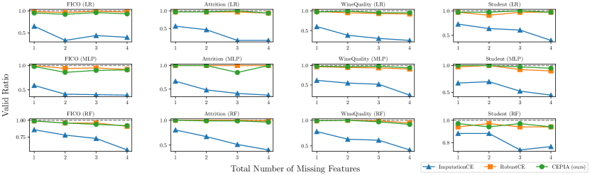
Figure 1: Experimental results of the valid ratio. The dashed lines indicate 100% validity.

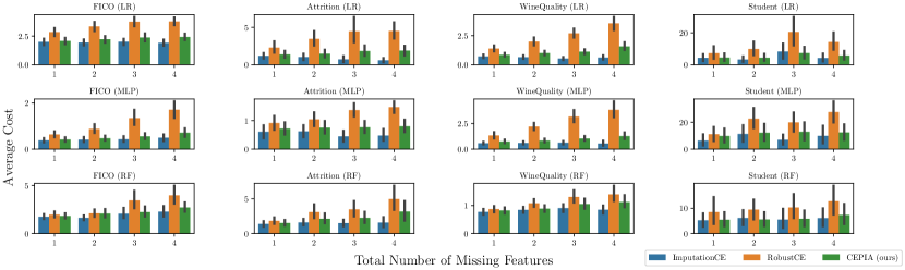
Figure 2: Experimental results of the average cost with 95% confidence intervals.

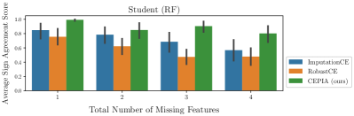
Figure 3: Experimental results of the average sign agreement score for the RF classifier on the Student dataset.

Firstly, we compared the performance of our CEPIA with the baselines under the MCAR situation. We used FICO ($D=23$) (FICO et al., 2018), Attrition ($D=44$) (Kaggle, 2017), WineQuality ($D=12$), and Student ($D=48$) (Dua and Graff, 2017) datasets. To simulate the MCAR mechanism, we randomly selected a few features for each test instance and dropped its values of the selected features. We set the total number of missing features $\tilde{D}\in\{1,2,3,4\}$.

Figures 1 and 2 present the experimental results of the valid ratio and average cost, respectively. From these results, we observe the following findings:

• The valid ratio of ImputationCE was significantly lower than RobustCE and CEPIA. RobustCE and CEPIA stably achieved high valid ratios regardless of the classifiers and the total number of missing features.

• The average cost of RobustCE was always larger than CEPIA. For example, the cost of RobustCE for the MLP classifier on the WineQuality dataset was 4.95 times larger than that of CEPIA on average.

These results indicate that our CEPIA stably yielded actions with higher valid ratios and lower costs than the baselines even if given instances include some missing values.

Figure 3 shows the average sign agreement score for the RF classifier on the Student dataset. From Figure 3, we can see that CEPIA outperformed the baselines. These results indicate that our CEPIA succeeded in providing incomplete instances $\tilde{x}$ with actions similar to the optimal actions for the corresponding original instances $x$. In summary, our CEPIA could provide quantitatively and qualitatively better actions than the baselines in the presence of missing values.

Regarding the computational time, CEPIA was certainly slower than the baselines. For example, the average computation times of ImputationCE, RobustCE, and CEPIA for the RF classifier on the Attrition dataset are 0.049, 0.490, and 28.4 seconds, respectively. However, Figures 1, 2 and 3 indicate that our CEPIA can obtain better actions than the baselines within a minute, which is a reasonable computational time.

4.2.2 Comparison under MAR Situation

Next, we examined each method under the MAR and MNAR situations. Due to page limitations, we present the results of the MAR here. We used the GiveMeCredit (GMC) dataset ($D=10$) (Kaggle, 2011) and the LR classifier. To simulate the MAR mechanism, we assume a situation where older people are less inclined to reveal their income (Josse et al., 2019). We collected test instances that were predicted as “experiencing 90 days past due delinquency or worse" and older than the median of the feature “Age." Then, we dropped their values of the feature “MonthlyIncome," and extracted actions for them by each method.

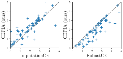
Figure 4: Scatter plots of the costs on the GMC dataset.

Figure 4 shows scatter plots of the cost for each instance, where the x-axis (resp. y-axis) stands for the cost of the baselines (resp. CEPIA). The valid ratios of ImputationCE, RobustCE, and CEPIA are 47.3%, 100%, and 100%, respectively. Similar to the results on the MCAR, we can see that the valid ratio of ImputationCE was significantly lower than RobustCE and CEPIA, and the costs of RobustCE were always larger than CEPIA. These results indicate that our CEPIA could yield better actions than the baselines under the MAR situation as well.

In Table 2c of Section 1, we examine imputation-action pairs extracted by CEPIA. Table 2c shows that CEPIA extracted various imputation candidates. Moreover, their actions differ in the validity, cost, and features to be changed, though only the feature “MonthlyIncome" was missing. It suggests that our CEPIA succeeded in yielding a representative set of imputation-action pairs, which includes valid actions and clarifies how imputation affects the resulting actions.

4.2.3 Demonstration with Real Missing Values

Table 3: An example of imputation-action pairs obtained by CEPIA on the PID dataset. For the instance, the features “SkinThickness" and “Insulin" are missing.

		Features	Values (Ranges)
Pair 1	Imputation	SkinThickness	50.3 (32.9, 53.6)
		Insulin	304.0 (14.0, 373.1)
	Action	Glucose	$-68.8$
		BMI	$-0.34$
Pair 2	Imputation	SkinThickness	36.8 (22.0, 39.3)
		Insulin	129.9 (14.0, 378.0)
	Action	Glucose	$-56.0$
Pair 3	Imputation	SkinThickness	21.3 (7.0, 28.9)
		Insulin	311.7 (14.0, 472.2)
	Action	Glucose	$-48.4$
		BloodPressure	$+0.07$
		BMI	$-0.34$

Finally, we examined our CEPIA with real missing values. We used the Pima Indians Diabetes (PID) dataset ($D=8$) (Dua and Graff, 2017). We trained the LR classifier with instances that have no missing value, and extracted actions for instances including missing values by CEPIA.

Table 3 presents an example for an instance where the features “SkinThickness" and “Insulin" are missing. In Table 3, “Ranges" indicates the estimated value range of each feature where the action is valid with the lowest cost among the obtained actions. Unfortunately, since the true value of the missing features are unknown, we cannot discuss which imputation-action pair is appropriate by simply comparing the pairs. However, focusing on “Ranges," we see that the overlapped range of “SkinThickness" among the pairs is less than “Insulin," which suggests that “SkinThickness" has more influence on the resulting action. Such a suggestion is valuable in practice to decide which missing feature should be measured next (Saar-Tsechansky and Provost, 2007).

5 Conclusion

In this paper, we first tackled the problem of CE with missing values. We empirically and theoretically showed the risk that actions are affected by imputation of missing values. To obtain valid actions with low costs for instances with missing values and clarify how imputation affects actions, we proposed Counterfactual Explanation by Pairs of Imputation and Action (CEPIA) that provides a set of pairs of an imputation candidate and its optimal action. We formulated the task of finding such a set as a submodular maximization problem. Our numerical experiments showed the efficacy of CEPIA in comparison with existing CE methods.

Limitations and future work.

There are several future directions to make our CEPIA more practical. Firstly, since the computational time of CEPIA mainly depends on calculating $a^{\ast}(\hat{x})$, developing an algorithm for Problem 1 without such computation is important. Secondly, our CEPIA implicitly assumes the MCAR mechanism since it samples each missing feature independently. To improve the efficiency, we are interested in extending our imputation sampling to the MAR or MNAR mechanism by combining recent techniques of imputation (Murray, 2018; Zhao and Udell, 2020; Ma and Zhang, 2021). Finally, extending our framework to other explanation methods, such as LIME (Ribeiro et al., 2016), is also an interesting future work.

Appendix A Omitted Proofs

A.1 Proof of Theorem 1

To prove Theorem 1, we use the following lemma by [Ustun et al., 2019, Pawelczyk et al., 2022a]. Recall that we are given (i) a classifier $h_{\beta}(x)=\operatorname{sgn}(f_{\beta}(x))$ with a linear decision function $f_{\beta}(x)=\beta^{\top}x$ and a parameter $\beta\in\mathbb{R}^{D}$, (ii) a feasible action set $\mathcal{A}(x)=\mathbb{R}^{D}$ for any $x\in\mathcal{X}$, and (iii) a cost function $c(a\mid x)=c_{x}\cdot\|a\|$, where $c_{x}>0$ is a constant depending on $x$.

Lemma 1 (Closed-form Optimal Action [Ustun et al., 2019, Pawelczyk et al., 2022a]).

For a given instance $x\in\mathcal{X}$ without missing values, let $a^{\ast}(x)$ be an optimal solution to the problem (2) for $x$. Then, we have

$$a^{\ast}(x)=\begin{cases}-\frac{f_{\beta}(x)}{\|\beta\|_{2}^{2}}\beta&\text{if }h_{\beta}(x)=-1,\\ \bm{0}&\text{otherwise}.\end{cases}$$ (5)

Using Lemma 1, we give a prove of Theorem 1 as follows. As mentioned in the main paper, we assume that a feature $d^{\circ}\in[D]$ is missing and imputed with its population mean $\mu_{d^{\circ}}=\mathbb{E}_{x}\left[x_{d^{\circ}}\right]$.

Proof of Theorem 1.

Recall that $\hat{x}_{d^{\circ}}=\mu_{d^{\circ}}$ and $\hat{x}_{d}=x_{d}$ for $d\in[D]\setminus\{d^{\circ}\}$. From Lemma 1, we obtain

$$\|a^{\ast}(\hat{x})-a^{\ast}(x)\|_{2}^{2}=\begin{cases}\frac{\beta_{d^{\circ}}^{2}}{\|\beta\|_{2}^{2}}\cdot(x_{d^{\circ}}-\mu_{d^{\circ}})^{2}&\text{if }h_{\beta}(x)=-1\land h_{\beta}(\hat{x})=-1,\\ \frac{1}{\|\beta\|_{2}^{2}}\cdot(f_{\beta}(x))^{2}&\text{if }h_{\beta}(x)=-1\land h_{\beta}(\hat{x})=+1,\\ \frac{1}{\|\beta\|_{2}^{2}}\cdot(f_{\beta}(\hat{x}))^{2}&\text{if }h_{\beta}(x)=+1\land h_{\beta}(\hat{x})=-1,\\ \bm{0}&\text{otherwise}.\end{cases}$$

Thus, we have

$$\mathbb{E}_{x}\left[\|a^{\ast}(\hat{x})-a^{\ast}(x)\|_{2}^{2}\right]= \frac{\beta_{d^{\circ}}^{2}}{\|\beta\|_{2}^{2}}\cdot\mathbb{E}_{x}\left[(x_{d^{\circ}}-\mu_{d^{\circ}})^{2}\mid h_{\beta}(x)=-1\land h_{\beta}(\hat{x})=-1\right]\cdot\mathbb{P}_{x}\left[h_{\beta}(x)=-1\land h_{\beta}(\hat{x})=-1\right]$$

$$+\frac{1}{\|\beta\|_{2}^{2}}\cdot\mathbb{E}_{x}\left[\left(f_{\beta}(x)\right)^{2}\mid h_{\beta}(x)=-1\land h_{\beta}(\hat{x})=+1\right]\cdot\mathbb{P}_{x}\left[h_{\beta}(x)=-1\land h_{\beta}(\hat{x})=+1\right]$$

$$+\frac{1}{\|\beta\|_{2}^{2}}\cdot\mathbb{E}_{x}\left[\left(f_{\beta}(\hat{x})\right)^{2}\mid h_{\beta}(x)=+1\land h_{\beta}(\hat{x})=-1\right]\cdot\mathbb{P}_{x}\left[h_{\beta}(x)=+1\land h_{\beta}(\hat{x})=-1\right].$$

For the case of $h_{\beta}(x)=+1\land h_{\beta}(\hat{x})=-1$, we have

$$(f_{\beta}(\hat{x}))^{2} =\left(f_{\beta}({x})-\beta_{d^{\circ}}(x_{d^{\circ}}-\mu_{d^{\circ}})\right)^{2}$$

$$=\left(f_{\beta}(x)\right)^{2}+\beta_{d^{\circ}}^{2}(x_{d^{\circ}}-\mu_{d^{\circ}})^{2}-2\cdot f_{\beta}(x)\cdot\beta_{d^{\circ}}(x_{d^{\circ}}-\mu_{d^{\circ}}).$$

Since $h_{\beta}(x)=+1$ and $h_{\beta}(\hat{x})=-1$, $f_{\beta}(x)\leq 0$ and $f_{\beta}(x)\leq f_{\beta}(\hat{x})\iff\beta_{d^{\circ}}(x_{d^{\circ}}-\mu_{d^{\circ}})\leq 0$ hold. Thus, we obtain

$$\left(f_{\beta}(\hat{x})\right)^{2}\leq\left(f_{\beta}(x)\right)^{2}+\beta_{d^{\circ}}^{2}(x_{d^{\circ}}-\mu_{d^{\circ}})^{2}.$$

By combining the above results, we have

$$\mathbb{E}_{x}\left[\|a^{\ast}(\hat{x})-a^{\ast}(x)\|_{2}^{2}\right]\leq \frac{\beta_{d^{\circ}}^{2}}{\|\beta\|_{2}^{2}}\cdot\mathbb{E}_{x}\left[(x_{d^{\circ}}-\mu_{d^{\circ}})^{2}\mid h_{\beta}(x)=-1\right]\cdot\mathbb{P}_{x}\left[h_{\beta}(x)=-1\right]$$

$$+\frac{1}{\|\beta\|_{2}^{2}}\cdot\mathbb{E}_{x}\left[\left(f_{\beta}(x)\right)^{2}\mid h_{\beta}(x)\not=h_{\beta}(\hat{x})\right]\cdot\mathbb{P}_{x}\left[h_{\beta}(x)\not=h_{\beta}(\hat{x})\right]$$

$$\leq \frac{\beta_{d^{\circ}}^{2}}{\|\beta\|_{2}^{2}}\cdot\mathbb{E}_{x}\left[(x_{d^{\circ}}-\mu_{d^{\circ}})^{2}\right]+\frac{1}{\|\beta\|_{2}^{2}}\cdot\gamma\cdot p_{\mathrm{conf}},$$

where $\gamma=\mathbb{E}_{x}[\left(f_{\beta}(x)\right)^{2}\mid h_{\beta}(x)\not=h_{\beta}(\hat{x})]$ and $p_{\mathrm{conf}}=\mathbb{P}_{x}[h_{\beta}(x)\not=h_{\beta}(\hat{x})]$. The final inequality holds because $(x_{d^{\circ}}-\mu_{d^{\circ}})^{2}\geq 0$ and

$$\mathbb{E}_{x}\left[(x_{d^{\circ}}-\mu_{d^{\circ}})^{2}\right]= \mathbb{E}_{x}\left[(x_{d^{\circ}}-\mu_{d^{\circ}})^{2}\mid h_{\beta}(x)=-1\right]\cdot\mathbb{P}_{x}\left[h_{\beta}(x)=-1\right]$$

$$+\mathbb{E}_{x}\left[(x_{d^{\circ}}-\mu_{d^{\circ}})^{2}\mid h_{\beta}(x)=+1\right]\cdot\mathbb{P}_{x}\left[h_{\beta}(x)=+1\right]$$

$$\geq \mathbb{E}_{x}\left[(x_{d^{\circ}}-\mu_{d^{\circ}})^{2}\mid h_{\beta}(x)=-1\right]\cdot\mathbb{P}_{x}\left[h_{\beta}(x)=-1\right].$$

Since $\sigma^{2}_{d^{\circ}}=\mathbb{E}_{x}\left[(x_{d^{\circ}}-\mu_{d^{\circ}})^{2}\right]$, we obtain

$$\mathbb{E}_{x}\left[\|a^{\ast}(\hat{x})-a^{\ast}(x)\|_{2}^{2}\right]\leq\frac{1}{\|\beta\|_{2}^{2}}\left(\beta_{d^{\circ}}^{2}\cdot\sigma_{d^{\circ}}^{2}+\gamma\cdot p_{\mathrm{conf}}\right).$$

∎

By a similar argument, we obtain an upper bound on the expected difference $\mathbb{E}_{x}\left[\|a^{\ast}(\hat{x})-a^{\ast}(x)\|_{2}^{2}\right]$ for a more general imputation method in the following theorem. Theorem 1 can be regarded as a special case of the following.

Theorem 5.

Let $i_{d^{\circ}}\colon\tilde{\mathcal{X}}\to\mathcal{X}_{d^{\circ}}$ be an imputation function for the feature $d^{\circ}$. For an instance $x\in\mathcal{X}$, we denote its incomplete instance $\tilde{x}\in\tilde{\mathcal{X}}$ (resp. its imputed instance $\hat{x}\in\mathcal{X}$) with $\tilde{x}_{d^{\circ}}=*$ (resp. $\hat{x}_{d^{\circ}}=i_{d^{\circ}}(\tilde{x})$) and $\tilde{x}_{d}=x_{d}$ (resp. $\hat{x}_{d}=x_{d}$) for $d\in[D]\setminus\{d^{\circ}\}$. Then, we have

$$\mathbb{E}_{x}\left[\|a^{\ast}(\hat{x})-a^{\ast}(x)\|_{2}^{2}\right]\leq\frac{1}{\|\beta\|_{2}^{2}}\left(\beta_{d^{\circ}}^{2}\cdot\gamma_{\mathrm{loss}}+\gamma\cdot p_{\mathrm{conf}}\right),$$ (6)

where $\gamma_{\mathrm{loss}}=\mathbb{E}_{x}\left[(x_{d^{\circ}}-i_{d^{\circ}}(\tilde{x}))^{2}\right]$ is the expected squared loss of the imputation function $i_{d^{\circ}}$. Furthermore, if $i_{d^{\circ}}$ satisfies $\mathbb{E}_{x}\left[i_{d^{\circ}}(\tilde{x})\right]=\mu_{d^{\circ}}$, then we have

$$\mathbb{E}_{x}\left[\|a^{\ast}(\hat{x})-a^{\ast}(x)\|_{2}^{2}\right]\leq\frac{1}{\|\beta\|_{2}^{2}}\left(\beta_{d^{\circ}}^{2}\cdot(\sigma_{d^{\circ}}^{2}+\gamma_{\mathrm{cov}})+\gamma\cdot p_{\mathrm{conf}}\right),$$ (7)

where $\gamma_{\mathrm{cov}}=\sigma_{\mathrm{imp}}^{2}-2\cdot\operatorname{Cov}(x_{d^{\circ}},i_{d^{\circ}}(\tilde{x}))$, $\sigma_{\mathrm{imp}}^{2}=\mathbb{E}_{x}\left[(i_{d^{\circ}}(\tilde{x})-\mu_{d^{\circ}})^{2}\right]$ is the variance of $i_{d^{\circ}}(\tilde{x})$ on $\mathcal{D}_{X}$, and $\operatorname{Cov}(x_{d^{\circ}},i_{d^{\circ}}(\tilde{x}))=\mathbb{E}_{x}\left[(x_{d^{\circ}}-\mu_{d^{\circ}})(i_{d^{\circ}}(\tilde{x})-\mu_{d^{\circ}})\right]$ is the covariance between $x_{d^{\circ}}$ and $i_{d^{\circ}}(\tilde{x})$ on $\mathcal{D}_{X}$.

Proof.

As with the proof of Theorem 4, we obtain

$$\mathbb{E}_{x}\left[\|a^{\ast}(\hat{x})-a^{\ast}(x)\|_{2}^{2}\right] \leq\frac{1}{\|\beta\|_{2}^{2}}\left(\beta_{d^{\circ}}^{2}\cdot\mathbb{E}_{x}\left[(x_{d^{\circ}}-i_{d^{\circ}}(\tilde{x}))^{2}\right]+\gamma\cdot p_{\mathrm{conf}}\right)$$

$$=\frac{1}{\|\beta\|_{2}^{2}}\left(\beta_{d^{\circ}}^{2}\cdot\gamma_{\mathrm{loss}}+\gamma\cdot p_{\mathrm{conf}}\right).$$

For the term $\gamma_{\mathrm{loss}}$, if $\mathbb{E}_{x}\left[i_{d^{\circ}}(\tilde{x})\right]=\mu_{d^{\circ}}$ holds, we also obtain

$$\gamma_{\mathrm{loss}} =\mathbb{E}_{x}\left[(x_{d^{\circ}}-i_{d^{\circ}}(\tilde{x}))^{2}\right]$$

$$=\mathbb{E}_{x}\left[(x_{d^{\circ}}-i_{d^{\circ}}(\tilde{x})-\mu_{d^{\circ}}+\mu_{d^{\circ}})^{2}\right]$$

$$=\mathbb{E}_{x}\left[(x_{d^{\circ}}-\mu_{d^{\circ}})^{2}\right]+\mathbb{E}_{x}\left[(i_{d^{\circ}}(\tilde{x})-\mu_{d^{\circ}})^{2}\right]-2\mathbb{E}_{x}\left[(x_{d^{\circ}}-\mu_{d^{\circ}})(i_{d^{\circ}}(\tilde{x})-\mu_{d^{\circ}})\right]$$

$$=\sigma_{d^{\circ}}^{2}+\sigma_{\mathrm{imp}}^{2}-2\cdot\operatorname{Cov}(x_{d^{\circ}},i_{d^{\circ}}(\tilde{x}))=\sigma_{d^{\circ}}^{2}+\gamma_{\mathrm{cov}},$$

which concludes the proof. ∎

A.2 Proof of Theorem 2

Proof of Theorem 2.

We consider to bound the probability that $\|\hat{x}-x\|_{\infty}>\varepsilon$ holds for any $\hat{x}\in\hat{\mathcal{I}}(\tilde{x})$ by $\delta$. Recall that $\hat{\mathcal{I}}(\tilde{x})$ is a set of $N$ i.i.d. imputation candidates sampled over the uniform distribution $\mathcal{D}_{I}$ on the imputation space $\mathcal{I}(\tilde{x})$. Since $\|\hat{x}-x\|_{\infty}>\varepsilon\iff\exists d\in M(\tilde{x}):|\hat{x}_{d}-x_{d}|>\varepsilon$ holds and $\mathbb{P}\left[|\hat{x}_{d}-x_{d}|\leq\varepsilon\right]=\frac{2\cdot\varepsilon}{w}$ for all $d\in[D]$, we have

$$\mathbb{P}\left[\bigcap_{\hat{x}\in\hat{\mathcal{I}}(\tilde{x})}(\|\hat{x}-x\|_{\infty}>\varepsilon)\right] =\mathbb{P}\left[\bigcap_{\hat{x}\in\hat{\mathcal{I}}(\tilde{x})}\left(\bigcup_{d\in M(\tilde{x})}(|\hat{x}_{d}-x_{d}|>\varepsilon)\right)\right]$$

$$=\left(\mathbb{P}\left[\bigcup_{d\in M(\tilde{x})}(|\hat{x}_{d}-x_{d}|>\varepsilon)\right]\right)^{N}$$

$$=\left(1-\prod_{d\in M(\tilde{x})}\mathbb{P}\left[|\hat{x}_{d}-x_{d}|\leq\varepsilon\right]\right)^{N}$$

$$=\left(1-\left(\frac{2\cdot\varepsilon}{w}\right)^{\tilde{D}}\right)^{N}\leq\exp\left(-N\cdot\left(\frac{2\cdot\varepsilon}{w}\right)^{\tilde{D}}\right),$$

where $\tilde{D}=|M(\tilde{x})|$. Therefore, we obtain

$$\exp\left(-N\cdot\left(\frac{2\cdot\varepsilon}{w}\right)^{\tilde{D}}\right)\leq\delta\iff N\geq\log\frac{1}{\delta}\cdot\left(\frac{w}{2\cdot\varepsilon}\right)^{\tilde{D}}.$$

∎

A.3 Proof of Theorem 3

Proof of Theorem 3.

To show that our objective function $g$ is non-negative, monotone, and submodular, we first decompose $g$ as $g(\mathcal{S})=\frac{1}{N}\sum_{n=1}^{N}g_{n}(\mathcal{S})$, where

$$g_{n}(\mathcal{S})\coloneqq C-l(\hat{x}^{(n)};\mathcal{S}).$$

In the following, we show that $g_{n}$ is non-negative, monotone, and submodular.

Firstly, we show that $g_{n}$ is non-negative and monotone. Let $\mathcal{S}_{1},\mathcal{S}_{2}\subset\hat{\mathcal{V}}(\tilde{x})$ be two sets of imputation-action pairs such that $\mathcal{S}_{1}\subset\mathcal{S}_{2}$. Recall that our loss function $l$ is defined as $l(x;\mathcal{S})=\min_{\hat{a}\in\mathcal{S}(x)}c(\hat{a}\mid x)$ if $|\mathcal{S}(x)|>0$ and $l(x;\mathcal{S})=0$ otherwise, where $\mathcal{S}(x)=\{\hat{a}\in\mathcal{A}(x)\mid(\hat{x},\hat{a})\in\mathcal{S}\land h(x+\hat{a})=+1\}$. Then, because $\mathcal{S}_{1}(x^{(n)})\subset\mathcal{S}_{2}(x^{(n)})$ holds for any $n\in[N]$, $l(\hat{x}^{(n)};\mathcal{S}_{1})\geq l(\hat{x}^{(n)};\mathcal{S}_{2})$ holds from the definitions of $l$. Thus, we have $g_{n}(\mathcal{S}_{1})\leq g_{n}(\mathcal{S}_{2})$, which implies the monotonicity of $g_{n}$. Furthermore, $g_{n}(\emptyset)=0$ holds because $l(\hat{x}^{(n)};\emptyset)=C$. From these results, $g_{n}$ is non-negative and monotone.

Next, to show that $g_{n}$ is submodular, we prove that the following inequality holds for any $\mathcal{S}\subseteq\hat{\mathcal{V}}(\tilde{x})$ and $p_{1},p_{2}\in\hat{\mathcal{V}}(\tilde{x})\setminus\mathcal{S}$:

$$g_{n}(\mathcal{S}\cup\{p_{1}\})+g_{n}(\mathcal{S}\cup\{p_{2}\})\geq g_{n}(\mathcal{S}\cup\{p_{1},p_{2}\})+g_{n}(\mathcal{S}).$$ (8)

Without loss of generality, we assume $l(\hat{x}^{(n)};\mathcal{S}\cup\{p_{1}\})\geq l(\hat{x}^{(n)};\mathcal{S}\cup\{p_{2}\})$. Then, $l(\hat{x}^{(n)};\mathcal{S}\cup\{p_{1},p_{2}\})=l(\hat{x}^{(n)};\mathcal{S}\cup\{p_{2}\})$ holds from the definitions of $l$, and thus we have $g_{n}(\mathcal{S}\cup\{p_{1},p_{2}\})=g_{n}(\mathcal{S}\cup\{p_{2}\})$. We also have $g_{n}(\mathcal{S}\cup\{p_{1}\})\geq g_{n}(\mathcal{S})$ from the monotonicity of $g_{n}$. By combining these results, Equation 8 holds, and thus $g_{n}$ is submodular.

From the above results, $g_{n}$ is non-negative, monotone, and submodular. Since $g$ is a convex combination of $g_{n}$, $g$ also becomes non-negative, monotone, and submodular. ∎

A.4 Proof of Theorem 4

To prove Theorem 4, we first show a property of approximate solutions to Problem 1. The following lemma shows an approximation property of an $\alpha$-approximation solution $\mathcal{S}_{\alpha}$ in the sense of the empirical average $\hat{L}$ of our loss function $l$ in the problem (4).

Lemma 2.

For $\alpha\in[0,1]$, let $\mathcal{S}_{\alpha}\subset\hat{\mathcal{V}}(\tilde{x})$ be an $\alpha$-approximation solution to Problem 1 such that $|\mathcal{S}_{\alpha}|\leq k$ and $g(\mathcal{S}_{\alpha})\geq\alpha\cdot\max_{\mathcal{S}\subset\hat{\mathcal{V}}(\tilde{x}):|\mathcal{S}|\leq k}g(\mathcal{S})$ hold. Then, $\hat{L}(\mathcal{S}_{\alpha})\leq\alpha\cdot\hat{L}(\mathcal{S})+C\cdot(1-\alpha)$ holds for any $\mathcal{S}\subset\hat{\mathcal{V}}(\tilde{x})$ such that $|\mathcal{S}|\leq k$.

Proof.

From the definition of $\alpha$-approximation solutions, $g(\mathcal{S}_{\alpha})\geq\alpha\cdot g(\mathcal{S})$ holds for any $\mathcal{S}\subset\hat{\mathcal{V}}(\tilde{x})$ such that $|\mathcal{S}|\leq k$. Therefore, we obtain

$$g(\mathcal{S}_{\alpha})\geq\alpha\cdot g(\mathcal{S}) \iff C-\hat{L}(\mathcal{S}_{\alpha})\geq\alpha\cdot(C-\hat{L}(\mathcal{S}))$$

$$\iff\hat{L}(\mathcal{S}_{\alpha})\leq\alpha\cdot\hat{L}(\mathcal{S})+C\cdot(1-\alpha).$$

∎

Next, we show an approximation guarantee of the empirical loss $\hat{L}$ for the expected loss $L$ in the following lemma.

Lemma 3.

For any $\delta>0$, the following inequality holds for any $\mathcal{S}\subset\hat{\mathcal{V}}(\tilde{x})$ such that $|\mathcal{S}|\leq k$ with probability $1-\delta$:

$$|L(\mathcal{S})-\hat{L}(\mathcal{S})|\leq C\cdot\sqrt{\frac{k\cdot\ln N+\ln\frac{2}{\delta}}{2\cdot N}}.$$ (9)

Proof.

Firstly, we consider the probability of $|L(\mathcal{S})-\hat{L}(\mathcal{S})|>\varepsilon$ for some $\varepsilon>0$ and a fixed $\mathcal{S}\subset\hat{\mathcal{V}}(\tilde{x})$. Recall that our loss $l(x;\mathcal{S})$ is bounded in $[0,C]$ from the definition, and that $L(\mathcal{S})$ and $\hat{L}(\mathcal{S})$ are the expected value of our loss $l$ over the distribution $\mathcal{D}_{I}$ and the empirical average of $l$ over a finite set of $N$ i.i.d. samples drown from $\mathcal{D}_{I}$, respectively. Hence, by applying Hoeffding’s inequality [Mohri et al., 2012], we have

$$\mathbb{P}[|L(\mathcal{S})-\hat{L}(\mathcal{S})|>\varepsilon]\leq 2\cdot\exp\left(\frac{-2\cdot N\cdot\varepsilon^{2}}{C^{2}}\right).$$

Next, we consider to bound the probability that there exists $\mathcal{S}\subset\hat{\mathcal{V}}(\tilde{x})$ such that $|\mathcal{S}|\leq k$ and $|L(\mathcal{S})-\hat{L}(\mathcal{S})|>\varepsilon$ by $\delta$. Using the union bound, we have

$$\mathbb{P}\left[\bigcup_{\mathcal{S}\subset\hat{\mathcal{V}}(\tilde{x}):|\mathcal{S}|\leq k}\left(|L(\mathcal{S})-\hat{L}(\mathcal{S})|>\varepsilon\right)\right] \leq\sum_{\mathcal{S}\subset\hat{\mathcal{V}}(\tilde{x}):|\mathcal{S}|\leq k}\mathbb{P}\left[|L(\mathcal{S})-\hat{L}(\mathcal{S})|>\varepsilon\right]$$

$$\leq N^{k}\cdot 2\cdot\exp\left(\frac{-2\cdot N\cdot\varepsilon^{2}}{C^{2}}\right).$$

Therefore, we obtain

$$N^{k}\cdot 2\cdot\exp\left(\frac{-2\cdot N\cdot\varepsilon^{2}}{C^{2}}\right)=\delta\iff\varepsilon=C\cdot\sqrt{\frac{k\cdot\ln N+\ln\frac{2}{\delta}}{2\cdot N}},$$

which concludes the proof. ∎

Using Lemmas 2 and 3, we can proof Theorem 4 as follows.

Proof of Theorem 1.

For $\tilde{x}\in\tilde{\mathcal{X}}$, let $\hat{\mathcal{S}}\subset\hat{\mathcal{V}}(\tilde{x})$ be a set of imputation-action pairs that minimizes $L(\mathcal{S})$ over $\hat{\mathcal{V}}(\tilde{x})$ under the constraint $|\mathcal{S}|\leq k$; that is, $\hat{\mathcal{S}}\coloneqq\arg\min_{\mathcal{S}\subset\hat{\mathcal{V}}(\tilde{x}):|\mathcal{S}|\leq k}L(\mathcal{S})$. From Lemma 2, we have

$$L(\mathcal{S}_{\alpha})-L(\mathcal{S}^{*}) =L(\mathcal{S}_{\alpha})-\hat{L}(\mathcal{S}_{\alpha})+\hat{L}(\mathcal{S}_{\alpha})-L(\hat{\mathcal{S}})+L(\hat{\mathcal{S}})-L(\mathcal{S}^{*})$$

$$\leq L(\mathcal{S}_{\alpha})-\hat{L}(\mathcal{S}_{\alpha})+\alpha\cdot\hat{L}(\hat{\mathcal{S}})-L(\hat{\mathcal{S}})+\gamma_{\mathrm{bias}}+\gamma_{\mathrm{approx}},$$

where $\gamma_{\mathrm{bias}}=L(\hat{\mathcal{S}})-L(\mathcal{S}^{*})$ and $\gamma_{\mathrm{approx}}=C\cdot(1-\alpha)$. Since $\mathcal{S}_{\alpha},\hat{\mathcal{S}}\subset\hat{\mathcal{V}}(\tilde{x})$, $|\mathcal{S}_{\alpha}|\leq k$, $|\hat{\mathcal{S}}|\leq k$, and $\alpha\cdot\hat{L}(\hat{\mathcal{S}})\leq\hat{L}(\hat{\mathcal{S}})$, we have

$$L(\mathcal{S}_{\alpha})-\hat{L}(\mathcal{S}_{\alpha})+\alpha\cdot\hat{L}(\hat{\mathcal{S}})-L(\hat{\mathcal{S}}) \leq L(\mathcal{S}_{\alpha})-\hat{L}(\mathcal{S}_{\alpha})+\hat{L}(\hat{\mathcal{S}})-L(\hat{\mathcal{S}})$$

$$\leq 2\cdot\max_{\mathcal{S}\subset\hat{\mathcal{V}}(\tilde{x}):|\mathcal{S}|\leq k}|L(\mathcal{S})-\hat{L}(\mathcal{S})|.$$

From Lemma 3, the following inequality holds with probability $1-\delta$ for any $\delta>0$:

$$2\cdot\max_{\mathcal{S}\subset\hat{\mathcal{V}}(\tilde{x}):|\mathcal{S}|\leq k}|L(\mathcal{S})-\hat{L}(\mathcal{S})| \leq 2\cdot\sqrt{\frac{k\cdot\ln N+\ln\frac{2}{\delta}}{2\cdot N}}=\gamma_{\mathrm{var}},$$

where $\gamma_{\mathrm{var}}=C\cdot\sqrt{(2/N)\cdot(k\cdot\ln N+\ln(2/\delta))}$. From these results, we obtain $L(\mathcal{S}_{\alpha})-L(\mathcal{S}^{\ast})\leq\gamma_{\mathrm{bias}}+\gamma_{\mathrm{var}}+\gamma_{\mathrm{approx}}$ with probability $1-\delta$. ∎

Appendix B Counterfactual Explanation by Mixed-Integer Linear Optimization

As an oracle for solving the problem (2), we employ the existing CE methods based on mixed-integer linear optimization (MILO) [Ustun et al., 2019, Cui et al., 2015, Kanamori et al., 2020, 2021, Parmentier and Vidal, 2021]. These methods formulate the problem (2) as an MILO problem, which can be solved using off-the-shelf MILO solvers such as Gurobi or CPLEX, and then recover the optimal action from the optimal solution to the formulated MILO problem. In this section, we review the existing MILO formulations of the problem (2) for linear classifiers, deep ReLU networks, and tree ensembles.

B.1 Common Ideas

As with the existing methods based on MILO [Ustun et al., 2019, Kanamori et al., 2020], we assume that each coordinate $A_{d}$ of a given feasible action set $\mathcal{A}(x)=A_{1}\times\dots\times A_{D}$ is finite and discretized; that is, we assume $A_{d}=\{a_{d,1},\dots,a_{d,J_{d}}\}$, where $J_{d}=|A_{d}|$. For simplicity, we also assume that the cost function $c$ can be expressed as the following linear form:

$$c(a\mid x)=\sum_{d=1}^{D}c_{d}(a_{d}\mid x_{d}),$$

where $c_{d}\colon A_{d}\to\mathbb{R}_{\geq 0}$ is a cost measure of the feature $d$ that represents the effort to change $x_{d}$ to $x_{d}+a_{d}$. It includes several existing cost functions, such as the TLPS [Ustun et al., 2019] and MAD [Wachter et al., 2018]. Note that the formulations described below can be extended to handle existing non-linear cost functions, such as the max percentile shift [Ustun et al., 2019] and local outlier factor [Kanamori et al., 2020].

To express an action $a\in\mathcal{A}(x)$, we introduce binary variables $\pi_{d,j}\in\{0,1\}$ for $d\in[D]$ and $j\in[J_{d}]$, which indicate that the action $a_{d,j}\in A_{d}$ is selected ($\pi_{d,j}=1$) or not ($\pi_{d,j}=0$). The variables $\pi_{d,j}$ must satisfy the following constraint for $d\in[D]$:

$$\sum_{j=1}^{J_{d}}\pi_{d,j}=1.$$

Using $\pi_{d,j}$, each element $a_{d}$ of $a=(a_{1},\dots,a_{D})$ can be expressed as $a_{d}=\sum_{j=1}^{J_{d}}a_{d,j}\cdot\pi_{d,j}$, and the objective function $c(a\mid x)$ of the problem (2) can be expressed as follows:

$$c(a\mid x)=\sum_{d=1}^{D}\sum_{j=1}^{J_{d}}c_{d}(a_{d,j}\mid x_{d})\cdot\pi_{d,j}.$$

Note that $c_{d}(a_{d,j}\mid x_{d})$ is a constant because it can be computed when $x$ and $\mathcal{A}(x)$ are given.

To formulate the problem (2) as an MILO problem, we need to express the constraint $h(x+a)=+1$ as linear constraints of decision variables for each type of classifiers $h$. In the following, we present an MILO formulation of the problem (2) for each classifier.

B.2 Linear Classifier

Let $h$ be a linear classifier $h(x)=\operatorname{sgn}\left(\beta^{\top}x\right)$, where $\beta=(\beta_{1},\dots,\beta_{D})\in\mathbb{R}^{D}$ is a coefficient vector. Then, the problem (2) with the linear classifier $h$ can be formulated as the following MILO problem [Ustun et al., 2019]:

$$\begin{array}[]{cl}\text{minimize}&\displaystyle\sum_{d=1}^{D}\sum_{j=1}^{J_{d}}c_{d}(a_{d,j}\mid x_{d})\cdot\pi_{d,j}\\ \text{subject to}&\displaystyle\sum_{j=1}^{J_{d}}\pi_{d,j}=1,\forall d\in[D],\\ &\displaystyle\sum_{d=1}^{D}\beta_{d}\cdot\sum_{j=1}^{J_{d}}a_{d,j}\cdot\pi_{d,j}+\beta^{\top}x\geq 0,\\ &\displaystyle\pi_{d,j}\in\{0,1\},\forall d\in[D],\forall j\in[J_{d}].\end{array}$$

B.3 Deep ReLU Networks

For simplicity, we focus on a two-layer ReLU network $h(x)=\operatorname{sgn}\left(\sum_{t=1}^{T}\theta_{t}\cdot\max\{0,\beta_{t}^{\top}x\}\right)$, where $\beta_{t}=(\beta_{t,1},\dots,\beta_{t,D})\in\mathbb{R}^{D}$ is a coefficient vector of the $t$-th neuron, $\theta_{t}\in\mathbb{R}$ is a weight value of the $t$-th neuron, and $T\in\mathbb{N}$ is the total number of neurons in the middle layer. Then, the problem (2) with the two-layer ReLU network $h$ can be formulated as the following MILO problem [Serra et al., 2018, Kanamori et al., 2021]:

$$\begin{array}[]{cl}\text{minimize}&\displaystyle\sum_{d=1}^{D}\sum_{j=1}^{J_{d}}c_{d}(a_{d,j}\mid x_{d})\cdot\pi_{d,j}\\ \text{subject to}&\displaystyle\sum_{j=1}^{J_{d}}\pi_{d,j}=1,\forall d\in[D],\\ &\displaystyle\sum_{t=1}^{T}\theta_{t}\cdot\xi_{t}\geq 0,\\ &\displaystyle\xi_{t}\leq H_{t}\cdot\nu_{t},\forall t\in[T],\\ &\displaystyle\bar{\xi}_{t}\leq-\bar{H}_{t}\cdot(1-\nu_{t}),\forall t\in[T],\\ &\displaystyle\xi_{t}-\bar{\xi}_{t}=\sum_{d=1}^{D}\beta_{t,d}\cdot\sum_{j=1}^{J_{d}}a_{d,j}\cdot\pi_{d,j}+F_{t},\forall t\in[T],\\ &\displaystyle\pi_{d,j}\in\{0,1\},\forall d\in[D],\forall j\in[J_{d}],\\ &\displaystyle\xi_{t},\bar{\xi}_{t}\geq 0,\nu_{t}\in\{0,1\},\forall t\in[T],\end{array}$$

where $H_{t}$, $\bar{H}_{t}$, and $F_{t}$ are constants such that $H_{t}\geq\max_{a\in\mathcal{A}(x)}\beta_{t}^{\top}(x+a)$, $\bar{H}_{t}\leq\min_{a\in\mathcal{A}(x)}\beta_{t}^{\top}(x+a)$, and $F_{t}=\beta_{t}^{\top}x$, respectively. These values can be computed when $h$, $x$, and $\mathcal{A}(x)$ are given. Note that our formulation can be extended to general multilayer ReLU networks [Serra et al., 2018].

B.4 Tree Ensembles

Let $h$ be a tree ensemble $h(x)=\operatorname{sgn}\left(\sum_{t=1}^{T}\theta_{t}\cdot f_{t}(x)\right)$, where $f_{t}\colon\mathcal{X}\to\mathbb{R}$ is a decision tree, $\theta_{t}\in\mathbb{R}$ is a weight value of the $t$-th decision tree $f_{t}$, and $T\in\mathbb{N}$ is the total number of decision trees. Each decision tree $f_{t}$ can be expressed as $f_{t}(x)=\sum_{l=1}^{L_{t}}\hat{y}_{t,l}\cdot\mathbb{I}\left[x\in r_{t,l}\right]$, where $L_{t}\in\mathbb{N}$ is the total number of leaves in $f_{t}$, and $\hat{y}_{t,l}\in\mathbb{R}$ and $r_{t,l}=r^{(1)}_{t,l}\times\dots\times r^{(D)}_{t,l}\subseteq\mathcal{X}$ are the predictive label and the region corresponding to a leaf $l\in[L_{t}]$, respectively. Then, the problem (2) with the tree ensemble $h$ can be formulated as the following MILO problem [Cui et al., 2015, Kanamori et al., 2020]:

$$\begin{array}[]{cl}\text{minimize}&\displaystyle\sum_{d=1}^{D}\sum_{j=1}^{J_{d}}c_{d}(a_{d,j}\mid x_{d})\cdot\pi_{d,j}\\ \text{subject to}&\displaystyle\sum_{j=1}^{J_{d}}\pi_{d,j}=1,\forall d\in[D],\\ &\displaystyle\sum_{t=1}^{T}\theta_{t}\cdot\sum_{l=1}^{L_{t}}\hat{y}_{t,l}\cdot\phi_{t,l}\geq 0,\\ &\displaystyle\sum_{l=1}^{L_{t}}\phi_{t,l}=1,\forall t\in[T],\\ &\displaystyle D\cdot\phi_{t,l}\leq\sum_{d=1}^{D}\sum_{j\in J^{(d)}_{t,l}}\pi_{d,j},\forall t\in[T],\forall l\in[L_{t}],\\ &\displaystyle\pi_{d,j}\in\{0,1\},\forall d\in[D],\forall j\in[J_{d}],\\ &\displaystyle\phi_{t,l}\in\{0,1\},\forall t\in[T],\forall l\in[L_{t}],\end{array}$$

where $J^{(d)}_{t,l}=\{j\in[J_{d}]\mid x_{d}+a_{d,j}\in r^{(d)}_{t,l}\}$, which can be computed when $h$, $x$, and $\mathcal{A}(x)$ are given.

Appendix C Algorithms for Problem 1

Algorithm 1 Greedy algorithm [Nemhauser et al., 1978] for Problem 1.

0:   instance $\tilde{x}\in\tilde{\mathcal{X}}$ with missing values, a set of $N$ imputation candidates $\hat{\mathcal{I}}(\tilde{x})=\{\hat{x}^{(1)},\dots,\hat{x}^{(N)}\}$, and a parameter $k>0$.

0:  A set $\mathcal{S}$ of imputation-action pairs.

1:  /* Generate the ground set $\hat{\mathcal{V}}(\tilde{x})$ */

2:  $\hat{\mathcal{V}}(\tilde{x})\leftarrow\{\}$;

3:  for $n=1,\dots,N$ do

4:     $\hat{a}^{(n)}\leftarrow a^{\ast}(\hat{x}^{(n)})$;

5:     $\hat{\mathcal{V}}(\tilde{x})\leftarrow\hat{\mathcal{V}}(\tilde{x})\cup\{(\hat{x}^{(n)},\hat{a}^{(n)})\}$;

6:  end for

7:  /* Optimize the objective function $g$ greedily */

8:  $\mathcal{S}\leftarrow\{\}$;

9:  while $|\mathcal{S}|<k$ do

10:     $(\hat{x}^{\ast},\hat{a}^{\ast})\leftarrow\arg\max_{(\hat{x},\hat{a})\in\hat{\mathcal{V}}(\tilde{x})}\left(g(\mathcal{S}\cup\{(\hat{x},\hat{a})\})-g(\mathcal{S})\right)$;

11:     $\mathcal{S}\leftarrow\mathcal{S}\cup\{(\hat{x}^{\ast},\hat{a}^{\ast})\}$;

12:     $\hat{\mathcal{V}}(\tilde{x})\leftarrow\hat{\mathcal{V}}(\tilde{x})\setminus\{(\hat{x}^{\ast},\hat{a}^{\ast})\}$;

13:  end while

14:  return $\mathcal{S}$;

Algorithm 2 SampleGreedy algorithm [Harshaw et al., 2022] for Problem 1.

0:   instance $\tilde{x}\in\tilde{\mathcal{X}}$ with missing values, a set of $N$ imputation candidates $\hat{\mathcal{I}}(\tilde{x})=\{\hat{x}^{(1)},\dots,\hat{x}^{(N)}\}$, and a parameter $k>0$.

0:  A set $\mathcal{S}$ of imputation-action pairs.

1:  /* Generate the subsampled ground set $\hat{\mathcal{V}}^{\prime}(\tilde{x})\subseteq\hat{\mathcal{V}}(\tilde{x})$ */

2:  $\hat{\mathcal{V}}^{\prime}(\tilde{x})\leftarrow\{\}$;

3:  for $n=1,\dots,N$ do

4:     $\delta_{n}\leftarrow$ sample a uniformly random integer over $\{0,1\}$;

5:     if $\delta_{n}=1$ then

6:        $\hat{a}^{(n)}\leftarrow a^{\ast}(\hat{x}^{(n)})$;

7:        $\hat{\mathcal{V}}^{\prime}(\tilde{x})\leftarrow\hat{\mathcal{V}}^{\prime}(\tilde{x})\cup\{(\hat{x}^{(n)},\hat{a}^{(n)})\}$;

8:     end if

9:  end for

10:  /* Optimize the objective function $g$ greedily */

11:  $\mathcal{S}\leftarrow\{\}$;

12:  while $|\mathcal{S}|<k$ do

13:     $(\hat{x}^{\ast},\hat{a}^{\ast})\leftarrow\arg\max_{(\hat{x},\hat{a})\in\hat{\mathcal{V}}^{\prime}(\tilde{x})}\left(g(\mathcal{S}\cup\{(\hat{x},\hat{a})\})-g(\mathcal{S})\right)$;

14:     $\mathcal{S}\leftarrow\mathcal{S}\cup\{(\hat{x}^{\ast},\hat{a}^{\ast})\}$;

15:     $\hat{\mathcal{V}}^{\prime}(\tilde{x})\leftarrow\hat{\mathcal{V}}^{\prime}(\tilde{x})\setminus\{(\hat{x}^{\ast},\hat{a}^{\ast})\}$;

16:  end while

17:  return $\mathcal{S}$;

For a given instance $\tilde{x}\in\tilde{\mathcal{X}}$ with missing values, our CEPIA provides a set $\mathcal{S}$ of imputation-action pairs $(\hat{x},\hat{a})$ by solving Problem 1. As shown by Theorem 3, Problem 1 is a non-negative monotone submodular maximization problem with a cardinality constraint, which is a well-known problem class that can be efficiently solved with an approximation guarantee by a simple greedy algorithm [Nemhauser et al., 1978]. Algorithm 1 presents a greedy algorithm for Problem 1. It has a $(1-\frac{1}{e})$-approximation guarantee [Nemhauser et al., 1978]; that is, a solution $\mathcal{S}_{1}$ obtained by Algorithm 1 satisfies $g(\mathcal{S}_{1})\geq(1-\frac{1}{e})\cdot g^{\ast}$, where $g^{\ast}\coloneqq\arg\max_{\mathcal{S}\subset\hat{\mathcal{V}}(\tilde{x}):|\mathcal{S}|\leq k}g(\mathcal{S})$ is the optimal value of Problem 1.

In practice, the computational time of Algorithm 1 mainly depends on line 4, where an action $\hat{a}^{(n)}$ is optimized by calculating $a^{\ast}(\hat{x}^{(n)})$ for each $n\in[N]$. Since we calculate $a^{\ast}(\hat{x}^{(n)})$ by solving an MILO problem as shown in the previous section, Algorithm 1 often becomes computationally infeasible for a large $N$ and a complex classifier $h$ (e.g., a random forest with $T>300$ decision trees). To reduce the total number of calculating $a^{\ast}(\hat{x}^{(n)})$, we employ the SampleGreedy algorithm [Harshaw et al., 2022], which is a variant of the greedy algorithm combined with subsampling of the ground set. Algorithm 2 presents the SampleGreedy algorithm for Problem 1. In Algorithm 2, we first obtain subsamples of imputation candidates from $\hat{\mathcal{I}}(\tilde{x})$ with probability $\frac{1}{2}$, and optimize actions only for the subsampled imputation candidates $\hat{x}^{(n)}$ by calculating $a^{\ast}(\hat{x}^{(n)})$ to obtain the subsampled ground set $\hat{\mathcal{V}}^{\prime}(\tilde{x})$. Then, we run the standard greedy algorithm same with Algorithm 1 over the subsampled ground set $\hat{\mathcal{V}}^{\prime}(\tilde{x})$. Note that the objective function $g$ is exactly evaluated over $\hat{\mathcal{I}}(\tilde{x})$ without subsampling. While Algorithm 2 reduces the total number of calculating $a^{\ast}(\hat{x}^{(n)})$ compared to Algorithm 1 by subsampling the ground set, it has a $\frac{1}{2}$-approximation guarantee [Harshaw et al., 2022]; that is, a solution $\mathcal{S}_{2}$ obtained by Algorithm 2 satisfies $g(\mathcal{S}_{2})\geq\frac{1}{2}\cdot g^{\ast}$. In our experiments presented later, we observed that Algorithm 2 was about twice as fast as Algorithm 1 and could provide good solutions that are comparable with Algorithm 1.

Appendix D Post-Processing of CEPIA

Given a complete instance $x$, our CEPIA can determine an adequate action $\hat{a}^{\ast}$ from a set $\mathcal{S}$ of imputation-action pairs $(\hat{x},\hat{a})$ by $\hat{a}^{\ast}=\arg\min_{\hat{a}\in\mathcal{S}(x)}c(\hat{a}\mid x)$, where $\mathcal{S}(x)=\{\hat{a}\in\mathcal{A}(x)\mid(\hat{x},\hat{a})\in\mathcal{S}\land h(x+\hat{a})=+1\}$. However, it is often difficult for users to select an adequate action from $\mathcal{S}$ by themselves. To help users identify valid actions with low costs from $\mathcal{S}$ without disclosing their missing values, we aim to provide a region $r\subseteq\mathcal{I}(\tilde{x})$ on the imputation space for each action $\hat{a}$ in $\mathcal{S}$ where $\hat{a}$ is valid with the lowest cost among the actions in $\mathcal{S}$. Such a region $r$ can be defined as $r\coloneqq\{\hat{x}\in\mathcal{I}(\tilde{x})\mid\hat{a}=\arg\min_{a\in\mathcal{S}(\hat{x})}c(a\mid\hat{x})\}$. However, exactly calculating the region $r$ for each $\hat{a}$ is generally difficult for complex classifiers $h$ whose decision region is neither convex nor continuous, such as deep neural networks or large tree ensembles.

Instead of exact methods, we propose a heuristic method that provides a region $\hat{r}$ where each action $\hat{a}$ of $\mathcal{S}$ is estimated to be valid with the lowest cost among the actions in $\mathcal{S}$. Our idea is to estimate $r$ using the set of $N$ imputation candidates $\hat{\mathcal{I}}(\tilde{x})=\{\hat{x}^{(1)},\dots,\hat{x}^{(N)}\}$, which is used for optimizing $\mathcal{S}$. Our post-processing procedure to estimate $r$ for each $a$ in $\mathcal{S}$ consists of the following steps:

1. Let $\hat{\mathcal{I}}_{\hat{a}}(\tilde{x})\coloneqq\{\hat{x}\in\hat{\mathcal{I}}(\tilde{x})\mid\hat{a}=\arg\min_{a\in\mathcal{S}(\hat{x})}c(a\mid\hat{x})\}$ be the set of imputation candidates where the action $\hat{a}$ is valid and has the lowest cost among the actions in $\mathcal{S}$.

2. Calculate the minimum rectangle $\hat{r}\subseteq\mathcal{I}(\tilde{x})$ that includes $\hat{\mathcal{I}}_{\hat{a}}(\tilde{x})$, i.e., $\hat{r}=\hat{r}_{1}\times\dots\times\hat{r}_{D}$ with

   $$\hat{r}_{d}=[{\min}_{\hat{x}\in\hat{\mathcal{I}}_{\hat{a}}(\tilde{x})}\hat{x}_{d},{\max}_{\hat{x}\in\hat{\mathcal{I}}_{\hat{a}}(\tilde{x})}\hat{x}_{d}]$$

   for $d\in[D]$.

3. Return $\hat{r}$ as an estimated region for the action $\hat{a}$.

As shown in Theorem 2, $\hat{\mathcal{I}}(\tilde{x})$ includes at least one imputation candidate $\hat{x}$ near to a given original instance $x$ with high probability if we take a sufficiently large $N$. It suggests that we are expected to obtain a region $\hat{r}$ that includes $x$ by calculating it from $\hat{\mathcal{I}}(\tilde{x})$ for each action $\hat{a}$ in $\mathcal{S}$.

Appendix E Implementation Details of Baseline Methods

E.1 ImputationCE

As a baseline that works with missing values, we implemented a naive method that combines the existing CE methods with an imputation method. Let $i\colon\tilde{\mathcal{X}}\to\mathcal{X}$ be an imputation method that replaces the missing values of a given incomplete instance $\tilde{x}\in\tilde{\mathcal{X}}$ with some plausible values and returns an imputed instance $\hat{x}\in\mathcal{X}$. Our ImputationCE with an imputation method $i$ consists of the following two steps:

1. For a given instance $\tilde{x}\in\tilde{\mathcal{X}}$ with missing values, we obtain its imputed instance $\hat{x}=i(\tilde{x})$ by applying the imputation method $i$.

2. We optimize an action for the imputed instance $\hat{x}$ instead of $\tilde{x}$ by calculating $a^{\ast}(\hat{x})$.

As an imputation method $i$, we employ three major methods: mean imputation [Little and Rubin, 2019], $k$-NN imputation [Troyanskaya et al., 2001], and MICE [van Buuren and Groothuis-Oudshoorn, 2011]. We implemented each method using scikit-learn with its default parameters. Note that we implemented MICE with IterativeImputer that adapts MICE to be able to impute test instances, as with previous studies [Le Morvan et al., 2021].

E.2 RobustCE

As another baseline method, we extend the existing robust CE methods [Dominguez-Olmedo et al., 2022, Dutta et al., 2022, Pawelczyk et al., 2022b] to our setting. Most existing studies on robust CE aim to optimize an action that is valid even if a given instance is slightly perturbed. For a given instance $x\in\mathcal{X}$ without missing values, their task can be formulated as the following optimization problem:

$$\begin{array}[]{cll}\displaystyle\mathop{\text{minimize}}_{a\in\mathcal{A}(x)}&c(a\mid x)&\\ \text{subject to}&h(x^{\prime}+a)=+1,&\forall x^{\prime}\in B_{\varepsilon}(x),\end{array}$$

where $B_{\varepsilon}(x)=\{x^{\prime}\in\mathcal{X}\mid\|x-x^{\prime}\|\leq\varepsilon\}$ is the $\varepsilon$-ball of $x$, i.e., set of perturbed instances around $x$, for some $\varepsilon>0$. This formulation is motivated by the observation that actions $a$ are often affected by small perturbations to inputs $x$, which is similar to our observation that actions are affected by imputation.

To extend the existing robust CE methods to handle our setting with missing values, we take the following two steps: (1) obtain the imputed instance $\hat{x}=i(\tilde{x})$ by applying an imputation method $i$ (e.g., MICE [van Buuren and Groothuis-Oudshoorn, 2011]) for $\tilde{x}$, and (2) replace $B_{\varepsilon}(x)$ with a set $\hat{\mathcal{I}}(\tilde{x})\subset\mathcal{I}(\tilde{x})$ of $N$ imputation candidates randomly sampled from the distribution $\mathcal{D}_{I}$. Overall, our RobustCE method optimizes an action for $\tilde{x}$ by solving the following problem:

$$\begin{array}[]{cll}\displaystyle\mathop{\text{minimize}}_{a\in\mathcal{A}(\hat{x})}&c(a\mid\hat{x})&\\ \text{subject to}&h(\hat{x}+a)=+1,&\\ &h(\hat{x}^{\prime}+a)=+1,&\forall\hat{x}^{\prime}\in\hat{\mathcal{I}}(\tilde{x}).\end{array}$$ (13)

By solving the problem (13), we can obtain an action that is valid for any $\hat{x}^{\prime}\in(\{\hat{x}\}\cup\hat{\mathcal{I}}(\tilde{x}))$, which indicates that the obtained action may be also valid for the original instance $x$.

Fortunately, the problem (13) can be solved by extending the existing MILO-based CE methods to include linear constraints that express the additional constraints $h(\hat{x}^{\prime}+a)=+1$ for $\hat{x}^{\prime}\in\hat{\mathcal{I}}(\tilde{x})$. However, such additional constraints increase the total number of constraints in the MILO problem, which makes solving the problem (13) challenging for a large $N$ and a complex classifier $h$. To address this computational issue, we modify the optimization algorithm of the existing robust CE method proposed by [Dominguez-Olmedo et al., 2022]. Our modified algorithm for the problem (13) consists of the following steps:

1. Optimize an action $\hat{a}^{\ast}=a^{\ast}(\hat{x})$ for $\hat{x}$ by the MILO-based method without any additional constraint.

2. Find $\hat{x}^{\ast}=\arg\max_{\hat{x}^{\prime}\in\hat{\mathcal{I}}(\tilde{x})}l_{\mathrm{logistic}}(f(\hat{x}^{\prime}+\hat{a}^{\ast}),+1)$, where $l_{\mathrm{logistic}}$ is the logistic loss and $f$ is the decision function of $h$ such that $h(x)=\operatorname{sgn}(f(x))$.

3. If $h(\hat{x}^{\ast}+\hat{a}^{\ast})=+1$, then return $\hat{a}^{\ast}$

4. Update an action $\hat{a}^{\ast}$ by adding the constraint $h(\hat{x}^{\ast}+a)=+1$ to the MILO formulation and solving the MILO problem, and go to Step 2.

The above algorithm avoids increasing constraints by sequentially adding the constraint one by one to the MILO formulation. Because the action $\hat{a}^{\ast}$ obtained by the algorithm satisfies $h(\hat{x}^{\prime}+\hat{a}^{\ast})=+1$ for all $\hat{x}^{\prime}\in(\{\hat{x}\}\cup\hat{\mathcal{I}}(\tilde{x}))$ and minimizes its cost, we can guarantee that $\hat{a}^{\ast}$ is an optimal solution to the problem (13). In our experiments, we observed that the above algorithm often stopped after about $10$ iterations even for $N\geq 100$, and it was faster than adding all the constraints to the MILO formulation.

Appendix F Additional Experimental Results

F.1 Complete Results of MCAR Situation

We show complete experimental results under the MCAR mechanism. Figures 5, 6 and 7 present the complete experimental results of the valid ratio, average cost, and average sign agreement score, respectively. We also show the results of the average computational time for each method in Tables 4 and 5.

F.2 Complete Results of MAR and MNAR Situations

We show complete experimental results under the MAR and MNAR mechanisms. To simulate the MNAR mechanism, we assume a situation where richer people are less inclined to reveal their income [Josse et al., 2019]. We collected test instances that were predicted as “experiencing 90 days past due delinquency or worse" and had larger incomes than the median of the feature “MonthlyIncome." Then, as with our MAR situation, we dropped their values of the feature “MonthlyIncome" and extracted actions for them by each method.

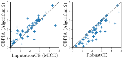
(a) MAR (TLPS)

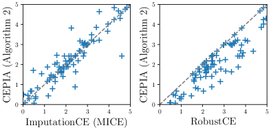
(b) MNAR (TLPS)

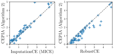
(c) MAR (MAD)

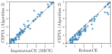
(d) MNAR (MAD)

Figure 8: Scatter plots of the costs on the GiveMeCredit dataset under the MAR and MNAR situations.

Table 6b presents the complete experimental results of the valid ratio, average cost, and average computational time. The scatter plots of the costs for ImputationCE (MICE), RobustCE, and CEPIA (Algorithm 2) are shown in Figure 8.

F.3 Sensitivity Analysis of CEPIA

To examine the sensitivity with respect to the size parameter $k$ and the sampling size $N$ of our CEPIA, we conducted sensitivity analyses of these parameters by varying these values for the LR classifier on each dataset under the MCAR mechanism.

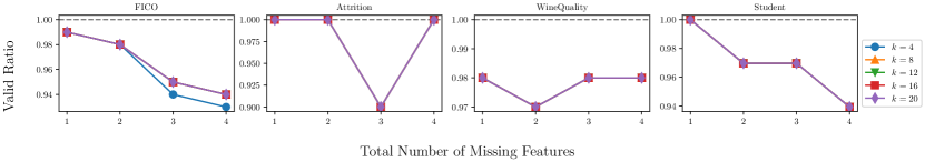
(a) Valid Ratio

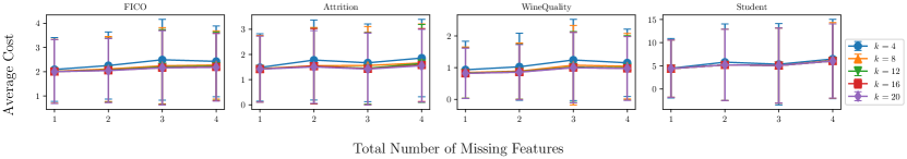
(b) Cost

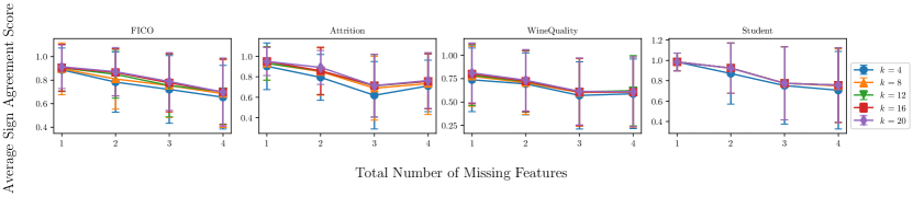
(c) Sign Agreement Score

Figure 9: Experimental results of the sensitivity analyses on the parameter $k$ for TLPS.

Firstly, the results with respect to the size parameters $k$ are shown in Figures 9 and 10. We varied the value of $k$ in $\{4,8,12,16,20\}$ with $N=100$, and measured the valid ratio, average cost, and average sign agreement score.

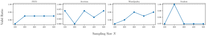
(a) Valid Ratio

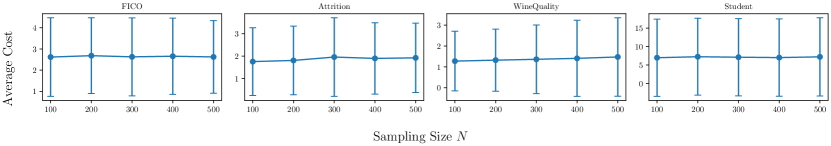
(b) Cost

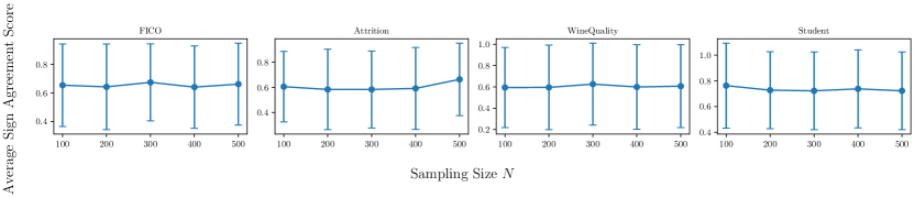
(c) Sign Agreement Score

(d) Computational Time

Figure 11: Experimental results of the sensitivity analyses on the sampling size $N$ for TLPS.

Next, the results with respect to the sampling size $N$ are shown in Figures 11 and 12. We varied the value of $N$ in $\{100,200,300,400,500\}$ with $k=4$, and measured the valid ratio, average cost, average sign agreement score, and average computational time. Note that we fixed the total number of missing features as $\tilde{D}=4$ for all the datasets.

Appendix G Additional Comments on Existing Assets

Gurobi 9.5.1 is a commercial solver for mixed-integer optimization provided by Gurobi Optimization, LLC. Scikit-learn 1.0.2 is publicly available under the BSD-3-Clause license.

All datasets used in Section 4 are publicly available and do not contain any identifiable information or offensive content. As they are accompanied by appropriate citations in the main body, see the corresponding references for more details.

Appendix H Discussion on Potential Positive and Negative Societal Impacts

Positive Impact.

Our proposed method, named CEPIA, is a new framework of CE that works even in the presence of missing values. Our method enables users to obtain actions for altering the given prediction results into the desired one, which is also recognized as “recourse [Ustun et al., 2019, Karimi et al., 2021]," even if there are some features that the users do not wish to disclose (e.g., income). Furthermore, our method can inform users of how imputation of missing values affects the actions, which is helpful for decision-makers to ensure accountability for the risk that the given actions are changed by imputation [Hancox-Li, 2020, Slack et al., 2021].

Negative Impact.

Because our method provides multiple pairs of an imputation candidate and its corresponding action, one might use the outputs to steal the underlying classifier [Aivodji et al., 2020, Wang et al., 2022]. Such unintended use can happen not only in our method but also in other post-hoc explanation methods [Milli et al., 2019]. One possible way to mitigate this risk in our method is to constrain the size of the outputs so that it cannot be set unnecessarily large.

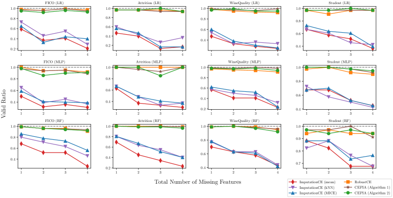
(a) TLPS

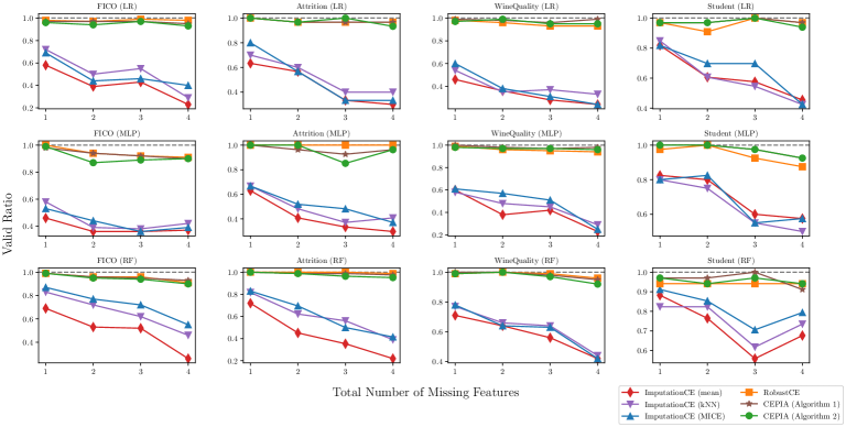
(b) MAD

Figure 5: Experimental results of the valid ratio. The dashed lines indicate 100% validity.

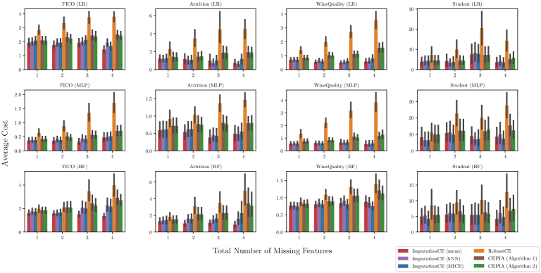
(a) TLPS

(b) MAD

Figure 6: Experimental results of the average cost with 95% confidence intervals.

(a) TLPS

(b) MAD

Figure 7: Experimental results of the average sign agreement score with 95% confidence intervals.

Table 4: Experimental results of the average computational time [s] for TLPS.

Dataset	Method	LR	MLP	RF
FICO	ImputationCE (mean)	0.01741 $\pm$ 0.00747	0.06882 $\pm$ 0.101	0.2173 $\pm$ 0.17
	ImputationCE (kNN)	0.0178 $\pm$ 0.00713	0.07264 $\pm$ 0.0897	0.2123 $\pm$ 0.169
	ImputationCE (MICE)	0.01861 $\pm$ 0.00618	0.073 $\pm$ 0.0864	0.212 $\pm$ 0.165
	RobustCE	0.2228 $\pm$ 0.0269	2.839 $\pm$ 9.18	0.8742 $\pm$ 1.14
	CEPIA (Algorithm 1)	15.69 $\pm$ 4.6	18.59 $\pm$ 11.2	72.83 $\pm$ 21.4
	CEPIA (Algorithm 2)	7.914 $\pm$ 2.46	9.463 $\pm$ 5.49	36.47 $\pm$ 11.3
Attrition	ImputationCE (mean)	0.003619 $\pm$ 0.00388	0.01102 $\pm$ 0.00799	0.04513 $\pm$ 0.0307
	ImputationCE (kNN)	0.003213 $\pm$ 0.00259	0.01181 $\pm$ 0.00709	0.04796 $\pm$ 0.031
	ImputationCE (MICE)	0.002906 $\pm$ 0.00237	0.01161 $\pm$ 0.0072	0.04859 $\pm$ 0.0306
	RobustCE	0.05919 $\pm$ 0.0123	0.09691 $\pm$ 0.0194	0.4899 $\pm$ 0.311
	CEPIA (Algorithm 1)	10.47 $\pm$ 6.49	13.22 $\pm$ 6.87	55.98 $\pm$ 21.4
	CEPIA (Algorithm 2)	5.627 $\pm$ 3.48	6.666 $\pm$ 3.59	28.44 $\pm$ 10.9
WineQuality	ImputationCE (mean)	0.007043 $\pm$ 0.00488	0.03168 $\pm$ 0.0467	0.08812 $\pm$ 0.069
	ImputationCE (kNN)	0.007759 $\pm$ 0.0043	0.03634 $\pm$ 0.0487	0.08638 $\pm$ 0.0749
	ImputationCE (MICE)	0.007842 $\pm$ 0.00436	0.03436 $\pm$ 0.0466	0.08825 $\pm$ 0.0704
	RobustCE	0.08296 $\pm$ 0.0105	0.4082 $\pm$ 0.397	0.5297 $\pm$ 0.473
	CEPIA (Algorithm 1)	3.669 $\pm$ 1.78	7.282 $\pm$ 5.04	43.19 $\pm$ 15.8
	CEPIA (Algorithm 2)	1.934 $\pm$ 0.907	3.715 $\pm$ 2.61	22.54 $\pm$ 8.15
Student	ImputationCE (mean)	0.01213 $\pm$ 0.0093	0.02178 $\pm$ 0.0114	0.00684 $\pm$ 0.00267
	ImputationCE (kNN)	0.001008 $\pm$ 0.000648	0.008517 $\pm$ 0.00853	0.006824 $\pm$ 0.00271
	ImputationCE (MICE)	0.001136 $\pm$ 0.000854	0.008631 $\pm$ 0.00815	0.006547 $\pm$ 0.00246
	RobustCE	0.03567 $\pm$ 0.0597	0.1995 $\pm$ 0.593	0.3643 $\pm$ 0.431
	CEPIA (Algorithm 1)	8.468 $\pm$ 3.92	10.15 $\pm$ 3.59	48.81 $\pm$ 16.9
	CEPIA (Algorithm 2)	4.545 $\pm$ 1.98	5.249 $\pm$ 1.92	25.35 $\pm$ 8.25

Table 5: Experimental results of the average computational time [s] for MAD.

Dataset	Method	LR	MLP	RF
FICO	ImputationCE (mean)	0.01506 $\pm$ 0.00596	0.07742 $\pm$ 0.0817	0.2089 $\pm$ 0.145
	ImputationCE (kNN)	0.01508 $\pm$ 0.00553	0.08782 $\pm$ 0.0874	0.2081 $\pm$ 0.144
	ImputationCE (MICE)	0.01591 $\pm$ 0.00464	0.08784 $\pm$ 0.0799	0.2085 $\pm$ 0.143
	RobustCE	0.07402 $\pm$ 0.0114	1.584 $\pm$ 4.76	0.8329 $\pm$ 0.786
	CEPIA (Algorithm 1)	31.78 $\pm$ 10.5	31.6 $\pm$ 17.7	101.9 $\pm$ 25.3
	CEPIA (Algorithm 2)	17.09 $\pm$ 5.71	17.2 $\pm$ 9.03	52.62 $\pm$ 13.6
Attrition	ImputationCE (mean)	0.009779 $\pm$ 0.00841	0.01076 $\pm$ 0.00766	0.04326 $\pm$ 0.033
	ImputationCE (kNN)	0.002165 $\pm$ 0.00157	0.009435 $\pm$ 0.00524	0.04599 $\pm$ 0.0353
	ImputationCE (MICE)	0.002059 $\pm$ 0.00153	0.009097 $\pm$ 0.00541	0.0453 $\pm$ 0.0332
	RobustCE	0.03529 $\pm$ 0.0112	0.07167 $\pm$ 0.0157	0.4794 $\pm$ 0.335
	CEPIA (Algorithm 1)	29.18 $\pm$ 19.1	30.39 $\pm$ 16.1	81.53 $\pm$ 31.6
	CEPIA (Algorithm 2)	16.2 $\pm$ 10.1	16.25 $\pm$ 8.62	42.71 $\pm$ 16.3
WineQuality	ImputationCE (mean)	0.008271 $\pm$ 0.00577	0.03418 $\pm$ 0.0339	0.08004 $\pm$ 0.0634
	ImputationCE (kNN)	0.007956 $\pm$ 0.00422	0.04058 $\pm$ 0.0415	0.07673 $\pm$ 0.0627
	ImputationCE (MICE)	0.008016 $\pm$ 0.00437	0.03875 $\pm$ 0.0378	0.07822 $\pm$ 0.0551
	RobustCE	0.04863 $\pm$ 0.00794	0.3929 $\pm$ 0.376	0.4919 $\pm$ 0.508
	CEPIA (Algorithm 1)	1.923 $\pm$ 0.899	5.693 $\pm$ 3.81	40.87 $\pm$ 14.4
	CEPIA (Algorithm 2)	0.9915 $\pm$ 0.453	2.873 $\pm$ 1.97	21.33 $\pm$ 7.52
Student	ImputationCE (mean)	0.009595 $\pm$ 0.00915	0.01416 $\pm$ 0.00909	0.007473 $\pm$ 0.00332
	ImputationCE (kNN)	0.0008501 $\pm$ 0.000625	0.006805 $\pm$ 0.00625	0.007583 $\pm$ 0.0035
	ImputationCE (MICE)	0.0008744 $\pm$ 0.000593	0.007364 $\pm$ 0.00698	0.007453 $\pm$ 0.00366
	RobustCE	0.04344 $\pm$ 0.0985	0.2053 $\pm$ 0.607	0.3902 $\pm$ 0.453
	CEPIA (Algorithm 1)	2.795 $\pm$ 1.15	4.325 $\pm$ 1.27	42.11 $\pm$ 14.3
	CEPIA (Algorithm 2)	1.473 $\pm$ 0.571	2.202 $\pm$ 0.695	21.88 $\pm$ 7.06

Table 6: Experimental results on the GiveMeCredit dataset under the MAR and MNAR situations.

Method	MAR			MNAR
	Ratio Valid	Cost	Time [s]	Validity	Cost	Time [s]
ImputationCE (mean)	40.66%	3.095 $\pm$ 3.4	0.004 $\pm$ 0.002	78.20%	4.02 $\pm$ 4.25	0.0042 $\pm$ 0.001
ImputationCE (kNN)	49.45%	3.060 $\pm$ 2.94	0.004 $\pm$ 0.002	83.46%	4.018 $\pm$ 4.18	0.0042 $\pm$ 0.001
ImputationCE (MICE)	47.25%	3.098 $\pm$ 3.19	0.004 $\pm$ 0.002	80.45%	4.016 $\pm$ 4.19	0.0041 $\pm$ 0.001
RobustCE	100.0%	4.002 $\pm$ 4.3	0.030 $\pm$ 0.048	100.0%	4.902 $\pm$ 5.04	0.0308 $\pm$ 0.045
CEPIA (Algorithm 1)	100.0%	3.513 $\pm$ 3.76	2.436 $\pm$ 0.792	100.0%	4.084 $\pm$ 4.33	2.703 $\pm$ 0.744
CEPIA (Algorithm 2)	100.0%	3.495 $\pm$ 3.69	1.241 $\pm$ 0.403	100.0%	4.103 $\pm$ 4.37	1.373 $\pm$ 0.426

(a) TLPS

Method	MAR			MNAR
	Valid Ratio	Cost	Time [s]	Validity	Cost	Time [s]
ImputationCE (mean)	58.70%	1.757 $\pm$ 3.08	0.0034 $\pm$ 0.001	86.36%	1.908 $\pm$ 2.0	0.0036 $\pm$ 0.001
ImputationCE (kNN)	66.30%	1.755 $\pm$ 3.03	0.0036 $\pm$ 0.002	89.39%	1.914 $\pm$ 1.95	0.0037 $\pm$ 0.001
ImputationCE (MICE)	61.96%	1.735 $\pm$ 3.05	0.0034 $\pm$ 0.001	87.88%	1.882 $\pm$ 1.93	0.0037 $\pm$ 0.001
RobustCE	98.91%	2.076 $\pm$ 3.14	0.0594 $\pm$ 0.025	100.0%	2.165 $\pm$ 2.02	0.0567 $\pm$ 0.026
CEPIA (Algorithm 1)	100.0%	1.852 $\pm$ 3.07	2.859 $\pm$ 0.755	100.0%	1.879 $\pm$ 1.95	2.989 $\pm$ 0.643
CEPIA (Algorithm 2)	100.0%	1.856 $\pm$ 3.09	1.429 $\pm$ 0.419	100.0%	1.887 $\pm$ 1.95	1.509 $\pm$ 0.361

(b) MAD

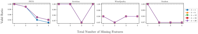
(a) Valid Ratio

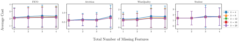
(b) Cost

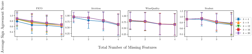
(c) Sign Agreement Score

Figure 10: Experimental results of the sensitivity analyses on the parameter $k$ for MAD.

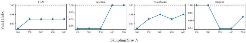
(a) Valid Ratio

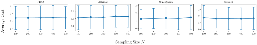
(b) Cost

(c) Sign Agreement Score

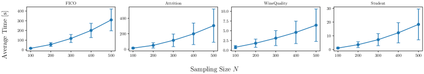
(d) Computational Time

Figure 12: Experimental results of the sensitivity analyses on the sampling size $N$ for MAD.

References

- Ahmad et al. [2019] M. A. Ahmad, C. Eckert, and A. Teredesai. The challenge of imputation in explainable artificial intelligence models. In Proceedings of the Workshop on Artificial Intelligence Safety 2019, 2019.
- Aivodji et al. [2020] U. Aivodji, A. Bolot, and S. Gambs. Model extraction from counterfactual explanations. arXiv, arXiv:2009.01884, 2020.
- Ayme et al. [2022] A. Ayme, C. Boyer, A. Dieuleveut, and E. Scornet. Near-optimal rate of consistency for linear models with missing values. In Proceedings of the 39th International Conference on Machine Learning, pages 1211–1243, 2022.
- Badanidiyuru et al. [2014] A. Badanidiyuru, B. Mirzasoleiman, A. Karbasi, and A. Krause. Streaming submodular maximization: Massive data summarization on the fly. In Proceedings of the 20th ACM SIGKDD International Conference on Knowledge Discovery and Data Mining, pages 671–680, 2014.
- Barocas et al. [2020] S. Barocas, A. D. Selbst, and M. Raghavan. The hidden assumptions behind counterfactual explanations and principal reasons. In Proceedings of the 2020 Conference on Fairness, Accountability, and Transparency, pages 80–89, 2020.
- Bertsimas et al. [2021] D. Bertsimas, A. Delarue, and J. Pauphilet. Prediction with missing data. arXiv, arXiv:2104.03158, 2021.
- Cesa-Bianchi et al. [2011] N. Cesa-Bianchi, S. Shalev-Shwartz, and O. Shamir. Efficient learning with partially observed attributes. Journal of Machine Learning Research, 12(87):2857–2878, 2011.
- Cui et al. [2015] Z. Cui, W. Chen, Y. He, and Y. Chen. Optimal action extraction for random forests and boosted trees. In Proceedings of the 21th ACM SIGKDD International Conference on Knowledge Discovery and Data Mining, pages 179–188, 2015.
- Dick et al. [2008] U. Dick, P. Haider, and T. Scheffer. Learning from incomplete data with infinite imputations. In Proceedings of the 25th International Conference on Machine Learning, pages 232–239, 2008.
- Dominguez-Olmedo et al. [2022] R. Dominguez-Olmedo, A. H. Karimi, and B. Schölkopf. On the adversarial robustness of causal algorithmic recourse. In Proceedings of the 39th International Conference on Machine Learning, pages 5324–5342, 2022.
- Dua and Graff [2017] D. Dua and C. Graff. UCI machine learning repository. http://archive.ics.uci.edu/ml, 2017. Accessed: 2023-01-26.
- Dutta et al. [2022] S. Dutta, J. Long, S. Mishra, C. Tilli, and D. Magazzeni. Robust counterfactual explanations for tree-based ensembles. In Proceedings of the 39th International Conference on Machine Learning, pages 5742–5756, 2022.
- FICO et al. [2018] FICO, Google, Imperial College London, MIT, University of Oxford, UC Irvine, and UC Berkeley. Explainable Machine Learning Challenge. https://community.fico.com/s/explainable-machine-learning-challenge, 2018. Accessed: 2023-01-26.
- Guidotti [2022] R. Guidotti. Counterfactual explanations and how to find them: literature review and benchmarking. Data Mining and Knowledge Discovery, 2022.
- Hancox-Li [2020] L. Hancox-Li. Robustness in machine learning explanations: Does it matter? In Proceedings of the 2020 Conference on Fairness, Accountability, and Transparency, pages 640–647, 2020.
- Harshaw et al. [2022] C. Harshaw, E. Kazemi, M. Feldman, and A. Karbasi. The power of subsampling in submodular maximization. Mathematics of Operations Research, 47(2):1365–1393, 2022.
- Ipsen et al. [2022] N. B. Ipsen, P.-A. Mattei, and J. Frellsen. How to deal with missing data in supervised deep learning? In Proceedings of the 10th International Conference on Learning Representations, 2022.
- Jeong et al. [2022] H. Jeong, H. Wang, and F. P. Calmon. Fairness without imputation: A decision tree approach for fair prediction with missing values. In Proceedings of the 36th AAAI Conference on Artificial Intelligence, pages 9558–9566, 2022.
- Josse et al. [2019] J. Josse, N. Prost, E. Scornet, and G. Varoquaux. On the consistency of supervised learning with missing values. arXiv, arXiv:1902.06931, 2019.
- Kaggle [2011] Kaggle. Give Me Some Credit | Kaggle. https://www.kaggle.com/c/GiveMeSomeCredit/, 2011. Accessed: 2023-01-26.
- Kaggle [2017] Kaggle. IBM HR Analytics Employee Attrition & Performance. https://www.kaggle.com/pavansubhasht/ibm-hr-analytics-attrition-dataset, 2017. Accessed: 2023-01-26.
- Kanamori et al. [2020] K. Kanamori, T. Takagi, K. Kobayashi, and H. Arimura. DACE: Distribution-aware counterfactual explanation by mixed-integer linear optimization. In Proceedings of the 29th International Joint Conference on Artificial Intelligence, pages 2855–2862, 2020.
- Kanamori et al. [2021] K. Kanamori, T. Takagi, K. Kobayashi, Y. Ike, K. Uemura, and H. Arimura. Ordered counterfactual explanation by mixed-integer linear optimization. In Proceedings of the 35th AAAI Conference on Artificial Intelligence, pages 11564–11574, 2021.
- Kanamori et al. [2022] K. Kanamori, T. Takagi, K. Kobayashi, and Y. Ike. Counterfactual explanation trees: Transparent and consistent actionable recourse with decision trees. In Proceedings of the 25th International Conference on Artificial Intelligence and Statistics, pages 1846–1870, 2022.
- Karimi et al. [2020a] A.-H. Karimi, G. Barthe, B. Balle, and I. Valera. Model-agnostic counterfactual explanations for consequential decisions. In Proceedings of the 23rd International Conference on Artificial Intelligence and Statistics, pages 895–905, 2020a.
- Karimi et al. [2020b] A.-H. Karimi, J. von Kügelgen, B. Schölkopf, and I. Valera. Algorithmic recourse under imperfect causal knowledge: a probabilistic approach. In Proceedings of the 34th International Conference on Neural Information Processing Systems, pages 265–277, 2020b.
- Karimi et al. [2021] A.-H. Karimi, B. Schölkopf, and I. Valera. Algorithmic recourse: From counterfactual explanations to interventions. In Proceedings of the 2021 ACM Conference on Fairness, Accountability, and Transparency, pages 353–362, 2021.
- Krishna et al. [2022] S. Krishna, T. Han, A. Gu, J. Pombra, S. Jabbari, S. Wu, and H. Lakkaraju. The disagreement problem in explainable machine learning: A practitioner’s perspective. arXiv, arXiv:2202.01602, 2022.
- Le Morvan et al. [2021] M. Le Morvan, J. Josse, E. Scornet, and G. Varoquaux. What’s a good imputation to predict with missing values? In Proceedings of the 35th International Conference on Neural Information Processing Systems, pages 11530–11540, 2021.
- Ley et al. [2022] D. Ley, U. Bhatt, and A. Weller. Diverse, global and amortised counterfactual explanations for uncertainty estimates. In Proceedings of the 36th AAAI Conference on Artificial Intelligence, pages 7390–7398, 2022.
- Little and Rubin [2019] R. J. A. Little and D. B. Rubin. Statistical Analysis with Missing Data. John Wiley & Sons, Inc., 3rd edition, 2019.
- Lucic et al. [2022] A. Lucic, H. Oosterhuis, H. Haned, and M. de Rijke. FOCUS: Flexible optimizable counterfactual explanations for tree ensembles. In Proceedings of the 36th AAAI Conference on Artificial Intelligence, pages 5313–5322, 2022.
- Ma and Zhang [2021] C. Ma and C. Zhang. Identifiable generative models for missing not at random data imputation. In Proceedings of the 35th International Conference on Neural Information Processing Systems, pages 27645–27658, 2021.
- Marques-Silva et al. [2021] J. Marques-Silva, T. Gerspacher, M. C. Cooper, A. Ignatiev, and N. Narodytska. Explanations for monotonic classifiers. In Proceedings of the 38th International Conference on Machine Learning, pages 7469–7479, 2021.
- Mattei and Frellsen [2019] P.-A. Mattei and J. Frellsen. MIWAE: Deep generative modelling and imputation of incomplete data sets. In Proceedings of the 36th International Conference on Machine Learning, pages 4413–4423, 2019.
- Miller [2019] T. Miller. Explanation in artificial intelligence: Insights from the social sciences. Artificial Intelligence, 267:1–38, 2019.
- Milli et al. [2019] S. Milli, L. Schmidt, A. D. Dragan, and M. Hardt. Model reconstruction from model explanations. In Proceedings of the Conference on Fairness, Accountability, and Transparency, pages 1–9, 2019.
- Mohri et al. [2012] M. Mohri, A. Rostamizadeh, and A. Talwalkar. Foundations of Machine Learning. The MIT Press, 2012.
- Mothilal et al. [2020] R. K. Mothilal, A. Sharma, and C. Tan. Explaining machine learning classifiers through diverse counterfactual explanations. In Proceedings of the 2020 Conference on Fairness, Accountability, and Transparency, pages 607–617, 2020.
- Murray [2018] J. S. Murray. Multiple Imputation: A Review of Practical and Theoretical Findings. Statistical Science, 33(2):142–159, 2018.
- Nemhauser et al. [1978] G. L. Nemhauser, L. A. Wolsey, and M. L. Fisher. An analysis of approximations for maximizing submodular set functions—i. Mathematical Programming, 14(1):265–294, 1978.
- Parmentier and Vidal [2021] A. Parmentier and T. Vidal. Optimal counterfactual explanations in tree ensembles. In Proceedings of the 38th International Conference on Machine Learning, pages 8422–8431, 2021.
- Pawelczyk et al. [2020] M. Pawelczyk, K. Broelemann, and G. Kasneci. Learning model-agnostic counterfactual explanations for tabular data. In Proceedings of The Web Conference 2020, pages 3126–3132, 2020.
- Pawelczyk et al. [2022a] M. Pawelczyk, C. Agarwal, S. Joshi, S. Upadhyay, and H. Lakkaraju. Exploring counterfactual explanations through the lens of adversarial examples: A theoretical and empirical analysis. In Proceedings of the 25th International Conference on Artificial Intelligence and Statistics, pages 4574–4594, 2022a.
- Pawelczyk et al. [2022b] M. Pawelczyk, T. Datta, J. van-den Heuvel, G. Kasneci, and H. Lakkaraju. Probabilistically robust recourse: Navigating the trade-offs between costs and robustness in algorithmic recourse. arXiv, arXiv:2203.06768, 2022b.
- Pearson [2006] R. K. Pearson. The problem of disguised missing data. ACM SIGKDD Explorations Newsletter, 8(1):83–92, 2006.
- Rawal and Lakkaraju [2020] K. Rawal and H. Lakkaraju. Beyond individualized recourse: Interpretable and interactive summaries of actionable recourses. In Proceedings of the 34th International Conference on Neural Information Processing Systems, pages 12187–12198, 2020.
- Ribeiro et al. [2016] M. T. Ribeiro, S. Singh, and C. Guestrin. “Why Should I Trust You?”: Explaining the predictions of any classifier. In Proceedings of the 22nd ACM SIGKDD International Conference on Knowledge Discovery and Data Mining, pages 1135–1144, 2016.
- Rubin [1976] D. B. Rubin. Inference and missing data. Biometrika, 63(3):581–592, 1976.
- Rubin [1987] D. B. Rubin. Multiple imputation for nonresponse in surveys, volume 81. John Wiley & Sons, Inc., 1987.
- Saar-Tsechansky and Provost [2007] M. Saar-Tsechansky and F. Provost. Handling missing values when applying classification models. Journal of Machine Learning Research, 8:1623–1657, 2007.
- Schenker et al. [2006] N. Schenker, T. E. Raghunathan, P.-L. Chiu, D. M. Makuc, G. Zhang, and A. J. Cohen. Multiple imputation of missing income data in the national health interview survey. Journal of the American Statistical Association, 101(475):924–933, 2006.
- Serra et al. [2018] T. Serra, C. Tjandraatmadja, and S. Ramalingam. Bounding and counting linear regions of deep neural networks. In Proceedings of the 35th International Conference on Machine Learning, pages 4558–4566, 2018.
- Slack et al. [2021] D. Slack, S. Hilgard, H. Lakkaraju, and S. Singh. Counterfactual Explanations Can Be Manipulated. In Proceedings of the 35th International Conference on Neural Information Processing Systems, pages 62–75, 2021.
- Troyanskaya et al. [2001] O. Troyanskaya, M. Cantor, G. Sherlock, P. Brown, T. Hastie, R. Tibshirani, D. Botstein, and R. B. Altman. Missing value estimation methods for dna microarrays. Bioinformatics, 17(6):520–525, 2001.
- Ustun et al. [2019] B. Ustun, A. Spangher, and Y. Liu. Actionable recourse in linear classification. In Proceedings of the 2019 Conference on Fairness, Accountability, and Transparency, pages 10–19, 2019.
- van Buuren and Groothuis-Oudshoorn [2011] S. van Buuren and K. Groothuis-Oudshoorn. mice: Multivariate imputation by chained equations in R. Journal of Statistical Software, 45(3):1–67, 2011.
- Venkatasubramanian and Alfano [2020] S. Venkatasubramanian and M. Alfano. The philosophical basis of algorithmic recourse. In Proceedings of the 2020 Conference on Fairness, Accountability, and Transparency, pages 284–293, 2020.
- Verma et al. [2020] S. Verma, V. Boonsanong, M. Hoang, K. E. Hines, J. P. Dickerson, and C. Shah. Counterfactual explanations and algorithmic recourses for machine learning: A review. arXiv, arXiv:2010.10596, 2020.
- von Kügelgen et al. [2022] J. von Kügelgen, A.-H. Karimi, U. Bhatt, I. Valera, A. Weller, and B. Schölkopf. On the fairness of causal algorithmic recourse. In Proceedings of the 36th AAAI Conference on Artificial Intelligence, pages 9584–9594, 2022.
- Wachter et al. [2018] S. Wachter, B. Mittelstadt, and C. Russell. Counterfactual explanations without opening the black box: Automated decisions and the GDPR. Harvard Journal of Law & Technology, 31:841–887, 2018.
- Wang et al. [2022] Y. Wang, H. Qian, and C. Miao. Dualcf: Efficient model extraction attack from counterfactual explanations. In Proceedings of the 2022 ACM Conference on Fairness, Accountability, and Transparency, pages 1318–1329, 2022.
- Yoon et al. [2018] J. Yoon, J. Jordon, and M. van der Schaar. GAIN: Missing data imputation using generative adversarial nets. In Proceedings of the 35th International Conference on Machine Learning, pages 5689–5698, 2018.
- Zhang and Long [2021] Y. Zhang and Q. Long. Assessing Fairness in the Presence of Missing Data. In Proceedings of the 35th International Conference on Neural Information Processing Systems, pages 16007–16019, 2021.
- Zhao and Udell [2020] Y. Zhao and M. Udell. Missing value imputation for mixed data via gaussian copula. In Proceedings of the 26th ACM SIGKDD International Conference on Knowledge Discovery and Data Mining, pages 636–646, 2020.