A Manifold Learning-based CSI Feedback Framework for FDD Massive MIMO

Abstract

Massive multi-input multi-output (MIMO) in Frequency Division Duplex (FDD) mode suffers from heavy feedback overhead for Channel State Information (CSI). In this paper, a novel manifold learning-based CSI feedback framework (MLCF) is proposed to reduce the feedback and improve the spectral efficiency of FDD massive MIMO. Manifold learning (ML) is an effective method for dimensionality reduction. However, most ML algorithms focus only on data compression, and lack the corresponding recovery methods. Moreover, the computational complexity is high when dealing with incremental data. To solve these problems, we propose a landmark selection algorithm to characterize the topological skeleton of the manifold where the CSI sample resides. Based on the learned skeleton, the local patch of the incremental CSI on the manifold can be easily determined by its nearest landmarks. This motivates us to propose a low-complexity compression and reconstruction scheme by keeping the local geometric relationships with landmarks unchanged. We theoretically prove the convergence of the proposed algorithm. Meanwhile, the upper bound on the error of approximating the CSI samples using landmarks is derived. Simulation results under an industrial channel model of 3GPP demonstrate that the proposed MLCF method outperforms existing algorithms based on compressed sensing and deep learning.

I Introduction

Massive multiple-input multiple-output (MIMO) is one of the key enabling technologies for the fifth generation (5G) wireless communication systems [2] [3]. By deploying a large number of antennas at the base station (BS) side, massive MIMO systems have the potential to provide high spectral and energy efficiency [4]. These performance gains depend on accurate and timely channel state information (CSI) at the transmitter. Since full channel reciprocity is not available in the frequency division duplex (FDD) system, the downlink CSI has to be estimated from pilots at the user equipment (UE) side and then fed back to the BS [5] [6]. Unfortunately, the dimension of the channel matrix scales with the number of BS antennas, which exacerbates the feedback overhead in massive MIMO systems [7]. In addition, the amount of feedback is constrained by the coherence time and coherence bandwidth of the channel, both of which are limited in a mobility environment with multipath components. Therefore, one of the most challenging tasks for FDD massive MIMO is how to reduce the CSI feedback overhead while keeping the accuracy of the reconstructed CSI at the BS high.

The urgent demand for limited CSI feedback has motivated extensive research. [8] and [9] attempt to share a vector quantization codebook between the BS and the UE. The UE delivers back the index of the codeword that best matches the downlink CSI. The size of the codebook required to maintain the level of communication quality grows exponentially with the number of antennas, which is costly in the case of massive MIMO. In view of the sparsity of massive MIMO channels in a certain transform domain, the theory of compressed sensing (CS) is also introduced in [10] [11]. Such approaches rely on the sparse assumption of the channel, which may not always be present in practice. Moreover, iterative algorithms are proposed for CSI recovery, resulting in heavy computational costs. In particular, some works [12] [13] parameterize the azimuth angle of arrival (AoA) and the angle of departure (AoD) to display the sparsity of the channel matrix. Overcomplete dictionaries are designed to approximate the steering vectors related to the arrival and departure angles. To guarantee high resolution for AoA and AoD, the size of dictionaries is typically so large that the memory cost is high. As with CS techniques, there is still the issue of reconstruction complexity.

Due to the powerful feature extraction ability, deep learning (DL) has recently shown great potential in the field of wireless communication, such as hybrid precoding [14] and channel prediction [15]. This has also inspired a number of DL-based algorithms to address the problem of limited CSI feedback in FDD massive MIMO systems. An auto-encoder network named CsiNet [16] has been proposed for CSI compression and recovery, which improves the reconstruction quality and computation speed. Specifically, an encoder compresses the channel matrices into codewords at the UE, and then a decoder reconstructs the channel matrices from the received codewords at the BS. Enlightened by the fact that DL is an appealing method for CSI feedback, a multi-resolution CRBlock [17] is designed to improve the robustness under various scenarios and compression ratios. Meanwhile, a novel network training method called warm-up aided cosine learning rate scheduler is also proposed to boost the reconstruction performance of the network. The temporal correlation of CSI in adjacent time slots is extracted by the long short-term memory (LSTM) network [18] to further improve the reconstruction quality. In fact, there is a bottleneck of excessive parameters in neural networks. To address this bottleneck, [19] suggests a lightweight network that still shows good reconstruction performance. Nevertheless, the reconstruction qualities of the aforementioned DL-based algorithms are limited at low compression ratios.

In this paper, we revisit the problem of limited CSI feedback in FDD massive MIMO systems by means of manifold learning (ML) [20, 21, 22]. The previous research mainly focused on the characteristics of the channel structure in the angular-delay/frequency domain [16][23] or the structure of the channel covariance matrix [24, 25, 26]. The intrinsic manifold structure where the CSI samples reside is neglected. As a dimensionality reduction approach, ML can map a high-dimensional data set into a low-dimensional space while preserving the intrinsic manifold structure in the data. However, two open issues hinder ML from being applied in practice. First, most ML algorithms, such as Locally Linear Embedding (LLE) [21] and Local Tangent Space Alignment (LTSA) [22], work in a “batch” mode, which means that dimensionality reduction cannot be performed in an incremental way. Whenever a new sample is added, the data set needs to be updated to incorporate it, and the low-dimensional embeddings of all samples have to be recalculated simultaneously. This process undoubtedly increases the computational cost. Second, most ML algorithms lack an inverse mapping from the low-dimensional embedding to the high-dimensional data, i.e., they focus on data compression, while the corresponding reconstruction methods are not provided. Some algorithms [22] [27] attempt to recover the original data by introducing kernel regression functions to fit the high-dimensional data. Since the number of required kernel functions scales linearly with the dimension of the high-dimensional data, determining the parameters of these functions might be challenging when the dimension of the data is large.

In order to address the aforementioned issues in traditional ML approaches and adopt the idea of ML to limited feedback, we propose a novel ML-based CSI feedback framework (MLCF) to improve the spectral efficiency (SE) of FDD massive MIMO systems. It is assumed that the CSI sample lie on a smooth, low-dimensional manifold embedded in a high-dimensional space. Without prior knowledge of the intrinsic manifold, a data set consisting of high-density CSI samples is constructed to characterize the manifold. It may contain spatially redundant samples, thus we select representative landmarks from the data set to describe the manifold skeleton. At this point, for the newly sampled CSI, its local patch on the manifold can be easily identified by its nearest neighbors in the landmarks. The incremental CSI can then be compressed by preserving the local geometric relationships with the landmarks rather than the data set. This principle is also applied to reconstruct the original CSI.

The main contributions of this paper are summarized as follows:

1. To the best of our knowledge, this paper is the first to adopt manifold learning to the problem of limited CSI feedback. We propose a novel landmark selection method to characterize the topological skeleton of the manifold where the CSI samples reside. An alternating iteration optimization algorithm is proposed to select representative landmarks. Meanwhile, the closed-form solutions of the algorithm are provided.

2. By exploiting the intrinsic structure of the manifold, we propose a low-complexity compression and reconstruction scheme for the incremental CSI. The key idea is to keep the local geometric relationships between the incremental CSI and the landmarks unchanged.

3. We prove the convergence of the proposed alternating iterative optimization algorithm, and show that the value of the objective function decreases monotonically in each iteration.

4. We derive an upper bound on the error of approximating the CSI with landmarks. We show the main factors that affect the error are the number and correctness of the nearest neighbors in the landmarks. If all neighbors lie in a sufficiently compact region, the approximation error is quite small.

Simulation results under the industrial channel model of 3GPP demonstrate large gains in terms of the normalized mean square error (NMSE) of the reconstructed CSI. In particular, when the compression ratio is 1/32, the proposed MLCF method brings a gain of at least 25 dB compared with existing CS-based or DL-based methods.

Notations: We use boldface to denote vectors and matrices. $({\mathbf{A}})^{T}$ and $({\mathbf{A}})^{H}$ denote the transpose and conjugate transpose of the matrix ${\mathbf{A}}$, respectively. ${\mathop{\Re}\nolimits}\{\cdot\}$ and ${\mathop{\Im}\nolimits}\{\cdot\}$ represent the real and imaginary parts of a matrix, respectively. ${\|\cdot\|}_{2}$ is the Euclidean norm of a vector, and ${\|\cdot\|}_{F}$ is the Frobenius norm of a matrix. ${\mathbf{A}}\otimes{\mathbf{B}}$ denotes the Kronecker product of matrices ${\mathbf{A}}$ and ${\mathbf{B}}$. $\rm{tr}\{\cdot\}$ denotes the trace of a square matrix. ${\boldsymbol{e}}\in{\mathbb{R}^{k\times 1}}$ is a column vector in which all elements are ones. ${{\boldsymbol{A}}_{i*}}$ is the $i$-th row of the matrix ${\boldsymbol{A}}$. $span(\boldsymbol{A})$ denotes the column space of $\boldsymbol{A}$. ${\rm{diag}}({q_{1}},{q_{2}},\cdots,{q_{n}})$ represents a diagonal matrix with ${q_{1}},{q_{2}},\cdots,{q_{n}}$ at the main diagonal. ${\mathbb{E}}\{\cdot\}$ denotes the expectation.

II System Model

Consider a cellular FDD massive MIMO system, whereby a BS services multiple single-antenna UEs simultaneously. The BS is equipped with a uniform planar array (UPA) with $N_{v}$ rows and $N_{h}$ columns, and there are ${N_{t}}={N_{v}}{N_{h}}$ antennas in total. The system operates in orthogonal frequency division multiplexing (OFDM) over $N_{f}$ subcarriers.

For ease of exposition, we focus on an arbitrary UE in a certain cell. The received signal at the $i$-th subcarrier is

$${r_{i}}={\boldsymbol{h}_{i}}{\boldsymbol{p}_{i}}{s_{i}}+{n_{i}},$$ (1)

where ${\boldsymbol{h}_{i}}\in\mathbb{C}^{1\times{N_{t}}}$, ${\boldsymbol{p}_{i}}\in\mathbb{C}^{{N_{t}}\times 1}$, ${s_{i}}\in\mathbb{C}$, and ${n_{i}}\in\mathbb{C}$ denote the downlink channel vector, the precoding vector, the transmit data symbol, and the additive noise at the $i$-th subcarrier, respectively. Operating in FDD mode, the transmitter needs to know the accurate and instantaneous downlink CSI to achieve high SE.

In this work, the clustered delay line (CDL) channel model is adopted, conformed to the 3GPP TR 38.901 specifications [28]. There exists $N_{\rm{cl}}$ scattering clusters in the propagation environment, each of which contains $N_{\rm{ray}}$ rays. Based on this assumption, the downlink channel vector between the BS antennas and the UE antenna at the certain frequency $f_{i}$ and time $t$ is modeled as

$$\begin{array}[]{l}{\boldsymbol{h}_{f_{i}}}=\sum\limits_{n=1}^{N_{\rm{cl}}}{\sum\limits_{m=1}^{N_{\rm{ray}}}{{\alpha_{n,m}}{\textbf{a}_{\rm{tx}}^{H}(\theta_{n,m}^{\rm{tx}},\phi_{n,m}^{\rm{tx}})}{e^{-j2\pi{f_{i}}{\tau_{n,m}}}}{e^{j{w_{n,m}}t}}}}\end{array},$$ (2)

where ${\alpha_{n,m}}$, ${\tau_{n,m}}$ and ${w_{n,m}}$ are the channel gain, the time delay, and the Doppler frequency of the $m$-th ray in the $n$-th cluster, respectively. Besides, ${\textbf{a}_{\rm{tx}}(\theta,\phi)}$ is the 3D steering vector of the antenna array at the transmitter with a zenith angle of departure ${\theta}$ and an azimuth angle of departure ${\phi}$. Taking into account that the UPA is positioned on the YZ plane, the 3D steering vector is [29]

$$\textbf{a}(\theta,\phi)={\textbf{a}_{h}}(\theta,\phi)\otimes{\textbf{a}_{v}}(\theta),$$ (3)

where

$${\textbf{a}_{h}}(\theta,\phi)=\left[{\begin{array}[]{*{20}{c}}{\rm{1}}\\ {{e^{j2\pi\frac{{{D_{h}}\sin\theta\sin\phi}}{{{\lambda_{0}}}}}}}\\ \vdots\\ {{e^{j2\pi\frac{{({N_{h}}-1){D_{h}}\sin\theta\sin\phi}}{{{\lambda_{0}}}}}}}\end{array}}\right],$$ (4)

and

$${\textbf{a}_{v}}(\theta)=\left[{\begin{array}[]{*{20}{c}}{\rm{1}}\\ {{e^{j2\pi\frac{{{D_{v}}\cos\theta}}{{{\lambda_{0}}}}}}}\\ \vdots\\ {{e^{j2\pi\frac{{({N_{v}}-1){D_{v}}\cos\theta}}{{{\lambda_{0}}}}}}}\end{array}}\right],$$ (5)

with ${D_{v}}$, ${D_{h}}$ and ${\lambda_{0}}$ being the vertical and horizontal spacing between element antennas and the central carrier wavelength, respectively.

We integrate the channel vectors over $N_{f}$ subcarriers into a wideband channel matrix ${\mathbf{H}}(t)\in{\mathbb{R}^{{N_{f}}\times{N_{t}}}}$ as

$${\mathbf{H}}(t)=\left[{\begin{array}[]{*{20}{c}}{\boldsymbol{h}_{f_{1}}^{T}}&{\boldsymbol{h}_{f_{2}}^{T}}&\cdots&{\boldsymbol{h}_{f_{N_{f}}}^{T}}\end{array}}\right]^{T}.$$ (6)

Given that ML only supports the calculation of real values, the complex channel matrix ${\mathbf{H}}(t)$ has to be decomposed into real and imaginary parts, which are stacked as below

$$\widetilde{\mathbf{H}}(t)=\left[{\begin{array}[]{*{20}{c}}{{\mathop{\Re}\nolimits}\left\{{{\mathbf{H}}(t)}\right\}}\\ {{\mathop{\Im}\nolimits}\left\{{{\mathbf{H}}(t)}\right\}}\end{array}}\right]\in{\mathbb{R}^{2{N_{f}}\times{N_{t}}}}.$$ (7)

Suppose that the real CSI is sampled from a high-dimensional manifold. The manifold topology can be characterized by a data set consisting of high-density samples on the manifold. However, the large-scale data set may lead to high computational complexity in addition to spatially redundant samples. To simplify the process of ML, we introduce representative landmarks to replace the data set.

In details, the UE compresses the downlink CSI estimated from the pilot signals into its low-dimensional embedding by means of manifold learning

$$\boldsymbol{Y}=f(\mathbf{H},\boldsymbol{D}_{\rm{H}}^{\rm{dr}},\boldsymbol{D}_{\rm{L}}^{\rm{dr}}),$$ (8)

where $f(\cdot)$ denotes the compression function, $\boldsymbol{D}_{\rm{H}}^{\rm{dr}}$ and $\boldsymbol{D}_{\rm{L}}^{\rm{dr}}$ are a set of dictionaries for dimensionality reduction, consisting of landmarks. After receiving $\boldsymbol{Y}$, the reconstruction operation is performed at the BS to recover the original downlink CSI

$$\mathbf{\hat{H}}=g(\boldsymbol{Y},\boldsymbol{D}_{\rm{H}}^{\rm{rc}},\boldsymbol{D}_{\rm{L}}^{\rm{rc}}),$$ (9)

where $g(\cdot)$ is the reverse operation of compression, $\boldsymbol{D}_{\rm{H}}^{\rm{rc}}$ and $\boldsymbol{D}_{\rm{L}}^{\rm{rc}}$ are a set of reconstruction dictionaries. Note that these two sets of dictionaries are learned in advance.

III Proposed Landmark Selection Method for Manifold Learning

III-A An overview of manifold learning

It is common to observe high-dimensional data samples with low intrinsic degrees of freedom in real-world systems. Access to abundant samples is beneficial for an algorithm attempting to extract features from the data. Frustratingly, the high-dimensional data suffers from the curse of dimensionality, exacerbating storage requirements and computational burden. A typical strategy to alleviate this problem is dimensionality reduction, which aims to map a high-dimensional data set into a low-dimensional space while maintaining the underlying structure in the data.

As an efficient dimensionality reduction approach, manifold learning has drawn a lot of attention due to its nonlinear property. It assumes that the data samples reside on a low-dimensional manifold embedded in a high-dimensional space. Intuitively, each sample on the manifold has a local neighborhood that is homeomorphic to Euclidean space. Although the high-dimensional manifold has a complicated structure, it is locally similar to Euclidean space. Therefore, it is possible to obtain a local mapping relationship between the high-dimensional space and the low-dimensional manifold, and then extend the local relationship to the global space. Based on this idea, the high-dimensional data can be compressed to any dimension, especially 2D or 3D for visual analysis. Despite the global optimization functions designed to obtain the low-dimensional embeddings differ among various ML methods, most of them involve the construction of local neighborhoods. The common strategies for neighborhood selection fall into two categories: $k$-nearest neighbor (kNN) and $\epsilon$-neighborhood. In this paper, the former is adopted to select the neighbors.

In FDD massive MIMO systems, a total of ${T_{s}}$ downlink CSI samples are observed to form a high-dimensional data set

$${\boldsymbol{X}}=\left[{\begin{array}[]{*{20}{c}}\widetilde{\mathbf{H}}(1)&\cdots&\widetilde{\mathbf{H}}(T_{s})\end{array}}\right].$$ (10)

For simplicity, let ${{\boldsymbol{x}}_{i}}$ be the $i$-th column of ${\boldsymbol{X}}\in{\mathbb{R}^{2{N_{f}}\times N}}$, and $N={N_{t}}{T_{s}}$ be the size of ${\boldsymbol{X}}$. To satisfy the ML assumption, we consider ${{\boldsymbol{x}}_{i}}\in{\mathbb{R}^{2{N_{f}}\times 1}}$ residing on a $d$-dimensional manifold $\mathcal{S}$ embedded in a $2{N_{f}}$-dimensional space $\mathcal{M}$. Since we have no access to the true manifold, abundant CSI samples are collected to construct the data set ${\boldsymbol{X}}$ representing the high-dimensional space $\mathcal{M}$. As for the low-dimensional manifold $\mathcal{S}$, it is characterized by the low-dimensional embedding of ${\boldsymbol{X}}$. The process of dimensionality reduction is expressed as

$${{\boldsymbol{y}}_{i}}=f\left({{\boldsymbol{x}}_{i}}\right)+{{\boldsymbol{\epsilon}}_{i}},$$ (11)

where ${f:\mathcal{M}\rightarrow\mathcal{S}}$ is the compression function, ${{\boldsymbol{\epsilon}}_{i}}\in{\mathbb{R}^{d\times 1}}$ is the noise, and the low-dimensional embedding of ${\boldsymbol{X}}$ is denoted by ${\boldsymbol{Y}}=\left[{\begin{array}[]{*{20}{c}}{{\boldsymbol{y}}_{1}}&{{\boldsymbol{y}}_{2}}&\cdots&{{\boldsymbol{y}}_{N}}\end{array}}\right]$ $\in{\mathbb{R}^{d\times N}}$. Obviously, the compression ratio can be defined as

$$\gamma=\frac{d}{2{N_{f}}},$$ (12)

where $d\ll 2{N_{f}}$.

In short, given a high-dimensional data set ${\boldsymbol{X}}$, the task of ML is to obtain its low-dimensional representation ${\boldsymbol{Y}}$ while finding out the mapping function $f$. In contrast, data reconstruction, the inverse process of dimensionality reduction, aims to recover the original high-dimensional data from the low-dimensional embedding while obtaining the reconstruction mapping ${g:\mathcal{S}\rightarrow\mathcal{M}}$. Once the explicit functions $f$ and $g$ are known, the newly sampled CSI can be efficiently compressed and reconstructed.

III-B Landmark selection

It should be noted that the dimensionality and the number of data samples directly affect the complexity of most ML methods. Typically, the low-dimensional embedding is obtained by performing an eigenvector analysis on the data similarity matrix, whose size is $N\times N$. As a result, ML is inconvenient for large-scale data sets, which demand excessive computational and storage resources. Considerable efforts have been devoted to deal with the case of large data sets. The idea of perfectly approximating the manifold skeleton with a collection of landmarks [30] emerges, however selecting the right landmarks is essential. This also motivates us to employ landmarks to solve the problem of incremental feedback. As there is no prior knowledge of the intrinsic manifold structure, the representative landmarks are selected from the historical CSI data set to characterize the topological skeleton of the manifold. The main principle is that the selected landmarks can linearly approximate all samples on the manifold with minimal error. For the incremental CSI, its local patch on the manifold can be easily determined with the known landmarks (see Fig. 1 for an illustration).

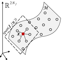
(a)

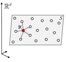
(b)

Figure 1: An illustration of the high-dimensional manifold (a) and the corresponding low-dimensional embedding (b). The CSI data points are sampled from the surface in (a). $span({\boldsymbol{J}}_{g}({{\boldsymbol{y}}_{i}}))$ is the tangent space at the sample ${{\boldsymbol{x}}_{i}}$ (the solid circle). The hollow circles are the landmarks learned by our proposed Algorithm 1. The local geometric relation between ${{\boldsymbol{x}}_{i}}$ and its nearest landmarks remains unchanged before and after dimensionality reduction.

The dimensionality reduction problem focuses on finding the mapping relation from the high-dimensional space to the low-dimensional space. By learning the neighborhood relationships of the data sets ${\boldsymbol{X}}$ and ${\boldsymbol{Y}}$, we can establish the mapping function $f$. Let ${\boldsymbol{D}}_{\rm{H}}^{\rm{dr}}=\left[{\begin{array}[]{*{20}{c}}{{\boldsymbol{d}}_{1}}&{{\boldsymbol{d}}_{2}}&\cdots&{{\boldsymbol{d}}_{M}}\end{array}}\right]\in{\mathbb{R}^{2{N_{f}}\times M}}$ be a high-dimensional dictionary, composed of landmarks selected from the high-dimensional space $\mathcal{M}$, to represent the manifold skeleton. Specifically, ${{\boldsymbol{d}}_{i}},i=1,2,\cdots,M$, is the $i$-th column in ${\boldsymbol{D}}_{\rm{H}}^{\rm{dr}}$, and $M\left(M\ll N\right)$ is the size of ${\boldsymbol{D}}_{\rm{H}}^{\rm{dr}}$.

LLE [21] expects each sample and its neighbors to lie on or be close to a local patch on the manifold. In this case, each sample can be approximated by the linear combination of its nearest neighbors to preserve the local geometric property. Similar to LLE, we hope each sample on the manifold $\mathcal{M}$ can be linearly approximated by its $k$ nearest landmarks in the dictionary ${\boldsymbol{D}}_{\rm{H}}^{\rm{dr}}$, i.e.,

$${{\boldsymbol{x}}_{i}}\approx\sum\limits_{j=1}^{M}{{w_{ji}}{{\boldsymbol{d}}_{j}}}={\boldsymbol{D}}_{\rm{H}}^{\rm{dr}}{{\boldsymbol{w}}_{i}},$$

subject to

$$\left\{{\begin{array}[]{*{20}{c}}{{\boldsymbol{e}}^{T}{{\boldsymbol{w}}_{i}}=1\ \ i=1,\cdots,N}\\ {{w_{ji}}=0\ \ \ {\rm{\ \ if\ }}{j}\notin\mathcal{N}_{{\boldsymbol{x}}_{i}}}\end{array}}\right.,$$ (13)

where ${{\boldsymbol{w}}_{i}}={\left[{\begin{array}[]{*{20}{c}}{{w_{1i}}}&{{w_{2i}}}&\cdots&{{w_{Mi}}}\end{array}}\right]^{T}}\in{\mathbb{R}^{M\times 1}}$ is a weight vector, and $\mathcal{N}_{{\boldsymbol{x}}_{i}}$ is defined as an index set containing the column indexes of $k$ nearest landmarks of ${{\boldsymbol{x}}_{i}}$. The sum of the weights is enforced to be one such that the local geometry of the manifold is invariant in scaling, rotating, and shifting the coordinate system. If ${{\boldsymbol{d}}_{j}}$ is not in the neighborhood of ${{\boldsymbol{x}}_{i}}$, the weight $w_{ji}$ is set to zero to ensure the locality constraint.

Meanwhile, the local relation between the low-dimensional embedding ${{\boldsymbol{y}}_{i}}$ and the low-dimensional dictionary ${\boldsymbol{D}}_{\rm{L}}^{\rm{dr}}=\left[{\begin{array}[]{*{20}{c}}f({{\boldsymbol{d}}_{1}})&f({{\boldsymbol{d}}_{2}})&\cdots&f({{\boldsymbol{d}}_{M}})\end{array}}\right]\in{\mathbb{R}^{d\times M}}$ is expected to be tenable, i.e.,

$${{\boldsymbol{y}}_{i}}\approx\sum\limits_{j=1}^{M}{{w_{ji}}f({{\boldsymbol{d}}_{j}})}={\boldsymbol{D}}_{\rm{L}}^{\rm{dr}}{{\boldsymbol{w}}_{i}},$$ (14)

where the weight vector ${{\boldsymbol{w}}_{i}}$ and the index set $\mathcal{N}_{{\boldsymbol{y}}_{i}}$ are the same as that in Eq. (13). In the following, we will analyze whether the local linear approximation based on landmarks is feasible and what affects the approximation error.

Proposition 1

The linear approximation error satisfies

$${\left\|{\boldsymbol{x}_{i}}-\sum\limits_{j=1}^{M}{w_{ji}}{\boldsymbol{d}_{j}}\right\|}\leq \xi\left\|{\boldsymbol{J}_{g}}({{\boldsymbol{y}}_{i}})\right\|_{F}\sum\limits_{j=1}^{M}\left\|{{\boldsymbol{c}}_{j}}-{{\boldsymbol{y}}_{i}}\right\|$$ (15)

$$+{\xi_{1}}\left\|{\boldsymbol{\Psi}}\right\|_{F}\sum\limits_{j=1}^{M}{{\left\|{{\boldsymbol{c}}_{j}}-{{\boldsymbol{y}}_{i}}\right\|}^{2}},$$

where $\xi=\max{\{{w_{ji}}\}}_{j}$ is the largest entry in ${{\boldsymbol{w}}_{i}}$, $\xi_{1}=\sqrt{\frac{N_{f}}{2}}\xi$, ${\boldsymbol{J}_{g}}({{\boldsymbol{y}}_{i}})$ is the Jacobi matrix of $g$ at ${{\boldsymbol{y}}_{i}}$, ${{\boldsymbol{c}}_{j}}=f({\boldsymbol{d}}_{j})$ is the low-dimensional embedding of ${\boldsymbol{d}}_{j}$, and

$${\boldsymbol{\Psi}}=\left[{\begin{array}[]{*{20}{c}}{\boldsymbol{\Psi}^{T}_{g_{1}}}({{\boldsymbol{y}}_{i}})&{\boldsymbol{\Psi}^{T}_{g_{2}}}({{\boldsymbol{y}}_{i}})&\cdots&{\boldsymbol{\Psi}^{T}_{g_{2N_{f}}}}({{\boldsymbol{y}}_{i}})\end{array}}\right]^{T},$$

among which ${\boldsymbol{\Psi}_{g_{l}}}({{\boldsymbol{y}}_{i}})$ is the Hessian matrix of the $l$-th component function $g_{l}$ of $g$ at ${{\boldsymbol{y}}_{i}}$.

Proof : Please refer to Appendix A. $\square$

According to the above analysis, selecting appropriate landmarks in a compact region is the key that straightway impacts the error. However, the neighbor set may contain the incorrect landmarks due to noise interference or outliers. In this case, the local patch spanned by the nearest landmarks cannot sufficiently reflect the local geometry on the manifold. This prompts us to add an extra term to exclude far away landmarks as outliers.

In order to minimize the error of linearly approximating the CSI samples in the data set ${\boldsymbol{X}}$ with landmarks, the objective function with respect to ${\boldsymbol{D}}_{\rm{H}}^{\rm{dr}}$ and the weight matrix ${\boldsymbol{W}}=\left[{\begin{array}[]{*{20}{c}}{{{\boldsymbol{w}}}_{1}}&{{{\boldsymbol{w}}}_{2}}&\cdots&{{{\boldsymbol{w}}}_{N}}\end{array}}\right]\in{\mathbb{R}^{M\times N}}$ is formulated as

$$\begin{aligned} \langle{\boldsymbol{D}}_{\rm{H}}^{\rm{dr}},{\boldsymbol{W}}\rangle=&\mathop{\arg\min}\limits_{{\boldsymbol{D}}_{\rm{H}}^{\rm{dr}},{\boldsymbol{W}}}{\left\|{\boldsymbol{X}}-{\boldsymbol{D}}_{\rm{H}}^{\rm{dr}}{\boldsymbol{W}}\right\|_{F}^{2}}\\ &+\lambda\sum\limits_{i=1}^{N}{\left\|{{\boldsymbol{y}}_{i}}-\sum\limits_{j=1}^{M}{{w_{ji}}f\left({{\boldsymbol{d}}_{j}}\right)}\right\|_{2}^{2}}+\mu{\left\|{\boldsymbol{W}}\right\|_{2,1}}\end{aligned},$$ (16)

which has the same constraints as Eq. (13). Moreover, $\lambda$ and $\mu$ are the regularization parameters, and ${\left\|\cdot\right\|_{2,1}}$ is the $L_{2,1}$ norm of the matrix, which is defined as ${\left\|\boldsymbol{W}\right\|_{2,1}}=\sum\nolimits_{i=1}^{M}{\left\|\boldsymbol{W}_{i*}\right\|_{2}}$. The $L_{2,1}$ norm is sensitive to small entries in the matrix. Adding the term ${\left\|{\boldsymbol{W}}\right\|_{2,1}}$ can exclude distant neighbors by penalizing small weights in ${\boldsymbol{W}}$. Since the explicit function $f$ is not available for a learning task, minimizing the objective function becomes impractical. Hence, Lemma 1 [31] is introduced to discard the unknown $f$, thereby obtaining a tractable optimization problem.

Lemma 1

Let ${\boldsymbol{p}}\in\mathcal{U}_{p}$ be an open set on the manifold $\mathcal{M}$ with respect to ${\boldsymbol{p}}$, such that $\forall{\boldsymbol{q}}\in\mathcal{U}_{\boldsymbol{p}}$, the line segment $\overline{{\boldsymbol{pq}}}$ remains in $\mathcal{U}_{\boldsymbol{p}}$. If $\left|{{{\partial{f^{m}}}\mathord{\left/{\vphantom{{\partial{f^{m}}}{\partial{q^{n}}}}}\right.\kern-1.2pt}{\partial{q^{n}}}}}\right|\leq C$, $1\leq m\leq d$, $1\leq n\leq 2N_{f}$, then for $\forall{\boldsymbol{q}}\in\mathcal{U}_{\boldsymbol{p}}$, we have

$${\left\|{f({\boldsymbol{q}})-f({\boldsymbol{p}})}\right\|^{2}}\leq 2{N_{f}}d{C^{2}}{\left\|{{\boldsymbol{q}}-{\boldsymbol{p}}}\right\|^{2}}.$$

This lemma is a generalization of the mean value theorem. It shows that as ${\boldsymbol{q}}$ lies in a small neighborhood of ${\boldsymbol{p}}$, there exists an upper bound of ${\left\|{f({\boldsymbol{q}})-f({\boldsymbol{p}})}\right\|^{2}}$. Assuming the aforementioned conditions hold, the second term in the objective function meets the following inequality

$$\begin{aligned} &{\left\|f({{\boldsymbol{x}}_{i}})-\sum\limits_{j=1}^{M}{w_{ji}}f({{\boldsymbol{d}}_{j}})\right\|^{2}}\mathop{=}\limits^{(a)}{\left\|\sum\limits_{j=1}^{M}{w_{ji}\left({f({{\boldsymbol{x}}_{i}})-f({{\boldsymbol{d}}_{j}})}\right)}\right\|^{2}}\\ &\mathop{\leq}\limits^{(b)}M\sum\limits_{j=1}^{M}{w_{ji}^{2}{{\left\|{f({{\boldsymbol{x}}_{i}})-f({{\boldsymbol{d}}_{j}})}\right\|}^{2}}}\mathop{\leq}\limits^{(c)}\tau_{1}\sum\limits_{j=1}^{M}{w_{ji}^{2}{\left\|{{{\boldsymbol{x}}_{i}}-{{\boldsymbol{d}}_{j}}}\right\|}^{2}}\end{aligned},$$ (17)

where (a) applies the constraint that ${\boldsymbol{e}}^{T}{{\boldsymbol{w}}_{i}}=\sum\nolimits_{j=1}^{M}{{w_{ji}}}=1$, (b) is derived from the inequality of arithmetic and geometric means, and in (c) $\tau_{1}=2{N_{f}}Md{C^{2}}$ is a constant deduced from Lemma 1.

Therefore, the optimization problem of dimensionality reduction can be reformulated as

$$\begin{aligned} \langle{\boldsymbol{D}}_{\rm{H}}^{\rm{dr}},{\boldsymbol{W}}\rangle=&\mathop{\arg\min}\limits_{{\boldsymbol{D}}_{\rm{H}}^{\rm{dr}},{\boldsymbol{W}}}{\left\|{\boldsymbol{X}}-{\boldsymbol{D}}_{\rm{H}}^{\rm{dr}}{\boldsymbol{W}}\right\|_{F}^{2}}\\ &+\lambda\sum\limits_{i=1}^{N}\sum\limits_{j=1}^{M}{w_{ji}^{2}{\left\|{{\boldsymbol{x}}_{i}}-{{\boldsymbol{d}}_{j}}\right\|}_{2}^{2}}+\mu{\left\|{\boldsymbol{W}}\right\|_{2,1}}\end{aligned},$$ (18)

$$\rm{s.t.}\left\{{\begin{array}[]{*{20}{c}}{{\boldsymbol{e}}^{T}{{\boldsymbol{w}}_{i}}=1\ \ i=1,\cdots,N}\\ {{w_{ji}}=0\ \ \ \ {\rm{\ if\ }}{j}\notin\mathcal{N}_{{\boldsymbol{x}}_{i}}}\end{array}}\right..$$ (19)

Our goal is to select the most representative landmarks that can linearly approximate the entire data set with minimal error.

Reconstructing the original CSI from the low-dimensional embedding is an inverse problem of dimensionality reduction. It can be described as how to discover the reconstruction function $g$ from the training data sets ${\boldsymbol{Y}}$ and ${\boldsymbol{X}}$. Likewise, let ${{\boldsymbol{D}}_{\rm{L}}^{{\rm{rc}}}}=\left[{\begin{array}[]{*{20}{c}}{{{\boldsymbol{b}}}_{1}}&{{{\boldsymbol{b}}}_{2}}&\cdots&{{{\boldsymbol{b}}}_{M}}\end{array}}\right]\in{\mathbb{R}^{d\times M}}$ be a reconstruction dictionary in the low-dimensional space. And the corresponding dictionary in the high-dimensional space is ${\boldsymbol{D}}_{\rm{H}}^{{\rm{rc}}}=$ $\left[{\begin{array}[]{*{20}{c}}{g({{\boldsymbol{b}}_{1}})}&{g({{\boldsymbol{b}}_{2}})}&\cdots&{g({{\boldsymbol{b}}_{M}})}\end{array}}\right]\in{\mathbb{R}^{2{N_{f}}\times M}}$. In accordance with the idea of minimizing the local approximation error in Eq. (16), the optimization problem of reconstruction can be expressed as

$$\begin{aligned} \langle{\boldsymbol{D}}_{\rm{L}}^{\rm{rc}},{\boldsymbol{W}}\rangle=&\mathop{\arg\min}\limits_{{\boldsymbol{D}}_{\rm{L}}^{{\rm{rc}}},{\boldsymbol{W}}}{\left\|{\boldsymbol{Y}}-{\boldsymbol{D}}_{\rm{L}}^{\rm{rc}}{\boldsymbol{W}}\right\|_{F}^{2}}\\ &+\lambda\sum\limits_{i=1}^{N}{\left\|{{\boldsymbol{x}}_{i}}-\sum\limits_{j=1}^{M}{w_{ji}g({{\boldsymbol{b}}_{j}})}\right\|_{2}^{2}}+\mu{\left\|{\boldsymbol{W}}\right\|_{2,1}}\end{aligned},$$ (20)

which is similar to Eq. (16), except that the parameters ${{\boldsymbol{x}}_{i}}$, ${{\boldsymbol{d}}_{j}}$ and the function $f$ are replaced by ${{\boldsymbol{y}}_{i}}$, ${{\boldsymbol{b}}_{j}}$ and $g$, respectively. In fact, it has been shown in part of our previous work [1] that the solution to the reconstruction problem can be inferred from the solution to the dimensionality reduction problem. Due to lack of space, the detailed derivation of the reconstruction problem is omitted. The next subsection only provides how to optimize the problem of dimensionality reduction.

III-C Proposed iterative optimization algorithm

Even though the optimization problem of Eq. (18) is not jointly convex to $({{\boldsymbol{D}}_{\rm{H}}^{\rm{dr}}},{\boldsymbol{W}})$, it is convex to ${\boldsymbol{D}}_{\rm{H}}^{\rm{dr}}$ or ${\boldsymbol{W}}$ while the other is fixed. Therefore, we propose an alternating iteration optimization algorithm to split the joint optimization problem into two sub-problems. That is, the dictionary ${\boldsymbol{D}}_{\rm{H}}^{\rm{dr}}$ is fixed so that there is only one variable in Eq. (18), making it convenient to calculate the optimal weight matrix ${\boldsymbol{W}}$. In a similar way, the dictionary is optimized by keeping ${\boldsymbol{W}}$ fixed. In addition, each sub-problem has a closed-form solution. In what follows, we provide the implementation details of the optimization algorithm.

To begin with, suppose the weight matrix ${\boldsymbol{W}}$ has been initialized or updated in the previous iteration. We decompose the minimization problem of ${\boldsymbol{D}}_{\rm{H}}^{\rm{dr}}$ into sequential minimization problems [32]. Each column ${{\boldsymbol{d}}_{j}}$ in ${\boldsymbol{D}}_{\rm{H}}^{\rm{dr}}$ is updated separately to simplify the solution procedure. In light of this, the objective function with respect to ${{\boldsymbol{d}}_{j}}$ can be rewritten as

$$\begin{aligned} \langle{{\boldsymbol{d}}_{j}}\rangle=\mathop{\arg\min}\limits_{{\boldsymbol{d}}_{j}}{\left\|{\boldsymbol{E}}-{{\boldsymbol{d}}_{j}}{{\boldsymbol{W}}_{j*}}\right\|_{F}^{2}}+\lambda\left\{\sum\limits_{i=1}^{N}{w_{ji}^{2}{\left\|{{\boldsymbol{x}}_{i}}-{{\boldsymbol{d}}_{j}}\right\|^{2}}}\right.&\\ \left.+\sum\limits_{i=1}^{N}{\sum\limits_{m\neq j}^{M}{w_{mi}^{2}{\left\|{{\boldsymbol{x}}_{i}}-{{\boldsymbol{d}}_{m}}\right\|^{2}}}}\right\}+\mu{\left\|{\boldsymbol{W}}\right\|_{2,1}}&\end{aligned},$$ (21)

where ${\boldsymbol{E}}={\boldsymbol{X}}-\sum\limits_{m\neq j}^{M}{{{\boldsymbol{d}}_{m}}{{\boldsymbol{W}}_{m*}}}$, and ${{\boldsymbol{W}}_{j*}}\in{\mathbb{R}^{1\times{N}}}$ is the $j$-th row of ${\boldsymbol{W}}$.

Theorem 1

The optimal solution to the problem Eq. (21) is

$${{\boldsymbol{d}}_{j}}=\frac{{\boldsymbol{E}}{\boldsymbol{W}}_{j*}^{T}+\lambda{\boldsymbol{X}}{{({\boldsymbol{W}_{j*}^{2}})}^{T}}}{({1+\lambda}){{\boldsymbol{W}_{j*}}{\boldsymbol{W}}_{j*}^{T}}},$$ (22)

where ${\boldsymbol{W}}_{j*}^{2}$ represents the square of each entry in ${\boldsymbol{W}}_{j*}$.

Proof : Please refer to Appendix B. $\square$

In the weight update stage, fix the dictionary ${\boldsymbol{D}}_{\rm{H}}^{\rm{dr}}$ after it has been initialized or updated. Based on the kNN criterion, the $k$ nearest landmarks of ${{\boldsymbol{x}}_{i}}$ can be identified in terms of Euclidean distance and form a neighborhood matrix ${\boldsymbol{N}}_{{\boldsymbol{x}}_{i}}=$ $\left[{\begin{array}[]{*{20}{c}}{{\boldsymbol{d}}_{a_{1}}}&{{\boldsymbol{d}}_{a_{2}}}&\cdots&{{\boldsymbol{d}}_{a_{k}}}\end{array}}\right]$ $\in{\mathbb{R}^{2{N_{f}}\times k}}$. In fact, the weight vector ${{\boldsymbol{w}}_{i}}$ is sparse and contains only $k$ non-zero entries. Let ${\hat{\boldsymbol{w}}_{i}}={\left[{\begin{array}[]{*{20}{c}}{\hat{w}_{1i}}&{\hat{w}_{2i}}&\cdots&{\hat{w}_{ki}}\end{array}}\right]^{T}}$ $\in{\mathbb{R}^{k\times 1}}$ be a compact sub-vector of non-zero entries in ${{\boldsymbol{w}}_{i}}$, where ${\hat{w}}_{ji}$ is equal to ${w}_{(a_{j})i}$, $(j=1,\cdots,k)$. By replacing ${{\boldsymbol{w}}_{i}}$ with ${\hat{\boldsymbol{w}}_{i}}$ and dropping ${\boldsymbol{D}}_{\rm{H}}^{\rm{dr}}$, the optimization problem about ${\hat{\boldsymbol{w}}_{i}}$ is simplified to

$$\begin{aligned} \langle{\boldsymbol{W}}\rangle=&\mathop{\arg\min}\limits_{\boldsymbol{W}}\sum\limits_{i=1}^{N}\left({\left\|{{{\boldsymbol{x}}_{i}}-{\boldsymbol{N}}_{{\boldsymbol{x}}_{i}}{{\hat{\boldsymbol{w}}}_{i}}}\right\|^{2}}\right.\\ &\ \ \ \ \ \ \ \ \ \ \ \ \ \ \ \ +\lambda\sum\limits_{j=1}^{k}{{\hat{w}}_{ji}^{2}}{\left.{\left\|{{\boldsymbol{x}}_{i}}-{{\boldsymbol{d}}_{{a_{j}}}}\right\|^{2}}\right)}+\mu{\left\|{\boldsymbol{W}}\right\|_{2,1}}\end{aligned},$$ (23)

where the weights still satisfies the sum-to-one constraint.

In general, it is challenging to minimize the $L_{2,1}$-norm. Fortunately, the derivative of ${\left\|{\boldsymbol{W}}\right\|_{2,1}}$ can be easily accessible. Its equivalent is the derivative of ${\rm{tr}}({\boldsymbol{W}}^{T}{\boldsymbol{G}}{\boldsymbol{W}})$ [33], where ${\boldsymbol{G}}$ is a diagonal matrix with the $i$-th diagonal element being

$$g_{ii}=\frac{1}{2{\|{{\boldsymbol{W}}_{i*}}\|_{2}}}.$$ (24)

Theorem 2

The optimal ${\hat{\boldsymbol{w}}_{i}}$ to the problem Eq. (23) is

$${\hat{\boldsymbol{w}}_{i}}=\frac{{{{\left({\boldsymbol{R}}+\lambda\varphi({\boldsymbol{R}})+\mu{\hat{\boldsymbol{G}}}\right)}^{-1}}{\boldsymbol{e}}}}{{{{\boldsymbol{e}}^{T}}{{\left(\boldsymbol{R}+\lambda\varphi({\boldsymbol{R}})+\mu{\hat{\boldsymbol{G}}}\right)}^{-1}}{\boldsymbol{e}}}},$$ (25)

where ${\boldsymbol{R}}={({{\boldsymbol{x}}_{i}}{{\boldsymbol{e}}^{T}}-{\boldsymbol{N}}_{{\boldsymbol{x}}_{i}})^{T}}({{\boldsymbol{x}}_{i}}{{\boldsymbol{e}}^{T}}-{\boldsymbol{N}}_{{\boldsymbol{x}}_{i}})$, $\varphi({\boldsymbol{R}})$ is a matrix that only preserves the diagonal elements of the matrix ${\boldsymbol{R}}$ and sets the rest to zero, and ${\hat{\boldsymbol{G}}}={\rm{diag}}(g_{a_{1}a_{1}},g_{a_{2}a_{2}},\cdots,g_{a_{k}a_{k}})$.

Proof : Please refer to Appendix C. $\square$

According to the above closed-form solutions, ${\boldsymbol{W}}$ and ${\boldsymbol{D}}_{\rm{H}}^{\rm{dr}}$ can be optimized alternatively. Once Eq. (18) falls below a predetermined threshold or the maximum number of iterations is reached, the iteration process will be terminated. Afterwards, the low-dimensional dictionary ${\boldsymbol{D}}_{\rm{L}}^{{\rm{dr}}}$ is obtained by solving

$$\mathop{\min}\limits_{{\boldsymbol{D}}_{\rm{L}}^{{\rm{dr}}}}\sum\limits_{i=1}^{N}{\left\|{\boldsymbol{y}_{i}}-\sum\limits_{j=1}^{M}{w_{ji}}f\left({{\boldsymbol{d}}_{j}}\right)\right\|^{2}}={\left\|{{\boldsymbol{Y}}-{\boldsymbol{D}}_{\rm{L}}^{{\rm{dr}}}{\boldsymbol{W}}}\right\|_{F}^{2}},$$ (26)

which is based on the fact that the local geometric relationships between ${\boldsymbol{x}_{i}}$ and ${\boldsymbol{D}}_{\rm{H}}^{{\rm{dr}}}$ on $\mathcal{M}$ as well as those between ${\boldsymbol{y}_{i}}$ and ${\boldsymbol{D}}_{\rm{L}}^{{\rm{dr}}}$ on $\mathcal{S}$ are characterized by the same set of local weights. The least squares solution to Eq. (26) is

$${\boldsymbol{D}}_{\rm{L}}^{{\rm{dr}}}={\boldsymbol{Y}}{{\boldsymbol{W}}^{T}}{({\boldsymbol{W}{{\boldsymbol{W}}^{T}}})^{-1}}.$$ (27)

Until now, both the high-dimensional dictionary ${\boldsymbol{D}}_{\rm{H}}^{\rm{dr}}$ and the low-dimensional dictionary ${\boldsymbol{D}}_{\rm{L}}^{\rm{dr}}$ are available for dimensionality reduction, which are pre-stored at the UE side to calculate the embedding of the incremental CSI. The landmark selection method is summarized in Algorithm 1. Note that the weight matrix is an intermediate variable that might be discarded. Similarly, the group of reconstruction dictionaries, namely ${{\boldsymbol{D}}_{\rm{H}}^{\rm{rc}}}$ and ${{\boldsymbol{D}}_{\rm{L}}^{\rm{rc}}}$, can also be obtained, enabling the BS to recover the high-dimensional CSI from the low-dimensional embedding.

Algorithm 1 Learning landmarks for dimensionality reduction

Input: The historical CSI data set ${\boldsymbol{X}}$, the size of dictionary $M$, the number of nearest landmarks $k$, the intrinsic dimensionaity $d$, $\lambda$, $\mu$
  Output: A group of dictionaries ${\boldsymbol{D}}_{\rm{H}}^{\rm{dr}}$ and ${\boldsymbol{D}}_{\rm{L}}^{\rm{dr}}$

1:$t=0$, initialize $({\boldsymbol{D}}_{\rm{H}}^{\rm{dr}})_{t}$ by randomly selecting $M$ columns from ${\boldsymbol{X}}$, initialize ${\boldsymbol{W}_{t}}$

2:while Eq. (18) converges do

3:     Update ${\boldsymbol{G}_{t}}$ based on Eq. (24)

4:     for each landmark $\boldsymbol{d}_{j}$, $j=1,\cdots,M$ do

5:         Compute the $j$-th column of $({\boldsymbol{D}}_{\rm{H}}^{\rm{dr}})_{t+1}$ by Eq. (22)

6:     end for

7:     for each sample ${\boldsymbol{x}}_{i}$, $i=1,\cdots,N$ do

8:         Identify its $k$ nearest landmarks in ${\boldsymbol{D}}_{\rm{H}}^{\rm{dr}}$

9:         Compute the weight vector ${{\boldsymbol{w}}_{i}^{t+1}}$ by Eq. (25)

10:     end for

11:     $t\leftarrow t+1$

12:end while

13:Compute the low-dimensional embedding ${\boldsymbol{Y}}$ using a ML algorithm

14:Compute the low-dimensional dictionary ${\boldsymbol{D}}_{\rm{L}}^{\rm{dr}}$ by Eq. (27)

15:return ${\boldsymbol{D}}_{\rm{H}}^{\rm{dr}}$, ${\boldsymbol{D}}_{\rm{L}}^{\rm{dr}}$

III-D Convergence analysis for the proposed algorithm

In this section, we will analyze the convergence of the proposed Algorithm 1. Here, Lemma 2 [33] is introduced to assist the analysis.

Lemma 2

For any non-zero vectors ${\boldsymbol{a}}$, ${\boldsymbol{b}}\in{\mathbb{R}^{n}}$, the following inequality holds

$$\frac{\left\|{\boldsymbol{a}}\right\|_{2}^{2}}{2{\left\|{\boldsymbol{a}}\right\|}_{2}}-{\left\|{\boldsymbol{a}}\right\|_{2}}\leq\frac{\left\|{\boldsymbol{b}}\right\|_{2}^{2}}{2{\left\|{\boldsymbol{a}}\right\|}_{2}}-{\left\|{\boldsymbol{b}}\right\|_{2}}.$$

The convergence of Algorithm 1 is summarized in the following theorem. To simplify the notation, both the superscript $(\cdot)^{\rm{dr}}$ and the subscript $(\cdot)_{\rm{H}}$ of ${\boldsymbol{D}}_{\rm{H}}^{\rm{dr}}$ are dropped.

Theorem 3

In each iteration, the value of the objective function (18) decreases monotonically:

$${U({\boldsymbol{D}_{t}},{\boldsymbol{W}_{t}})}+\mu{\left\|\boldsymbol{W}_{t}\right\|_{2,1}}\geq{U({\boldsymbol{D}_{t+1}},{\boldsymbol{W}_{t+1}})}+\mu{\left\|\boldsymbol{W}_{t+1}\right\|_{2,1}},$$

where in the $t$-th iteration, ${U({\boldsymbol{D}_{t}},{\boldsymbol{W}_{t}})}=\left\|{\boldsymbol{X}-{\boldsymbol{D}_{t}}{\boldsymbol{W}_{t}}}\right\|_{F}^{2}+\lambda\sum\limits_{i=1}^{N}\sum\limits_{j=1}^{M}(w_{ji}^{t})^{2}{\left\|{{\boldsymbol{x}}_{i}}-{\boldsymbol{d}}_{j}^{t}\right\|}^{2}.$

Proof : Since the derivative of ${\left\|{\boldsymbol{W}}\right\|_{2,1}}$ equals the derivative of ${\rm{tr}}({\boldsymbol{W}}^{T}{\boldsymbol{G}}{\boldsymbol{W}})$, it can be easily verified that the solution to (18) is the solution to the following problem

$$\mathop{\min}\limits_{{\boldsymbol{D}},{\boldsymbol{W}}}{U({\boldsymbol{D}},{\boldsymbol{W}})}+\mu{\rm{tr}}({\boldsymbol{W}}^{T}{\boldsymbol{G}}{\boldsymbol{W}}).$$ (28)

Thus in the $t$-th iteration,

$$\left\{{\begin{array}[]{*{20}{c}}{\boldsymbol{D}_{t+1}=\mathop{\arg\min}\limits_{\boldsymbol{D}}U({\boldsymbol{D}},{\boldsymbol{W}_{t}})+\mu{\rm{tr}}({\boldsymbol{W}_{t}^{T}}{\boldsymbol{G}_{t}}{\boldsymbol{W}_{t}})}\\ {\boldsymbol{W}_{t+1}=\mathop{\arg\min}\limits_{\boldsymbol{W}}{U({\boldsymbol{D}_{t+1}},{\boldsymbol{W}})}+\mu{\rm{tr}}({\boldsymbol{W}}^{T}{\boldsymbol{G}_{t}}{\boldsymbol{W}})}\end{array}}\right..$$ (29)

According to the convex optimization theory [34], we have

$$\begin{aligned} &{U({\boldsymbol{D}_{t}},{\boldsymbol{W}_{t}})}+\mu{\rm{tr}}(\boldsymbol{W}_{t}^{T}{\boldsymbol{G}_{t}}{\boldsymbol{W}_{t}})\\ &\ \ \ \ \ \ \ \ \ \geq{U({\boldsymbol{D}_{t+1}},{\boldsymbol{W}_{t+1}})}+\mu{\rm{tr}}(\boldsymbol{W}_{t+1}^{T}{\boldsymbol{G}_{t}}{\boldsymbol{W}_{t+1}})\end{aligned}.$$ (30)

On the other hand, the right side of the above inequality meets

$$\begin{aligned} &{U\left({\boldsymbol{D}_{t+1}},{\boldsymbol{W}_{t+1}}\right)}+\mu{\rm{tr}}(\boldsymbol{W}_{t+1}^{T}{\boldsymbol{G}_{t}}{\boldsymbol{W}_{t+1}})\\ &\mathop{=}\limits^{(a)}{U\left({\boldsymbol{D}_{t+1}},{\boldsymbol{W}_{t+1}}\right)}+\mu{\rm{tr}}(\boldsymbol{W}_{t+1}^{T}{\boldsymbol{G}_{t+1}}{\boldsymbol{W}_{t+1}})\\ &\ \ \ +\mu\sum\limits_{i=1}^{M}{\left(\frac{{\left\|{\boldsymbol{W}_{i*}^{t+1}}\right\|}^{2}}{2\left\|{\boldsymbol{W}_{i*}^{t}}\right\|}-\frac{1}{2}\left\|{\boldsymbol{W}_{i*}^{t+1}}\right\|\right)}\\ &\mathop{\geq}\limits^{(b)}{U\left({\boldsymbol{D}_{t+1}},{\boldsymbol{W}_{t+1}}\right)}+\mu{\rm{tr}}(\boldsymbol{W}_{t+1}^{T}{\boldsymbol{G}_{t+1}}{\boldsymbol{W}_{t+1}})\\ &\ \ \ +\mu\sum\limits_{i=1}^{M}{\left(\frac{1}{2}\left\|{\boldsymbol{W}_{i*}^{t+1}}\right\|-\frac{1}{2}{\left\|{\boldsymbol{W}_{i*}^{t}}\right\|}\right)}\end{aligned}\ ,$$ (31)

where in $(a)$, according to the definition of the matrix trace, ${\rm{tr}}({\boldsymbol{W}^{T}}\boldsymbol{G}\boldsymbol{W})=\sum\limits_{i=1}^{M}{{g_{ii}}{\left\|{\boldsymbol{W}_{i*}}\right\|}^{2}}$, and $(b)$ is derived from Lemma 2.

Combining Eq. (30) and Eq. (31), we have

$$\begin{aligned} &{U({\boldsymbol{D}_{t}},{\boldsymbol{W}_{t}})}+\mu{\rm{tr}}(\boldsymbol{W}_{t}^{T}{\boldsymbol{G}_{t}}{\boldsymbol{W}_{t}})\\ &\geq{U({\boldsymbol{D}_{t+1}},{\boldsymbol{W}_{t+1}})}+\mu{\rm{tr}}(\boldsymbol{W}_{t+1}^{T}{\boldsymbol{G}_{t+1}}{\boldsymbol{W}_{t+1}})\\ &\ \ \ +\mu\sum\limits_{i=1}^{M}{\left(\frac{1}{2}\left\|{\boldsymbol{W}_{i*}^{t+1}}\right\|-\frac{1}{2}{\left\|{\boldsymbol{W}_{i*}^{t}}\right\|}\right)}\\ &={U({\boldsymbol{D}_{t+1}},{\boldsymbol{W}_{t+1}})}+2\mu{\rm{tr}}(\boldsymbol{W}_{t+1}^{T}{\boldsymbol{G}_{t+1}}{\boldsymbol{W}_{t+1}})\\ &\ \ \ -{\frac{\mu}{2}}\sum\limits_{i=1}^{M}{\left\|{\boldsymbol{W}_{i*}^{t}}\right\|}&\end{aligned}.$$ (32)

Further, the following inequality holds

$$\begin{aligned} &{U({\boldsymbol{D}_{t}},{\boldsymbol{W}_{t}})}+2\mu{\rm{tr}}(\boldsymbol{W}_{t}^{T}{\boldsymbol{G}_{t}}{\boldsymbol{W}_{t}})\\ &={U({\boldsymbol{D}_{t}},{\boldsymbol{W}_{t}})}+\mu{\rm{tr}}(\boldsymbol{W}_{t}^{T}{\boldsymbol{G}_{t}}{\boldsymbol{W}_{t}})+{\frac{\mu}{2}}\sum\limits_{i=1}^{M}{\left\|{\boldsymbol{W}_{i*}^{t}}\right\|}\\ &\geq{U({\boldsymbol{D}_{t+1}},{\boldsymbol{W}_{t+1}})}+2\mu{\rm{tr}}(\boldsymbol{W}_{t+1}^{T}{\boldsymbol{G}_{t+1}}{\boldsymbol{W}_{t+1}})\end{aligned}.$$ (33)

That is to say,

$${U({\boldsymbol{D}_{t}},{\boldsymbol{W}_{t}})}+\mu{\left\|\boldsymbol{W}_{t}\right\|_{2,1}}\geq{U({\boldsymbol{D}_{t+1}},{\boldsymbol{W}_{t+1}})}+\mu{\left\|\boldsymbol{W}_{t+1}\right\|_{2,1}},$$ (34)

which indicates that the value of the objective function Eq. (18) will decrease monotonically in each iteration. $\square$

IV MLCF-based CSI Feedback

In previous sections, we have obtained two groups of dictionaries, one for compression and the other for reconstruction. Below, we will show how to compress the newly sampled CSI at the UE side and reconstruct the original CSI at the BS side with these dictionaries.

IV-A Dimensionality reduction of the incremental CSI

In FDD massive MIMO systems, we hope to reduce the downlink CSI feedback overhead at the UE while accurately reconstructing the CSI at the BS. With that in mind, the UE adopts the group of aforementioned compression dictionaries, namely ${\boldsymbol{D}}_{\rm{H}}^{\rm{dr}}$ and ${\boldsymbol{D}}_{\rm{L}}^{\rm{dr}}$, to compute the low-dimensional embedding of the downlink CSI.

Let the incremental CSI, estimated from the downlink pilots at a new time slot, be denoted by

$${\widetilde{\mathbf{H}}^{\prime}=\left[{\begin{array}[]{*{20}{c}}{\mathbf{h}}^{\prime}_{1}&\cdots&{\mathbf{h}}^{\prime}_{N_{t}}\end{array}}\right]\in{\mathbb{R}^{2{N_{f}}\times{N_{t}}}}}.$$

Since the landmarks have been determined, the local geometry of the incremental CSI on the manifold can be easily characterized by its nearest neighbors in the landmarks. In comparison to searching in the training data set ${\boldsymbol{X}}$, searching neighbors in landmarks takes less time and computation.

In the dimensionality reduction process, the local geometric property between the incremental CSI and the landmarks is expected to remain unchanged in the high-dimensional and low-dimensional spaces. Thus, the weights can be settled by optimizing the following objective function

$$\mathop{\min}\limits_{{\boldsymbol{w}}^{\prime}_{i}}{\left\|{\mathbf{h}}^{\prime}_{i}-{\boldsymbol{D}}_{\rm{H}}^{\rm{dr}}{{\boldsymbol{w}}^{\prime}_{i}}\right\|^{2}}+\lambda{\left\|f({{\mathbf{h}}^{\prime}_{i}})-\sum\limits_{j=1}^{M}{{\boldsymbol{w}}^{\prime}_{ji}}f({{\boldsymbol{d}}_{j}})\right\|^{2}}$$ (35)

$$\rm{\ s.t.}\left\{{\begin{array}[]{*{20}{c}}{{\boldsymbol{e}}^{T}{{\boldsymbol{w}}^{\prime}_{i}}=1\ \ i=1,\cdots,N_{t}}\\ {w^{\prime}_{ji}=0\ \ \ \ {\rm{\ if\ }}{j}\notin\mathcal{N}_{{\mathbf{h}}^{\prime}_{i}}}\end{array}}\right.,$$

which is analogous to Eq. (16), except that the dictionary ${\boldsymbol{D}}_{\rm{H}}^{\rm{dr}}$ is already known and $\mu$ is a special case equal to 0. Referring to the derivation in Appendix C, the optimal solution to the weight sub-vector is

$${\hat{\boldsymbol{w}}^{\prime}_{i}}=\frac{{{\left({{\boldsymbol{R}}^{\prime}+\lambda\varphi({\boldsymbol{R}}^{\prime})}\right)}^{-1}}{\boldsymbol{e}}}{{{\boldsymbol{e}}^{T}}{{\left({\boldsymbol{R}}^{\prime}+\lambda\varphi({\boldsymbol{R}}^{\prime})\right)}^{-1}}{\boldsymbol{e}}},$$ (36)

where

$${\boldsymbol{R}}^{\prime}={({{\mathbf{h}}^{\prime}_{i}}{{\boldsymbol{e}}^{T}}-\boldsymbol{N}_{{\mathbf{h}}^{\prime}_{i}})^{T}}({{\mathbf{h}}^{\prime}_{i}}{{\boldsymbol{e}}^{T}}-{\boldsymbol{N}}_{{\mathbf{h}}^{\prime}_{i}}).$$

Once the weight matrix ${\boldsymbol{W}}^{\prime}_{\rm{dr}}=\left[{\begin{array}[]{*{20}{c}}{{\boldsymbol{w}}^{\prime}_{1}}&{{\boldsymbol{w}}^{\prime}_{2}}&\cdots&{{\boldsymbol{w}}^{\prime}_{N_{t}}}\end{array}}\right]\in{\mathbb{R}^{M\times{N_{t}}}}$ has been obtained, the low-dimensional embedding of $\widetilde{\mathbf{H}}^{\prime}$ is calculated by

$${{\boldsymbol{Y}}^{\prime}}={\boldsymbol{D}}_{\rm{L}}^{\rm{dr}}{{\boldsymbol{W}}^{\prime}_{\rm{dr}}},$$ (37)

where the same set of local weights are used to characterize the local geometric relationships. Then, the UE only feeds back the low-dimensional embedding ${\boldsymbol{Y}}^{\prime}$ to the BS without additional parameters, which is convenient in practical applications.

Compressing the incremental CSI with landmarks has the advantage of low computational complexity. On the one hand, computing the low-dimensional embedding of CSI requires only vector and matrix computations, rather than multiple iterations. On the other hand, compared to the conventional ML algorithms that operate on the entire data set, it is easier to obtain the neighborhood and weight relationships between the incremental data and the landmarks. The time complexity for computing a weight vector is $O(2N_{f}k^{2})+O(k^{3})$, which is dominated by $O(2N_{f}k^{2})$ as $k\ll 2N_{f}$. In additional, computing ${\boldsymbol{Y}}^{\prime}$ has a time complexity of $O(dMN_{t})$. Hence, the total complexity of dimensionality reduction is $O(2N_{f}N_{t}k^{2})+O(dMN_{t})$.

IV-B Reconstruction of the incremental CSI

After receiving the low-dimensional embedding ${\boldsymbol{Y}}^{\prime}$, the BS attempts to reconstruct the CSI ${\hat{\mathbf{H}}^{\prime}}$ as close as possible to the true value ${{\mathbf{H}}^{\prime}}$. Perfectly reconstructing the CSI is difficult since some information is lost during the dimensionality reduction process. In order to simplify the reconstruction while guaranteeing the reconstruction quality, we provide a low-complexity reconstruction scheme based on the existing landmarks. Inspired by the compression of incremental CSI, we think that the reconstruction mapping may still be established by keeping the local geometries with the landmarks unchanged. On this premise, the reconstructed CSI ${\hat{\mathbf{H}}^{\prime}}$ can be obtained by a linear combination of its nearest landmarks in the high-dimensional space.

With the pre-stored reconstruction dictionaries, i.e., ${\boldsymbol{D}}_{\rm{H}}^{{\rm{rc}}}$ and ${\boldsymbol{D}}_{\rm{L}}^{{\rm{rc}}}$, the optimization problem with respect to reconstruction weights is

$$\mathop{\min}\limits_{{\boldsymbol{w}}^{\prime}_{i}}{\left\|{{{\boldsymbol{y}}^{\prime}_{i}}-{\boldsymbol{D}}_{\rm{L}}^{{\rm{rc}}}{{\boldsymbol{w}}^{\prime}_{i}}}\right\|^{2}}+\lambda{\left\|{g({{\boldsymbol{y}}^{\prime}_{i}})-\sum\limits_{j=1}^{M}{{{\boldsymbol{w}}^{\prime}_{ji}}g({\boldsymbol{b}}_{j})}}\right\|^{2}}$$ (38)

$$\rm{\ s.t.}\left\{{\begin{array}[]{*{20}{c}}{{\boldsymbol{e}}^{T}{{\boldsymbol{w}}^{\prime}_{i}}=1\ \ i=1,\cdots,N_{t}}\\ {w^{\prime}_{ji}=0\ \ \ \ {\rm{\ if\ }}{j}\notin\mathcal{N}_{{\boldsymbol{y}}^{\prime}_{i}}}\end{array}}\right.,$$

where ${\boldsymbol{w}}^{\prime}_{i}$ and ${{\boldsymbol{y}}^{\prime}_{i}}$ are the $i$-th column of the weight matrix ${\boldsymbol{W}}^{\prime}_{\rm{rc}}$ and ${\boldsymbol{Y}}^{\prime}$, respectively. It can be observed that the objective function Eq. (38) is comparable to Eq. (36) except for some parameters. Hence, the sub-vector ${\boldsymbol{w}}^{\prime}_{i}$ can likewise be computed using Eq. (36), where ${\boldsymbol{R}}^{\prime}$ is reset to ${({{\boldsymbol{y}}^{\prime}_{i}}{{\boldsymbol{e}}^{T}}-{\boldsymbol{N}}_{{\boldsymbol{y}}^{\prime}_{i}})^{T}}({{\boldsymbol{y}}^{\prime}_{i}}{{\boldsymbol{e}}^{T}}-{\boldsymbol{N}}_{{\boldsymbol{y}}^{\prime}_{i}})$. Finally, based on the existing dictionary ${\boldsymbol{D}}_{\rm{H}}^{{\rm{rc}}}$ and ${\boldsymbol{W}}^{\prime}_{\rm{rc}}$, the BS reconstructs ${\hat{\mathbf{H}}^{\prime}}$ by

$${\hat{\mathbf{H}}^{\prime}}={{\boldsymbol{D}}_{\rm{H}}^{{\rm{rc}}}}{{\boldsymbol{W}}^{\prime}_{\rm{rc}}}.$$ (39)

At this point, the tasks of CSI compression and reconstruction have been accomplished. The overall time complexity of reconstruction is $O((d+K)N_{t}k^{2})+O(2N_{f}MN_{t})$. It is worth mentioning that these two groups of dictionaries are learned at the BS side beforehand from the training data sets. Once both groups are known, the BS will store the group of reconstruction dictionaries itself and broadcast the group of compression dictionaries to all the UEs.

V Numerical Results

In this section, we verify our proposed MLCF method under the industrial CDL-A channel model of 3GPP TR 38.901 [28]. There are 23 clusters in the channel model, with 20 rays per cluster. The center frequency of the downlink is 3.5 GHz, and the number of subcarriers is $N_{f}$ = 512. There are 8 UEs in the target cell, all moving at a speed of 30 km/h. The BS is equipped with $N_{t}$ = 32 antennas, with $N_{v}=4$ and $N_{h}=8$ respectively. The antennas are spaced half a carrier wavelength apart in both the vertical and horizontal directions. We sample the historical channel matrices a total of $T_{s}$ = 8000 times for all the 8 UEs, with 1000 times for each UE. The channel matrices are randomly divided into two parts, 80$\%$ of which constitute the training data set and the rest are the testing data set. Unless particularly specified, the constants $\lambda$, $\mu$, the number of nearest neighbors $k$, and the size of the dictionary $M$ are set to 0.01, 0.001, 80, and 400, respectively.

Two metrics are introduced to evaluate the reconstruction performance. The NMSE can measure the difference between the reconstructed CSI and the original CSI, defined as

$${\rm{NMSE}}=10\lg\left\{{\mathbb{E}\frac{{\|{{\mathbf{H}}-{\hat{\mathbf{H}}}}\|_{F}^{2}}}{{\left\|{{\mathbf{H}}}\right\|_{F}^{2}}}}\right\}.$$ (40)

Meanwhile, the similarity between the reconstructed and the original channel matrices is assessed by the cosine similarity, defined as

$$\rho=\mathbb{E}\left\{{\frac{1}{{{N_{f}}}}\sum\limits_{n=1}^{{N_{f}}}{\frac{|{{\hat{\mathbf{h}}}{{}_{n}}{{\mathbf{h}}_{n}^{H}}}|}{{{\|{{\hat{\mathbf{h}}}_{n}}\|}_{2}}{{\|{\mathbf{h}}_{n}\|}_{2}}}}}\right\},$$ (41)

where ${{\hat{\mathbf{h}}}_{n}}$ is the $n$-th row of the reconstructed channel $\hat{\mathbf{H}}(t)$, i.e., the $n$-th subcarrier of $\hat{\mathbf{H}}(t)$, and ${{\mathbf{h}}_{n}}$ is the $n$-th subcarrier of the true channel ${\mathbf{H}}(t)$.

We compare the performance of our proposed method with CS-based algorithms (TVAL3 [35], LASSO $l_{1}$-solver [36]) and DL-based algorithms (CsiNet [16], CRNet-cosine [17]). Note that the DL-based baseline algorithms adopt the default network structures as described in the relevant papers, and the parameters adhere to the default configurations. Training, validation, and testing data sets are generated from the CDL-A channel model to ensure consistent comparisons. Moreover, the CSI samples are normalized before network training to accelerate the network convergence, however they are denormalized during NMSE calculation.

TABLE I: Performance In NMSE ($\rm{d}$B) And Cosine Similarity $\rho$

$\gamma$	Methods	NMSE	$\rho$
1/64	TVAL3 LASSO CsiNet CRNet-cosine MLCF	0.35 -0.06 -7.35 -9.37 -13.13	0.17 0.26 0.95 0.97 0.98
1/32	TVAL3 LASSO CsiNet CRNet-cosine MLCF	-0.04 -0.19 -9.17 -11.74 -37.00	0.22 0.33 0.96 0.97 0.99

Table. I summarizes the reconstruction performance under multiple compression ratios, taking NMSE and cosine similarity $\rho$ into account. The parameters $N$ and $k$ are set to 8000 and 100, respectively. The optimal NMSE values and $\rho$ values for all compression ratios are presented in bold fonts. In particular, with the conmpression ratio $\gamma$ = 1/32, our MLCF brings a gain of at least 25 dB in terms of the NMSE. When $\gamma$ goes down to 1/64, TVAL3 does not work properly, whereas the remaining algorithms still exhibit good reconstruction quality. One may observe that our MLCF significantly outperforms the other algorithms.

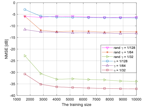
Figure 2: The normalized mean square error vs. the training size $N$.

Next, we show the impact of the training size $N$ on the reconstruction performance, as shown in Fig. 2. For a certain compression ratio, the NMSE gradually decreases and eventually tends to converge as the value $N$ increases, indicating that greater reconstruction performance may be obtained with a larger training size. Moreover, the computational complexity of Algorithm 1 is proportional to $N$, which determines the time required to learn the dictionaries. Based on this phenomenon, it is possible to make a trade-off between the reconstruction performance and the training time. Meanwhile, we also show the cases of randomly selected landmarks, which performs worse than our proposed MLCF method.

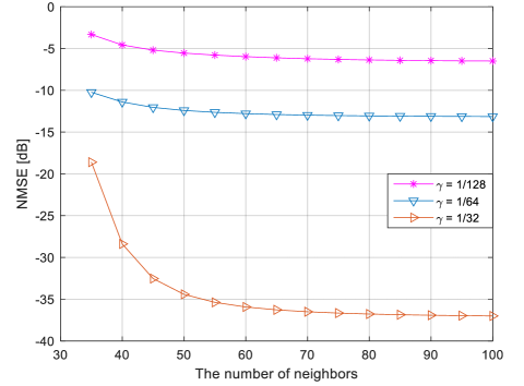
Figure 3: The normalized mean square error vs. the number of neighbors $k$.

We now investigate how the number of nearest neighbors $k$ affects the reconstruction quality. Fig. 3 depicts the relationship between the NMSE and $k$, with each curve representing a compression ratio. The value $k$ ranges from 35 to 100 with a step size of 5. It can be found that as $k$ increases, the NMSE decreases, indicating that having more neighbors enhances the reconstruction performance.

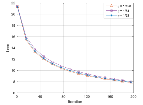
Figure 4: The loss of the objective function Eq. (18) vs. the number of iterations.

Since the explicit mapping function $f$ is not available, the problem of dimensionality reduction is solved by optimizing the objective function Eq. (18), which is the upper bound of the original objective function Eq. (16). In this simulation, we verify the convergence of Algorithm 1, as shown in Fig. 4. In each iteration, the updated dictionary and weight matrix are used to calculate the loss value of Eq. (18). The loss value is affected by the training size $N$, thus it is divided by $N$ for normalization. We discover that the loss of Eq. (18) ultimately converges after numerous iterations, which is aligned with our theoretical analysis in Theorem 3.

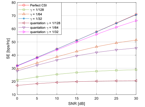
Figure 5: The spectral efficiency vs. SNR, $\lambda=0.001$, 8 UEs.

Finally, Fig. 5 shows the spectral efficiency of FDD massive MIMO systems with different signal-to-noise ratios (SNRs). The downlink precoder is Zero-Forcing. The curve labeled “Perfect CSI” means the BS has perfect downlink CSI, which is the upper-bound. In the meantime, quantization is taken into account in the CSI feedback process. The low-dimensional embeddings are quantized by 8 bits at the UEs before being transmitted to the BS. When the compression ratio $\gamma$ is 1/32, the SE performance is very close to the ideal case, indicating that the error between the reconstructed channel and the original channel is very small. However, with lower compression ratios and quantization, a degradation in performance is observed, which is expected.

VI Conclusion

In this paper, we proposed a novel manifold learning-based CSI feedback framework to reduce the feedback overhead of FDD massive MIMO systems. With no prior knowledge of the manifold where the CSI resides, we constructed a data set consisting of high-density CSI samples. Considering the local geometry on the manifold, a landmark selection algorithm was proposed to learn the most representative landmarks on the manifold so as to reconstruct all samples in the data set with minimal error. At the same time, the convergence of the algorithm was proved theoretically. Based on the pre-obtained landmarks, we proposed a low-complexity algorithm to efficiently compress and reconstruct the incremental CSI by keeping the local relationships with the landmarks unchanged. Simulation results showed that our proposed MLCF retained the advantages of manifold learning to achieve dimensionality reduction, and had superior reconstruction performance than existing CS- and DL-based algorithms.

Appendix A Proof of Proposition 1

Proof : For an arbitrary CSI sample ${{\boldsymbol{x}}_{i}}=g({{\boldsymbol{y}}_{i}})$, the linear structure of its neighborhood can be characterized by the tangent space of the manifold $\mathcal{M}$ at ${{\boldsymbol{x}}_{i}}$. Assume the manifold is smooth enough and the dictionaries have been obtained. Using first-order Taylor expansion of $g$ at ${{\boldsymbol{x}}_{i}}$, a neighbor ${{\boldsymbol{d}}_{j}}=g({{\boldsymbol{c}}_{j}})$ in the landmarks can be represented as

$${{\boldsymbol{d}}_{j}}={{\boldsymbol{x}}_{i}}+{\boldsymbol{J}_{g}}({{\boldsymbol{y}}_{i}})({{\boldsymbol{c}}_{j}}-{{\boldsymbol{y}}_{i}})+{\boldsymbol{\delta}}({{\boldsymbol{y}}_{i}},{{\boldsymbol{c}}_{j}}),$$ (42)

where ${\boldsymbol{J}_{g}}({{\boldsymbol{y}}_{i}})\in{\mathbb{R}^{2N_{f}\times d}}$ is the Jacobi matrix of $g$ at ${{\boldsymbol{y}}_{i}}$, whose column vectors span the tangent space, and ${\boldsymbol{\delta}}({{\boldsymbol{y}}_{i}},{{\boldsymbol{c}}_{j}})$ is the reminder term beyond the first-order expansion, which measures the approximation error of ${{\boldsymbol{x}}_{i}}$ to the tangent space. In particular, the $l$-th component of ${\boldsymbol{\delta}}({{\boldsymbol{y}}_{i}},{{\boldsymbol{c}}_{j}})$ is approximately equal to ${\delta}_{l}\approx\frac{1}{2}{({{\boldsymbol{c}}_{j}}-{{\boldsymbol{y}}_{i}})^{T}}{\boldsymbol{\Psi}_{g_{l}}}({y_{i}})({{\boldsymbol{c}}_{j}}-{{\boldsymbol{y}}_{i}})$, where ${\boldsymbol{\Psi}_{g_{l}}}({{\boldsymbol{y}}_{i}})$ is the Hessian matrix of the $l$-th component function $g_{l}$ of $g$ at ${{\boldsymbol{y}}_{i}}$.

Based on the sum-to-one constraint $\sum\nolimits_{j=1}^{M}{{w_{ji}}}=1$, the error between the sample ${\boldsymbol{x}_{i}}$ and its local linear approximation is

$$\begin{aligned} {\varepsilon_{i}}=\left\|{{\boldsymbol{x}_{i}}-\sum\limits_{j=1}^{M}{{w_{ji}}{\boldsymbol{d}_{j}}}}\right\|=\left\|{\sum\limits_{j=1}^{M}{w_{ji}\left({{\boldsymbol{x}}_{i}}-{{\boldsymbol{d}}_{j}}\right)}}\right\|\end{aligned}.$$ (43)

Substituting Eq. (42) into the above error, we have

$${\varepsilon_{i}} =\left\|{\sum\limits_{j=1}^{M}{w_{ji}}\left({{\boldsymbol{J}_{g}}({{\boldsymbol{y}}_{i}})({{\boldsymbol{c}}_{i}}-{{\boldsymbol{y}}_{j}})+{\boldsymbol{\delta}}({{\boldsymbol{y}}_{i}},{{\boldsymbol{c}}_{j}})}\right)}\right\|$$ (44)

$$\leq\left\|{{\boldsymbol{J}_{g}}({{\boldsymbol{y}}_{i}})\sum\limits_{j=1}^{M}{{w_{ji}}({{\boldsymbol{c}}_{i}}-{{\boldsymbol{y}}_{j}})}}\right\|+\xi\sum\limits_{j=1}^{M}\left\|{{\boldsymbol{\delta}}({{\boldsymbol{y}}_{i}},{{\boldsymbol{c}}_{j}})}\right\|$$

$$\leq\left\|{{\boldsymbol{J}_{g}}({{\boldsymbol{y}}_{i}})\sum\limits_{j=1}^{M}{{w_{ji}}({{\boldsymbol{c}}_{i}}-{{\boldsymbol{y}}_{j}})}}\right\|$$

$$\ \ \ \ \ \ \ \ \ \ \ \ +\xi\sum\limits_{j=1}^{M}\sum\limits_{l=1}^{2N_{f}}\left\|{{\frac{1}{2}{({{\boldsymbol{c}}_{i}}-{\boldsymbol{y}_{j}})}^{T}{\boldsymbol{\Psi}}_{g_{l}}({\boldsymbol{y}_{i}})({{\boldsymbol{c}}_{i}}-{{\boldsymbol{y}}_{j}})}}\right\|$$

$$\leq\underbrace{\left\|{{\boldsymbol{J}_{g}}({{\boldsymbol{y}}_{i}})(\sum\limits_{j=1}^{M}{w_{ji}}{{\boldsymbol{c}}_{j}}-{{\boldsymbol{y}}_{i}})}\right\|}_{e_{1}}+\underbrace{{\xi_{1}}\left\|{\boldsymbol{\Psi}}\right\|_{F}\sum\limits_{j=1}^{M}{{\left\|{{\boldsymbol{c}}_{i}}-{{\boldsymbol{y}}_{j}}\right\|}^{2}}}_{e_{2}},$$

where $\xi=\max{\{{w_{ji}}\}}_{j}$ is the largest entry in ${{\boldsymbol{w}}_{i}}$, $\xi_{1}=\sqrt{\frac{N_{f}}{2}}\xi$, and ${\boldsymbol{\Psi}}=\left[{\begin{array}[]{*{20}{c}}{\boldsymbol{\Psi}^{T}_{g_{1}}}({{\boldsymbol{y}}_{i}})&\cdots&{\boldsymbol{\Psi}^{T}_{g_{2N_{f}}}}({{\boldsymbol{y}}_{i}})\end{array}}\right]^{T}\in{\mathbb{R}^{2N_{f}d\times d}}$.

Two terms make up the approximation error, as can be seen. In the first term, since the column vectors of ${\boldsymbol{J}_{g}}({{\boldsymbol{y}}_{i}})$ span the tangent space of $g$ at ${{\boldsymbol{y}}_{i}}$, ${\boldsymbol{J}_{g}}({{\boldsymbol{y}}_{i}}){{\boldsymbol{y}}_{i}}$ represents the projection of ${{\boldsymbol{y}}_{i}}$ on the tangent space. Therefore, $e_{1}$ reflects the projected distance between ${{\boldsymbol{y}}_{i}}$ and $\sum\nolimits_{j}{{w_{ji}}{{\boldsymbol{c}}_{j}}}$ on the tangent space. In the second term, the Hessian matrix ${\boldsymbol{\Psi}}$ and its upper bound ${\left\|{\boldsymbol{\Psi}}\right\|_{F}}$ are determined by the local curvature of the manifold at ${{\boldsymbol{x}}_{i}}$. We have no prior knowledge of the manifold structure in a learning task, hence the constrains on the manifold are impractical in real implementations. Taking another shortcut, we consider the influence of neighbors on the approximation error. The error of the first term can be rewritten as

$${e_{1}}\leq\xi\left\|{\boldsymbol{J}_{g}}({{\boldsymbol{y}}_{i}})\right\|_{F}\sum\limits_{j=1}^{M}\left\|{\boldsymbol{c}_{j}}-{\boldsymbol{y}_{i}}\right\|.$$ (45)

If the neighbors of ${{\boldsymbol{x}}_{i}}$ in the dictionary lie in a sufficiently compact region, the hyperplane spanned by the neighbors is almost the same as the tangent space. In this case, $\max{\{\left\|{\boldsymbol{c}_{j}}-{\boldsymbol{y}_{i}}\right\|\}}_{j}$ will be tiny. Meanwhile, ${\left\|{\boldsymbol{\Psi}}\right\|}_{F}$ will be zero or close to zero. At this point, the approximation error ${\varepsilon_{i}}$ is undoubtedly quite small. Thus, Proposition 1 is proved. $\square$

Appendix B Proof of Theorem 1

Proof : Eliminating the terms irrelevant to ${\boldsymbol{d}}_{j}$, Eq. (21) can be simplified to

$$\begin{aligned} \mathcal{L}({\boldsymbol{d}}_{j})&=\|{{\boldsymbol{E}}-{{\boldsymbol{d}}_{j}}{{\boldsymbol{W}}_{j*}}}\|_{F}^{2}+\lambda\sum\limits_{i=1}^{N}{w_{ji}^{2}{{\|{{{\boldsymbol{x}}_{i}}-{{\boldsymbol{d}}_{j}}}\|}^{2}}}\\ &={\rm{tr}}\left\{({\boldsymbol{E}}-{{\boldsymbol{d}}_{j}}{{\boldsymbol{W}}_{j*}})({\boldsymbol{E}}-{{\boldsymbol{d}}_{j}}{{\boldsymbol{W}}_{j*}})^{T}\right\}\\ &\ \ \ \ \ \ \ \ \ \ \ +\lambda\sum\limits_{i=1}^{N}{w_{ji}^{2}({{\boldsymbol{x}}_{i}}-{{\boldsymbol{d}}_{j}})^{T}({{\boldsymbol{x}}_{i}}-{{\boldsymbol{d}}_{j}})}\end{aligned},$$ (46)

where each term employs the $L_{p}$-norm regularizer and satisfies $p\geq 1$. Obviously, the objective function Eq. (46) is convex.

The gradient of $\mathcal{L}({\boldsymbol{d}}_{j})$ with regard to ${{\boldsymbol{d}}_{j}}$ is

$$\frac{\partial\mathcal{L}({\boldsymbol{d}}_{j})}{\partial{\boldsymbol{d}}_{j}}=-2({\boldsymbol{E}}-{{\boldsymbol{d}}_{j}}{{\boldsymbol{W}}_{j*}}){{\boldsymbol{W}}_{j*}^{T}}-2\lambda\sum\limits_{i=1}^{N}{w_{ji}^{2}}({{\boldsymbol{x}}_{i}}-{{\boldsymbol{d}}_{j}}).$$ (47)

By setting ${{\partial\mathcal{L}({\boldsymbol{d}}_{j})}\mathord{\left/{\vphantom{{\partial\mathcal{L}({\boldsymbol{d}}_{j})}{\partial{\boldsymbol{d}_{j}}}}}\right.\kern-1.2pt}{\partial{\boldsymbol{d}}_{j}}}$ to be zero, the optimal solution to ${\boldsymbol{d}_{j}}$ is as follows

$${{\boldsymbol{d}}_{j}}=\frac{{\boldsymbol{E}}{\boldsymbol{W}}_{j*}^{T}+\lambda{\boldsymbol{X}}{({\boldsymbol{W}_{j*}^{2})}^{T}}}{(1+\lambda){{{\boldsymbol{W}}_{j*}}{{\boldsymbol{W}}}_{j*}^{T}}},$$ (48)

where ${\boldsymbol{W}}_{j*}^{2}$ represents the square of each entry in ${\boldsymbol{W}}_{j*}$, and ${\boldsymbol{X}}{({\boldsymbol{W}_{j*}^{2}})}^{T}=\sum\limits_{i=1}^{N}w_{ji}^{2}{{\boldsymbol{x}}_{i}}$. Thus, Theorem 1 is proved. $\square$

Appendix C Proof of Theorem 2

Proof : Taking the constraint ${\boldsymbol{e}}^{T}{\hat{\boldsymbol{w}}_{i}}=1$ into account, the first term in Eq. (23) can be rewritten as

$${\left\|{{\boldsymbol{x}}_{i}}-{\boldsymbol{N}}_{{\boldsymbol{x}}_{i}}{{\hat{\boldsymbol{w}}}_{i}}\right\|^{2}}={\left\|({\boldsymbol{x}_{i}}{\boldsymbol{e}}^{T}-{\boldsymbol{N}}_{{\boldsymbol{x}}_{i}}){\hat{\boldsymbol{w}}_{i}}\right\|^{2}}={{\hat{\boldsymbol{w}}}_{i}^{T}}{\boldsymbol{R}}{{\hat{\boldsymbol{w}}}_{i}},$$ (49)

where ${\boldsymbol{R}}=({\boldsymbol{x}_{i}}{\boldsymbol{e}}^{T}-{\boldsymbol{N}}_{{\boldsymbol{x}}_{i}})^{T}({\boldsymbol{x}_{i}}{\boldsymbol{e}}^{T}-{\boldsymbol{N}}_{{\boldsymbol{x}}_{i}})$.

The second term can be reformulated as

$$\sum\limits_{j=1}^{k}{\hat{w}_{ji}^{2}{{\|{\boldsymbol{x}_{i}}-{\boldsymbol{d}_{a_{j}}}\|}^{2}}}={{\hat{\boldsymbol{w}}}_{i}^{T}}\varphi({\boldsymbol{R}}){{\hat{\boldsymbol{w}}}_{i}}.$$ (50)

Note that ${\|{\boldsymbol{x}_{i}}-{\boldsymbol{d}_{a_{1}}}\|}^{2},\cdots,{\|{\boldsymbol{x}_{i}}-{\boldsymbol{d}_{a_{k}}}\|}^{2}$ are the same as the diagonal elements of ${\boldsymbol{R}}$. We define a matrix operator $\varphi(\cdot)$ that preserves only the diagonal elements of the matrix and sets the rest to zero. Therefore, for simplicity, we have $\varphi({\boldsymbol{R}})={\rm{diag}}({{\|{\boldsymbol{x}_{i}}-{\boldsymbol{d}_{a_{1}}}\|}^{2}},\cdots,{{\|{\boldsymbol{x}_{i}}-{\boldsymbol{d}_{a_{k}}}\|}^{2}})$.

The derivative of the third term ${\left\|{\boldsymbol{W}}\right\|_{2,1}}$ equals the derivative of ${\rm{tr}}({\boldsymbol{W}}^{T}{\boldsymbol{G}}{\boldsymbol{W}})$, which has been defined in Eq. (24).

The above three items all satisfy the norm greater than or equal to 1, thus it is clear that Eq. (23) is a convex function. Introducing the Lagrange multiplier, the optimization problem can be reformulated as

$$\begin{aligned} \mathcal{L}({{\hat{\boldsymbol{w}}}_{i}},\eta)&={\left\|{{\boldsymbol{x}}_{i}}-{\boldsymbol{N}}_{{\boldsymbol{x}}_{i}}{{\hat{\boldsymbol{w}}}_{i}}\right\|^{2}}+\lambda\sum\limits_{j=1}^{k}{\hat{w}_{ji}^{2}{{\|{\boldsymbol{x}_{i}}-{\boldsymbol{d}_{a_{j}}}\|}^{2}}}\\ &\ \ \ +\mu{\rm{tr}}({\boldsymbol{W}}^{T}{\boldsymbol{G}}{\boldsymbol{W}})+\eta({\boldsymbol{e}}^{T}{{\hat{\boldsymbol{w}}}_{i}}-1)\\ &={{\hat{\boldsymbol{w}}}_{i}^{T}}\left({\boldsymbol{R}}+\lambda\varphi(\boldsymbol{R})\right){{\hat{\boldsymbol{w}}}_{i}}+\mu{\rm{tr}}({\boldsymbol{W}}^{T}{\boldsymbol{G}}{\boldsymbol{W}})\\ &\ \ \ +\eta({\boldsymbol{e}}^{T}{{\hat{\boldsymbol{w}}}_{i}}-1)\end{aligned}.$$ (51)

Setting the partial derivatives of $\mathcal{L}({{\hat{\boldsymbol{w}}}_{i}},\eta)$ with regard to ${{\hat{\boldsymbol{w}}}_{i}}$ and $\eta$ to be zero, we have

$$\left\{{\begin{aligned} &{\frac{{\partial{\cal\mathcal{L}}}}{{\partial{{\hat{\boldsymbol{w}}}_{i}}}}=2\left({\boldsymbol{R}}+\lambda\varphi({\boldsymbol{R}})\right){{\hat{\boldsymbol{w}}}_{i}}+2\mu{\hat{\boldsymbol{G}}}{{\hat{\boldsymbol{w}}}_{i}}+\eta{\boldsymbol{e}}=0}\\ &\ {\frac{{\partial{\cal\mathcal{L}}}}{{\partial\eta}}={{\boldsymbol{e}}^{T}}{{\hat{\boldsymbol{w}}}_{i}}-1=0}\end{aligned}}\right.,$$ (52)

where ${\hat{\boldsymbol{G}}}={\rm{diag}}(g_{a_{1}a_{1}},g_{a_{2}a_{2}},\cdots,g_{a_{k}a_{k}})\in{\mathbb{R}^{k\times k}}$. Therefore, we have the optimal solution to the weight sub-vector as

$${\hat{\boldsymbol{w}}_{i}}=\frac{{{\left({\boldsymbol{R}}+\lambda\varphi({\boldsymbol{R}})+\mu{\hat{\boldsymbol{G}}}\right)}^{-1}}{\boldsymbol{e}}}{{\boldsymbol{e}^{T}}{\left({\boldsymbol{R}}+\lambda\varphi({\boldsymbol{R}})+\mu{\hat{\boldsymbol{G}}}\right)^{-1}}{\boldsymbol{e}}}.$$ (53)

Thus, Theorem 2 is proved. $\square$

References

- [1] Y. Cao, H. Yin, G. He, and M. Debbah, “Manifold Learning-Based CSI Feedback in Massive MIMO Systems,” in IEEE International Conference on Communications (IEEE ICC 2022), Seoul,South Korea, May 2022, pp. 225–230.
- [2] E. G. Larsson, O. Edfors, F. Tufvesson, and T. L. Marzetta, “Massive MIMO for next generation wireless systems,” IEEE Commun. Mag., vol. 52, no. 2, pp. 186–195, Feb. 2014.
- [3] T. L. Marzetta, “Massive MIMO: an introduction,” Bell Labs Tech. J., vol. 20, pp. 11–22, 2015.
- [4] ——, “Noncooperative cellular wireless with unlimited numbers of base station antennas,” IEEE Trans. Wireless Commun., vol. 9, no. 11, pp. 3590–3600, Nov. 2010.
- [5] D. J. Love, R. W. Heath, V. K. Lau, D. Gesbert, B. D. Rao, and M. Andrews, “An overview of limited feedback in wireless communication systems,” IEEE J. Sel. Areas Commun., vol. 26, no. 8, pp. 1341–1365, 2008.
- [6] Z. Qin, H. Yin, Y. Cao, W. Li, and D. Gesbert, “A partial reciprocity-based channel prediction framework for FDD massive MIMO with high mobility,” IEEE Transactions on Wireless Communications, vol. 21, no. 11, pp. 9638–9652, 2022.
- [7] P. Liang, J. Fan, W. Shen, Z. Qin, and G. Y. Li, “Deep learning and compressive sensing-based CSI feedback in FDD massive MIMO systems,” IEEE Trans. Veh. Technol., vol. 69, no. 8, pp. 9217–9222, Aug. 2020.
- [8] V. Raghavan, R. W. Heath, and A. M. Sayeed, “Systematic codebook designs for quantized beamforming in correlated MIMO channels,” IEEE J. Sel. Areas Commun., vol. 25, no. 7, pp. 1298–1310, Sep. 2007.
- [9] K. Kim, T. Kim, D. J. Love, and I. H. Kim, “Differential feedback in codebook-based multiuser MIMO systems in slowly varying channels,” IEEE Trans. Commun., vol. 60, no. 2, pp. 578–588, 2012.
- [10] P.-H. Kuo, H. Kung, and P.-A. Ting, “Compressive sensing based channel feedback protocols for spatially-correlated massive antenna arrays,” in 2012 IEEE Wireless Communications and Networking Conference (WCNC), Apr. 2012, pp. 492–497.
- [11] Z. Gao, L. Dai, S. Han, I. Chih-Lin, Z. Wang, and L. Hanzo, “Compressive sensing techniques for next-generation wireless communications,” IEEE Wireless Commun., vol. 25, no. 3, pp. 144–153, 2018.
- [12] P. N. Alevizos, X. Fu, N. D. Sidiropoulos, Y. Yang, and A. Bletsas, “Limited feedback channel estimation in massive MIMO with non-uniform directional dictionaries,” IEEE Trans. Signal Process., vol. 66, no. 19, pp. 5127–5141, 2018.
- [13] H. Sun, Z. Zhao, X. Fu, and M. Hong, “Limited feedback double directional massive MIMO channel estimation: From low-rank modeling to deep learning,” in 2018 IEEE 19th International Workshop on Signal Processing Advances in Wireless Communications (SPAWC), 2018, pp. 1–5.
- [14] C. Tian, A. Liu, M. B. Khalilsarai, G. Caire, W. Luo, and M.-J. Zhao, “Randomized channel sparsifying hybrid precoding for FDD massive MIMO systems,” IEEE Trans. Wireless Commun., vol. 19, no. 8, pp. 5447–5460, 2020.
- [15] Y. Yang, F. Gao, G. Y. Li, and M. Jian, “Deep learning-based downlink channel prediction for FDD massive MIMO system,” IEEE Commun. Lett., vol. 23, no. 11, pp. 1994–1998, 2019.
- [16] C.-K. Wen, W.-T. Shih, and S. Jin, “Deep learning for massive MIMO CSI feedback,” IEEE Wireless Commun. Lett., vol. 7, no. 5, pp. 748–751, Oct. 2018.
- [17] Z. Lu, J. Wang, and J. Song, “Multi-resolution CSI feedback with deep learning in massive MIMO system,” in ICC 2020-2020 IEEE International Conference on Communications (ICC), June 2020, pp. 1–6.
- [18] T. Wang, C.-K. Wen, S. Jin, and G. Y. Li, “Deep learning-based CSI feedback approach for time-varying massive MIMO channels,” IEEE Wireless Communications Letters, vol. 8, no. 2, pp. 416–419, 2018.
- [19] Z. Cao, W.-T. Shih, J. Guo, C.-K. Wen, and S. Jin, “Lightweight convolutional neural networks for CSI feedback in massive MIMO,” IEEE Commun. Lett., vol. 25, no. 8, pp. 2624–2628, Aug. 2021.
- [20] T. Lin and H. Zha, “Riemannian manifold learning,” IEEE Trans. Pattern Anal. Mach. Intell., vol. 30, no. 5, pp. 796–809, May 2008.
- [21] S. T. Roweis and L. K. Saul, “Nonlinear dimensionality reduction by locally linear embedding,” Science, vol. 290, no. 5500, pp. 2323–2326, 2000.
- [22] Z. Zhang and H. Zha, “Principal manifolds and nonlinear dimensionality reduction via tangent space alignment,” SIAM J. Sci. Comput., vol. 26, no. 1, pp. 313–338, 2004.
- [23] W. Li, H. Yin, Z. Qin, Y. Cao, and M. Debbah, “A Multi-Dimensional Matrix Pencil-Based Channel Prediction Method for Massive MIMO with Mobility,” IEEE Transactions on Wireless Communications, 2022.
- [24] H. Yin, D. Gesbert, M. Filippou, and Y. Liu, “A coordinated approach to channel estimation in large-scale multiple-antenna systems,” IEEE J. Sel. Areas Commun., vol. 31, no. 2, pp. 264–273, 2013.
- [25] A. Adhikary, J. Nam, J.-Y. Ahn, and G. Caire, “Joint spatial division and multiplexing—The large-scale array regime,” IEEE Trans. Inf. Theory, vol. 59, no. 10, pp. 6441–6463, 2013.
- [26] H. Yin, D. Gesbert, and L. Cottatellucci, “Dealing with interference in distributed large-scale MIMO systems: A statistical approach,” IEEE J. Sel. Top. Signal Process., vol. 8, no. 5, pp. 942–953, 2014.
- [27] C. Zhang, J. Wang, N. Zhao, and D. Zhang, “Reconstruction and analysis of multi-pose face images based on nonlinear dimensionality reduction,” Pattern Recognition, vol. 37, no. 2, pp. 325–336, 2004.
- [28] 3GPP, Study on channel model for frequencies from 0.5 to 100 GHz (Release 16). Technical Report TR 38.901, available: http://www.3gpp.org, 2019.
- [29] H. Yin, H. Wang, Y. Liu, and D. Gesbert, “Addressing the curse of mobility in massive MIMO with prony-based angular-delay domain channel predictions,” IEEE J. Sel. Areas Commun., vol. 38, no. 12, pp. 2903–2917, 2020.
- [30] K. Zhang and J. T. Kwok, “Clustered Nyström method for large scale manifold learning and dimension reduction,” IEEE Trans. Neural Networks, vol. 21, no. 10, pp. 1576–1587, 2010.
- [31] W. M. Boothby and W. M. Boothby, An introduction to differentiable manifolds and Riemannian geometry. Gulf Professional Publishing, 2003, vol. 120.
- [32] S. K. Sahoo and A. Makur, “Dictionary training for sparse representation as generalization of k-means clustering,” IEEE Signal Process Lett., vol. 20, no. 6, pp. 587–590, 2013.
- [33] F. Nie, H. Huang, X. Cai, and C. Ding, “Efficient and robust feature selection via joint L2,1-norms minimization,” Advances in neural information processing systems, vol. 23, 2010.
- [34] S. Boyd, S. P. Boyd, and L. Vandenberghe, Convex optimization. Cambridge university press, 2004.
- [35] C. Li, W. Yin, and Y. Zhang, “User’s guide for TVAL3: TV minimization by augmented lagrangian and alternating direction algorithms,” CAAM report, vol. 20, no. 46-47, p. 4, 2009.
- [36] I. Daubechies, M. Defrise, and C. De Mol, “An iterative thresholding algorithm for linear inverse problems with a sparsity constraint,” Commun. Pure Appl. Math., vol. 57, no. 11, pp. 1413–1457, Nov. 2004.