Smooth Indirect Solution Method for State-constrained Optimal Control Problems with Nonlinear Control-affine Systems

Abstract

This paper proposes a new indirect solution method for solving state-constrained optimal control problems by revisiting the well-established optimal control theory and addressing the long-standing issue of discontinuous control and costate due to pure state inequality constraints. It is well-known that imposing pure state path constraints in optimal control problems introduces discontinuities in the control and costate, rendering the classical indirect solution methods ineffective to numerically solve state-constrained problems. This study re-examines the necessary conditions of optimality for a class of state-constrained optimal control problems, and shows the uniqueness of the optimal control input that minimizes the Hamiltonian on constrained arcs. This analysis leads to a unifying form of optimality necessary conditions and thereby address the issue of discontinuities in control and costate by modeling them via smooth functions, transforming the originally discontinuous problems to smooth two-point boundary value problems (TPBVPs), which can be readily solved by existing nonlinear root-finding algorithms. The proposed solution method is shown to have favorable properties, including its anytime algorithm-like property, which is often a desirable property for safety-critical applications, and numerically demonstrated by an optimal orbital transfer problem.

I Introduction

This paper proposes a new indirect solution method for solving state-constrained optimal control problems by revisiting the well-established optimal control theory and addressing the long-standing issue of discontinuous costate and control due to state constraints. It is well-known that imposing pure state path constraints (i.e., constraints in the form $S(x,t)\leq 0$) in optimal control problems introduces discontinuities in the control and costate when the trajectory enters constrained arcs [1, 2, 3]. Despite such difficulties, state-constrained optimal control problems arise in many fields, including aerospace, robotics, and other engineering and applied science applications.

In practice, many state-constrained optimal control problems are currently solved by using direct methods. Direct methods are a class of solution methods that convert continuous-time optimal control problems into finite-dimensional problems by parameterizing the problems via multiple shooting [4], numerical collocation [5], or exact time discretization [6]. The resulting parameter optimization problems are solved via nonlinear programming [7], sequential convex programming [8], model predictive control [9], etc. Many successful commercial software for solving general optimal control problems, such as GPOPS [10], fall under the category of direct methods. To incorporate inequality constraints in the direct method framework, they almost always employ the penalty function method and its variants [11, 12, 13], which impose “soft” constraints by penalizing the violation of constraints and increase the penalty weight over iterations, asymptotically achieving the feasibility starting from infeasible solutions (note that those using exact penalty functions may not require iterations on the penalty weight as long as “sufficiently large” penalty weight is initially chosen [14]). These methods are often combined with techniques in numerical optimization, such as the interior point method [7] and the augmented Lagrangian method [15, 16].

Although direct methods provide flexibility in solving large-scale problems, they often compromise the feasibility and/or optimality of the solution, mainly due to the problem parameterization and the approximate equations of motion. The computational complexity can be also an issue due to the large number of variables (usually a few hundreds to a few thousands) introduced by the parameterization when the computational resources are limited. Furthermore, since most direct methods are based on the penalty function methods, the feasibility is not necessarily guaranteed if the solver is prematurely terminated [17, 11]. In contrast, indirect methods possess a remarkable advantage due to the fewer dimensionality of the problem (less than 10 unknowns for three-dimensional optimal control problems). The fewer dimensionality is highly attractive particularly when the control problem is complex, involving covariance control [18, 19] and/or multiple phases [20].

Motivated by these observations, the objective of this paper is to revisit the use of indirect methods, the classical solution methods for optimal control problems based on the direct application of Pontryagin’s minimum principle [2, 21], and develop a computationally efficient indirect solution method for state-constrained problems. Classical indirect methods for state-constrained problems divide the entire trajectory into sub-arcs and solve each sub-arc as separate two-point boundary value problems (TPBVPs) while satisfying the transversality conditions [1, 2, 3]. This approach, however, is ineffective to numerically solve the problems due to its major drawbacks, namely, (1) it has to deal with discontinuities in control and costate; and (2) it requires a priori information about the structure of sub-arcs (e.g., number of constrained arcs). These drawbacks virtually limit the application of the classical approach to analytic examples (e.g., Examples 1 and 2 in Ref. [2] and the examples in Refs. [1, 22]). Obviously, many meaningful problems in practice tends to be complex, and it is rare that these problems can be analytically solved, requiring improved numerical solution methods.

Therefore, this study proposes a solution method that efficiently solves complex state-constrained optimal control problems via indirect methods. First, this paper re-examines the necessary conditions of optimality for state-constrained optimal control problems with a nonlinear control-affine system, which arises in many aerospace [23, 24] and robotic systems [25, 26]; we then show the uniqueness of the optimal control input that minimizes the Hamiltonian on constrained arcs. This analysis leads to a unifying form of optimality necessary conditions, enabling us to address the issue of discontinuities in control and costate by modeling them via smooth (i.e., continuously differentiable) functions. With this approach, the originally discontinuous problems are transformed to smooth TPBVPs with sharpness parameters $\rho$, which can be readily solved by existing nonlinear root-finding algorithms. The optimality of the solution is controlled by $\rho$, where the solution approaches the optimum as $\rho$ approaches zeros, allowing a continuation over $\rho$ to obtain a sequence of improving solutions. Moreover, it is shown that each intermediate solution in the continuation process respects the state constraint $S(\cdot)\leq 0$, which is often a desirable property when considering the application to safety-critical systems.

II Preliminary

II-A Problem Statement

Consider a nonlinear, control-affine dynamical system:

$$\dot{x}=f(x,u,t)=f_{0}(x,t)+\sum_{i=1}^{m}f_{i}(x,t)u_{i},$$ (1)

where $x\in\mathbb{R}^{n}$, $u\in\mathbb{R}^{m}$, and $t\in\mathbb{R}$ denote the system state, control, and time, respectively. It is assumed that $f_{i}(\cdot),\ i=0,1,...,m$ is at least twice continuously differentiable. Note that many robotic and aerospace systems with controls can be expressed as a control-affine system [24, 27, 25]. We introduce a matrix $F\in\mathbb{R}^{n\times m}$ whose columns consist of $f_{i}(\cdot),\ i=1,...,m$ to compactly express Eq. 1 as follows:

$$\dot{x}=f_{0}(x,t)+F(x,t)u,\quad F(\cdot)\triangleq\begin{bmatrix}f_{1}(\cdot)&...&f_{m}(\cdot)\end{bmatrix}$$ (2)

Without loss of generality, we consider minimizing the cost functional of the Lagrange form:

$$J=\int_{0}^{T}L(x,u,t)\mathrm{d}t.$$ (3)

A feasible trajectory must satisfy terminal constraints

$$\psi(x(0),x(T),T)=0$$ (4)

where $\psi:\mathbb{R}^{n}\times\mathbb{R}^{n}\times\mathbb{R}\mapsto\mathbb{R}^{q}$, and a scalar state constraint

$$S(x,t)\leq 0.$$ (5)

The constraint $S$ is assumed to be twice continuously differentiable and first order, implying that the first time derivative of $S$ contains the control term $u$ explicitly, i.e.,

$$\begin{aligned} \dot{S}=&\frac{\mathrm{d}S}{\mathrm{d}t}=S_{x}f+S_{t}\\ =&S_{x}f_{0}+S_{x}Fu+S_{t}\triangleq S^{(1)}(x,u,t).\end{aligned}$$ (6)

where $S_{x}\in\mathbb{R}^{1\times n},S_{t}\in\mathbb{R}$ are the gradients of $S$ with respect to $x$ and $t$ for compact notation, i.e., $S_{x}\triangleq\nabla_{x}S$ and $S_{t}\triangleq\nabla_{t}S$, respectively. The first-order constraint assumption is thus equivalent to $S_{x}F\neq 0,\ \forall x,t$.

Although the analysis in this study is focused on a scalar state constraint $S$ for conciseness, generalization to a vector-valued state constraint $S$ is straightforward by requiring a similar condition; namely, for $S\in\mathbb{R}^{l}$ with $l>1$, it is required that each row of $S_{x}F$ must be independent (similar to the well-known linear independence constraint qualification; LICQ) in addition to $S_{x}F\neq 0,\ \forall x,t$.

Thus, our original problem is formulated as in Problem 1.

Problem 1 (Original problem).

Find $x^{*}(t),u^{*}(t),T^{*}$ that minimize the cost Eq. 3 subject to the dynamics Eq. 2, terminal constraints Eq. 4, and pure state constraint Eq. 5.

II-B Optimality Necessary Conditions

The necessary conditions of optimality take different forms depending on whether the state path constraint is active ($S=0$) or not ($S<0$). Following the naming convention in [2], we call an interval of a trajectory with $S=0$ a constrained arc while that with $S<0$ an unconstrained arc. An instant $t_{i}\in[0,T]$ is called an entry time if an unconstrained arc ends at $t=t_{i}$ and a constrained arc starts at $t=t_{i}$. Likewise, $t_{i+1}$ is called an exit time if a constrained arc ends and an unconstrained arc starts at $t=t_{i+1}$.

To avoid confusion, this paper distinguishes the optimal controls on unconstrained arcs and constrained arcs by $u_{o}^{*}$ and $u_{c}^{*}$, respectively. $u^{*}$ with no subscript collectively represents the optimal control regardless of the arcs the trajectory is currently on.

Clearly, a trajectory is characterized as follows:

$$\begin{aligned} \begin{cases}\mathrm{unconstrained\ arc}&\mathrm{if\ }S<0\\ \mathrm{constrained\ arc}&\mathrm{if\ }S=0\ \land\ S^{(1)}_{o}\geq 0\\ \mathrm{infeasible}&\mathrm{if\ }S>0\end{cases}\end{aligned}$$ (7)

where $S^{(1)}_{o}$ is a shorthand notation of $S^{(1)}(\cdot)$ under $u_{o}^{*}$, i.e., $S^{(1)}_{o}\triangleq S^{(1)}(x,u_{o}^{*},t)$. When $S=0$ and $S^{(1)}_{o}\leq 0$ at $t=t_{i}$, the trajectory is leaving the constrained arc, i.e., an exit point, while it is necessarily $S=0$ and $S^{(1)}_{o}>0$ at an entry point.

II-B1 Unconstrained arc

On an unconstrained arc, from Pontryagin’s optimality principle, $u_{o}^{*}$ must satisfy

$$u_{o}^{*}\in\arg\min_{u}H_{o}$$ (8)

where $H_{o}$ represents the control Hamiltonian of the unconstrained problem. $H_{o}$ is defined as:

$$\begin{aligned} H_{o}(x,u,\lambda,t)=L(x,u,t)+\lambda^{\top}[f_{0}(x,t)+F(x,t)u]\end{aligned}$$ (9)

where $\lambda\in\mathbb{R}^{n}$ is the Lagrange multiplier associated with Eq. 2, also known as costate. The costate must satisfy the following differential equation:

$$-\dot{\lambda}^{\top}=\nabla_{x}H_{o}=\nabla_{x}L+\lambda^{\top}\nabla_{x}f$$ (10)

II-B2 Constrained arc

On a constrained arc, a feasible control must satisfy $S^{(1)}(x,u,t)\leq 0$. Among several approaches in literature [1], this study takes an approach known as indirect adjoining to derive the necessary conditions.

The indirect adjoining approach adjoins the control-dependent constraint $S^{(1)}(x,u,t)\leq 0$ in addition to Eqs. 2 and 4 to yield the control Hamiltonian [2]:

$$\begin{aligned} H_{c}(x,u,\lambda,\mu,t)=L+\lambda^{\top}f+\mu S^{(1)}\end{aligned}$$ (11)

where $H_{c}$ is the control Hamiltonian on a constrained arc; $\mu(\geq 0)\in\mathbb{R}$ is a Lagrange multiplier associated with $S^{(1)}\leq 0$. A pair of the optimal control, $u_{c}^{*}$, and the optimal multiplier, $\mu^{*}$, must simultaneously satisfy [2]

$$(u_{c}^{*},\mu^{*})\in\left\{u,\mu\geq 0\mid\min_{u,\mu}H_{c}\ \text{s.t.\ }S^{(1)}=0\right\},$$ (12)

the state dynamics satisfy Eq. 2, and the costate dynamics

$$-\dot{\lambda}^{\top}=\nabla_{x}H=\nabla_{x}L+\lambda^{\top}\nabla_{x}f+\mu\nabla_{x}S^{(1)}$$ (13)

II-B3 Additional necessary condition

Although the condition $\mu\geq 0$ on a constrained arc is widely acknowledged in literature (e.g., [2]), there is an additional condition on $\mu$. Assuming a constrained arc on $t\in[t_{i},t_{i+1}]$, such an additional condition is derived as [1, 29]:

$$\begin{aligned} \dot{\mu}(t)\leq 0,\ \forall t\in[t_{i},t_{i+1}],\quad\land\quad\mu(t_{i+1}^{-})=0,\end{aligned}$$ (14)

which imply $\mu(t)\geq 0,\ \forall t\in[t_{i},t_{i+1}]$; however, its converse is not true. [30] points out that this additional condition can be crucial when the system is not autonomous. Further, this condition implies an important property of $\mu(t)$. Noting that $\mu(t_{i}^{-})=0$ ($\because$ the trajectory is on an unconstrained arc at $t_{i}^{-}$), the conditions in Eq. 14 imply that $\mu$ has to experience a discontinuous increase at $t_{i}$, i.e., $\mu(t_{i}^{-})\neq\mu(t_{i}^{+})$.

II-B4 Discontinuity at corners

The discontinuous change in $\mu^{*}$ leads to a discontinuity in $u^{*}$, as $u^{*}$ depends on $\mu^{*}$ (recall Eq. 12). The points where such discontinuities occur are called corners. It is clear from Eq. 14 that the discontinuity occurs only at entry corners in the current formulation. At each corner (say at $t=t_{i}$), $\lambda$ and $H$ generally experience a discontinuous change [22]:

$$\begin{aligned} \lambda(t_{i}^{+})&=\lambda(t_{i}^{-})-\eta_{i}[S_{x}(t_{i})]^{\top},\\ H(t_{i}^{+})&=H(t_{i}^{-})+\eta_{i}S_{t}(t_{i}),\end{aligned}$$ (15)

while no such discontinuities need occur at the exit point. It is also shown [29] that the new multiplier $\eta_{i}$ must satisfy

$$\begin{aligned} \eta_{i}=\mu(t_{i}^{+}),\end{aligned}$$ (16)

and therefore we can replace $\eta_{i}$ in Eq. 15 by $\mu(t_{i}^{+})$.

III Uniqueness of Optimal Control and Multiplier

Although the necessary conditions of optimality state the conditions that the pair $(u^{*},\mu^{*})$ must satisfy, they do not clarify whether such $(u^{*},\mu^{*})$ is unique or not.

The uniqueness of the pair $(u^{*},\mu^{*})$ is essential for numerically solving optimal control problems via indirect methods. Numerical solutions for problems with no such uniqueness guarantee typically have to rely on direct methods (e.g., GPOPS [10]) with greater computational complexity.

III-A Optimal Control on Unconstrained Arcs

We assume that the unique solution to the Hamiltonian minimization on unconstrained arcs (i.e., solution to Eq. 8) is available in a closed form and is continuously differentiable in the following form:

$$u_{o}^{*}=g(x,\lambda,t)$$ (17)

by satisfying the sufficient condition for the minimum Hamiltonian (also known as the Legendre-Clebsch condition [2]):

$$\begin{aligned} &\nabla_{u}H_{o}=\nabla_{u}L(x,u,t)+\lambda^{\top}F=0\quad\land\\ &\nabla^{2}_{uu}H_{o}=\nabla_{uu}^{2}L(x,u,t)\succ 0\end{aligned}$$ (18)

Note that this assumption holds for many problems that are solved by indirect methods, as demonstrated in Section III-D.

III-B Optimal Control on Constrained Arcs

It can be shown that, with the assumption made in Section III-A, Problem 1 has the unique pair of $(u_{c}^{*},\mu^{*})$ $\forall t$ on constrained arcs. Lemma 1 formally states this fact.

Lemma 1.

Under the assumption that the unique solution to Eq. 8 is available in a closed form Eq. 17, the solution to Eq. 12 is uniquely determined in the following form:

$$u_{c}^{*}= g(x,\lambda+\mu S_{x}^{\top},t),$$ (19)

$$\mu^{*}= h(x,\lambda,t)\geq 0,$$ (20)

where $h$ is continuously differentiable.

Proof.

The goal is to find the unique pair of $u_{c}^{*}$ and $\mu*$ that solves the following Hamiltonian minimization:

$$(u_{c}^{*},\mu^{*})=\arg\min_{\mu\geq 0}\min_{u}H_{c} \ \text{s.t.\ }S^{(1)}=0$$ (21)

where $H_{c}$ is given by Eq. 11. Expanding $H_{c}$, we have

$$H_{c}=L+(\lambda^{\top}+\mu S_{x})(f_{0}+Fu)+\mu S_{t}.$$ (22)

The Legendre-Clebsch condition for $H_{c}$ leads to

$$\nabla_{u}H_{c}=\nabla_{u}L(x,u,t)+(\lambda^{\top}+\mu S_{x})F=0\quad\land$$ (23a)

$$\nabla^{2}_{uu}H_{c}=\nabla_{uu}^{2}L(x,u,t)\succ 0$$ (23b)

Comparing this against Eq. 18, it is clear that $u_{c}^{*}$ is given by Eq. 19. Note here that Eqs. 23a and 23b must be satisfied for any $\mu$. Thus, the partial derivative of $\nabla_{u}H_{c}$ with respect to $\mu$ must be identically zero, i.e.,

$$\begin{aligned} 0=&\nabla_{\mu}[\nabla_{u}H_{c}]=\nabla_{\mu u}^{2}L(x,u_{c}^{*},t)+S_{x}F\\ =&S_{x}\left\{\left[\nabla_{\lambda}g(x,\lambda+\mu S_{x}^{\top},t)\right]^{\top}\nabla_{uu}^{2}L(x,u_{c}^{*},t)+F\right\}\end{aligned}$$

which implies that $[\nabla_{\lambda}g(x,\lambda+\mu S_{x}^{\top},t)]^{\top}\nabla_{uu}^{2}L(x,u_{c}^{*},t)+F=0$, yielding ($\because\nabla_{uu}^{2}L(x,u_{c}^{*},t)\succ 0$, so invertible)

$$\begin{aligned} \nabla_{\lambda}g(x,\lambda+\mu S_{x}^{\top},t)=-[\nabla_{uu}^{2}L(x,u_{c}^{*},t)]^{-1}F^{\top}\end{aligned}$$ (24)

Eq. 24 becomes handy shortly.

From Eq. 21, $\mu^{*}$ must satisfy $S^{(1)}=0$ under $u_{c}^{*}$ given by Eq. 19, i.e., (recall Eq. 6)

$$S^{(1)}=S_{x}f_{0}+S_{x}Fg(x,\lambda+\mu^{*}S_{x}^{\top},t)+S_{t}=0$$ (25)

Taking the partial derivative of $S^{(1)}$ with respect to $\mu$ and using Eq. 24, we have

$$\begin{aligned} \nabla_{\mu}S^{(1)}=&S_{x}F[\nabla_{\mu}g(x,\lambda+\mu S_{x}^{\top},t)]\\ =&S_{x}F[\nabla_{\lambda}g(x,\lambda+\mu S_{x}^{\top},t)]S_{x}^{\top}\\ =&-S_{x}F[\nabla_{uu}^{2}L(x,u_{c}^{*},t)]^{-1}F^{\top}S_{x}^{\top}\end{aligned}$$ (26)

which implies $\nabla_{\mu}S^{(1)}<0$ because $[\nabla_{uu}^{2}L(x,u_{c}^{*},t)]^{-1}\succ 0$ due to Eq. 23b and $S_{x}F\neq 0$, $\forall x,t$ due to the first-order constraint assumption as discussed in Section II-A. This clarifies that $S^{(1)}$ is monotonically decreasing in $\mu$. Note also that, when $\mu=0$, we have that $g(x,\lambda+\mu S_{x}^{\top},t)=g(x,\lambda,t)=u_{o}^{*}$ and hence $S^{(1)}=S^{(1)}_{o}\geq 0$ on a constrained arc (recall Eq. 7). Therefore, $\mu^{*}$ that satisfies Eq. 25 is unique and must be non-negative, and the unique solution can be represented by a function $\mu^{*}=h(x,\lambda,t)$, i.e., Eq. 20. Finally, $h(x,\lambda,t)$ is continuously differentiable because $S(\cdot)$, $f_{i}(\cdot),\ i=0,1,...,m$, and $g(\cdot)$ are twice differentiable. ∎

III-C Unified Form of Optimality Necessary Conditions

Combining Sections III-A and III-B, it is clear that we can express the necessary conditions of optimality for Problem 1 in a unified form, given in Eq. 27, without the need to separate the discussion ($\because$ on unconstrained arcs, by substituting $\mu^{*}=0$, Eq. 27a and Eq. 27b are equivalent to Eq. 17 and Eq. 10, respectively).

$$u^{*}= g(x,\lambda+\mu^{*}S_{x}^{\top},t),$$ (27a)

$$\dot{\lambda}^{*}= -(\nabla_{x}L)^{\top}-(\nabla_{x}f)^{\top}\lambda-\mu^{*}[\nabla_{x}S^{(1)}]^{\top},$$ (27b)

$$\mu^{*}= \begin{cases}0&(\text{on unconstrained arc})\\ h(x,\lambda,t)\geq 0&(\text{on constrained arc})\end{cases}$$ (27c)

This is in sharp contrast to the classical discussion in literature (e.g., [2]), which divides a state-constrained optimal control problem into constrained and unconstrained arcs.

It is worth noting that, even with the unifying form given by Eq. 27, Problem 1 still experiences discontinuities due to the jump in $\mu^{*}$ (and hence in $\lambda^{*}$ and $H^{*}$) when the trajectory enters a constrained arc, which is addressed in Section IV.

III-D Analytical Example

Let us consider an example of the cost functional $L(\cdot)$ to demonstrate the wide applicability of the assumption made in Section III-A as well as the procedure to find the unique $u^{*}$ and $\mu^{*}$ on constrained arcs based on Lemma 1. $L(\cdot)$ considered in this example is given by:

$$L(\cdot)=c(x,t)+u^{\top}Ru+x^{\top}Pu,$$ (28)

where $R\succ 0$. With this cost functional, the assumption made in Section III-A is clearly met, as the solution to Eq. 8 can be obtained by finding $u$ that satisfies the Legendre-Clebsch condition Eq. 18, as follows:

$$u_{o}^{*}=-\frac{1}{2}R^{-1}(Px+F^{\top}\lambda)$$ (29)

which is continuously differentiable ($\because F$ is continuously differentiable). It is also straightforward to derive $u^{*}$ on constrained arcs by applying Eqs. 23a and 23b, yielding:

$$u_{c}^{*}= -\frac{1}{2}R^{-1}[Px+F^{\top}(\lambda+\mu^{*}S_{x}^{\top})]$$ (30)

which clearly takes the form given in Eq. 19 (compare Eq. 30 and Eq. 29). Substituting Eq. 30 into Eq. 25 and solving for $\mu^{*}$ yields

$$\mu^{*}= \frac{2S_{x}f_{0}+2S_{t}-S_{x}FR^{-1}(Px+F^{\top}\lambda)}{S_{x}FR^{-1}F^{\top}S_{x}^{\top}}$$ (31)

where note that $S_{x}FR^{-1}F^{\top}S_{x}^{\top}\neq 0$ because $S_{x}F\neq 0$ and $R\succ 0$. Eq. 31 is continuously differentiable because $S(\cdot)$ and $f_{i}(\cdot),\ i=0,...,m$ are twice differentiable.

IV Solution Method

This section presents the proposed solution method to address discontinuities in Problem 1 and analyzes its properties.

IV-A Smooth Approximation of Discontinuous Multiplier

Noting Eqs. 27 and 7, $\mu^{*}$ switches its value between $h\geq 0$ and $0$ triggered by the constraint activation as follows:

$$\begin{aligned} \mu^{*}=\begin{cases}h(x,\lambda,t)\geq 0&S=0\ \land\ S^{(1)}_{o}\geq 0\\ 0&\mathrm{otherwise}\end{cases}\end{aligned}$$ (32)

As clear from Eq. 32, the main challenge here is to smoothly model the discontinuous behavior of $\mu^{*}$ triggered by the two conditions $S=0$ and $S^{(1)}_{o}\geq 0$. To this end, this study proposes to model $\mu^{*}$ via $\tilde{\mu}^{*}$ with two smooth activation functions as follows:

$$\begin{aligned} \tilde{\mu}^{*}&=h(x,\lambda,t)\phi_{1}(S)\phi_{2}(S^{(1)}_{o}),\end{aligned}$$ (33)

where $\phi_{1}(\cdot)$ and $\phi_{2}(\cdot)$ aim to smoothly characterize the activation of conditions $S=0$ and $S^{(1)}_{o}\geq 0$, respectively. Clearly, in order to guarantee no violation of the constraint (i.e., guaranteed feasibility), both $\phi_{1}$ and $\phi_{2}$ must take unity when $S=0$ and $S^{(1)}_{o}\geq 0$, where note that $\phi_{2}$ must not increase (nor decrease) from unity for potentially large values of $S^{(1)}_{o}$ while such a consideration is not necessary for $\phi_{1}$ ($\because S$ does not become positive when $S^{(1)}=0$ is satisfied on a constrained arc, as shown shortly). Also, in order for the approximation to be asymptotically precise, we would like $\phi_{1}$ to be close to zero when $S\neq 0$ (which is when $S<0$ since $S\not>0$) and $\phi_{2}$ to be close to zero when $S^{(1)}_{o}<0$.

Based on these desirable properties, a hyperbolic tangent-based function (a variant of the logistic function) and a variant of the bump function are chosen for $\phi_{1}(\cdot)$ and $\phi_{2}(\cdot)$, respectively. Formally defining these activation functions,

$$\phi_{1}(x)= \frac{e^{2}+1}{2e^{2}}\left(1+\tanh{\frac{x+\rho_{1}}{\rho_{1}}}\right),$$ (34a)

$$\phi_{2}(x)= \begin{cases}1&x>0\\ \exp{\left[\frac{1}{\rho_{2}^{2}}\left(1-\frac{1}{1-x^{2}}\right)\right]}&x\in(-1,0]\\ 0&x\leq-1\\ \end{cases}$$ (34b)

where $\rho_{1}\in\mathbb{R}$ and $\rho_{2}\in\mathbb{R}$ are positive scalars that control the sharpness of the approximation; smaller $\rho_{1}$ and $\rho_{2}$ lead to sharper approximations. The logistic function and bump function are widely used in the field of computer science (e.g., machine learning); the hyperbolic tangent-based formulation also finds its applications in smooth approximation of the bang-bang optimal control for low-thrust spacecraft transfers [31].

Fig. 1 illustrates their behavior with different values of $\rho$, where $\phi_{\tanh},\phi_{\mathrm{bump}}$ represent $\phi_{1},\phi_{2}$, respectively.

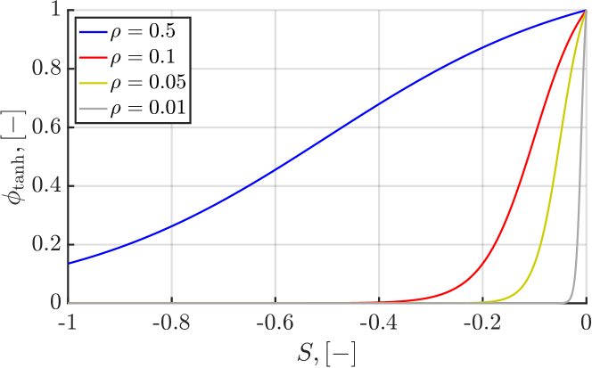
(a) Multiplier discontinuity approximation, Eq. 34a

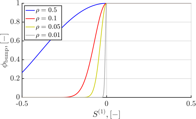
(b) Multiplier discontinuity approximation, Eq. 34b

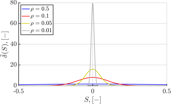
(c) Costate jump condition approximation, Eq. 38

Figure 1: Activation functions for smooth approximation with various sharpness parameters $\rho$

Lemma 2 formally states the three important properties this smooth approximation approach possesses. The first property (1) is crucial in facilitating the numerical convergence of the solution method. This property implies the smoothness of $u$ and $\dot{x}$, eliminating the need to divide the trajectory into sub-arcs. The second property (2) is vital when dealing with safety-critical systems where we do not want to compromise the feasibility of the state constraint for any $\rho$. The third property (3) ensures the convergence to the local optimum of the original problem.

Lemma 2.

The smooth approximation $\tilde{\mu}^{*}$ as defined in Eqs. 33 and 34 has the following properties:

1. $\tilde{\mu}^{*}$ is continuously differentiable over an optimal trajectory including at corners;

2. $\tilde{\mu}^{*}$ respects the inequality constraint regardless of the values of $\rho_{1}$ and $\rho_{2}$; and

3. $\tilde{\mu}^{*}$ approaches $\mu$ defined in Eq. 32 as $\rho_{1},\rho_{2}\to{+}0$.

Proof.

(1) is shown first. It is clear from Eq. 34 that $\phi_{1}(\cdot)$ and $\phi_{2}(\cdot)$ are continuously differentiable with respect to $S$ and $h$, respectively, including at corners. $S(\cdot)$ and $h$ are both continuously differentiable as discussed earlier, completing the proof of (1).

For (2), it is clear from Eq. 34 that, when $S=0\land S^{(1)}_{o}>0$ (i.e., on constrained arc), $\phi_{1}(S)$ and $\phi_{2}(S^{(1)}_{o})$ take both unity independent of the values of $\rho_{1}$ and $\rho_{2}$, and hence $\tilde{\mu}^{*}=h$, which yields $S^{(1)}=0$, ensuring the satisfaction of the constraint on constrained arcs.

(3) is verified by showing the following facts:

1. $\lim_{\rho_{1}\to{+}0}\phi_{1}(S)=0$ if $S<0$;

2. $\phi_{1}(S)=1$ if $S=0$ independent from $\rho_{1}$;

3. $\phi_{2}(S^{(1)}_{o})=1$ if $S^{(1)}_{o}\geq 0$ independent from $\rho_{2}$;

4. $\lim_{\rho_{2}\to{+}0}\phi_{2}(S^{(1)}_{o})=0$ if $S^{(1)}_{o}<0$; and

5. $h=0$ if $S^{(1)}_{o}=0$.

(a) and (b) are shown by noting that $\tanh{(-\infty)}=-1$ and that $\frac{e^{2}+1}{2e^{2}}=\frac{1}{1+\tanh{1}}$, respectively. (c) is true by definition (see Eq. 34b). (d) is shown by noting that $\lim_{\rho_{2}\to{+}0}\phi_{2}(S^{(1)}_{o})=0$ if $S^{(1)}_{o}<0$ ($\because\exp{(-\infty)}=0$). (e) is shown as follows; if $S^{(1)}_{o}=0$, then $S^{(1)}_{o}=S_{x}f_{0}+S_{x}Fg(x,\lambda,t)+S_{t}=0$. Since $\mu^{*}=h(x,\lambda,t)$ is unique and $S^{(1)}=S_{x}f_{0}+S_{x}Fg(x,\lambda+\mu^{*}S_{x}^{\top},t)+S_{t}=0$, comparing the latter equation $S^{(1)}_{o}=0$ implies that $\mu^{*}=h=0$. ∎

IV-B Smooth Approximation of Jump in Costate & Hamiltonian

Recalling Section II-B4, the discontinuous change in costate at the $i$-th corner, denoted by $\Delta\lambda_{i}$, is given by

$$\begin{aligned} \Delta\lambda_{i}&\triangleq\lambda(t_{i}^{+})-\lambda(t_{i}^{-})=-\mu^{*}(t_{i}^{+})[S_{x}(t_{i})]^{\top}\end{aligned}$$ (35)

The following formulation directly applies to $\Delta H_{i}$ as well.

The discontinuous change can be represented by the Dirac’s delta function as:

$$\Delta\lambda_{i} =-\mu^{*}(t_{i}^{+})[S_{x}(t_{i})]^{\top}\int_{-\infty}^{\infty}\delta(t-t_{i})\mathrm{d}t$$ (36)

where $\delta(x)$ satisfies the following conditions:

$$\delta(x)=\begin{cases}\infty&x=0\\ 0&x\neq 0\end{cases},$$ (37a)

$$\int_{-\infty}^{\infty}\delta(x)\mathrm{d}x=1$$ (37b)

Noting that $t=t_{i}$ corresponds to a time when $S=0$ and that $S$ never becomes positive under $u^{*}$ with $\mu^{*}$, the integral of the Dirac delta can be expressed in terms of $S$ as:

$$\begin{aligned} \int_{-\infty}^{\infty}\delta(t-t_{i})\mathrm{d}t=2\int_{-\infty}^{0}\delta(S)\mathrm{d}S=2\int_{-\infty}^{t_{i}}\delta(S(t))S^{(1)}\mathrm{d}t\end{aligned}$$

where $\mathrm{d}S=\dot{S}\mathrm{d}t=S^{(1)}\mathrm{d}t$.

Obviously, the Dirac delta function is discontinuous and needs a smooth approximation for numerical integration procedures to work effectively. We therefore seek to approximate the Dirac’s delta by a smooth function with another sharpness parameter $\rho_{3}\in\mathbb{R}$. Specifically, we use the following function due to its smoothness and regularity:

$$\tilde{\delta}(x)\triangleq\frac{1}{\rho_{3}\sqrt{2\pi}}\exp{\left(-\frac{1}{2}\frac{x^{2}}{\rho_{3}^{2}}\right)},$$ (38)

which corresponds to the probability distribution function (pdf) of a zero-mean normal distribution with standard deviation $\rho_{3}$.

It is straightforward to verify that $\tilde{\delta}(x)$ given by Eq. 38 has the following desirable properties: $\tilde{\delta}(x)$ asymptotically satisfies Eq. 37a as $\rho_{3}\to 0$; and $\tilde{\delta}(x)$ always satisfies Eq. 37b regardless of the value of $\rho_{3}$, since $\tilde{\delta}(\cdot)$ represents a pdf. Fig. 1(c) illustrates the behavior of $\tilde{\delta}(S)$ with respect to various $\rho_{3}$.

Using Eq. 38, the jump condition Eq. 35 is smoothly approximated via $\widetilde{\Delta\lambda}_{i}$, calculated as:

$$\begin{aligned} \widetilde{\Delta\lambda}_{i}=-2\int_{-\infty}^{t_{i}}\mu^{*}(t_{i}^{+})[S_{x}(t_{i}^{+})]^{\top}\tilde{\delta}(S(t))S^{(1)}\mathrm{d}t.\end{aligned}$$ (39)

Since Eq. 39 must hold for each $i$-th corner and takes the form of integral with respect to $t$, this effect can be incorporated into the costate differential equation in Eq. 27b by replacing $\mu^{*}$ with $\tilde{\mu}^{*}$, yielding:

$$\begin{aligned} \dot{\tilde{\lambda}}^{*}=&-(\nabla_{x}L)^{\top}-(\nabla_{x}f)^{\top}\lambda-\mu^{*}[\nabla_{x}S^{(1)}]^{\top}\\ &-2\mu^{*}\tilde{\delta}(S)S^{(1)}S_{x}^{\top}\end{aligned}$$ (40)

The jump in $H$ can be similarly expressed with a substitution of $S_{t}$ into $S_{x}$, resulting an ordinary differential equation for $H$ that takes into account the jump conditions at corners.

Note that the approximation quality of $\Delta\lambda_{i}$ via Eq. 40 does not affect the feasibility of the problem. The feasibility is guaranteed by the second property of Lemma 2 ($\because S^{(1)}(\cdot)=0$ whenever $S(\cdot)=0$).

IV-C Smooth State-constrained Problem

With these smoothing approaches to the discontinuities in the optimal control and costate, we can convert Problem 1 into a smooth TPBVP, summarized in Problem 2, which can then be solved by existing nonlinear root-finding algorithms.

Problem 2 (Smooth State-constrained Problem).

For given sharpness parameters $\{\rho_{1},\rho_{2},\rho_{3}\}$, find the initial costate $\lambda(0)$ (and $T$ if it is allowed to vary) such that satisfy the transversality conditions under the state dynamics Eq. 2 and costate dynamics that incorporate jumps at entry corners Eq. 40 with the optimal control Eq. 27a and smoothed constraint multiplier Eq. 33.

To approach the optimal solution of the original problem, Problem 2 can be solved for a decreasing sequence of $\rho_{1},\rho_{2},\rho_{3}$, i.e., by perform the continuation over $\rho$’s, where the previous solution is fed into the next iteration as the initial guess. This continuation will produce a sequence of solutions that approach the optimal trajectory due to the third property in Lemma 2 and the convergence property of the Dirac delta approximation via the normal pdf.

The numerical example in this study uses the same value for the three sharpness parameters, i.e., $\rho\triangleq\rho_{1}=\rho_{2}=\rho_{3}$, without specifying a sequence for each parameter. Obviously, using different sequences for $\rho_{1},\rho_{2},\rho_{3}$ is also an option to further improve the solution optimality.

Remark 1.

Each intermediate solution of the continuation procedure respects the state constraint regardless of the values of the sharpness parameters $\{\rho_{1},\rho_{2},\rho_{3}\}$ (i.e., anytime algorithm) due to the second property of Lemma 2, which is often a desirable property for safety-critical systems.

V Numerical Example

As a numerical example, we consider a simplified two-dimensional orbit transfer problem for spacecraft equipped with a low-thrust engine [23]. Let $r,v\in\mathbb{R}^{2}$ be the position and velocity of the spacecraft, respectively, $x\in\mathbb{R}^{4}$ be the state vector, and $u\in\mathbb{R}^{2}$ the control vector, defined as:

$$x=\begin{bmatrix}r\\ v\end{bmatrix},\quad r=\begin{bmatrix}r_{1}\\ r_{2}\end{bmatrix},\quad v=\begin{bmatrix}v_{1}\\ v_{2}\end{bmatrix},\quad u=\begin{bmatrix}u_{1}\\ u_{2}\end{bmatrix}$$ (41)

The orbital dynamics under the gravitational influence of the central body (e.g., Sun) with gravitational parameter $\mu_{g}$ and the low-thrust acceleration are given by:

$$f(x,u)=f_{0}(x)+Bu,\ f_{0}=\begin{bmatrix}v\\ -\frac{\mu_{g}}{\left\lVert r\right\rVert_{2}^{3}}r\end{bmatrix},\ B=\begin{bmatrix}0_{2\times 2}\\ I_{2}\end{bmatrix}$$

where the canonical unit is used, i.e., $r$, $v$, and $t$ are non-dimensionalized so that the initial orbital radius and the central body’s gravitational parameter are unity (i.e., $\left\lVert r(t=0)\right\rVert_{2}=\mu_{g}=1$). $\left\lVert\cdot\right\rVert_{2}$ represents the 2-norm of a vector.

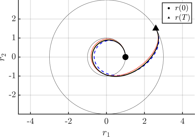
(a) Optimal trajectories in configuration space, $(r_{1},r_{2})$

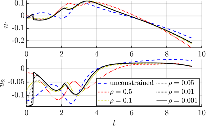
(b) Optimal control profiles

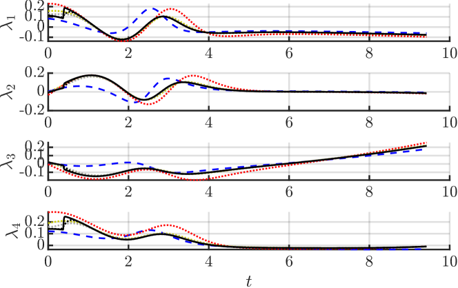
(c) Optimal costate profiles

Figure 2: Numerical example results with various $\rho$. The same legend in (b) applies to (a) and (c).

With this system, the state-constrained optimal control problem we consider is defined as follows:

$$\begin{aligned} L=\frac{1}{2}\left\lVert u\right\rVert_{2}^{2},\ x(0)=x_{0},\ x(T)=x_{T},\ S=p_{\min}-p(x),\end{aligned}$$

where $x_{0},x_{T},T,p_{\min}$ are fixed given parameters, representing the initial state, final state, final time, and the minimum allowable semilatus rectum of the transfer orbit. The semilatus rectum of an orbit, denoted by $p\in\mathbb{R}$, is given by

$$\begin{aligned} p(x)=[l(x)]^{2}/\mu_{g},\quad l(x)=r_{1}v_{2}-r_{2}v_{1}\end{aligned}$$ (42)

where $l\in\mathbb{R}$ represents the magnitude of the orbit angular momentum. Noting that this problem is a special case of the analytical example in Section III-D with $F=B,S_{t}=0,c(\cdot)=0,R=\frac{1}{2}I_{2}$, and $P=0$, the necessary conditions of the optimal trajectory are derived as:

$$\begin{aligned} u^{*}=-B^{\top}(\lambda+\mu^{*}S_{x}^{\top}),\quad\mu^{*}=\frac{S_{x}f_{0}-S_{x}BB^{\top}\lambda}{S_{x}BB^{\top}S_{x}^{\top}}\end{aligned}$$ (43)

The transversality condition is given as $x(T)=x_{T}$ with the initial condition $x(0)=x_{0}$.

The transfer considered is from a circular orbit with radius $1$ to another circular orbit with radius $3$ with the arrival longitude $30$ deg for duration $T=3\pi$, i.e., the following parameters are used: $x_{0}=[1,0,0,1]^{\top},\ x_{T}=[3\sqrt{3}/2,1.5,-1/(2\sqrt{3}),0.5]^{\top},\ T=3\pi,\ p_{\min}=0.9$.

Applying the proposed solution method to this optimal orbit transfer problem leads to Problem 2, which is then numerically solved for the initial costate $\lambda(0)$ by Matlab’s fsolve, where $\rho\ (=\rho_{1}=\rho_{2}=\rho_{3})$ is used with a sequence $\rho=\{0.5,0.1,5.0\times 10^{-2},10^{-2},5.0\times 10^{-3},10^{-3}\}$.

The solution for each $\rho$ is depicted in Fig. 2 with the unconstrained solution included for comparison. It is evident from Figs. 2(b) and 2(c) that both control and costate experience a discontinuity at around $t=0.4$, which is well-modeled by the smooth approximation.

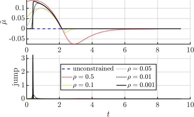
(a) Smooth approximation of discontinuous constraint multiplier and costate jump

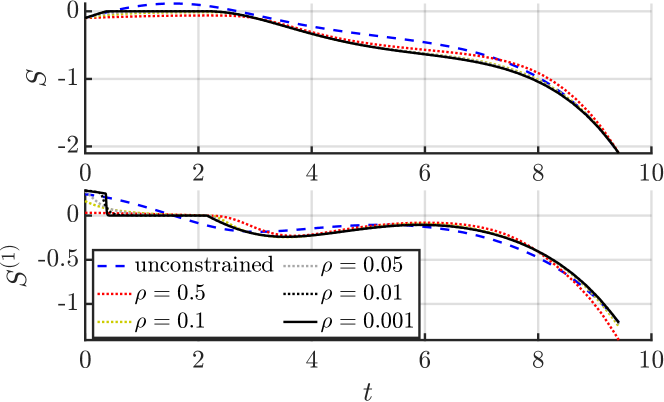
(b) State constraint and its time derivative

Figure 3: Smooth behavior of the numerical example with various $\rho$

Fig. 3 provides further insight into how the proposed solution method behaves for this numerical example. Fig. 3(a) shows the behavior of $\tilde{\mu}^{*}$ (constraint multiplier) and $2\tilde{\mu}^{*}\tilde{\delta}(S)S^{(1)}$ (time derivative of costate jump; see Eq. 40), which numerically verifies the analytical development in Section IV. Fig. 3(b) plots the time history of $S$ and $S^{(1)}$, confirming that every intermediate solution in the continuation respects the state constraint, even for a relatively blunt sharpness parameter $\rho=0.5$ (see Fig. 1), which is, again, often a desirable property for safety-critical applications.

VI Conclusions

In this paper, a new indirect solution method for state-constrained optimal control problems is proposed to address the long-standing issue of discontinuous control and costate due to pure state inequality constraints. The proposed solution method is enabled by re-examining the necessary conditions of optimality for state-constrained optimal control problems with nonlinear control-affine systems and by deriving a unifying form of necessary conditions based on the uniqueness of the optimal control and constraint multiplier on constrained arcs. Unlike classical indirect solution methods for state-constrained optimal control problems, the proposed method transforms the originally discontinuous problems into smooth TPBVPs, eliminating the need of a priori knowledge about the constrained trajectory structure, which is usually unknown. A numerical example demonstrates the proposed method and its favorable properties, including the satisfaction of state constraints at every step of the continuation. An important next direction of this work is to generalize the framework to the case with higher-order state constraints (i.e., the explicit dependency on $u$ first appears at the $p$-th derivative of $S$ with $p>1$).

References

- [1] R. F. Hartl, S. P. Sethi, and R. G. Vickson, “A Survey of the Maximum Principles for Optimal Control Problems with State Constraints,” SIAM Review, vol. 37, pp. 181–218, June 1995.
- [2] A. E. Bryson and Y.-C. Ho, Applied Optimal Control. Routledge, 1975.
- [3] J. L. Speyer and A. E. Bryson, “Optimal programming problems with a bounded state space.,” AIAA Journal, vol. 6, pp. 1488–1491, Aug. 1968.
- [4] H. G. Bock and K. J. Plitt, “A Multiple Shooting Algorithm for Direct Solution of Optimal Control Problems*,” IFAC Proceedings Volumes, vol. 17, pp. 1603–1608, July 1984.
- [5] C. R. Hargraves and S. W. Paris, “Direct Trajectory Optimization Using Nonlinear Programming and Collocation,” Journal of Guidance, Control, and Dynamics, vol. 10, no. 4, pp. 338–342, 1987.
- [6] M. Szmuk, T. P. Reynolds, and B. Açıkmeşe, “Successive Convexification for Real-Time Six-Degree-of-Freedom Powered Descent Guidance with State-Triggered Constraints,” Journal of Guidance, Control, and Dynamics, vol. 43, pp. 1399–1413, Aug. 2020.
- [7] J. Nocedal and S. J. Wright, “Interior-Point Methods for Nonlinear Programming,” in Numerical Optimization, pp. 563–597, New York: Springer New York, 2006.
- [8] Y. Mao, M. Szmuk, and B. Acikmese, “Successive convexification of non-convex optimal control problems and its convergence properties,” in 2016 IEEE 55th Conference on Decision and Control (CDC), pp. 3636–3641, IEEE, Dec. 2016.
- [9] E. F. Camacho and C. Bordons, Model Predictive Control. 2007.
- [10] M. A. Patterson and A. V. Rao, “GPOPS-II: A MATLAB Software for Solving Multiple-Phase Optimal Control Problems Using hp-Adaptive Gaussian Quadrature Collocation Methods and Sparse Nonlinear Programming,” ACM Transactions on Mathematical Software, vol. 41, pp. 1:1–1:37, Oct. 2014.
- [11] H. J. Kelley, “Method of Gradients,” in Optimization Techniques With Applications to Aerospace Systems, vol. 5, pp. 205–254, Academic Press Inc., 1962.
- [12] W. F. DENHAM and A. E. BRYSON, “Optimal programming problems with inequality constraints. ii - solution by steepest-ascent,” AIAA Journal, vol. 2, pp. 25–34, Jan. 1964.
- [13] K. L. Teo and L. S. Jennings, “Nonlinear optimal control problems with continuous state inequality constraints,” Journal of Optimization Theory and Applications, vol. 63, pp. 1–22, Oct. 1989.
- [14] S. P. Han and O. L. Mangasarian, “Exact penalty functions in nonlinear programming,” Mathematical Programming, vol. 17, pp. 251–269, Dec. 1979.
- [15] M. R. Hestenes, “Multiplier and gradient methods,” Journal of Optimization Theory and Applications, vol. 4, pp. 303–320, Nov. 1969.
- [16] D. P. BERTSEKAS, “The Method of Multipliers for Inequality Constrained and Nondifferentiable Optimization Problems,” in Constrained Optimization and Lagrange Multiplier Methods, pp. 158–178, Elsevier, 1982.
- [17] D. Jacobson and M. Lele, “A transformation technique for optimal control problems with a state variable inequality constraint,” IEEE Transactions on Automatic Control, vol. 14, pp. 457–464, Oct. 1969.
- [18] K. Oguri and J. W. McMahon, “Stochastic Primer Vector for Robust Low-Thrust Trajectory Design Under Uncertainty,” Journal of Guidance, Control, and Dynamics, vol. 45, pp. 84–102, Jan. 2022.
- [19] K. Oguri and G. Lantoine, “Stochastic Sequential Convex Programming for Robust Low-thrust Trajectory Design under Uncertainty,” in AAS/AIAA Astrodynamics Conference, pp. 1–20, 2022.
- [20] Y. Sidhoum and K. Oguri, “Indirect Forward-Backward Shooting for Low-thrust Trajectory Optimization in Complex Dynamics,” in AAS/AIAA Space Flight Mechanics Meeting, p. 20, 2023.
- [21] L. S. Pontryagin, V. G. Boltyanskii, R. V. Gamkrelidze, and E. F. Mischenko, The Mathematical Theory of Optimal Processes. CRC Press, 1962.
- [22] A. E. Bryson, W. F. Denham, and S. E. Dreyfus, “Optimal Programming Problems with Inequality Constraints I: Necessary Conditions for Extremal Solutions,” AIAA Journal, vol. 1, pp. 2544–2550, Nov. 1963.
- [23] B. A. Conway, Spacecraft Trajectory Optimization. Cambridge: Cambridge University Press, 2010.
- [24] K. Oguri and J. W. McMahon, “Stochastic Primer Vector for Robust Low-Thrust Trajectory Design Under Uncertainty,” Journal of Guidance, Control, and Dynamics, vol. 45, pp. 84–102, Jan. 2022.
- [25] R. Bonalli, T. Lew, and M. Pavone, “Analysis of Theoretical and Numerical Properties of Sequential Convex Programming for Continuous-Time Optimal Control,” IEEE Transactions on Automatic Control, pp. 1–16, 2022.
- [26] R. Bonalli, A. Bylard, A. Cauligi, T. Lew, and M. Pavone, “Trajectory Optimization on Manifolds: A Theoretically-Guaranteed Embedded Sequential Convex Programming Approach,” in Proceedings of Robotics: Science and Systems, May 2019.
- [27] K. Oguri, M. Ono, and J. W. McMahon, “Convex Optimization over Sequential Linear Feedback Policies with Continuous-time Chance Constraints,” in 2019 IEEE 58th Conference on Decision and Control (CDC), pp. 6325–6331, Dec. 2019.
- [28] L. Cesari, “Lagrange and Bolza Problems of Optimal Control and Other Problems,” in Optimization—Theory and Applications, vol. 10, pp. 196–205, New York, NY: Springer New York, 1983.
- [29] JOHN. McINTYRE and BERNARD. PAIEWONSKY, “On Optimal Control with Bounded State Variables,” in Advances in Control Systems, vol. 5, pp. 389–419, Elsevier, 1967.
- [30] J. Taylor, “Comments on a multiplier condition for problems with state variable inequality constraints,” IEEE Transactions on Automatic Control, vol. 17, pp. 743–744, Oct. 1972.
- [31] E. Taheri and J. L. Junkins, “Generic Smoothing for Optimal Bang-Off-Bang Spacecraft Maneuvers,” Journal of Guidance, Control, and Dynamics, vol. 41, pp. 2470–2475, Nov. 2018.