Successive Convexification with Feasibility Guarantee via Augmented Lagrangian for Non-Convex Optimal Control Problems

Abstract

This paper proposes a new algorithm that solves non-convex optimal control problems with a theoretical guarantee for global convergence to a feasible local solution of the original problem. The proposed algorithm extends the recently proposed successive convexification (SCvx) algorithm by addressing one of its key limitations, that is, the converged solution is not guaranteed to be feasible to the original non-convex problem. The main idea behind the proposed algorithm is to incorporate the SCvx-based iteration into an algorithmic framework based on the augmented Lagrangian method to enable the feasibility guarantee while retaining favorable properties of SCvx. Unlike the original SCvx, this approach iterates on both of the optimization variables and the Lagrange multipliers, which facilitates the feasibility guarantee as well as efficient convergence, in a spirit similar to the alternating direction method of multipliers (ADMM) for large-scale convex programming. Convergence analysis shows the proposed algorithm’s strong global convergence to a feasible local optimum of the original problem and its convergence rate. These theoretical results are demonstrated via numerical examples with comparison against the original SCvx algorithm.

I Introduction

This paper proposes a new algorithm for solving non-convex optimal control problems by extending the successive convexification (SCvx) algorithm [1, 2], a recent algorithm based on sequential convex programming (SCP), and presents a convergence analysis of the proposed algorithm. Most of the real-world problems are non-convex, as seen in aerospace, robotics, and other engineering applications, due to their nonlinear dynamics and/or non-convex constraints. While one can perform lossless convexification for a certain class of problems [3, 4, 5], many remain non-convex. Among various options to tackle those non-convex problems (e.g., [6, 7]), SCP is gaining renewed popularity as a powerful tool, taking advantage of the recent advances in convex programming techniques [8, 1, 2, 9, 10].

Any SCP algorithms take the common approach that repeats the convexify-and-solve processes to march toward a solution of the original problem, which is necessarily a local solution due to the nature of non-convex problems. This concept is shared by many different optimization algorithms, including: sequential linear programming, which is one of the early SCP methods with less computational complexity [11]; difference of convex programming, which decomposes the problem into convex and concave parts while approximating the concave part [12]; and sequential quadratic programming [13], which is adopted in many state-of-the-art nonlinear programming software, such as SNOPT [14].

Among recent SCP algorithms, SCvx [1, 2] (and its specialized version, SCvx-fast [15]) and guaranteed sequential trajectory optimization (GuSTO) [9, 16] are arguably the most notable ones due to their rigorous theoretical underpinnings, with successful applications for various problems [17, 18, 19]. See [8] for a comprehensive review on the recent advances in SCP and other convex programming techniques. In particular, [1] (SCvx) and [16] (GuSTO) analyze the performance of these algorithms in depth, and provide theoretical guarantees on their powerful capabilities, where different approaches are employed in their respective analyses: the Karush–Kuhn–Tucker (KKT) conditions for SCvx while Pontryagin’s minimum principle for GuSTO. On the other hand, like any algorithms, each algorithm has their own limitations, including: the convergence guarantee to a KKT point of the penalty problem but not to the original problem (i.e., lack of feasibility guarantee) in SCvx [1]; the requirement on the dynamical systems to be control-affine in GuSTO [16]. Note that SCvx achieves the convergence to the original problem for a “sufficiently large” penalty weight [1], which the user needs to find by trials and errors.

The objective of this paper is to fill the gap in those theoretical aspects of the existing SCP algorithms by building on the algorithmic foundation laid by SCvx. Specifically, this study proposes a new SCP algorithm that guarantees the convergence to the original non-convex problems while retaining the SCvx’s favorable properties, including the minimal requirements on the dynamical system. The main idea is to incorporate the SCvx-based iteration into an algorithmic framework based on the augmented Lagrangian method (also known as multiplier methods) [20]. The augmented Lagrangian method is a nonlinear programming technique proposed by Hestenes [21] and Powell [22] in 1960s to iteratively improve the Lagrange multiplier estimate, addressing drawbacks of the quadratic penalty method [20].

Based on the augmented Lagrangian framework, the proposed algorithm iterates on the original optimization variables as well as the multipliers of the associated Lagrangian function in the primal-dual formalism. This facilitates the feasibility guarantee as well as efficient convergence, in a spirit similar to the alternating direction method of multipliers (ADMM) for large-scale convex programming [23]. The proposed algorithm is named SCvx*, as it inherits key favorable properties of SCvx and augments it by the newly developed feasibility guarantee, represented by “*”. A preliminary version of SCvx* has been successfully applied to non-convex trajectory optimization problems with covariance control [24, 25] (in fact, SCvx* was the enabler for solving such highly complex control problems), although the present paper is the first to provide the comprehensive, rigorous theoretical convergence analysis of SCvx*.

The main fundamental contributions of the proposed SCvx* algorithm are threefold:

1. provide the convergence guarantee to a feasible local optimum of the original problem, eliminating the need of trials and errors for tuning the penalty weight;

2. provide the strong global convergence to a single local solution of the original problem with minimal requirements on the problem structure; and

3. provide the linear/superlinear convergence rate with a slight modification to the algorithm.

II Preliminary

II-A Problem Statement

We consider solving discrete-time non-convex optimal control problems given by Problem 1, where $x_{s}\in\mathbb{R}^{n_{x}}$ and $u_{s}\in\mathbb{R}^{n_{u}}$ represent the state and control at $s$-th time instance. $g_{\mathrm{affine}}(\cdot)$ and $g_{i}(\cdot)\ \forall i$ represent the affine and non-affine equality constraint functions while $h_{\mathrm{cvx}}(\cdot)$ and $h_{j}(\cdot)\ \forall j$ the convex and non-convex inequality constraint functions. Without loss of generality, $f_{0}(\cdot)$ is assumed convex and continuously differentiable in $x_{s},u_{s}\ \forall s$.

Problem 1 (Non-convex Optimal Control Problem).

$$\begin{aligned} &\underset{x,u}{\min}&&f_{0}(x,u)\\ &\ \mathrm{s.t.}&&x_{s+1}=f_{s}(x_{s},u_{s}),\quad s=1,2,...,N-1,\\ &&&g_{i}(x,u)=0,\quad i=1,2,...,p,\\ &&&h_{j}(x,u)\leq 0,\quad j=1,2,...,q,\\ &&&g_{\mathrm{affine}}(x,u)=0,\quad h_{\mathrm{cvx}}(x,u)\leq 0\end{aligned}$$

where $x=[x_{0}^{\top},x_{1}^{\top},...,x_{N}^{\top}]^{\top}$, $u=[u_{0}^{\top},u_{1}^{\top},...,u_{N-1}^{\top}]^{\top}$.

Defining $z=[x^{\top},u^{\top}]^{\top}\in\mathbb{R}^{n_{z}}$, where $n_{z}=n_{x}(N+1)+n_{u}N$, Problem 1 can be cast as a non-convex optimization problem given in Problem 2, where $g_{i}(\cdot)$ incorporates the dynamical constraints $x_{s+1}=f_{s}(x_{s},u_{s})$.

Problem 2 (Non-convex Optimization Problem).

$$\begin{aligned} &\underset{z}{\min}&&f_{0}(z)\\ &\ \mathrm{s.t.}&&g_{i}(z)=0,\quad i=1,2,...,p+Nn_{x},\\ &&&h_{j}(z)\leq 0,\quad j=1,2,...,q,\\ &&&g_{\mathrm{affine}}(z)=0,\quad h_{\mathrm{cvx}}(z)\leq 0\end{aligned}$$

Define $g_{\mathrm{all}}(\cdot)$ and $h_{\mathrm{all}}(\cdot)$ to represent all the equality and inequality constraints in Problem 2 as: $g_{\mathrm{all}}(z)=[g(z)^{\top},g_{\mathrm{affine}}(z)^{\top}]^{\top}$ and $h_{\mathrm{all}}(z)=[h(z)^{\top},h_{\mathrm{cvx}}(z)^{\top}]^{\top}$, where $g=[g_{1},g_{2},...,g_{p+Nn_{x}}]^{\top}$ and $h=[h_{1},h_{2},...,h_{q}]^{\top}$ are vectorized non-affine and non-convex constraint functions, respectively. Around local solutions of Problem 2, $g_{\mathrm{all}}$ and $h_{\mathrm{all}}$ are assumed to be continuously differentiable and to satisfy the linear independent constraint qualification (LICQ), i.e., the active constraint gradients are linearly independent.

Relevant conditions for a local minimum of Problem 2 are provided in Theorem 1 and Theorem 2. These Theorems are obtained by introducing the Lagrangian function $\mathcal{L}(\cdot)$ with Lagrange multiplier vectors $\lambda$ and $\mu$ as:

$$\mathcal{L}(z,\lambda,\mu)=f_{0}(z)+\lambda^{\top}g_{\mathrm{all}}(z)+\mu^{\top}h_{\mathrm{all}}(z)$$ (1)

and then applying Theorem 12.1 of [6] and Theorem 12.6 of [6] to Problem 2, respectively.

Theorem 1 (First-order Necessary Conditions).

Suppose that $z_{*}$ is a local solution of Problem 2 and that the LICQ holds at $z_{*}$. Then there exist Lagrange multiplier vectors $\lambda_{*}$ and $\mu_{*}$ such that the KKT conditions are satisfied, i.e., $\nabla_{z}\mathcal{L}(z_{*},\lambda_{*},\mu_{*})=0$, $[g_{\mathrm{all}}(z_{*})]_{i}=0$, $[h_{\mathrm{all}}(z_{*})]_{j}\leq 0$, $[\mu_{*}]_{j}\geq 0$, and $[\mu_{*}]_{j}[h_{\mathrm{all}}(z_{*})]_{j}=0,\ \forall i,j$.

Theorem 2 (Second-order Sufficient Conditions).

Suppose that for some feasible point $z_{*}$ of Problem 2, there exist $\lambda_{*}$ and $\mu_{*}$ that satisfy the KKT conditions given in Theorem 1 and that $\nabla_{zz}^{2}\mathcal{L}(z_{*},\lambda_{*},\mu_{*})$ is positive definite on the plane tangent to the constraints, i.e., $v^{\top}\nabla_{zz}^{2}\mathcal{L}(z_{*},\lambda_{*},\mu_{*})v>0,\ \forall v\in\{v\neq 0\mid v^{\top}\nabla_{z}g_{\mathrm{all}}(z_{*})=0,v^{\top}\nabla_{z}h_{\mathrm{active}}(z_{*})=0\}$, where $h_{\mathrm{active}}$ denotes the active inequality constraint vector. Then $z_{*}$ is a strict local solution for Problem 2.

We assume that a local solution $z_{*}$ of Problem 2 together with a unique set of Lagrange multiplier vectors $\lambda_{*}$ and $\mu_{*}$ satisfies the standard second-order sufficient condition for constrained optimization given in Theorem 2.

II-B Augmented Lagrangian Method

The augmented Lagrangian method [20] augments the Lagrangian function Eq. 1 with additional terms parameterized by $w$, defined as:

$$\begin{aligned} \mathcal{L}_{w}(z,\lambda,\mu)=f_{0}(z)+\sum_{i=1}\left\{\lambda_{i}g_{i}+\frac{1}{2}wg_{i}^{2}\right\}\\ +\sum_{j=1}\left\{\mu_{j}h_{j}+\frac{1}{2}w[h_{j}]_{+}^{2}\right\}\end{aligned}$$ (2)

where $[x]_{+}=\max\{0,x\}$, working element-wise if $x$ is a vector. This work takes advantage of the property of the augmented Lagrangian method that guarantees the convergence of the variable $z$ and multipliers $\lambda,\mu$ to the optimum, $z_{*},\lambda_{*},\mu_{*}$, even if the minimization of $\mathcal{L}_{w}(\cdot)$ is inexact at each iteration, provided that a few assumptions are met. Lemma 1 gives a summary of this favorable property and the required assumptions in a form tailored for Problem 2. The superscript $(k)$ denotes the quantities at $k$-th iteration.

Lemma 1 (Augmented Lagrangian Convergence with Inexact Minimization).

Suppose that for Problem 2, a sequence of $\{{z}_{*}^{(k)}\}$ satisfies $\lVert\nabla_{z}\mathcal{L}_{w^{(k)}}({z}_{*}^{(k)},\lambda^{(k)},\mu^{(k)})\rVert_{2}\leq\delta^{(k)}$ where ${\delta^{(k)}}\to 0$ and $\{\lambda^{(k)},\mu^{(k)},w^{(k)}\}$ are updated as:

$$\lambda^{(k+1)}_{i} =\lambda^{(k)}_{i}+w^{(k)}g_{i}({z}_{*}^{(k)}),$$ (3a)

$$\mu^{(k+1)}_{j} =\max\{0,\mu^{(k)}_{j}+w^{(k)}h_{j}({z}_{*}^{(k)})\},$$ (3b)

$$w^{(k+1)} =\beta w^{(k)}\quad(\beta>1)$$ (3c)

where $\{\lambda^{(k)},\mu^{(k)}\}$ are bounded. Then, $w^{(k)}$ eventually exceeds a threshold $w_{*}$ that gives $\nabla_{zz}^{2}\mathcal{L}_{w_{*}}({z}_{*}^{(k)},\lambda^{(k)},\mu^{(k)})\succ 0$, and any sequence $\{{z}_{*}^{(k)},\lambda^{(k)},\mu^{(k)}\}$ globally converges to a local optimum of Problem 2, i.e., $\{{z}_{*}^{(k)},\lambda^{(k)},\mu^{(k)}\}\to\{z_{*},\lambda_{*},\mu_{*}\}$ as $k\to\infty$.

Proof.

The proof is by applying Propositions 2.14, 3.1, and 3.2 of [20] to Problem 2 (see also [26] for an explicit discussion about the global convergence), with the assumption that $\{z_{*},\lambda_{*},\mu_{*}\}$ satisfies the standard second-order sufficient condition given in Theorem 2. ∎

Noting that ${z}_{*}^{(k)}$ represents an approximate minimizer of $\mathcal{L}_{w^{(k)}}(\,\cdot\,,\lambda^{(k)},\mu^{(k)})$, Lemma 1 clarifies that inexact minimization at each augmented Lagrangian iteration must be asymptotically exact, i.e., $\lVert\nabla_{z}\mathcal{L}_{w}(\cdot)\rVert_{2}\to 0$ as $k\to\infty$.

III The Proposed Algorithm

This section describes the proposed algorithm, named SCvx*, that converges to the original problem, Problem 2. The convergence analysis of SCvx* is given in Section IV.

III-A Non-convex Penalty Problem with Augmented Lagrangian

While the augmented Lagrangian function Eq. 2 is introduced from the viewpoint of primal-dual formalism, it can be also viewed from a penalty method standpoint. Adopting this viewpoint, Eq. 2 can be equivalently expressed as $\mathcal{L}_{w}(z,\lambda,\mu)=f_{0}(z)+P(g_{\mathrm{all}}(z),h_{\mathrm{all}}(z),w,\lambda,\mu)$, where $P(g,h,w,\lambda,\mu)$ denotes the penalty function defined as:

$$\begin{aligned} &P(g,h,w,\lambda,\mu)\\ &=\sum_{i=1}\left\{\lambda_{i}g_{i}+\frac{1}{2}wg_{i}^{2}\right\}+\sum_{j=1}\left\{\mu_{j}h_{j}+\frac{1}{2}w[h_{j}]_{+}^{2}\right\}\end{aligned}$$ (4)

With the penalty function of the form given by Eq. 4, we now formulate our non-convex penalty problem based on Problem 2. As our algorithm is based on SCP, our penalty problem penalizes the violations of non-convex constraints only ($\because$ convex constraints are imposed in each convex programming); hence, redefine the Lagrange multipliers as

$$\lambda=[\lambda_{1},\lambda_{2},...,\lambda_{N+p}]^{\top},\quad\mu=[\mu_{1},\mu_{2},...,\mu_{q}]^{\top}\geq 0.$$ (5)

This leads to our non-convex penalty problem, Problem 3.

Problem 3 (Non-convex penalty problem with AL).

$$\begin{aligned} &\underset{z}{\min}&&J(z)=f_{0}(z)+P(g(z),h(z),w,\lambda,\mu)\\ &\quad\mathrm{s.t.}&&g_{\mathrm{affine}}(z)=0,\ h_{\mathrm{cvx}}(z)\leq 0\end{aligned}$$

where $g=[g_{1},g_{2},...,g_{p+Nn_{x}}]^{\top}$ and $h=[h_{1},h_{2},...,h_{q}]^{\top}$.

III-B Convex Penalty Problem with Augmented Lagrangian

Problem 3 is clearly non-convex due to the nonlinearity and non-convexity of $g(\cdot)$ and $h(\cdot)$. To solve the problem via SCP, we linearize them about a reference variable $\bar{z}$ at each iteration, which yields $\widetilde{g}=0$ and $\widetilde{h}\leq 0$, where

$$\begin{aligned} \widetilde{g}(z)&=g(\bar{z})+\nabla_{z}g({\bar{z}})(z-\bar{z}),\\ \widetilde{h}(z)&=h(\bar{z})+\nabla_{z}h({\bar{z}})(z-\bar{z})\end{aligned}$$ (6)

However, imposing $\widetilde{g}=0$ and $\widetilde{h}\leq 0$ in the convex subproblem can lead to the issue of artificial infeasibility [2], and hence these linearized constraints are relaxed as follows:

$$\begin{aligned} \widetilde{g}(z)&=\xi,\quad\widetilde{h}(z)\leq\zeta\end{aligned}$$ (7)

where $\xi=[\xi_{1},\xi_{2},...,\xi_{p+Nnx}]^{\top}$ and $\zeta=[\zeta_{1},\zeta_{2},...,\zeta_{q}]^{\top}\geq 0$. Although the original SCvx literature [2, 1] introduces virtual control and virtual buffer terms separately, the former is naturally incorporated in $\xi$. It is easy to verify this; noting that linearized dynamical constraints are given by

$$\begin{aligned} x_{s+1}=A_{s}x_{s}+B_{s}u_{s}+c_{s}+E_{s}\xi,\quad s=1,2,...,N\end{aligned}$$ (8)

where $E_{s}\in\mathbb{R}^{n_{x}\times p+Nn_{x}}$ extracts the virtual control term at time $t_{s}$ from $\xi$, and

$$\begin{aligned} A_{s}=&\nabla_{x}f_{s}({\bar{x}_{s},\bar{u}_{s}}),\ B_{s}=\nabla_{u}f_{s}({\bar{x}_{s},\bar{u}_{s}}),\\ c_{s}=&f_{s}(\bar{x}_{s},\bar{u}_{s})-A_{s}\bar{x}_{s}-B_{s}\bar{u}_{s}\end{aligned}$$ (9)

it is clear that Eq. 8 can be incorporated into $\widetilde{g}(z)=\xi$.

On the other hand, the linearization and constraint relaxation lead to another issue called artificial unboundedness [1]. To avoid this, we impose a constraint on the variable update magnitude with a trust region bound $r>0$, given by

$$\lVert\bar{z}-z\rVert_{\infty}\leq r$$ (10)

The trust region method is commonly used in many algorithms for nonlinear programming [6].

Problem 4 gives the convex subproblem at each iteration. It is straightforward to verify the convexity of Problem 4 in $z,\xi,\zeta$ by noting that $[x]_{+}^{2}=(\max\{0,x\})^{2}$, which appears in Eq. 4, is convex in $x\in\mathbb{R}$.

Problem 4 (Convex penalty subproblem with AL).

$$\begin{aligned} &\underset{z,\xi,\zeta}{\min}&&L(z,\xi,\zeta)=f_{0}(z)+P(\xi,\zeta,w,\lambda,\mu)\\ &\mathrm{s.t.}\ &&\widetilde{g}(z)=\xi,\ \widetilde{h}(z)\leq\zeta,\ \zeta\geq 0,\\ &&&\lVert\bar{z}-z\rVert_{\infty}\leq r,\ g_{\mathrm{affine}}(z)=0,\ h_{\mathrm{cvx}}(z)\leq 0\end{aligned}$$

III-C SCvx* Algorithm

We are now ready to present the proposed SCvx* algorithm. Algorithm 1 summarizes SCvx*. The key steps of Algorithm 1 are discussed in the rest of this section.

Algorithm 1 SCvx*

Input: $\bar{z}^{(1)},r^{(1)},w^{(1)},\epsilon_{\mathrm{opt}},\epsilon_{\mathrm{feas}},\rho_{0},\rho_{1},\rho_{2},\alpha_{1},\alpha_{2},\beta,\gamma$

1:$k=1$, $\Delta J^{(0)}=\chi^{(0)}=\delta^{(1)}=\infty$, $\lambda^{(1)}=\mu^{(1)}=0$ $\Delta J^{(k-1)}>\epsilon_{\mathrm{opt}}$ or $\chi^{(k-1)}>\epsilon_{\mathrm{feas}}$

2:$\{\widetilde{g}^{(k)},\widetilde{h}^{(k)}\}\leftarrow$ derived via Eq. 6 at $\bar{z}^{(k)}$

3:$\{z^{(k)}_{*},\xi^{(k)}_{*},\zeta^{(k)}_{*}\}\leftarrow$ solve Problem 4

4:$\{\Delta J^{(k)},\Delta L^{(k)},\chi^{(k)}\}\leftarrow$ Eq. 13 $\Delta L^{(k)}=0$

5:$\rho^{(k)}\leftarrow 1$

6:$\rho^{(k)}\leftarrow\Delta J^{(k)}/\Delta L^{(k)}$

7:$\{\bar{z},w,\lambda,\mu,\delta\}^{(k+1)}\leftarrow\{\bar{z},w,\lambda,\mu,\delta\}^{(k)}$ $\triangleright$ default $\rho^{(k)}\geq\rho_{0}$ $\triangleright$ accept the step

8:$\bar{z}^{(k+1)}\leftarrow z^{(k)}_{*}$ $\triangleright$ solution update Eq. 15 is satisfied

9:$\{\lambda,\mu,w\}^{(k+1)}\leftarrow$ Eq. 3 $\triangleright$ multiplier update

10:$\delta^{(k+1)}\leftarrow$ Eq. 16 $\triangleright$ stationarity tol. update

11:$r^{(k+1)}\leftarrow$ Eq. 17 $\triangleright$ trust region update

12:$k\leftarrow k+1$

13:$(z^{(k)}_{*},\lambda^{(k)},\mu^{(k)})$

III-C1 Successive linearization

Let us compactly express the penalty function Eq. 4 at $k$-th iteration as:

$$\begin{aligned} P^{(k)}(g,h)&\triangleq P(g,h,w^{(k)},\lambda^{(k)},\mu^{(k)})\end{aligned}$$ (11)

Likewise, the penalized objectives of Problems 3 and 4 at $k$-th iteration are expressed as:

$$\begin{aligned} J^{(k)}(z)&\triangleq f_{0}(z)+P^{(k)}(g(z),h(z))\\ L^{(k)}(z,\xi,\zeta)&\triangleq f_{0}(z)+P^{(k)}(\xi,\zeta)\end{aligned}$$ (12)

Given a user-provided initial reference point $\bar{z}^{(1)}$, each linearization process follows the one described in Section III-B, which instantiates Problem 4 at each iteration. Problem 4 is solved to convergence, yielding the solution at $k$-th iteration, denoted by $z^{(k)}_{*},\xi^{(k)}_{*},\zeta^{(k)}_{*}$.

Every time after Problem 4 is solved, SCvx* calculates the following quantities:

$$\Delta J^{(k)} =J^{(k)}(\bar{z}^{(k)})-J^{(k)}(z^{(k)}_{*})$$ (13a)

$$\Delta L^{(k)} =J^{(k)}(\bar{z}^{(k)})-L^{(k)}(z^{(k)}_{*},\xi^{(k)}_{*},\zeta^{(k)}_{*})$$ (13b)

$$\chi^{(k)} =\lVert g(z^{(k)}_{*}),[h(z^{(k)}_{*})]_{+}\rVert_{2}$$ (13c)

where $\Delta J^{(k)}$ and $\Delta L^{(k)}$ represent the actual and predicted cost reductions, respectively, while $\chi^{(k)}$ represents the infeasibility of the problem.

III-C2 Step acceptance

After each convex programming, SCvx* accepts the solution and updates $\bar{z}^{(k)}$ if a certain criterion is met. With a user-defined parameter $\rho_{0}\in(0,1)$, the step acceptance criterion is given by

$$\begin{aligned} \rho_{0}\leq\rho^{(k)},\quad\rho^{(k)}={\Delta J^{(k)}}/{\Delta L^{(k)}}\end{aligned}$$ (14)

$\rho^{(k)}$ measures the the relative decrease of the objective, and an iteration is accepted only if the ratio is greater than a prescribed value, which helps avoid accepting bad steps (e.g., those which do not improve the non-convex objective). The acceptance criteria is based on the one proposed in the original SCvx [2], but not exactly the same; this point is made precise in the following remark.

Remark 1.

The definition of $\Delta L^{(k)}$ in Eq. 13b is different from the one in the original SCvx [1, 2]. As SCvx considers a fixed penalty weight, their definition of $\Delta L$ with our notation would correspond to $J^{(k-1)}(\bar{z}^{(k)})-L^{(k)}(z^{(k)}_{*},\xi^{(k)}_{*},\zeta^{(k)}_{*})$, which is not always non-negative because $J^{(k)}(\bar{z}^{(k)})\neq J^{(k-1)}(\bar{z}^{(k)})$. With the careful definition of $\Delta L^{(k)}$ as in Eq. 13b, a key result $\Delta L^{(k)}\geq 0$ is guaranteed in SCvx*, as proved later in Lemma 3.

III-C3 Lagrange multiplier update

Although the Lagrange multipliers $\lambda$ and $\mu$ are fixed when solving each convex subproblem, they must be updated to march toward the convergence of the original problem (Problem 2), i.e., $\{z^{(k)},\lambda^{(k)},\mu^{(k)}\}\to\{z_{*},\lambda_{*},\mu_{*}\}$, which facilitates the feasibility to Problem 2. In SCvx*, $\lambda$ and $\mu$ are updated when the current iteration is accepted (i.e., $\rho^{(k)}\geq\rho_{0}$) and the following condition is met:

$$\begin{aligned} \lvert\Delta J^{(k)}\rvert<\delta^{(k)},\end{aligned}$$ (15)

where $\delta^{(k)}$ is updated such that $\delta^{(k)}\to 0$ as $k\to\infty$, satisfying the asymptotically exact minimization requirement for the augmented Lagrangian method to converge (see Lemma 1). A simple design is to update $\delta^{(k)}$ as:

$$\delta^{(k+1)}=\begin{cases}\lvert\Delta J^{(k)}\rvert&\mathrm{if}\ \delta^{(k)}=\infty\\ \gamma\delta^{(k)}&\mathrm{otherwise}\quad\quad(\gamma\in(0,1))\end{cases}$$ (16)

when Eq. 15 is met. SCvx* initializes $\delta^{(k)}$ as $\delta^{(1)}=\infty$ by default, although if one has a good estimate of $\delta^{(1)}$, then one can use it to initialize $\delta^{(k)}$ instead of using $\infty$.

Every time when Eq. 15 is met, SCvx* performs an update to $w^{(k)},\lambda^{(k)},\mu^{(k)}$ using Eq. 3, where $g_{i}(\cdot)$ and $h_{j}(\cdot)$ in Eq. 3 must refer to the non-convex constraint functions. As formally proved in Section IV-A, this scheme ensures satisfying the convergence conditions in Lemma 1. A stricter condition than Eq. 15 is also possible that provides superlinear convergence rate, as discussed in Section IV-B.

III-C4 Trust region update

The trust region radius $r$ plays a key role in preventing artificial unboundedness. $\rho^{(k)}$ introduced in Eq. 14 is used to quantify the quality of the current radius $r^{(k)}$ and update it according to a criterion. Like original SCvx [2], given the user-defined initial radius $r^{(1)}>0$ and thresholds $\rho_{1}$, $\rho_{2}$ that satisfy $\rho_{0}<\rho_{1}<\rho_{2}$, SCvx* updates $r^{(k)}$ as follows:

$$r^{(k+1)}=\begin{cases}\max\{r^{(k)}/\alpha_{1},r_{\min}\}&\mathrm{if}\ \rho^{(k)}<\rho_{1}\\ r^{(k)}&\mathrm{elseif}\ \rho^{(k)}<\rho_{2}\\ \min\{\alpha_{2}r^{(k)},r_{\max}\}&\mathrm{else}\end{cases}$$ (17)

where $\alpha_{1}>1$ and $\alpha_{2}>1$ determine the contracting and enlarging ratios of $r^{(k)}$, respectively. The lower and upper bounds of $r^{(k)}$ are given by $r_{\min}$ and $r_{\max}$, respectively, with $r_{\max}>r_{\min}>0$; taking $r_{\max}=\infty$ (i.e., no upper bound) does not affect the convergence property.

III-C5 Convergence check

SCvx* detects the convergence to Problem 2 and terminates the iteration if the following condition is met:

$$\Delta J^{(k)}\leq\epsilon_{\mathrm{opt}}\quad\land\quad\chi^{(k)}\leq\epsilon_{\mathrm{feas}}$$ (18)

where $\epsilon_{\mathrm{opt}}$ and $\epsilon_{\mathrm{feas}}$ are small positive user-defined parameters representing the optimality and feasibility tolerances.

IV Convergence Analysis

This section presents the convergence analysis of SCvx*. Section IV-A shows the global strong convergence to the original problem, Problem 2, while Section IV-B discusses its convergence rate.

IV-A Convergence

Let us first introduce Lemma 2, which provides the local optimality necessary condition for Problem 3.

Lemma 2 (Local Optimality Necessary Condition).

If $z_{*}$ is a local minimizer of $J^{(k)}$ in Problem 3, then $z_{*}$ is a stationary point of $J^{(k)}$ with the current $w^{(k)},\lambda^{(k)},\mu^{(k)}$.

Proof.

Apply Theorem 2.2 of [6] to Problem 3. ∎

We then present Lemma 3, which states the non-negativity of $\Delta L^{(k)}$ as well as the stationarity of $J^{(k)}$ when $\Delta L^{(k)}=0$. This extends Theorem 3 of [2] (also Theorem 3.10 of [1]) to account for the effect of varying $w^{(k)},\lambda^{(k)},\mu^{(k)}$ due to the augmented Lagrangian framework.

Lemma 3.

The predicted cost reductions $\Delta L^{(k)}$ in Eq. 13b satisfy $\Delta L^{(k)}\geq 0$ for all $k$. Also, $\Delta L^{(k)}=0$ implies that the reference point $z=\bar{z}^{(k)}$ is a stationary point of $J^{(k)}$.

Proof.

Since $(z^{(k)}_{*},\xi^{(k)}_{*},\zeta^{(k)}_{*})$ solves Problem 4, we have

$$\begin{aligned} L^{(k)}(z^{(k)}_{*},\xi^{(k)}_{*},\zeta^{(k)}_{*})\leq L^{(k)}(\bar{z}^{(k)},g(\bar{z}^{(k)}),h(\bar{z}^{(k)}))\\ =f_{0}(\bar{z}^{(k)})+P^{(k)}(g(\bar{z}^{(k)}),h(\bar{z}^{(k)}))=J^{(k)}(\bar{z}^{(k)})\end{aligned}$$ (19)

Thus, it implies that $\Delta L^{(k)}\geq 0$ for all $k$ and that $\Delta L^{(k)}=0$ holds if and only if $z^{(k)}_{*}=\bar{z}^{(k)}$. From this, $\Delta L^{(k)}=0$ implies that $z=\bar{z}^{(k)}$ is a local minimizer of $J^{(k)}$, and hence, from Lemma 2, a stationary point of $J^{(k)}$. ∎

Lemma 3 is a key for SCvx* to inherit two favorable aspects of the original SCvx algorithm, namely, (1) the assured acceptance of iteration and (2) the assured stationarity of limit points. Lemmas 4 and 5 clarify these two aspects in the context of SCvx* by extending those of SCvx.

Lemma 4.

The SCvx* iterations are guaranteed to be accepted (i.e., Line 7 is satisfied) within a finite number of iterations after an iteration is rejected.

Proof.

It is straightforward to prove this by combining Lemmas 3 and 2 and the proof for Lemma 3 of [2] (or Lemma 3.11 of [1]), where the generalized differential and the generalized directional derivative can be replaced with the gradient and directional derivative ($\because$ unlike SCvx, the penalty function of SCvx* is differentiable due to the formulation based on the augmented Lagrangian method). ∎

Lemma 5.

A sequence $\{z^{(k)}_{*}\}$ generated by SCvx* when the Lagrange multipliers and penalty weight are fixed is guaranteed to have limit points, and any limit point $\hat{z}$ is a stationary point of Problem 3.

Proof.

It is straightforward to prove by combining Lemmas 3 and 4 and the proof for Theorem 4 of [2] (or Theorem 3.13 of [1]), where note from Eq. 17 that the trust region satisfies $r^{(k)}\geq r_{\min}>0$. ∎

Remarkably, Lemma 5 implies that, when the values of $\lambda^{(k)},\mu^{(k)},w^{(k)}$ remain fixed, we have $\Delta J^{(k_{i})}\to 0$ as $i\to\infty$, where $\{z_{*}^{(k_{i})}\}$ is a subsequence of $\{z_{*}^{(k)}\}$. This assures the satisfaction of Line 8 within a finite (typically a few) number of iterations after $\lambda^{(k)},\mu^{(k)},w^{(k)}$ are last updated. This key property is formally stated in Lemma 6.

Lemma 6.

The SCvx* multipliers and penalty weights are guaranteed to be updated (i.e., Line 8 is satisfied) within a finite number of iterations after their last update.

Proof.

The proof is by contradiction. Suppose that Line 8 is not satisfied for indefinite number of iterations, i.e., $\lvert\Delta J^{(k)}\rvert\geq\delta^{(k)}$ for $k\to\infty$. Since $\lvert\Delta J^{(k)}\rvert\geq\delta^{(k)}$, the multipliers and penalty weight $\lambda^{(k)},\mu^{(k)},w^{(k)}$ remain the same for $k\to\infty$. However, when $\lambda^{(k)},\mu^{(k)},w^{(k)}$ remain the same values, there are at least one subsequence with $\Delta J^{(k_{i})}\to 0$ due to Lemma 5, which eventually satisfies $\lvert\Delta J^{(k)}\rvert<\delta^{(k)}$ for any $\delta^{(k)}>0$ without requiring infinite $k$. This contradicts $\lvert\Delta J^{(k)}\rvert\geq\delta^{(k)}$ for $k\to\infty$, and therefore implies Lemma 6. ∎

We are now ready to present the main result of this paper on the convergence property of the SCvx* algorithm.

Theorem 3 (Global Strong Convergence with Feasibility).

SCvx* achieves global convergence to a feasible local optimum of the original problem, Problem 2.

Proof.

Let $\{z^{(k_{i})}_{*}\}$ be a subsequence of $\{z^{(k)}_{*}\}$ that consists of the iterations where the multipliers are updated; such subsequences are guaranteed to exist due to Lemma 6. Then, Eq. 16 ensures $\delta^{(k_{i})}>\delta^{(k_{i}+1)}$, and due to Lemma 5, $\Delta J^{(k_{i})}\to 0$ and $\delta^{(k_{i})}\to 0$ in the limit. Again due to Lemma 5, the limit point is a stationary point of Problem 3, satisfying $\nabla_{z}J^{(k)}=0$. Then, $\nabla_{z}\mathcal{L}_{w^{(k)}}\to 0$ also holds in the limit since every $z^{(k)}_{*}$ satisfies $g_{\mathrm{affine}}=0$ and $h_{\mathrm{cvx}}\leq 0$ within the convex programming. Thus, the SCvx* iteration guarantees $\lVert\nabla_{z}\mathcal{L}_{w^{(k)}}\rVert_{2}\to 0$ in the limit, with the multiplier update Eq. 3. Therefore, as $w^{(k)}$ exceeds the threshold $w_{*}$ given in Lemma 1 after finite iterations, SCvx* achieves the global convergence to a feasible optimum of Problem 2. ∎

Remarks below discuss two key improvements that the SCvx* algorithm provides over the original SCvx algorithm. Note also that original SCvx requires the assumptions on the penalized cost function to satisfy the Kurdyka–Lojasiewicz properties [27] for the global strong convergence [1].

Remark 2 (Feasibility).

The converged solution generated by SCvx* is feasible to Problem 2, while the original SCvx algorithm does not provide such a feasibility guarantee.

Remark 3 (Accelerated convergence).

SCvx* iterates not only on the variable $z^{(k)}$ but also on the Lagrange multipliers $\lambda^{(k)}$ and $\mu^{(k)}$, which, besides providing the feasibility guarantee, facilitates the convergence by iteratively improving the multiplier estimate rather than using a fixed value.

IV-B Convergence rate

Having the augmented Lagrangian method as the basis of the algorithm facilitates the analysis of the convergence rate of SCvx*. Based on [20, 26], linear or superlinear convergence rate of the augmented Lagrangian method can be achieved when the multiplier update tolerance $\delta^{(k)}$ decreases to zero as fast as $\lVert\lambda^{(k)}-\lambda_{*}\rVert_{2}/w^{(k)}$. To achieve this, we may replace Eq. 15 by a stronger condition:

$$\lvert\Delta J^{(k)}\rvert\leq\min{\{\delta^{(k)},\eta\chi^{(k)}\}},$$ (20)

where $\eta$ is a positive scalar. With this criterion, Proposition 2 of [26] states that the augmented Lagrange multiplier iteration Eq. 3 converges to $z_{*},\lambda_{*},\mu_{*}$ superlinearly if $w^{(k)}\to\infty$, and linearly if $w^{(k)}\to w_{\max}<\infty$, where $w_{\max}\in(0,\infty)$ is the upper bound of the penalty weight.

The choice of $\eta$ can be arbitrary to achieve the above convergence rate in theory. A simple yet effective approach is to initialize $\eta$ by $\infty$ at first, and then update it by $\eta\leftarrow\lvert\Delta J^{(k)}\rvert/\chi^{(k)}$ when Eq. 20 is met for the first time.

An undesirable situation is that the SCvx* algorithm loses the favorable property of the guaranteed multiplier update (Lemma 6) due to the introduction of the stricter condition Eq. 20. Lemma 7 addresses this concern by stating that a similar guarantee is retained when using Eq. 20 instead of Eq. 15. Once the convergence in $\lambda,\mu$ is achieved, then $\lambda,\mu$ will not be updated anymore, and $z^{(k)}$ converges to a feasible local minimum of Problem 2 due to Lemmas 1 and 5.

Lemma 7.

Suppose that Eq. 20 instead of Eq. 15 is used for the multiplier update criterion. Then, until the convergence in $\lambda$ and $\mu$ is achieved, the SCvx* iteration guarantees that the values of $\lambda$ and $\mu$ are updated within a finite number of iterations after their last update.

Proof.

For conciseness, the proof is focused on problems with equality constraints only, as any inequality constraints can be converted to equality constraints by introducing dummy variables without changing the results in the augmented Lagrangian framework (see Section 3.1 of [20]). Thus, $\mu$ and $h_{j}$ are not explicitly considered in this proof.

It is clear from Lemma 5 that the claim is true if $\chi^{(k)}>0$ holds until the convergence in $\lambda$ is achieved. It is also clear that $\lambda^{(k)}\neq\lambda_{*}$ until the convergence in $\lambda$ is achieved. Thus, let us show $\chi^{(k)}>0$ when $\lambda^{(k)}\neq\lambda_{*}$ by contradiction.

Suppose that there exists certain $\lambda^{(k)}(\neq\lambda_{*})$ such that lead to $\chi^{(k)}=0$. For $z^{(k)}_{*}$ that solves Problem 4, it is clear from Eq. 13c that $\chi^{(k)}=0$ if and only if $g(z^{(k)}_{*})=0$. Since $\chi^{(k)}=0$, Eq. 20 is not satisfied, and hence the values of $\lambda^{(k)}$ remain fixed until $\Delta J^{(k)}=0$ is achieved in the limit. Due to Lemma 5, the limit point is a stationary point of Problem 3, satisfying

$$\begin{aligned} 0=\nabla_{z}J^{(k)}=\nabla_{z}f_{0}&+\sum_{i=1}(\lambda_{i}+wg_{i})\nabla_{z}g_{i}\end{aligned}$$ (21)

Using $g=0$ due to $\chi^{(k)}=0$, this leads to

$$\begin{aligned} 0=\nabla_{z}f_{0}+\sum_{i=1}\lambda_{i}\nabla_{z}g_{i}\end{aligned}$$ (22)

which implies that the limit point of $\{z^{(k)}_{*}\}$ is a feasible stationary point of Problem 2, i.e., $\nabla_{z}\mathcal{L}=0$, and hence satisfies the KKT conditions of Problem 2, since every $z^{(k)}_{*}$ also satisfies $g_{\mathrm{affine}}=0$ and associated multiplier conditions within the convex programming. This contradicts $\lambda^{(k)}\neq\lambda_{*}$, and thus $\chi^{(k)}\neq 0$ by contradiction, implying $\chi^{(k)}>0$ because $\chi^{(k)}$ must be non-negative. ∎

To avoid creating false impressions, it is worth emphasizing that the linear/superlinear convergence rate is with respect to the Lagrange multiplier update iteration but not with respect to $k$. In terms of the convergence rate with respect to $k$, it is empirically demonstrated that SCvx* achieves at least the same (often faster) convergence rate as the original SCvx algorithm, with a key additional benefit of convergence to a solution of Problem 2 instead of Problem 3, which is due to the convergence in $\lambda$ and $\mu$.

V Numerical Examples

This section presents two numerical examples to demonstrate the proposed SCvx* algorithm and compare the performance against the conventional SCvx. Note that Algorithm 1 boils down to SCvx by ignoring Lines 8 to 10 and replacing the penalty function Eq. 4 by an $l_{1}$-norm exact penalty function $P(g,h,w)=w\lVert g\rVert_{1}+w\sum_{j}[h_{j}]_{+}$. Each convex subproblem is solved via CVX [28] with Mosek [29].

The SCvx* parameters commonly used for the two examples are listed in Table I. In each example, $w^{(1)}$ is varied to investigate the performance of SCvx* and SCvx for different penalty weights. $w_{\max}=10^{8}$ is set for SCvx* to avoid potential numerical issues, although none of the test cases achieved this maximum value except for the two cases in Example 1 (with $w^{(1)}=10^{4},10^{5}$). $r^{(1)}=0.1,\ r_{\min}=10^{-10},\ r_{\max}=10$ are used for trust region. If the algorithm does not converge in $100$ iterations, it is terminated and deemed unconverged.

Table I: SCvx* parameters ($\epsilon=\epsilon_{\mathrm{opt}}=\epsilon_{\mathrm{feas}}$)

Parameter	$\epsilon$	$\{\rho_{0},\rho_{1},\rho_{2}\}$	$\{\alpha_{1},\alpha_{2}\}$	$\beta$	$\gamma$
Value	$10^{-5}$	$\{0.0,0.25,0.7\}$	$\{2.0,3.0\}$	$2.0$	$0.9$

V-A Example 1: Simple Problem with Crawling Phenomenon

The first example is a simple non-convex optimization problem from [30] to demonstrate that SCvx* can also overcome the so-called crawling phenomenon, which is known to occur for a class of SCP algorithms. According to [30], original SCvx belongs to the class $\mathcal{A}_{C}$ and thus is susceptible to the crawling phenomenon, while SCvx* does not belong to $\mathcal{A}_{C}$ due to the different form of the penalty function. The non-convex problem from [30] is defined in the form of Problem 2 as follows:

$$\underset{-2\leq z\leq 2}{\min} z_{1}+z_{2}$$ (23a)

$$\ \mathrm{s.t.} z_{2}-z_{1}^{4}-2z_{1}^{3}+1.2z_{1}^{2}+2z_{1}=0,$$ (23b)

$$-z_{2}-\frac{4}{3}z_{1}-\frac{2}{3}\leq 0$$ (23c)

which is solved by SCvx* and SCvx with various $w^{(1)}$. The same initial reference point as [30], $\bar{z}^{(1)}=[1.5,1.5]$, is used.

Table II summarizes the comparison of SCvx* and SCvx by listing the number of iterations required for convergence with respect to different values of $w^{(1)}$. “N/A” indicates non-convergence achieved within the maximum iteration limit (=100). Table II illustrates that SCvx* constantly achieves the convergence regardless of the initial values of $w^{(k)}$, even for a small initial weight, $w^{(1)}=0.1$; this is in sharp contrast to the SCvx results, which successfully converge to a feasible local minimum only for the two cases: $w^{(1)}=10$ and $100$, emphasizing the sensitivity to the value of $w^{(1)}$ (which is held constant over iterations in SCvx).

Fig. 1 depicts the convergence behavior for $w^{(1)}=1$. This figure clarifies that the SCvx* iteration successfully converges to the optimum while SCvx is not able to satisfy the non-convex equality constraint (on the black curve).

It is observed from this example that non-converging modes of SCvx can be categorized into two modes:

1. non-improving infeasibility (for $w^{(1)}=10^{-1},10^{0}$);

2. crawling phenomenon (for $w^{(1)}=10^{3},10^{4},10^{5}$).

Table II: Example 1: Convergence Results with Different Initial Penalty Weights (N/A indicates non-convergence)

$w^{(1)}$ value	$10^{-1}$	$10^{0}$	$10^{1}$	$10^{2}$	$10^{3}$	$10^{4}$	$10^{5}$
SCvx* # ite.	39	33	31	42	40	51	56
SCvx # ite.	N/A	N/A	35	31	N/A	N/A	N/A

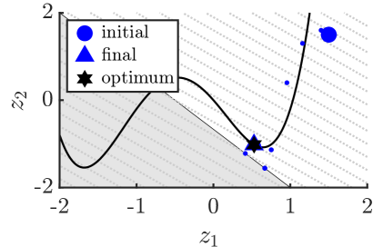
(a) SCvx* result, 33 iterations

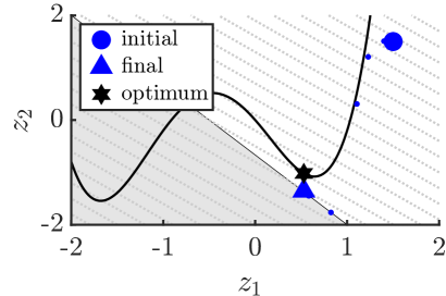
(b) SCvx result, not converged

Figure 1: Example 1 convergence behavior for $w^{(1)}=1$ in the $z_{1}$-$z_{2}$ space. The black curve represents the non-convex equality constraint Eq. 23b, and the gray shaded area is the infeasible area from Eq. 23c.

On the other hand, SCvx* effectively addresses both of the non-converging modes, consistent with the two key improvements over SCvx discussed in Remarsks 2 and 3.

V-B Example 2: Quad Rotor Path Planning

The second example is a quad-rotor non-convex optimal control problem from the original SCvx literature [1]. The problem is defined in the form of Problem 1 as follows:

$$\begin{aligned} &\underset{x,u}{\min}&&\sum_{s=1}^{N}\Gamma_{s}\Delta t\\ &\ \mathrm{s.t.}&&x_{s+1}=x_{s}+\int_{t_{s}}^{t_{s+1}}\begin{bmatrix}v\\ \frac{1}{m}T-k_{D}\lVert v\rVert_{2}v+g\end{bmatrix}\mathrm{d}t,\ \forall s\\ &&&\lVert p_{s}-p_{\mathrm{obj},j}\rVert_{2}\geq R_{\mathrm{obs},j},\quad j=1,2,\\ &&&x_{1}=x_{\mathrm{ini}},\ x_{N}=x_{\mathrm{fin}},\ T_{1}=T_{N}=-mg,\\ &&&[1\ 0\ 0]\cdot p_{s}=0,\ \lVert T_{s}\rVert_{2}\leq\Gamma_{s},\ T_{\min}\leq\Gamma_{s}\leq T_{\max},\\ &&&\cos{\theta_{\max}}\Gamma_{s}\leq[1\ 0\ 0]\cdot T_{s},\quad\forall s\end{aligned}$$

where $p\in\mathbb{R}^{3}$, $v\in\mathbb{R}^{3}$, and $m\in\mathbb{R}$ denote the position, velocity, and mass of the vehicle; $T\in\mathbb{R}^{3}$ is the thrust vector; $\Gamma\in\mathbb{R}$ is an auxiliary variable representing the thrust magnitude (at convergence); $g=[-9.81,0,0]^{\top}\,\mathrm{m/s^{2}}$ is the gravity acceleration; $k_{D}=0.5$ is the drag coefficient; $p_{\mathrm{obj},j}$ and $R_{\mathrm{obj},j}$ are the position and radius of $j$-th obstacle (defined the same as [1]); $x_{\mathrm{ini}}=[0\,\mathrm{m},\ 0\,\mathrm{m},\ 0\,\mathrm{m},\ 0\,\mathrm{m/s},\ 0.5\,\mathrm{m/s},\ 0\,\mathrm{m/s}]^{\top}$ and $x_{\mathrm{fin}}=[0\,\mathrm{m},\ 10\,\mathrm{m},\ 0\,\mathrm{m},\ 0\,\mathrm{m/s},\ 0.5\,\mathrm{m/s},\ 0\,\mathrm{m/s}]^{\top}$ are the initial and final states; $T_{\min}=1.0$ N and $T_{\max}=4.0$ N are the minimum and maximum thrust; $\theta_{\max}=45$ degree is the maximum tilt angle of the thrust vector. The state and control variables are $x_{s}=[r_{s}^{\top},v_{s}^{\top}]^{\top}\in\mathbb{R}^{6}$ and $u_{s}=[T_{s}^{\top},\Gamma_{s}]^{\top}\in\mathbb{R}^{4}$, where the zeroth-order-hold control is used for the discretization, i.e., $u_{s}=u(t)\ \forall t\in[t_{s},t_{s+1})$. The final time is $t_{N}=5.0$ seconds, with time discretization $N=31$. To initialize $\bar{z}^{(1)}$, the straight line that connects $x_{\mathrm{init}}$ and $x_{\mathrm{fin}}$ is used for $x_{s}$ while $-mg$ and $\lVert mg\rVert_{2}$ are used for $T_{s}$ and $\Gamma_{s}$, respectively.

Table III: Example 2: Convergence Results

$w^{(1)}$ value	$10^{-1}$	$10^{0}$	$10^{1}$	$10^{2}$	$10^{3}$	$10^{4}$	$10^{5}$
SCvx* # ite.	24	17	14	11	11	11	14
SCvx # ite.	N/A	9	11	13	14	15	16

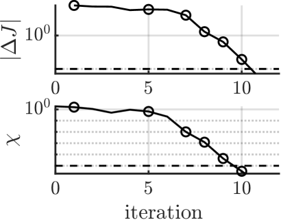
(a) SCvx* result, 11 iterations

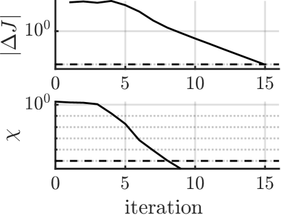
(b) SCvx result, 15 iterations

Figure 2: Example 2 convergence behavior for $w^{(1)}=10^{4}$, in terms of the penalized objective improvement $\lvert\Delta J^{(k)}\rvert$ and the infeasibility $\chi^{(k)}$. The circles in (a) indicate the iterations with multiplier updates.

Table III summarizes the convergence results for Example 2. This suggests that the performance of SCvx* and SCvx are similar overall for this example, although a key difference is observed that SCvx struggles to converge to a feasible solution when $w^{(1)}=10^{-1}$. SCvx* constantly converges to a feasible local minimum regardless of $w^{(1)}$ without needing to worry about the penalty weight. This property can be highly valuable for large-scale optimization problems, where the user may not afford to tune the penalty weight value (e.g., those involving covariance control and multiple phases [24]). On the other hand, this also provides a reassuring result that, despite the lack of the theoretical feasibility guarantee, SCvx can also perform very well and may be good enough for relatively simple, small-scale optimal control problems.

Fig. 2 presents the convergence behavior for $w^{(1)}=10^{4}$ in terms of the two criteria used for the convergence detection. The circles in Fig. 2(a) indicate the iterations when Line 8 of Algorithm 1 is satisfied and the multipliers are updated. The dashed lines represent the tolerance $\epsilon=\epsilon_{\mathrm{opt}}=\epsilon_{\mathrm{feas}}(=10^{-5})$. While SCvx satisfies the constraints earlier, SCvx* achieves the overall convergence faster, which would be due to the iterative estimate of Lagrange multipliers that balances the progress in optimality and feasibility.

VI Conclusions

In this paper, a new SCP algorithm SCvx* is proposed to address the lack of feasibility guarantee in SCvx by leveraging the augmented Lagrangian framework. Unlike SCvx, which uses a fixed penalty weight over iterations, SCvx* iteratively improves both of the optimization variables and the Lagrange multipliers, facilitating the convergence. Inheriting the favorable properties of SCvx and fusing those with the augmented Lagrangian method, SCvx* provides strong global convergence to a feasible local optimum of the original non-convex optimal control problems with minimal requirements on the problem form. The convergence rate of SCvx* is also analyzed, clarifying that linear/superlinear convergence rate can be achieved by slightly modifying the algorithm. These theoretical results are demonstrated via numerical examples.

References

- [1] Y. Mao, M. Szmuk, X. Xu, and B. Acikmese, “Successive Convexification: A Superlinearly Convergent Algorithm for Non-convex Optimal Control Problems,” arXiv preprint, Feb. 2019.
- [2] Y. Mao, M. Szmuk, and B. Acikmese, “Successive convexification of non-convex optimal control problems and its convergence properties,” in 2016 IEEE 55th Conference on Decision and Control (CDC), pp. 3636–3641, IEEE, Dec. 2016.
- [3] B. Acikmese and S. R. Ploen, “Convex Programming Approach to Powered Descent Guidance for Mars Landing,” Journal of Guidance Control and Dynamics, vol. 30, no. 5, p. 1353, 2007.
- [4] B. Açıkmeşe and L. Blackmore, “Lossless convexification of a class of optimal control problems with non-convex constraints,” Automatica, vol. 47, no. 2, pp. 341–347, 2011.
- [5] M. W. Harris, “Optimal Control on Disconnected Sets Using Extreme Point Relaxations and Normality Approximations,” IEEE Transactions on Automatic Control, vol. 66, pp. 6063–6070, Dec. 2021.
- [6] J. Nocedal and S. J. Wright, Numerical Optimization. Springer New York, 2006.
- [7] D. Simon, Evolutionary Optimization Algorithms. John Wiley & Sons, Incorporated, 2013.
- [8] D. Malyuta, T. P. Reynolds, M. Szmuk, T. Lew, R. Bonalli, M. Pavone, and B. Açıkmeşe, “Convex Optimization for Trajectory Generation: A Tutorial on Generating Dynamically Feasible Trajectories Reliably and Efficiently,” IEEE Control Systems Magazine, vol. 42, pp. 40–113, Oct. 2022.
- [9] R. Bonalli, A. Cauligi, A. Bylard, and M. Pavone, “GuSTO: Guaranteed Sequential Trajectory optimization via Sequential Convex Programming,” in 2019 International Conference on Robotics and Automation (ICRA), vol. 2019-May, pp. 6741–6747, IEEE, May 2019.
- [10] S. Boyd and L. Vandenberghe, Convex Optimization. Cambridge, England: Cambridge University Press, Mar. 2004.
- [11] F. Palacios-Gomez, L. Lasdon, and M. Engquist, “Nonlinear Optimization by Successive Linear Programming,” Management Science, Oct. 1982.
- [12] A. L. Yuille and A. Rangarajan, “The Concave-Convex Procedure (CCCP),” in Advances in Neural Information Processing Systems, 2003.
- [13] P. T. Boggs and J. W. Tolle, “A Strategy for Global Convergence in a Sequential Quadratic Programming Algorithm,” SIAM Journal on Numerical Analysis, vol. 26, pp. 600–623, June 1989.
- [14] P. E. Gill, W. Murray, and M. A. Saunders, “SNOPT: An SQP Algorithm for Large-Scale Constrained Optimization,” SIAM Journal on Optimization, vol. 12, pp. 979–1006, Jan. 2002.
- [15] Y. Mao and B. Acikmese, “SCvx-fast: A Superlinearly Convergent Algorithm for A Class of Non-Convex Optimal Control Problems,” pp. 1–22, Nov. 2021.
- [16] R. Bonalli, T. Lew, and M. Pavone, “Analysis of Theoretical and Numerical Properties of Sequential Convex Programming for Continuous-Time Optimal Control,” IEEE Transactions on Automatic Control, pp. 1–16, 2022.
- [17] M. Szmuk, T. P. Reynolds, and B. Açıkmeşe, “Successive Convexification for Real-Time Six-Degree-of-Freedom Powered Descent Guidance with State-Triggered Constraints,” Journal of Guidance, Control, and Dynamics, vol. 43, pp. 1399–1413, Aug. 2020.
- [18] R. Bonalli, A. Bylard, A. Cauligi, T. Lew, and M. Pavone, “Trajectory Optimization on Manifolds: A Theoretically-Guaranteed Embedded Sequential Convex Programming Approach,” 2019.
- [19] T. Lew, R. Bonalli, and M. Pavone, “Chance-Constrained Sequential Convex Programming for Robust Trajectory Optimization,” in 2020 European Control Conference (ECC), pp. 1871–1878, IEEE, May 2020.
- [20] D. P. Bertsekas, Constrained Optimization and Lagrange Multiplier Methods. Elsevier, 1982.
- [21] M. R. Hestenes, “Multiplier and gradient methods,” Journal of Optimization Theory and Applications, vol. 4, pp. 303–320, Nov. 1969.
- [22] M. J. D. Powell, “Algorithms for nonlinear constraints that use lagrangian functions,” Mathematical Programming, vol. 14, pp. 224–248, Dec. 1978.
- [23] S. Boyd, N. Parikh, E. Chu, B. Peleato, and J. Eckstein, “Distributed Optimization and Statistical Learning via the Alternating Direction Method of Multipliers,” Foundations and Trends® in Machine Learning, vol. 3, pp. 1–122, July 2011.
- [24] K. Oguri and G. Lantoine, “Stochastic Sequential Convex Programming for Robust Low-thrust Trajectory Design under Uncertainty,” in AAS/AIAA Astrodynamics Conference, pp. 1–20, 2022.
- [25] K. Oguri, G. Lantoine, and T. H. Sweetser, “Robust Solar Sail Trajectory Design under Uncertainty with Application to NEA Scout Mission,” in AIAA SCITECH Forum, (Reston, Virginia), pp. 1–20, American Institute of Aeronautics and Astronautics, Jan. 2022.
- [26] D. P. Bertsekas, “On Penalty and Multiplier Methods for Constrained Minimization,” SIAM Journal on Control and Optimization, vol. 14, pp. 216–235, Feb. 1976.
- [27] H. Attouch, J. Bolte, and B. F. Svaiter, “Convergence of descent methods for semi-algebraic and tame problems: Proximal algorithms, forward–backward splitting, and regularized Gauss–Seidel methods,” Mathematical Programming, vol. 137, pp. 91–129, Feb. 2013.
- [28] M. Grant and S. Boyd, “CVX: Matlab Software for Disciplined Convex Programming, version 2.1,” Mar. 2014.
- [29] Mosek ApS, “The MOSEK Optimization Toolbox for Matlab Manual, version 8.1..” http://docs.mosek.com/9.0/toolbox/index.html, 2017.
- [30] T. P. Reynolds and M. Mesbahi, “The Crawling Phenomenon in Sequential Convex Programming,” in 2020 American Control Conference (ACC), vol. 2020-July, pp. 3613–3618, IEEE, July 2020.