On the structure-to-property relationship of polyanilines. A modern quantum chemistry perspective.

Abstract

We employ state-of-the-art quantum chemistry methods to study the structure-to-property relationship in polyanilines (PANIs) of different lengths and oxidation states. Specifically, we focus on leucoemeraldine, emeraldine, and pernigraniline in their tetramer and octamer forms. We scrutinize their structural properties, HOMO and LUMO energies, HOMO-LUMO gaps, and vibrational and electronic spectroscopy using various Density Functional Approximations (DFAs). Furthermore, the accuracy of DFAs is assessed by comparing them to experimental and wavefunction-based reference data. For that purpose, we performed large-scale orbital-optimized pair-Coupled Cluster Doubles (oo-pCCD) calculations for ground and electronically excited states and conventional Configuration Interaction Singles (CIS) calculations for electronically excited states in all investigated systems. Furthermore, we augment our study with a quantum informational analysis of orbital correlations in various forms of PANIs. Our study highlights the growing multi-reference nature of PANIs with the length of the polymer. While structural and vibrational features of the investigated PANIs, regardless of their oxidation states, are adequately modeled in the tetramer forms, the length of the PANI chain profoundly affects electronic spectra. Specifically, polymer elongation changes the character of the leading transitions in the lowest-lying excited states in all investigated PANIs.

I Introduction

Organic-based semiconductors are essential building blocks of organic electronic devices, such as field-effect transistors, light-emitting diodes, memory cells, solar cells, and sensors. Salikhov et al. (2018) The research progress in organic electronics has been greatly accelerated by the discovery of conducting polymers in 1977. Chiang et al. (1977) The importance of this scientific discovery led to the 2000 Nobel prize in chemistry ”for the discovery and development of conductive polymers”. Shirakawa (2001) Among the conducting polymers, the most studied are polyanilines (PANIs). Due to their environmental stability, Kulkarni et al. (1989, 1991) cost-effectiveness, ease of synthesis, Li et al. (2009) and controllable electrical conductivity, Mishra (2015); Ray et al. (1989) PANIs became a very popular conducting polymer. PANIs find applications in catalysis, Chen et al. (2012); Wu et al. (2012) energy storage, Silakhori et al. (2013) battery electrode materials, Liu et al. (2013) sensors, Ates (2013) and solar cells. Ameen et al. (2010); Zou et al. (2009) PANIs usually act as a donor and the fullerene containing-unit as an acceptor in the latter. Thus, the PANIs’ Highest Occupied Molecular Orbital (HOMO) energy level dictates the electron-donating properties.

What distinguishes PANIs from other conducting polymers is their existence at different oxidation states with specific conducting properties by electronic or protonic doping. Ray et al. (1989) Different forms are obtained by varying the average oxidation state and the degree of protonation  Khalil (2001) according to the general formula Quillard et al. (1994)

$$\footnotesize{\{[-(\ce{C6H6})-\ce{NH}-(\ce{C6H6})-\ce{NH}-]_{1-\rm{x}}[-(\ce{C6H6})-\ce{N}=(\ce{C6H4})=\ce{N}-]_{\rm{x}}}\}_{\rm n}.$$ (1)

In the above equation, $\rm{n}$ indicates the unit length of the polymer chain (n=1 corresponds to the tetramer, n=2 to the octamer, etc.), and $\rm{x}$ denotes an average degree of oxidation. The latter can be varied from one to zero to give the completely reduced or the fully oxidized forms, respectively. The fully reduced, unprotonated form $\rm{x}=0$ is called leucoemeraldine base (LB), the half-oxidized form $\rm{x}=0.5$ emeraldine base (EB), and the fully oxidized form $\rm{x}=1$ pernigraniline base (PNB). Their molecular structures are depicted in Figure 1. We should stress that the conductivity of the bare EB is not large but can be increased from about $10^{-10}$ to over 1 S/cm through, for example, protonation in aqueous acid solutions. A. G. Macdiarmid (1987) In such conditions, the electronic structure of PANIs is significantly altered without changing the total number of electrons in the polymer chain. Such features make PANIs ideal candidates for theoretical investigations. Lim et al. (2000)

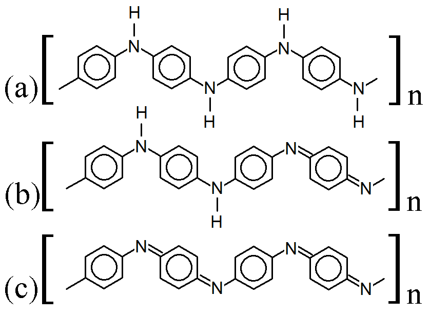
Figure 1: Lewis structures of PANIs. (a) leucoemeraldine, (b) emeraldine, and (c) pernigraniline drawn with ChemPlot. Cihan Sorkun et al. (2022)

Experimental studies related to PANIs and their derivatives are the primary source of information on their structural, physical, and chemical characteristics. Genies et al. (1990); Quillard et al. (1994); Bhadra and Khastgir (2008) This includes, among other things, chemical, electrochemical and gas-phase preparations, redox and polymerization mechanisms, and examinations of chemical, physical, electrochemical properties, and molecular structures. Shacklette et al. (1988); Moon and Park (1998); Genies et al. (1990) Further modifications and tuning of PANI-based materials with desired properties could greatly benefit from reliable quantum chemical predictions. Unfortunately, such studies are limited due to computational difficulties. It is well-known that such systems bear a non-negligible amount of multi-reference character, but their molecular size prohibits standard multi-configurational methods. Despite that, several attempts have been made to model the electronic structures of PANIs using quantum chemistry. One of the earliest applications is a quantum-chemical prediction of optical absorption spectra of some model PANI compounds using the intermediate neglect of differential overlap (INDO) model combined with the configuration interaction (CI) approach. Sjögren and Stafström (1988) The authors were among the first to notice the importance of the torsion angle between the quinoid rings and the C-N-C backbone. Semi-empirical methods were also used to study the hydration, stacking, and solvent effects of PANIs. de Oliveira Jr and Dos Santos (2000); Zhekova et al. (2007) Moreover, simplified model systems of PANI were studied using Density Functional Approximations (DFAs). Jansen et al. (1999); Foreman and Monkman (2003) The Hartree–Fock (HF) and DFA optimized structures of PANIs at different oxidation states and unit lengths were investigated by Lim et al., Lim et al. (2000) Mishra et al., Mishra and Tandon (2009) and Romanova et al. Romanova et al. (2010) The aforementioned studies point to an HF failure, incorrectly distributing conjugation along the polymer chain and contradicting the X-ray experimental findings. Shacklette et al. (1988) The use of DFAs improves the theoretical results concerning experimental structures. However, the resulting properties strongly depend on the choice of the exchange–correlation (xc) functional. Mishra and Tandom Mishra and Tandon (2009) used DFAs to investigate the infrared (IR) and Raman spectra of LB and its oligomers. Zhang et al.. Zhang et al. (2017) studied electronically excited states of model PANI complexes with water using time-dependent DF Theory (TD-DFT).

In this work, we reexamine the electronic structures and properties of PANIs using various approximations to the xc functional and unconventional electron correlation methods based on the pair Coupled Cluster Doubles (pCCD) model, Limacher et al. (2013); Stein et al. (2014); Tecmer and Boguslawski (2022, 2022) initially introduced as the Antisymmetric Product of 1-reference orbital Geminal (AP1roG) ansatz. Limacher et al. (2013) An additional advantage of pCCD-based methods is the possibility to optimize all orbitals at the correlated level and a quantitative description of orbital-based correlations using concepts from quantum information theory. K. Boguslawski, P. Tecmer (2017); Boguslawski and Tecmer (2015) The pCCD model combined with an orbital optimization protocol Boguslawski et al. (2014, 2014, 2014) proved to be a reliable tool for modeling complex electronic structures and potential energy surfaces featuring strong correlation. Tecmer et al. (2014); Boguslawski et al. (2014); Tecmer et al. (2015, 2019) Extensions to excited states within the Equation of Motion (EOM) formalism Rowe (1968); Stanton and Bartlett (1993) allow us to model double electron excitations, Boguslawski (2016, 2017, 2019) a known struggle for standard EOM-CCSD-based approaches. Watts and Bartlett (1994) All these features are desired in quantum chemical descriptions of electronic structures and properties of conducting polymers. Thus, pCCD-based quantum chemistry methods are promising alternatives to DFAs which might significantly speed up the structure-to-properties search in organic electronics and guide the experimental synthesis of new conductive polymers.

This work is organized as follows. Section II summarizes the computational methodology. Section III scrutinizes the ground- and electronic excited-states properties of selected PANIs combined with a quantum information analysis of orbital correlations. We conclude in Section IV.

II Computational details

II.1 DFT calculations

All structure optimizations and vibrational frequency calculations were performed with the Turbomole6.6 Ahlrichs et al. (1989); tur software package using the PB86 Perdew (1986); Becke (1988) xc functional and the def2-TZVP basis set. F. Weigend, R. Ahlrichs (2005); Weigend (1998) The optimized xyz structures are provided in Tables S1–S7 of the ESI${\dagger}$. These structures were later used for the calculation of electronic excitation energies within the TD-DFT Runge and Gross (1984); Van Gisbergen et al. (1999) framework using the Amsterdam Density Functional (v.2018) program package, te Velde et al. (2001); adf (2018) the BP86, Perdew (1986); Becke (1988) PBE, Perdew et al. (1996) PBE0, Adamo and Barone (1999) and CAM-B3LYP Yanai et al. (2004) xc functionals, and the Triple-$\zeta$ Polarization (TZ2P) basis set. van Lenthe and Baerends (2003)

II.2 pCCD-based methods

All pCCD Tecmer and Boguslawski (2022); Limacher et al. (2013); Boguslawski et al. (2014); Stein et al. (2014) calculations were carried out in a developer version of the PyBEST software package Boguslawski et al. (2021, ) using the cc-pVDZ basis set Dunning Jr. (1989) and the DFT optimized structures. For the ground-state pCCD calculations, we employed the variational orbital optimization protocol. Boguslawski et al. (2014, 2014, 2014) The Pipek–Mezey localized orbitals Pipek and Mezey (1989) were used as a starting point for orbital optimization. Our numerical experience showed that using localized orbitals accelerates the orbital optimization process as the final pCCD natural orbitals are typically localized and bear some resemblance with split-localized orbitals. Bytautas et al. (2003)

II.2.1 Entanglement and correlation measures

The 1- and 2-reduced density matrices K. Boguslawski, P. Tecmer (2015, 2017); Boguslawski et al. (2013); Nowak et al. (2021) from variationally optimized pCCD wavefunctions were used to calculate the single orbital entropy and orbital-pair mutual information. Rissler et al. (2006); Szalay et al. (2015); Barcza et al. (2011); Ding et al. (2020) The single-orbital entropies $s_{i}$ are calculated as Rissler et al. (2006)

$$s_{i}=-\sum_{\alpha=1}^{4}\omega_{\alpha,i}\ln\omega_{\alpha,i},$$ (2)

where $\omega_{\alpha,i}$ are the eigenvalues of the one-orbital reduced density matrix, $\rho_{i,i^{\prime}}^{(1)}$, of orbital $i$. Rissler et al. (2006); Boguslawski et al. (2013); K. Boguslawski, P. Tecmer (2015, 2017) In the case of pCCD, such a one-orbital reduced density matrix (RDM) is determined from 1- and 2-particle RDMs.Boguslawski et al. (2016); Nowak et al. (2021) The (orbital-pair) mutual information $I_{i|j}$ is expressed as the difference between the amount of quantum information encoded in the two one-orbital reduced density matrices $i$ and $j$ and the two-orbital reduced density matrix associated with those two orbitals (the orbital pair $i,j$) Rissler et al. (2006)

$$I_{i|j}=s_{i}+s_{j}+\sum_{\alpha=1}^{16}\omega_{\alpha,i,j}\mathrm{ln}\omega_{\alpha,i,j}.$$ (3)

where $\omega_{\alpha,i,j}$ stands for the eigenvalues of the two-orbital RDM. Its matrix elements can be determined by generalizing the two-orbital analog of $\rho_{i,i^{\prime}}^{(1)}$. Boguslawski et al. (2013); K. Boguslawski, P. Tecmer (2015, 2017); Szalay et al. (2015); Boguslawski et al. (2016); Nowak et al. (2021)

II.2.2 Electronic excitation energies

The vertical electronic excitation energies were calculated using the CIS, EOM-pCCD, EOM-pCCD+S, and EOM-pCCD-CCS methods Boguslawski (2016, 2017); Nowak and Boguslawski (2023) available in PyBEST. Boguslawski et al. (2021, ) While in the EOM-pCCD approach, only electron-pair excitations are present in the linear excitation operator, EOM-pCCD+S and EOM-pCCD-CCS also include single excitations (see refs. 47; 48 for more details). Thus, with the EOM-pCCD model, only electron-pair excitations are computed, while the EOM-pCCD+S and EOM-pCCD-CCS models allow us to determine single and double electron excitations. All EOM-pCCD+S calculations used the ground-state orbital-optimized pCCD reference, and all others the canonical HF orbitals.

III Results and discussion

In the following, we discuss the structural, vibrational, and electronically excited-state parameters of the aniline binary compound and selected PANIs in their tetramer and octamer structural arrangements. The results are compared to experiments and other theoretical predictions. Furthermore, the TD-DFT excitation energies obtained from different xc functionals are compared to wave-function calculations. Finally, we use an orbital entanglement and correlation analysis of orbital interactions for assessing the electronic structures and changes in electron correlation effects in PANIs of various oxidation states and lengths.

Table 1: BP86 optimized structural parameters of PANI. Lewis structures are depicted in Figure 3, atomic labels correspond to those in Figures S1 and S2 of the ESI†.

1t		1o
Geometrical parameters	Bond length [Å]	Geometrical parameters	Bond length [Å]
N7-C4, N7-C8	1.393, 1.406	N58-C55, N58-C59	1.393, 1.404
C4-C3, C8-C9	1.409, 1.406	C55-C54, C59-C60	1.409, 1.406
C3-C2, C9-C10	1.395, 1.390	C54-C53, C60-C61	1.395, 1.391
C2-C1, C10-C11	1.397, 1.409	C53-C52, C61-C62	1.397, 1.408
C1-C6, C11-C12	1.399, 1.407	C52-C57, C62-C63	1.399, 1.408
C6-C5, C12-C13	1.392, 1.393	C57-C56, C63-C64	1.392, 1.392
C5-C4, C13-C8	1.411, 1.405	C56-C55, C64-C59	1.411, 1.406
Geometrical parameters	Bond angle [∘]	Geometrical parameters	Bond angle [∘]
C4-N7-C8	129.1	C55-N58-C59	129.4
N7-C4-C3	123.1	N58-C55-C54	123.0
N7-C8-C9	122.8	N58-C59-C60	123.1
Geometrical parameters	Dihedral angle [∘]	Geometrical parameters	Dihedral angle [∘]
C8-N7-C4-C3	15.1	C59-N58-C55-C54	22.6
C4-N7-C8-C9	36.3	C55-N58-C59-C60	28.1
2t		2o
Geometrical parameters	Bond length [Å]	Geometrical parameters	Bond length [Å]
N7-C4, N7-C8	1.398, 1.394	N58-C55, N58-C59	1.397, 1.399
C4-C3, C8-C9	1.408, 1.411	C55-C54, C59-C60	1.408, 1.407
C3-C2, C9-C10	1.395, 1.386	C54-C53, C60-C61	1.395, 1.391
C2-C1, C10-C11	1.397, 1.416	C53-C52, C61-C62	1.397, 1.407
C1-C6, C11-C12	1.398, 1.419	C52-C57, C62-C63	1.398, 1.406
C6-C5, C12-C13	1.392, 1.387	C57-C56, C63-C64	1.392, 1.391
C5-C4, C13-C8	1.409, 1.411	C56-C55, C64-C59	1.410, 1.408
Geometrical parameters	Bond angle [∘]	Geometrical parameters	Bond angle [∘]
C4-N7-C8	129.9	C55-N58-C59	129.6
N7-C4-C3	122.9	N58-C55-C54	123.1
N7-C8-C9	123.3	N58-C59-C60	123.1
Geometrical parameters	Dihedral angle [∘]	Geometrical parameters	Dihedral angle [∘]
C8-N7-C4-C3	25.5	C59-N58-C55-C54	19.5
C4-N7-C8-C9	22.2	C55-N58-C59-C60	29.7
3t		3o
Geometrical parameters	Bond length [Å]	Geometrical parameters	Bond length [Å]
N7-C4, N7-C8	1.389, 1.313	N58-C55, N58-C59	1.388, 1.314
C4-C3, C8-C9	1.414, 1.457	C55-C54, C59-C60	1.415, 1.457
C3-C2, C9-C10	1.394, 1.357	C54-C53, C60-C61	1.394, 1.358
C2-C1, C10-C11	1.398, 1.454	C53-C52, C61-C62	1.398, 1.453
C1-C6, C11-C12	1.400, 1.456	C52-C57, C62-C63	1.400, 1.455
C6-C5, C12-C13	1.391, 1.357	C57-C56, C63-C64	1.391, 1.358
C5-C4, C13-C8	1.413, 1.455	C56-C55, C64-C59	1.413, 1.455
Geometrical parameters	Bond angle [∘]	Geometrical parameters	Bond angle [∘]
C4-N7-C8	123.4	C55-N58-C59	123.4
N7-C4-C3	123.4	N58-C55-C54	123.4
N7-C8-C9	123.4	N58-C59-C60	126.4
Geometrical parameters	Dihedral angle [∘]	Geometrical parameters	Dihedral angle [∘]
C8-N7-C4-C3	48.1	C59-N58-C55-C54	47.4
C4-N7-C8-C9	10.7	C55-N58-C59-C60	11.1

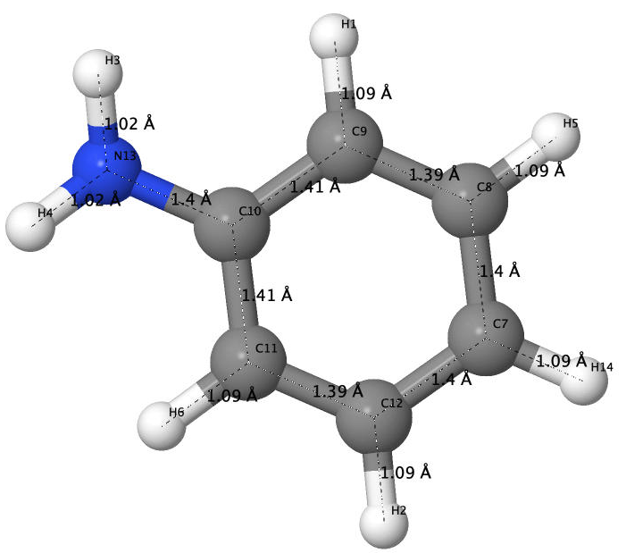
Figure 2: DFT-optimized structure of aniline including bond lengths in Å.

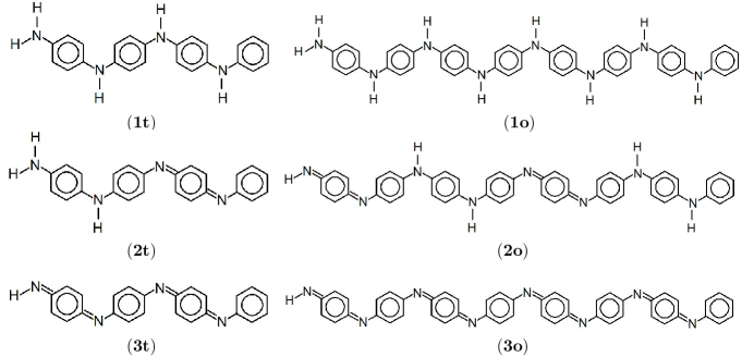
Figure 3: Lewis structures of polyanilies drawn with ChemPlot Cihan Sorkun et al. (2022). Subfigures display leucoemeraldine (1), emeraldine (2), and pernigraniline (3) in the tetramer (t) and octamer (o) forms.

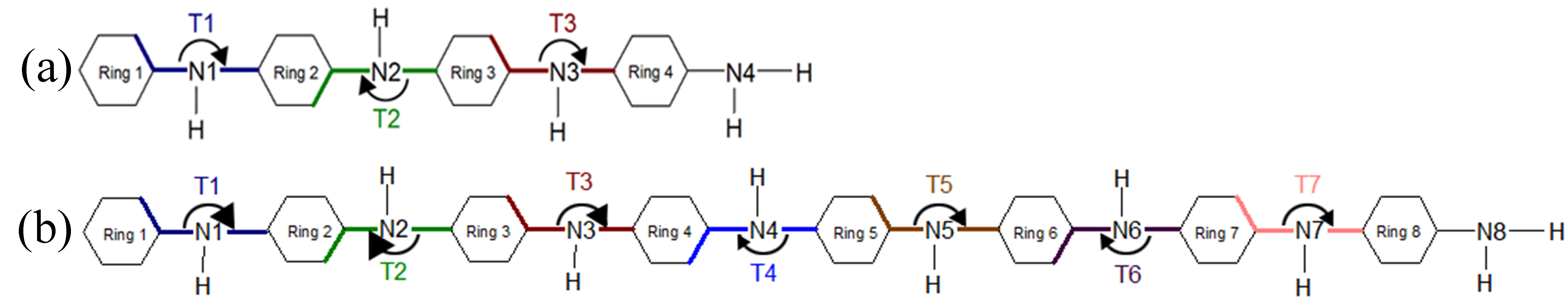
Figure 4: Schematic representation of the T1–T7 ring tilt angles in the tetramer (a) and octamer (b) models of PANIs.

Table 2: The ring tilt angles T1–T7 [^∘] as labeled in Figure 4 of the tetramer (t) and octamer (o) forms of PANIs optimized with BP86/def2-TZVP.

	1t	1o	2t	2o	3t	3o
T1	166.6	159.7	157.2	162.8	137.6	138.4
T2	194.9	206.3	212.9	204.7	191.7	192.7
T3	165.0	159.0	168.3	148.7	141.9	146.1
T4		201.9		192.4		194.3
T5		156.3		158.0		146.9
T6		205.2		206.4		193.5
T7		158.8		149.2		142.6

III.1 Ground-state optimized electronic structures

The optimized structure of aniline, a small building block of PANIs, is shown in Figure 2. All optimized bond lengths between N-H are roughly equal to 1.016 Å, while the C-H bond length equals 1.09 Å. The optimized structures of leucoemeraldine (1t), emeraldine (2t), and pernigraniline (3t) in the tetramer form and in their corresponding octamer forms (1o, 2o, and 3o) are visualized in Figures S1 and S2 of the ESI†, respectively. Figure 3 shows the corresponding Lewis structures, highlighting that aniline is a building block of PANIs. Our DFT calculations predict C-C and C-N bond distances between 1.3 and 1.4 Å (see Table 1). The bond angle between two phenyl rings in 1t and 1o and 2t and 2o is almost the same and averages to 125^∘. In contrast, the dihedral angles between the rings feature an average value of around 26.33^∘. For 3t and 3o, the bond angle between the two phenyl rings is pretty similar except for the angle $\ce{N}58\ce{-C}59\ce{-C}60$, which increases to 126.4^∘. The dihedral angles of 3t and 3o significantly grow to 48.1^∘ and 47.4^∘, respectively, compared to 1t and 1o. The total torsion angle between the phenyl rings is one of the main factors that govern the band gaps, conjugation length, and electrical conductivity, all of which are important factors in determining the electronic properties of PANIs. For this purpose, we collected the tilt angles (as indicated in Figure 4 and collected in Table 2) for all the tetramer (t) and octamer (o) forms of the investigated PANIs. Our data suggest that the tilt angle for 3t and 3o significantly decreases compared to the remaining PANI compounds. That coincides with the theoretically best conductive properties of 3t and 3o over the remaining PANIs at lower oxidation states.

Table 3: Experimental and BP86 vibrational frequencies $[$cm${}^{-1}]$ for aniline and all investigated PANIs.

Molecule	Exp.Quillard et al. (1994)	This work
		Freq. $[$cm${}^{-1}]$	Intensity $[$km/mol$]$	Assignment
Aniline	1620	1612	153.261	N-H2 bending
	1603	1580	4.343	C-C ring stretching
	1276	1276	53.756	C-N stretching
	1176, 1155	1147	1.333	C-H bending
		Tetramer (t)
1t	1618	1621	13.936	C-C ring stretching
		1616	18.881	C-C ring stretching
		1615	26.274	C-C ring stretching
		1599	206.853	C-C ring stretching
		1602	62.197	N-H2 bending
	1219	1221	15.378	C-N stretching
		1219	6.463	C-N stretching
	1181	1165	4.293	C-H bending
		1163	0.161	C-H bending
2t	1617	1619	91.950	C-C ring stretching
		1606	506.207	N-H2 bending
	1519	1519	254.253	C=N stretching
	1220, 1219	1227	6.510	C-N stretching
		1222	3.694	C-N stretching
	1182	1168	2.785	C-H bending
		1155	132.108	C-H bending
		1153	150.552	C-H bending
		1144	1.584	C-H bending
3t	1612, 1553	1556	49.940	C-C ring stretching
	1582, 1579	1588	2.021	C=C stretching
		1581	5.799	C=C stretching
	1480	1496	77.580	C=N stretching
	1219	1235	0.642	C-N stretching
		1229	7.934	C-N stretching
		1218	22.962	C-N stretching
	1157	1157	2.481	C-H bending
		Octamer (o)
1o	1618	1622	5.474	C-C ring stretching
		1617	0.271	C-C ring stretching
		1616	5.865	C-C ring stretching
		1615	16.793	C-C ring stretching
		1599	206.640	C-C ring stretching
		1602	70.742	N-H2 bending
	1219	1221	1.003	C-N stretching
		1220	7.350	C-N stretching
		1219	41.414	C-N stretching
	1181	1165	6.165	C-H bending
		1164	0.405	C-H bending
		1163	1.103	C-H bending
2o	1617	1616	23.481	C-C ring stretching
	1519	1515	169.019	C=N stretching
	1220, 1219	1224	45.260	C-N stretching
		1223	21.564	C-N stretching
		1221	4.281	C-N stretching
	1182	1169	1.030	C-H bending
		1166	3.486	C-H bending
		1165	76.322	C-H bending
		1157	113.823	C-H bending
		1155	455.013	C-H bending
		1149	0.902	C-H bending
		1143	21.476	C-H bending
3o	1612, 1553	1586	8.260	C-C ring stretching
		1581	5.022	C-C ring stretching
	1582, 1579	1589	5.578	C=C stretching
		1574	7.336	C=C stretching
	1480	1490	158.490	C=N stretching
		1472	0.771	C=N stretching
	1219	1218	53.816	C-N stretching
	1157	1157	8.286	C-H bending
		1148	269.192	C-H bending

III.2 Vibrational spectra

Aniline and PANIs have been a significant target of structural and electronic studies, experimentally and theoretically, for many years Piest et al. (1999); Wojciechowski et al. (2003); Quillard et al. (1994); Lim et al. (2000); Mishra (2015); Mishra and Tandon (2009). Table 3 presents a complete vibrational assignment of all fundamental vibrations and a comparison to experimental data. Quillard et al. (1994) Most importantly, all theoretical data agrees with experimental results for aniline and PANIs. The vibrational spectra of all investigated PANIs are reconstructed in Figure S3 of the ESI† using the Gabedit software package. In the spectrum of aniline, two peaks appear at 1612 and 1580 cm^-1. The former is assigned to the $\ce{-N}\ce{H}2$ bending and the latter to the $\ce{C}\ce{-C}$ ring-stretching vibration of the phenyl group. The remaining leading vibrations of the Raman and IR spectra are located at 1276 cm^-1 and correspond to the ring-stretching mode mainly attributed to the $\ce{C}\ce{-N}$ stretching. The band at 1147 cm^-1 results from the $\ce{C}\ce{-H}$ bending mode. All the characteristic features of the aniline vibrational spectrum are present in all investigated PANIs, except for the -NH2 peak that is absent in 3t and 3o.

For 1t we observe several characteristic vibrations of the benzene ring, such as those peaked at 1599, 1615, 1616, and 1621 cm^-1, which correspond to a $\ce{C}\ce{-C}$ stretching vibrational mode for ring 1, 2, 3, and 4, respectively, (cf. Figure 4 for ring labels) and two $\ce{C}\ce{-H}$ bending vibrational modes at 1165 and 1163 cm^-1. The bands at 1221, and 1219 cm^-1 correspond to the $\ce{C}\ce{-N}$ stretching vibrational mode for $\ce{N}1$, $\ce{N}2$, and $\ce{N}3$ respectively, while the $\ce{-N}\ce{H2}$ bending mode is positioned at 1602 cm^-1 (the atomic labels are indicated in Figure S1 of the ESI†).

For 2t, the $\ce{C}\ce{-C}$ ring-stretching is located at 1619 cm^-1, and the $\ce{C}\ce{=N}$ stretching mode at 1519 cm^-1. The two peaks at 1222 ($\ce{N}1$) and 1227 ($\ce{N}2$ and $\ce{N}3$) cm^-1 are due to a $\ce{C}\ce{-N}$ stretching mode (see also Figure S1 of the ESI† for atomic labels). The $\ce{C}\ce{-H}$ bending vibrational mode of the benzene ring can be characterized by a Raman band at 1168, 1155, 1153, and 1144 cm^-1, respectively. The $\ce{-N}\ce{H2}$ bending mode is positioned at 1606 cm^-1.

3t features the fundamental bands of $\ce{C}\ce{=C}$ stretching modes at 1581 and 1588 cm^-1 and a $\ce{C}\ce{-C}$ ring-stretching mode at 1556 cm^-1. The Raman band at 1496 cm^-1 corresponds to a $\ce{C}\ce{=N}$ stretching vibrational mode, while the $\ce{C}\ce{-N}$ stretching mode is positioned at 1217, 1228, and 1234 cm^-1. The $\ce{C}\ce{-H}$ bending mode is predicted at 1157 cm^-1.

Comparing the characteristic vibrational features of 1t, 2t, and 3t, we note a redshift of the C-C ring stretching and C-H bending frequencies. Moreover, we observe a blueshift of the N-H2 bending vibrations from 1t to 2t. Essentially the same vibrational features as for 1t, 2t, and 3t are observed for 1o, 2o, and 3o, respectively. The only difference is the larger number of peaks and a negligible increase in characteristic vibrational frequencies by about 1-2 cm^-1 for longer polymer chains (cf. Table 3).

III.3 HOMO–LUMO gaps from DFAs

The HOMO and LUMO molecular orbitals of 1t, 2t, 3t, 1o, 2o, and 3o  obtained from different xc functionals (BP86, PBE, PBE0, and CAM-B3LYP) are depicted in Figures S5-S8 of the ESI†. All xc functionals predict similar HOMO and LUMO $\pi$- and $\pi^{*}$-type molecular orbitals delocalized over the whole molecular structures. The HOMO and LUMO energies and the HOMO–LUMO gaps are summarized in Table S8 and visualized in Figure S4 of the ESI†. Both generalized gradient approximations to the xc functional (BP86 and PBE) predict identical HOMO–LUMO gaps for aniline and almost identical for all PANIs. The PBE0 xc functional with an admixture of 25${\%}$ of HF exchange roughly doubles the HOMO–LUMO gaps. The range-separated CAM-B3LYP xc functional further widens the HOMO–LUMO gaps by about 20-25${\%}$. Specifically, CAM-B3LYP predicts the HOMO–LUMO gap of 0.29 eV for aniline, and 0.196 eV for 1t, 0.155 eV for 2t, and 0.162 eV for 3t, respectively. The HOMO–LUMO gap is only slightly affected (lowered by around 0.01 eV) in the longer PANIs (1o, 2o, and 3o). Finally, we should note that our DFA calculations do not show any clear trend of the HOMO–LUMO gap with respect to the formal oxidation state of PANIs.

Table 4: Lowest-lying singlet–singlet excitation energies [eV] and their characteristics calculated from TD-DFT, EOM-pCCD+S, and CIS. HOMO and LUMO are abbreviated as H and L, respectively. Note that EOM-pCCD+S was performed using the natural pCCD orbitals, which are ordered with respect to occupation numbers, not orbital energies.

Molecule	no.	character	PB86	PBE	PBE0	CAM-B3LYP	EOM-pCCD+S	CIS
Aniline		energy	4.422	4.410	4.820	4.912	6.005	5.821
		weight	0.900	0.900	0.880	0.860	0.485	0.618
	1	character	H$\rightarrow$ L	H$\rightarrow$ L	H$\rightarrow$ L	H$\rightarrow$ L	H-1$\rightarrow$ L	H$\rightarrow$ L
		intensity	0.029	0.029	0.038	0.040	–	–
		energy	4.903	4.660	5.180	5.253	6.880	6.174
		weight	0.850	0.810	0.550	0.950	0.445	0.551
	2	character	H$\rightarrow$ L+2	H$\rightarrow$ L+2	H$\rightarrow$ L+2	H$\rightarrow$ L+1	H-1$\rightarrow$ L+1	H$\rightarrow$ L+1
		intensity	0.013	0.008	0.013	0.012	–	–
		energy	5.373	5.250	5.670	5.737	8.002	7.304
		weight	0.660	0.820	0.430	0.810	0.309	0.578
	3	character	H$\rightarrow$ L+1	H$\rightarrow$ L+3	H$\rightarrow$ L+1	H$\rightarrow$ L+2	H-11$\rightarrow$ L+3	H$\rightarrow$ L+2
		intensity	0.131	0.024	0.130	0.128	–	–
1t		energy	2.791	2.780	3.547	3.916	5.525	4.913
		weight	0.570	0.490	0.720	0.600	0.192	0.552
	1	character	H$\rightarrow$ L	H$\rightarrow$ L	H$\rightarrow$ L	H$\rightarrow$ L	H-38$\rightarrow$ L+3	H$\rightarrow$ L
		intensity	0.027	0.025	0.562	0.839	–	–
		energy	2.834	2.823	3.632	4.000	5.645	5.116
		weight	0.720	0.770	0.690	0.530	0.231	0.534
	2	character	H$\rightarrow$ L+2	H$\rightarrow$ L+2	H$\rightarrow$ L+1	H$\rightarrow$ L+1	H-32$\rightarrow$ L+3	H$\rightarrow$ L+1
		intensity	0.036	0.035	0.724	0.558	–
		energy	2.918	2.894	3.700	4.092	5.692	5.220
		weight	0.440	0.430	0.880	0.600	0.293	0.484
	3	character	H$\rightarrow$ L+1	H$\rightarrow$ L+1	H$\rightarrow$ L+2	H$\rightarrow$ L+2	H-33$\rightarrow$ L+1	H$\rightarrow$ L+2
		intensity	0.647	0.671	0.033	0.032	–	–
2t		energy	1.734	1.729	2.078	2.376	4.381	3.173
		weight	0.880	0.880	0.940	0.890	0.212	0.628
	1	character	H$\rightarrow$ L	H$\rightarrow$ L	H$\rightarrow$ L	H$\rightarrow$ L	H-43$\rightarrow$ L+1	H$\rightarrow$ L
		intensity	0.912	0.909	1.177	1.301	–	–
		energy	2.012	2.001	2.429	2.814	4.987	3.872
		weight	0.890	0.890	0.890	0.740	0.332	0.509
	2	character	H-1$\rightarrow$ L	H-1$\rightarrow$ L	H-1$\rightarrow$ L	H-1$\rightarrow$ L	H-42$\rightarrow$ L	H-1$\rightarrow$ L
		intensity	0.091	0.087	0.022	0.001	–	–
		energy	2.583	2.573	3.304	3.896	5.821	4.972
		weight	0.890	0.900	0.610	0.190	0.312	0.429
	3	character	H-2$\rightarrow$ L	H-2$\rightarrow$ L	H-2$\rightarrow$ L	H-4$\rightarrow$ L	H-28$\rightarrow$ L+6	H-9$\rightarrow$ L
		intensity	0.001	0.001	0.021	0.674	–	–
3t		energy	1.676	1.671	2.087	2.413	4.468	3.216
		weight	0.580	0.580	0.940	0.870	0.255	0.617
	1	character	H$\rightarrow$ L	H$\rightarrow$ L	H$\rightarrow$ L	H$\rightarrow$ L	H-45$\rightarrow$ L+2	H$\rightarrow$ L
		intensity	0.566	0.564	1.198	1.327	–	–
		energy	1.770	1.763	2.450	2.916	5.123	3.923
		weight	0.380	0.370	0.500	0.440	0.384	0.405
	2	character	H$\rightarrow$ L	H$\rightarrow$ L	H$\rightarrow$ L+1	H-1$\rightarrow$ L	H-46$\rightarrow$ L+1	H-1$\rightarrow$ L
		intensity	0.378	0.367	0.010	0.025	–	–
		energy	2.012	2.002	2.539	2.942	5.284	4.049
		weight	0.540	0.560	0.440	0.430	0.382	0.343
	3	character	H$\rightarrow$ L+1	H$\rightarrow$ L+1	H$\rightarrow$ L+1	H$\rightarrow$ L+1	H-45$\rightarrow$ L+2	H$\rightarrow$ L+1
		intensity	0.005	0.005	0.011	0.021	–	–
1o		energy	2.381	2.364	3.266	∗–	5.349	4.683
		weight	0.900	0.900	0.670	∗–	0.111	0.408
	1	character	H$\rightarrow$ L	H$\rightarrow$ L	H$\rightarrow$ L	∗–	H-78$\rightarrow$ L+9	H$\rightarrow$ L
		intensity	0.375	0.397	2.618	∗–	–	–
		energy	2.473	2.456	3.470	∗–	5.516	4.899
		weight	0.870	0.900	0.280	∗–	0.165	0.342
	2	character	H$\rightarrow$ L+1	H$\rightarrow$ L+1	H$\rightarrow$ L+4	∗–	H-53$\rightarrow$ L+6	H-1$\rightarrow$ L
		intensity	0.085	0.061	0.111	∗–	–	–
		energy	2.535	2.523	3.486	∗–	5.548	5.043
		weight	0.570	0.530	0.370	∗–	0.179	0.267
	3	character	H$\rightarrow$ L+2	H$\rightarrow$ L+2	H$\rightarrow$ L+3	∗–	H-52$\rightarrow$ L+3	H$\rightarrow$ L+2
		intensity	0.007	0.009	0.253	∗–	–	–
2o		energy	0.970	0.970	1.783	∗–	4.249	3.042
		weight	0.780	0.770	0.940	∗–	0.204	0.559
	1	character	H$\rightarrow$ L	H$\rightarrow$ L	H$\rightarrow$ L	∗–	H-85$\rightarrow$ L+1	H$\rightarrow$ L
		intensity	0.150	0.152	2.217	∗–	–	–
		energy	1.272	1.268	1.996	∗–	4.675	3.548
		weight	0.410	0.400	0.950	∗–	0.329	0.374
	2	character	H$\rightarrow$ L+1	H$\rightarrow$ L+1	H$\rightarrow$ L+1	∗–	H-84$\rightarrow$ L+2	H-1$\rightarrow$ L+1
		intensity	1.379	1.386	0.002	∗–	–	–
		energy	1.347	1.345	2.088	∗–	4.896	3.792
		weight	0.290	0.290	0.910	∗–	0.310	0.326
	3	character	H-1$\rightarrow$ L	H-1$\rightarrow$ L	H-1$\rightarrow$ L	∗–	H-86$\rightarrow$ L+3	H-3$\rightarrow$ L
		intensity	0.013	0.010	0.004	∗–	–	–
3o		energy	1.093	1.090	1.524	∗–	3.959	2.598
		weight	0.480	0.480	0.930	∗–	0.159	0.558
	1	character	H$\rightarrow$ L+1	H$\rightarrow$ L+1	H$\rightarrow$ L	∗–	H-3$\rightarrow$ L+3	H$\rightarrow$ L
		intensity	0.090	0.069	3.561	∗–	–	–
		energy	1.117	1.114	1.893	∗–	4.370	3.135
		weight	0.810	0.810	0.480	∗–	0.174	0.408
	2	character	H$\rightarrow$ L	H$\rightarrow$ L	H-1$\rightarrow$ L	∗–	H-81$\rightarrow$ L+4	H-1$\rightarrow$ L
		intensity	1.970	1.976	0.000	∗–	–	–
		energy	1.349	1.344	2.028	∗–	4.679	3.524
		weight	0.550	0.560	0.490	∗–	0.216	0.382
	3	character	H-2$\rightarrow$ L	H-2$\rightarrow$ L	H$\rightarrow$ L+1	∗–	H-84$\rightarrow$ L+3	H-2$\rightarrow$ L
		intensity	0.003	0.009	0.000	∗–	–	–

• ^∗ The CAM-B3LYP ground-state calculations for 1o, 2o, and 3o did not converge due to numerical difficulties.

III.4 Electronic excitation energies

A significant feature of conjugated polymers often studied theoretically and experimentally is the electronic structure of their valence band. The desired donor properties feature high-intensity electronic transitions with a dominant HOMO $\rightarrow$ LUMO character in the specific range of the spectrum. Cui et al. (2020) Therefore, we will scrutinize the lowest-lying electronic excitation energies obtained from different quantum chemistry methods to assess the structure-to-property relationship. Table 4 summarizes low-lying electronic transition energies and associated characteristics obtained from various xc functionals (BP86, PBE, PBE0, and CAM-B3LYP), CIS, and EOM-pCCD+S. The EOM-pCCD and EOM-pCCD-CCS excitation energies are reported in Table S9 of the ESI† for comparison.

III.4.1 TD-DFT and CIS excitation energies

The HOMO $\rightarrow$ LUMO excitations dominate the first excitation energy in TD-DFT studies of all investigated molecules and have non-zero transition dipole moments (TDMs). The higher-lying excitations involve mainly an electron transfer from HOMO to LUMO+1 and LUMO+2 orbitals, with the latter having $\pi^{*}$ character. An exception is 2, for which the second and third excited states occur from $\pi$-type orbitals lower than the HOMO. Thus, the low-lying part of the electronic spectrum of PANIs is dominated by $\pi\rightarrow\pi^{*}$ transitions. PANIs significantly lower the electronic transitions observed in the aniline model system. Specifically, they fall in an energetic descending order 1t ¡ 1o ¡ 3t ¡ 3o ¡ 2t ¡ 2o, indicating that emeraldine has the lowest-lying electronic transitions among them all. Genies et al. (1990) This observation aligns with the common knowledge about the best conductive properties of emeraldine. Yet, moving from structures t to o, we observe a lowering of excitations by about 0.3-0.4 eV. We should also stress that the HOMO/LUMO orbital energies and the HOMO-LUMO gaps discussed in the previous subsection do not correlate with the low-lying electronic spectrum of PANIs.

The absolute values of excitation energies and, to some extent, their characteristics strongly depend on the applied xc functional. Based on previous TD-DFT benchmarks and analysis of excitation energies, we do not expect any outstanding performance from semi-local xc functionals like BP86 and PBE, as they tend to underestimate electron excitations. Dreuw and Head-Gordon (2005); Laurent and Jacquemin (2013); Körzdörfer and Brédas (2014) Adding HF exchange to the xc functional should improve the overall performance as we include non-local effects in the xc kernel. We expect further enhancement of the description of charge-transfer states with range-separated hybrids. Dreuw et al. (2003); Dreuw and Head-Gordon (2004); Tecmer et al. (2011, 2012, 2013) Thus, we anticipate the PBE0 and CAM-B3LYP results to be more reliable, although limited to model single electronic transitions and electronic structures well-described by a single Slater determinant. The difference between the PBE0 and CAM-B3LYP excitation energies can be used to identify possible charge-transfer states. Based on that, we anticipate that all investigated PANI structures have some admixture of charge-transfer character, with aniline being the exception. The nature of PBE0 and CAM-B3LYP transitions is very similar, except for structure 1t, where the order of the 2-nd and 3-rd excited state changes. The PBE0 and CAM-B3LYP excitation energies are comparable in magnitude to the CIS data: electronic transitions’ order and main character are virtually the same. They differ, however, in the absolute values of excitation energies (cf. Table 4), where CIS predicts higher excitation energies. The most considerable discrepancies are observed for the aniline molecule (up to 1.5 eV) and are further reduced to approximately 1 eV in PANIs.

III.4.2 EOM-pCCD+S excitation energies

The EOM-pCCD+S excitation energies are comparable, indicating dominant contributions from single electronic excitations. The double electronic transitions are in the upper spectrum, as shown in Table S9 of the ESI†. The significant difference between the EOM-pCCD+S and CIS methods originates from the orbital bases: EOM-pCCD+S utilized the pCCD-optimized orbitals that are localized in nature (see Figures S10-S18 of the ESI†), while CIS used the canonical HF orbitals (delocalized). Thus, the pCCD-optimized orbitals offer a different viewpoint, in which the information is more compressed and often easier to interpret. Ben Amor et al. (2021); Stewart (2019) We should also note that the pCCD orbitals are sorted according to their (natural) occupation numbers, whose order does not correspond to the energetic order of the canonical HF orbitals. Unlike TD-DFT and CIS, where the electronic transitions are dominated by one main electronic configuration, each electronic transition in EOM-pCCD+S includes several orbital contributions of similar weights but often of various characteristics (the pCCD orbitals involved in the low-lying excitations are shown in Figures S10-S18 of the ESI†). The local nature of pCCD orbitals, thus, allows us to dissect the character of each transition in PANIs and their structure-to-property relationship.

For 1t, all three lowest excitations have leading contributions from the $\pi_{\rm B}\rightarrow\pi_{\rm B}^{*}$, where B indicates the benzenoid rings. They differ between themselves in the admixture of transitions from the nitrogen lone pair (LP) orbital to the $\pi_{\rm B}^{*}$ and $\sigma^{*}$ orbitals. In the second and third excited state of 1t, transitions of the $\pi_{\rm B}\rightarrow\sigma^{*}$ character appear additionally. Upon polymer elongation (1o), the excitations become almost solely dominated by the $\pi_{\rm B}\rightarrow\pi_{\rm B}^{*}$ transitions.

The electronic spectrum of 2t is very complex and involves transitions of many characters. The leading contributions for the first excited state come from the nitrogen lone-pairs (LP_N), $\pi_{\rm N}$, and $\pi_{\rm B}$ orbitals to the $\pi^{*}_{\rm N}$ orbital (where the subscript N underlines that the orbital is centered at the nitrogen atom). Additionally, we find smaller but non-negligible contributions of type $\pi_{\rm N}\rightarrow\pi^{*}_{\rm N}$, $\pi_{\rm Q}\rightarrow\pi^{*}_{\rm N}$, and $\pi_{\rm N}\rightarrow\pi^{*}_{\rm Q}$, where the index Q indicates the quinoid ring. LP$\rightarrow\pi_{N}^{*}$ and $\pi_{\rm B}\rightarrow\pi^{*}_{\rm N}$ electronic transitions dominate the second excited state and $\pi_{\rm B}\rightarrow\pi^{*}_{\rm B}$ the third excited state of 2t, respectively. Moving to 2o, we observe a more organized spectrum composed of less diverse transitions. Specifically, these are $\pi_{\rm Q}\rightarrow\pi^{*}_{\rm Q}\backslash\pi^{*}_{\rm N}$ and $\pi_{\rm B}\rightarrow\pi^{*}_{\rm Q}\backslash\pi^{*}_{\rm N}$ transitions for the first, LP$\rightarrow\pi^{*}_{\rm N}$, $\pi_{\rm Q}\rightarrow\pi^{*}_{\rm N}$, and $\pi_{\rm B}\rightarrow\pi^{*}_{\rm Q}$ transitions for the second, and the LP$\rightarrow\pi^{*}_{\rm N}$ and $\pi_{\rm B}\rightarrow\pi^{*}_{\rm N}$ transitions for the third excited state, respectively. Thus, the elongation of emeraldine (2) profoundly affects its low-lying electronic transitions, revealing the involvement of quinoid rings only in the octamer configuration.

The electronic spectrum of 3t is as complex as 2t, differing mainly in the increased involvement of quinoid orbitals and the presence of $\sigma_{N}$ orbitals (see the corresponding orbitals in Figures S10-S18 of the ESI†). The first excited state of 3t is dominated by LP$\rightarrow\pi^{*}_{\rm B}$, $\sigma_{\rm B}\rightarrow\pi^{*}_{\rm N}$, and $\pi_{\rm Q}\rightarrow\pi^{*}_{\rm Q}$ transitions, the second one by LP$\rightarrow\pi^{*}_{\rm N}$, $\sigma_{\rm B}\rightarrow\pi^{*}_{\rm B}$, and $\pi_{\rm R}\rightarrow\pi^{*}_{\rm Q}$ transitions, and the third one by LP$\rightarrow\pi^{*}_{\rm B}$, $\sigma_{\rm B}\rightarrow\pi^{*}_{\rm B}$, and $\sigma_{\rm N}\rightarrow\pi^{*}_{\rm B}$ transitions. The electronic spectrum of the corresponding structure 3o is less complex, dominated by three main types of transitions. Specifically, these are $\pi_{\rm Q}\rightarrow\pi^{*}_{\rm N}$ and LP$\rightarrow\pi^{*}_{\rm N}$ transitions for the first excited state, LP$\rightarrow\pi^{*}_{\rm N}$, $\pi_{\rm Q}\rightarrow\pi^{*}_{\rm N}$, and $\pi_{\rm B}\rightarrow\pi^{*}_{\rm N}$ transitions for the second one, and LP$\rightarrow\pi^{*}$ and $\pi_{\rm B}\rightarrow\pi^{*}_{\rm N}$ transitions for the third one, respectively.

Finally, the EOM-pCCD+S excitation energies are higher than CIS results by about 0.6 eV for 1t, 1.2 eV for 2t, 1.3 eV for 3t, 0.7 eV for 1o, 1.2 eV for 2o, and 1.4 eV for 3o and overall higher by about 1-2 eV than the PBE and CAM-B3LYP results.

III.5 Orbital-pair correlation analysis

To better understand the electronic structures and the structure-to-property relationship of the investigated PANIs, we performed an orbital-pair mutual information analysis depicted in Figure 5. The strength of the mutual information (that is, orbital-pair correlations) is color-coded in Figure 5. Furthermore, only the most strongly-correlated orbital pairs are shown for better visibility. Interestingly, all the investigated systems have the most correlated orbitals around the valence region (the benzenoid/quinoid ring). These are the $\pi$ and $\pi^{*}$ orbital combinations, including the HOMO–LUMO pairs. They do not coincide entirely with the pCCD orbitals involved in the electronic excitations. The pCCD orbitals are optimal for the ground but not necessarily for excited state structures. For aniline, we observe only two strongly correlated pairs, HOMO–LUMO and HOMO-1–LUMO+1. For 1t, we have five pairs, for 1o nine pairs, for 2t eight pairs, for 2o 15 pairs, for 3t eleven pairs, and for 3o 21 pairs. The stronger $\pi$-$\pi^{*}$ orbital pairs are present in the oxidized forms of PANIs and longer polymer chains. That is a clear indication of increased conjugated properties in such systems and correlates with the analysis of low-lying part of their electronic spectrum.

The multi-reference nature of PANIs increases with their length, highlighted by the growing number of strongly-correlated orbitals in Figure 5. The growing multi-reference character might be the reason behind the convergence difficulties in CAM-B3LYP calculations 3o and an indication that DFA results beyond the structural and vibrational characterization should be considered carefully. For such multi-reference structures, pCCD-based methods should be considered as a reference.

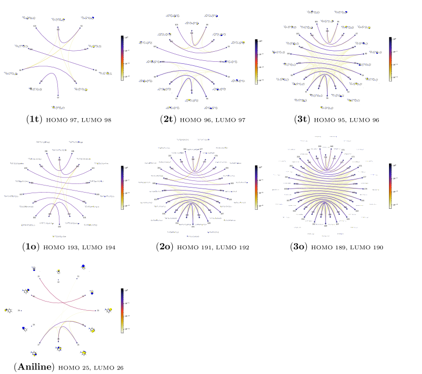
Figure 5: The orbital-pair mutual information for aniline and all investigated PANIs in their tetramer (t) and octamer (o) forms calculated from the pCCD ground-state wavefunctions within the PyBEST software package.

IV Conclusions

In this article, we employed modern quantum chemistry methods to investigate the electronic structures and properties, such as vibrational and electronic spectra, of the aniline molecule and PANIs at different oxidation states and lengths. We analyzed their structure-to-property relationship for the first time.

The BP86-optimized electronic structures and vibrational frequencies of aniline and PANIs are in excellent agreement with the available experimental data. The characteristic structural and vibrational features of PANIs in the tetramer form (1t, 2t, and 3t) are almost indistinguishable from their octamer counterparts (1o, 2o and 3o). Thus, the tetramer forms of PANIs are adequate models for longer polymer chains when considering structural and vibrational features, regardless of their oxidation states. However, the length of the PANI chain profoundly affects the electronic spectra and the overall electronic structure. Moving from aniline to polymeric structures, we observe an increased multi-reference character of the systems, which calls into question the reliability of DFAs in predicting excitation energies. Indeed, the CAM-B3LYP results for the octamer forms of PANI (1o, 2o, and 3o) failed to converge already for the ground state electronic structures. As an alternative, we propose to use pCCD-based methods that utilize the complete set of variationally optimized orbitals at the correlated level and can cope with such complex electronic structures. An additional advantage of pCCD-based methods is optimizing all orbitals (up to a thousand basis functions in this work). The final orbitals are localized, allowing us to dissect the character of the electronic transitions of each PANIs structure for the first time. Our results highlight the strong structure-to-property relationship for electronic excitations, where the character of the excited states changes upon polymer elongation of the oxidized forms of PANIs. For instance, elongating the polymer 2 delocalizes the leading transitions of the first excited state over the whole quinoid ring (2o), while 2t features leading transitions to the quinoid $\pi_{\rm N}^{*}$ orbital. Similarly, the first excited state in 3 changes its character upon polymer elongation. While 3t features more delocalized leading transitions from the N LPs to the benzenoid rings, the dominant transitions in 3o are centered on the quinoid ring.

V Conflicts of interest

There are no conflicts to declare.

VI Acknowledgment

S.J. and P.T. acknowledge financial support from the SONATA BIS research grant from the National Science Centre, Poland (Grant No. 2021/42/E/ST4/00302). P.T. acknowledges the scholarship for outstanding young scientists from the Ministry of Science and Higher Education. The research leading to these results has received funding from the Norway Grants 2014–2021 via the National Centre for Research and Development.

The authors thank Julia Romanova for providing us with the initial xyz structures of polyanilines. Calculations have been carried out using resources provided by the Wroclaw Centre for Networking and Supercomputing (http://wcss.pl), grant no. 411.

References

- Salikhov et al. (2018) R. B. Salikhov, Y. N. Biglova and A. G. Mustafin, InTech, 2018, 83–104.
- Chiang et al. (1977) C. K. Chiang, C. R. Fincher, Y. W. Park, A. J. Heeger, H. Shirakawa, E. J. Louis, S. C. Gau and A. G. MacDiarmid, Phys. Rev. Lett., 1977, 39, 1098–1101.
- Shirakawa (2001) H. Shirakawa, Rev. Mod. Phys., 2001, 73, 713–718.
- Kulkarni et al. (1989) V. G. Kulkarni, L. D. Campbell and W. R. Mathew, Synth. Met., 1989, 30, 321–325.
- Kulkarni et al. (1991) V. G. Kulkarni, W. R. Mathew, B. Wessling, H. Merkle and S. Blaettner, Synth. Met., 1991, 41, 1009–1012.
- Li et al. (2009) D. Li, J. Huang and R. B. Kaner, Acc. Chem. Res., 2009, 42, 135–145.
- Mishra (2015) A. K. Mishra, J. Comput. Sci., 2015, 10, 195–208.
- Ray et al. (1989) A. Ray, G. Asturias, D. Kershner, A. Richter, A. MacDiarmid and A. Epstein, Synth. Met., 1989, 29, 141–150.
- Chen et al. (2012) S. Chen, Z. Wei, X. Qi, L. Dong, Y.-G. Guo, L. Wan, Z. Shao and L. Li, J. Am. Chem. Soc., 2012, 134, 13252–13255.
- Wu et al. (2012) G. Wu, N. H. Mack, W. Gao, S. Ma, R. Zhong, J. Han, J. K. Baldwin and P. Zelenay, J. Am. Chem. Soc. Nano., 2012, 6, 9764–9776.
- Silakhori et al. (2013) M. Silakhori, M. S. Naghavi, H. S. C. Metselaar, T. M. I. Mahlia, H. Fauzi and M. Mehrali, Mater., 2013, 6, 1608–1620.
- Liu et al. (2013) M. Liu, Y.-E. Miao, C. Zhang, W. W. Tjiu, Z. Yang, H. Peng and T. Liu, Nanoscale, 2013, 5, 7312–7320.
- Ates (2013) M. Ates, Mater. Sci. Eng. C., 2013, 33, 1853–1859.
- Ameen et al. (2010) S. Ameen, M. S. Akhtar, Y. S. Kim, O.-B. Yang and H.-S. Shin, J. Phys. Chem. C., 2010, 114, 4760–4764.
- Zou et al. (2009) Y. Zou, J. Pisciotta, R. B. Billmyre and I. V. Baskakov, Biotechnol. Bioeng., 2009, 104, 939–946.
- Khalil (2001) H. S. A. Khalil, Ph.D. thesis, Polytechnic University, 2001.
- Quillard et al. (1994) S. Quillard, G. Louarn, S. Lefrant and A. MacDiarmid, Phys. Rev. B., 1994, 50, 12496.
- A. G. Macdiarmid (1987) A. F. R. A. G. Macdiarmid, J. C. Chiang, Synth. Met., 1987, 18, 285–290.
- Lim et al. (2000) S. Lim, K. Tan, E. Kang and W. Chin, J. Chem. Phys., 2000, 112, 10648–10658.
- Cihan Sorkun et al. (2022) M. Cihan Sorkun, D. Mullaj, J. V. A. Koelman and S. Er, Chemistry–Methods, 2022, e202200005.
- Genies et al. (1990) E. Genies, A. Boyle, M. Lapkowski and C. Tsintavis, Synth. Met., 1990, 36, 139–182.
- Bhadra and Khastgir (2008) S. Bhadra and D. Khastgir, Polym. Test., 2008, 27, 851–857.
- Shacklette et al. (1988) L. Shacklette, J. Wolf, S. Gould and R. Baughman, J. Chem. Phys., 1988, 88, 3955–3961.
- Moon and Park (1998) H.-S. Moon and J.-K. Park, J. Polym. Sci. A Polym. Chem., 1998, 36, 1431–1439.
- Sjögren and Stafström (1988) B. Sjögren and S. Stafström, J. Chem. Phys., 1988, 88, 3840–3847.
- de Oliveira Jr and Dos Santos (2000) Z. T. de Oliveira Jr and M. Dos Santos, Chem. Phys., 2000, 260, 95–103.
- Zhekova et al. (2007) H. Zhekova, A. Tadjer, A. Ivanova, J. Petrova and N. Gospodinova, Int. J. Quantum Chem., 2007, 107, 1688–1706.
- Jansen et al. (1999) S. A. Jansen, T. Duong, A. Major, Y. Wei and L. T. Sein Jr, Synth. Met., 1999, 105, 107–113.
- Foreman and Monkman (2003) J. P. Foreman and A. P. Monkman, J. Phys. Chem. A, 2003, 107, 7604–7610.
- Mishra and Tandon (2009) A. K. Mishra and P. Tandon, J. Phys. Chem. B, 2009, 113, 14629–14639.
- Romanova et al. (2010) J. Romanova, J. Petrova, A. Ivanova, A. Tadjer and N. Gospodinova, J. Mol. Struct., 2010, 954, 36–44.
- Zhang et al. (2017) Y. Zhang, Y. Duan and J. Liu, Spectrochim. Acta A Mol. Biomol. Spectrosc., 2017, 171, 305–310.
- Limacher et al. (2013) P. A. Limacher, P. W. Ayers, P. A. Johnson, S. De Baerdemacker, D. Van Neck and P. Bultinck, J. Chem. Theory Comput., 2013, 9, 1394–1401.
- Stein et al. (2014) T. Stein, T. M. Henderson and G. E. Scuseria, J. Chem. Phys., 2014, 140, 214113.
- Tecmer and Boguslawski (2022) P. Tecmer and K. Boguslawski, Phys. Chem. Chem. Phys., 2022, 24, 23026–23048.
- Tecmer and Boguslawski (2022) P. Tecmer and K. Boguslawski, Phys. Chem. Chem. Phys., 2022, 24, 23026–23048.
- K. Boguslawski, P. Tecmer (2017) K. Boguslawski, P. Tecmer, Int. J. Quantum Chem., 2017, 117, e25455.
- Boguslawski and Tecmer (2015) K. Boguslawski and P. Tecmer, Int. J. Quantum Chem., 2015, 115, 1289–1295.
- Boguslawski et al. (2014) K. Boguslawski, P. Tecmer, P. W. Ayers, P. Bultinck, S. De Baerdemacker and D. Van Neck, Phys. Rev. B, 2014, 89, 201106(R).
- Boguslawski et al. (2014) K. Boguslawski, P. Tecmer, P. A. Limacher, P. A. Johnson, P. W. Ayers, P. Bultinck, S. De Baerdemacker and D. Van Neck, J. Chem. Phys., 2014, 140, 214114.
- Boguslawski et al. (2014) K. Boguslawski, P. Tecmer, P. Bultinck, S. De Baerdemacker, D. Van Neck and P. W. Ayers, J. Chem. Theory Comput., 2014, 10, 4873–4882.
- Tecmer et al. (2014) P. Tecmer, K. Boguslawski, P. A. Limacher, P. A. Johnson, M. Chan, T. Verstraelen and P. W. Ayers, J. Phys. Chem. A, 2014, 118, 9058–9068.
- Tecmer et al. (2015) P. Tecmer, K. Boguslawski and P. W. Ayers, Phys. Chem. Chem. Phys., 2015, 17, 14427–14436.
- Tecmer et al. (2019) P. Tecmer, K. Boguslawski, M. Borkowski, P. S. Żuchowski and D. Kȩdziera, Int. J. Quantum Chem., 2019, 119, e25983.
- Rowe (1968) D. J. Rowe, Rev. Mod. Phys., 1968, 40, 153–166.
- Stanton and Bartlett (1993) J. F. Stanton and R. J. Bartlett, J. Chem. Phys., 1993, 98, 7029–7039.
- Boguslawski (2016) K. Boguslawski, J. Chem. Phys., 2016, 145, 234105.
- Boguslawski (2017) K. Boguslawski, J. Chem. Phys., 2017, 147, 139901.
- Boguslawski (2019) K. Boguslawski, J. Chem. Theory Comput., 2019, 15, 18–24.
- Watts and Bartlett (1994) J. D. Watts and R. J. Bartlett, J. Chem. Phys., 1994, 101, 3073–3078.
- Ahlrichs et al. (1989) R. Ahlrichs, M. Bär, M. Häser, H. Horn and C. Kölmel, Chem. Phys. Lett., 1989, 162, 165.
-
(52)
TURBOMOLE V6.6, a development of University of Karlsruhe and
Forschungszentrum Karlsruhe GmbH, 1989-2022, TURBOMOLE GmbH, since 2007;
available from
http://www.turbomole.com. - Perdew (1986) J. Perdew, Phys. Rev. B, 1986, 33, 8822–8824.
- Becke (1988) A. Becke, Phys. Rev. A, 1988, 38, 3098–4000.
- F. Weigend, R. Ahlrichs (2005) F. Weigend, R. Ahlrichs, Phys. Chem. Chem. Phys., 2005, 7, 3297–3305.
- Weigend (1998) F. Weigend, Chem. Phys. Lett., 1998, 294, 143–152.
- Runge and Gross (1984) E. Runge and E. K. U. Gross, Phys. Rev. Lett., 1984, 52, 997–100.
- Van Gisbergen et al. (1999) S. Van Gisbergen, J. Snijders and E. Baerends, Comput. Phys. Commun., 1999, 118, 119–138.
- te Velde et al. (2001) G. te Velde, F. M. Bickelhaupt, E. J. Baerends, C. F. Guerra, S. J. A. van Gisbergen, J. G. Snijders and T. Ziegler, J. Comput. Chem., 2001, 22, 931–967.
- adf (2018) 2018, ADF2018.01, SCM, Theoretical Chemistry, Vrije Universiteit, Amsterdam, The Netherlands, http://www.scm.com.
- Perdew et al. (1996) J. P. Perdew, K. Burke and M. Ernzerhof, Phys. Rev. Lett., 1996, 77, 3865.
- Adamo and Barone (1999) C. Adamo and V. Barone, J. Chem. Phys., 1999, 110, 6158–6170.
- Yanai et al. (2004) T. Yanai, D. P. Tew and N. C. Handy, Chem. Phys. Lett., 2004, 393, 51–57.
- van Lenthe and Baerends (2003) E. van Lenthe and E. J. Baerends, J. Comput. Chem., 2003, 24, 1142–1156.
- Boguslawski et al. (2021) K. Boguslawski, A. Leszczyk, A. Nowak, F. Brzȩk, P. S. Żuchowski, D. Kȩdziera and P. Tecmer, Comput. Phys. Commun., 2021, 264, 107933.
- (66) K. Boguslawski, A. Leszczyk, A. Nowak, E. Sujkowski, F. Brzȩk, P. S. Źuchowski, D. Kȩdziera and P. Tecmer, PyBESTv.1.2.0.
- Dunning Jr. (1989) T. Dunning Jr., J. Chem. Phys., 1989, 90, 1007–1023.
- Pipek and Mezey (1989) J. Pipek and P. G. Mezey, J. Chem. Phys., 1989, 90, 4916–4926.
- Bytautas et al. (2003) L. Bytautas, J. Ivanic and K. Ruedenberg, J. Chem. Phys., 2003, 119, 8217–8224.
- K. Boguslawski, P. Tecmer (2015) K. Boguslawski, P. Tecmer, Int. J. Quantum Chem., 2015, 115, 1289–1295.
- Boguslawski et al. (2013) K. Boguslawski, P. Tecmer, G. Barcza, O. Legeza and M. Reiher, J. Chem. Theory Comput., 2013, 9, 2959–2973.
- Nowak et al. (2021) A. Nowak, O. Legeza and K. Boguslawski, J. Chem. Phys., 2021, 154, 084111.
- Rissler et al. (2006) J. Rissler, R. M. Noack and S. R. White, Chem. Phys., 2006, 323, 519–531.
- Szalay et al. (2015) S. Szalay, M. Pfeffer, V. Murg, G. Barcza, F. Verstraete, R. Schneider and Ö. Legeza, Int. J. Quantum Chem., 2015, 115, 1342–1391.
- Barcza et al. (2011) G. Barcza, O. Legeza, K. H. Marti and M. Reiher, Phys. Rev. A, 2011, 83, 012508.
- Ding et al. (2020) L. Ding, S. Mardazad, S. Das, S. Szalay, U. Schollwöck, Z. Zimborás and C. Schilling, J. Chem. Theory Comput., 2020, 17, 79–95.
- Boguslawski et al. (2016) K. Boguslawski, P. Tecmer and Ö. Legeza, Phys. Rev. B, 2016, 94, 155126.
- Nowak and Boguslawski (2023) A. Nowak and K. Boguslawski, Phys. Chem. Chem. Phys., 2023, 25, 7289–7301.
- Piest et al. (1999) H. Piest, G. von Helden and G. Meijer, J. Chem. Phys., 1999, 110, 2010–2015.
- Wojciechowski et al. (2003) P. M. Wojciechowski, W. Zierkiewicz, D. Michalska and P. Hobza, J. Chem. Phys., 2003, 118, 10900–10911.
- Cui et al. (2020) Y. Cui, P. Zhu, X. Liao and Y. Chen, J. Mat. Chem. C, 2020, 8, 15920–15939.
- Dreuw and Head-Gordon (2005) A. Dreuw and M. Head-Gordon, Chem. Rev., 2005, 105, 4009–4037.
- Laurent and Jacquemin (2013) A. D. Laurent and D. Jacquemin, Int. J. Quantum Chem., 2013, 113, 2019–2039.
- Körzdörfer and Brédas (2014) T. Körzdörfer and J.-L. Brédas, Acc. Chem. Res., 2014, 47, 3284–3291.
- Dreuw et al. (2003) M. Dreuw, J. L. Weisman and M. Head-Gordon, J. Chem. Phys., 2003, 119, 2943.
- Dreuw and Head-Gordon (2004) M. Dreuw and M. Head-Gordon, J. Am. Chem. Soc., 2004, 126, 4007–4016.
- Tecmer et al. (2011) P. Tecmer, A. S. P. Gomes, U. Ekström and L. Visscher, Phys. Chem. Chem. Phys., 2011, 13, 6249–6259.
- Tecmer et al. (2012) P. Tecmer, R. Bast, K. Ruud and L. Visscher, J. Phys. Chem. A, 2012, 116, 7397–7404.
- Tecmer et al. (2013) P. Tecmer, N. Govind, K. Kowalski, W. A. de Jong and L. Visscher, J. Chem. Phys, 2013, 139, 034301.
- Ben Amor et al. (2021) N. Ben Amor, S. Evangelisti, T. Leininger and D. Andrae, in Basis Sets in Computational Chemistry, Springer, 2021, pp. 41–101.
- Stewart (2019) J. J. Stewart, J. Mol. Model., 2019, 25, 7.