Augmented balancing weights as linear regression

Abstract

We provide a novel characterization of augmented balancing weights, also known as automatic debiased machine learning (AutoDML). These popular doubly robust or double machine learning estimators combine outcome modeling with balancing weights — weights that achieve covariate balance directly in lieu of estimating and inverting the propensity score. When the outcome and weighting models are both linear in some (possibly infinite) basis, we show that the augmented estimator is equivalent to a single linear model with coefficients that combine the coefficients from the original outcome model coefficients and coefficients from an unpenalized ordinary least squares (OLS) fit on the same data; in many real-world applications the augmented estimator collapses to the OLS estimate alone. We then extend these results to specific choices of outcome and weighting models. We first show that the augmented estimator that uses (kernel) ridge regression for both outcome and weighting models is equivalent to a single, undersmoothed (kernel) ridge regression. This holds numerically in finite samples and lays the groundwork for a novel analysis of undersmoothing and asymptotic rates of convergence. When the weighting model is instead lasso-penalized regression, we give closed-form expressions for special cases and demonstrate a “double selection” property. Our framework opens the black box on this increasingly popular class of estimators, bridges the gap between existing results on the semiparametric efficiency of undersmoothed and doubly robust estimators, and provides new insights into the performance of augmented balancing weights.

1 Introduction

Combining outcome modeling and weighting, as in augmented inverse propensity score weighting (AIPW) and other doubly robust (DR) or double machine learning (DML) estimators, is a core strategy for estimating causal effects using observational data. A growing body of literature finds weights by solving a “balancing weights” optimization problem to estimate weights directly, rather than by first estimating the propensity score and then inverting. The DR versions of these estimators are referred to by a number of terms, including augmented balancing weights (Athey et al., 2018; Hirshberg and Wager, 2021), automatic debiased machine learning (AutoDML; Chernozhukov et al., 2022d), and generalized regression estimators (GREG; Deville and Särndal, 1992); see Ben-Michael et al. (2021b) for a review. This strategy applies to a wide range of linear estimands via the Riesz representation theorem (e.g., Hirshberg and Wager, 2021; Chernozhukov et al., 2022e).

In this paper, we consider augmented balancing weights in which the estimators for both the outcome model and the balancing weights are based on penalized linear regressions in some possibly infinite basis; in addition to all high-dimensional linear models, this broad class includes popular nonparametric models such as kernel regression and certain forms of random forests and neural networks. We generalize existing results by proving that any linear balancing weights estimator is numerically equivalent to applying unregularized ordinary least squares (OLS) coefficient estimates to a re-weighted — rather than observed — target covariate profile.

We use this characterization to show that, somewhat surprisingly, augmenting any regularized linear outcome regression (the “base learner”) with linear balancing weights is numerically equivalent to a single linear outcome regression applied to the target covariate profile. The resulting coefficients are an affine (and often convex) combination of the base learner model coefficients and unregularized OLS coefficients; the hyperparameter for the balancing weights estimator directly controls the regularization path defining the affine combination. We specialize these results to ridge and lasso regularization and show that augmenting an outcome model with balancing weights often corresponds to a form of undersmoothing. We then show that our numerical results on undersmoothing for (kernel) ridge-augmented balancing weights offer a new perspective on the optimal asymptotic regularization schedule for undersmoothed ridge regression. Finally, we demonstrate the implications of these results on several causal inference benchmark data sets. For the canonical LaLonde (1986) study, we show that applying several off-the-shelf augmented balancing weights and AutoDML estimators can be numerically equivalent to estimating the effect with unregularized OLS alone, even if the outcome regression base learner is heavily regularized.

Our results provide important insights into the nexus of causal inference and machine learning. First, these results open the black box on the growing number of methods based on augmented balancing weights and AutoDML — methods that can sometimes be difficult to taxonomize or understand. We show that, under linearity, these estimators all share an underlying and very simple structure. Our results highlight that estimation choices for augmented balancing weights can lead to potentially unexpected behavior. Most notably, the choice of (kernel) ridge regression for both outcome and weighting models collapses to a single (kernel) ridge regression estimator. This is a generalization of the argument in Robins et al. (2007) that “OLS is doubly robust” to a much broader class of penalized parametric and non-parametric regression models. At a high level, as causal inference moves towards incorporating machine learning and automation, our work highlights how the traditional lines between weighting and regression-based approaches are becoming increasingly blurred.

Second, our results connect two approaches to “automate” semiparametric causal inference. AutoDML and related methods exploit the fact that we can estimate a Riesz representer without a closed form expression for a wide class of functionals. The estimated Riesz representer then augments a base learner by bias correcting a plug-in estimator of the functional. Older approaches, such as undersmoothing (Goldstein and Messer, 1992; Newey et al., 1998), twicing kernels (Newey et al., 2004), and sieve estimation (Newey, 1994; Shen, 1997), also avoid estimation of the Riesz representer, tuning the base learner regression fit such that an additional bias correction is not required. Achieving this optimal tuning in practice has long been a hurdle for the implementation of these methods. Subject to certain conditions, both approaches can yield estimators that are asymptotically efficient. We show that if all required tuning parameters are defined in terms of an $\ell_{2}$-norm constraint, then these two approaches can be numerically identical even in finite samples. This is a surprising result that may have implications for optimal undersmoothing tuning parameter selection.

In Section 2 we introduce the problem setup, identification assumptions, and common estimation methods; we also review balancing weights and previous results linking balancing weights to outcome regression models. In Section 3 we present our new results, and in Sections 4 and 5 we cache out the implications for $\ell_{2}$ and $\ell_{\infty}$ balancing weights specifically. Section 6 gives a numeric illustration. Section 7 gives some implications of our results for the asymptotics of kernel ridge regression. Section 8 discusses the connection with the semiparametrics literature and offers some other directions for future research. The appendix includes extensive additional technical discussion and extensions.

1.1 Related work

Balancing weights and AutoDML.

With deep roots in survey calibration methods and the generalized regression estimator (GREG; see Deville and Särndal, 1992; Lumley et al., 2011; Gao et al., 2022), a large and growing causal inference literature uses balancing weights estimation in place of traditional inverse propensity score weighting (IPW). Ben-Michael et al. (2021b) provide a recent review; we discuss specific examples at length in Section 2.3 below. This approach typically tries to achieve minimax finite-sample balance of features of the covariate distributions in the different treatment groups. Of particular interest here are augmented balancing weights estimators that combine balancing weights with outcome regression; see, for example, Athey et al. (2018); Hirshberg and Wager (2021); Ben-Michael et al. (2021c).

A parallel literature in econometrics instead focuses on so-called automatic estimation of the Riesz representer, of which IPW are a special case, where “automatic” refers to the fact that we can estimate the Riesz representer without obtaining a closed form expression. The corresponding augmented estimation framework is known as Automatic Debiased Machine Learning, or AutoDML; see, among others, Chernozhukov et al. (2022a), Chernozhukov et al. (2022b), Chernozhukov et al. (2022d), and Chernozhukov et al. (2022e). This approach has also been applied in a range of settings, including to corrupted data (Agarwal and Singh, 2021), to dynamic treatment regimes (Chernozhukov et al., 2022c), and to address noncompliance (Singh et al., 2022). As we discuss in Appendix C.3, the AutoDML approach nearly always employs cross-fitting and is typically motivated by asymptotic properties rather than achieving balance in finite samples.

Numerical equivalences for balancing weights.

Many seminal papers highlight connections between weighting approaches, such as balancing weights and IPW, and outcome modeling; see Bruns-Smith and Feller (2022) for discussion. Most relevant are a series of papers that show numerical equivalences between linear regression and (exact) balancing weights, especially Robins et al. (2007); Kline (2011); Chattopadhyay and Zubizarreta (2021), and between kernel ridge regression and forms of kernel weighting (Kallus, 2020; Hirshberg et al., 2019). We discuss these equivalences at length in Appendix A. Finally, as we discuss in Appendix D, there are close connections between balancing weights and Empirical Likelihood (Hellerstein and Imbens, 1999; Newey and Smith, 2004).

2 Problem setup and background

2.1 Setup and motivation

Our paper proves new numeric equivalences for existing estimation procedures, and as such the results hold absent any causal assumptions or statistical model. However, a primary motivation for this work is the task of estimating unobserved counterfactual means in causal inference. We briefly review this setting here and use it as a running example throughout, emphasizing that this is purely for interpretation. We begin with the canonical case of estimating a counterfactual mean under conditional ignorability, and then turn to the more general setup of estimating linear functionals via the Riesz representer.

2.1.1 Warmup: counterfactual means

Let $X,Y,Z$ be random variables defined on $\mathcal{X},\mathbb{R},\mathcal{Z}$ with joint probability distribution $p$. To begin, consider the example of a binary treatment, $\mathcal{Z}=\{0,1\}$ and covariates $X$. Define potential or counterfactual outcomes $Y(1)$ and $Y(0)$ under assignment to treatment and control, respectively. Under SUTVA (Rubin, 1980), we observe outcomes $Y=ZY(1)+(1-Z)Y(0)$. To estimate the average treatment effect, $\mathbb{E}[Y(1)-Y(0)]$, we first estimate the means of the partially observed potential outcomes, $\mathbb{E}[Y(1)]$ and $\mathbb{E}[Y(0)]$.

Let $m(x,z)\coloneqq\mathbb{E}[Y\mid X=x,Z=z]$ be the outcome model, $e_{z}(x)\coloneqq\mathbb{P}[Z=1\mid X=x]$ be the propensity score, and $\alpha(x,z)=z/e(x)$ be the inverse propensity score weights (IPW). Under the additional assumptions of conditional ignorability, $Y(1)\mathchoice{\mathrel{\hbox to0.0pt{$\displaystyle\perp$\hss}\mkern 2.0mu{\displaystyle\perp}}}{\mathrel{\hbox to0.0pt{$\textstyle\perp$\hss}\mkern 2.0mu{\textstyle\perp}}}{\mathrel{\hbox to0.0pt{$\scriptstyle\perp$\hss}\mkern 2.0mu{\scriptstyle\perp}}}{\mathrel{\hbox to0.0pt{$\scriptscriptstyle\perp$\hss}\mkern 2.0mu{\scriptscriptstyle\perp}}}Z\mid X$, and overlap, $\mathbb{E}[\alpha(X,Z)^{2}]<\infty$, we have that $\mathbb{E}[Y(1)]$ is identified by $\mathbb{E}[m(X,1)]$, a (linear) functional of the observed data distribution. A symmetric argument holds for $\mathbb{E}[Y(0)]$.

There are three broad strategies for estimating $\mathbb{E}[Y(1)]$. First, the identifying functional above suggests estimating the outcome model, $m(x,1)$ among those units with $Z=1$, and plugging this into the regression functional, $\mathbb{E}[m(X,1)]$. Second, the equality $\mathbb{E}[m(X,1)]=\mathbb{E}[Z/e(X)Y]=\mathbb{E}[\alpha(X,Z)Y]$ suggests estimating the inverse propensity score weights, $\alpha(x,z)=z/e(x)$, and plugging these into the weighting functional. Finally, we can combine these two via the doubly robust functional (Robins et al., 1994):

$$\mathbb{E}[m(X,1)+\alpha(X,Z)(Y-m(X,1)].$$

This functional has the attractive property of being equal to $\mathbb{E}[m(X,1)]$ even if either one of $\alpha$ or $m$ is replaced with an arbitrary function of $X$ and $Z$, hence the term “doubly robust.” See Chernozhukov et al. (2018); Kennedy (2022) for recent overviews of the active literature in causal inference and machine learning focused on estimating versions of this functional.

2.1.2 General linear functionals via the Riesz representer

The setup above used causal assumptions to identify the mean potential outcome $\mathbb{E}[Y(1)]$ as a linear functional of the observed data distribution $\mathbb{E}[m(X,1)]$. A recent literature (e.g., Hirshberg and Wager, 2021; Chernozhukov et al., 2022d) emphasizes that we can generalize this approach to estimate a wide range of linear functionals of the data. In particular, we now let $\mathcal{Z}$ be an arbitrary set and let $Z$ be a random variable with support $\mathcal{Z}$. Our goal is to estimate a linear functional of the form:

$$\psi(m)=\mathbb{E}[h(X_{i},Z_{i},m)],$$ (1)

where $h$ is a real-valued, mean-squared continuous linear functional of $m$.

Following Chernozhukov et al. (2022d, e), we can generalize the weighting functional to this general class of estimands via the Riesz representer, which is a function $\alpha(X,Z)\in L_{2}(p)$ such that, for all square-integrable functions $f\in L_{2}(p)$:

$$\mathbb{E}[h(X,Z,f)]=\mathbb{E}[\alpha(X,Z)f(X,Z)].$$ (2)

To make this more concrete, consider the following three examples.

Example 1 (Counterfactual mean).

Let $Z=\{0,1\}$ and $\psi(m)=\mathbb{E}[m(X,1)].$ Under SUTVA and conditional ignorability, this estimand is equal to $E[Y(1)]$. The Riesz representer is the IPW, $\alpha(X,Z)=Z/e(X)$.

Example 2 (Average derivative).

Let $Z\in\mathbb{R}$ and $\psi(m)=\mathbb{E}\left[\frac{\partial}{\partial z}m(X,Z)\right].$ Under an appropriate generalization of SUTVA and conditional ignorability, this estimand corresponds to the average derivative effect of a continuous treatment. Under regularity conditions the Riesz representer is given by $\alpha(X,Z)=-\frac{\frac{d}{dz}p(Z|X)}{p(Z|X)}$ where $p(z|x)$ is the conditional density of $Z$ given $X$.

Example 3 (Distribution shift).

Consider an example without $Z$, following the machine learning literature on covariate shift. Let $p$ denote the source distribution of the observed data, and let $p^{\ast}$ over $\mathcal{X}$ denote the target distribution. The estimand is then $\psi(m)=\int_{\mathcal{X}}m(x)dp^{\ast}(x)$. In a causal inference setting, this can recover the Average Treatment Effect on the Treated (ATT) under SUTVA and conditional ignorability; i.e., let $p$ be the distribution of covariates and outcomes for units assigned to control and $p^{\ast}$ be the distribution of the covariates for units assigned to treatment. The Riesz representer is the density ratio, $\alpha(X)=\frac{dp^{\ast}}{dp}(X)$.

As in the counterfactual mean example, we can identify this more general target functional via the outcome model functional in (1), via the Riesz representer functional in (2) with $f=m$, or via the doubly robust functional

$$\mathbb{E}[h(X,Z,m)+\alpha(X,Z)(Y-m(X,Z))].$$ (3)

Estimators of this DR functional are augmented in the sense that they augment the “plug-in,” “outcome regression,” or “base learner” estimator $\mathbb{E}[h(X,Z,m)]$ with appropriately weighted residuals; or, equivalently, that augment the weighting estimator with an appropriate outcome regression. This is the class of estimators to which our results apply.

2.2 Balancing weights: Background and general form

The balancing weights framework, also known as automatic estimation of the Riesz representer, estimates the Riesz representer directly — rather than estimating it via an analytic functional form, e.g., by estimating the propensity score and inverting it (Ben-Michael et al., 2021b; Chernozhukov et al., 2022d). This approach does not require a known analytic form (Chernozhukov et al., 2022e), is often much more stable (Zubizarreta, 2015), and offers improved control of finite sample covariate imbalance (Zhao, 2019).

Weighting for balance.

A central property of the Riesz representer is that the corresponding weights, $w(X,Z)=\alpha(X,Z)$, are the unique weights that satisfy the population balance property property in Equation 2 for all square-integrable functions $f\in L_{2}(p)$. To see why this rather abstract equality is known as a balance property, consider the case of a missing mean in Example 3: weighting the source population observations with the Riesz representer balances the covariate distributions in the source and target populations by making the source population distribution perfectly match the target population distribution.

We can use this property to characterize $\alpha(X,Z)$ as the unique solution to the optimization problem:

$$\underset{w\in L_{2}(p)}{\text{min}}~{}\underset{f\in L_{2}(p)}{\text{sup}}\Big{\{}\mathbb{E}[w(X,Z)f(X,Z)]-\mathbb{E}[h(X,Z,f)]\Big{\}},$$ (4)

where the objective is called the “imbalance.” However, this does not lead to a practical estimator: due to the flexibility of $L_{2}(p)$, the inner supremum can behave erratically for $w\neq\alpha(X,Z)$.

We make this problem more tractable by imposing simplifying assumptions on the nature of confounding. In particular, for our target estimand $\psi(m)$ we only need to satisfy the condition in Equation 2 for the special case of $f=m$. If we are willing to assume that $m$ lies in a model class $\mathcal{F}\subset L_{2}(p)$, then it suffices to balance functions in that class, and we can replace the objective in (4) with the imbalance over $\mathcal{F}$:

$$\text{Imbalance}_{\mathcal{F}}(w)\coloneqq\sup_{f\in\mathcal{F}}\Big{\{}\mathbb{E}[w(X,Z)f(X,Z)]-\mathbb{E}[h(X,Z,f)]\Big{\}}.$$ (5)

Typically, the balancing weights approach also introduces a regularization hyperparameter $\delta>0$ to ensure a unique minimum and to introduce a bias-variance trade-off. The resulting balancing weights are the unique solution $w^{*}$ to the following strictly-convex optimization problem (see Appendix D for alternative variants):

$$\min_{w\in L_{2}(p)}\Big{\{}\text{Imbalance}_{\mathcal{F}}(w)+\delta\|w\|^{2}\Big{\}}.$$ (6)

If the true conditional expectation $m\in\mathcal{F}$, then the imbalance $\Big{\{}\mathbb{E}[w^{*}(X,Z)m(X,Z)]-\mathbb{E}[h(X,Z,m)]\Big{\}}$, will be small and thus $\mathbb{E}[w^{*}(X,Z)Y]$ is an approximately unbiased estimate of $\mathbb{E}[h(X,Z,m)]$. For a more formal statement, see, for example, Hirshberg and Wager (2021).

Direct estimation of the Riesz representer.

Chernozhukov et al. (2022d) consider an alternative motivation for balancing weights: estimating the Riesz representer directly by finding weights $f$ that directly minimize the mean-squared error for $\alpha(X,Z)$,

$$\min_{f\in\mathcal{F}}\left\{\mathbb{E}\left[\left(f(X,Z)-\alpha(X,Z)\right)^{2}\right]\right\}.$$ (7)

With the introduction of a hyperparameter (see (8) below), this problem is equivalent to the optimization problem in Equation (6).

2.3 Linear balancing weights

2.3.1 Population balance

In this paper, we consider the special case where the outcome models are linear in some basis expansion of $X$ and $Z$. This is an extremely broad class that encompasses linear and polynomial models of arbitrary functions of $X$ and $Z$ and with dimension possibly larger than the sample size, as well as non-parametric models such as reproducing kernel Hilbert spaces (RKHSs; Gretton et al., 2012), the Highly-Adaptive Lasso (Benkeser and Van Der Laan, 2016), the neural tangent kernel space of infinite-width neural networks (Jacot et al., 2018), and “honest” random forests (Agarwal et al., 2022). However, this class excludes models for $m$ that are fundamentally non-linear in their parameters, like general neural networks or generalized linear models passed through a non-linear link function. We extend our results to arbitrary nonlinear balancing weights in Appendix D.

Define the feature map $\phi:\mathcal{X}\times\mathcal{Z}\rightarrow\mathbb{R}^{d}$ and let $\phi_{j}:\mathcal{X}\times\mathcal{Z}\rightarrow\mathbb{R}$ denote the mapping for the $j$th feature. Let $\mathcal{F}=\{f(x,z)=\theta^{\top}\phi(x,z):\|\theta\|\leq 1\}$ where $\|\cdot\|$ can be any norm on $\mathbb{R}^{d}$. The general setup constrains $\|\theta\|\leq r$; we set $r=1$ without loss of generality, which simplifies exposition below. Let $\|\cdot\|_{*}$ be the dual norm of $\|\cdot\|$; that is, $\|v\|_{*}\coloneqq\sup_{\|u\|\leq 1}u^{\top}v.$ Many common vector norms have familiar, closed-form, dual norms, e.g., the dual norm of the $\ell_{2}$-norm is the $\ell_{2}$-norm; and the dual norm of the $\ell_{1}$-norm is the $\ell_{\infty}$-norm.

Under linearity, the imbalance over all $f\in\mathcal{F}$ has a simple closed form. For any $f(x,z)=\theta^{\top}\phi(x,z)\in\mathcal{F}$, $\mathbb{E}[h(X,Z,f)]=\theta^{\top}\mathbb{E}[h(X,Z,\phi)],$ where $h(X,Z,\phi)$ is short-hand for the vector with $j$th entry $h(X,Z,\phi_{j})$. We can then write the imbalance in terms of the transformed feature space $h(X,Z,\phi)$; following the balancing weights literature, we refer to this quantity as the target features. Applying the linear functional $\psi$ from (1) to the features $\phi$, we have the following closed form:

$$\text{Imbalance}_{\mathcal{F}}(w) \coloneqq\sup_{f\in\mathcal{F}}\Big{\{}\mathbb{E}[w(X,Z)f(X,Z)]-\mathbb{E}[h(X,Z,f)]\Big{\}}$$

$$=\sup_{\|\theta\|\leq 1}\Big{\{}\theta^{\top}\mathbb{E}[w(X,Z)\phi(X,Z)]-\theta^{\top}\mathbb{E}[h(X,Z,\phi)]\Big{\}}$$

$$=\big{\|}\mathbb{E}[w(X,Z)\phi(X,Z)]-\mathbb{E}[h(X,Z,\phi)]\big{\|}_{*}.$$

For instance, for the missing counterfactual mean in Example 1, $h(X,Z,m)=m(X,1)$. The imbalance is then the difference between the re-weighted features from the whole population, $w(X,Z)\phi(X,Z)$, and the target features with $Z=1$, $\phi(X,1)$.

2.3.2 Finite sample balance

Because our results concern numeric equivalences, we will focus on the finite sample version of the linear balancing weights problem. Let $X_{p},Y_{p},Z_{p}$ be $n$ i.i.d. samples from the distribution $p$ of the observed data, and denote $\Phi_{p}\coloneqq\phi(X_{p},Z_{p})$. Let $\Phi_{q}\coloneqq h(X_{p},Z_{p},\phi)$ denote the target features. We will write $\hat{\mathbb{E}}$ for sample averages; define $\mkern 1.5mu\overline{\mkern-1.5mu\Phi\mkern-1.5mu}\mkern 1.5mu_{p}\coloneqq\hat{\mathbb{E}}[\Phi_{p}]$ and $\mkern 1.5mu\overline{\mkern-1.5mu\Phi\mkern-1.5mu}\mkern 1.5mu_{q}\coloneqq\hat{\mathbb{E}}[\Phi_{q}]$. For exposition, we assume that $d<n$ and that $\Phi_{p}$ has rank $d$. We emphasize that this is not necessary for our results — one can replace $\mathbb{R}^{d}$ with an infinite-dimensional Hilbert space $\mathcal{H}$ and relax the rank restriction. See Appendix B for a formal presentation of the high-dimensional setting.

In what follows we write $w$ for the $1\times n$ vector $w(\Phi_{p})$, to highlight the fact that we will estimate $w$ directly rather than as an explicit function of $X$ or $\Phi_{p}$. Using the derivation above, we can directly calculate the finite sample imbalance as:

$$\widehat{\text{Imbalance}_{\mathcal{F}}}(w)=\|\tfrac{1}{n}w\Phi_{p}-\bar{\Phi}_{q}\|_{*}.$$

Now we can write the balancing weights optimization problem in (6) equivalently as either:

Penalized form: $$\min_{w\in\mathbb{R}^{n}}\Big{\{}\|\tfrac{1}{n}w\Phi_{p}-\bar{\Phi}_{q}\|^{2}_{*}+\delta_{1}\|w\|_{2}^{2}\Big{\}}$$

Constrained form: $$\min_{w\in\mathbb{R}^{n}}\|w\|_{2}^{2}$$

$$\text{such that }\|\tfrac{1}{n}w\Phi_{p}-\bar{\Phi}_{q}\|_{*}\leq\delta_{2}.$$

Furthermore, we can write the equivalent problem in (7) as:

Automatic form: $$\min_{\theta\in\mathbb{R}^{d}}\Big{\{}\tfrac{1}{n}\theta^{\top}(\Phi_{p}^{\top}\Phi_{p})\theta-\tfrac{1}{n}2\theta^{\top}\bar{\Phi}_{q}+\delta_{3}\|\theta\|\Big{\}},$$ (8)

where we use the terminology “automatic” from Chernozhukov et al. (2022d). For any parameter $\delta_{2}>0$ and corresponding constrained problem solution $\hat{w}$, there exists a parameter $\delta_{3}>0$ such that $\hat{w}=\delta_{3}\Phi_{p}\hat{\theta}$, where $\hat{\theta}$ is the solution to the automatic form. As a result, for any norm $\|\cdot\|$, the penalized and constrained forms will always produce weights that are linear in $\Phi_{p}$ (Ben-Michael et al., 2021b). Without loss of generality, we therefore use $\delta$ to denote the regularization parameter for the balancing weights problem, regardless of the specific form. We now illustrate several common choices for this problem; in Appendix D we discuss popular forms of balancing that constrain the weights to be non-negative.

Example 4 (Exact balancing weights).

The most common balancing weights estimation problem finds the minimum weights that exactly balance each element of $\Phi$. In the constrained form, exact balancing solves

$$\min_{w\in\mathbb{R}^{n}}\|w\|_{2}^{2}$$ (9)

$$\text{such that }\tfrac{1}{n}w\phi_{pj}=\bar{\phi}_{qj}\quad\text{ for all }j$$

Example 5 ($\ell_{2}$ balancing).

The $\ell_{2}$ balancing weights problem is usually expressed via its penalized form:

$$\min_{w\in\mathbb{R}^{n}}\Big{\{}\|\tfrac{1}{n}w\Phi_{p}-\mkern 1.5mu\overline{\mkern-1.5mu\Phi\mkern-1.5mu}\mkern 1.5mu_{q}\|^{2}_{2}+\delta\|w\|_{2}^{2}\Big{\}}.$$ (10)

The automatic form is a ridge-penalized regression for the Riesz representer.

Example 6 ($\ell_{\infty}$ balancing).

The constrained form of the $\ell_{\infty}$ balancing weights problem is

$$\min_{w\in\mathbb{R}^{n}}\|w\|_{2}^{2}$$ (11)

$$\text{such that }\|\tfrac{1}{n}w\Phi_{p}-\mkern 1.5mu\overline{\mkern-1.5mu\Phi\mkern-1.5mu}\mkern 1.5mu_{q}\|_{\infty}\leq\delta$$

The automatic form is a lasso-penalized regression for the Riesz representer, sometimes known as the Minimum Distance Lasso (Chernozhukov et al., 2022d).

Example 7 (Kernel balancing).

As a brief preview of the balancing problem in the infinite-dimensional setting, we provide an example where $\mathcal{F}=\mathcal{H}$ is a reproducing kernel Hilbert space on $\mathcal{X}\times\mathcal{Z}$ with norm $\|\cdot\|_{\mathcal{H}}$ and kernel $\mathcal{K}:(\mathcal{X}\times\mathcal{Z})\times(\mathcal{X}\times\mathcal{Z})\rightarrow\mathbb{R}$. Then for any $x_{i}\in\mathcal{X},z_{i}\in\mathcal{Z}$, the representer $\phi(x_{i},z_{i})\coloneqq\mathcal{K}(x_{i},z_{i},\cdot,\cdot)\in\mathcal{H}$. Using infinite-dimensional matrix notation, we denote $\Phi_{p}\in\mathcal{H}^{n}$ and $\mkern 1.5mu\overline{\mkern-1.5mu\Phi\mkern-1.5mu}\mkern 1.5mu_{q}\in\mathcal{H}$ as above. The penalized balancing weights problem for $\mathcal{F}=\mathcal{H}$ is:

$$\min_{w\in\mathbb{R}^{n}}\Big{\{}\|\tfrac{1}{n}w\Phi_{p}-\mkern 1.5mu\overline{\mkern-1.5mu\Phi\mkern-1.5mu}\mkern 1.5mu_{q}\|^{2}_{\mathcal{H}}+\delta\|w\|_{2}^{2}\Big{\}}.$$ (12)

See Appendix B for details and references.

Remark 1 (Intercept).

An important constraint in practice is to normalize the weights, $\frac{1}{n}\sum_{i=1}^{n}w_{i}=1$. This corresponds to replacing $\Phi_{p}$ and $\Phi_{q}$ with their centered forms, $\Phi_{p}-\bar{\Phi}_{p}$ and $\Phi_{q}-\bar{\Phi}_{p}$, in the dual form of the balancing weights problem. This is also equivalent to adding a column of $1$s to $\Phi_{p}$. Appropriately accounting for this normalization, however, unnecessarily complicates the notation. Therefore, without loss of generality, we will assume that the features are centered throughout, that is, $\bar{\Phi}_{p}=0$.

Remark 2 (Equivalence with kernel ridge regression).

For the special case of $\ell_{2}$ balancing (e.g., Examples 4, 5, and 7), the balancing weights problem is numerically equivalent to directly estimating the conditional expectation $\mathbb{E}[Y_{p}|\Phi_{p}]$ via (kernel) ridge regression and applying the estimated coefficients to $\mkern 1.5mu\overline{\mkern-1.5mu\Phi\mkern-1.5mu}\mkern 1.5mu_{q}$. Moreover, the solution to the balancing weights problem has a closed form that is always linear in $\mkern 1.5mu\overline{\mkern-1.5mu\Phi\mkern-1.5mu}\mkern 1.5mu_{q}$; we provide further details in Appendix A. For exact balance with $\delta=0$, the balancing weights problem is equivalent to fitting unregularized OLS; see, for example, Robins et al. (2007), Kline (2011), and Chattopadhyay et al. (2020).

3 Novel equivalence results for (augmented) balancing weights and outcome regression models

Our first main result demonstrates that any linear balancing weights estimator is equivalent to applying OLS to the re-weighted features. Our second result provides a novel analysis of augmented balancing weights, demonstrating that augmenting any linear balancing weights estimator with a linear outcome regression estimator is equivalent to a plug-in estimator of a new linear model with coefficients that are a weighted combination of estimated OLS coefficients and the coefficients of the original linear outcome model.

3.1 Weighting alone

Our first result is that estimating $\psi(m)$ with any linear balancing weights is equivalent to fitting OLS for the regression of $Y_{p}$ on $\Phi_{p}$ and then applying those coefficients to the re-weighted target feature profile. The key idea for this result begins with the simple unregularized regression prediction for $\psi(m)$, $\mkern 1.5mu\overline{\mkern-1.5mu\Phi\mkern-1.5mu}\mkern 1.5mu_{q}\hat{\beta}_{\text{ols}}$.

Proposition 3.1.

Let $\hat{w}^{\delta}\coloneqq\hat{\theta}^{\delta}\Phi_{p}^{\top}$, $\hat{\theta}^{\delta}\in\mathbb{R}^{d}$, be any linear balancing weights, with corresponding weighted features $\hat{\Phi}_{q}^{\delta}\coloneqq\tfrac{1}{n}\hat{w}^{\delta}\Phi_{p}$. Let $\hat{\beta}_{\text{ols}}=(\Phi_{p}^{\top}\Phi_{p})^{\dagger}\Phi_{p}^{\top}Y_{p}$ be the OLS coefficients of the regression of $Y_{p}$ on $\Phi_{p}$. Then:

$$\hat{\mathbb{E}}\left[\hat{w}^{\delta}\circ Y_{p}\right] =\hat{\Phi}_{q}^{\delta}\hat{\beta}_{\text{ols}}$$

$$=\left(\bar{\Phi}_{p}+\widehat{\Delta}^{\delta}\right)\hat{\beta}_{\text{ols}},$$

where $\widehat{\Delta}^{\delta}=\hat{\Phi}_{q}^{\delta}-\bar{\Phi}_{p}$ is the mean feature shift implied by the balancing weights and where superscript $\delta$ indicates possible dependence on a hyperparameter. We have assumed without loss of generality that $\bar{\Phi}_{p}=0$, but we sometimes use $\hat{\Delta}$ notation to demonstrate the role of mean feature shift in various expressions.

Note that here we have written the OLS coefficients using the pseudo-inverse ${\dagger}$. For clarity in the main text, we focus on the full rank setting, where $(\Phi_{p}^{\top}\Phi_{p})^{\dagger}=(\Phi_{p}^{\top}\Phi_{p})^{-1}$; we provide a proof for the general setting in Section B.3. In Appendix D, we extend Proposition 3.1 to non-linear balancing weights, including those wiht a non-negativity constraint.

We can interpret this result via a contrast with standard regularization. Regularized regression models navigate a bias-variance trade-off by regularizing estimated coefficients $\hat{\beta}_{\text{reg}}$ relative to $\hat{\beta}_{\text{ols}}$, leading to $\mkern 1.5mu\overline{\mkern-1.5mu\Phi\mkern-1.5mu}\mkern 1.5mu_{q}\hat{\beta}_{\text{reg}}$. The balancing weights approach instead keeps $\hat{\beta}_{\text{ols}}$ fixed and regularizes the target feature distribution by penalizing the implied feature shift, $\widehat{\Delta}^{\delta}=\hat{\Phi}^{\delta}_{q}-\mkern 1.5mu\overline{\mkern-1.5mu\Phi\mkern-1.5mu}\mkern 1.5mu_{p}$.

We emphasize that this a new and quite general result. As we discuss in Appendix A, it has been shown previously that for exact balancing weights, $\hat{\mathbb{E}}[\hat{w}_{\text{exact}}Y_{p}]=\mkern 1.5mu\overline{\mkern-1.5mu\Phi\mkern-1.5mu}\mkern 1.5mu_{q}\hat{\beta}_{\text{ols}}$. However, Proposition 3.1 holds for any weights of the form $w=\theta\Phi_{p}^{\top}$ with arbitrary $\theta\in\mathbb{R}^{d}$. In Sections 4 and 5, we consider the particular form of $\hat{\Phi}_{q}^{\delta}$ for $\ell_{2}$ and $\ell_{\infty}$ balancing, respectively.

3.2 Augmented balancing weights

We can immediately extend this to augmented balancing weights, which regularize both the coefficients and the feature shift. Let $\hat{\beta}^{\lambda}_{\text{reg}}$ be the coefficients of any regularized linear model for the relationship between $Y_{p}$ and $\Phi_{p}$, where the superscript $\lambda$ indicates dependence on a hyperparameter (e.g., estimated by regularized least squares). We consider augmenting $\hat{\mathbb{E}}\left[\hat{w}^{\delta}\circ Y_{p}\right]$ with $\hat{\beta}^{\lambda}_{\text{reg}}$ using the doubly robust functional representation in Equation (3). The augmented estimator is:

$$\hat{\mathbb{E}}[\Phi_{q}\hat{\beta}_{\text{reg}}^{\lambda}]+\hat{\mathbb{E}}[\hat{w}^{\delta}\circ(Y_{p}-\Phi_{p}\hat{\beta}_{\text{reg}}^{\lambda})]=\hat{\mathbb{E}}[\hat{w}^{\delta}\circ Y_{p}]+\hat{\mathbb{E}}\left[\left(\Phi_{q}-\hat{\Phi}_{q}^{\delta}\right)\hat{\beta}_{\text{reg}}^{\lambda}\right].$$ (13)

If the weighting model and outcome model have different bases, our result applies to a shared basis by either combining the dictionaries as in Chernozhukov et al. (2022d) or by applying an appropriate projection as in Hirshberg and Wager (2021). Many recently proposed estimators have this form; see e.g., Athey et al. (2018); Ben-Michael et al. (2021b).

We apply Proposition 3.1 to the first term of the right-hand side of (13) to yield the following result. As this result is purely numerical, it applies to arbitrary vectors $\hat{\beta}^{\lambda}_{\text{reg}}\in\mathbb{R}^{d}$, but substantively we think of $\hat{\beta}^{\lambda}_{\text{reg}}$ as the estimated coefficients from an outcome model.

Proposition 3.2.

For any $\hat{\beta}_{\text{reg}}^{\lambda}\in\mathbb{R}^{d}$, and any linear balancing weights estimator with estimated coefficients $\hat{\theta}^{\delta}\in\mathbb{R}^{d}$, and with $\hat{w}^{\delta}\coloneqq\hat{\theta}^{\delta}\Phi_{p}^{\top}$ and $\hat{\Phi}_{q}^{\delta}\coloneqq\tfrac{1}{n}\hat{w}^{\delta}\Phi_{p}$, the resulting augmented estimator

$$\hat{\mathbb{E}}[\hat{w}^{\delta}\circ Y_{p}]+\hat{\mathbb{E}}\left[\left(\Phi_{q}-\hat{\Phi}_{q}^{\delta}\right)\hat{\beta}_{\text{reg}}^{\lambda}\right]$$

$$=\hat{\mathbb{E}}\left[\hat{\Phi}_{q}^{\delta}\hat{\beta}_{\text{ols}}+\left(\Phi_{q}-\hat{\Phi}_{q}^{\delta}\right)\hat{\beta}_{\text{reg}}^{\lambda}\right]$$

$$=\hat{\mathbb{E}}[\Phi_{q}\hat{\beta}_{\text{aug}}],$$

where the $j$th element of $\hat{\beta}_{\text{aug}}$ is:

$$\hat{\beta}_{\text{aug},j} \coloneqq\left(1-a_{j}^{\delta}\right)\hat{\beta}_{\text{reg},j}^{\lambda}+a_{j}^{\delta}\hat{\beta}_{\text{ols},j}$$

$$a_{j}^{\delta} \coloneqq\frac{\widehat{\Delta}_{j}^{\delta}}{\Delta_{j}},$$

where $\Delta_{j}=\mkern 1.5mu\overline{\mkern-1.5mu\Phi\mkern-1.5mu}\mkern 1.5mu_{q,j}-\mkern 1.5mu\overline{\mkern-1.5mu\Phi\mkern-1.5mu}\mkern 1.5mu_{p,j}$ is the observed mean feature shift for feature $j$; and $\widehat{\Delta}^{\delta}_{j}=\hat{\Phi}_{q,j}^{\delta}-\mkern 1.5mu\overline{\mkern-1.5mu\Phi\mkern-1.5mu}\mkern 1.5mu_{p,j}$ is the feature shift for feature $j$ implied by the balancing weights model. Finally, $a^{\delta}\in[0,1]^{d}$ when the covariance matrix is diagonal, $(\Phi_{p}^{\top}\Phi_{p})=\text{diag}(\sigma^{2}_{1},\sigma^{2}_{2},...,\sigma^{2}_{d})$, with $\sigma^{2}_{j}>0$.

This is our central numerical result for augmented balancing weights: when both the outcome and weighting models are linear, the augmented estimator is equivalent to a linear model applied to the target features $\Phi_{q}$, with coefficients that are element-wise affine combinations of the base learner coefficients, $\hat{\beta}_{\text{reg}}^{\lambda}$, and the coefficients $\hat{\beta}_{\text{ols}}$ from an OLS regression of $Y_{p}$ on $\Phi_{p}$. (The coefficients are additionally convex combinations of $\hat{\beta}_{\text{reg}}^{\lambda}$ and $\hat{\beta}_{\text{ols}}$ when the covariance matrix is diagonal.) In Sections 4 and 5 below, we analyze some of the properties of the augmented estimator for $\ell_{2}$ and $\ell_{\infty}$ balancing weights problems respectively.

The regularization parameter for the balancing weights problem, $\delta$, parameterizes the path between $\hat{\beta}_{\text{reg}}^{\lambda}$ and $\hat{\beta}_{\text{ols}}$. As $\delta\to 0$ the balancing weights problem prioritizes minimizing balance over controlling variance, and $\widehat{\Delta}_{j}\to\Delta_{j}$ for all $j$. (Recall that we assume $\mkern 1.5mu\overline{\mkern-1.5mu\Phi\mkern-1.5mu}\mkern 1.5mu_{p,j}=0$ for all $j$. Thus, $\Delta_{j}=\mkern 1.5mu\overline{\mkern-1.5mu\Phi\mkern-1.5mu}\mkern 1.5mu_{q,j}$ and $\widehat{\Delta}_{j}^{\delta}=\hat{\Phi}_{q,j}^{\delta}$. So $\widehat{\Delta}_{j}^{\delta}\rightarrow\Delta_{j}$ is equivalent to $\hat{\Phi}_{q}^{\delta}\rightarrow\mkern 1.5mu\overline{\mkern-1.5mu\Phi\mkern-1.5mu}\mkern 1.5mu_{q,j}$.) In this case, $a_{j}^{\delta}=\widehat{\Delta}_{j}^{\delta}/\Delta_{j}\to 1$, and the weights fully “de-bias” the original outcome model by recovering unregularized regression, $\hat{\beta}_{\text{aug}}\to\hat{\beta}_{\text{ols}}$. In Section 6, we will see that when chosen by cross-validation, $\delta$ often equals exactly $0$ in applied problems. In these settings, even when $\hat{\beta}_{\text{reg}}$ is a sophisticated regularized estimator, e.g., based on an elastic net regression, the final augmented point estimate is nonetheless numerically equivalent to the simple OLS plug-in estimate. Conversely, as $\delta\to\infty$, the balancing weights problem prioritizes controlling variance, leading to uniform weights and $\widehat{\Delta}_{j}\to 0$. In this case, $a_{j}^{\delta}=\widehat{\Delta}_{j}^{\delta}/\Delta_{j}\rightarrow 0$, the weighting model does very little, and $\hat{\beta}_{\text{aug}}\rightarrow\hat{\beta}_{\text{reg}}^{\lambda}$.

Remark 3 (Sample splitting).

Sample splitting is a common technique in the AutoDML literature especially, in which we only apply the outcome and weighting models to data points not used for estimation; see, for example, Newey and Robins (2018); Chernozhukov et al. (2022d). Since Proposition 3.2 holds for arbitrary vectors $\hat{\beta}^{\lambda}_{\text{reg}}$ and $\hat{\theta}^{\delta}$, the results still hold under cross-fitting. See Appendix C for an extended discussion.

Remark 4 (Infinite dimensional setting).

While we emphasize the linear, low-dimensional setting where $\Phi_{p}^{\top}\Phi_{p}$ is invertible, Proposition 3.2 holds far more broadly. The result remains true when the function class $\mathcal{F}$ is a subset of any Hilbert space. This includes the high dimensional setting where $d>n$ and the infinite dimensional setting. See Appendix B for a formal statement.

Finally, we briefly review two edge cases, before turning to new results for $\ell_{2}$ and $\ell_{\infty}$ balancing.

OLS outcome model.

Consider the special case of fitting an unregularized linear regression outcome model, i.e., $\hat{\beta}_{\text{reg}}^{\lambda}=\hat{\beta}_{\text{ols}}$. Then Proposition 3.2 reproduces the result, originally due to Robins et al. (2007), that “OLS is doubly robust” (see also Kline, 2011). This is because $\hat{\beta}_{\text{aug}}=\hat{\beta}_{\text{ols}}$ for arbitrary linear weights $\hat{\theta}^{\delta}\in\mathbb{R}^{d}$. Thus, OLS augmented by linear balancing weights collapses to OLS alone. Equivalently, we can view OLS alone as an augmented estimator that combines a linear regression outcome model with linear balancing weights.

Exact balancing weights.

A similar result holds for unregularized balancing weights, i.e., exact balancing weights. Let $\hat{w}_{\text{exact}}$ be the solution to a balancing weights problem in Section 2.3 with hyperparameter $\delta=0$, and let $\hat{\beta}_{\text{reg}}^{\lambda}\in\mathbb{R}^{d}$ be arbitrary coefficients. Then from the balance condition, $\hat{\Phi}_{q}=\mkern 1.5mu\overline{\mkern-1.5mu\Phi\mkern-1.5mu}\mkern 1.5mu_{q}$, $a_{j}^{\delta}=1$ for all $j$, and we have that $\hat{\beta}_{\text{aug}}=\hat{\beta}_{\text{ols}}$. Thus, the augmented exact balancing weights estimator also collapses to the OLS regression estimator. Equivalently, the augmented exact balancing weights estimator collapses to the unaugmented exact balancing weights estimator. Zhao and Percival (2017) use a very similar result to argue that entropy balancing, a form of exact balancing weights, is doubly robust.

Because many common augmented balancing weights estimators collapse to OLS alone when the hyperparameter tuning procedure (e.g., cross-validation) selects $\delta=0$, we often observe this collapsing behavior even if the balancing weights model is a generic regularized regression model. Indeed, this idea often underpins the theoretical justification of plug-in estimators based on sieve/series methods (Newey, 1994), which are implemented via standard OLS or maximum likelihood.

4 Augmented $\ell_{2}$ Balancing Weights

In this section, we study $\ell_{2}$ balancing weights estimators, which are commonly used in the context of kernel balancing (Gretton et al., 2012; Hirshberg et al., 2019; Kallus, 2020; Ben-Michael et al., 2021a) and for panel data methods (Abadie et al., 2010; Ben-Michael et al., 2021c). We first show that the regularization path $a_{j}^{\delta}$ from Proposition 3.2 follows typical ridge regression shrinkage, with a smooth decay. Moreover, augmenting with $\ell_{2}$ balancing weights is equivalent to boosting with ridge regression, and always overfits relative to the unaugmented outcome model alone. We then show that when the outcome model used to augment $\ell_{2}$ balancing weights is itself a ridge regression (which we refer to as “double ridge”), the augmented estimator is itself equivalent to a single, generalized ridge regression, albeit undersmoothed relative to the base learner. These results extend immediately to the RKHS setting of “double kernel ridge” estimation, combining kernel balancing weights and kernel ridge regression. In Section 7, we show the implications of these numeric results for undersmoothing in the statistical sense.

While the following results hold for arbitrary covariance matrices, in the main text we simplify the presentation by assuming that $\Phi_{p}^{\top}\Phi_{p}$ is diagonal; that is, $(\Phi_{p}^{\top}\Phi_{p})=\text{diag}(\sigma^{2}_{1},\sigma^{2}_{2},...,\sigma^{2}_{d})$, with $\sigma^{2}_{j}>0$. We show that this is without loss of generality for $\ell_{2}$ balancing in Appendix E.

4.1 General linear outcome model

Following Remark 2 above, $\ell_{2}$ balancing weights, including kernel balancing weights, have a closed form that is always linear in $\mkern 1.5mu\overline{\mkern-1.5mu\Phi\mkern-1.5mu}\mkern 1.5mu_{q}$. Our next result applies this closed form to Proposition 3.2 to derive the regularization path that results from augmenting an arbitrary linear outcome model with $\ell_{2}$ balancing weights. Although this is an immediate consequence of Proposition 3.2, the resulting form of the augmented estimator has unique structure that warrants a new result.

Proposition 4.1.

Let $\hat{w}_{\ell_{2}}^{\delta}$ be (penalized) linear balancing weights with regularization parameter $\delta$ and $\mathcal{F}=\{f(x)=\theta^{\top}\phi(x):\|\theta\|_{2}\leq 1\}$. Then $\tfrac{1}{n}\hat{w}_{\ell_{2}}^{\delta}=\mkern 1.5mu\overline{\mkern-1.5mu\Phi\mkern-1.5mu}\mkern 1.5mu_{q}(\Phi_{p}^{\top}\Phi_{p}+\delta I)^{-1}\Phi_{p}^{\top}.$ Therefore, the augmented $\ell_{2}$ balancing weights estimator with outcome model $\hat{\beta}_{\text{reg}}^{\lambda}\in\mathbb{R}^{d}$ has the form

$$\hat{\mathbb{E}}[\Phi_{q}\hat{\beta}_{\text{reg}}^{\lambda}]+\hat{\mathbb{E}}[\hat{w}_{\ell_{2}}^{\delta}(Y_{p}-\Phi_{p}\hat{\beta}_{\text{reg}}^{\lambda})]=\hat{\mathbb{E}}[\Phi_{q}\hat{\beta}_{\ell_{2}}],$$

where the $jth$ coefficient of $\hat{\beta}_{\ell_{2}}$ is given by

$$\hat{\beta}_{\ell_{2},j} \coloneqq\left(1-a_{j}^{\delta}\right)\hat{\beta}^{\lambda}_{\text{reg},j}+a_{j}^{\delta}\hat{\beta}_{\text{ols},j}$$ (14)

$$a_{j}^{\delta} \coloneqq\frac{\sigma^{2}_{j}}{\sigma^{2}_{j}+\delta}.$$

In this case, the $a_{j}^{\delta}$ are exactly equal to the standard regularization path of ridge regression. To see this, recall that ridge regression with penalty $\delta$ shrinks the $\hat{\beta}_{\text{ols}}$ coefficients as follows:

$$\hat{\beta}_{\text{ridge},j}^{\delta}=\left(\frac{\sigma^{2}_{j}}{\sigma^{2}_{j}+\delta}\right)\hat{\beta}_{\text{ols},j}=a_{j}^{\delta}\hat{\beta}_{\text{ols},j}.$$ (15)

This is identical to the expression in (14) but with $\hat{\beta}_{\text{reg}}^{\lambda}$ set to $0$: Ridge regression shrinks $\hat{\beta}_{\text{ols}}$ towards $0$ with regularization path $a_{j}^{\delta}$, while $\ell_{2}$ augmenting shrinks $\hat{\beta}_{\text{ols}}$ towards $\hat{\beta}_{\text{reg}}^{\lambda}$ with the same regularization path.

As an illustration, the right panel of Figure 1 shows $\hat{\beta}_{\ell_{2}}$ (on the y-axis) for ten covariates, with $\delta$ increasing from $0$ (on the x-axis). The dots on the left pick out $\hat{\beta}_{\text{ols}}$; when $\delta=0$, then $a_{j}^{0}=1$ and $\hat{\beta}_{\ell_{2}}=\hat{\beta}_{\text{ols}}$. The limit on the right shows $\hat{\beta}_{\text{reg}}^{\lambda}$. The smooth regularization path is characteristic of ridge regression shrinkage.

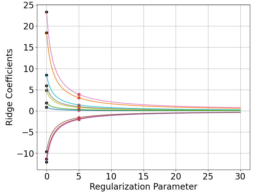
(a) Outcome model

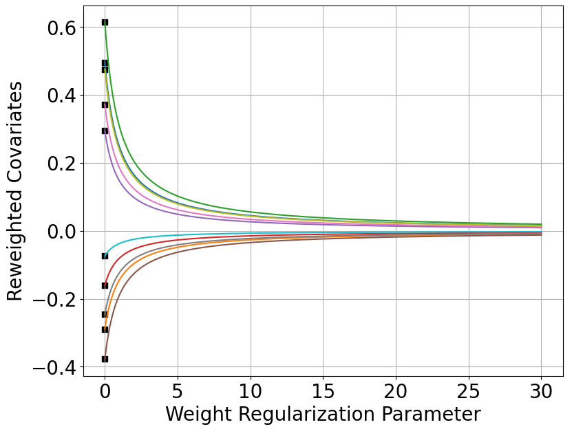
(b) Weighting model

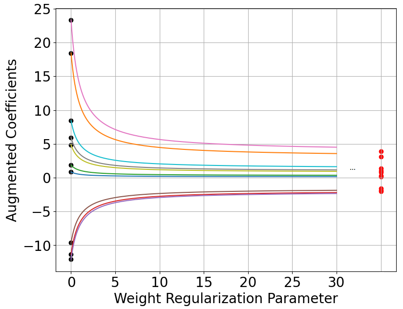
(c) Augmented model

Figure 1: Regularization paths for “double ridge” augmented $\ell_{2}$ balancing weights. Panel (a) shows the coefficients $\hat{\beta}_{\text{reg}}^{\lambda}$ of a ridge regression of $Y_{p}$ on $\Phi_{p}$ with hyperparameter $\lambda$. The black dots on the left are the OLS coefficients, with $\lambda=0$. The red dots at $\lambda=5$ illustrate the coefficients at a plausible hyperparameter value, $\hat{\beta}_{\text{reg}}^{5}$. Panel (b) shows re-weighted covariates, $\hat{\Phi}_{q}^{\delta}$, for the $\ell_{2}$ balancing weights problem with hyperparameter $\delta$; the black dots show exact balance, which corresponds to OLS. As $\delta$ increases, the weights converge to uniform weights and $\hat{\Phi}_{q}^{\delta}$ converges to $\overline{\Phi}_{p}$, which we have centered at zero. Panel (c) shows the augmented coefficients, $\hat{\beta}_{\ell_{2}}$ as a function of the weight regularization parameter $\delta$. The black dots on the left are the OLS coefficients. As $\delta\to\infty$, the coefficients converge to $\hat{\beta}_{\text{reg}}^{5}$. All three regularization paths have essentially identical qualitative behavior.

We can also view $\hat{\beta}_{\ell_{2}}$ as the output of a single iteration of a ridge boosting procedure, fit using $Y_{p}$ and $\Phi_{p}$ alone. See Bühlmann and Yu (2003) and Park et al. (2009) for detailed discussion; Newey et al. (2004) makes a similar connection in the context of twicing kernels.

Proposition 4.2.

Let $\check{Y}_{p}=Y_{p}-\Phi_{p}\hat{\beta}^{\lambda}_{\text{reg}}$ be the residuals from the base learner. Let $\hat{\beta}_{\text{boost}}^{\delta}$ be the coefficients from the ridge regression of $\check{Y}_{p}$ on $\Phi_{p}$ with hyperparameter $\delta$. Then, $\hat{\beta}_{\ell_{2}}=\hat{\beta}_{\text{reg}}^{\lambda}+\hat{\beta}_{\text{boost}}^{\delta},$ and $\|Y_{p}-\Phi_{p}\hat{\beta}_{\ell_{2}}\|_{2}^{2}\leq\|Y_{p}-\Phi_{p}\hat{\beta}_{\text{reg}}^{\lambda}\|_{2}^{2}.$

So for a fixed $\delta$, the augmented $\ell_{2}$ balancing estimator is equivalent to estimating a new outcome model $\hat{\beta}_{\ell_{2}}$ that overfits relative to $\hat{\beta}_{\text{reg}}^{\lambda}$ (in the sense of having smaller in-sample training error), and then applying that model to $\Phi_{q}$.

Surprisingly — and in contrast to the general result in Proposition 3.2 — the augmented coefficients $\hat{\beta}_{\ell_{2}}$ are the same for every target covariate profile $\Phi_{q}$. To see this, note that Proposition 4.1 shows that $\ell_{2}$ balancing weights are always linear in $\mkern 1.5mu\overline{\mkern-1.5mu\Phi\mkern-1.5mu}\mkern 1.5mu_{q}$. Therefore, the corresponding regularization path $a_{j}^{\delta}$ does not depend on the target profile $\Phi_{q}$; it depends only on $\delta$ and the source distribution variances $\sigma_{j}^{2}$. This property is closely related to universal adaptability in the computer science literature on multi-group fairness (Kim et al., 2022b). The particular $\Phi_{q}$ may nonetheless impact the choice of $\delta$ in hyperparameter selection, e.g., via cross-validating imbalance, which in turn influences the degree of overfitting; see Section 7.

4.2 Ridge regression outcome model

Proposition 4.1 holds for arbitrary linear outcome models $\hat{\beta}_{\text{reg}}^{\lambda}\in\mathbb{R}^{d}$; we now state the corresponding result for a “double ridge” estimator, where the base learner outcome model is itself fit via ridge regression. The key takeaway is that the implied augmented coefficients are undersmoothed relative to the base learner ridge coefficients.

For this section, we will consider the following generalized ridge regression, sometimes known as “adaptive” ridge regression (Grandvalet, 1998). Let $\Lambda\in\mathbb{R}^{d\times d}$ be a diagonal matrix with $j$th diagonal entry $\lambda_{j}\geq 0$. Then the generalized ridge coefficients are:

$$\hat{\beta}_{\text{ridge}}^{\Lambda} \coloneqq\underset{\beta\in\mathbb{R}^{d}}{\text{argmin}}\|\Phi_{p}\beta-Y_{p}\|_{2}^{2}+\beta^{\top}\Lambda\beta$$

$$=(\Phi_{p}^{\top}\Phi_{p}+\Lambda)^{-1}\Phi_{p}^{\top}Y_{p}.$$

Standard ridge regression is the special case where the $\lambda_{j}$ all take the same value and so $\Lambda=\lambda I$. As above, the generalized ridge coefficients can be rewritten as shrinking the OLS coefficients:

$$\hat{\beta}_{\text{ridge},j}^{\Lambda}=\left(\frac{\sigma^{2}_{j}}{\sigma^{2}_{j}+\lambda_{j}}\right)\hat{\beta}_{\text{ols},j}.$$ (16)

We now demonstrate that the augmented $\ell_{2}$ balancing weights estimator with base learner $\hat{\beta}_{\text{ridge}}^{\Lambda}$ is equivalent to a plug-in estimator using generalized ridge with smaller hyperparameters, $\hat{\beta}_{\text{ridge}}^{\Gamma}$, where $\Gamma$ is a diagonal matrix with $j$th diagonal entry $\gamma_{j}\in[0,\lambda_{j}]$.

Proposition 4.3.

Let $\hat{\beta}^{\Lambda}_{\text{ridge}}$ denote the coefficients of a generalized ridge regression of $Y_{p}$ on $\Phi_{p}$ with hyperparameters $\Lambda$, and let $\hat{w}^{\delta}_{\ell_{2}}$ denote $\ell_{2}$ balancing weights with hyperparameter $\delta$ defined in Section 2.3. Define the diagonal matrix $\Gamma$ with $j$th diagonal entry:

$$\gamma_{j}\coloneqq\frac{\delta\lambda_{j}}{\sigma_{j}^{2}+\lambda_{j}+\delta}\leq\lambda_{j}.$$

Then:

$$\hat{\mathbb{E}}[\Phi_{q}\hat{\beta}^{\Lambda}_{\text{ridge}}]+\hat{\mathbb{E}}[\hat{w}^{\delta}_{\ell_{2}}(Y_{p}-\Phi_{p}\hat{\beta}^{\Lambda}_{\text{ridge}})]=\hat{\mathbb{E}}[\Phi_{q}\hat{\beta}_{\text{ridge}}^{\Gamma}].$$

Furthermore, $\hat{\beta}_{\text{ridge}}^{\Gamma}$ are standard ridge regression coefficients (i.e., $\gamma_{j}$ is a constant for all $j$) when $\lambda_{j}=\lambda$ and $\sigma_{j}=\sigma$ for all $j$.

The same result holds for kernel ridge regression; see Section B.4.

In this setting, augmenting with balancing weights is equivalent to undersmoothing the original outcome model fit. In particular, we can use the expansion in Equation 16 to see the undersmoothing in $\hat{\beta}^{\Gamma}_{\text{ridge}}$ explicitly:

$$\frac{\sigma^{2}_{j}}{\sigma^{2}_{j}+\gamma_{j}}=\underbrace{\left(\frac{\sigma^{2}_{j}}{\sigma^{2}_{j}+\lambda_{j}}\right)}_{\text{outcome model}}\underbrace{\left(\frac{\sigma_{j}^{2}+\lambda_{j}+\delta}{\sigma_{j}^{2}+\delta}\right)}_{\text{augmentation}},$$

where the first term is the shrinkage from the original generalized ridge model alone, and the second term is due to augmenting with $\ell_{2}$ balancing weights. Importantly, the second term is in $[1,\frac{\sigma^{2}_{j}+\lambda_{j}}{\sigma^{2}_{j}}]$ and therefore partially reverses the shrinkage of the original estimate. In Section 7, we connect this to undersmoothing in the statistical sense.

5 Augmented $\ell_{\infty}$ balancing weights

In this section, we study $\ell_{\infty}$ balancing weights estimators, which are widely used in the balancing weights literature (Zubizarreta, 2015; Athey et al., 2018) and in the AutoDML literature (Chernozhukov et al., 2022d). In the main text, we consider the special case where the covariance matrix $\Phi_{p}^{\top}\Phi_{p}$ is diagonal; that is, $(\Phi_{p}^{\top}\Phi_{p})=\text{diag}(\sigma^{2}_{1},\sigma^{2}_{2},...,\sigma^{2}_{d})$, with $\sigma^{2}_{j}>0$. Unlike with $\ell_{2}$ balancing, this is no longer without loss of generality. We discuss this general case in Section E.3.

For diagonal covariance, we first show that $\ell_{\infty}$ balancing has a closed form: it is equivalent to applying a soft-thresholding operator to the feature shift from $\mkern 1.5mu\overline{\mkern-1.5mu\Phi\mkern-1.5mu}\mkern 1.5mu_{p}$ to $\mkern 1.5mu\overline{\mkern-1.5mu\Phi\mkern-1.5mu}\mkern 1.5mu_{q}$. We then write the resulting augmented estimator as applying coefficients $\hat{\beta}_{\ell_{\infty}}$ to $\Phi_{q}$ and show that $\hat{\beta}_{\ell_{\infty}}$ is a sparse, element-wise convex combination of the base learner coefficients and OLS coefficients. When the outcome model is also fit via the lasso, we use the resulting representation to demonstrate a familiar “double selection” phenomenon (Belloni et al., 2014), where $\hat{\beta}_{\ell_{\infty}}$ inherits the non-zero coefficients of both the base learner and the weighting model. This is a form of undersmoothing in the $\ell_{0}$ “norm,” in the sense that $\hat{\beta}_{\ell_{\infty}}$ always has at least as many non-zero coefficients as the base learner, $\hat{\beta}_{\text{reg}}$.

5.1 Weighting alone

We first define the soft-thresholding operator and show that the $\ell_{\infty}$ balancing problem has a closed form solution.

Definition (Soft-thresholding operator).

For $t>0$, define the soft-thresholding operator,

$$\mathcal{T}_{t}(z)\coloneqq\begin{cases}0&\text{if }|z|<t\\ z-t&\text{if }z>t\\ z+t&\text{if }z<-t\end{cases}.$$

Proposition 5.1 ($\ell_{\infty}$ Balancing).

If $\Phi_{p}^{\top}\Phi_{p}$ is diagonal, the solution $w_{\ell_{\infty}}^{\delta}$ to the $\ell_{\infty}$ optimization problem (11) is:

$$\tfrac{1}{n}w_{\ell_{\infty}}^{\delta} =\Phi_{p}(\Phi_{p}^{\top}\Phi_{p})^{-1}\left[\mkern 1.5mu\overline{\mkern-1.5mu\Phi\mkern-1.5mu}\mkern 1.5mu_{p}+\mathcal{T}_{\delta}(\mkern 1.5mu\overline{\mkern-1.5mu\Phi\mkern-1.5mu}\mkern 1.5mu_{q}-\mkern 1.5mu\overline{\mkern-1.5mu\Phi\mkern-1.5mu}\mkern 1.5mu_{p})\right]$$

$$=\Phi_{p}(\Phi_{p}^{\top}\Phi_{p})^{-1}\left[\mkern 1.5mu\overline{\mkern-1.5mu\Phi\mkern-1.5mu}\mkern 1.5mu_{p}+\mathcal{T}_{\delta}(\Delta)\right]$$

where $\Delta=\mkern 1.5mu\overline{\mkern-1.5mu\Phi\mkern-1.5mu}\mkern 1.5mu_{q}-\mkern 1.5mu\overline{\mkern-1.5mu\Phi\mkern-1.5mu}\mkern 1.5mu_{p}$, where we include $\mkern 1.5mu\overline{\mkern-1.5mu\Phi\mkern-1.5mu}\mkern 1.5mu_{p}$ (equal to $0$ by assumption) to emphasize the dependence on feature shift, and with corresponding reweighted features, $\hat{\Phi}_{q}^{\delta}=\mkern 1.5mu\overline{\mkern-1.5mu\Phi\mkern-1.5mu}\mkern 1.5mu_{p}+\mathcal{T}_{\delta}(\mkern 1.5mu\overline{\mkern-1.5mu\Phi\mkern-1.5mu}\mkern 1.5mu_{q}-\mkern 1.5mu\overline{\mkern-1.5mu\Phi\mkern-1.5mu}\mkern 1.5mu_{p})$.

For intuition, compare the (un-augmented) $\ell_{\infty}$ balancing weights estimator to the lasso coefficients (Hastie et al., 2009):

$$\hat{\mathbb{E}}[w_{\ell_{\infty}}^{\delta}\circ Y_{p}] =\mathcal{T}_{\delta}(\mkern 1.5mu\overline{\mkern-1.5mu\Phi\mkern-1.5mu}\mkern 1.5mu_{q})^{\top}\hat{\beta}_{\text{ols}}$$

$$\hat{\mathbb{E}}[\Phi_{q}\hat{\beta}_{\text{lasso}}^{\lambda}] =\mkern 1.5mu\overline{\mkern-1.5mu\Phi\mkern-1.5mu}\mkern 1.5mu_{q}^{\top}\mathcal{T}_{\lambda}(\hat{\beta}_{\text{ols}}),$$

where we simplify $\hat{\Phi}_{q}^{\delta}$ here to emphasize the connections between the methods. Whereas lasso performs soft-thresholding on the OLS coefficients (regularizing the outcome regression), $\ell_{\infty}$ balancing performs soft-thresholding on the implied feature shift to the target features.

5.2 General linear outcome model

We can then plug the closed-form solution for the weights into Proposition 3.2.

Proposition 5.2.

Let $\hat{w}_{\ell_{\infty}}^{\delta}$ be defined as above. Then the augmented $\ell_{\infty}$ balancing weights estimator with outcome model fit $\hat{\beta}_{\text{reg}}^{\lambda}\in\mathbb{R}^{d}$ has the form,

$$\hat{\mathbb{E}}[\Phi_{q}\hat{\beta}_{\text{reg}}^{\lambda}]+\hat{\mathbb{E}}[\hat{w}_{\ell_{\infty}}^{\delta}(Y_{p}-\Phi_{p}\hat{\beta}_{\text{reg}}^{\lambda})]=\hat{\mathbb{E}}[\Phi_{q}\hat{\beta}_{\ell_{\infty}}],$$

where the $jth$ coefficient of $\hat{\beta}_{\ell_{\infty}}$ equals:

$$\hat{\beta}_{\ell_{\infty},j}=\begin{cases}\hat{\beta}_{\text{reg},j}^{\lambda}&\text{if }|\Delta_{j}|<\delta\\[5.0pt] \left|\frac{\delta}{\Delta_{j}}\right|\hat{\beta}_{\text{reg},j}^{\lambda}+\left(1-\left|\frac{\delta}{\Delta_{j}}\right|\right)\hat{\beta}_{\text{ols},j}&\text{otherwise}\\ \end{cases},$$

where $\Delta_{j}=\mkern 1.5mu\overline{\mkern-1.5mu\Phi\mkern-1.5mu}\mkern 1.5mu_{q,j}-\mkern 1.5mu\overline{\mkern-1.5mu\Phi\mkern-1.5mu}\mkern 1.5mu_{p,j}$.

The augmented coefficients $\hat{\beta}_{\ell_{\infty}}$ are an element-wise convex combination of $\hat{\beta}_{\text{reg}}^{\lambda}$ and $\hat{\beta}_{\text{ols}}$. For features where the mean feature shift $\Delta_{j}$ is small (relative to $\delta$), $\hat{\beta}_{\ell_{\infty}}$ is equivalent to the base learner coefficient $\hat{\beta}_{\text{reg}}^{\lambda}$. The remaining coefficients are interpolated linearly toward the $\hat{\beta}_{\text{ols}}$ coefficients.

Figure 2 summarizes these results and their implications for the augmented estimator. As with Figure 1, we generate simple simulated data with $d=10$. In the left panel, we plot the coefficients from lasso regression of $Y_{p}$ on $\Phi_{p}$ as a function of the lasso regularization parameter. The regularization path begins with the black dots, which represent the OLS coefficients. Each lasso coefficient (represented by a colored line) then shrinks linearly to exactly zero, due to the soft-thresholding operator. The middle panel plots the reweighted covariates using $\ell_{\infty}$ balancing weights between $\Phi_{p}$ and $\Phi_{q}$ solved in the constrained form. The black dots represent $\mkern 1.5mu\overline{\mkern-1.5mu\Phi\mkern-1.5mu}\mkern 1.5mu_{q}$, corresponding to exact balance. Then as the weight regularization parameter increases, the reweighted covariates shrink linearly to exactly zero, just as in lasso. The right panel plots coefficients for the augmented estimator that combines a baseline outcome model fit $\hat{\beta}_{\text{reg}}^{\lambda}$ with $\ell_{\infty}$ balancing weights. The lines correspond to $\hat{\beta}_{\ell_{\infty}}$ as defined in Proposition 5.2. The regularization path begins at the black dots, where $\hat{\beta}_{\ell_{\infty}}=\hat{\beta}_{\text{ols}}$, and eventually converges to $\hat{\beta}_{\text{reg}}^{\lambda}$, showing the usual soft-thresholding behavior. The order at which the coefficients go to zero reflects the size of $\mkern 1.5mu\overline{\mkern-1.5mu\Phi\mkern-1.5mu}\mkern 1.5mu_{q}$, because the regularization path depends on the weight coefficients from the middle panel. Thus, the augmented estimator shrinks $\hat{\beta}_{\text{ols}}$ toward $\hat{\beta}_{\text{reg}}^{\lambda}$ but via a soft-thresholding operator applied to the feature shift, $\Delta_{j}$.

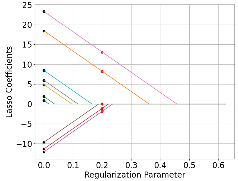
(a) Outcome model

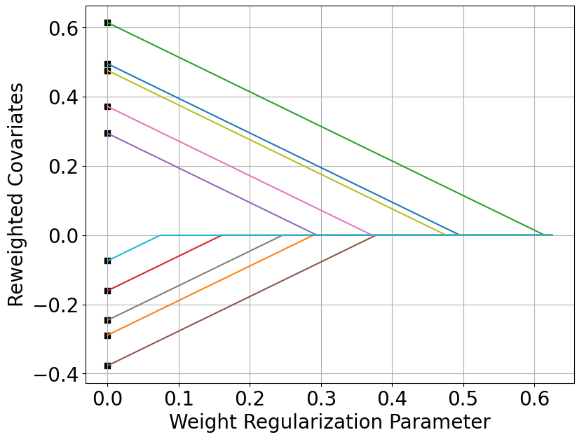
(b) Weighting model

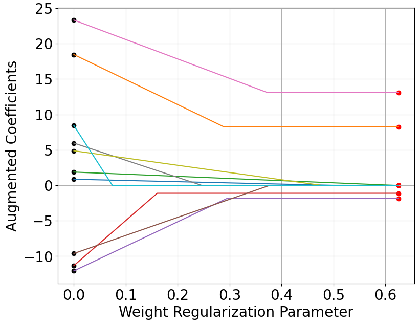
(c) Augmented model

Figure 2: Regularization paths for “double lasso” augmented $\ell_{\infty}$ balancing weights. Panel (a) shows the coefficients $\hat{\beta}_{\text{reg}}^{\lambda}$ of a lasso regression of $Y_{p}$ on $\Phi_{p}$ with hyperparameter $\lambda$. The black dots on the left are the OLS coefficients, with $\lambda=0$. The red dots at $\lambda=0.2$ illustrate the coefficients at a plausible hyperparameter value, $\hat{\beta}_{\text{reg}}^{0.2}$. Panel (b) shows re-weighted covariates, $\hat{\Phi}_{q}^{\delta}$, for the $\ell_{\infty}$ balancing weights problem with hyperparameter $\delta$; the black dots show exact balance, which corresponds to OLS. As $\delta$ increases, the weights converge to uniform weights and $\hat{\Phi}_{q}^{\delta}$ converges to $\overline{\Phi}_{p}$, which we have centered at zero. Panel (c) shows the augmented coefficients, $\hat{\beta}_{\ell_{\infty}}$ as a function of the weight regularization parameter $\delta$. The black dots on the left are the OLS coefficients. As $\delta\to\infty$, the coefficients converge to $\hat{\beta}_{\text{reg}}^{0.2}$. All three regularization paths show the typical lasso “soft thresholding” behavior. The regularization path for the augmented estimator also shows “double selection” behavior.

5.3 Lasso outcome model

In the case where $\hat{\beta}_{\text{reg}}^{\lambda}$ is itself fit via lasso, as studied in Chernozhukov et al. (2022d), then we recover a familiar double selection phenomenon (Belloni et al., 2014).

Proposition 5.3 (Double Selection).

Let $\hat{\beta}_{\text{lasso}}^{\lambda}$ denote the coefficients of lasso regression of $Y_{p}$ on $\Phi_{p}$ with regularization parameter $\lambda$. Denote the indices of the non-zero coefficients as $I_{\lambda}$. Let $\hat{w}_{\ell_{\infty}}^{\delta}$ be $\ell_{\infty}$ balancing weights with parameter $\delta$ as in Proposition 5.1. Let $I_{\delta}$ denote the non-zero entries of the reweighted covariates $\hat{\Phi}_{q}$. Assume that $\hat{\beta}_{\text{ols}}$ is dense. Then the indices of the non-zero entries of the augmented coefficients $\hat{\beta}_{\ell_{\infty}}$ are $I_{\text{aug}}=I_{\lambda}\cup I_{\delta}.$

The lasso coefficients have a sparsity pattern generated by soft-thresholding the OLS coefficients. The augmented estimator then shrinks from OLS toward $\hat{\beta}_{\text{reg}}^{\lambda}$ by soft-thresholding the implied feature shift to the target features. As a result, wherever the lasso coefficients are non-zero or the weight coefficients are non-zero, the final augmented coefficients are also non-zero. The “included coefficients” for the final estimator are then the union of the coefficients included in either individual model. Therefore, augmenting a lasso outcome model with $\ell_{\infty}$ balancing also exhibits a form of undersmoothing in the $\ell_{0}$ “norm”, $\|\hat{\beta}_{\ell_{\infty}}\|_{0}$, in the sense that there are always at least as many non-zero coefficients as for the unaugmented lasso outcome model. However, this will not correspond to undersmoothing the base learner in the traditional sense, because in general there will not exist a lasso hyperparameter $\lambda$ that will produce sparsity pattern $I_{\text{aug}}$.

6 Numerical illustrations

We now illustrate these findings through several real-data examples. Following Chernozhukov et al. (2022d), we focus on the canonical LaLonde (1986) data set evaluating a job training program in the National Supported Work (NSW) Demonstration. The primary outcome of interest is annual earnings in 1978 dollars.

For these illustrations, we focus on estimating the Average Treatment Effect on the Treated (ATT), $\mathbb{E}[Y(1)-Y(0)\mid Z=1]$. We recover the missing conditional mean $\mathbb{E}[Y(0)\mid Z=1]$ using the setup from Example 3, where the source and target populations are the control and treated units respectively. Thus $\Phi_{p}$ and $\Phi_{q}$ correspond to the feature expansion $\phi(X)$ applied to the covariates in the control group and treated group respectively. We consider two different features expansions of the original covariates: (1) a “short” set of 11 covariates used in Dehejia and Wahba (1999); and (2) an expanded, “long” set of 171 interacted features used in Farrell (2015).

For the “short” feature set, we show that off-the-shelf augmented balancing weight estimators indeed collapse to simple OLS: for both ridge-augmented $\ell_{2}$ balancing and lasso-augmented $\ell_{\infty}$ balancing, choosing the optimal hyperparameters via cross-validation leads to estimators that are equivalent to OLS. For the expanded feature set, these estimators no longer collapse to OLS. Instead, we show how these estimators undersmooth in practice. For the special case of double ridge, we show that this is equivalent to undersmoothing the hyperparameter in a single ridge regression. We assess the sensitivity of these numerical results to cross-fitting in Section F.2. See Appendix F for dataset summaries and corroborating results from the Infant Health Development Program (IHDP).

6.1 Low-dimensional setting

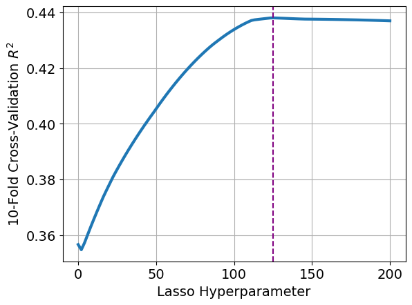
(a) Lasso outcome model

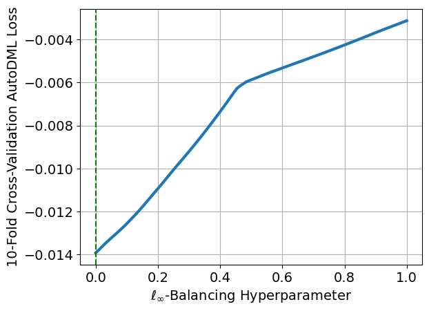
(b) $\ell_{\infty}$ balancing

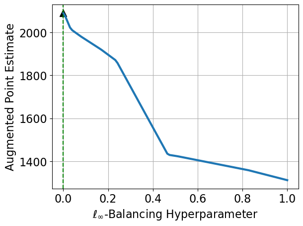
(c) Augmented estimate

Figure 3: Lasso-augmented $\ell_{\infty}$ balancing weights (“double lasso”) for LaLonde (1986) with the original 11 covariates. Panel (a) shows the 10-fold cross-validated $R^{2}$ for the Lasso-penalized regression of $Y_{p}$ on $\Phi_{p}$ among control units across the hyperparameter $\lambda$; the purple dotted line shows the CV-optimal value. Panel (b) shows the 10-fold cross-validated AutoDML loss (8) for $\ell_{\infty}$ balancing weights across the hyperparameter $\delta$; the green dotted line shows the CV-optimal value, which is $\delta=0$ or exact balance. Panel (c) shows the point estimate for the augmented estimator across the weighting hyperparameter $\delta$; the black triangle corresponds to the OLS point estimate, which is also the CV-optimal value based on cross-validating the AutoDML loss.

We begin by applying lasso-augmented $\ell_{\infty}$ balancing weights (“double lasso”) to the short version of the LaLonde (1986) data set with 11 features. The key takeaway is that the resulting estimate collapses to a simple OLS regression, even though the base learner lasso outcome model is heavily regularized. This finding repeats in a variety of low-dimensional settings. Additional results in Section F.3 show the same pattern on Lalonde with $\ell_{2}$ balancing weights, as well as in a re-analysis of the “low-dimensional” IHDP data set with both $\ell_{\infty}$ and $\ell_{2}$ augmented balancing weights.

Figures 3(a) and 3(b) show the cross-validation curves for the outcome and weighting models, respectively. For the outcome model, ten-fold cross-validation chooses a non-zero value for the lasso hyperparameter (purple dotted line) resulting in a sparse model. For the weighting model, however, cross-validation on the automatic form loss function (8) selects the hyperparameter $\delta=0$, which is equivalent to exact balance.

Figure 3(c) shows the point estimate as a function of the weighting hyperparamter $\delta$, holding the outcome model hyperparameter $\lambda$ fixed; the black triangle represents the OLS plug-in point estimate. For context, the corresponding experimental estimate is $1,794 (see Dehejia and Wahba, 1999). Because cross-validation chooses $\delta=0$, the weights achieve exact balance, and $\hat{\beta}_{\text{aug}}=\hat{\beta}_{\text{ols}}$. In short, because the bias-variance trade-off for the weights prefers exact balance, the entire estimator collapses to the simple OLS plug-in estimate, even though our base learner is a highly regularized sparse model.

Some augmented balancing weights procedures, including Chernozhukov et al. (2018), additionally implement sample splitting and cross-fitting. We repeat the numerical experiments in the low-dimensional setting with 5-fold cross-fitting and find that on average (over draws of folds) the estimate is essentially identical to the OLS plug-in estimate, but the distribution is skewed and displays substantial variation. See Section F.2 for a summary of the results.

6.2 High-dimensional setting

We next consider the expanded set of 171 features for LaLonde (1986) used in Farrell (2015). To simplify exposition, we first run a pre-processing step for this expanded feature set using the eigenvectors of $\Phi_{p}^{\top}\Phi_{p}$ to decorrelate the features; as we discuss above, this is without loss of generality for $\ell_{2}$ balancing but not for $\ell_{\infty}$ balancing.

Figure 4 shows estimates for ridge-augmented $\ell_{2}$ balancing (top row) and lasso-augmented $\ell_{\infty}$ balancing (bottom row). The left two panels of each row show the cross-validation curves for the outcome regression and balancing weights, respectively. Unlike in the low-dimensional setting, the CV-optimal hyperparameter is non-zero for all of these models. As a result, the final augmented estimates shown on the right — where the dotted green lines and blue lines intersect in Figure 4(c) and Figure 4(f) — are not equivalent to OLS.

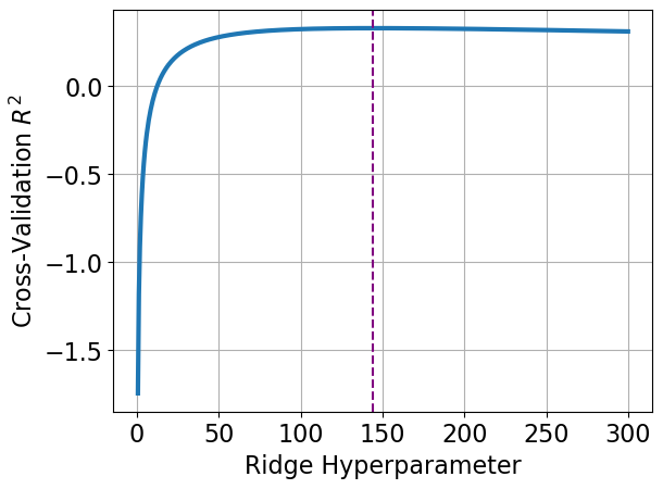
(a) Ridge outcome model

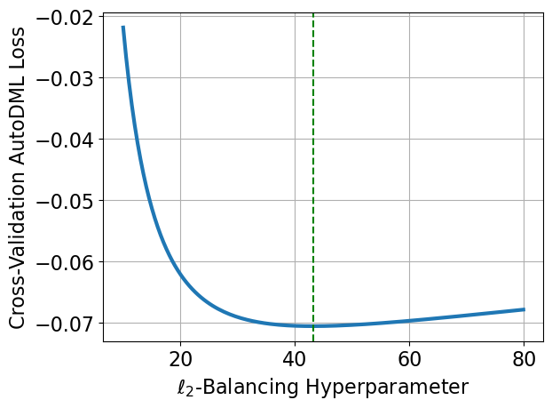
(b) $\ell_{2}$ balancing

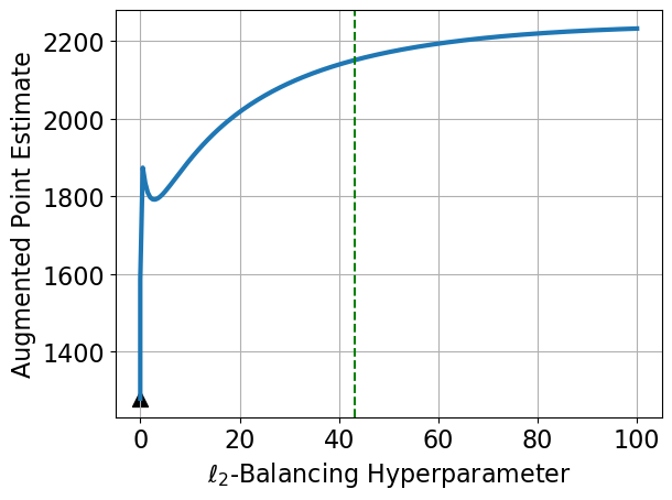
(c) Estimate from “double ridge”

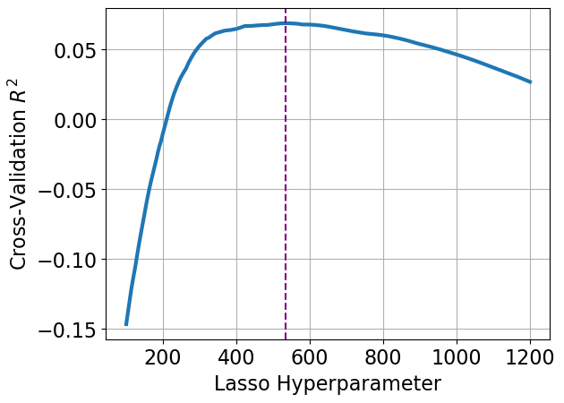
(d) Lasso outcome model

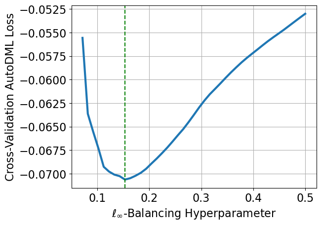
(e) $\ell_{\infty}$ balancing

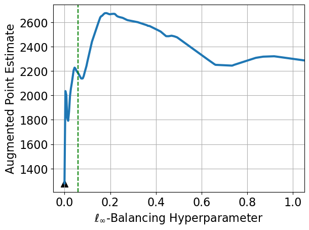
(f) Estimate from “double lasso”

Figure 4: Augmented balancing weights estimates for the LaLonde (1986) data set with the expanded set of 171 features used in Farrell (2015); the top row shows ridge-augmented $\ell_{2}$ balancing, and the bottom row shows lasso-augmented $\ell_{\infty}$ balancing. Panels (a) and (d) show the 3-fold cross-validated $R^{2}$ for the ridge- and laso-penalized regression of $Y_{p}$ on $\Phi_{p}$ among control units across the hyperparameter $\lambda$; the purple dotted lines show the CV-optimal value for each. Panel (b) and (e) show the 3-fold cross-validated AutoDML loss (8) for $\ell_{2}$ and $\ell_{\infty}$ balancing weights across the hyperparameter $\delta$; the green dotted lines show the CV-optimal value for each. Panels (c) and (f) show the point estimates for the augmented estimators across the weighting hyperparameter $\delta$; the black triangles correspond to the OLS point estimate, and the green dotted lines show the CV-optimal value of $\delta$ for each.

6.2.1 Undersmoothing for double ridge

For the special case of double ridge, we now illustrate our result from Proposition 4.3 that $\ell_{2}$ balancing weights produce a new outcome model that is undersmoothed relative to the original ridge regression model. Recall that when the base learner is a generalized ridge model with parameters $\lambda_{j}$, then the augmented estimator is equivalent to plugging in a generalized ridge models with parameters $\gamma_{j}\leq\lambda_{j}$. In this example, the $\lambda_{j}$ are all equal to the same value (chosen via cross-validation), indicated by the purple dotted line in Figure 4(a). We compute the corresponding $\gamma_{j}$ for $\delta$ chosen by cross-validation, indicated by the green dotted line in Figure 4(b).

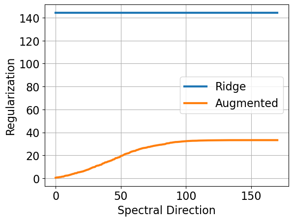
(a) Adaptive regularization

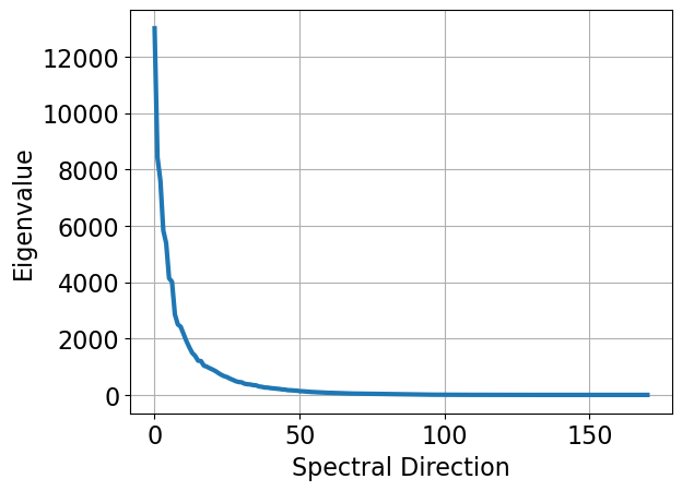
(b) Eigenvalues of $\Phi_{p}^{\top}\Phi_{p}$

Figure 5: Single and double ridge regression applied to the “high-dimensional” version of the LaLonde (1986) data set. Panel (a) shows $\lambda_{j}$, the single ridge hyperparameter, and $\gamma_{j}$, the implied double ridge hyperparameter, as functions of the spectral direction $j$. Panel (b) shows the corresponding eigenvalues.

Figure 5(a) plots the $\lambda_{j}$ and $\gamma_{j}$, with $j$ on the $x$-axis sorted in the order of the eigenvalues of $\Phi_{p}^{\top}\Phi_{p}$ from largest to smallest. Figure 5(b) plots the corresponding eigenvalues. For standard ridge regression, the key idea is to push the eigenvalues of $\Phi_{p}^{\top}\Phi_{p}$ away from zero so that the resulting matrix $\Phi_{p}^{\top}\Phi_{p}+\lambda I$ is invertible and well-conditioned. Thus, the original ridge regression applies the same amount of regularization across the spectrum, as shown by the blue line in Figure 5(a). By contrast, the implied outcome model from the augmented procedure uses far less regularization and is substantially undersmoothed. Importantly, the augmented estimator undersmooths more where the eigenvalues of $\Phi_{p}^{\top}\Phi_{p}$ are large and undersmooths less where the eigenvalues of $\Phi_{p}^{\top}\Phi_{p}$ are close to zero. The augmented estimator therefore avoids bias by only regularizing the spectral directions that are the most significant sources of variation — and even these to a much smaller degree than is optimal for MSE predictions.

6.2.2 Undersmoothing in norm

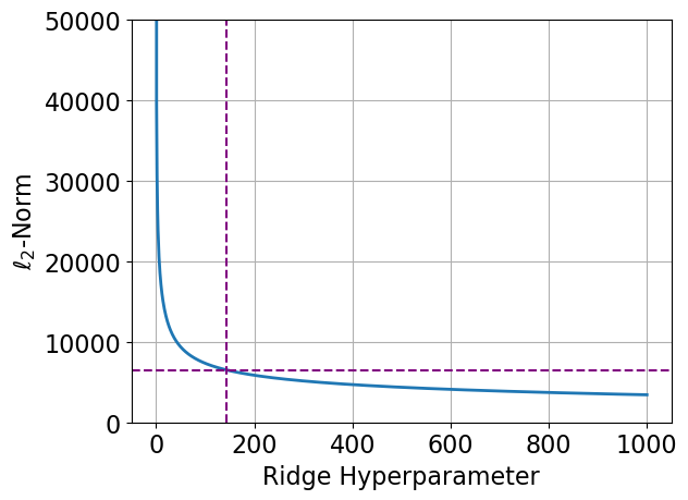
(a) $\ell_{2}$ norm for ridge outcome model

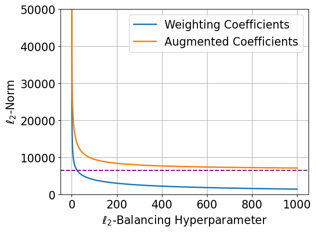
(b) $\ell_{2}$ norm for weighting and double ridge

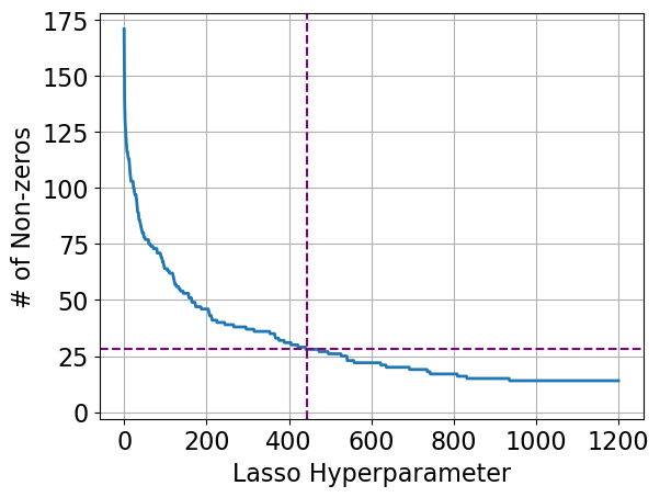
(c) $\ell_{0}$ “norm” for lasso outcome model

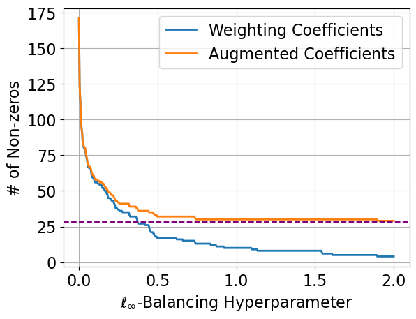
(d) $\ell_{0}$ “norm” for weighting and double lasso

Figure 6: Undersmoothing in norms for augmented balancing weights applied to the “high dimesional” version of the LaLonde (1986) data set. Panels (a) and (c) show the $\ell_{2}$ norm and the number of non-zero covariates (the $\ell_{0}$ “norm”) for the ridge and lasso regression, respectively, of $Y_{p}$ on $\Phi_{p}$ among control units. Panels (b) and (d) show the $\ell_{2}$ and number of non-zero covariates for the corresponding unaugmented and augmented balancing weights estimators. The dotted purple line is the outcome model hyperparameter chosen via cross validation. The norms for the augmented estimators are always at least as large as for the outcome model alone.

For the special case with diagonal covariates, both double ridge and double lasso undersmooth in a particular norm of $\|\hat{\beta}_{\text{aug}}\|$, relative to the unaugmented outcome model, as shown in Figure 6. In particular, Figures 6(a) and 6(c) show the $\ell_{2}$ norm and the number of included covariates (the $\ell_{0}$ “norm”) for the ridge and lasso outcome regression models, respectively, as a function of the outcome hyperparameter $\lambda$. The purple dotted lines show the values of $\lambda$ chosen via cross validation, and the corresponding values of the $\ell_{2}$ and $\ell_{0}$ norms. Figures 6(b) and 6(d) show the corresponding norm for the unaugmented and balancing weights estimators, “double ridge” and “double lasso,” respectively. For both, the norms for the augmented estimators are always at least as large as the norms for the outcome model alone. While the patterns are qualitatively the same, the behavior for $\ell_{\infty}$ balancing does not correspond to traditional undersmoothing, since the union of non-zero coefficients of the outcome and weighting models cannot generally be recovered by changing the hyperparameter of the lasso outcome model.

7 Undersmoothing and asymptotic results for kernel ridge regression

Our numeric results above suggests a way to understand augmented balancing weights through the lens of undersmoothing — and vice versa. In particular, we show above that ridge-augmented $\ell_{2}$ balancing is numerically equivalent to a single, undersmoothed (generalized) ridge regression outcome model, and that this equivalence holds for kernel ridge regression. We now show that these numerical results extend to undersmoothing in the statistical sense as well.

7.1 Regularization bias, double robustness, and undersmoothing

Using off-the-shelf penalized regression leads to non-negligible regularization bias for our target estimand: choosing the hyperparameter that minimizes the predictive MSE does not drive the bias to zero sufficiently fast asymptotically. Undersmoothing — choosing a smaller regularization parameter than is prediction optimal — is an alternative to the doubly robust approach of using an augmentation term as a bias correction (Goldstein and Messer, 1992; Newey et al., 1998). A main difficulty lies in finding the optimal hyperparameter.

A series of recent papers have explored both approaches in the context of kernel ridge regression. From the doubly robust perspective, Wong and Chan (2018) and Singh (2021) show that forms of “double kernel ridge” are semiparametrically efficient. From the undersmoothing perspective, Hirshberg et al. (2019) and Mou et al. (2023) demonstrate that a single, unaugmented kernel ridge regression estimator can also achieve efficiency with careful selection of the regularization schedule.

Our Proposition 4.3 demonstrates that the augmented balancing weights estimator in the RKHS setting with “double kernel ridge regression” is numerically equivalent to a single-stage undersmoothed kernel ridge estimator. To relate the existing statistical analyses, we will begin with the RKHS framework in Caponnetto and De Vito (2007) and derive the implied undersmoothed kernel ridge hyperparameter of the corresponding augmented estimator from Singh (2021). We find that the implied hyperparameter can go to zero either faster or slower than the standard rate of $n^{-1}$ studied in the undersmoothing literature, depending on the effective dimension and smoothness of the outcome model in the RKHS.

7.2 The statistical setting

To move from numerical results to statistical results, we must place some constraints on the data generating process. Our setup for the RKHS follows Singh (2021). First, assume that the space $\mathcal{X}\times\mathcal{Z}$ is Polish. Let $\mathcal{H}$ be an RKHS on $\mathcal{X}\times\mathcal{Z}$ with corresponding kernel $k$ satisfying standard regularity conditions (Singh, 2021, Assumption 5.2) and let $\eta_{j}$, $\varphi_{j}$ denote the eigenvalues and eigenfunctions respectively of its kernel integral operator under $p$. Next, assume that the eigenvalues satisfy the decay condition $\eta_{j}\leq Cj^{-b}$ for some $b>1$ and a constant $C$. The parameter $b$ encodes information on the effective dimension of $\mathcal{H}$. For a bounded kernel, $b>1$ (Fischer and Steinwart, 2020): the case where $b=\infty$ corresponds to a finite-dimensional RKHS; for the case with $1<b<\infty$, the $\eta_{j}$ must decay at a polynomial rate.

We then assume that for some $c\in[1,2]$, the outcome function $m(x,z)$ belongs to the set:

$$\mathcal{H}^{c}\coloneqq\left\{f=\sum^{\infty}_{j=1}a_{j}\varphi_{j}:\sum^{\infty}_{j=1}\frac{a_{j}^{2}}{\eta^{c}_{j}}<\infty\right\}\subset\mathcal{H},$$ (17)

where $c$ encodes additional smoothness of the conditional expectation. If $c=1$, then by the spectral decomposition of the RKHS, Equation 17 is equivalent to requiring $m\in\mathcal{H}$; choosing larger values of $c$ corresponds to $m$ being a smoother element of $\mathcal{H}$, with a “saturation effect” kicking in for $c>2$ (Bauer et al., 2007). Varying $b$ (the effective dimension of the RKHS) and $c$ (the additional smoothness of the outcome function) changes the optimal rates for regression, with larger values of both corresponding to faster rates of convergence.

Finally, we assume that the Riesz representer, $\alpha(x,z)$, of our linear functional estimand also belongs to $\mathcal{H}^{c}$. Under these conditions, Singh (2021) demonstrates that an augmented estimator combining kernel balancing weights and a kernel ridge regression base learner is asymptotically normal. Furthermore, it follows that the asymptotic variance achieves the semiparametric efficiency bound. Now we will demonstrate a setting where this estimator is equivalent to a single undersmoothed kernel ridge regression.

7.3 Implied undersmoothing for kernel ridge regression

Under the conditions outlined above, assume that we observe $n$ iid samples of $(x_{i},y_{i},z_{i})$ from $p$. Define $K\in\mathbb{R}^{n\times n}$ to be the kernel matrix with $i,j$-th entry $K_{ij}=k((x_{i},z_{i}),(x_{j},z_{j}))$. Let $\sigma_{j}^{2}$ denote the eigenvalues of $K$ and assume that $\sigma_{j}^{2}=\sigma^{2}$, a constant for all $j$. The kernel ridge regression outcome model with parameter $\lambda$ has coefficients:

$$\hat{\beta}_{\text{ridge}}^{\lambda}=(K+\lambda I)^{-1}y.$$

Applying Proposition 4.3, the augmented estimator with hyperparameter $\delta$ is equivalent to a plug-in estimate with a new kernel ridge model:

$$\hat{\beta}_{\text{aug}}=(K+\gamma I)^{-1}y,$$

with hyperparameter

$$\gamma=\frac{\lambda\delta}{\sigma^{2}+\lambda+\delta}.$$

Following Caponnetto and De Vito (2007), Theorems 5.1 and 5.2 of Singh (2021) use hyperparameter schedules for $\lambda$ and $\delta$, which depend on the effective dimension $b$ and smoothness $c$:

$$\lambda_{n}=\delta_{n}=\begin{cases}n^{-1/2}&\textrm{ if }b=\infty\\ n^{-\frac{b}{bc+1}}&\textrm{ if }b\in(1,\infty),\quad c\in(1,2]\\ (n/\log(n))^{-b/(b+1)}&\textrm{ if }b\in(1,\infty),\quad c=1\end{cases},$$

For two functions of $n$, $f_{n}$ and $g_{n}$, let $f_{n}\asymp g_{n}$ denote that $f_{n}=O(g_{n})$ and $g_{n}=O(f_{n})$. We can compute the implied augmented hyperparameter $\gamma$ (for large $n$) using the following proposition.

Proposition 7.1.

Let $\lambda_{n}>0$ be any monotonically decreasing function of $n$ and let $\delta_{n}=\lambda_{n}$. Then:

$$\gamma_{n}\coloneqq\frac{\lambda_{n}\delta_{n}}{\sigma^{2}+\lambda_{n}+\delta_{n}}\asymp\lambda_{n}^{2}.$$

To see the connection between double kernel ridge regression and undersmoothing, first consider the standard ridge regression case, which corresponds to the finite-dimensional setting with $b=\infty$. Here, we choose hyperparameter $\lambda_{n}=\delta_{n}=n^{-1/2}$ to control the prediction error for both the outcome and weighting models. The augmented estimator is then equivalent to a single ridge regression with hyperparameter $\gamma_{n}\asymp n^{-1}$. Hence, this will always undersmooth relative to the MSE-optimal hyperparameter for a single ridge regression.

This rate matches the one typically used in undersmoothed kernel ridge regression analyses. For example, both Hirshberg et al. (2019) and Mou et al. (2023) demonstrate that, in a similar statistical setting, plug-in estimators of linear functionals using kernel ridge regression with a hyperparameter schedule of $\lambda_{n}\asymp n^{-1}$ can be semiparametrically efficient.

The optimal undersmoothing analysis from Hirshberg et al. (2019) and Mou et al. (2023) also extends to the infinite-dimensional setting ($b<\infty$). By contrast, we find that the undersmoothed hyperparameter implied by the augmented procedure can take on a range of asymptotic rates, both faster and slower than $n^{-1}$, in this infinite-dimensional setting. The implied augmented hyperparameter is of order $\lambda_{n}^{2}$ and the MSE-optimal hyperparameter schedules for the base learner, $\lambda_{n}$, can be faster or slower than $n^{-1/2}$ depending on the effective dimension $b$ and smoothness $c$ of the RKHS.

For example, when $c>1$, the optimal rate for $\lambda_{n}$ is $n^{-\frac{b}{bc+1}}$; the implied hyperparameter is then order $n^{-2b/bc+1}\in(n^{-2},n^{-2/3})$ for $c\in(1,2]$ and $b\in(1,\infty)$. Whether or not this smooths more than $n^{-1}$ therefore depends on the relationship between the effective dimension $b$ and the smoothness $c$. In particular, the implied hyperparameter goes to zero at a slower rate than $n^{-1}$ whenever $c\geq 2-\frac{1}{b}$. In this sense, Proposition 7.1 generalizes the standard undersmoothing arguments, which typically shift the regularization schedule from $n^{-1/2}$ to $n^{-1}$. It is unclear whether the rates we find here are the only undersmoothed rates that will yield efficiency for fixed $b$ and $c$; we leave a thorough investigation to future work.

The results thus far are inherently theoretical, as they depend on unknown properties of the underlying RKHS and outcome function. Thus, we view this more as an aid to understanding rather than giving practical guidance. However, one simple heuristic suggested by Proposition 7.1 is to choose $\lambda_{n}$ by standard cross-validation and then use a single-stage kernel ridge regression estimator with hyperparameter $\lambda_{n}^{2}$ (as long as the cross-validated $\lambda_{n}$ is smaller than $1$). This assumes that the cross-validated $\lambda_{n}$ is rate-optimal and we leave an empirical investigation of practical performance to future work. Finally, we note that these results are unique to $\ell_{2}$ balancing and, especially, do not appear to hold for $\ell_{\infty}$ balancing weights.

8 Discussion

We have shown that augmenting a plug-in regression estimator with linear balancing weights results in a new plug-in estimator with coefficients that are shrunk towards — in some cases all the way to — the estimates from OLS fit on the same observations. We generalize this equivalence for different choices of outcome and weighting regressions, and connect this to undersmoothing for the special case of kernel ridge regression. We then illustrate these results on a canonical data set, highlighting the role of modeling choices and hyperparameter tuning. In the Appendix also explore many extensions, including to nonlinear weights and to high-dimensional features.

There are many promising avenues for future research. The fundamental connection between doubly robust estimation undersmoothing opens up several theory directions. While we focus on the special case of kernel ridge regression in Section 7, we anticipate that these connections will hold more broadly. Similarly, while our focus in this paper has been on interpreting balancing weights as a form of linear regression, the converse is also valid: we could instead focus on how many outcome regression-based plug-in estimators are, in fact, a form of balancing weights; see Lin and Han (2022) for connections between outcome modeling and density ratio estimation.

We also anticipate that our numeric results will lead to better guidance for deploying augmented balancing weights in practice. The most immediate question is hyperparameter tuning, for which recommendations vary (e.g., Kallus, 2020; Wang and Zubizarreta, 2020; Chernozhukov et al., 2022d). We expect that the connection to theoretically optimal results for undersmoothing (e.g., Mou et al., 2023) can help guide hyperparameter choice in the settings where we have shown augmented estimators to be equivalent to undersmoothed outcome regression. More broadly, we can consider special cases, such as multivariate Gaussians, for which we can reason about trade-offs for different choices.

We conjecture that these results may provide new insights into the estimation of causal effects in the proximal causal inference framework (Tchetgen Tchetgen et al., 2020). This framework uses proxy variables to identify causal effects in the presence of unmeasured confounding. Estimation has been complicated by the fact that, in the absence of strong parametic assumptions, estimators of proximal causal effects are solutions to ill-posed Fredholm integral equations. Ghassami et al. (2022) and Kallus et al. (2021) recently proposed tractable nonparametric estimators in this setting. They use an “adversarial” version of double kernel ridge regression — allowing the weighting and outcome models to have different bases — to estimate the solution to the required Fredholm integral equations. Our results apply immediately to standard augmented estimators with different bases for the outcome and weighting models, either via a union basis (Chernozhukov et al., 2022d) or by applying an appropriate projection as in Hirshberg and Wager (2021), and extending these results to proximal causal effect estimators might help in constructing new proximal balancing weights, matching, or regression estimators with attractive asymptotic properties.

Finally, many common panel data estimators are forms of augmented balancing weight estimation (Abadie et al., 2010; Ben-Michael et al., 2021c; Arkhangelsky et al., 2021). We plan to use the numeric results here, especially the results for simplex-constrained weights in Appendix D.2, to better understand connections between methods and to inform inference.

Appendix A Equivalences of outcome regression and balancing weighting methods

For the special case of $\ell_{2}$ kernel balancing, the balancing weights problem is numerically equivalent to directly estimating the conditional expectation $\mathbb{E}[Y_{p}|\Phi_{p}]$ via kernel ridge regression and applying the estimated coefficients to $\bar{\Phi}_{q}$. We begin with the special case of unregularized linear regression and then present the more general setting. We initially present the results assuming $d<n$ and that $\Phi_{p}$ has rank $d$, turning to the high-dimensional case with $d>n$ in Appendix B.

Linear regression.

Ordinary least squares regression is equivalent to a weighting estimator that exactly balances the feature means. See Fuller (2002) for discussion in the survey sampling literature; see Robins et al. (2007), Abadie et al. (2010), Kline (2011), and Chattopadhyay et al. (2020) for relevant discussions in the causal inference literature.

In particular, let $\hat{w}_{\text{exact}}$ be the solution to the the exact balancing weights problem in Example 4 in the main text. Let $\hat{\beta}_{\text{ols}}=(\Phi_{p}^{\top}\Phi_{p})^{-1}\Phi_{p}^{\top}Y_{p}$ be the OLS coefficients from the regression of $Y_{p}$ on $\Phi_{p}$. We then have the following numerical equivalence:

$$\hat{\mathbb{E}}[\Phi_{q}\hat{\beta}_{\text{ols}}]\quad =\quad\hat{\mathbb{E}}[\hat{w}_{\text{exact}}\circ Y_{p}]$$ (18)

$$\mkern 1.5mu\overline{\mkern-1.5mu\Phi\mkern-1.5mu}\mkern 1.5mu_{q}\underbrace{(\Phi_{p}^{\top}\Phi_{p})^{-1}\Phi_{p}^{\top}Y_{p}}_{\hat{\beta}_{\text{ols}}}\quad =\quad\underbrace{\mkern 1.5mu\overline{\mkern-1.5mu\Phi\mkern-1.5mu}\mkern 1.5mu_{q}(\Phi_{p}^{\top}\Phi_{p})^{-1}\Phi_{p}^{\top}}_{\tfrac{1}{n}\hat{w}_{\text{exact}}}Y_{p},$$

where the weights have the closed form $\tfrac{1}{n}\hat{w}_{\text{exact}}=\mkern 1.5mu\overline{\mkern-1.5mu\Phi\mkern-1.5mu}\mkern 1.5mu_{q}(\Phi_{p}^{\top}\Phi_{p})^{-1}\Phi_{p}^{\top}$.

Ridge regression.

This equivalence immediately extends to ridge regression (Speckman, 1979; Hirshberg et al., 2019; Kallus, 2020). Let $\hat{w}^{\delta}_{\ell_{2}}$ be the minimizer of the $\ell_{2}$ balancing weights problem in Example 5 in the main text, with hyperparameter $\delta$. Let

$$\hat{\beta}^{\delta}_{\text{ridge}}\coloneqq\underset{\beta\in\mathbb{R}^{d}}{\text{argmin}}\Big{\{}\|Y_{p}-\Phi_{p}\beta\|_{2}^{2}+\delta\|\beta\|_{2}^{2}\Big{\}}$$ (19)

be the ridge regression coefficients from least squares regression of $Y_{p}$ on $\Phi_{p}$. We then have the following numerical equivalence:

$$\hat{\mathbb{E}}[\Phi_{q}\hat{\beta}^{\delta}_{\text{ridge}}]\quad =\quad\hat{\mathbb{E}}[\hat{w}^{\delta}_{\ell_{2}}\circ Y_{p}]$$ (20)

$$\mkern 1.5mu\overline{\mkern-1.5mu\Phi\mkern-1.5mu}\mkern 1.5mu_{q}\underbrace{(\Phi_{p}^{\top}\Phi_{p}+\delta I)^{-1}\Phi_{p}^{\top}Y_{p}}_{\hat{\beta}^{\delta}_{\text{ridge}}}\quad =\quad\underbrace{\mkern 1.5mu\overline{\mkern-1.5mu\Phi\mkern-1.5mu}\mkern 1.5mu_{q}(\Phi_{p}^{\top}\Phi_{p}+\delta I)^{-1}\Phi_{p}^{\top}}_{\tfrac{1}{n}\hat{w}^{\delta}_{\ell_{2}}}Y_{p},$$

where the weights have the closed form $\tfrac{1}{n}\hat{w}^{\delta}_{\ell_{2}}=\mkern 1.5mu\overline{\mkern-1.5mu\Phi\mkern-1.5mu}\mkern 1.5mu_{q}(\Phi_{p}^{\top}\Phi_{p}+\delta I)^{-1}\Phi_{p}^{\top}$. Thus, the estimate from ridge regression is identical to the estimate using the $\ell_{2}$ balancing weights. We leverage this equivalence in Section 3 below.

Kernel ridge regression.

In general, the same equivalence holds in the non-parametric setting where $\phi$ is the feature map induced by an RKHS. In particular, let $\mathcal{F}=\{f\in\mathcal{H}:\|f\|_{\mathcal{H}}\leq r\}$, where $\mathcal{H}$ is a reproducing kernel Hilbert space (RKHS) on $\mathcal{X}\times\mathcal{Z}$ with kernel $\mathcal{K}$, $\|\cdot\|_{\mathcal{H}}$ denotes the norm of the RKHS, and $r>0$. Then the equivalence above holds for $\phi(x,z)\coloneqq\mathcal{K}(x,z,\cdot,\cdot)$. Although $\phi$ is typically infinite-dimensional, the Riesz Representer Theorem shows that the least squares regression and, equivalently, the balancing optimization problem have closed-form solutions. The least squares regression approach is kernel ridge regression and the weighting estimator is kernel balancing weights (see Hazlett, 2020; Kim et al., 2022a). Hirshberg et al. (2019) leverage this equivalence to analyze the asymptotic bias of kernel balancing weights. For further discussion of this equivalence see Gretton et al. (2012); Kallus (2020).

Finally, we briefly mention some additional papers that discuss relevant equivalences. In the context of panel data, Shen et al. (2022) establish connections between different forms of regression, which is especially relevant for our discussion of high-dimensional features in Appendix B. In addition, Lin and Han (2022) provide an interesting alternative perspective by demonstrating that a large class of outcome regression estimators can be viewed as implicitly estimating the density ratio of the covariate distributions in the two treatment groups. Our results generalize and unify many of these existing numeric equivalences.

Appendix B Details for when $d>n$

In this section, we extend our results to the high-dimensional setting. In all that follows we will assume that $d>n$ and we will assume $\Phi_{p}^{\top}$ has rank $n$. For $d=\infty$, we replace $\mathbb{R}^{d}$ with any infinite-dimensional Hilbert space $\mathcal{H}$ and we require the norm defining $\mathcal{F}$ to be the norm of the Hilbert space. In this case, it should be understood that $\Phi_{p}\in\mathcal{H}^{n}$.

B.1 Balancing weights when $d>n$

In the main text, recall that there are three equivalent versions of the balancing weights problem: the penalized, constrained, and automatic form with hyperparameters $\delta_{1},\delta_{2},\delta_{3}\geq 0$ respectively. When $\Phi_{p}^{\top}\Phi_{p}$ is no longer invertible, a unique solution may fail to exist for certain values of these hyperparameters. We provide the relevant technical caveats here.

We begin by mentioning that for $\delta_{1}>0$, the penalized form of the balancing weights optimization problem is strictly convex, and therefore a unique solution exists, regardless of whether $d>n$. However, when $\delta_{1}=0$, there could potentially be infinite many solutions. In this setting, we choose the one with the minimum norm:

$$\min_{w\in\mathbb{R}^{n}} \|w\|_{2}^{2}$$ (21)

such that $$\|w\Phi_{p}-\mkern 1.5mu\overline{\mkern-1.5mu\Phi\mkern-1.5mu}\mkern 1.5mu_{q}\|_{*}^{2}=\min_{v}\|v\Phi_{p}-\mkern 1.5mu\overline{\mkern-1.5mu\Phi\mkern-1.5mu}\mkern 1.5mu_{q}\|_{*}^{2}.$$

If we define $\delta_{\text{min}}\coloneqq\min_{v}\|v\Phi_{p}-\mkern 1.5mu\overline{\mkern-1.5mu\Phi\mkern-1.5mu}\mkern 1.5mu_{q}\|_{*}^{2}$, we see that the minimum norm solution in Equation 21 corresponds to a solution to the constrained form of balancing weights with $\delta_{2}=\delta_{\text{min}}$. Importantly, no solution exists for $\delta_{2}<\delta_{\text{min}}$, and we must make the additional restriction that $\delta_{2}\geq\delta_{\text{min}}$. In particular, no solution exists for $\delta_{2}=0$ and we cannot achieve exact balance; that is, for all $w$, $w\Phi_{p}\neq\bar{\Phi}_{q}$.

As in the penalized form, the automatic form is strictly convex and a unique solution exists for $\delta_{3}>0$. When $\delta_{3}=0$ we choose the minimum norm solution: by duality this will be equivalent to the minimum norm solution to the penalized problem (see Bruns-Smith and Feller, 2022).

Note that for $d=\infty$, each “row” of $\Phi_{p}$ is a vector in a Hilbert space $\mathcal{H}$. To solve the balancing weights problem computationally, we need a closed-form solution to the Hilbert space norm $\|\cdot\|_{\mathcal{H}}$. For example, this is a tractable computation when $\mathcal{H}$ is an RKHS.

Singh (2021) gives the automatic form of this problem. See also Wong and Chan (2018), Hazlett (2020), and Kallus (2020).

B.2 Equivalences from Appendix A when $d>n$

We now extend the equivalences from Appendix A to the high-dimensional case. Let $\delta\geq 0$ be the hyperparameter for the penalized form of balancing weights — as we note above, this is important to state explicitly, since the constrained form will not have a solution for all values of its hyperparameter. For hyperparameter $\delta>0$, the solutions to $\ell_{2}$ balancing weights and ridge regression are identical as in Equation 19 with no alterations; ridge regression works by default when $d>n$. On the other hand, when $\delta=0$, there exist infinitely many solutions to the normal equations that define the solution to the OLS optimization problem. Since $(\Phi_{p}^{\top}\Phi_{p})$ is not invertible, Equation 19 does not apply directly. Instead, we introduce the minimum norm solution to OLS:

$$\min_{\beta\in\mathbb{R}^{d}} \|\beta\|_{2}^{2}$$

such that $$\|\Phi_{p}\beta-Y_{p}\|_{2}^{2}=\min_{\beta^{\prime}}\|\Phi_{p}\beta^{\prime}-Y_{p}\|_{2}^{2}.$$

See Bartlett et al. (2020) for an extensive discussion of this optimization problem and its statistical properties as an OLS estimator. For $d>n$, the minimum norm solution is:

$$\hat{\beta}_{\text{ols}}\coloneqq(\Phi_{p}^{\top}\Phi_{p})^{\dagger}\Phi_{p}^{\top}Y_{p}=\Phi_{p}^{\top}(\Phi_{p}\Phi_{p}^{\top})^{-1}Y_{p},$$

where $A^{\dagger}$ denotes the pseudoinverse of a matrix $A$. Note that the definition holds in general. In the low-dimensional setting in the main text, $(\Phi_{p}^{\top}\Phi_{p})$ is invertible, and so $(\Phi_{p}^{\top}\Phi_{p})^{\dagger}=(\Phi_{p}^{\top}\Phi_{p})^{-1}$. The second equality holds only when $d>n$.

A version of Equation 18 holds between the minimum norm $\ell_{2}$ balancing weights and minimum norm OLS estimators. Because the minimum norm $\ell_{2}$ balancing weights do not achieve exact balance, we change the notation from $\hat{w}_{\text{exact}}$ to $\hat{w}_{\ell_{2}}^{0}$. In this setting, $\|\cdot\|_{*}=\|\cdot\|_{2}$ and the minimum-norm balancing weights problem in Equation 21 is also a minimum norm linear regression, but of $\bar{\Phi}_{q}\in\mathbb{R}^{d}$ on $\Phi_{p}^{\top}\in\mathbb{R}^{d\times n}$:

$$\hat{w}_{\ell_{2}}^{0}=\Phi_{p}^{\top}(\Phi_{p}^{\top}\Phi_{p})^{\dagger}\bar{\Phi}_{q}=(\Phi_{p}\Phi_{p}^{\top})^{-1}\Phi_{p}\bar{\Phi}_{q}.$$

Therefore, Equation 18 holds by replacing the inverse with the pseudo-inverse:

$$\hat{\mathbb{E}}[\Phi_{q}\hat{\beta}_{\text{ols}}]\quad =\quad\hat{\mathbb{E}}[\hat{w}_{\ell_{2}}^{0}\circ Y_{p}]$$

$$\hat{\mathbb{E}}[\Phi_{q}\underbrace{(\Phi_{p}^{\top}\Phi_{p})^{\dagger}\Phi_{p}^{\top}Y_{p}}_{\hat{\beta}_{\text{ols}}}]\quad =\quad\hat{\mathbb{E}}[\underbrace{\mkern 1.5mu\overline{\mkern-1.5mu\Phi\mkern-1.5mu}\mkern 1.5mu_{q}(\Phi_{p}^{\top}\Phi_{p})^{\dagger}\Phi_{p}^{\top}}_{\hat{w}_{\ell_{2}}^{0}}\circ Y_{p}],$$

$$\hat{\mathbb{E}}[\Phi_{q}\underbrace{\Phi_{p}^{\top}(\Phi_{p}\Phi_{p}^{\top})^{-1}Y_{p}}_{\hat{\beta}_{\text{ols}}}]\quad =\quad\hat{\mathbb{E}}[\underbrace{\mkern 1.5mu\overline{\mkern-1.5mu\Phi\mkern-1.5mu}\mkern 1.5mu_{q}\Phi_{p}^{\top}(\Phi_{p}\Phi_{p}^{\top})^{-1}}_{\hat{w}_{\ell_{2}}^{0}}\circ Y_{p}].$$

B.3 Propositions 3.1 and 3.2 when $d>n$

The results in Propositions 3.1 and 3.2 apply to the setting where $d>n$ without any further alteration using the pseudo-inverse.

Proof of Proposition 3.1.

$$Y_{p}^{\top}\Phi_{p}\hat{\theta}^{\delta}=Y_{p}^{\top}\Phi_{p}\Phi_{p}^{\dagger}\Phi_{p}\hat{\theta}^{\delta}=Y_{p}^{\top}\Phi_{p}(\Phi_{p}^{\top}\Phi_{p})^{\dagger}\Phi_{p}^{\top}\Phi_{p}\hat{\theta}^{\delta}=\hat{\beta}_{\text{ols}}\hat{\Phi}_{q},$$

where the first two equalities follow from the pseudoinverse identities $A=AA^{\dagger}A$ and $A^{\dagger}=(A^{\top}A)^{\dagger}A^{\top}$ for any matrix $A$. ∎

Likewise Proposition 3.2 holds exactly for $\hat{\beta}_{\text{ols}}$ defined with the pseudoinverse.

B.4 The RKHS Setting

The results for $d=\infty$ can be computed efficiently for reproducing kernel Hilbert spaces. For notational simplicity, we will consider the distribution shift setting from Example 3. Let $\mathcal{H}$ be a possibly-infinite-dimensional RKHS on $\mathcal{X}$ with kernel $\mathcal{K}$ and induced feature map via the representer theorem, $\phi:\mathcal{X}\rightarrow\mathcal{H}$ with $\phi(x)=\mathcal{K}(x,\cdot)$. Let $\|\cdot\|_{\mathcal{H}}$ denote the norm of $\mathcal{H}$. Let $K_{p}$ be the matrix with entries $\mathcal{K}(x_{i},x_{j})$, where $x_{i},x_{j}\in\mathcal{X}$ are the $i$th and $j$th entries of $X_{p}$. Then $\Phi_{p}\Phi_{p}^{\top}=K_{p}$ is invertible.

We will write out the versions of the main results for $\mathcal{F}=\mathcal{H}$ to demonstrate how to compute the corresponding results for RKHSs even though $d=\infty$. Denote the solution to the regularized least squares problem in $\mathcal{H}$ with $\lambda\geq 0$:

$$\hat{f}^{\delta} \coloneqq\text{argmin}_{f\in\mathcal{H}}\|f(X_{p})-Y_{p}\|_{2}^{2}+\lambda\|f\|_{\mathcal{H}}^{2}.$$

This is equivalent to the following problem by the representer theorem:

$$\hat{\beta}^{\delta}_{\mathcal{H}} \coloneqq\text{argmin}_{\beta\in\mathbb{R}^{n}}\|K\beta-Y_{p}\|_{2}^{2}+\lambda\beta K\beta$$

$$=(K_{p}+\lambda I)^{-1}Y_{p}.$$

Let $K_{x,p}\in\mathbb{R}^{n}$ be the row vector with entries $\mathcal{K}(x,x_{i})$ where $x$ is an arbitrary element of $\mathcal{X}$ and $x_{i}$ is the $i$th entry of $X_{p}$. Then for any element $x\in\mathcal{X}$, $\hat{f}^{\delta}(x)=K_{x,p}\hat{\beta}^{\delta}_{\mathcal{H}}$. In particular, let define $K_{q,p}$ as the matrix with $(i,j)$th entry $\mathcal{K}(x_{qi},x_{pj})$ where $x_{qi}$ is the $i$th sample from the target population and $x_{qj}$ is the $j$th entry of $X_{p}$. Furthermore, define $\bar{K}_{q,p}\coloneqq\hat{\mathbb{E}}[K_{p,q}]\in\mathbb{R}^{n}$. Then, for any solution $\hat{w}^{\delta}_{\mathcal{H}}$ to the penalized form of balancing weights with function class $\mathcal{F}$ and hyperparameter $\delta\geq 0$:

$$\hat{w}_{\mathcal{H}}^{\delta}=(K_{p}+\lambda I)^{-1}\bar{K}_{q,p}.$$ (22)

The proof follows from the closed-form of $\text{Imbalance}_{\mathcal{H}}(w)$, known as the Maximum Mean Discrepancy (MMD) (Gretton et al., 2012); see, e.g., Hirshberg et al. (2019); Kallus (2020); Bruns-Smith and Feller (2022).

With these preliminaries, we immediately have the following equivalence from Hirshberg et al. (2019), which generalizes Appendix A to the RKHS case:

$$\hat{\mathbb{E}}[K_{q,p}\hat{\beta}^{\delta}_{\mathcal{H}}]\quad =\quad\hat{\mathbb{E}}[\hat{w}^{\delta}_{\mathcal{H}}\circ Y_{p}]$$ (23)

$$\hat{\mathbb{E}}[K_{q,p}\underbrace{(K_{p}+\delta I)Y_{p}}_{\hat{\beta}^{\delta}_{\mathcal{H}}}]\quad =\quad\hat{\mathbb{E}}[\underbrace{\bar{K}_{q,p}(K_{p}+\delta I)^{-1}}_{\hat{w}^{\delta}_{\mathcal{H}}}\circ Y_{p}].$$

Likewise, we have the following form for Proposition 3.1. Define $\hat{K}_{q,p}\coloneqq\hat{w}^{\delta T}_{\mathcal{H}}K_{p}$. Then, for any $\delta\geq 0$:

$$\hat{\mathbb{E}}[\hat{w}^{\delta}_{\mathcal{H}}\circ Y_{p}]=\hat{\mathbb{E}}[\hat{K}_{q,p}\hat{\beta}_{\mathcal{H}}^{0}].$$

The resulting expression for Proposition 3.2 is:

$$\hat{\mathbb{E}}[\hat{w}_{\mathcal{H}}^{\delta}\circ Y_{p}]+\hat{\mathbb{E}}\left[\left(K_{q,p}-\hat{K}_{q,p}^{\delta}\right)\hat{\beta}_{\mathcal{H}}^{\lambda}\right]=\hat{\mathbb{E}}[K_{q,p}\hat{\beta}_{\text{aug}}],$$

where the $j$th element of $\hat{\beta}_{\text{aug}}$ is:

$$\hat{\beta}_{\text{aug},j} \coloneqq\left(1-a_{j}^{\delta}\right)\hat{\beta}_{\mathcal{H},j}^{\lambda}+a_{j}^{\delta}\hat{\beta}_{\mathcal{H},j}^{0}$$

$$a_{j}^{\delta} \coloneqq\frac{\widehat{\Delta}_{j}^{\delta}}{\Delta_{j}},$$

where $\Delta_{j}=\bar{K}_{q,p,j}-\bar{K}_{p,j}$ and $\widehat{\Delta}^{\delta}_{j}=\hat{K}_{q,p,j}^{\delta}-\bar{K}_{p,j}$ with $\bar{K}_{p,j}\coloneqq\hat{\mathbb{E}}[K_{p}]$.

Identical versions for the RKHS setting apply to Section 4. These follow directly from the expressions above so we will omit repeating them explicitly. Importantly, equivalent versions for $\ell_{\infty}$ balancing in Section 5 do not follow immediately because an infinite dimensional vector space equipped with the $\ell_{1}$ norm does not form a Hilbert space. We conjecture that such extensions could be constructed using the Reproducing Kernel Banach Space literature (Lin et al., 2022).

Appendix C Sample Splitting and Cross-Fitting

We briefly discuss the application of our numerical results in the setting with sample splitting. In standard balancing weights, we fit the weighting model $\theta^{\delta}$ using data $\Phi_{p}$ from population $p$ — and then also apply the weighting model at $\Phi_{p}$. Cross-fitting breaks possible dependencies by only applying parameters on samples that were not used for estimation; this is a core technique in AutoDML (Chernozhukov et al., 2022d) and has been widely studied in the recent literature on doubly robust estimation (see, for example Newey and Robins, 2018; Kennedy, 2022). With cross-fitting, our numerical results only hold approximately, though we argue that the overall behavior of the estimators is qualitatively similar.

To illustrate this, let the $n$ samples from population $p$ be split into $S$ partitions or “splits” and assume for simplicity that each split has size $n^{\prime}\coloneqq n/S$. Denote the split $s$ covariates $\Phi_{p,s}$ and outcomes $Y_{p,s}$. Let $\Phi_{p,-s}$ and $Y_{p,-s}$ denote covariates and outcomes that are not in split $s$. As a simple example, consider cross-fit, unaugmented $\ell_{2}$ balancing weights with parameter $\delta=0$ (i.e., OLS). For each split, we first solve the balancing problem out-of-sample by solving for the coefficients as in the example in Equation (18):

$$\hat{\theta}^{0}_{-s} \coloneqq\text{argmin}_{\theta\in\mathbb{R}^{d}}\Big{\{}\|\tfrac{1}{n-n^{\prime}}\theta\Phi_{p,-s}^{\top}\Phi_{p,-s}-\bar{\Phi}_{q}\|^{2}_{2}\Big{\}}$$

$$=(n-n^{\prime})\mkern 1.5mu\overline{\mkern-1.5mu\Phi\mkern-1.5mu}\mkern 1.5mu_{q}(\Phi_{p,-s}^{\top}\Phi_{p,-s})^{\dagger}.$$

Note that we have re-written the balancing problem to be in terms of the coefficients $\theta$ instead of the weights $w=\theta\Phi_{p,-s}$, in order to emphasize that the goal is to apply this weighting model to the split $s$ samples to obtain weights $\hat{\theta}^{0}_{-s}\Phi_{p,s}^{\top}$. The split $s$ balancing weights estimate is then $\tfrac{1}{n^{\prime}}\hat{\theta}^{0}_{-s}\Phi_{p,s}^{\top}Y_{p,s}$ and the final cross-fit estimator averages over these splits:

$$\frac{1}{S}\sum_{s=1}^{S}\hat{\theta}^{0}_{-s}\Phi_{p,s}^{\top}Y_{p,s}.$$

Note that the coefficients $\hat{\theta}^{0}_{-s}$ enforce exact balance — but only for data outside split $s$. In general, these weights will not achieve exact balance for split $s$. That is:

$$\|\tfrac{1}{n-n^{\prime}}\hat{\theta}^{0}_{-s}\Phi_{p,-s}^{\top}\Phi_{p,-s}-\bar{\Phi}_{q}\|_{2} =0,$$

$$\|\tfrac{1}{n^{\prime}}\hat{\theta}^{0}_{-s}\Phi_{p,-s}^{\top}\Phi_{p,s}-\bar{\Phi}_{q}\|_{2} \neq 0.$$

For an augmented estimator, we would also fit an outcome model using data from outside split $s$. For example, we could fit OLS:

$$\hat{\beta}_{\text{ols},-s}\coloneqq(\Phi_{p,-s}^{\top}\Phi_{p,-s})^{\dagger}\Phi_{p,-s}^{\top}Y_{p,-s}.$$

The augmented estimator combining $\hat{\theta}^{0}_{-s}$ with $\hat{\beta}_{\text{ols},-s}$ would give:

$$\frac{1}{S}\sum_{s=1}^{S}\Big{(}\bar{\Phi}_{q}\hat{\beta}_{\text{ols},-s}+\tfrac{1}{n^{\prime}}\hat{\theta}^{0}_{-s}\Phi_{p,s}^{\top}(Y_{p,s}-\Phi_{p,s}\hat{\beta}_{\text{ols},-s})\Big{)}.$$

C.1 Proposition 3.2 with Sample Splitting

For Proposition 3.2 with sample splitting, within a single split the numerical result is identical, but the substantive point of interest is that we always shift coefficients toward the in-sample OLS coefficients.

Let the coefficients $\hat{\beta}_{-s}^{\lambda}$ and $\hat{\theta}^{\delta}_{-s}$ be fixed vectors; in practice they will be models fit using samples not in $s$. Define $\hat{\Phi}_{q,s}^{\delta}\coloneqq\tfrac{1}{n^{\prime}}\hat{\theta}^{\delta}_{-s}\Phi_{p,s}^{\top}\Phi_{p,s}$, and $\hat{\beta}_{\text{ols},s}\coloneqq(\Phi_{p,s}^{\top}\Phi_{p,s})^{\dagger}\Phi_{p,s}^{\top}Y_{p,s}$.

Then the augmented estimator in the $s$th partition follows immediately from Proposition 3.2 in the main text:

$$\hat{\mathbb{E}}[\Phi_{q}\hat{\beta}_{\text{aug},s}],$$

where the $j$th element of $\hat{\beta}_{\text{aug},s}$ is:

$$\hat{\beta}_{\text{aug},s,j} \coloneqq\left(1-a_{j,s}^{\delta}\right)\hat{\beta}_{-s,j}^{\lambda}+a_{j,s}^{\delta}\hat{\beta}_{\text{ols},s,j}$$

$$a_{j,s}^{\delta} \coloneqq\frac{\widehat{\Delta}_{j,s}^{\delta}}{\Delta_{j,s}},$$

where $\Delta_{j,s}=\mkern 1.5mu\overline{\mkern-1.5mu\Phi\mkern-1.5mu}\mkern 1.5mu_{q,j}-\mkern 1.5mu\overline{\mkern-1.5mu\Phi\mkern-1.5mu}\mkern 1.5mu_{p,s,j}$ and $\widehat{\Delta}^{\delta}_{j,s}=\hat{\Phi}_{q,s,j}^{\delta}-\mkern 1.5mu\overline{\mkern-1.5mu\Phi\mkern-1.5mu}\mkern 1.5mu_{p,j}$.

C.2 Unregularized Outcome Model

Whereas Proposition 3.2 is unchanged by sample splitting, some of the equivalence results are affected by sample splitting. For example, we know from Robins et al. (2007) that when the base learner is unregularized, i.e., $\hat{\beta}_{\text{reg}}^{\lambda}=\hat{\beta}_{\text{ols}}$, then the entire estimator collapses to OLS alone. With sample splitting, this is only true if $\hat{\beta}_{\text{reg}}^{\lambda}=\hat{\beta}_{\text{ols},s}$. With cross-fitting, however, the outcome model would typically be estimated using only data from outside split $s$.

For example, consider $\hat{\beta}_{\text{ols},-s}$ introduced above. Plugging this into the result in Section C.1 yields:

$$\hat{\beta}_{\text{aug},s,j}\coloneqq\left(1-a_{j,s}^{\delta}\right)\hat{\beta}_{\text{ols},-s,j}^{\lambda}+a_{j,s}^{\delta}\hat{\beta}_{\text{ols},s,j}.$$

When the OLS coefficients are fit out of sample, this prevents overfitting to the $\ell$th split. Augmentation shifts the out-of-split OLS coefficents back toward the in-split OLS coefficients. As the sample size in each split goes to infinity, then both $\hat{\beta}_{\text{ols},s}$ and $\hat{\beta}_{\text{ols},-s}$ converge to the same population OLS coefficients and the augmented coefficients converge to standard OLS for any weighting model $\theta^{\delta}\in\mathbb{R}^{d}$.

C.3 Unregularized Weight Model

Consider the opposite case where $\hat{\beta}_{\text{reg}}^{\lambda}$ is arbitrary and the weight model $\theta^{0}_{-s}$ achieves exact balance between $\Phi_{p,-s}$ and $\Phi_{q}$, as defined above. Then, as suggested in Section C.1, $\hat{\Phi}^{0}_{q,s}\coloneqq\hat{\theta}^{0}_{-s}\Phi_{p,s}^{\top}\Phi_{p,s}\neq\bar{\Phi}_{q}$ in general. Instead, we only have an approximation:

$$a_{j,s}^{\delta} \coloneqq\frac{\hat{\Phi}^{0}_{q,s,j}-\mkern 1.5mu\overline{\mkern-1.5mu\Phi\mkern-1.5mu}\mkern 1.5mu_{p,s,j}}{\mkern 1.5mu\overline{\mkern-1.5mu\Phi\mkern-1.5mu}\mkern 1.5mu_{q,j}-\mkern 1.5mu\overline{\mkern-1.5mu\Phi\mkern-1.5mu}\mkern 1.5mu_{p,s,j}}\approx 1,$$

where the approximation becomes equality as the sample size in each split goes to infinity. As a result, $\hat{\beta}_{\text{aug},s}\approx\hat{\beta}_{\text{ols},s}$, the in-split OLS coefficients, where again these coefficients are equal as the sample size in each split goes to infinity.

C.4 “Double Ridge”

Similarly, whereas Proposition 4.3 reduced to a single ridge outcome model, with sampling splitting we instead obtain an affine combination of in-split and out-of-split ridge regressions. Let $\hat{\beta}^{\lambda}_{-s}$ and $\hat{\theta}^{\delta}_{-s}$ denote ridge and $\ell_{2}$ balancing coefficients respectively fit outside of the $\ell$th split. For notational simplicity, assume that $(\Phi^{\top}_{p,s}\Phi_{p,s})=\text{diag}(\sigma^{2}_{1,s},...,\sigma^{2}_{d,s})$ and similarly for $-s$. Then the augmented estimator in the $s$th split equals $\hat{\mathbb{E}}[\Phi_{q}\hat{\beta}_{\text{aug},s}]$, where

$$\hat{\beta}_{\text{aug},s,j}\coloneqq\left(\frac{\sigma^{2}_{j,-s}-\sigma^{2}_{j,s}+\delta}{\sigma^{2}_{j,-s}+\delta}\right)\hat{\beta}^{\lambda}_{-s,j}+\left(\frac{\sigma^{2}_{j,s}+\delta}{\sigma^{2}_{j,-s}+\delta}\right)\hat{\beta}^{\delta}_{s,j}.$$

Appendix D Nonlinear weights

Our main results focus on linear balancing weights, where $\hat{w}=\hat{\theta}\Phi_{p}^{\top}$. A rich tradition in survey statistics (e.g., Deville and Särndal, 1992), machine learning (e.g., Menon and Ong, 2016), and causal inference (e.g., Zhao, 2019) focuses instead on non-linear balancing weights, such as when the weights correspond to a specific link function $g(\cdot)$ applied to the linear predictor, $\hat{w}=g(\hat{\theta}\Phi_{p}^{\top})$, or, equivalently, when the balancing weights problem penalizes an alternative dispersion penalty. Other balancing weights estimators are inherently nonlinear, for instance with weights estimated via a neural network (Chernozhukov et al., 2022b).

In this section, we extend our results to nonlinear weights. We first consider general, arbitrary weights. We then consider the special case of minimum-variance weights that are constrained to be non-negative, which includes many important examples (Zubizarreta, 2015; Athey et al., 2018; Abadie et al., 2010). For this special case, we show that the non-negativity constraint corresponds to sample trimming.

Before turning to these results, we briefly review several important examples of nonlinear weights.

• Entropy balancing and alternative dispersion measures. There is a large literature exploring alternative dispersion penalties for balancing weights and other calibrated estimators; see Deville and Särndal (1992) for a discussion in survey sampling and Zhao (2019) for a discussion in causal inference. The most common alternative to the variance penalty is entropy balancing (Hainmueller, 2012), which has a dual representation as linear weights passed through an exponential link function, $\hat{w}=\text{exp}(\hat{\theta}\Phi_{p}^{\top})$. For estimands like the Average Treatment Effect on the Treated, this implies a (calibrated) logistic regression model for the propensity score:

  $$\hat{w}=\text{exp}(\hat{\theta}\Phi_{p}^{\top})=\text{logit}^{-1}(\hat{\theta}\Phi_{p}^{\top})\big{/}\left(1-\text{logit}^{-1}(\hat{\theta}\Phi_{p}^{\top})\right).$$

  See Tan (2020) for further discussion.

• Traditional IPW via maximum likelihood estimation. Importantly, the form above is purely numeric and does not depend on the particular estimation procedure for the dual parameters, $\theta$. Thus, our results below also apply to the common practice of IPW with a maximum likelihood (or other) estimate of a logistic regression propensity score model, as well as to AIPW and Double Machine Learning estimators (Chernozhukov et al., 2018).

• Generalized Empirical Likelihood. The balancing weights literature is closely related to the empirical likelihood approach, which also finds weights over units to estimate an outcome model. Examples of (generalized) empirical likelihood in similar settings include Hellerstein and Imbens (1999), Qin and Zhang (2007), Newey and Smith (2004), Graham et al. (2012), and Duchi et al. (2021). See Hirano et al. (2003, Sec 3) for a didactic example connecting inverse propensity score weighting, outcome modeling, and the empirical likelihood approach. Standard Empirical Likelihood estimators penalize the log of the weights, $\text{log}(w)$. Many other dispersion choices are common; see, for example, Newey and Smith (2004).

Our results also apply to weighting methods that do not have this same structure, such as Covariate Balancing Propensity Scores (Imai and Ratkovic, 2014). Finally, the implied weights could also arise from an outcome model that can be represented as a linear smoother, such as a random forest; see, for example, Lin et al. (2022).

D.1 General nonlinear weights

We now show that Proposition 3.1 holds approximately for arbitrary, non-linear weights.

Proposition D.1.

Let $\hat{w}\in\mathbb{R}^{n}$, be any arbitrary weights. Denote the corresponding weighted features $\hat{\Phi}_{q}\coloneqq\tfrac{1}{n}\hat{w}\Phi_{p}$. Let $\hat{\beta}_{\text{ols}}=(\Phi_{p}^{\top}\Phi_{p})^{\dagger}\Phi_{p}^{\top}Y_{p}$ be the OLS coefficients of the regression of $Y_{p}$ on $\Phi_{p}$. Then for any $\eta\in\mathbb{R}^{d}$, $c\in\mathbb{R}$:

$$\hat{\mathbb{E}}\left[\hat{w}\circ Y_{p}\right] =\hat{\Phi}_{q}\hat{\beta}_{\text{ols}}+\underbrace{(\hat{w}-\Phi_{p}\eta-c)^{\top}(Y_{p}-\Phi_{p}\hat{\beta}_{\text{ols}})}_{\text{\emph{approximation error}}}.$$

Importantly, Proposition D.1 holds for arbitrary weights and, as we discuss above, does not require estimating the weights via a balancing weights optimization problem.

Because Proposition D.1 holds for any $\eta$ and $c$, we have the following bound on the approximation error:

$$\big{|}\hat{\mathbb{E}}\left[\hat{w}\circ Y_{p}\right]-\hat{\Phi}_{q}\hat{\beta}_{\text{ols}}\big{|}\leq\min_{c,\eta}\big{\|}\hat{w}-\Phi_{p}\eta-c\big{\|}_{2}\big{\|}Y_{p}-\Phi_{p}\hat{\beta}_{\text{ols}}\big{\|}_{2},$$ (24)

where we could replace the $2$-norms with any valid Hölder inequality pair.

The approximation error will necessarily depend on the specific data and target functional. We can nonetheless offer some remarks. First, when $d>n$, we have $\|Y_{p}-\Phi_{p}\hat{\beta}_{\text{ols}}\|_{2}=0$, and we recover Proposition 3.1 exactly. Thus, in the high dimensional setting, Proposition 3.2 holds exactly for arbitrary non-linear weights. For $n>d$, our bound on the approximation error will generally be non-zero and depends on the size of the deviations of $\hat{w}$ from its linear projection — a natural measure of the “non-linearity” of the weights. For a given weight vector, we can compute this measure by first fitting an unpenalized linear regression of the weights on $\Phi_{p}$ and then taking the norm of the residuals. By a simple Taylor approximation argument, this value will be small when $\Phi_{p}$ is tightly concentrated around its mean.

Finally, following the argument in Section 3, we can extend this proposition to augmented estimators with nonlinear weights: the augmented estimator equals $\hat{\mathbb{E}}[\Phi_{q}\hat{\beta}_{\text{aug}}]$ (just as before) plus the approximation error in Proposition D.1. Therefore if nonlinear weights $\hat{w}$ give exact balance, i.e., if $\hat{\Phi}_{q}=\bar{\Phi}_{q}$, then $\hat{\beta}_{\text{aug}}=\hat{\beta}_{\text{ols}}$, and the final point estimate differs from OLS by the approximation error in Proposition D.1.

D.1.1 Illustration: LaLonde

As an illustration, we compute both entropy balancing weights and logistic regression IPW weights for the “short” LaLonde dataset with $d=11$ features. When targeting the Average Treatment Effect on the Treated, both weights have the same exponential link form.

We use a (cross-validated) lasso-penalized regression for the outcome model, and compute the corresponding augmented estimators, $\hat{\psi}\coloneqq\bar{\Phi}_{q}^{\top}\hat{\beta}_{\text{reg}}+\hat{w}^{\top}(Y_{p}-\Phi_{p}\hat{\beta}_{\text{reg}})$, and augmented coefficients $\hat{\beta}_{\text{aug}}$ as defined in Proposition 3.2. We compare the augmented estimators to the plug-in OLS estimate via a triangle-inequality-type decomposition:

Difference to OLS plug-in: $$|\bar{\Phi}_{q}^{\top}\hat{\beta}_{\text{ols}}-\hat{\psi}|$$

Difference due to weight non-linearity: $$|\bar{\Phi}_{q}^{\top}\hat{\beta}_{\text{aug}}-\hat{\psi}|$$

Difference due to imbalance: $$|\bar{\Phi}_{q}^{\top}\hat{\beta}_{\text{ols}}-\bar{\Phi}_{q}^{\top}\hat{\beta}_{\text{aug}}|$$

We plot these metrics as a function on the entropy balancing hyperparameter and an $\ell_{1}$ penalty for the propensity score model in Figure D.1.

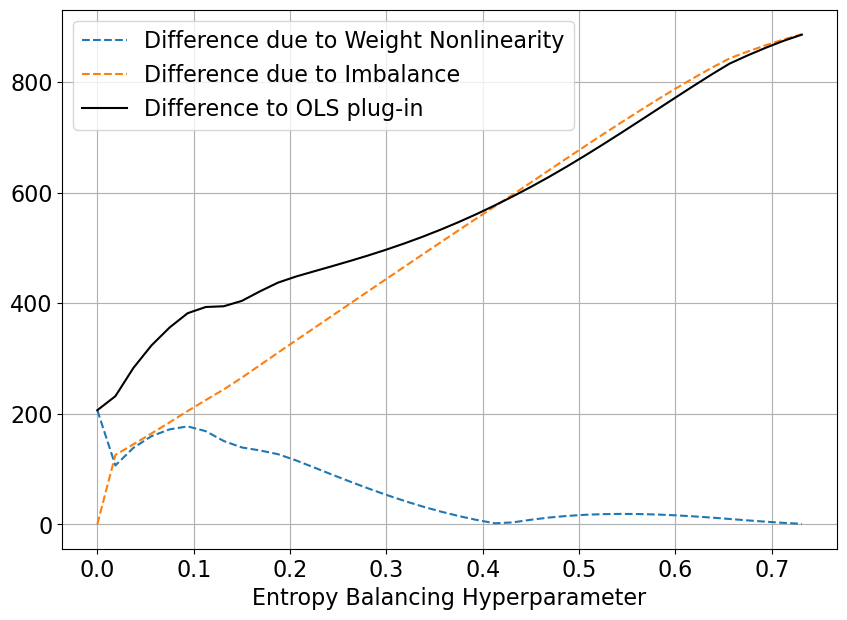
(a) Entropy Balancing

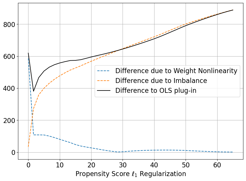
(b) Traditional IPW

Figure D.1: Decomposing the estimate from nonlinear augmented balancing weights for the “short” LaLonde (1986) example.

Figure D.1 shows that there are two countervailing features at play here. First, as the weights become linear, $\hat{\psi}\rightarrow\bar{\Phi}_{q}\hat{\beta}_{\text{aug}}$ with the difference quantified by Proposition D.1. This occurs as the regularization strength increases because regularization pushes the weights to be uniform. Second, as the imbalance goes to zero, $\hat{\beta}_{\text{aug}}\rightarrow\hat{\beta}_{\text{ols}}$. For entropy balancing, this happens exactly as the hyperparamater goes to zero. The IPW weights typically yield substantially larger imbalance, and this imbalance does not vanish as the regularization parameter goes to zero.

D.2 Constraining weights to be non-negative

A common modification of the (minimum variance) balancing weights problem is to constrain the estimated weights to be non-negative. Such weights have a number of attractive practical properties: they limit extrapolation; they ensure that the final weighting estimator is sample bounded; and they are typically sparse, which can sometimes aid interpretability (Robins et al., 2007; Abadie et al., 2010). Examples of constrained $\ell_{\infty}$ weights include Stable Balancing Weights and extensions (Zubizarreta, 2015; Athey et al., 2018; Wang and Zubizarreta, 2020); examples of constrained $\ell_{2}$ weights include popular variants of the synthetic control method (Abadie et al., 2010; Ben-Michael et al., 2021c).

Using the dual form of the problem, Ben-Michael et al. (2021b) show that (minimum variance) linear balancing weights with a non-negativity constraint have the form $\hat{w}=\{\Phi_{p}\hat{\theta}^{\delta}\}_{+}$, where $\{x\}_{+}=\text{max}(x,0)$ and where the coefficients $\hat{\theta}^{\delta}$ are generally different from the corresponding coefficients in the unconstrained model. We can apply this insight to extend Proposition 3.1 to non-negative weights.

Proposition D.2.

Let $\hat{w}^{\delta}_{+}\coloneqq\{\Phi_{p}\hat{\theta}^{\delta}\}_{+}$, with $\hat{\theta}^{\delta}\in\mathbb{R}^{d}$ and where $\{x\}_{+}=\text{max}(x,0)$, be any linear balancing weights with a non-negativity constraint, with corresponding weighted covariates $\hat{\Phi}_{q}^{\delta}\coloneqq\hat{w}_{+}\Phi_{p}$. Let $\Phi_{p+},$ and $Y_{p+}$ denote the respective quantities restricted to those data points where $\hat{w}^{\delta}_{+}>0$. Let $\hat{\beta}_{\text{ols}}^{+}\coloneqq(\Phi_{p+}^{\top}\Phi_{p+})^{-1}\Phi_{p+}^{\top}Y_{p+}$ be the OLS coefficients of the regression of $Y_{p+}$ on $\Phi_{p+}$. Then:

$$\hat{\mathbb{E}}\left[\hat{w}_{+}^{\delta}\circ Y_{p}\right]=\hat{\Phi}_{q}^{\delta}\hat{\beta}_{\text{ols}}^{+}.$$

So with the non-negativity constraint, we recover Proposition 3.1 almost exactly, except that the usual OLS coefficients from the entire population $p$, $\hat{\beta}_{\text{ols}}$, are replaced with the OLS coefficients from only those units with positive weight, $\hat{w}^{\delta}_{+}>0$, $\hat{\beta}_{\text{ols}}^{+}$. We can therefore view the non-negativity constraint as a form of sample trimming. In particular, we can think of the data points where $\hat{w}^{\delta}_{+}=0$ as a set of outliers — too dissimilar from the target population $\Phi_{q}$ — that we trim before applying OLS. But the key is that the definition of “outlier” depends the choice of $\delta$ and $\mathcal{F}$, and even the target covariates $\Phi_{q}$: in general, changing $\delta$, $\mathcal{F}$, or $\Phi_{q}$ will change the set where $\hat{w}^{\delta}_{+}>0$. Defining and characterizing how this set changes is a promising avenue for future research. Finally, note that it is not generally the case that re-estimating the balancing weights problem after sample trimming will lead to non-negative weights (though this does hold for OLS).

Proposition D.2 simplifies further when the balancing weights achieve exact balance; see Rubinstein et al. (2021, Proposition 10) for a discussion of this special case. When $\hat{\Phi}_{q}=\Phi_{q}$, the balancing weight estimator with the non-negativity constraint is equivalent to $\hat{\mathbb{E}}[\Phi_{q}\hat{\beta}_{\text{ols}}^{+}]$. Thus, linear balancing weights with a simplex constraint is equivalent to trimming the control group and applying standard OLS (note that the trimming does not affect the target covariate profile, $\Phi_{q}$).

Finally, we can extend the results in Proposition 3.2 for augmented balancing weights to incorporate a non-negativity constraint. Many popular augmented balancing weights estimators have the form of Proposition 3.2, including Athey et al. (2018) and Ben-Michael et al. (2021c). Understanding the implications of this connection is an interesting direction for future work.

D.3 Non-Linear Differentiable Outcome Models

In this section, we provide a very preliminary sketch of how the results might be extended to the case where $\mathcal{F}$ is non-linear but still differentiable in its parameters.

Let $\mathcal{F}=\{f(X,\theta):\theta\in\mathbb{R}^{d},\nabla_{\theta}f(X,\theta)\text{ exists}\}$. Then just like Proposition 3.1 relates any $w$ that are linear in $X$ to the OLS coefficients, we can relate any $w\in\mathcal{F}$ to the least squares regressor in the function class $\mathcal{F}$.

First, let $\theta_{\text{LS}}$ be the unregularized least squares regressor (where we choose the least norm $\theta$ to break ties):

$$\theta_{\text{LS}}\coloneqq\min_{\theta}\|Y_{p}-f(\theta,X_{p})\|_{2}^{2}$$

We have the first-order condition:

$$\nabla_{\theta}f(\theta_{\text{LS}},X_{p})^{\top}(Y_{p}-f(\theta_{\text{LS}},X_{p}))=0$$

Now we can get a version of Proposition 2.1 for $w\in\mathcal{F}$ by considering the following taylor expansion:

$$w(X_{p})\coloneqq f(\theta_{w},X_{p})\approx f(\theta_{\text{LS}},X_{p})+\nabla_{\theta}f(\theta_{\text{LS}},X_{p})(\theta_{w}-\theta_{\text{LS}})$$

In which case, applying the first-order condition above, we get:

$$w(X_{p})^{\top}y\approx\underbrace{w(X_{p})^{\top}f(\theta_{\text{LS}},X_{p})}_{\text{identical to 3.1}}+\underbrace{f(\theta_{\text{LS}},X_{p})^{\top}(Y_{p}-f(\theta_{\text{LS}},X_{p}))}_{\text{this term is zero in linear case}}.$$

Appendix E Results with Correlated Features

E.1 Overview

Throughout the main text, we have made the assumption that $\Phi_{p}^{\top}\Phi_{p}$ is a diagonal matrix. This is a useful simplifying assumption for illustrating the intuition behind our results. Our central result, Proposition 3.2, holds for arbitrary $\Phi_{p}^{\top}\Phi_{p}$. However, when $\Phi_{p}^{\top}\Phi_{p}$ is not diagonal, i.e. the covariates are correlated, there are some important additional subtleties for interpreting the results.

In Section E.2, we show that the results in the main text for $\ell_{2}$ balancing weights still hold for non-diagonal $\Phi_{p}^{\top}\Phi_{p}$ by applying an additional rotation step. By constrast, in Section E.3, we demonstrate that diagonal $\Phi_{p}^{\top}\Phi_{p}$ is not without loss of generality for $\ell_{\infty}$ balancing. Not only do the weights not have a closed form, but the resulting augmented coefficients will not be sparse.

E.2 Augmented $\ell_{2}$ Balancing Weights with Correlated Features

To begin, we provide the following characterization of $\ell_{2}$ augmenting with correlated features directly, that is, without using Proposition 3.2:

Proposition E.1.

Let $\hat{w}_{\ell_{2}}^{\delta}$ denote the solution to the penalized linear form of balancing weights with parameter $\delta$ and $\mathcal{F}=\{f(x)=\theta^{\top}\phi(x):\|\theta\|_{2}\leq r\}$. Then,

$$\hat{w}_{\ell_{2}}^{\delta}=\Phi_{p}(\Phi_{p}^{\top}\Phi_{p}+\delta I)^{-1}\mkern 1.5mu\overline{\mkern-1.5mu\Phi\mkern-1.5mu}\mkern 1.5mu_{q}.$$

Therefore, the augmented $\ell_{2}$ balancing weights estimator with outcome model $\hat{\beta}_{\text{reg}}\in\mathbb{R}^{d}$ has the form,

$$\hat{\mathbb{E}}[\Phi_{q}\hat{\beta}_{\text{reg}}]+\hat{\mathbb{E}}[\hat{w}_{\ell_{2}}^{\delta}(Y_{p}-\Phi_{p}\hat{\beta}_{\text{reg}})]=\hat{\mathbb{E}}[\Phi_{q}\hat{\beta}_{\ell_{2}}],$$

$$\hat{\beta}_{\ell_{2}}\coloneqq(I-A_{\delta})\hat{\beta}_{\text{reg}}+A_{\delta}\hat{\beta}_{\text{ols}}$$ (25)

$$A_{\delta}\coloneqq(\Phi_{p}^{\top}\Phi_{p}+\delta I)^{-1}(\Phi_{p}^{\top}\Phi_{p}).$$

For comparison, ridge regression with parameter $\delta$ has closed-form coefficients:

$$\hat{\beta}_{\text{ridge}}^{\delta}=(\Phi_{p}^{\top}\Phi_{p}+\delta I)^{-1}\Phi_{p}^{\top}Y_{p}=A_{\delta}\beta_{\text{ols}}.$$

This is a generalization of Proposition 4.1 to the correlated setting. The result follows by simply plugging in the closed-form of $\hat{w}^{\delta}_{\ell_{2}}$ into the augmented estimator. We will now show that the resulting $\hat{\beta}_{\ell_{2}}$ is equivalent to applying Proposition 3.2 to rotated versions of the outcome and weighting coefficients.

First, we define the rotated version of Proposition 3.2:

Proposition E.2.

Let $\Phi_{p}^{\top}\Phi_{p}$ be arbitrary, with eigendecomposition $\Phi_{p}^{\top}\Phi_{p}=VD^{2}V^{\top}$ where $D^{2}$ is a diagonal matrix with $j$th entry $\sigma_{j}^{2}$. For any $\hat{\beta}_{\text{reg}}^{\lambda}\in\mathbb{R}^{d}$, and any linear balancing weights estimator with estimated coefficients $\hat{\theta}^{\delta}\in\mathbb{R}^{d}$, and with $\hat{w}^{\delta}\coloneqq\hat{\theta}^{\delta}\Phi_{p}^{\top}$ and $\hat{\Phi}_{q}^{\delta}\coloneqq\hat{w}^{\delta}\Phi_{p}$, the resulting augmented estimator

$$\hat{\mathbb{E}}[\hat{w}^{\delta}\circ Y_{p}]+\hat{\mathbb{E}}\left[\left(\Phi_{q}-\hat{\Phi}_{q}^{\delta}\right)\hat{\beta}_{\text{reg}}^{\lambda}\right]$$

$$=\hat{\mathbb{E}}[\Phi_{q}V\hat{\beta}_{\text{aug}}^{\text{rot}}],$$

where the $j$th element of $\hat{\beta}_{\text{aug}}^{\text{rot}}$ is:

$$\hat{\beta}_{\text{aug},j}^{\text{rot}} \coloneqq\left(1-a_{j}^{\text{rot}}\right)\hat{\beta}_{\text{reg},j}^{\text{rot}}+a_{j}^{\text{rot}}\hat{\beta}_{\text{ols},j}^{\text{rot}}$$

$$a_{j}^{\text{rot}} \coloneqq\frac{\widehat{\Delta}_{j}^{\text{rot}}}{\Delta_{j}^{\text{rot}}},$$

defined in terms of the rotated quantities:

$$\hat{\beta}_{\text{reg}}^{\text{rot}} \coloneqq V^{\top}\hat{\beta}_{\text{reg}}^{\lambda},$$

$$\hat{\beta}_{\text{ols}}^{\text{rot}} \coloneqq V^{\top}\hat{\beta}_{\text{ols}},$$

$$\widehat{\Delta}^{\text{rot}} \coloneqq(\hat{\Phi}_{q}-\bar{\Phi}_{p})V,$$

$$\Delta^{\text{rot}} \coloneqq(\bar{\Phi}_{q}-\bar{\Phi}_{p})V.$$

Proof.

First notice that:

$$\hat{\mathbb{E}}[\hat{w}^{\delta}\circ Y_{p}]+\hat{\mathbb{E}}\left[\left(\Phi_{q}-\hat{\Phi}_{q}^{\delta}\right)\hat{\beta}_{\text{reg}}^{\lambda}\right]$$

$$=\hat{\mathbb{E}}\left[\hat{\Phi}_{q}^{\delta}\hat{\beta}_{\text{ols}}+\left(\Phi_{q}-\hat{\Phi}_{q}^{\delta}\right)\hat{\beta}_{\text{reg}}^{\lambda}\right]$$

$$=\hat{\mathbb{E}}\left[\hat{\Phi}_{q}^{\delta}VV^{\top}\hat{\beta}_{\text{ols}}+\left(\Phi_{q}-\hat{\Phi}_{q}^{\delta}\right)VV^{\top}\hat{\beta}_{\text{reg}}^{\lambda}\right]$$

Then the result follows immediately from Proposition 3.2 applied to the covariates $\Phi_{p}V$ and $\Phi_{q}V$ with weights $\hat{w}$ and outcome model $V^{\top}\hat{\beta}_{\text{reg}}^{\lambda}$. ∎

Note that we could also compute $\hat{\beta}_{\text{aug}}$ directly as in Proposition 3.2 because the original derivation does not depend on $\Phi_{p}^{\top}\Phi_{p}$ being diagonal. Combining the two propositions we have that:

$$\hat{\mathbb{E}}[\Phi_{q}\hat{\beta}_{\text{aug}}]=\hat{\mathbb{E}}[\Phi_{q}V\hat{\beta}_{\text{aug}}^{\text{rot}}].$$

However, it is not the case that $\hat{\beta}_{\text{aug}}=V\hat{\beta}_{\text{aug}}^{\text{rot}}$ in general. For $\ell_{2}$ balancing weights, $V\hat{\beta}^{\text{rot}}_{\text{aug}}$ is the correct generalization of Proposition 3.2 to the correlated setting as we demonstrate in the next few propositions.

Proposition E.3.

Let $\hat{\beta}_{\ell_{2}}$ be defined as in Equation 25. For the same weights $\hat{w}_{\ell_{2}}^{\delta}$, let $\hat{\beta}_{\text{aug}}$ and $\hat{\beta}_{\text{aug}}^{\text{rot}}$ be defined as in Propositions 3.2 and E.2 respectively. Then for any $\Phi_{p}^{\top}\Phi_{p}$ (diagonal or not):

$$\hat{\mathbb{E}}[\Phi_{q}\hat{\beta}_{\ell_{2}}]=\hat{\mathbb{E}}[\Phi_{q}V\hat{\beta}_{\text{aug}}^{\text{rot}}]=\hat{\mathbb{E}}[\Phi_{q}\hat{\beta}_{\text{aug}}].$$

Additionally, when $\Phi_{p}^{\top}\Phi_{p}$ is diagonal, then

$$\hat{\beta}_{\ell_{2}}=V\hat{\beta}_{\text{aug}}^{\text{rot}}=\hat{\beta}_{\text{aug}}.$$

However, when $\Phi_{p}^{\top}\Phi_{p}$ is not diagonal, then in general

$$\hat{\beta}_{\ell_{2}}=V\hat{\beta}_{\text{aug}}^{\text{rot}}\neq\hat{\beta}_{\text{aug}}.$$

Proof.

The fist claims follows from Propositions 3.2, E.2, and E.1. For the second claim, if $\Phi_{p}^{\top}\Phi_{p}$ is diagonal, then $V=I$ and $\hat{\beta}_{\text{aug}}=\hat{\beta}_{\text{aug}}^{\text{rot}}$. Next we will show for general $\Phi_{p}^{\top}\Phi_{p}$ that $\hat{\beta}_{\ell_{2}}=V\hat{\beta}_{\text{aug}}^{\text{rot}}$. Note that

$$A_{\delta}=V(D^{2}+\delta I)^{-1}D^{2}V^{\top},$$

and that

$$\hat{\Delta}^{\text{rot}} =\mkern 1.5mu\overline{\mkern-1.5mu\Phi\mkern-1.5mu}\mkern 1.5mu_{q}(\Phi_{p}^{\top}\Phi_{p}+\delta I)^{-1}(\Phi_{p}^{\top}\Phi_{p})V$$

$$=\mkern 1.5mu\overline{\mkern-1.5mu\Phi\mkern-1.5mu}\mkern 1.5mu_{q}V(D^{2}+\delta I)^{-1}D^{2}$$

and so $\text{diag}(a^{\text{rot}})=(D^{2}+\delta I)^{-1}D^{2}$. Therefore,

$$V\hat{\beta}_{\text{aug}}^{\text{rot}} =V(I-\text{diag}(a^{\text{rot}}))V^{\top}\hat{\beta}_{\text{reg}}+V\text{diag}(a^{\text{rot}})V^{\top}\hat{\beta}_{\text{ols}}$$

$$=(VV^{\top}-A_{\delta})\hat{\beta}_{\text{reg}}+A_{\delta}\hat{\beta}_{\text{ols}}$$

$$=(I-A_{\delta})\hat{\beta}_{\text{reg}}+A_{\delta}\hat{\beta}_{\text{ols}}.$$

Finally, for a counter-example where $V\hat{\beta}^{\text{rot}}_{\text{aug}}\neq\hat{\beta}_{\text{aug}}$, see Section E.2. ∎

Proposition E.4.

Consider the setting in Proposition E.3, but now assume that the outcome model $\hat{\beta}_{\text{reg}}=\hat{\beta}_{\text{ridge}}^{\lambda}$, the ridge regression coefficients of $Y_{p}$ on $\Phi_{p}$ with hyperparameter $\lambda$. Then:

$$\hat{\beta}_{\ell_{2}}=V(D^{2}+\text{diag}(\gamma))^{-1}V^{\top}\Phi_{p}^{\top}Y_{p},$$

where $\text{diag}(\gamma)$ is the diagonal matrix with $j$th entry

$$\gamma_{j}\coloneqq\frac{\delta\lambda}{\sigma_{j}^{2}+\lambda+\delta}.$$

Furthermore,

$$\|\hat{\beta}_{\text{ridge}}^{\lambda}\|_{2}\leq\|\hat{\beta}_{\ell_{2}}\|_{2}=\|V\hat{\beta}_{\text{aug}}^{\text{rot}}\|_{2}\leq\|\hat{\beta}_{\text{ols}}\|_{2},$$

but in general it is possible that:

$$\|\hat{\beta}_{\text{ols}}\|_{2}<\|\hat{\beta}_{\text{aug}}\|_{2}.$$

Proof.

$$\hat{\beta}_{\ell_{2}} =(I-A_{\delta})(\Phi_{p}^{\top}\Phi_{P}+\lambda I)^{-1}\Phi_{p}^{\top}Y_{p}+A_{\delta}(\Phi_{p}^{\top}\Phi_{P})^{-1}\Phi_{p}^{\top}Y_{p}$$

$$=V\Big{[}(I-(D^{2}+\delta I)^{-1}D^{2})(D^{2}+\lambda I)^{-1}+(D^{2}+\delta I)^{-1}D^{2}(D^{2})^{-1}\Big{]}V^{\top}\Phi_{p}^{\top}Y_{p}$$

$$=V(D^{2}+(\delta+\lambda)I)(D^{2}+\delta I)^{-1}(D^{2}+\lambda I)^{-1}V^{\top}\Phi_{p}^{\top}Y_{p}$$

$$=V(D^{2}+\text{diag}(\gamma))^{-1}V^{\top}\Phi_{p}^{\top}Y_{p}.$$

We now demonstrate the two norm inequalities. First,

$$\|\hat{\beta}_{\text{ridge}}^{\lambda}\|_{2}^{2}\leq\|\hat{\beta}_{\ell_{2}}\|_{2}^{2}$$

$$\iff \|V(D^{2}+\lambda I)^{-1}V^{\top}\Phi_{p}^{\top}Y_{p}\|_{2}^{2}\leq\|V(D^{2}+\textnormal{diag}(\gamma))^{-1}V^{\top}\Phi_{p}^{\top}Y_{p}\|_{2}^{2}$$

$$\iff Y_{p}^{\top}\Phi_{p}(V\left[(D^{2}+\lambda I)^{-1}(D^{2}+\lambda I)^{-1}-(D^{2}+\textnormal{diag}(\gamma))^{-1}(D^{2}+\textnormal{diag}(\gamma))^{-1}\right]V^{\top})\Phi_{p}^{\top}Y_{p}\geq 0$$

$$\iff (D^{2}+\lambda I)^{-1}(D^{2}+\lambda I)^{-1}\preceq(D^{2}+\textnormal{diag}(\gamma))^{-1}(D^{2}+\textnormal{diag}(\gamma))^{-1}$$

$$\iff (D^{2}+\lambda I)^{-1}\preceq(D^{2}+\textnormal{diag}(\gamma))^{-1}.$$

Note that

$$\frac{1}{\sigma^{2}_{j}+\gamma_{j}}=\left(\frac{1}{\sigma_{j}^{2}+\lambda}\right)\left(\frac{\sigma_{j}^{2}+\lambda+\delta}{\sigma_{j}^{2}+\delta}\right),$$ (26)

and that

$$\frac{\sigma_{j}^{2}+\lambda+\delta}{\sigma_{j}^{2}+\delta}\geq 1.$$ (27)

Combining facts (26) and (27), we have $1/(\sigma^{2}_{j}+\gamma_{j})>1/(\sigma^{2}_{j}+\lambda)$, and we’re done.

Similarly, for the second inequality:

$$\|\hat{\beta}_{\ell_{2}}\|_{2}^{2}\leq\|\hat{\beta}_{\text{ols}}\|_{2}^{2}$$

$$\iff \|V(D^{2}+\text{diag}(\gamma))^{-1}V^{\top}\Phi_{p}^{\top}Y_{p}\|_{2}^{2}\leq\|V(D^{2})^{-1}V^{\top}\Phi_{p}^{\top}Y_{p}\|_{2}^{2}$$

$$\iff (D^{2}+\textnormal{diag}(\gamma))^{-1}\preceq(D^{2})^{-1}$$

which follows because $\gamma\geq 0$.

Finally, for a counter-example where $\|\hat{\beta}_{\text{ols}}\|_{2}<\|\hat{\beta}_{\text{aug}}\|_{2}$, see Table E.1. ∎

Even when $\Phi_{p}^{\top}\Phi_{p}$ is diagonal, if $\hat{\beta}_{\text{reg}}$ can be arbitrary — and in particular, adversarially chosen — then we are not guaranteed to see undersmoothing. Consider an arbitrary $\hat{\beta}_{\text{reg}}$ that $\ell_{2}$-smoothed with respect to OLS. That is, $\|\hat{\beta}_{\text{reg}}\|_{2}\leq\|\hat{\beta}_{\text{ols}}\|_{2}$. If there are no other constraints on $\hat{\beta}_{\text{reg}}$, then there exist problem instances where $\hat{\beta}_{\ell_{2}}$ has $\ell_{2}$-norm larger than $\hat{\beta}_{\text{ols}}$ or smaller than $\hat{\beta}_{\text{reg}}$. For a simple example, consider $a^{\delta}=[0,1/(1+\delta)]$, and $\hat{\beta}_{\text{ols}}=[0,1]$ — note that these are jointly realizable by some $\Phi_{p},Y_{p}$. Then $\hat{\beta}_{\text{reg}}=[1,0]$ will have $\ell_{2}$-norm bigger than $1$ for sufficiently large $\delta$.

Empirical Results for augmented $\ell_{2}$-balancing weights.

To see in practice that the rotated procedure obtains the properly undersmoothed augmented coefficients, we report norm values for $\ell_{2}$ augmented estimators using both a ridge and a lasso base learner in the high-dimensional LaLonde and IHDP settings. The key takeaway is that $\hat{\beta}_{\ell_{2}}=V\hat{\beta}^{\text{rot}}_{\text{aug}}$ has the correct undersmoothing properties.

$\hat{\beta}_{\text{reg}}$	$\|\hat{\beta}_{\text{reg}}\|_{2}$	$\|\hat{\beta}_{\ell_{2}}\|_{2}$	$\|\hat{\beta}_{\text{ols}}\|_{2}$	$\|\hat{\beta}_{\text{aug}}\|_{2}$
LaLonde Ridge	6.495e3	1.160e4	4.469e7	4.633e7
LaLonde Lasso	7.273e3	1.154e4	4.469e7	4.633e7
IHDP Ridge	1.038	8.569	9.299	9.722
IHDP Lasso	1.262	8.666	9.299	9.626

Table E.1: The $\ell_{2}$ norm of base learner coefficients, unrotated augmented coefficients, OLS coefficients, and properly rotated augmented coefficients. Results are reported for the LaLonde and IHDP datasets using their respective high-dimensional feature sets and with both ridge and lasso base learners.

E.3 Augmented $\ell_{\infty}$ balancing weights

When we use $\ell_{\infty}$ balancing for the weighting model (or equivalently the minimum distance lasso estimator for the Riesz representer), the story becomes more complicated. When $\Phi_{p}^{\top}\Phi_{p}$ is not diagonal, both the Lasso outcome model and the $\ell_{\infty}$ balancing weights lack a closed-form solution.

For Lasso with correlated features, the regularization path is qualitatively similar to the diagonal case. The coefficients start at OLS and shrink exactly to zero at different rates. However, due to the correlation between the features, each coefficient no longer linearly (or even monotonically) moves toward zero. Likewise, for $\ell_{\infty}$ balancing weights, we see similar behavior for the coefficients of the Riesz representer model. These coefficients are sparse, with regularization paths that move toward zero (but not monotonically).

In the diagonal setting, the regularization path for the augmented estimator, $a_{j}^{\delta}$, is proportionate (element-wise) to $\hat{\theta}$. Therefore, because $\hat{\theta}$ is sparse, the augmented estimator coefficients defined in Proposition 3.2 is also sparse. For general design, the impact of $\hat{\theta}$ on the augmented coefficients also depends on the empirical covariance matrix.

Lemma E.5.

Let $\hat{w}$ be the solution to balancing weights with hyperparameter $\delta$ for $\mathcal{F}=\{f(x)=\theta^{\top}\phi(x):\|\theta\|\leq r\}$, where $\|\cdot\|$ is any norm. Let $\hat{\theta}$ be the corresponding solution to the dual form of balancing weights, so that $\hat{w}=\Phi_{p}\hat{\theta}$. Then,

$$\hat{\Phi}_{q}=\hat{\theta}^{\top}\Sigma,$$

and

$$a_{j}^{\delta}=\frac{\hat{\theta}^{\top}\Sigma_{j}}{\mkern 1.5mu\overline{\mkern-1.5mu\Phi\mkern-1.5mu}\mkern 1.5mu_{q,j}}.$$

In the case of $\ell_{\infty}$ balancing, since $\hat{\theta}$ is sparse, $a_{j}^{\delta}$ is a sparse combination of the elements of the $j$th column of the empirical covariance matrix $\Sigma$. But unless this combination is exactly zero (typically a measure zero event), the resulting $a^{\delta}$ will not inherit sparsity from $\hat{\theta}$.

Appendix F Additional Numerical Experiments

F.1 Dataset Summaries

The following table summarizes the number of samples and features in the datasets used for numerical illustrations. In the main text, we presented results for “LaLonde Short” and “LaLonde Long”, the LaLonde (1986) data with the original 11 features and the expanded 171 features from Farrell (2015).

In Section F.3, we also provide results for the Infant Health and Development Program (IHDP) dataset, a standard observational causal inference benchmark from Hill (2011). IHDP is based on data from a randomized control trial of an intensive home visiting and childcare intervention for low birth weight infants born in 1985. For all children, we have a range of baseline covariates (contained in “IHDP Short”), including both categorical covariates, like the mother’s educational attainment, and continuous covariates, like the child’s birth weight. Our goal is to estimate the average outcome (a standardized test score) in the absence of the intensive intervention. We additionally create an “IHDP Long” extended feature set that includes all pair-wise interaction terms between the discrete covariates and a second-order polynomial expansion of all continuous covariates.

Dataset	Features	Train Samples	Test Samples
LaLonde Short	11	727	185
LaLonde Long	171	727	185
IHDP Short	25	608	139
IHDP Long	193	608	139

Table F.2: Summary of the four datasets used for numerical illustrations including the number of features, the number of control/train observations (used as samples from $p$) and the number of treated/test observations (used as samples from $q$).

F.2 Numerical Example with cross-fitting

In Section 6.1, we demonstrated that for the low-dimensional NSW setting, the cross-validated weighting hyperparameter is $\delta=0$. As a result, for any linear base learner, the augmented estimator is numerically equivalent to a simple OLS plug-in estimate. As discussed in Section C.3, with cross-fitting this should only remain approximately true. In this section, we numerically assess the sensitivity of this result to cross-fitting.

We repeat the experiment with the 11-dimensional NSW covariates using a lasso base learner and $\ell_{\infty}$ balancing weights. We perform 5-fold cross-fitting with random splits. In each split, we compute the augmented estimate using models fit with data from the other 4 splits as described at the beginning of Appendix C. Each model has its hyperparameter chosen separately by cross-validation. Thus for 5-fold cross-fitting, we fit 5 lasso regressions and 5 balancing weights estimators each with $4/5$ths the sample size and a separate hyperparameter. In the manner of bootstrapping, we re-run this end-to-end procedure 1000 times for different random choices of the splits.

Note that there are two main ways that cross-fitting might cause the final estimate to deviate from simple OLS. The first is the variation due to only applying the models out of sample. The second is that with smaller sample sizes, cross-validation might select larger values for the hyperparameter. We find that for 80% of the $5\times 1000$ weighting models, $\delta=0$. In the remaining 20% some of the hyperparameters take on a very small but non-zero value. The mean $\delta$ is 0.0037 and the CDF across the $5\times 1000$ models is given in Figure 2(a).

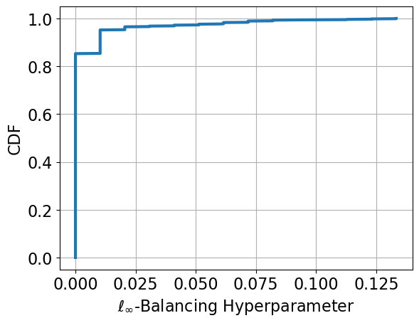
(a) Weighting Hyperparameter CDF

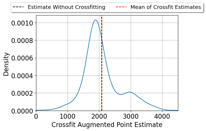
(b) Distribution of cross-fit Estimates

Figure F.2: Results with 5-fold cross-fitting for the LaLonde (1986) dataset with the low-dimensional set of 11 features. The cross-fitting procedure is repeated $1000$ times. Panel (a) plots the empirical cumulative distribution of weighting hyperparameters over the $1000\times 5$ weighting models; in the main text, the $\ell_{\infty}$ hyperparameter extends from 0 to 1 (here truncated at 0.12). Panel (b) shows a density plot for the cross-fit augmented point estimates over the $1000$ repeats.

Figure 2(b) shows a smoothed density plot for the cross-fit augmented estimates over the 1000 draws. The black dotted line marks the augmented estimate without cross-fitting (recall that this is identical to the plug-in OLS estimate for this dataset). The red dotted line marks the mean of the cross-fit estimates over the 1000 draws. On average, cross-fitting has virtually no effect on the augmented estimate — at least in this setting where the weighting hyperparameter is usually close to zero. However, there is substantial variation across the 1000 draws. In particular, the density is skewed and the mode of the cross-fit estimates is slightly smaller than the OLS point estimate. There is also a meaningful tail of estimates larger than the OLS point estimate, including a second larger mode.

F.3 Additional Experiments

F.3.1 Low Dimensional

We begin by providing corroborating results for the low dimensional setting. We repeat the experiments in Section 6.1 in three additional settings: the LaLonde low-dimensional setting with $\ell_{2}$ balancing weights in Figure F.3, the IHDP low-dimensional setting with $\ell_{\infty}$ balancing weights in Figure F.4, and the IHDP low-dimensional setting with $\ell_{2}$ balancing weights in Figure F.5. In all of these cases, cross-validation for the weighting hyperparameter choose $\delta=0$, and thus the augmented estimator is equivalent to the OLS plug-in estimate. These plots can be compared to Figure 3 in the main text.

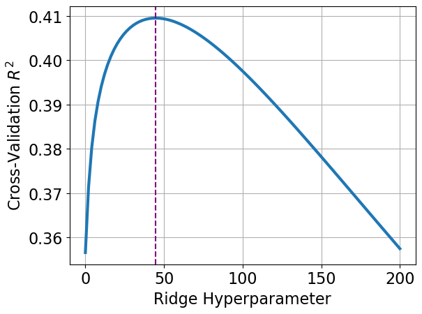
(a) Ridge outcome model

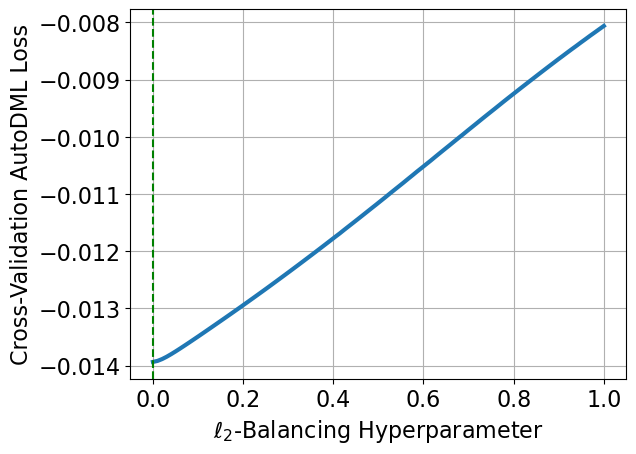
(b) $\ell_{2}$ balancing

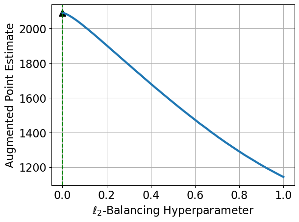
(c) Augmented estimate

Figure F.3: Ridge-augmented $\ell_{2}$ balancing weights (“double ridge”) for LaLonde (1986) with the original 11 features. Panel (a) shows the 10-fold cross-validated $R^{2}$ for the Ridge-penalized regression of $Y_{p}$ on $\Phi_{p}$ among control units across the hyperparameter $\lambda$; the purple dotted line shows the CV-optimal value. Panel (b) shows the 10-fold cross-validated AutoDML loss (8) for $\ell_{2}$ balancing weights across the hyperparameter $\delta$; the green dotted line shows the CV-optimal value, which is $\delta=0$ or exact balance. Panel (c) shows the point estimate for the augmented estimator across the weighting hyperparameter $\delta$; the black triangle corresponds to the OLS point estimate, which is also the CV-optimal value based on cross-validating the AutoDML loss.

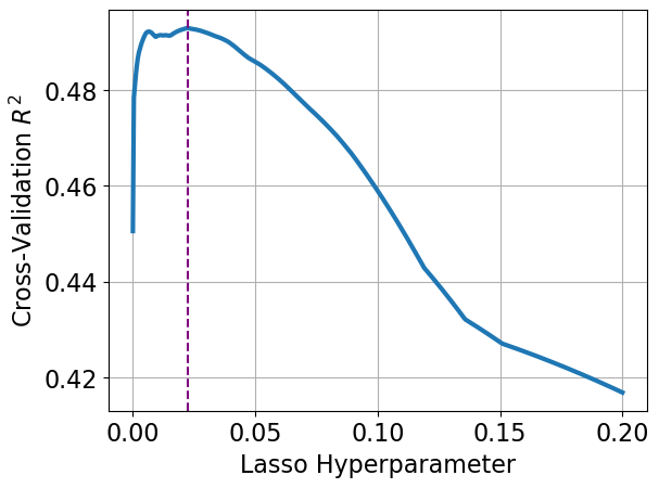
(a) Lasso outcome model

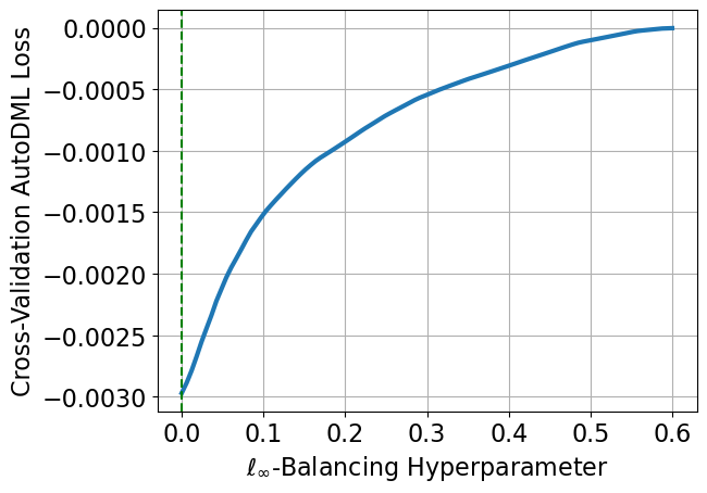
(b) $\ell_{\infty}$ balancing

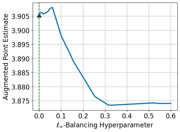
(c) Augmented estimate

Figure F.4: Lasso-augmented $\ell_{\infty}$ balancing weights (“double lasso”) for IHDP with the original 25 covariates. Panel (a) shows the 10-fold cross-validated $R^{2}$ for the Lasso-penalized regression of $Y_{p}$ on $\Phi_{p}$ among control units across the hyperparameter $\lambda$; the purple dotted line shows the CV-optimal value. Panel (b) shows the 10-fold cross-validated AutoDML loss (8) for $\ell_{\infty}$ balancing weights across the hyperparameter $\delta$; the green dotted line shows the CV-optimal value, which is $\delta=0$ or exact balance. Panel (c) shows the point estimate for the augmented estimator across the weighting hyperparameter $\delta$; the black triangle corresponds to the OLS point estimate, which is also the CV-optimal value based on cross-validating the AutoDML loss.

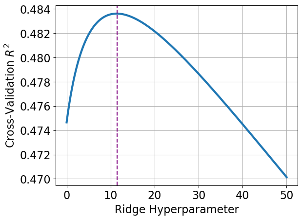
(a) Ridge outcome model

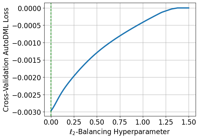
(b) $\ell_{2}$ balancing

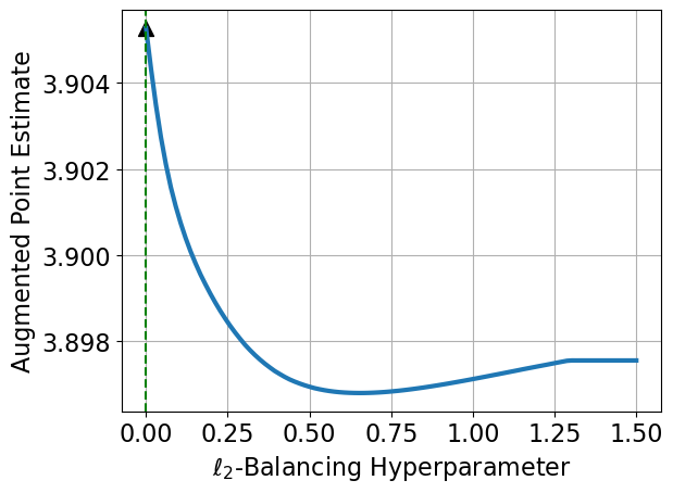
(c) Augmented estimate

Figure F.5: Ridge-augmented $\ell_{2}$ balancing weights (“double ridge”) for IDHP with the original 25 covariates. Panel (a) shows the 10-fold cross-validated $R^{2}$ for the Ridge-penalized regression of $Y_{p}$ on $\Phi_{p}$ among control units across the hyperparameter $\lambda$; the purple dotted line shows the CV-optimal value. Panel (b) shows the 10-fold cross-validated AutoDML loss (8) for $\ell_{2}$ balancing weights across the hyperparameter $\delta$; the green dotted line shows the CV-optimal value, which is $\delta=0$ or exact balance. Panel (c) shows the point estimate for the augmented estimator across the weighting hyperparameter $\delta$; the black triangle corresponds to the OLS point estimate, which is also the CV-optimal value based on cross-validating the AutoDML loss.

F.3.2 High Dimensional

We also replicate the experiments in Section 6.2 for high dimensional double ridge and double lasso but using the IHDP data with a high dimensional feature set. Figure F.6 replicates the reporting of point estimates and cross-validation curves for double lasso and double ridge with IHDP as in Figure 4; Figure F.7 replicates undersmoothing in double ridge as in Figure 5; and Figure F.8 replicates undersmoothing in the $\ell_{0}$ “norm” as in Figure 6.

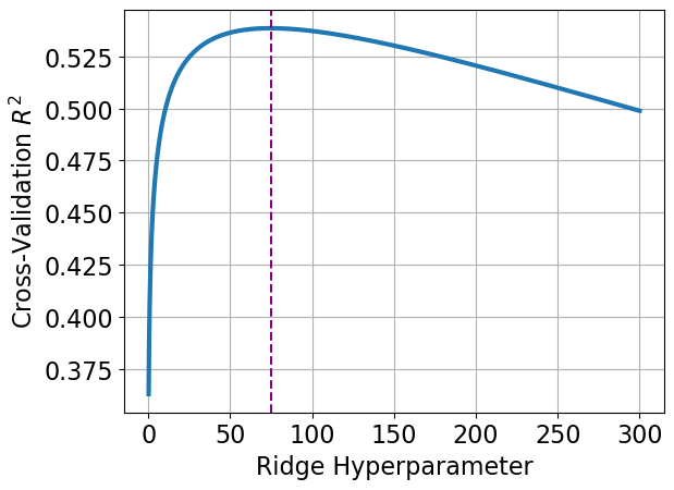
(a) Ridge outcome model

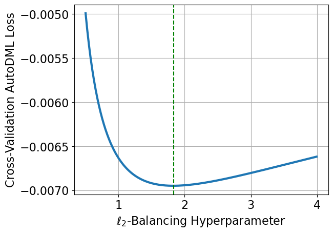
(b) $\ell_{2}$ balancing

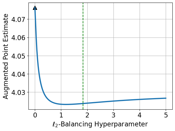
(c) Estimate from “double ridge”

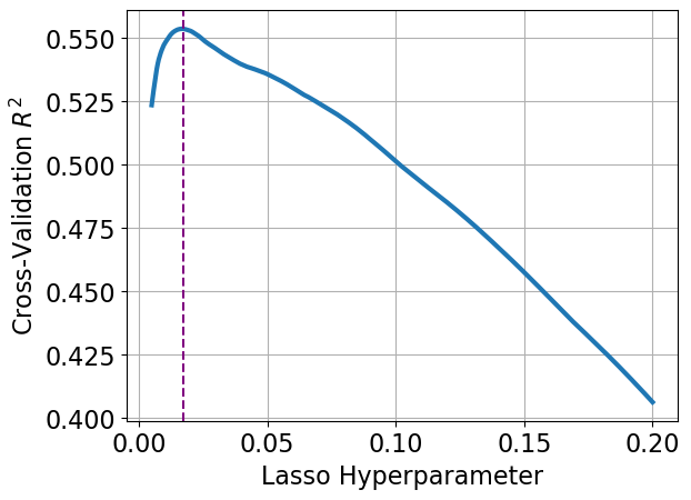
(d) Lasso outcome model

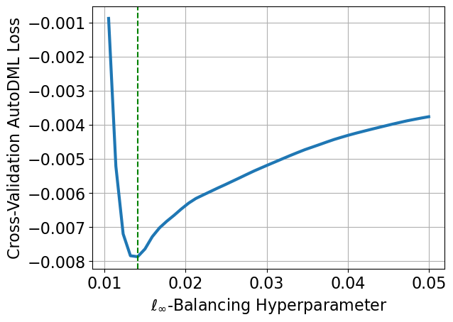
(e) $\ell_{\infty}$ balancing

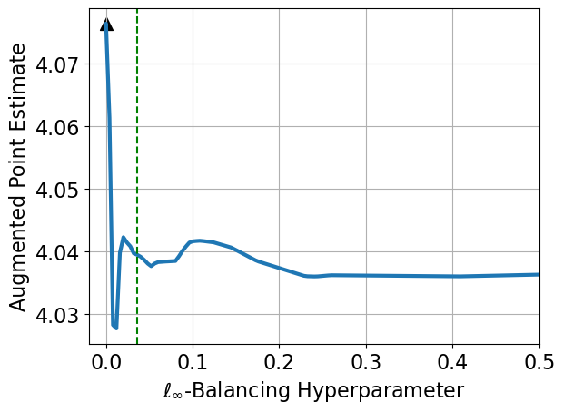
(f) Estimate from “double lasso”

Figure F.6: Augmented balancing weights estimates for the IHDP data set with the expanded set of 193 features; the top row shows ridge-augmented $\ell_{2}$ balancing, and the bottom row shows lasso-augmented $\ell_{\infty}$ balancing. Panels (a) and (d) show the 3-fold cross-validated $R^{2}$ for the ridge- and laso-penalized regression of $Y_{p}$ on $\Phi_{p}$ among control units across the hyperparameter $\lambda$; the purple dotted lines show the CV-optimal value for each. Panel (b) and (e) show the 10-fold cross-validated AutoDML loss (8) for $\ell_{2}$ and $\ell_{\infty}$ balancing weights across the hyperparameter $\delta$; the green dotted lines show the CV-optimal value for each. Panels (c) and (f) show the point estimates for the augmented estimators across the weighting hyperparameter $\delta$; the black triangles correspond to the OLS point estimate, and the green dotted lines show the CV-optimal value of $\delta$ for each.

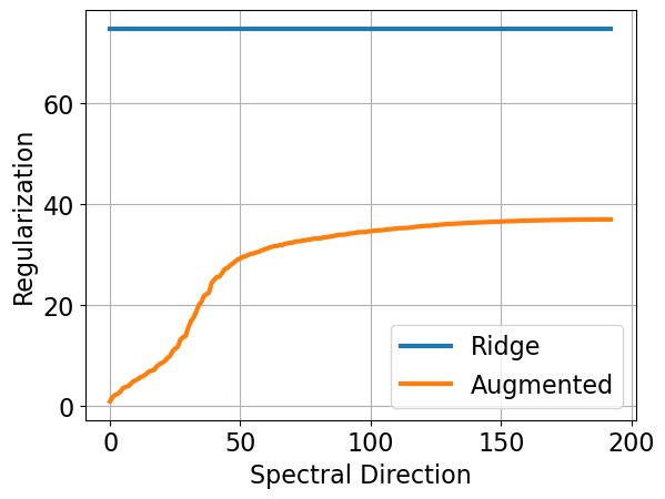
(a) Adaptive regularization

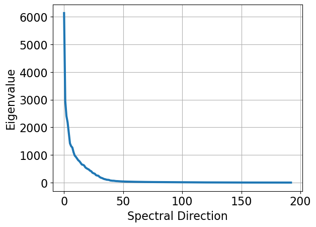
(b) Eigenvalues of $\Phi_{p}^{\top}\Phi_{p}$

Figure F.7: Single and double ridge regression applied to the “high-dimensional” version of the IHDP data set. Panel (a) shows $\lambda_{j}$, the single ridge hyperparameter, and $\gamma_{j}$, the implied double ridge hyperparameter, as functions of the spectral direction $j$. Panel (b) shows the corresponding eigenvalues.

(a) $\ell_{0}$ “norm” for ridge outcome model

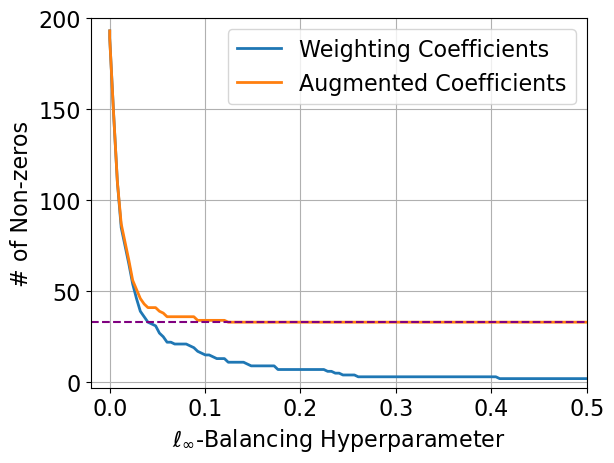
(b) $\ell_{0}$ “norm” for weighting and double lasso

Figure F.8: Undersmoothing in $\ell_{0}$ “norm” for augmented balancing weights applied to the “high dimesional” version of the IHDP data set. Panels (a) shows the number of non-zero covariates (the $\ell_{0}$ “norm”) for lasso regression of $Y_{p}$ on $\Phi_{p}$ among control units. Panels (b) shows the number of non-zero covariates for the weighting model and augmented coefficients. The dotted purple line is the outcome model hyperparameter chosen via cross validation.

Appendix G Additional Proofs

Closed forms for $\ell_{2}$ and exact balancing weights..

We derive the closed form for $\ell_{2}$ balancing weights with parameter $\delta$ (with exact balance following as a special case). The optimization problem:

$$\min_{w\in\mathbb{R}^{n}}\|w^{\top}\Phi_{p}-\bar{\Phi}_{q}\|_{2}^{2}+\delta\|w\|_{2}^{2}=w^{\top}\Phi_{p}\Phi_{p}^{\top}w-2w^{\top}\Phi_{p}\bar{\Phi}_{q}+\delta w^{\top}w$$

has first order condition:

$$2(\Phi_{p}\Phi_{p}^{\top}+\delta I_{n})w-2\Phi_{p}\bar{\Phi}_{q}=0,$$

which gives the solution:

$$w^{*} =(\Phi_{p}\Phi_{p}^{\top}+\delta I_{n})^{\dagger}\Phi_{p}\bar{\Phi}_{q}$$

$$=\Phi_{p}(\Phi_{p}^{\top}\Phi_{p}+\delta I_{d})^{\dagger}\bar{\Phi}_{q}.$$

∎

Proof of Proposition 4.1.

We apply Proposition 3.2. We have $a_{j}^{\delta}=\hat{\Phi}_{q,j}^{\delta}/\bar{\Phi}_{q,j}^{\delta}$. Then:

$$\hat{\Phi}_{q}^{\delta} =\hat{w}_{\ell_{2}}^{\delta}\Phi_{p}=\mkern 1.5mu\overline{\mkern-1.5mu\Phi\mkern-1.5mu}\mkern 1.5mu_{q}(\Phi_{p}^{\top}\Phi_{p}+\delta I)^{-1}\Phi_{p}^{\top}\Phi_{p}.$$

Since we have assumed that $\Phi_{p}^{\top}\Phi_{p}$ is diagonal, with $j$th diagonal entry, $\sigma_{j}^{2}$, we have:

$$\hat{\Phi}_{q,j}^{\delta}=\left(\frac{\sigma_{j}^{2}}{\sigma_{j}^{2}+\delta}\right)\bar{\Phi}_{q,j}.$$

Plugging this back into $a_{j}^{\delta}$ completes the proof. ∎

Proof of Proposition 4.3.

Applying Proposition Proposition 4.1:

$$\hat{\beta}_{\text{$\ell_{2}$},j} =\left(\frac{\sigma^{2}_{j}}{\sigma^{2}_{j}+\delta}\right)\hat{\beta}_{\text{ols,j}}+\left(\frac{\delta}{\sigma^{2}_{j}+\delta}\right)\hat{\beta}_{\text{ridge,j}}^{\lambda}$$

$$=\left(\frac{\sigma^{2}_{j}}{\sigma^{2}_{j}+\delta}\right)\hat{\beta}_{\text{ols,j}}+\left(\frac{\delta}{\sigma^{2}_{j}+\delta}\right)\left(\frac{\sigma^{2}_{j}}{\sigma^{2}_{j}+\lambda}\right)\hat{\beta}_{\text{ols},j}$$

$$=\frac{\sigma^{2}_{j}(\sigma_{j}^{2}+\lambda+\delta)}{(\sigma^{2}_{j}+\delta)(\sigma^{2}_{j}+\lambda)}\hat{\beta}_{\text{ols,j}}$$

Then taking:

$$\frac{\sigma^{2}_{j}(\sigma_{j}^{2}+\lambda+\delta)}{(\sigma^{2}_{j}+\delta)(\sigma^{2}_{j}+\lambda)}=\frac{\sigma_{j}^{2}}{\sigma_{j}^{2}+\gamma_{j}}$$

and solving for $\gamma_{j}$ gives:

$$\gamma_{j}\coloneqq\frac{\delta\lambda}{\sigma_{j}^{2}+\lambda+\delta}$$

which completes the proof. ∎

Proof of Proposition 5.1.

We begin with the constrained form of the balancing problem:

$$\min_{w\in\mathbb{R}^{n}} \|w\|_{2}^{2}$$

such that $$\left\|w\Phi_{p}-\bar{\Phi}_{q}\right\|_{\infty}\leq\delta.$$

Note that we can rewrite the norm constraint as two vector-valued linear constraints:

$$w\Phi_{p} \preceq\bar{\Phi}_{q}+\delta$$

$$-w\Phi_{p} \preceq-\bar{\Phi}_{q}+\delta,$$

which results in the Lagrangian,

$$\mathcal{L}(w,\mu,\nu)=\|w\|_{2}^{2}+\mu^{\top}\left(w\Phi_{p}-\bar{\Phi}_{q}-\delta\right)-\nu^{\top}\left(w\Phi_{p}-\bar{\Phi}_{q}+\delta\right).$$

The first-order conditions for the optimal $w^{*},\mu^{*},\nu^{*}$ are:

$$w^{*}=-\frac{1}{2}\left(\Phi_{p}\mu^{*}-\Phi_{p}\nu^{*}\right)$$

$$\mu_{j}^{*}\left(w^{*}\Phi_{p,j}-\bar{\Phi}_{q,j}-\delta\right)=0,\forall j$$

$$\nu_{j}^{*}\left(w^{*}\Phi_{p,j}-\bar{\Phi}_{q,j}+\delta\right)=0,\forall j$$

$$\mu_{j}^{*},\nu_{j}^{*}\geq 0,\forall j$$

plus the linear constraints on $w^{*}\Phi_{p}$. Note that the linear constraints plus the complimentary slackness conditions imply that one of three mutually-exclusive cases holds for each covariate. Case 1: $w^{*}\Phi_{p,j}=\bar{\Phi}_{q,j}-\delta$, in which case $\mu^{*}_{j}=0$. Case 2: $w^{*}\Phi_{p,j}=\bar{\Phi}_{q,j}+\delta$, in which case $\nu^{*}_{j}=0$. Or Case 3: $w^{*}\Phi_{p,j}\in(\bar{\Phi}_{q,j}-\delta,\bar{\Phi}_{q,j}+\delta)$, in which case $\mu^{*}_{j}=\nu^{*}_{j}=0$.

Define:

$$\theta^{*}_{j}\coloneqq\begin{cases}0&\text{if }w^{*}\Phi_{p,j}\in(\bar{\Phi}_{q,j}-\delta,\bar{\Phi}_{q,j}+\delta)\\ -\mu_{j}^{*}/2&\text{if }w^{*}\Phi_{p,j}=\bar{\Phi}_{q,j}+\delta\\ \nu_{j}^{*}/2&\text{if }w^{*}\Phi_{p,j}=\bar{\Phi}_{q,j}-\delta.\end{cases}$$

Then we have $w^{*}=\Phi_{p}\theta^{*}$ from the first-order condition, and thus $w^{*}\Phi_{p}=(\Phi_{p}^{\top}\Phi_{p})\theta^{*}$. Using the fact that $(\Phi_{p}^{\top}\Phi_{p})$ is diagonal, we get $w^{*}\Phi_{p,j}=\sigma_{j}^{2}\theta^{*}_{j}$.

Finally, we can plug this into the three cases that define $\theta^{*}$. First, $\theta_{j}^{*}=0$ when

$$\sigma^{2}_{j}\theta_{j}^{*}\in(\bar{\Phi}_{q}-\delta,\bar{\Phi}_{q}+\delta)$$

$$\implies 0\in(\bar{\Phi}_{q}-\delta,\bar{\Phi}_{q}+\delta)$$

$$\implies \bar{\Phi}_{q}\in(-\delta,\delta).$$

Second, $\theta_{j}^{*}=-\mu_{j}^{*}/2$ when $\sigma_{j}^{2}\theta_{j}^{*}=\bar{\Phi}_{q,j}+\delta$, which implies $\mu_{j}^{*}=-2(\bar{\Phi}_{q,j}+\delta)/\sigma_{j}^{2}$. We then apply the dual variable constraint:

$$\mu_{j}^{*}\geq 0$$

$$\implies -2(\bar{\Phi}_{q,j}+\delta)/\sigma_{j}^{2}\geq 0$$

$$\implies \bar{\Phi}_{q,j}\leq-\delta.$$

Third, $\theta_{j}^{*}=\nu_{j}^{*}/2$ when $\sigma_{j}^{2}\theta_{j}^{*}=\bar{\Phi}_{q,j}-\delta$ , which implies $\nu_{j}^{*}=2(\bar{\Phi}_{q,j}-\delta)/\sigma_{j}^{2}$. We then apply the dual variable constraint:

$$\nu_{j}^{*}\geq 0$$

$$\implies 2(\bar{\Phi}_{q,j}-\delta)/\sigma_{j}^{2}\geq 0$$

$$\implies \bar{\Phi}_{q,j}\geq\delta.$$

Putting the cases together we get:

$$\theta^{*}_{j}\coloneqq\begin{cases}0&\text{if }\bar{\Phi}_{q}\in(-\delta,\delta)\\ (\bar{\Phi}_{q,j}+\delta)/\sigma_{j}^{2}&\text{if }\bar{\Phi}_{q,j}\leq-\delta.\\ (\bar{\Phi}_{q,j}-\delta)/\sigma_{j}^{2}&\text{if }\bar{\Phi}_{q,j}\geq\delta.\end{cases}$$

This is exactly the soft-thresholding operator, which completes the proof. ∎

Proof of Proposition 5.2.

To obtain this result from the general form of $a^{\delta}_{j}=\widehat{\Delta}_{j}/\Delta_{j}$ in Proposition 3.2, notice that the implied feature shift, $\widehat{\Delta}_{j}=\hat{\Phi}_{q,j}^{\delta}-\mkern 1.5mu\overline{\mkern-1.5mu\Phi\mkern-1.5mu}\mkern 1.5mu_{p,j}=\mathcal{T}_{\delta}(\mkern 1.5mu\overline{\mkern-1.5mu\Phi\mkern-1.5mu}\mkern 1.5mu_{q,j}-\mkern 1.5mu\overline{\mkern-1.5mu\Phi\mkern-1.5mu}\mkern 1.5mu_{p,j})$ is:

$$\widehat{\Delta}_{j}=\begin{cases}0&\text{if }|\Delta_{j}|<\delta\\[5.0pt] \Delta_{j}-\delta&\text{if }\Delta_{j}>\delta\\ \Delta_{j}+\delta&\text{if }\Delta_{j}<-\delta\end{cases}.$$

Thus, for instance, $\frac{\widehat{\Delta}_{j}}{\Delta}=\frac{\Delta_{j}-\delta}{\Delta_{j}}=1-\frac{\delta}{\Delta_{j}}$ when $\Delta_{j}>\delta$. ∎

Proof of Proposition 5.3.

The result follows immediately from Proposition 5.2. ∎

Proof of Proposition 7.1.

Rewriting the definition of $\gamma_{n}$ with $\lambda_{n}=\delta_{n}$, we have

$$\gamma_{n}=\frac{\lambda_{n}^{2}}{\sigma^{2}+2\lambda_{n}^{2}}=\frac{1}{\sigma^{2}\lambda_{n}^{-2}+2\lambda_{n}^{-1}}.$$

Because $\sigma^{2}x^{2}+2x=O(x^{2})$ as a function of $x$, and because $\lambda_{n}^{-1}$ is monotonically increasing, $\sigma^{2}\lambda_{n}^{-2}+2\lambda_{n}^{-1}=O(\lambda_{n}^{-2})$. And $\lambda_{n}^{-2}=O(\sigma^{2}\lambda_{n}^{-2}+2\lambda_{n}^{-1})$ because $\sigma^{2}\geq 0$ and $\lambda_{n}^{-1}>0$. Thus $\sigma^{2}\lambda_{n}^{-2}+2\lambda_{n}^{-1}\asymp\lambda_{n}^{-2}$.

Finally, note that for any two functions of $n$, $f_{n}$ and $g_{n}$,

$$f_{n}\asymp g_{n}\iff f_{n}^{-1}\asymp g_{n}^{-1},$$

and therefore,

$$\gamma_{n}\asymp\lambda_{n}^{2}.$$

∎

References

- Abadie et al. (2010) A. Abadie, A. Diamond, and J. Hainmueller. Synthetic control methods for comparative case studies: Estimating the effect of california’s tobacco control program. Journal of the American statistical Association, 105(490):493–505, 2010.
- Agarwal and Singh (2021) A. Agarwal and R. Singh. Causal inference with corrupted data: Measurement error, missing values, discretization, and differential privacy. arXiv preprint arXiv:2107.02780, 2021.
- Agarwal et al. (2022) A. Agarwal, Y. S. Tan, O. Ronen, C. Singh, and B. Yu. Hierarchical shrinkage: Improving the accuracy and interpretability of tree-based models. In K. Chaudhuri, S. Jegelka, L. Song, C. Szepesvari, G. Niu, and S. Sabato, editors, Proceedings of the 39th International Conference on Machine Learning, volume 162 of Proceedings of Machine Learning Research, pages 111–135. PMLR, 17–23 Jul 2022. URL https://proceedings.mlr.press/v162/agarwal22b.html.
- Arkhangelsky et al. (2021) D. Arkhangelsky, S. Athey, D. A. Hirshberg, G. W. Imbens, and S. Wager. Synthetic difference-in-differences. American Economic Review, 111(12):4088–4118, 2021.
- Athey et al. (2018) S. Athey, G. W. Imbens, and S. Wager. Approximate residual balancing: debiased inference of average treatment effects in high dimensions. Journal of the Royal Statistical Society: Series B (Statistical Methodology), 80(4):597–623, 2018.
- Bartlett et al. (2020) P. L. Bartlett, P. M. Long, G. Lugosi, and A. Tsigler. Benign overfitting in linear regression. Proceedings of the National Academy of Sciences, 117(48):30063–30070, 2020.
- Bauer et al. (2007) F. Bauer, S. Pereverzev, and L. Rosasco. On regularization algorithms in learning theory. Journal of complexity, 23(1):52–72, 2007.
- Belloni et al. (2014) A. Belloni, V. Chernozhukov, and C. Hansen. Inference on treatment effects after selection among high-dimensional controls. The Review of Economic Studies, 81(2):608–650, 2014.
- Ben-Michael et al. (2021a) E. Ben-Michael, A. Feller, and E. Hartman. Multilevel calibration weighting for survey data. arXiv preprint arXiv:2102.09052, 2021a.
- Ben-Michael et al. (2021b) E. Ben-Michael, A. Feller, D. A. Hirshberg, and J. R. Zubizarreta. The balancing act in causal inference. arXiv preprint arXiv:2110.14831, 2021b.
- Ben-Michael et al. (2021c) E. Ben-Michael, A. Feller, and J. Rothstein. The augmented synthetic control method. Journal of the American Statistical Association, 116(536):1789–1803, 2021c.
- Benkeser and Van Der Laan (2016) D. Benkeser and M. Van Der Laan. The highly adaptive lasso estimator. In 2016 IEEE international conference on data science and advanced analytics (DSAA), pages 689–696. IEEE, 2016.
- Bruns-Smith and Feller (2022) D. A. Bruns-Smith and A. Feller. Outcome assumptions and duality theory for balancing weights. In International Conference on Artificial Intelligence and Statistics, pages 11037–11055. PMLR, 2022.
- Bühlmann and Yu (2003) P. Bühlmann and B. Yu. Boosting with the l 2 loss: regression and classification. Journal of the American Statistical Association, 98(462):324–339, 2003.
- Caponnetto and De Vito (2007) A. Caponnetto and E. De Vito. Optimal rates for the regularized least-squares algorithm. Foundations of Computational Mathematics, 7:331–368, 2007.
- Chattopadhyay and Zubizarreta (2021) A. Chattopadhyay and J. R. Zubizarreta. On the implied weights of linear regression for causal inference. arXiv preprint arXiv:2104.06581, 2021.
- Chattopadhyay et al. (2020) A. Chattopadhyay, C. H. Hase, and J. R. Zubizarreta. Balancing vs modeling approaches to weighting in practice. Statistics in Medicine, 39(24):3227–3254, 2020.
- Chernozhukov et al. (2018) V. Chernozhukov, D. Chetverikov, M. Demirer, E. Duflo, C. Hansen, W. Newey, and J. Robins. Double/debiased machine learning for treatment and structural parameters. The Econometrics Journal, 21(1):C1–C68, 01 2018.