Probing localization properties of many-body Hamiltonians via an imaginary vector potential
Abstract
Identifying and measuring the “localization length” in many-body systems in the vicinity of a many-body localization transition is difficult. Following Hatano and Nelson, a recent work [S. Heußen, C. D. White, and G. Refael, Phys. Rev. B 103, 064201 (2021)] introduced an “imaginary vector potential” to a disordered ring of interacting fermions, in order to define a many-body localization length (corresponding, in the non-interacting case, to the end-to-end Green’s function of the hermitian system). We extend these results, by connecting this localization length to the length scale appearing in the avalanche model of delocalization. We use this connection to derive the distribution of the localization length at the MBL transition, finding good agreement with our numerical observations. Our results demonstrate how a localization length defined as such probes the localization of the underlying ring, without the need to explicitly construct the l-bits.
pacs:
Valid PACS appear hereI Introduction
Conventional statistical mechanics assumes that isolated systems reach thermal equilibrium - effectively acting as their own heat bath - when left to evolve under their own dynamics. The process by which this happens for quantum systems is highly non-trivial Deutsch (1991); Srednicki (1994); Rigol et al. (2008); Rigol and Srednicki (2012), and has been the subject of intense research in recent decades - see Mori et al. (2018); Ueda (2020); Nandkishore and Huse (2015) for recent reviews. Through this body of work, certain classes of systems have been discovered which appear to violate this assumption, and do not thermalize under their own dynamics. One such class that has received much theoretical attention are lattice systems with quenched disorder. For non-interacting systems, Anderson localization occurrs, and the single-particle eigenstates are exponentially localized around a specific lattice site, with a decay length that is a function of the disorder and the energy Anderson (1958). Interacting systems display many-body localization (MBL), which is characterized by zero DC transport, area-law entanglement entropy, Poissonian level statistics, logarithmic growth of entanglement entropy, long-time memory of initial conditions, and more Nandkishore and Huse (2015). MBL has emerged as a platform for novel quantum order Huse et al. (2013); Pekker et al. (2014); Chandran et al. (2014); Vasseur et al. (2015); Potter and Vishwanath (2015); Bahri et al. (2015); Vasseur et al. (2016); Kells et al. (2018); Iadecola and Schecter (2018); Friedman et al. (2018); Kuno (2019) (see Parameswaran and Vasseur (2018) for a review), with implications for quantum information Santos et al. (2005); Altshuler et al. (2010); Laumann et al. (2015); Yao et al. (2015); Khemani et al. (2015); Goihl et al. (2020).
The existence of a many-body localized regime has been demonstrated numerically in small systems Pal and Huse (2010); Bauer and Nayak (2013); Žnidarič et al. (2008); Kjäll et al. (2014); Luitz et al. (2015) and proven analytically Imbrie (2016) for one-dimensional spin chains under certain assumptions, but many open questions still remain. In particular, the nature (universality class) of the transition between the thermal/ergodic phase and the MBL phase still remains to be understood Nandkishore and Huse (2015). Some recent works even call into question whether the transition exists at all in the thermodynamic limit Šuntajs et al. (2020); Sels and Polkovnikov (2021); subsequent works have argued the observed effects underlying those conclusions are the product of finite-size effects Abanin et al. (2021) and many-body resonances Gopalakrishnan et al. (2015); Villalonga and Clark (2020a, b); Garratt et al. (2021); Crowley and Chandran (2022); Morningstar et al. (2022); Long et al. (2022); Garratt and Roy (2022); Ha et al. (2023). Much remains to be done in probing the nature and stability of the localization in systems that are believed to be MBL.
The most natural way to quantify localization is through the localization length. In the non-interacting case, this is straightforward: it is the decay length of the single-particle eigenstates. In an interacting system, the desired “localization length” is less obvious, since there is no notion of single particle orbitals. One of the most useful ways to quantify the localization, then, is through the use of localized conserved quantities. In addition to the properties mentioned above, the MBL phase comes equipped with a complete set of (quasi-)local integrals of motions (LIOMs) Huse et al. (2014); Ros et al. (2015) - the so-called “l-bits”. Roughly speaking, the l-bits are conserved quantities that are obtained by “dressing” the physical degrees of freedom (“p-bits”) with unitaries that are exponentially localized in real space. The decay of the l-bits thus offers a way of calculating a localization length in interacting systems.
A number of methods have been put forth to address the issue of constructing the l-bits Serbyn et al. (2013); Chandran et al. (2015); Rademaker and Ortuño (2016); Pekker et al. (2017), but the procedure is computationally taxing and physically ambiguous (since the mapping of the set of l-bit configurations onto the computational basis states is not unique). This ambiguity means that the localization lengths measured depend on how the l-bits are constructed. In principle, it is possible to uniquely specify an assignment of l-bits that is “most localized” in the original basis Huse et al. (2014), but there is no algorithm known rigorously to construct such an assignment (though algorithms based on Wegner-Wilson flow Wegner (1994); Kehrein (2006) work fairly well in practice Pekker et al. (2017)). In spite of these difficulties, a number of numerical studies Peng et al. (2019); Kulshreshtha et al. (2018); Varma et al. (2019); Kelly et al. (2020); Thomson and Schiró (2018, 2020); Thomson et al. (2021); Thomson and Schirò (2023); Quito et al. (2016) have extracted decay lengths from the l-bits and analyzed properties of the finite-size MBL phase and MBL-thermal crossover.
An alternate method for finding a localization length is to introduce an imaginary vector potential, or tilt, that makes hopping preferential in one direction Heußen et al. (2021). By varying the strength of the vector potential/tilt, one finds that various eigenvalues will develop non-zero imaginary parts (as the system is no longer Hermitian). The point at which a given eigenvalue develops a non-zero imaginary part in this modified model defines a length scale that, in non-interacting systems, directly measures the localization length (defined in terms of an end-to-end Green’s function) of the analogous (single-particle) eigenstate of the underlying model without the vector potential. This procedure does not require constructing the l-bits, and Ref Heußen et al. (2021) showed the corresponding can be used to identify the critical parameters of the MBL-thermal crossover in interacting systems.
Here, we connect the length scale to the avalanche model of delocalization. Much of the current literature describes the asymptotic MBL to thermal transition in terms of such “avalanches”, whereby rare (locally) thermal regions are able to induce a cascade of thermalization that overpowers the localization in the rest of the system De Roeck and Huveneers (2017); Luitz et al. (2017); Thiery et al. (2018, 2017); Johri et al. (2015). The instability of localized systems to avalanches is characterized by a length scale , which captures the decay of matrix elements coupling the l-bits and rare thermal regions. It is natural, then, to expect that and are related to each other, as they both act as a measure for the localization-delocalization transition; we make this relation explicit.
Moreover, has a distribution (with respect to quenched disorder). We calculate this distribution numerically at the finite-size MBL-thermal crossover, and examine whether the relation between and holds for the distributions as well. Indeed, we find it does, so that the distributions of at the MBL crossover contain information about the decay of matrix elements at the corresponding transition.
Our paper is organized as follows: In section II, we present and discuss the model we will study and some of its salient features. In section III we show can be predicted by proliferation of non-hermitian avalanches, and we connect to the decay length appearing in the avalanche picture of the delocalization transition. Finally, in section IV, we use this connection to derive an analytic form of the distribution for , and compare with the numerically observed histograms.
II Non-hermitian MBL Model
II.1 Hamiltonian
We consider the following Hamiltonian for spinless fermions on a one-dimensional lattice with sites
| (1) |
where are fermionic creation/annhiliation operators, number operators, is the hopping amplitude, is the “imaginary vector potential” or “tilt”, is a parameter denoting the strength of interactions, and the ’s are random variables drawn independently and identically from a distribution characterized by a “disorder strength” . This Hamiltonian describes particles hopping on a disordered lattice, subject to nearest neighbor repulsion, with an imaginary vector potential (of magnitude ) making left hopping preferential - see Fig. 1 for a schematic of this model.

The Hamiltonian in (1) has been studied as an effective model to describe driven open systems Panda and Banerjee (2020), and can also be mapped onto the statistical mechanics of depinning flux lines from columnar defects in two-dimensional type II superconductors via the path integral formalism Hatano and Nelson (1996); Hatano and Nelson (1998); Hatano and Nelson (1997). In such a mapping, characterizes an external magnetic field that is tilted with respect to the random columnar defects - hence the choice of names for .
Since is a real number, we generically expect some eigenvalues to be complex for . The values of at which certain eigenvalues develop a non-zero imaginary part are examples of so-called exceptional points Kato (1995), which have been a topic of research since the 1990s Heiss and Sannino (1990); Heiss and Sannino (1991); Heiss (2000, 2001); Heiss and Harney (2001); Heiss (2004, 2008, 2012); Luitz and Piazza (2019). Of particular interest has been the connection between the exceptional points and localization/delocalization of eigenstates in models similar to (1) Hatano and Nelson (1996); Hatano and Nelson (1998); Hatano and Nelson (1997); Hamazaki et al. (2019); Feinberg and Zee (1999a); Feinberg and Zee (1999b); Brézin and Zee (1998). We seek to exploit this connection, as we lay out in the next section.
II.2 Exceptional points of and their connection to localization/delocalization
To expand on the connection between exceptional points and delocalization in the model (1), it is instructive to consider the following “gauge transformation” Heußen et al. (2021)
| (2) |
Applying this transformation to our Hamiltonian (1) with open boundary conditions () eliminates entirely. The Hamiltonian is similar to a Hermitian operator, and thus has a real spectrum, for any . Put another way, we can “gauge away” the imaginary vector potential. Conversely, if we have periodic boundary conditions () the presence of is not removed, but rather is shifted entirely to the bond between sites and (or any other two sites, by an appropriate shift of indices in (2)). In this case, the non-hermiticity cannot be removed; there is a fixed “flux” through the ring. See Fig. 2(a) for an illustration.
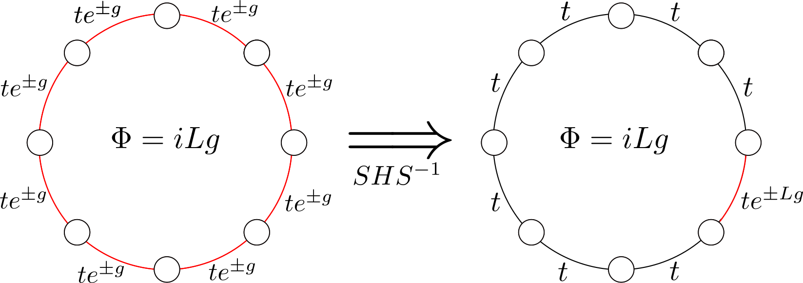
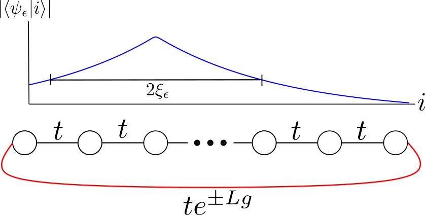
Now, let us consider the single-particle sector of the Hamiltonian (1) with open boundary conditions and ; we know that the states will be localized for any non-zero disorder strength . Let us consider an eigenstate at energy density 111For a given eigenvalue , the energy density is defined as the excitation energy of normalized by the bandwidth: Here , are maximum and minimum energies in the spectrum, respectively. in this open chain. This eigenstate will be localized at some lattice site - call it . Based on the discussion of gauge freedom above, let us introduce an imaginary flux by adding a term of the form to our system. Borrowing intuition from perturbation theory, we expect the non-hermiticity to become important when
| (3) |
where is the level spacing in the chain. See Fig. 2(b) for an illustration.
Using the localized state ansatz in (3) above, one finds the exceptional point for this eigenstate to be to leading order in . In other words, the tilt competes directly with the localization of the underlying hermitian Hamiltonian. This fact has been studied in detail by Hatano and Nelson for the non-interacting case Hatano and Nelson (1996); Hatano and Nelson (1998) and Hamazaki et al Hamazaki et al. (2019) for the interacting case. Hamzaki et al focused on the localization properties of the non-hermitian Hamiltonian (1) at nonzero , as opposed to using the real-complex transition to probe the localization properties of the underlying Hamiltonian (which is what the relation encodes).
The above argument, while suggestive, can be made precise. Specifically, let denote the single-particle eigenstate of the Hamiltonian (1) with open boundary conditions, and let be the exceptional point for the eigenstate in the closed chain with tilt (ordered by real part of the eigenvalue). Then one can show Heußen et al. (2021)
| (4) |
where is the “eigenstate localization length” (equivalently, the logarithm of the end-to-end Green’s function in the vicinity of ). While derived only for the single-particle sector of (1), Ref Heußen et al. (2021) showed that defining a length scale via (4) in interacting systems has the expected behavior of a localization length - namely, a finite-size scaling collapse of identifies critical parameters that agree with other numerical studies of finite-size MBL systems, and appears to diverge at the asymptotic transition. Thus, by searching for the exceptional points of the Hamiltonian (1) as we vary , we can directly probe the localization properties of the underlying Hamiltonian.
III Connection to Avalanche Model
In this section, we seek to connect the localization length to the length scale appearing in the avalanche model of delocalization. We do so in several steps.
III.1 Hermitian Avalanche Model
We begin with a brief review of the avalanche model of the localization-delocalization transition De Roeck and Huveneers (2017); Luitz et al. (2017); Thiery et al. (2018, 2017); Johri et al. (2015). In this picture, localized chains are coupled weakly to a thermal bath (or thermal sub-region of the chain), which can thermalize the sites bordering it. The new, larger, “effective” thermal bath comprised of the original bath and its thermalized neighbors can now thermalize the subsequent sites bordering it, and this can continue, triggering an “avalanche” that will either halt at some point - leaving the chain (partially) localized - or thermalize the whole chain.
To be more concrete, we consider the following toy model that captures the essential physics of such avalanches De Roeck and Huveneers (2017); Luitz et al. (2017). The system is a 1d chain of length , with sites being a thermal “bath”, and sites being many-body localized l-bits. The Hamiltonian is
| (5) |
where is the bath Hamiltonian (acting only on the bath sites), are bath creation/annihilation operators, are l-bit creation/annihilation/number operators, and are the single-particle energies associated with each l-bit. Additionally, is the base of exponential decay of the matrix elements coupling the bath to the localized part of the chain, with being the decay length of said matrix elements. This model neglects interactions between the l-bits, which are argued to induce only higher order corrections Luitz et al. (2017).
In the avalanche picture of delocalization, the eigenstate thermalization hypothesis (ETH) holds for a given l-bit if and only if it sucessfuly hybridizes with the bath according to Fermi’s golden rule Potirniche et al. (2019). Symbolically, this criteria amounts to the condition , where is the level spacing in the bath, and is a matrix element of the hopping between eigenstates of the unperturbed Hamiltonian . Assuming ETH for the bath, a typical matrix element between two energy eigenstates has the form , where the spectral function is a smooth positive function, and are the average and difference of the bath energies of the eigenstates, and is direct coupling between the bath and l-bit De Roeck and Huveneers (2017).
The l-bit most strongly coupled to the bath will be at site 1, and this l-bit hybridizes with the bath if . Should this l-bit hybridize, it will effectively become part of the bath; this (approximately) halves the level spacing and (approximately) leaves the spectral function unchanged: . One can now pose the hybridization criteria to the l-bit at site 2, with the level spacing of the “effective” bath half that of the original bath level spacing. Should the l-bit at site 2 hybridize with the bath, the level spacing will be further reduced by a factor of 2. This process continues at each site a distance from the bath so long as the hybridization condition
| (6) |
holds. Here, we’ve taken , with the level spacing of the original bath.
For the entire chain to thermalize, (6) should hold for all . Since the left hand side of (6) is monotonic, full thermalization can be determined by the behavior at the end of the chain (). Taking logarithms, full thermalization of the chain thus amounts to
| (7) |
In the thermodynamic limit, we can see this condition will always be satisfied for . We thus see the length scale controls the delocalization transition, which occurs at a critical decay length .
III.2 Non-hermitian delocalization & avalanches
In numerical studies of non-hermitian Hamiltonians with tilt whose counterpart is many-body localized, it has been observed that a non-hermitian MBL regime exists for small , and is eventually destroyed for large enough Hamazaki et al. (2019); Panda and Banerjee (2020). We conjecture that this non-hermitian delocalization occurrs by the same avalanche mechanism as in the hermitian case. That is, we propose that the imaginary vector potential helps couple ergodic grains to the rest of the chain in such a way as to successively delocalize neighboring sites of the chain.
Note that Ref Hamazaki et al. (2019) also argues that the real-complex transition roughly coincides with the non-hermitian delocalization transition in their numerics, and that the coincidence is exact in the thermodynamic limit. Under our conjecture, the exceptional points thus measure the location of this avalanche-based transition (i.e., ).
The conjecture that a non-hermitian avalanche drives the non-hermitian delocalization transition is a highly non-trivial statement, so we first verify it on a simple toy model. To that end, we consider the following non-hermitian version of the avalanche Hamiltonian:
| (8) |
This is the Hamiltonian (5), with the inclusion of a non-hermitian tilt. Note also that we include hopping from both ends of the bath, since the effect of can be gauged away for open boundary conditions.
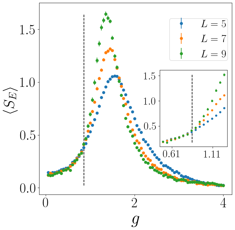
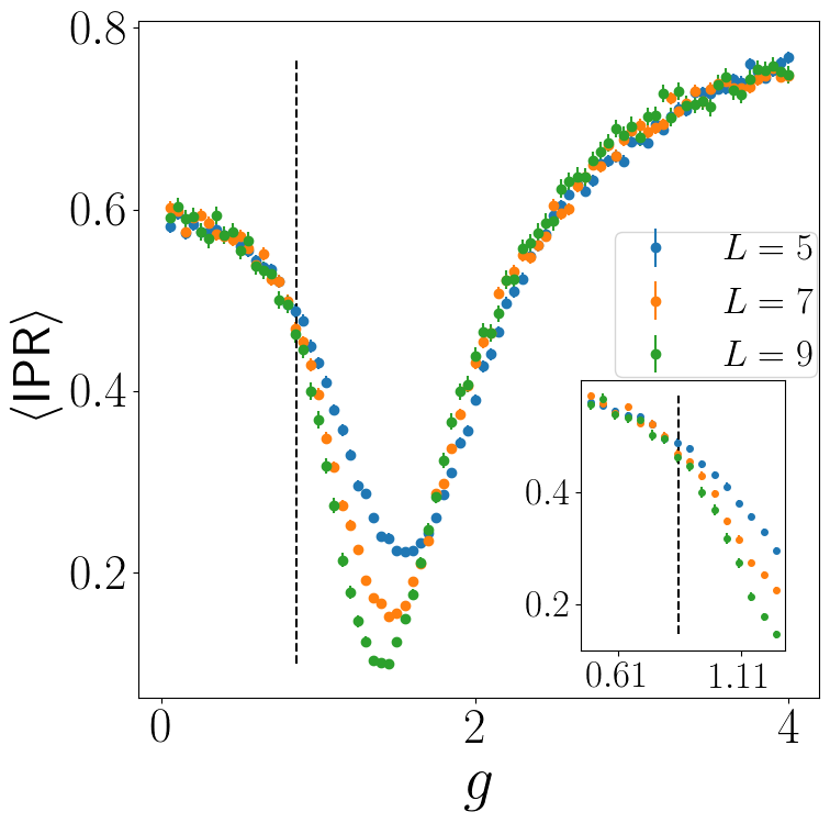
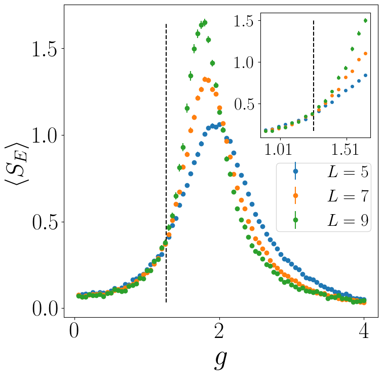
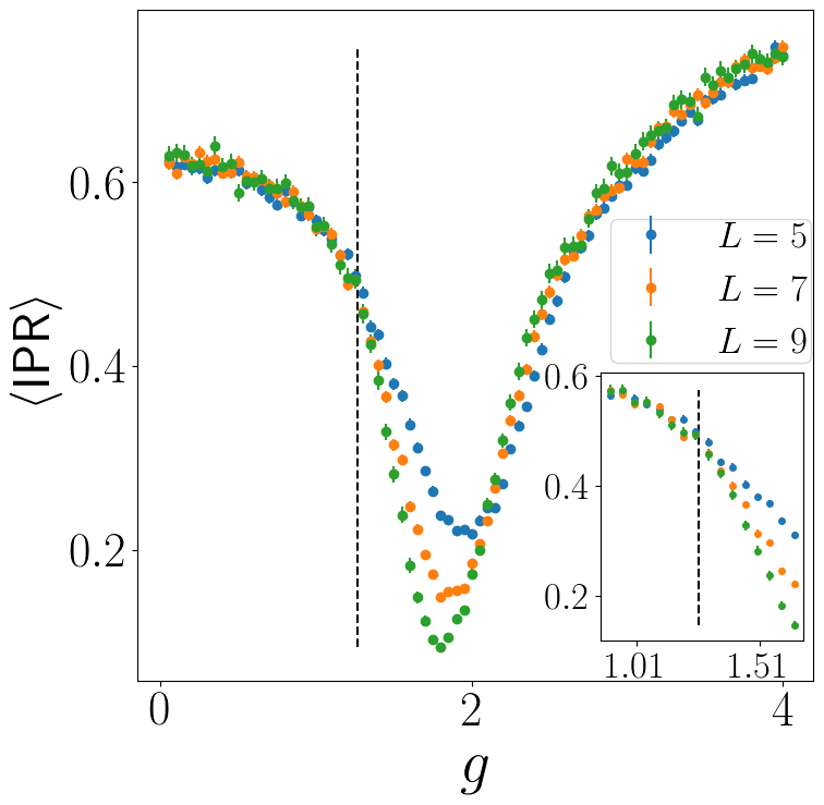
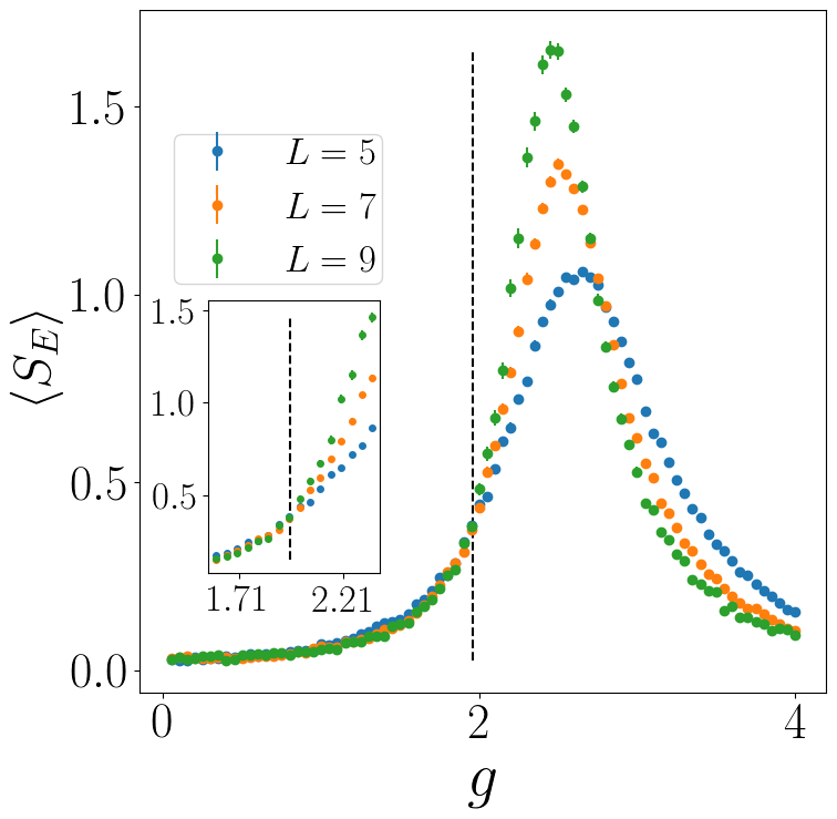
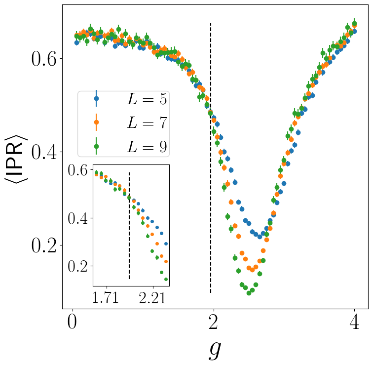
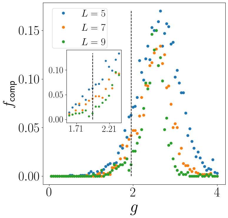
Figure 3 shows numerical results from diagonalizing the Hamiltonian (8) for several system sizes, in the half-filling sector, for . We can see a crossover in both the half-chain entanglement entropy and the inverse participation ratio from constant to increasing/decaying with system size (respectively), indicating a localization to delocalization crossover. These crossovers also occurr roughly at the value of we would expect from modifying the avalanche criteria (6) with , i.e. (with 222Note that we use the value of for the open chain here, since we expect from the non-interacting case that the exceptional points of the ring should probe the localization of the open chain formed by removing one of the bonds.). We also see similar crossovers for varying values of - see appendix C for additional examples. These results support the idea that a non-hermitian avalanche mechanism is driving delocalization in this model.
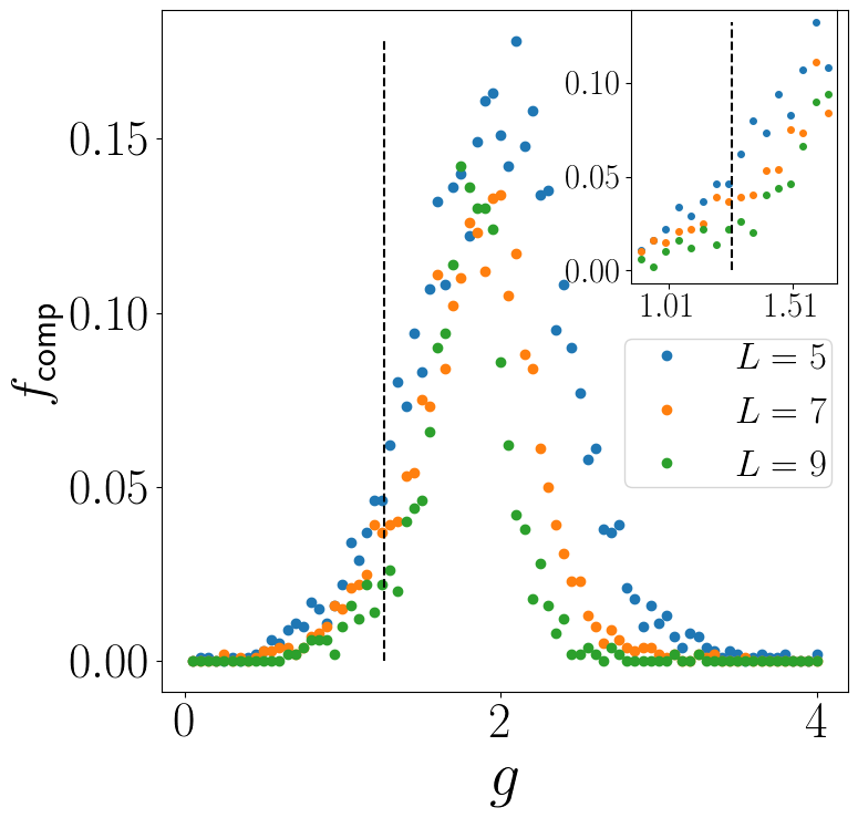
Figure 3(c) also shows the fraction of disorder realizations that have a non-real eigenvalue at energy density . Though there is no sharp transition or crossover, the window over which a non-zero fraction of disorder realizations have a complex eigenvalue overlaps with the crossover window observed in Figs. 3(a) and 3(b). This suggests that the real-complex transition may not only coincide with the many-body localization-delocalization transition (as previously suggested in the literature), but that it is consistent with a non-hermitian avalanche mechanism.
III.3 Mapping chain hamiltonians to avalanche hamiltonians
Having evidence that a non-hermitian avalanche drives the delocalization and real-complex transition in a simple toy model, we now would like to verify that the exceptional points in more generic Hamiltonians such as (1) are described by a similar mechanism. To do so, we need a way to explicitly connect such Hamiltonians to “avalanche” Hamiltonians resembling (8).
Let us consider a generic system comprised of a thermal bath/grain and a chain (which we take to be MBL). The Hamitonian is of the form
| (9) |
where and act only on the bath and chain (respectively), and couples the bath and chain subsystems. To bring this into the desired “avalanche” form, we need to re-express and in terms of -bits. In principle, this can be done straightforwardly by diagonalizing and performing a change of basis on . When using a generic diagonalization routine, however, it is not obvious how to extract the l-bit occupation numbers for each eigenstate. As the avalanche model relies on a cascade effect from thermalizing successive l-bits, we need to employ a diagonalization routine that allows us to access this crucial information.
To achieve this, we employ a mapping that combines the “displacement transformations” of Rademaker and Ortuño Rademaker and Ortuño (2016) with the principles of Wegner-Wilson Flow Pekker et al. (2017); Quito et al. (2016). Specifically, we construct and apply displacement transformations to eliminate individual off-diagonal terms in the Hamiltonian . We iterate this procedure, repeatedly eliminating the largest remaining off-diagonal term (as in the flow equation approach) until all such terms in are below some tolerance - see Appendix D for details. At the end, this procedure yields similarity transformations and that diagonalize and , respectively. We then apply these transformations to , which generates an avalanche-like series of terms involving hopping between bath eigenstates and the l-bits. Figure 4 illustrates this procedure schematically.

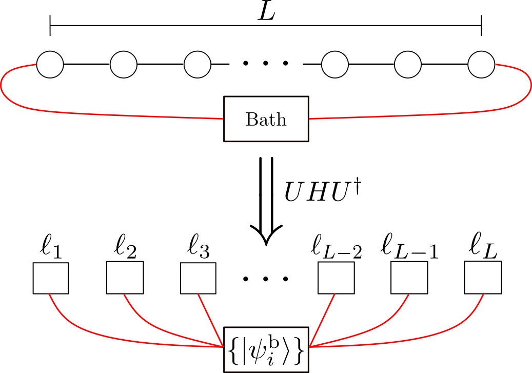
There are several important points about this procedure that we wish to emphasize. The first is that the transformation obtained from the Wegner-Wilson-flow like approach will well approximate the “near-optimal” mapping of basis states to l-bit configurations alluded to in Section I Pekker et al. (2017). Thus, we can read off the l-bit occupation numbers from the physical site occupation numbers in the original computational basis. The second is that by completely diagonalizing the decoupled bath/chain system - rather than diagonalizing only - we have access to the spectrum of the decoupled system. We can therefore label each l-bit/eigenstate hopping by its energy density in the uncoupled system, allowing for direct comparison with at the same energy density. The final key point is that, due to the gauge freedom, we can take to be hermitian without loss of generality. More specifically, we can gauge all of the flux onto the coupling Hamiltonian (i.e., the red bonds in Fig 4(b)), and perform our mapping on with . The transformations and will be unitary, and significantly easier to construct. The influence of the imaginary flux is also now simply a multiplicative weight for the various terms generated from by the change of basis (rather than being part of the transformations and , as it would be otherwise). We will leverage these last two points in the next two sections.
III.4 Applying the mapping
Let us now apply the mapping described in the previous section to a concrete model describing our system of interest. To that end, we take to be a GOE matrix (where is the bath size) and
| (10a) | |||
| (10b) |
where , are bath/chain fermion operators (respectively), are chain number operators, is the interaction strength, the are independently and identically drawn from a distribution characterized by strength , and is the length of the chain. Note that we have taken the bare hopping strength (c.f. the Hamiltonian (1)) to be unity, so that all quantities are in units of . Additionally, per the discussion of the previous section, we apply the mapping to a hermitian Hamiltonian without the vector potential ; we can restore the influence of by placing a flux onto the bonds in and out of the bath.
For each disorder realization, after applying the mapping, we need to extract the decay of matrix elements coupling each l-bit to the bath. To do so, we first separate the bath-chain coupling into couplings from the left and right end of the bath: and , respectively. In terms of the uncoupled eigenstates (where , are eigenstates of and , respectively), we obtain matrix elements:
We wish to extract specific matrix elements for each l-bit and energy density . To that end, we choose and above such that is the eigenstate closest to energy density in the uncoupled system. Then, for each l-bit , we define the amplitude via
|
|
(11) |
In words, we choose the largest (by amplitude) matrix element conecting to a state with the occupation of l-bit flipped and all other l-bit occupations the same - see Fig. 5(a) for a schematic example. Note that the choice of versus reflects the fact that hopping left (right) is enhanced (suppressed) when we eventually restore the imaginary vector potential ; hence, we choose the matrix element that will be enhanced by a factor of in each case above.
In the event that it is impossible to find such a hopping (if, for example, l-bit is unoccupied but the bath is empty), then we examine the eigenstate with energy density next closest to .


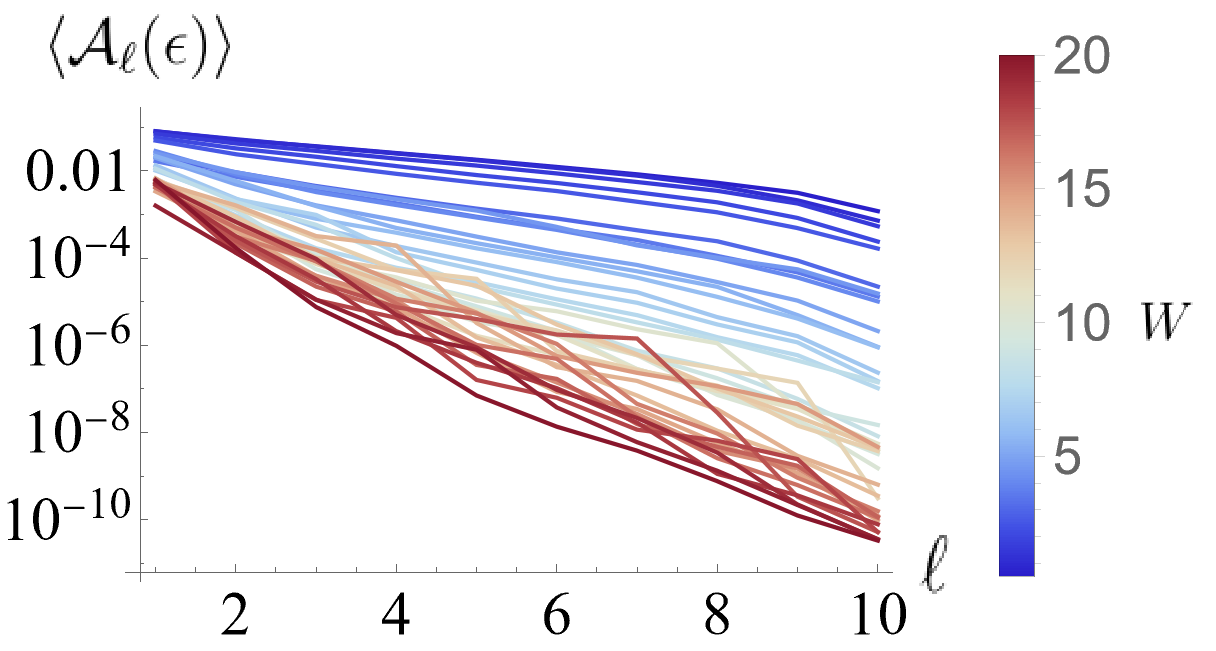
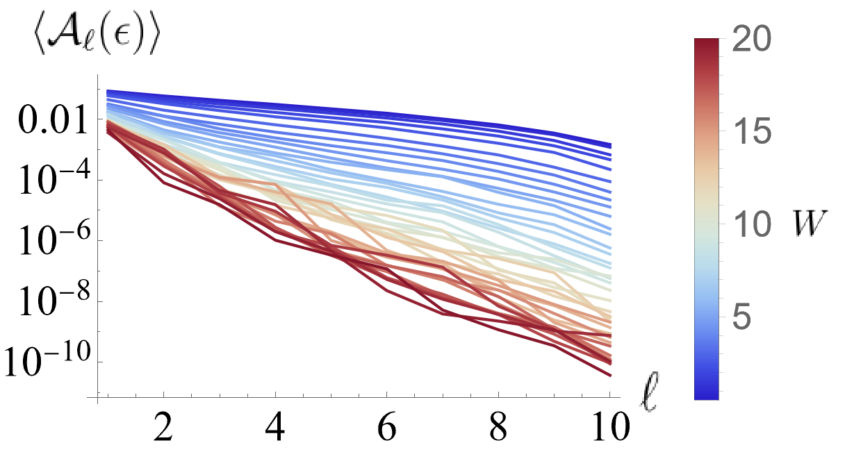
In the context of an avalanche mechanism, we are interested in studying how the couplings decay for each energy density. To that end, we assume without loss of generality that the are sorted in in descending order. The amplitudes , as well as their decay in , will generically be random (as they depend on the random disorder) - this is in stark contrast with the deterministic decay of the canonical avalanche model discussed in Section III.1. We do, however, observe that upon averaging over disorder realizations, the amplitudes decay exponentially in - see Fig. 6 for examples of how this is borne out in chains of size , , in the occupation sector 333The mapping described in section III.3 is computationally very expensive to run, so we use a smaller filling factor here in order to reach larger system sizes while keeping the Hilbert space dimension roughly fixed. We have verified that we attain qualitatively similar results at half-filling with smaller system sizes.. Consequently, the canonical avalanche model of Section III.1 emerges from our results upon disorder averaging.
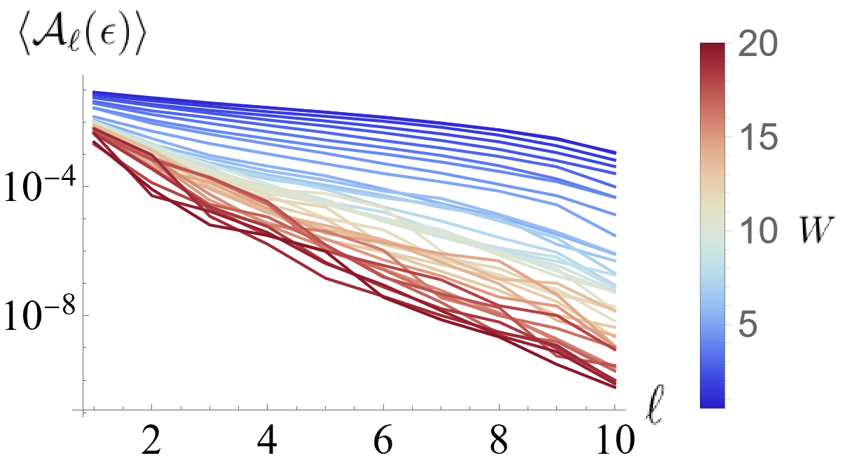
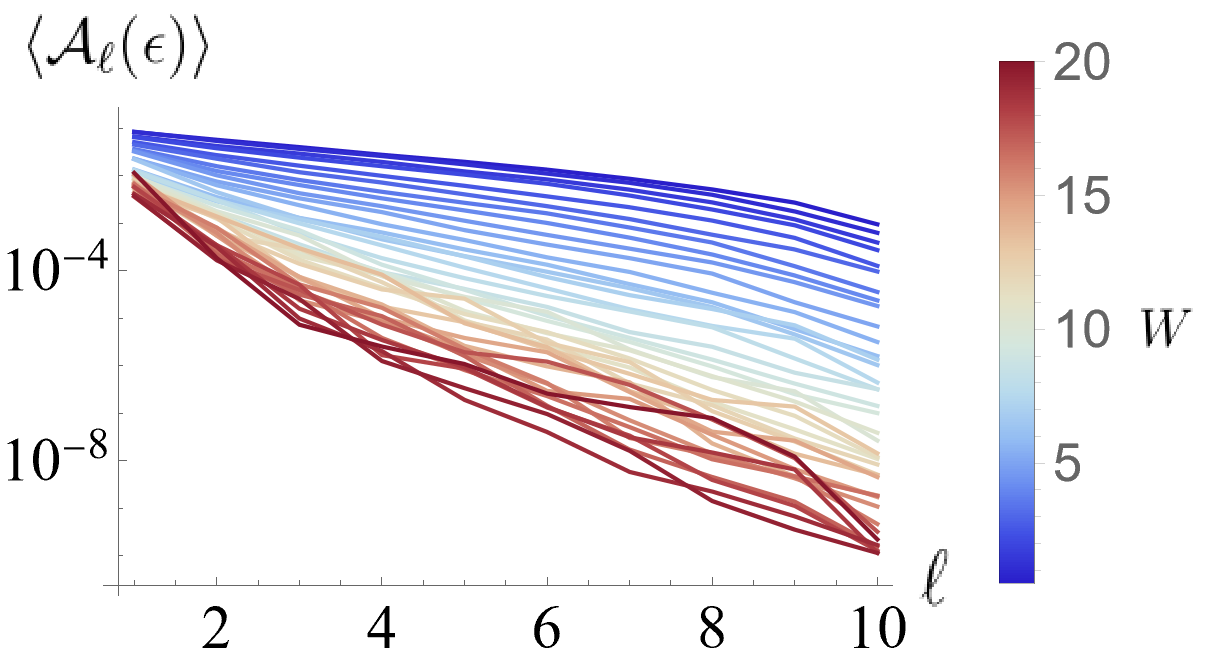
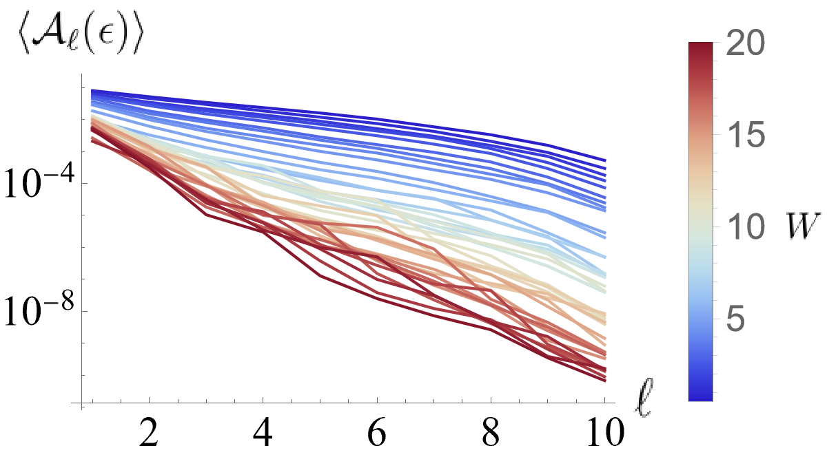
This mapping allows us to go beyond studying the disorder-averaged amplitudes - in particular, we have access to the distributions of and their decay in . To that end, we define the quantities
| (12) |
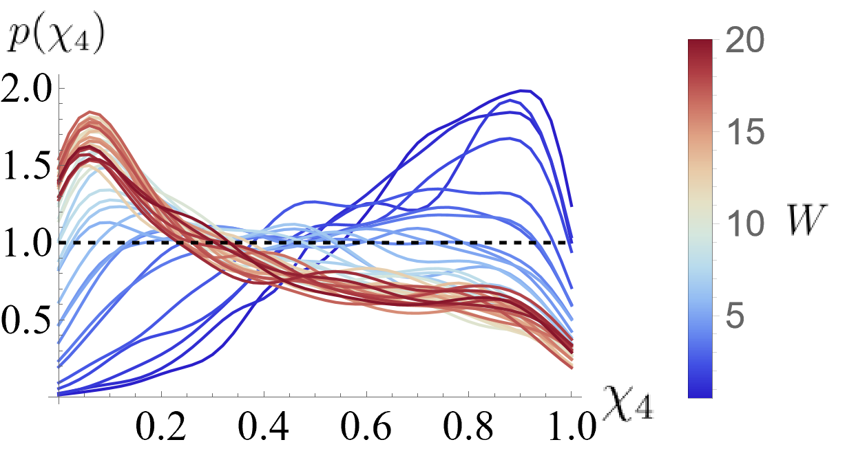
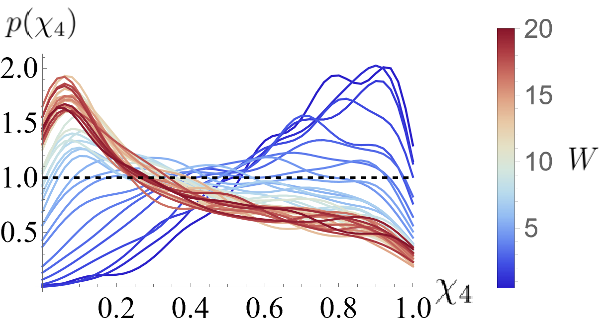
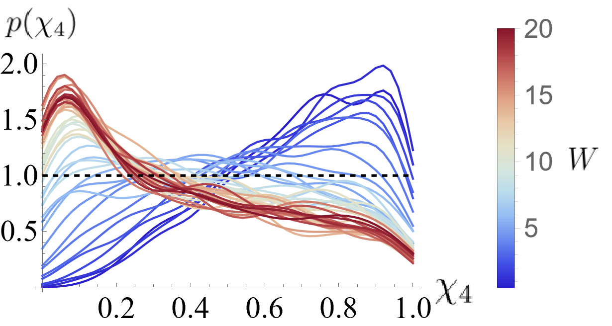
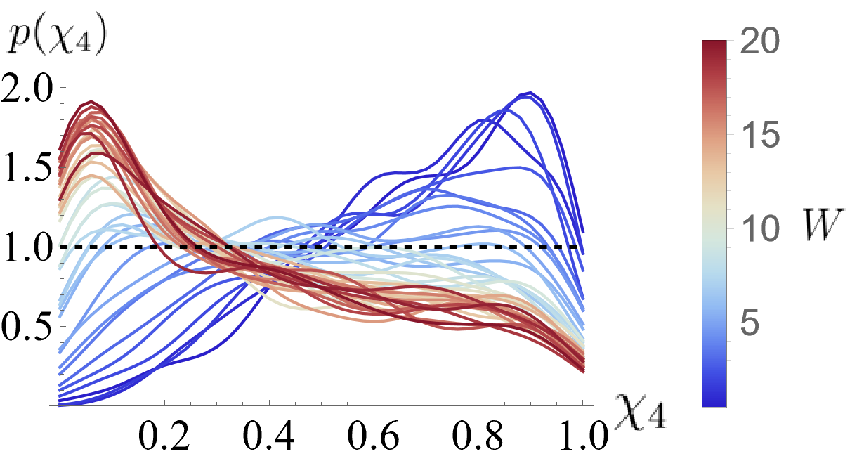
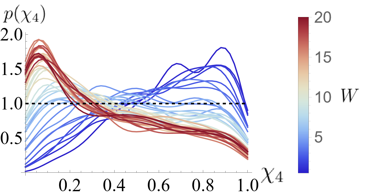
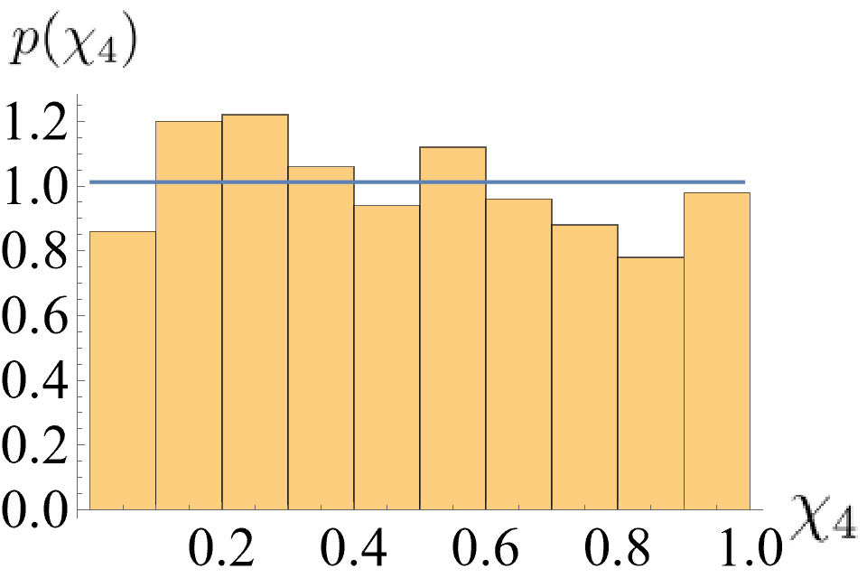
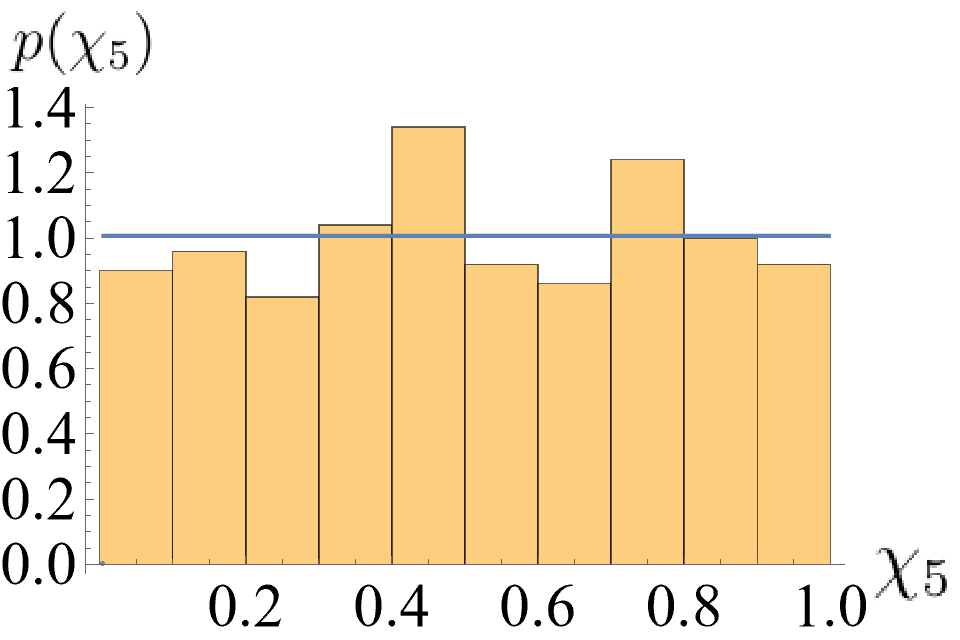
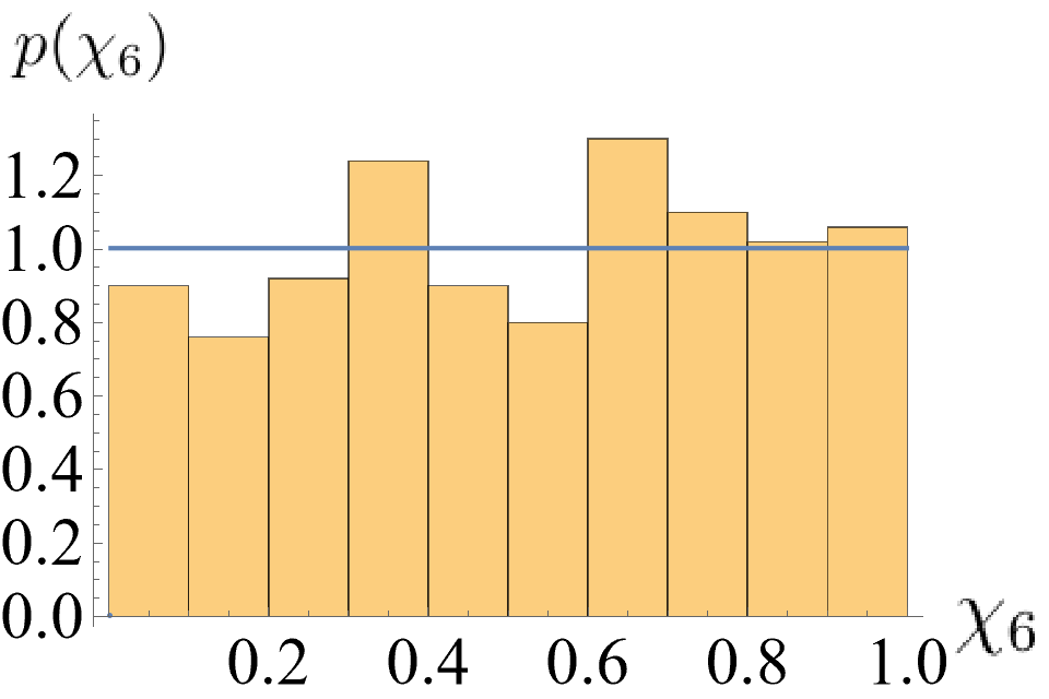
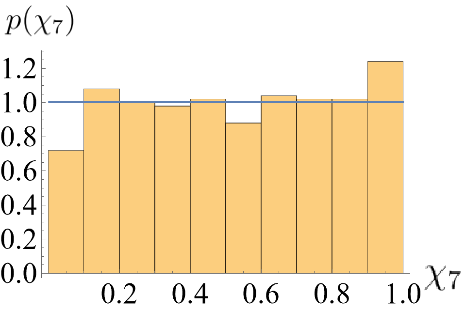
where we take . By construction, we have , with for each (as the are sorted to be monotonically decreasing in ). See Fig. 5(b) for a schematic illustration of the ’s. Such a decomposition amounts to replacing the deterministic decay in (8) by the random, energy dependent . The distributions of these show very interesting behavior as we bring the system from MBL to ergodic. Fig. 7 shows the observed probability densities of (with ) as we tune the disorder strength from deep in the MBL regime to ergodic. In the MBL and thermal regimes, the distributions are peaked near 0 and 1, respectively. This is consistent with the intuition that the amplitudes should decay slowly in the thermal regime and quickly in the MBL regime (which we observe to be the case on average in Fig. 6). Significantly, there is a window between the two extreme regimes where the distributions are approximately uniform. To make this statement more precise, we “fit” the numerically observed probability distributions in the vicinity of the MBL-thermal crossover, by minimizing the Akaike information over a large class of known continuous probability distributions. The Akaike information is defined as
| (13) |
where is the number of parameters in the model, and is the likelihood function. We choose to minimize the Akaike information, as it acts as an unbiased estimator for the expected Kullback-Leibler divergence (whereas the Bayesian information is a biased estimator), a standard measure for the information difference between two probability density functions Burnham and Anderson (2004). Fig 8 shows the numerically observed distributions of for several at the center of the spectrum for and (the critical point for the chain Hamiltonian (10a) - see Appendix B), along with the results of carrying out this fit. In all cases, the best-fit distribution is a uniform distribution on . Though we only show results for the center of the spectrum for , we find similar distributions at the transition throughout the spectrum, as well for . This observation that the amplitudes are uniformly distributed at the crossover will be key in the subsequent sections when we derive expressions for the distribution of at the critical point.
As a final note, the behavior of the distributions observed in Figures 7 and 8 is generic throughout the spectrum for (though the peak of the distributions at 0 in the MBL phase is less pronounced for ). For the largest and smallest values of , we do see (not shown) deviation from the behavior in Fig. 7; we expect this to be caused chiefly by finite-size and finite numerical precision effects. Going forward, we assume that the qualitative behavior observed in Figures 7 and 8 describes the asymptotic () behavior of the system, and we attempt to characterize our finite-size numerics by this expected behavior.
III.5 Connecting to
In section III.2, we found evidence that the non-hermitian many-body delocalization transition is consistent with a non-hermitian avalanche mechanism, and that measured the location of this transition, for the toy Hamiltonian (8). With the mapping of the previous two sections, we are now in position to test if an analogous relation holds for more realistic Hamiltonians (like the Hamiltonian (1)).
To that end, we take the Hamiltonian specified by (10b), add an imaginary flux , and compute for a variety of energy densities (see Appendix A for details on computing ). We do so for the same disorder realizations as shown in the previous section, so that we have both and for the same disorder realizations.
To connect to the , let us consider an avalanche proliferating in this chain. As remarked in the last section, the deterministic decay of hopping amplitudes in the toy model (8) must be replaced by the random variables . Because of this, the ratio of matrix element to bath level spacing (in analogy with (6)) is not necessarily monotonic, and we must examine this ratio for every l-bit to determine delocalization. We also incorporate the imaginary vector potential by enhancing each bond by a factor of (since, due to the gauge freedom, we can put all influence of onto the bonds connecting the bath and chain). Thus, the analogous condition to (6) (at energy density ) for all l-bits should read
| (14) |
In words, the flux must make up for the maximal “difference” between the (random) decay of the hoppings and the level spacing.
Based on the results of Section III.2, we expect that the exceptional points saturate this bound - that is, is exactly enough to cover all of these “differences”. We test this criterion numerically by computing
| (15) |
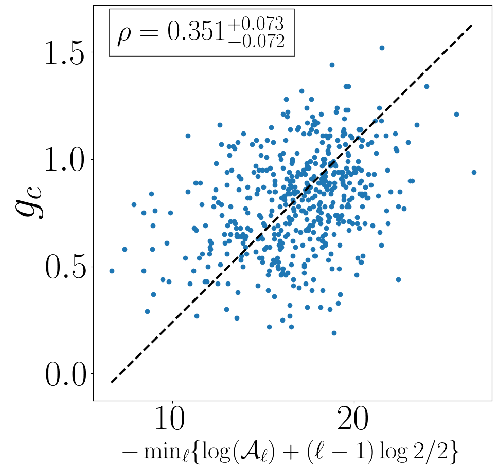
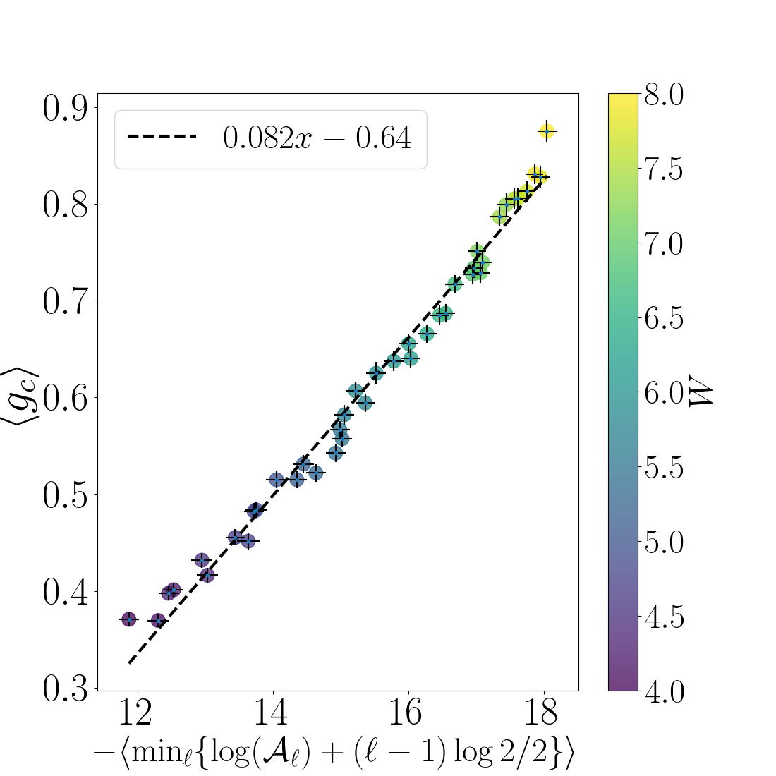
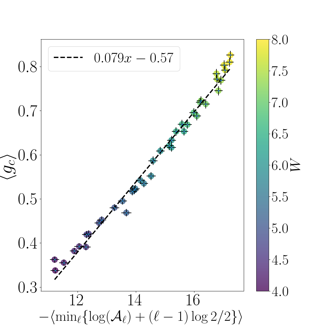
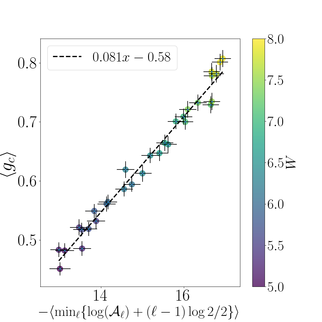
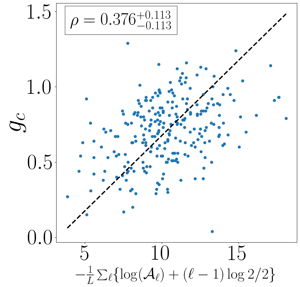
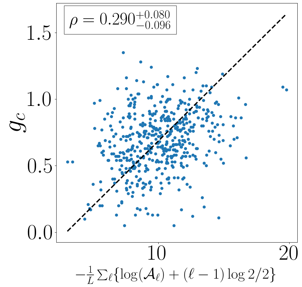
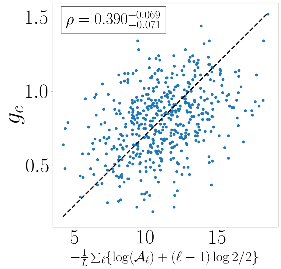
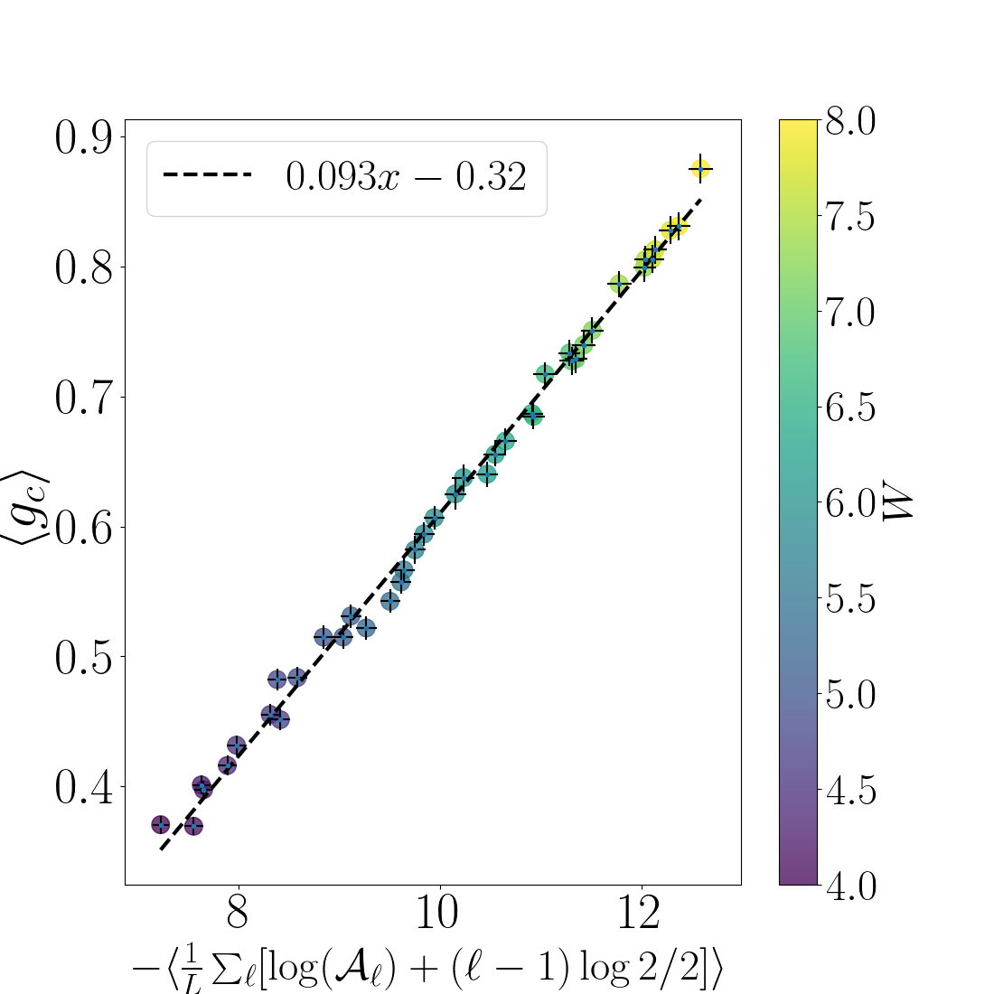
and for each disorder realization, and comparing the two. Visually, there is no clear cut trend, though the Pearson correlation coefficient suggests a weak linear relationship - see Fig. 9 for some example scatter plots. We observe a much clearer trend by averaging and over disorder realizations for multiple disorder strengths - see Fig. 10 for examples at the center of the spectrum. We are able to fit a line to the scatter plot of vs (where denotes a disorder average) - these fits are shown in Fig. 10 (and overlaid in Fig. 9), and Table 1 shows the resulting fit parameters (with uncertainties 444Uncertainties on the fit parameters were found via bootstrapping: for each disorder strength, we sample with replacement from the disorder realizations, average and , and perform a linear fit. The uncertainties on the slope and intercept are the the standard deviation of each quantity over 1000 such resamplings.). We find that the disorder-averaged data is well-fit by a line, and the slope agrees within error bars (at least at the center of the spectrum) with the expected value of (predicted by (14) with ). Curiously, the intercepts of these fits are non-zero. At present, we do not have an explanation for this, but we note in passing that the intercepts are roughly consistent with , which would correspond to a shift of about per non-bath site to . In any case, there is unmistakably a linear relationship between and , with (roughly) the correct slope of . This results support our conjecture in Section III.2, and the idea that the location of is given by saturating the avalanche criterion (14). This in turn means that the localization length captures the difference between the hopping decay and the level spacing.
In taking (15) as the “avalanche condition” determining , we are assuming that delocalization occurrs when all l-bits are delocalized by hybridizing with the bath. It is a worthwhile question to ask whether this is strictly necessary, and if delocalization of the system (indicated here by the eigenvalues acquiring a non-zero imaginary part) only requires a fraction of the l-bits to hybridize with the bath. Requiring, say, only out of l-bits to hybridize would entail replacing the minimum in (15) by the function that selects the ’th largest of the collection of values. In the extreme case of , the minimum in (15) should be replaced by a maximum; we find (not shown) that scatter plots analogous to Fig. 9 are very noisy and uncorrelated, and disorder-averaged fits analogous to those in Fig. 10 are very poor. Consequently, this extreme case is unlikely to capture the physics (unlike the minimum, corresponding to ).
It is not clear whether there even should be a universal value of for all disorder realizations. If varies from realization to realization, this could explain the non-zero intercepts in the linear fits of Fig. 10; the intercept could capture the (disorder-averaged) variation between the minimum and ’th largest value of across disorder realizations. To attempt to address this question, we repeat the analysis presented above with an average over l-bits, instead of a minimum - see Appendix G. There, we find comparable results to those we have presented in this section, and the linear fits generically have smaller intercepts. As averaging over l-bits does not fix a particular universal value of , this suggests that may indeed not have a universal value across disorder realizations. In spite of this - as we shall see in the next section - the avalanche condition (15) (i.e., taking ) appears to be the most successful in capturing the physics of in the original Hamiltonian (1) without a bath, so we primarily focus on this case moving forward.
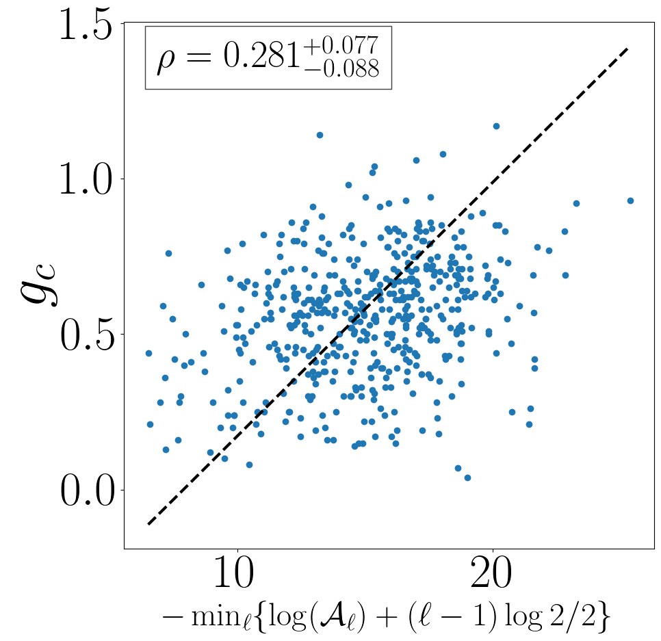
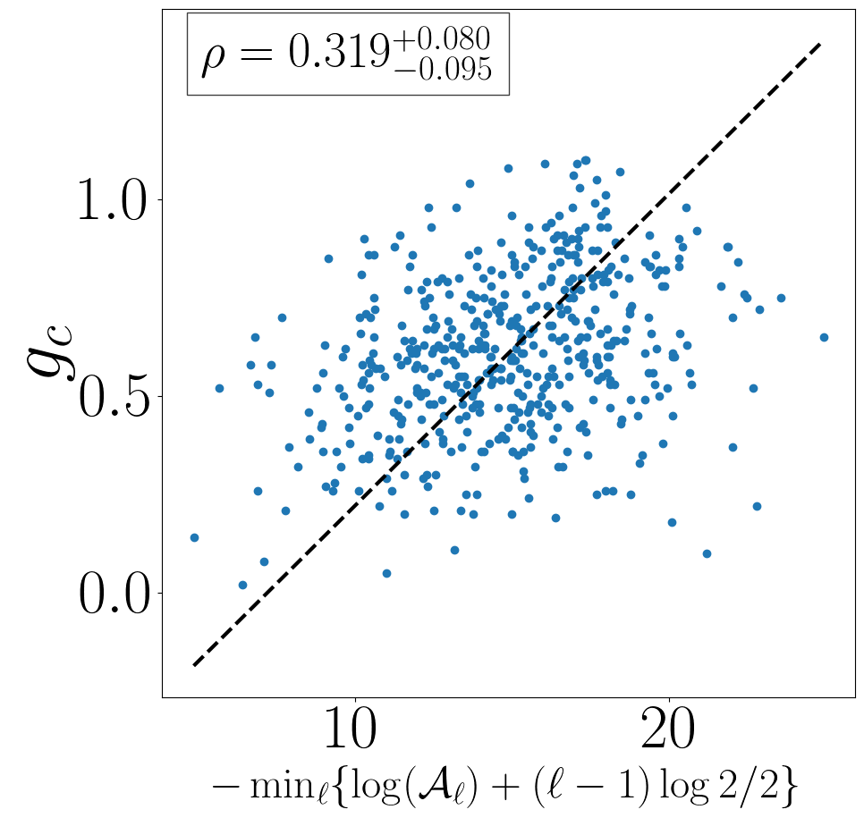
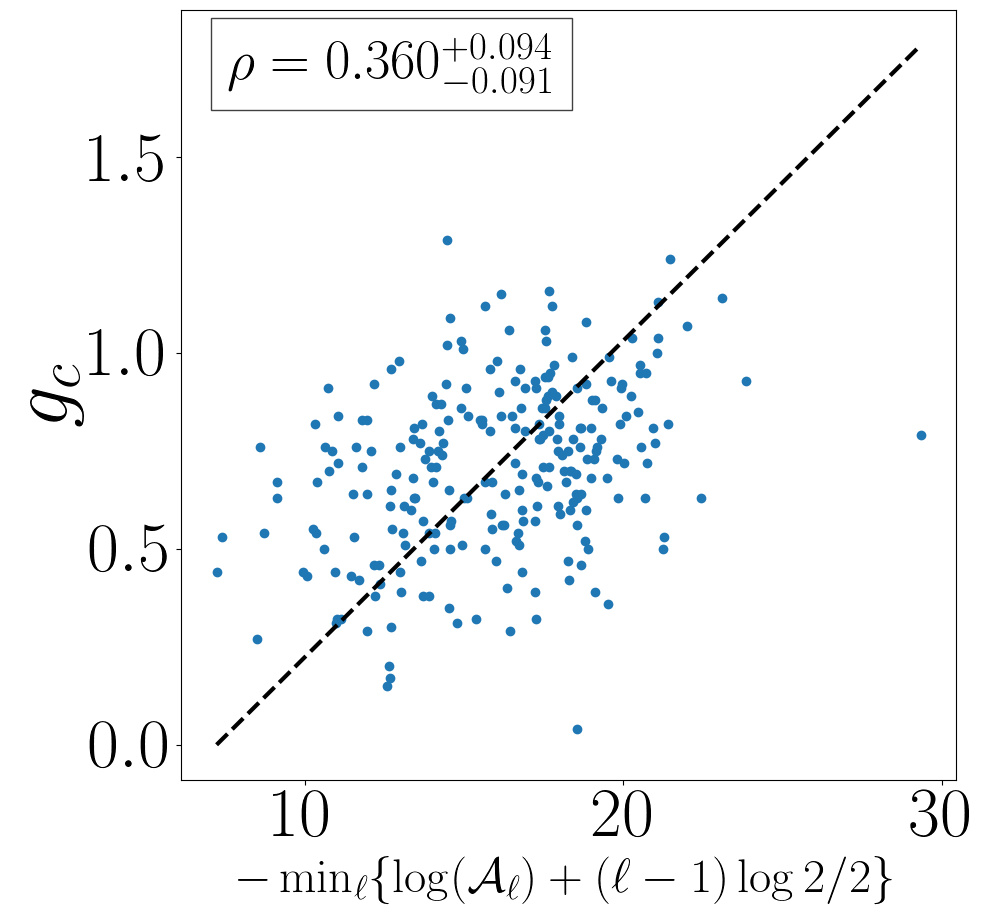
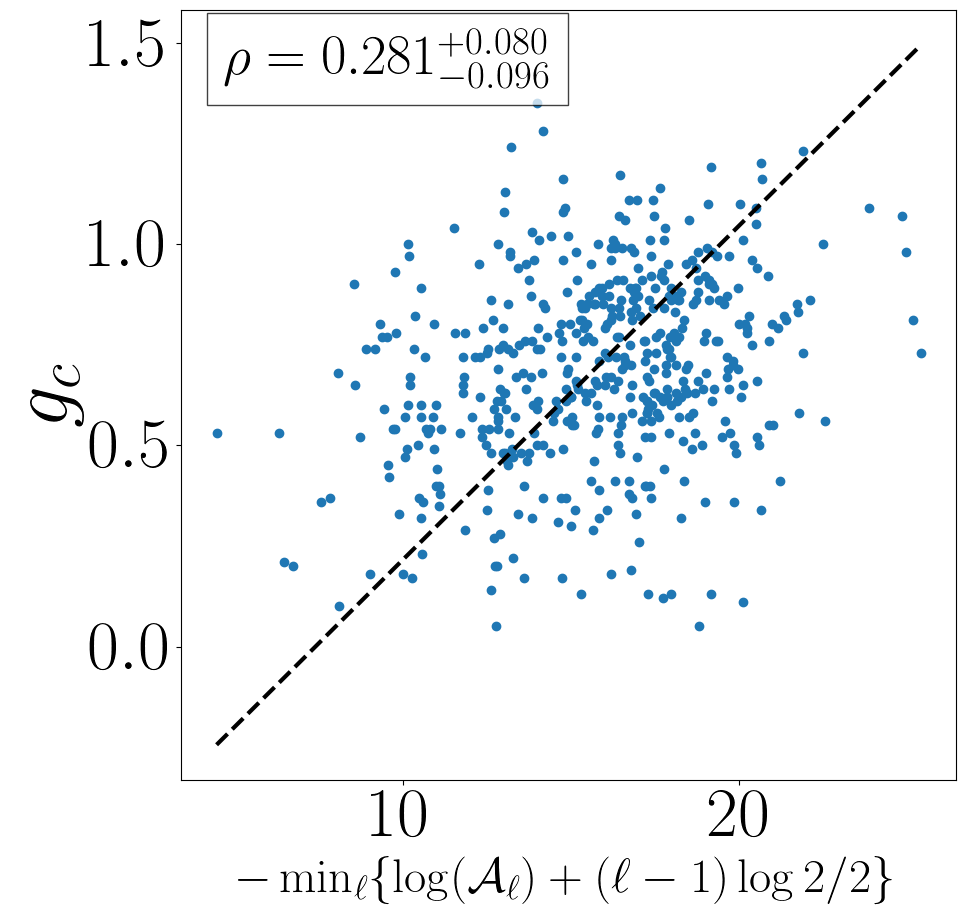
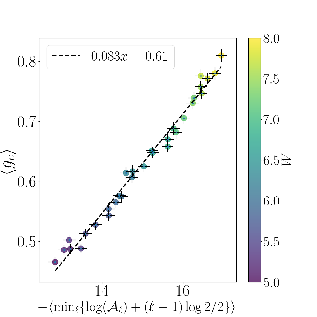
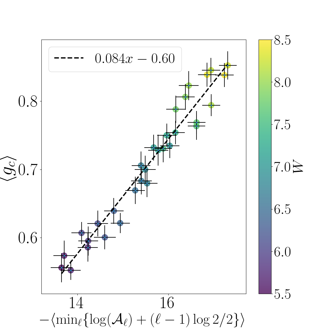
| Slope | Intercept | Slope | Intercept | Slope | Intercept | Slope | Intercept | Slope | Intercept | |
|---|---|---|---|---|---|---|---|---|---|---|
III.6 Single vs multi l-bit flips
Before moving on, we address a key aspect of the definition (11) of the amplitudes : the fact they are derived only from considering single l-bit flips.
At first glance, such a definition may seem too restrictive; namely, that by considering only single l-bit flips, we are missing the dominant processes by which the system relaxes (as observed, e.g., in Ha et al. (2023)). We find, however (not shown), that extending the definition of to include all hoppings that flip l-bit yields quantitively worse results - in the sense that scatterplots akin to Fig. 9 show near-zero Pearson correlation and linear fits akin to Fig. 10 yield the wrong slope. Our numerics are thus more consistent with an avalanche mechanism that propagates via single l-bit flips only.
This is not to say that our results suggest that multi l-bit flips are not important to the finite-size MBL regime or the avalanche mechanism - the growing consensus in the literature is that they very much are Gopalakrishnan et al. (2015); Villalonga and Clark (2020a, b); Garratt et al. (2021); Crowley and Chandran (2022); Morningstar et al. (2022); Long et al. (2022); Garratt and Roy (2022); Ha et al. (2023). Rather, we suspect the primary reason behind this apparent discrepancy is the fact that our imaginary vector potential couples to charge. The real-complex transition we detect thus corresponds to delocalization of charge, rather than entropy or energy (which other studies such as Ha et al. (2023) are sensitive to). Correspondingly, our imaginary vector potential may not be sensitive to charge-neutral processes that thermalize the system, which based on our numerics seem to coincide with processes that flip multiple l-bits at a time.
IV Distributions at the MBL crossover
We have sucessfully connected the localization length to the length scale appearing in the avalanche model. We now seek to leverage this relationship to predict the distribution of (with respect to disorder) - the distribution of then follows as the inverse distribution, per the relationship . We focus here on the distribution at the MBL-thermal crossover, as we have an analytic form for the distribution of the amplitudes (based on the observations of Section III.4).
Based on the results of Section III.5, we consider the following generalized relation between and the ’s:
| (16) |
where is the total flux through the system, the number of l-bits in the system, and , where is the on-site Hilbert space dimension (in fermionic models, ). We also allow for an offset , based on the results of Section III.5. Note that we have written the relation in terms of a maximum here, to ease analytic computation of the distribution.
Let us assume this relation for holds for each disorder realization (i.e., we neglect the noise observed in Fig. 9), and let denote the cumulative density function for given by this relation. As observed in Section III.4, we have with uniformly distributed on at the MBL crossover. Using this, we arrive at the following form for the cdf:
|
|
(17) |
where - see Appendix E for details on the derivation of this result. Crucially, we note here that the derivation in Appendix E assumes the are independently and identically distributed. This is not strictly true, as the distributions of do vary in (as remarked in Section III.4), and all the arise from the same disorder realization, and are thus almost certainly correlated. We neglect these two facts here.
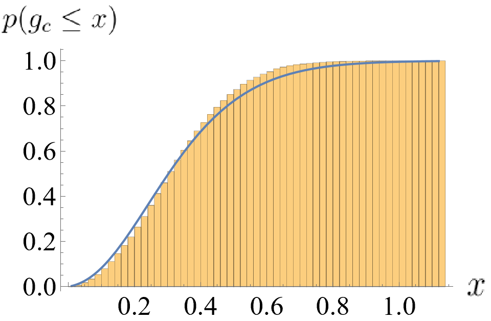
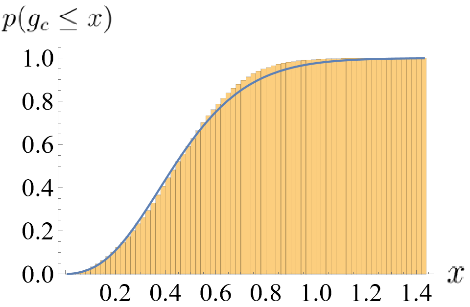
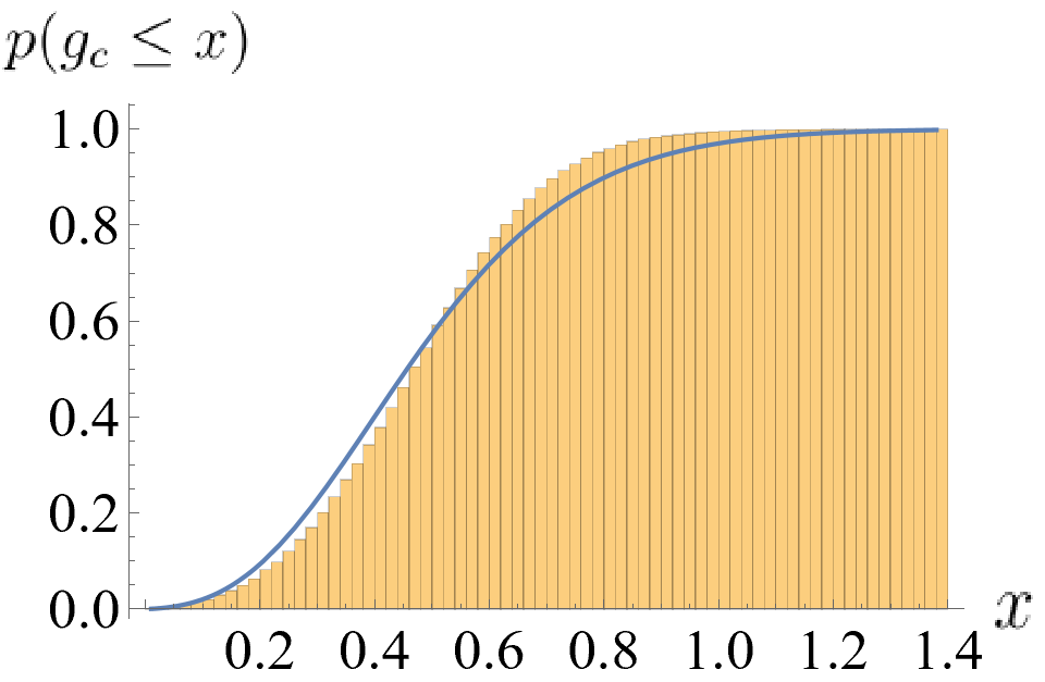
We now would like to see if the analytic distribution (17) describes the distribution of ’s (and thereby ’s) at the MBL crossover in the original model, (1). To that end, we compute the histogram of at the (energy-resolved) critical disorder strength identified from finite-size scaling (see Appendix B). We cannot compare the numerically observed distributions directly to (17), however, as the Hamiltonian (1) doesn’t explicitly include a thermal bath/grain. The size of the bath is thus itself also a random variable; we account for this by modifying (17) to a mixture distribution of the form
| (18) |
with , . In this distribution, is the probability the bath/thermal grain is of size , and is the CDF of conditioned on the bath being size . Such a distribution follows from the law of total probability applied to the CDF of .
We fit a mixture distribution of the form (18) to the numerically observed CDF. We do so by computing a kernel density estimator of the numerically observed CDF (using a Gaussian kernel), sampling this estimator at various points , and numerically minimizing the squared error
| (19) |
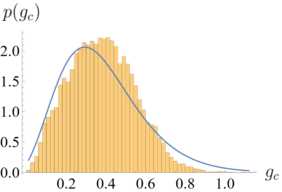
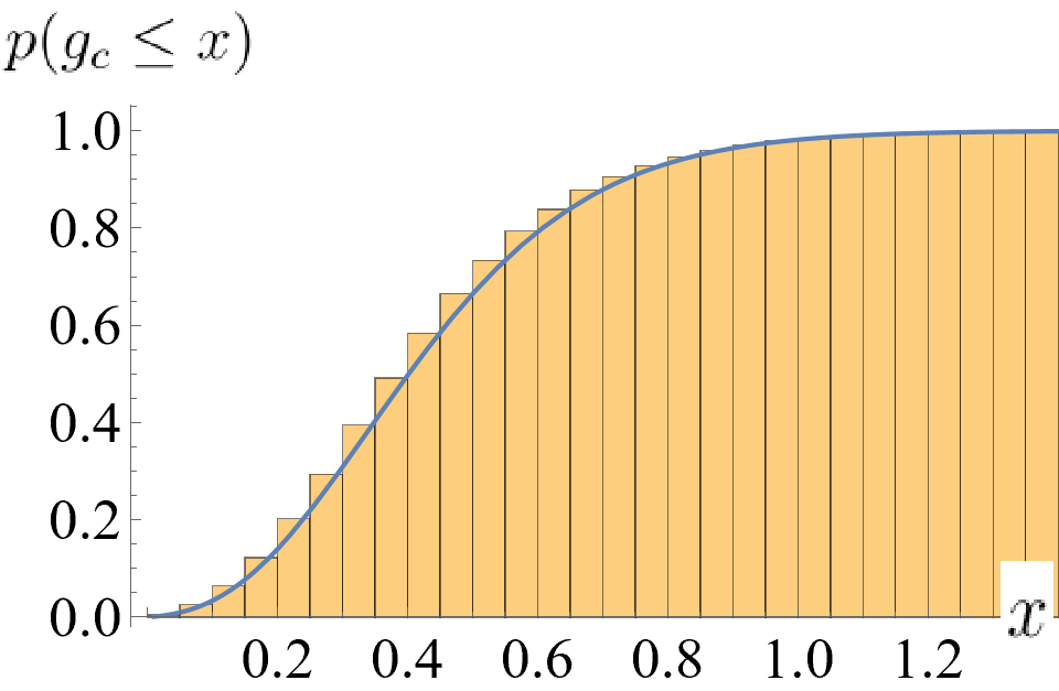
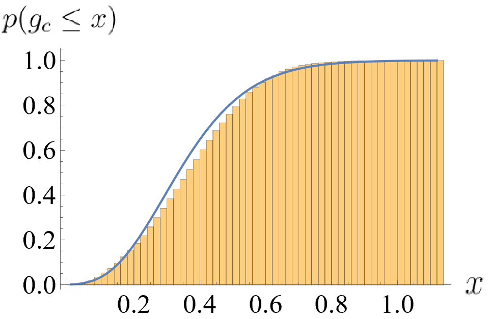
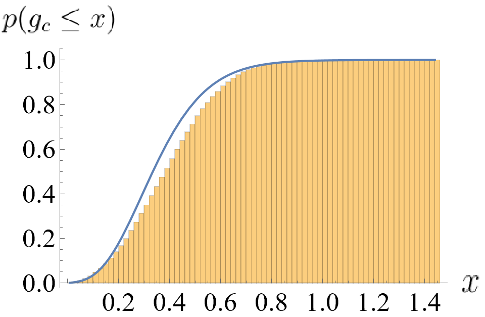
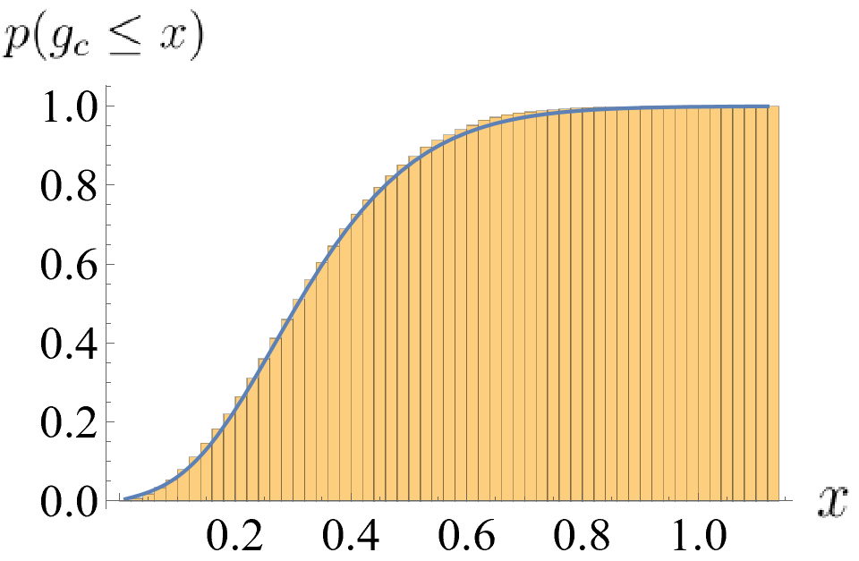
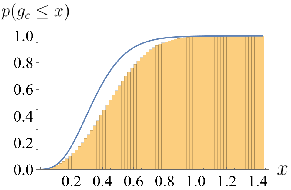
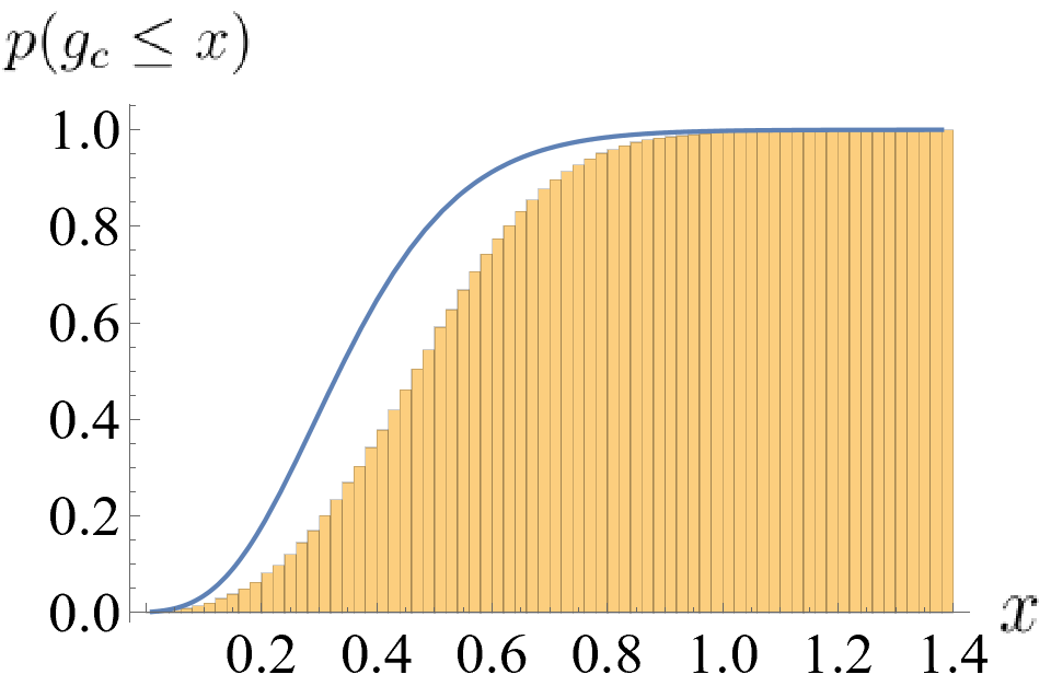
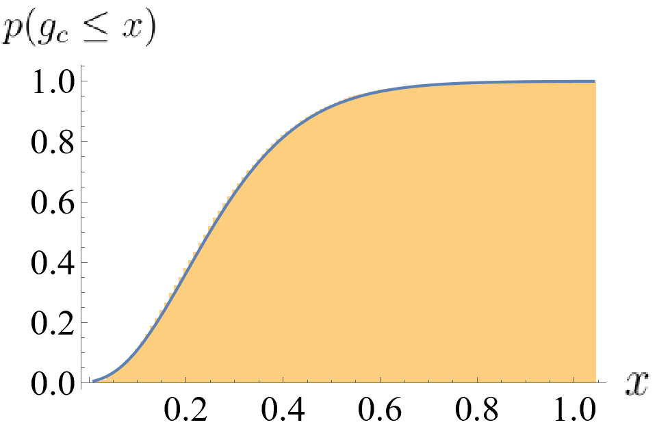
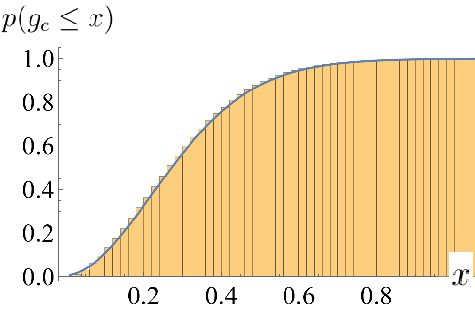
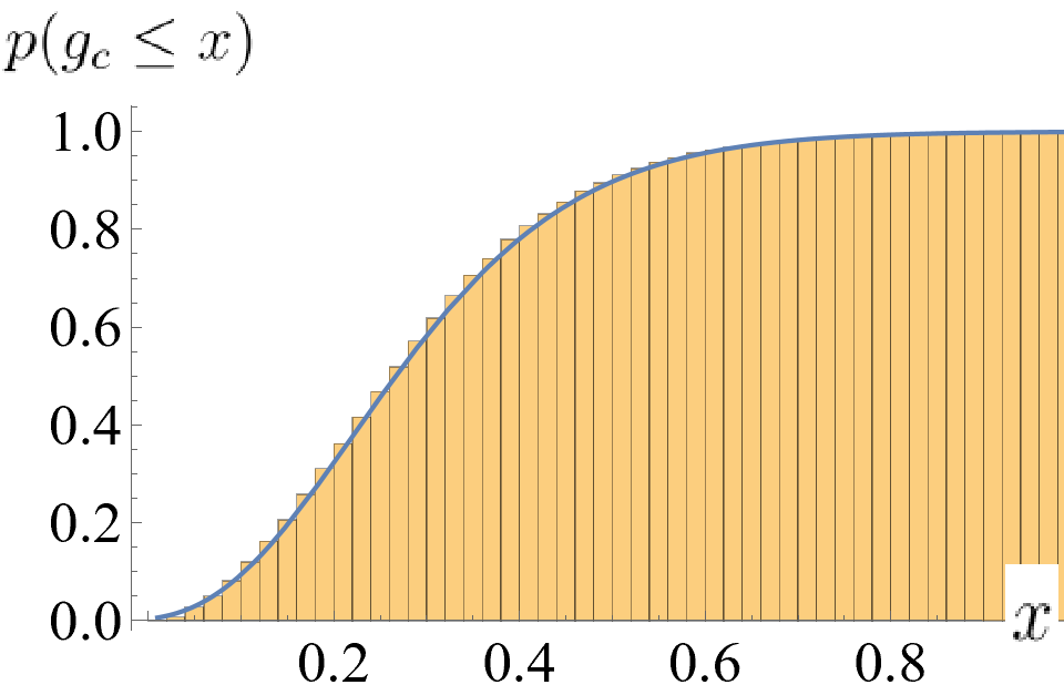
subject to the constraints , . The results of this fit at the center of the spectrum are shown in Fig 11. We see good overall agreement between the observed CDF and the fitted mixture distribution, though the fitted distributions have longer tails than the observed distributions (as evidenced by the slower approach of the CDF to 1 - see also Appendix F). This suggests that the distributions of at the critical point are well-described by an avalanche-like picture of delocalization (which gives rise to the distribution (18)). The distribution of , obtained by computing the inverse distribution of (18), thus contains information about the distribution of the hopping amplitudes .
Curiously, we find all the fits have ; the offset does not appear to play a role in the physics without the bath. In light of the discussion at the end of the previous section, the lack of offset would suggest that all l-bits () must hybridize when there is no explicit bath in the system. In Appendix G, we derive an analytic distribution of assuming an average avalanche condition and perform similar fits; the agreement between fitted and numerically observed distributions is not as good for the average avalanche condition (especially at larger interaction strengths). This further suggests that the physics in the system without a bath is captured by requiring all l-bits to hybridize ().
The mixture distribution defined by (18) contains free parameters (the ’s, with one of them fixed by , and ). As a result, the agreement seen in Fig 11 appears not too surprising, despite the fact that this discrete set of parameters is paramterizing a continuous distribution relying on thousands of disorder realizations. However, one must keep in mind that the ’s represent how the system partitions itself into localized and ergodic subregions. It is this information that parameterizes the distributions , and this information is, in principle, calculable by other means (which could eliminate the ’s as fit parameters entirely). Indeed, in all the fits we show, only a subset of the fitted parameters (2 in the case of Fig. 11, 2-4 for the fits shown in the Appendices) are non-zero, and the indices of the non-zero ’s seem to increase with increasing interaction strength . This is consistent with the idea above that the ’s are not actually free, but rather determined by another unknown function: the distribution of sizes of thermal inclusions in the system. Determining this distribution, especially for small system sizes where one must account for resonances, is beyond the scope of our current work, so we instead treat the ’s as fit parameters.
As a final remark, we note that the fit quality of the mixture distribution (18) is even better towards the band edges - see Appendix F for examples and discussion.
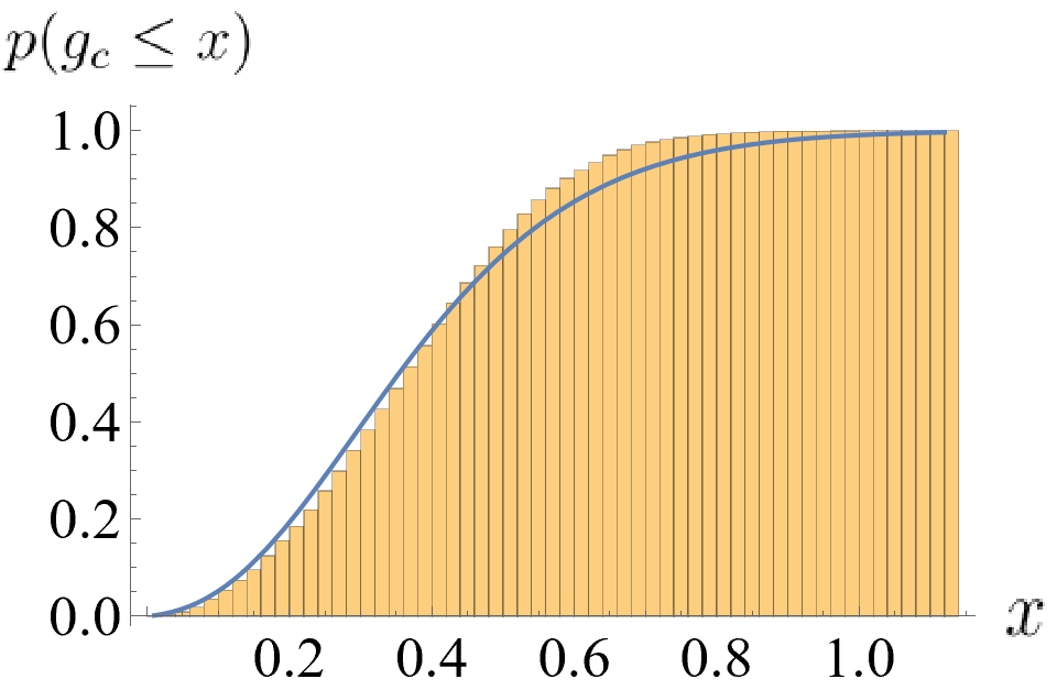
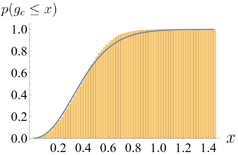
V Conclusion & Discussion
We have shown how to connect a localization length , defined by introducing an imaginary vector potential to a disordered chain of interacting fermions, to the length scale characterizing the decay of matrix elements in the avalanche model of delocalization. We have also derived an analytic form of how the ’s are distributed at the MBL crossover in finite systems, and shown that this form describes well the observed histograms. The distributions of at the crossover, which can be derived from those of , thus contain information about the distribution of avalanche-like hoppings, giving insight into the avalanche mechanism at the finite-size crossover.
Determining , while computationally difficult, has the advantage of not requiring one to explicitly construct the l-bits. That is, a given with a fixed disorder realization has a well-defined , and thereby , for each energy density . Though our numerical verification of saturating the avalanche condition (14) made use of a particular construction of the l-bits, the agreement of the numerically observed histograms to our fitted CDFs (18) suggests the form of avalanche criteria for does not depend on how the l-bits are constructed. This method thus allows one to obtain information about the localization of the underlying Hamiltonian whilst sidestepping issues with defining the l-bits.
The connection of to the localization properties of the underlying system relies on the proliferation of avalanches enhanced by the imaginary flux through the system. It is therefore an intereresting question to ask how a defined analogously for “clean” systems differs, as there are no rare regions driving thermalization in these systems. The recent wealth of work on the crucial role of many-body resonances in finite size MBL systems Gopalakrishnan et al. (2015); Villalonga and Clark (2020a, b); Garratt et al. (2021); Crowley and Chandran (2022); Morningstar et al. (2022); Long et al. (2022); Garratt and Roy (2022); Ha et al. (2023) also raises the question of how is connected to these resonances; after all, avoided crossings are generically expected to give rise to exceptional points when the parameter space is expanded to the complex plane Heiss and Sannino (1990); Luitz and Piazza (2019). In particular, it is worth asking how could be used to probe the statistics of many-body resonances in the finite-size MBL regime (and how such a connection affects the distributions we derived in Section IV). Additionally, in light of the discussion of Section III.6, it would be interesting to adapt this non-hermitian technique such that the real-complex transition corresponds to a non-zero information current. This (presumably) would make this non-hermitian method sensitive to the destabilizing charge-neutral processes alluded to in Section III.6, and would be an interesting comparison with the results derived here.
Finally, though we introduced the l-bits and the mapping of Section III C primarily as an intermediate step to connect to the avalanche model, the mapping and the numerical results in Section III D open several potential avenues of future work. Among other questions, the significance of the distributions of the - especially being uniformly distributed at the MBL-thermal crossover - is worthy of additional study. The implications of these distributions for the properties of the l-bits is particularly interesting.
Acknowledgements.
LO and GR thank David Huse for useful discussion regarding the distinction between single and multi l-bit flips when defining . LO also thanks Christopher David White for his guidance and advice during the early stages of this project, as well as Dan Borgnia for useful discussions. GR is grateful for support from the Simons Foundation as well as support from the NSF DMR grant number 1839271, and from the IQIM, an NSF Physics Frontiers Center. This work was performed in part at Aspen Center for Physics, which is supported by National Science Foundation grant PHY-1607611.Appendix A Numerical Procedure for Obtaining
Here, we briefly summarize our numerical procedure for obtaining the exceptional points .
For a given instance of a Hamiltonian (i.e., a fixed disorder realization), the exceptional point at energy density is defined as
| (20) |
where is the eigenvalue at energy density . The length scale is then defined by - from here on we refer to as the localization length.
For finite-size systems, the energies are discrete, and we must consider the eigenvalue closest to energy density , given by
| (21) |
where is the spectrum of , and , are the eigenvalues with the maximal and minimal real parts (respectively).
To find numerically for a fixed disorder realization, we repeatedly increment by a fixed step (which we take to be .01), exactly diagonalizing the Hamiltonian at each value of , until is larger than some tolerance (which we take to be ). Note this numerical approach differs from previous studies that examine all eigenvalues within some energy window to determine . We choose to sample only one state per disorder realization to sidestep subtleties involving correlations of eigenvectors from the same disorder realization Rodriguez et al. (2011). We have verified that this approach gives the same disorder-averaged results as averaging over an energy window.
Appendix B Identifying the MBL crossover via finite-size scaling
In this Appendix, we show finite-size scaling collapse on the disorder-averaged localization lengths to identify the location of the (finite-size) MBL-thermal crossover for the Hamiltonian (1). We find results in good agreement with those of Heußen et al. (2021).
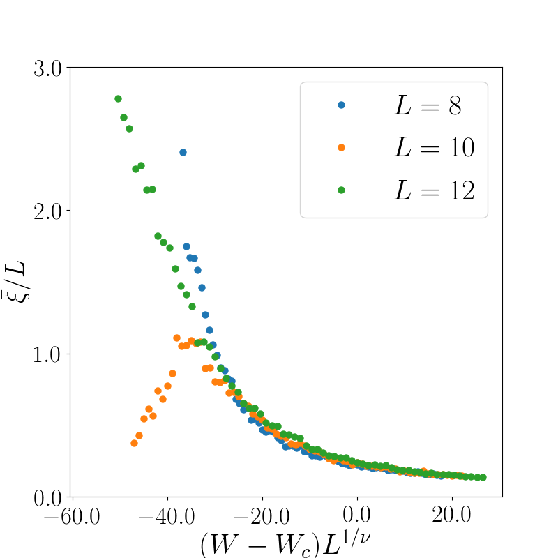
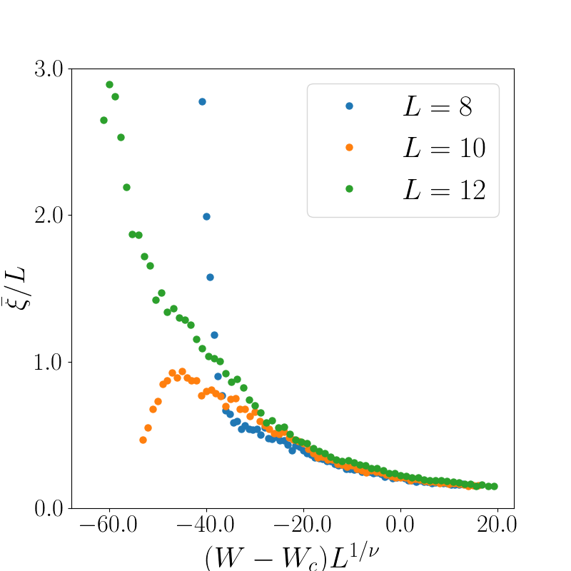
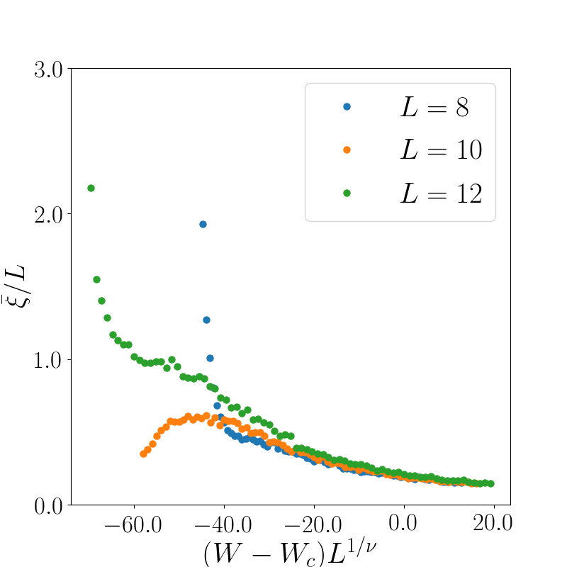
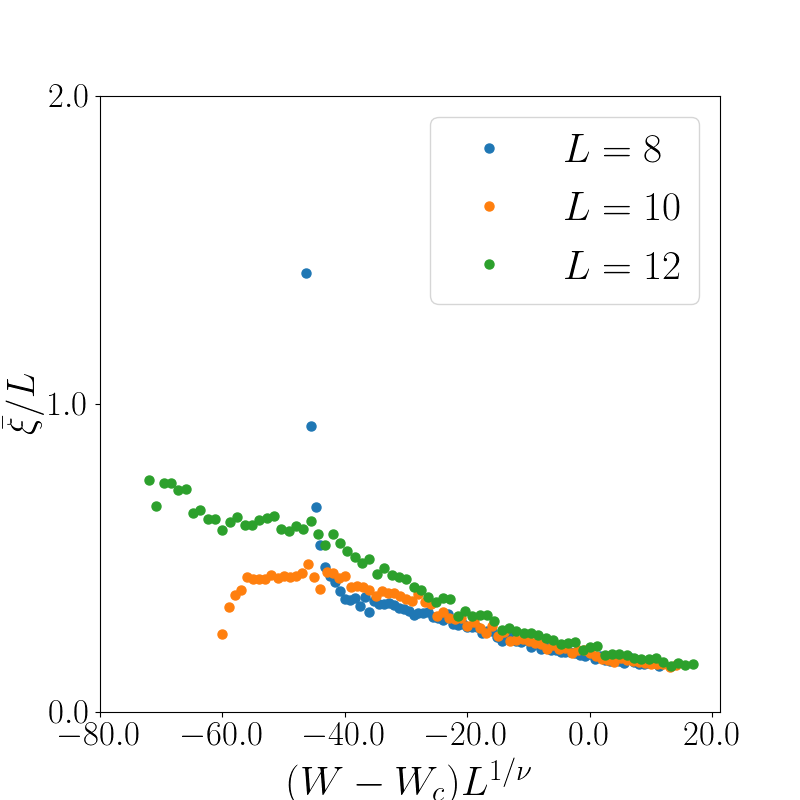
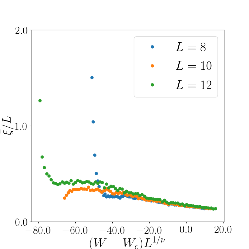
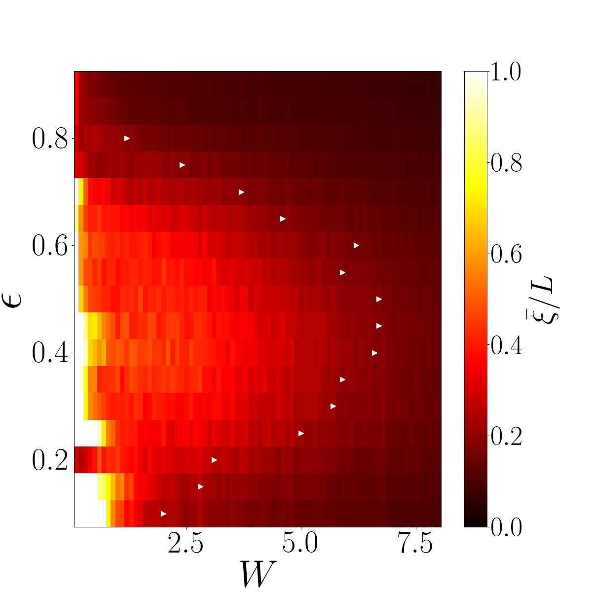
To that end, we compute (as described in Appendix A) for the Hamiltonian (1), with bare hopping (making it the energy scale of our system) and on-site disorders sampled from a uniform distribution . Figure 12 shows finite size-scaling of (where denotes a disorder average) at the center of the spectrum () in the half-filling sector. We examine a variety of interaction strengths , at system sizes , and average over 200 disorder realizations. We obtain good collapse of the data to the form
| (22) |
and in all cases find critical exponents . The resulting phase portraits in the - plane are shown in Fig. 13, with the transition points identified from the finite size scaling marked. We see the transition points capture the change from large (order of system size) to small localization length as we tune the disorder strength. The shape of the mobillity edge in the phase diagram also mirrors that of other finite size studies Luitz et al. (2015), and the critical disorder strengths agree well with Heußen et al. (2021) .
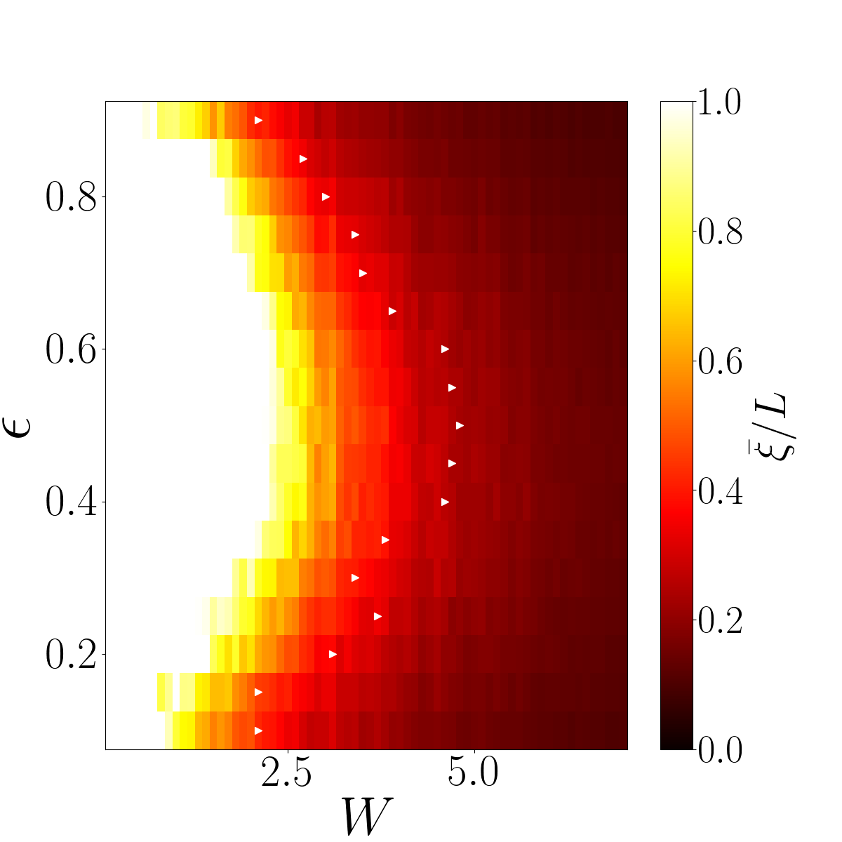
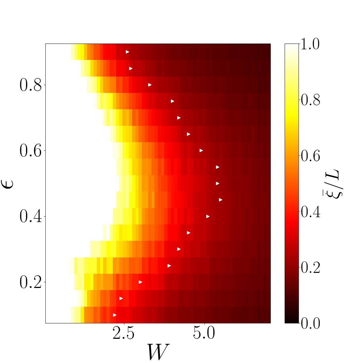
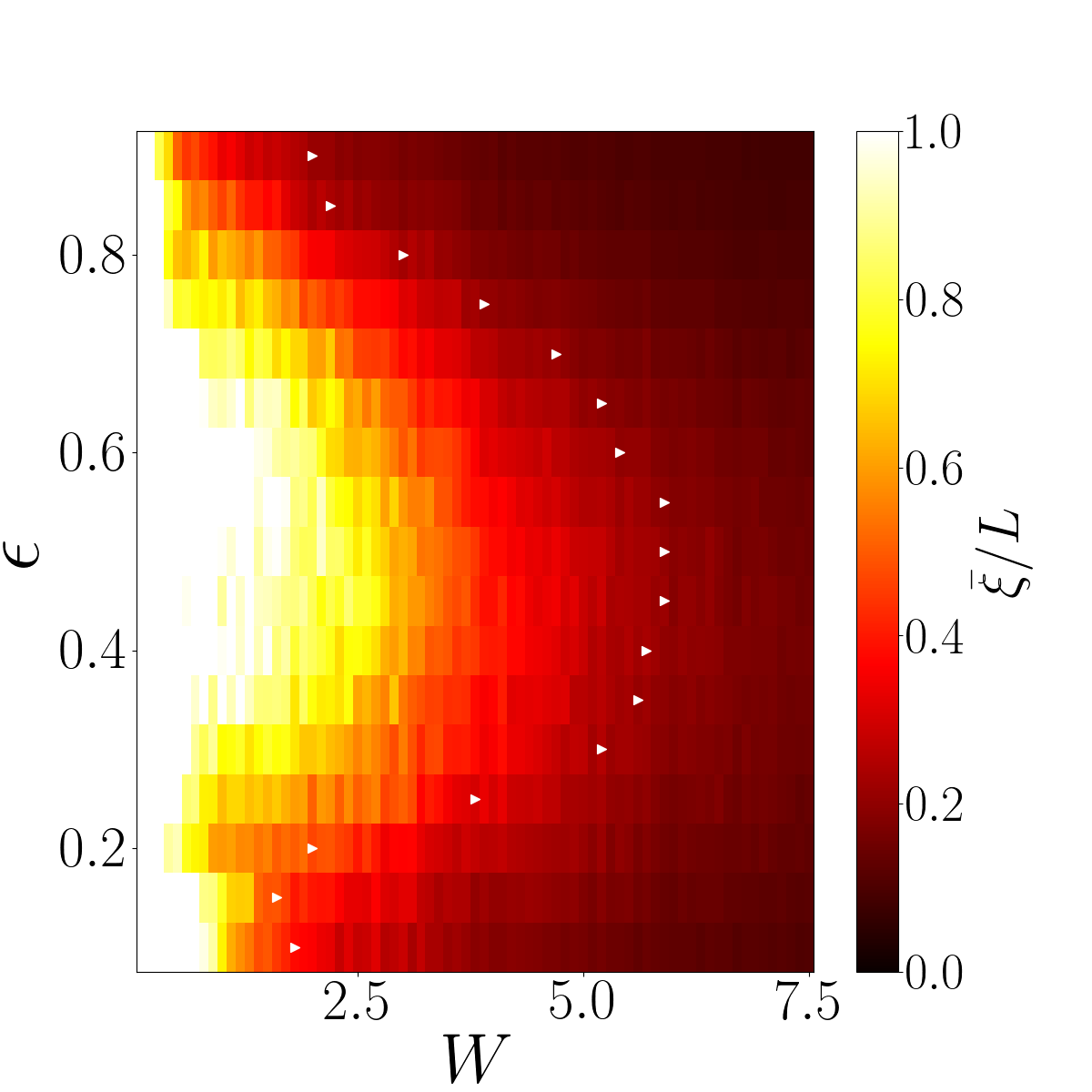
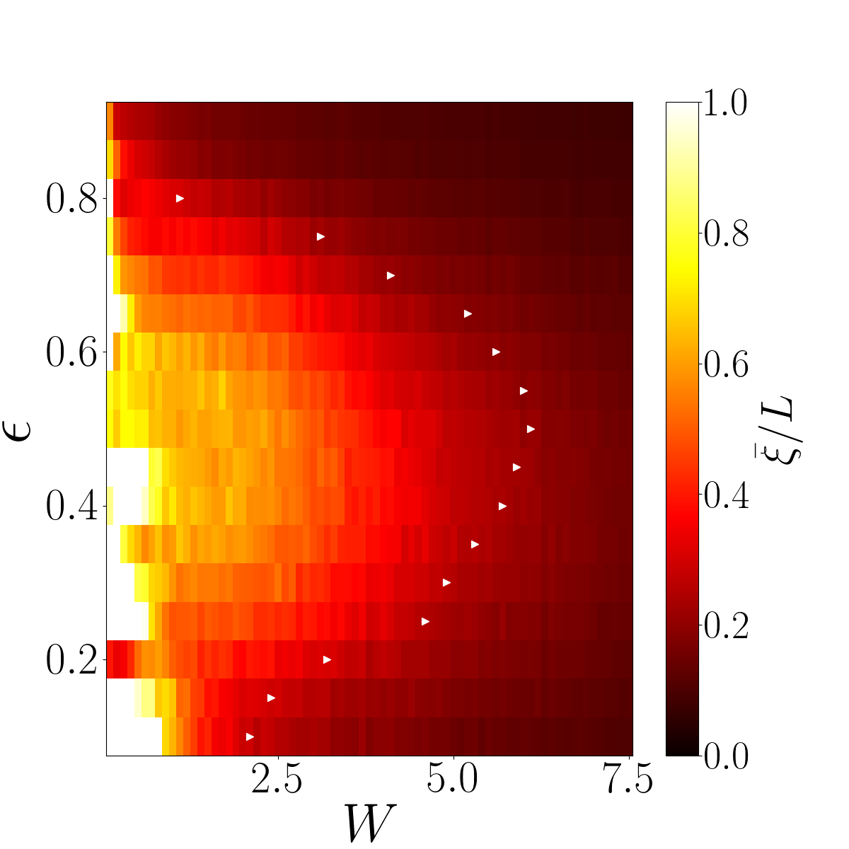
Appendix C Additional Results Regarding Non-Hermitian Avalanches
Here, we show additional numerical results supporting the existence of the non-hermitian avalanche mechanism, as in Fig. 3. Results for a matrix element decay of and are shown in Fig. 14 and Fig. 15, respectively. We see crossovers analogous to those observed in the main text, again occurring roughly at the expected value of .
Appendix D Diagonalizing many-body hamiltonians via generalized displacement transformations
In this appendix, we detail a diagonalization algorithm that iteratively applies a series of transformations eliminating “off-diagonal” terms from a given fermionic Hamiltonian.
Consider fermions hopping on a 1-dimensional lattice with sites . Let , , and be the fermionic annhiliation, creation, and number operators at a site , respectively. A general (hermitian) Hamiltonian then has the form:
| (23) |
where is a diagonal operator, are disjoint subsets of , is a diagonal operator acting only on sites in , and is the operator for hopping between and :
| (24) |
We neglect here the possibility of complex phases multiplying the hopping terms - our algorithm presented below is straightforwardly modified in this case, and the essential results do not change.
Suppose we now want to eliminate the hopping via a unitary change of basis. We can do this by the following transformation
| (25) |
where
| (26) |
and is a diagonal operator acting only on sites in satisfying
| (27) |
where
| (28) |
Application of the transformation (25) to the Hamiltonian (23) results in a Hamiltonian with no terms
of the form present (where is a diagonal operator). Generically, such a Hamiltonian will include new diagonal terms, as well as new hopping terms (created by the action of the transformation on the other hopping terms in (23)).
Now, we can repeatedly apply transformations of the form (25) to eliminate all hopping terms in the original Hamiltonian (23). As mentioned previously, each application of such a transformation generates new hopping terms; in the case of repeated transformations, we can actually re-introduce hoppings that were eliminated by previous transformations. This is not a problem, as the terms that re-introduced will have smaller and smaller “magnitude” over time. To be more precise, let us write out the unitary map in (25) in closed form:
|
|
(29) |
where is the projector onto the subspace in which all sites in either or (but not both) are filled:
|
|
(30) |
In the form (29), we can see that every new hopping term introduced by a transformation of the form (25) will include an operator multiplication by a trigonemtric function of , which will have operator norm . If we iterate such transformations, we can see that the re-introduced hopping terms will converge (in operator norm) to zero. Thus, in the limit of infinitely many transformations of the form (25) applied, all the hopping (non-diagonal) terms will aproach zero, and we will be left with a diagonal Hamiltonian. Numerically, we must cut the procedure off when the largest (given by magnitude of largest matrix element) off-diagonal term has norm below some threshold - we choose this to be .
Note also that by applying the same sequence of transformations to the creation/annhilation operators, we can obtain creation/annhilation operators for the local integrals of motion for the Hamiltonian (23) (assuming it is in the MBL phase). Additionally, if we track the evolution of the hopping terms as we iterate these transformations - or leave certain hopping terms untouched by our transformations - we will see the amplitudes evolve as a function of iteration number. This is reminiscent of a discretized version of the Wegner flow employed by Quito et al. (2016). Indeed, this intuition is how we obtain the “avalanche-like” hopping amplitudes described in the main text.
As a final note, this algorithm can be generalized to non-hermitian Hamiltonians. In such a case, the transformation to eliminate a term of the form
|
|
(31) |
where is diagonal on - is constructed analogously, but now with and in (27) and (29). Note that, if any of the eigenvalues of are negative, and are no longer necessarily bounded in operator norm, and convergence of the algorithm is no longer assured. This is why it is crucial to use the gauge freedom to eliminate the non-hermiticity from the part of the Hamiltonian we are diagonalizing, as described in the main text.
Appendix E Derivation of Cumulative Density Function at the MBL transition
In this appendix, we seek to derive an analytic expression for the distribution of at the MBL transition, based on the (generalized) avalanche condition (16). As it turns out, it is easier to derive the cumulative density function (CDF) of . To that end, let us consider the following more general problem.
Let be a collection of random variables, and a real number. Consider the following extremization problem:
| (32) |
We wish to find the CDF of , given the probability densities of the ’s.
To write down the generic form of this CDF, we first make the following observation:
| (33) |
That is, iff for every value of . Futhermore, we can see that iff . Hence,
| (34) |
The right hand side is the CDF of , evaluated at a point that depends on the other . Using this in the right side of (33), we obtain an expression for in terms of the PDFs of the ’s (i.e., the ’s):
| (35) |
At this point, we can compute the integral over to obtain an integral expression involving the CDF of , but we cannot go any farther without knowledge of the ’s.
To that end, let us now take each of the ’s to be exponentially distributed - that is, for , and for . We can now perform the integrals in (35) for any finite value of , and obtain
| (36) |
This is the desired CDF of , assuming for each . The CDF for a more general exponential distribution can be obtained by making the replacements , .
Let us now connect back to the exceptional points. We have the generalized “avalanche criterion” for :
| (37) |
Comparing (32) with this generalized criterion, and assuming , we see that , with . Assuming at the transition (as observed in Section III.4), it follows that . Therefore, the result (36) with the replacements , and should describe the distribution of at the MBL crossover.
Note that the general formula (35), with appropriate replacements, gives the distribution for whenever an avalanche criterion of the form (37) holds. In particular, if the avalanche criteria holds deep in the MBL regime, this formula should still give the distribution of . Of course, the are not necessarily uniformly distributed away from the crossover region; nonetheless, replacing by the appropriate distribution of should yield the correct distribution for .
Appendix F Additional results from Numerical Fits of Probability distributions
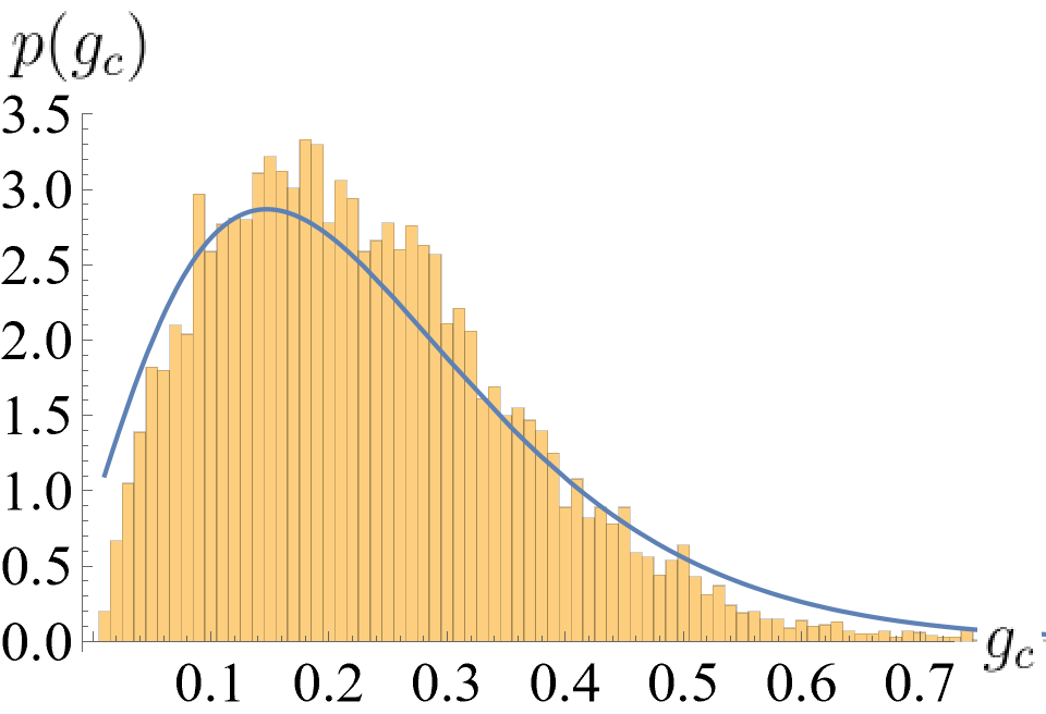
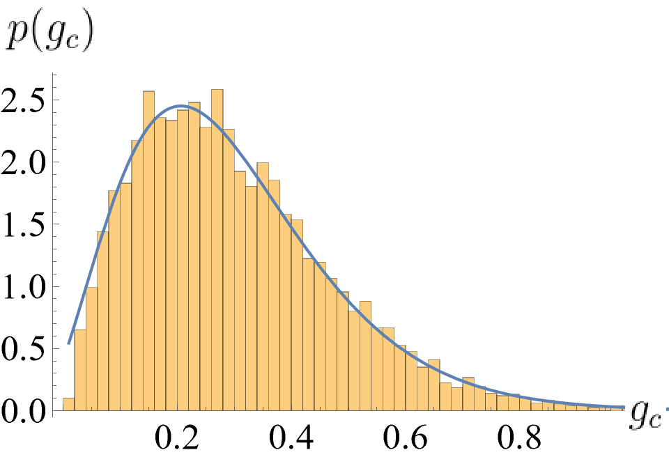
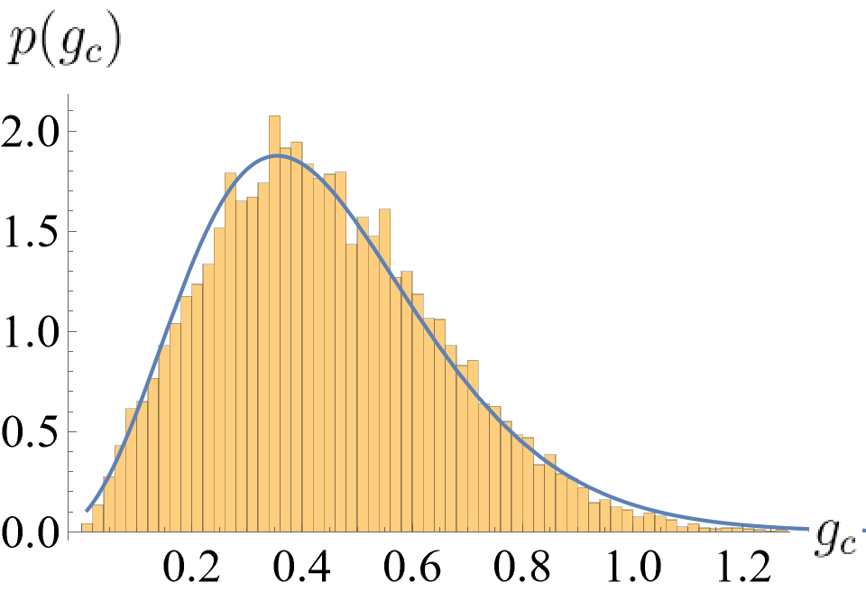
In this appendix, we show some additional results from the numerical fits of the CDFs of described in section IV.
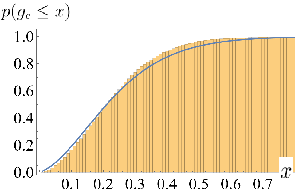
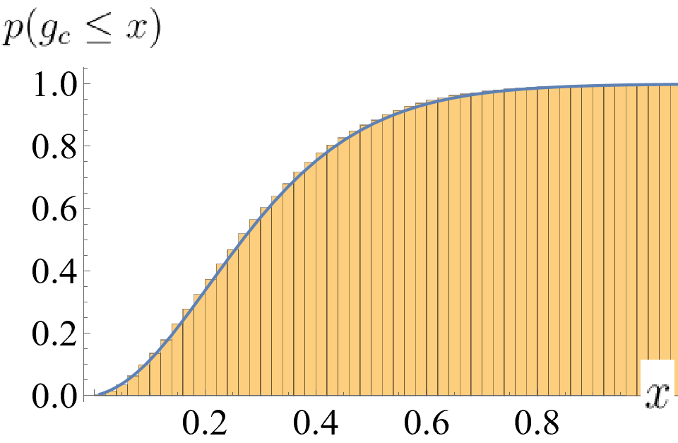
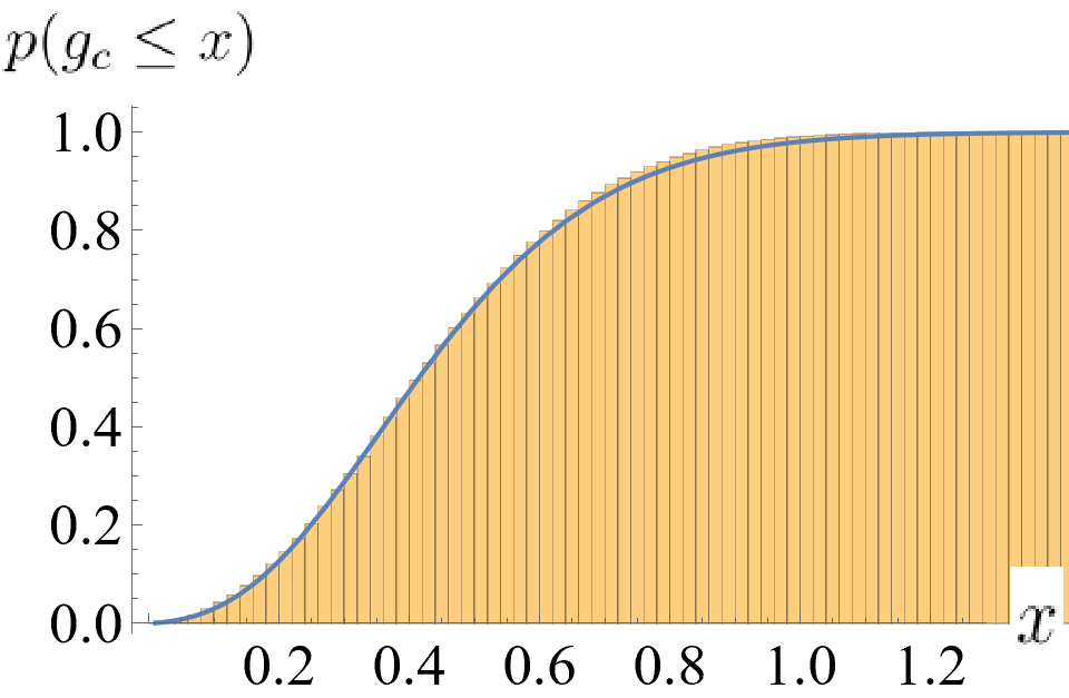
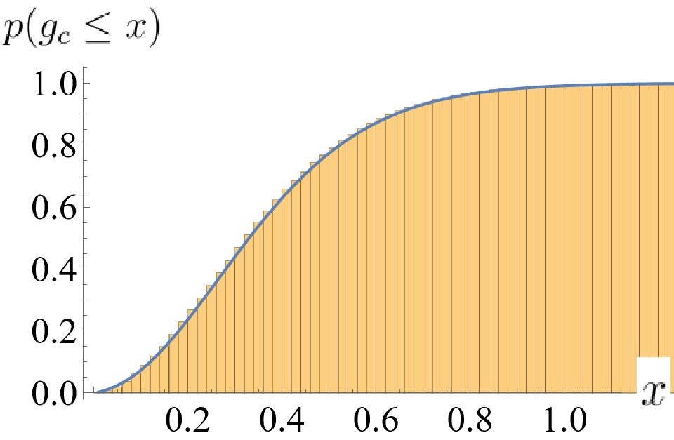
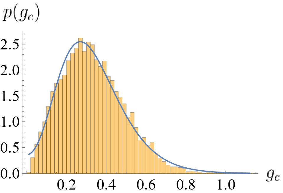
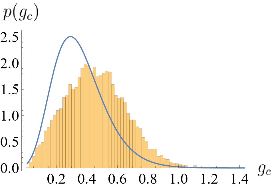
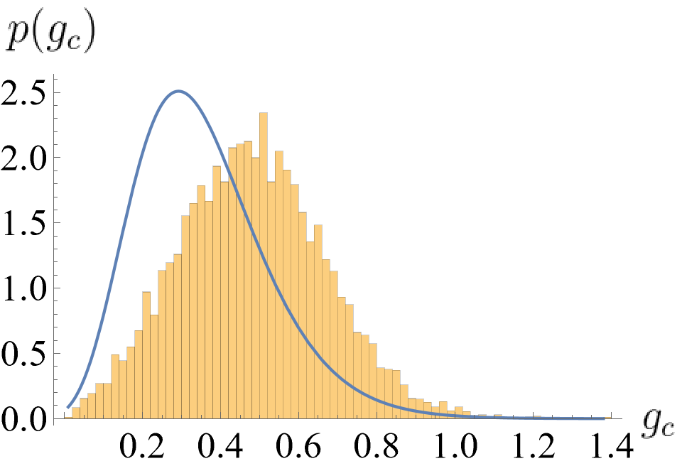
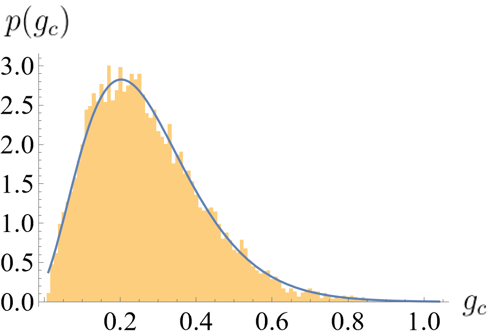
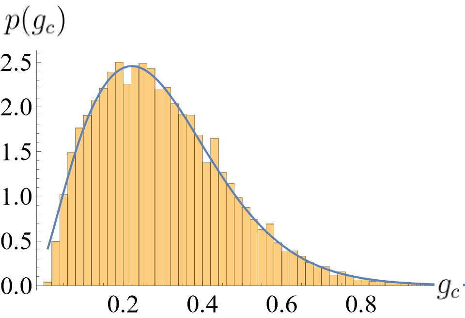
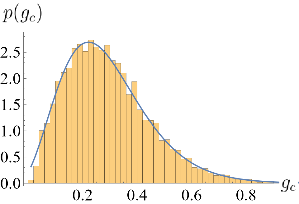
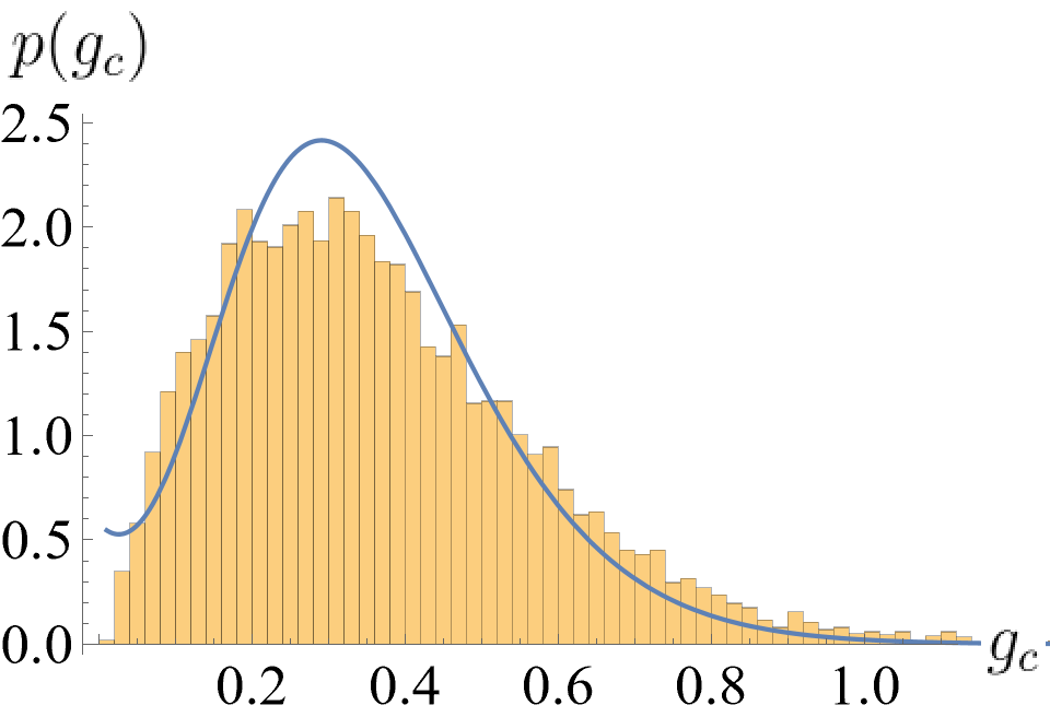
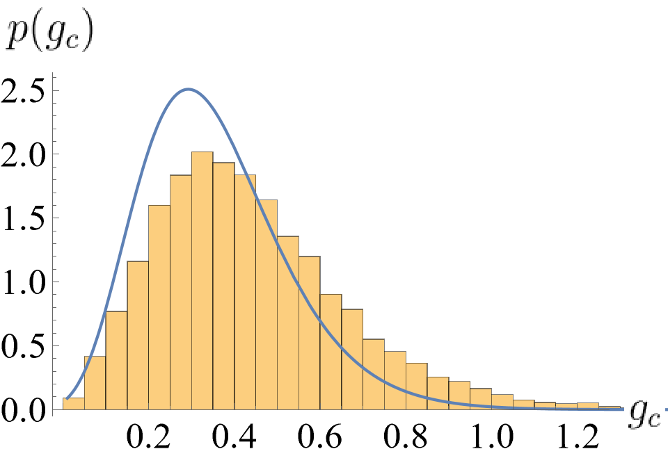
Figure 16 shows the numerically observed probability density function for , along with the analytic PDF obtained by differentiating the best fit mixture distribution of section IV, for the data in Fig 11. We can see that the PDFs generated from our fit have thicker tails (i.e., approach zero more slowly) than the numerically observed PDFs, and that the peak of the numerically observed PDF is larger than the peak of the fitted distribution. Despite these discrepancies, the PDFs from the fits still capture the observed behavior qualitatively well, especially at small and for .
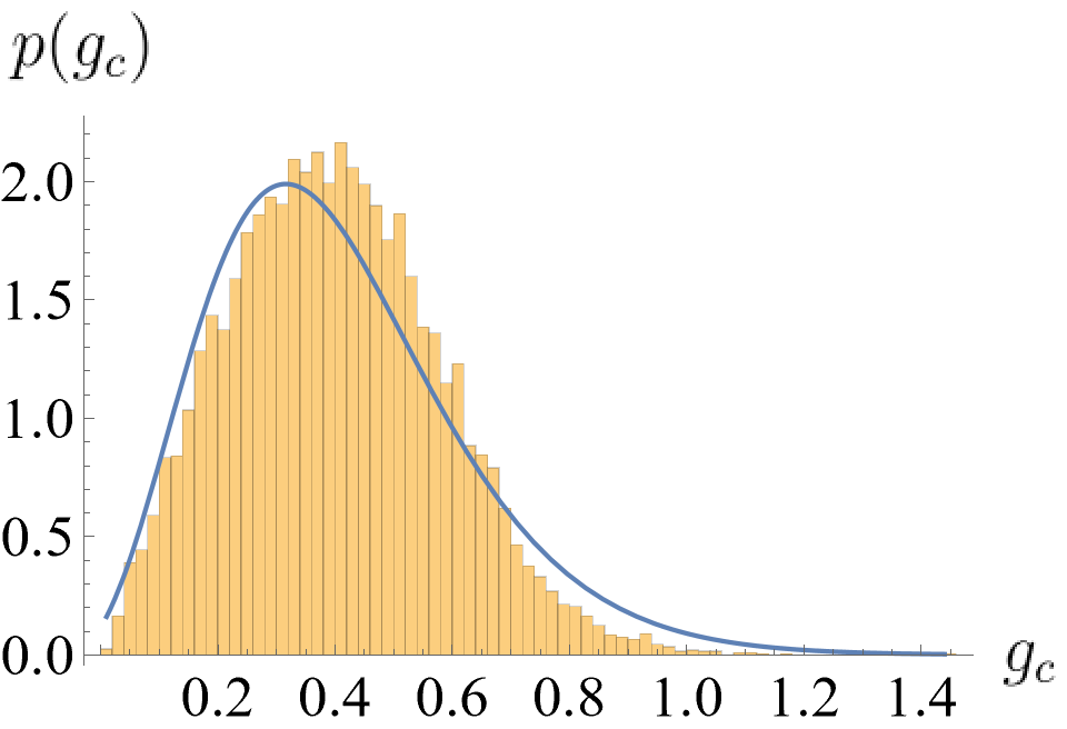
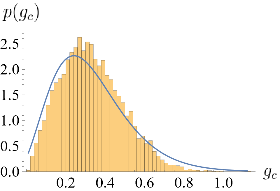
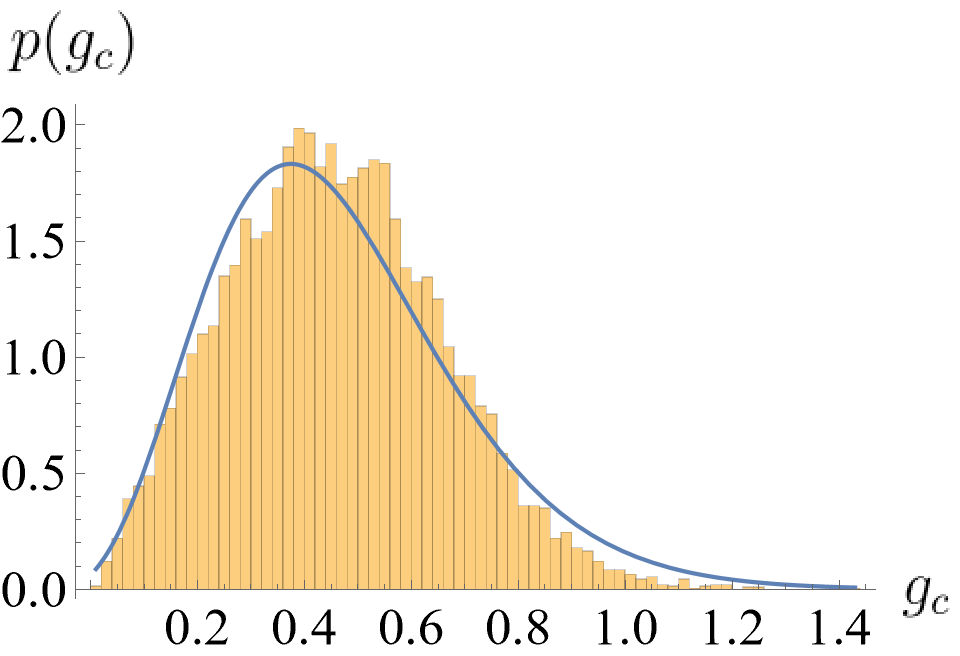
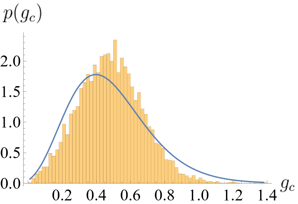
As mentioned in the main text, we observed the numerical fits to be better towards the edges of the spectrum. To exemplify this, Fig. 17 shows the fits for the energy densities whose fitted mixture distribution had the lowest squared error (defined by (19)), and Fig. 18 shows the corresponding PDFs. We see excellent agreement between the observed and fitted distributions, especially for .
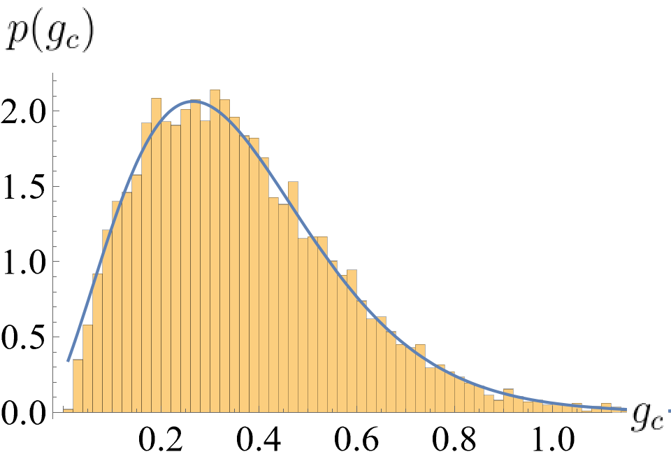
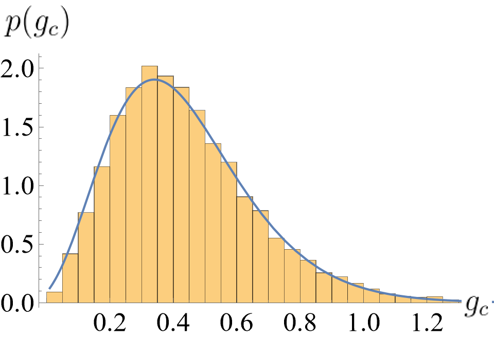
Appendix G Average Avalanche Condition
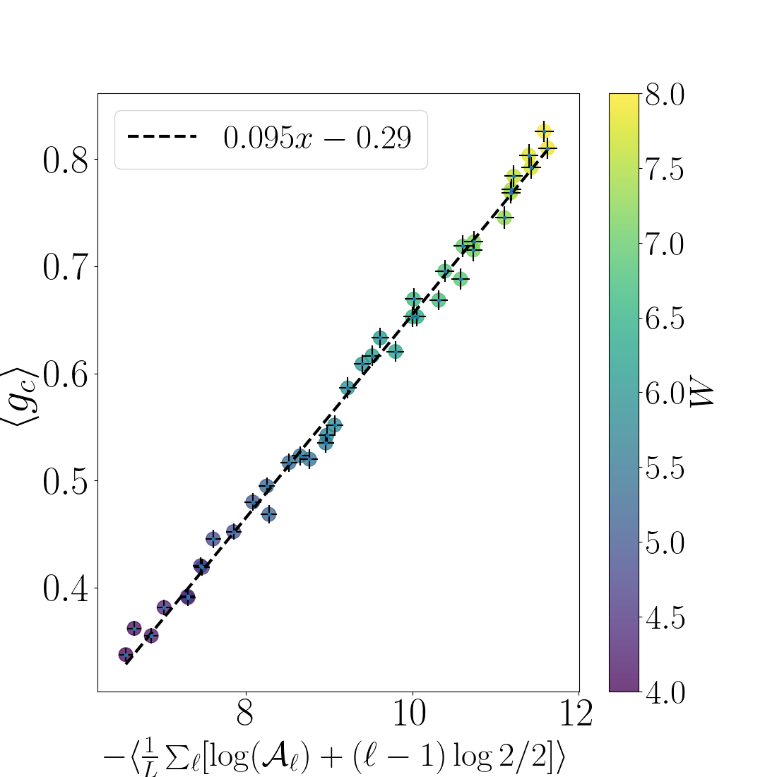
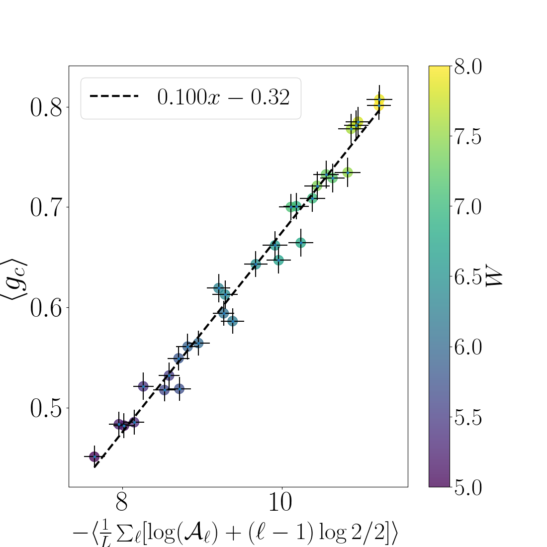
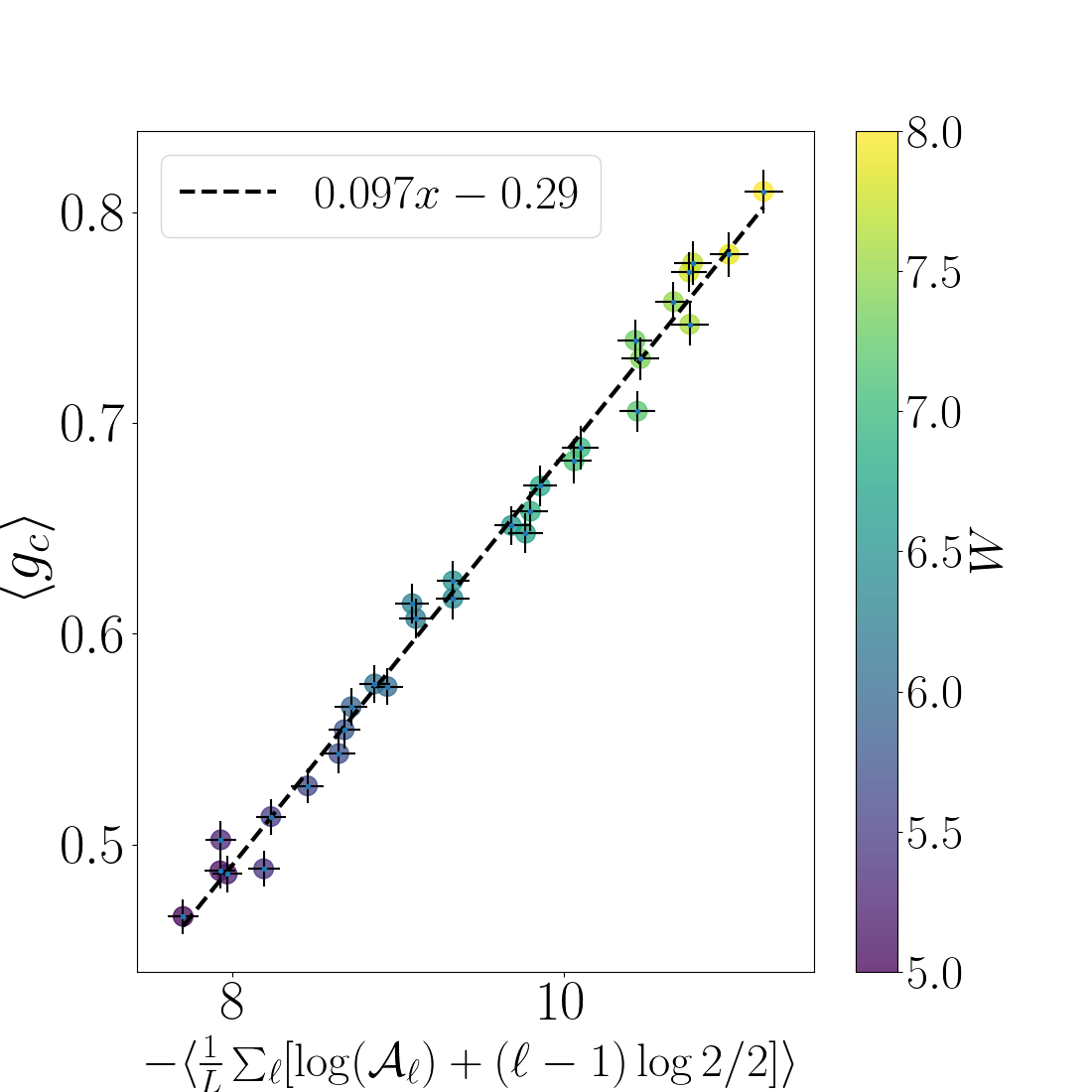
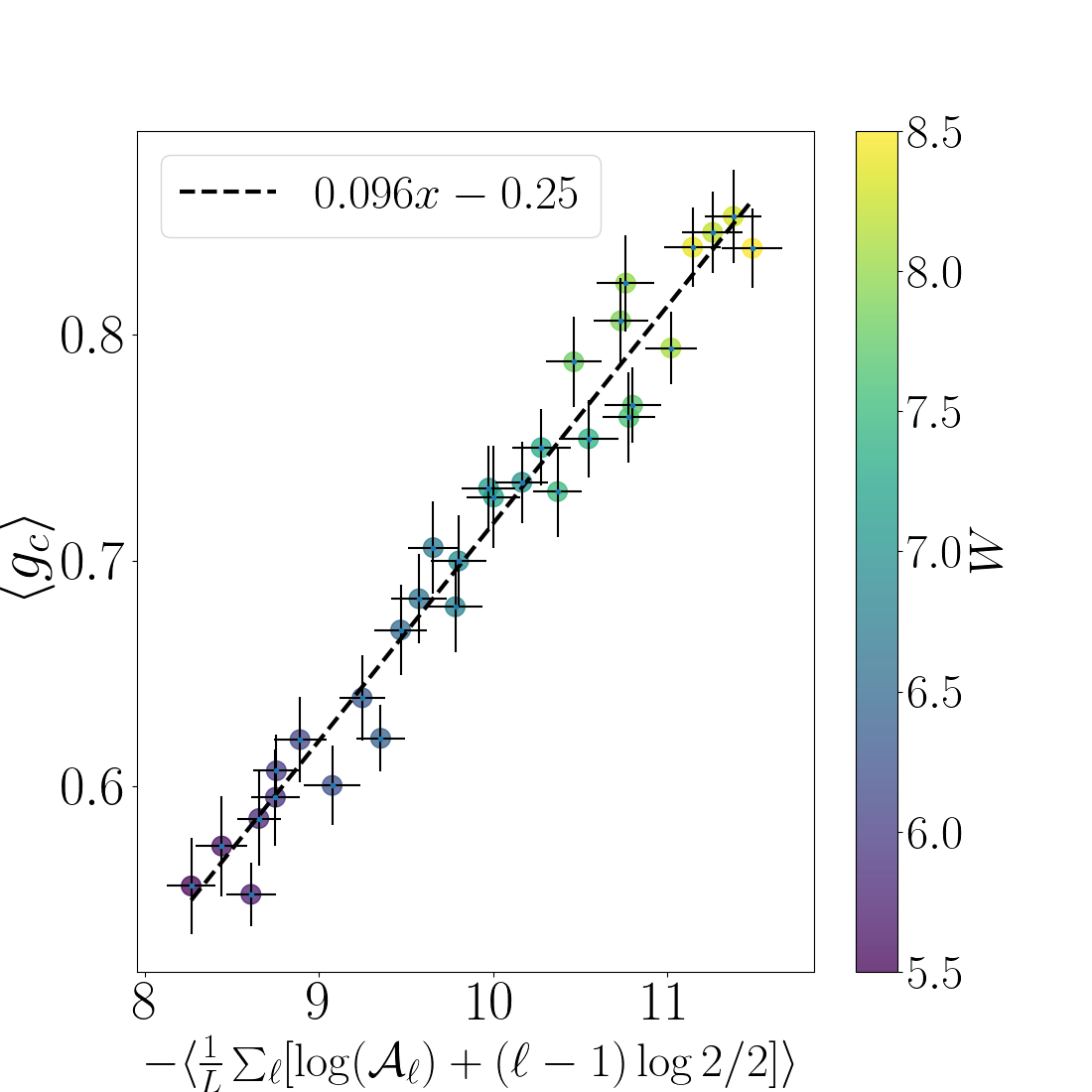
In the process of relating to the amplitudes , we found empirically that was also well-described by a linear relationship with
| (38) |
This quantity is an average over l-bits of the difference between hopping and level spacing, instead of the extremum present in (15). As discussed in Section III.5, such a relationship may be better suited to describing a delocalization mechanism in which the number of l-bits that need to hybridize with the bath for the system to undergo a real-complex transition varies between disorder realizations. Figure 19 shows a scatterplot of versus for individual disorder realizations, akin to Fig. 9. As in Fig. 9, we see a noisy, approximately linear relationship. We perform linear fits of vs , in analogy with Fig. 10; the results of these fits are shown in Fig. 20, and the extracted fit parameters are shown in Table 2. The quality of fit is comparable to those shown in the main text for vs , though the fit parameters are different.
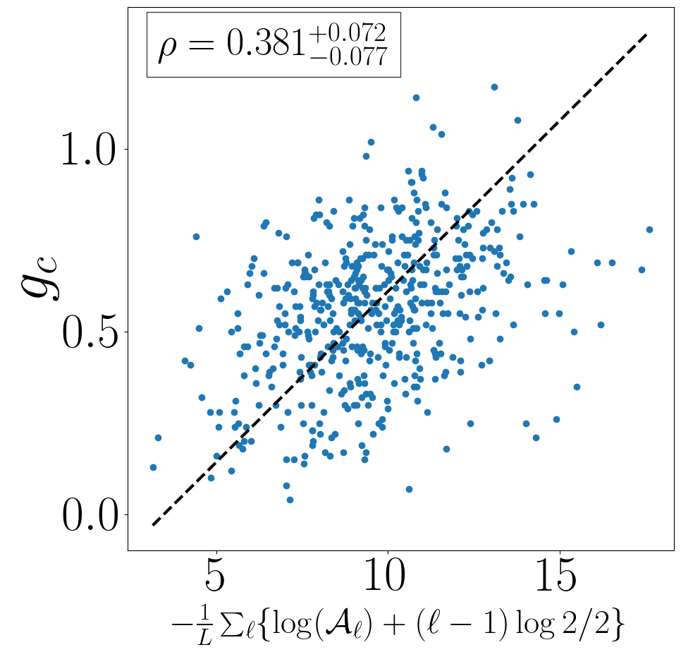
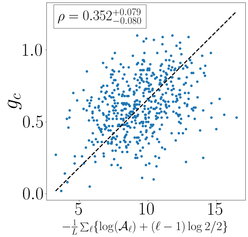
| Slope | Intercept | Slope | Intercept | Slope | Intercept | Slope | Intercept | Slope | Intercept | |
|---|---|---|---|---|---|---|---|---|---|---|
We can derive distributions for at the transition, in analogy with Section IV. To that end, assume that a generalized relation
| (39) |
holds. As before, let us write , so that
Assuming again at the MBL crossover, is exponentially distributed with rate parameter , hence is (up to the shift ) a sum of exponential random variables with rate parameters (). Such a sum is hypoexponentially distributed; the cumulative density for is then Cox (1967)
| (40) |
As before, we construct a mixture distribution of the form (18), and fit the ’s by minimizing the squared error (19). Examples at the center of the spectrum are shown in Fig. 21 and at the band edges in Fig. 22. The resulting probability densities are shown in Figs. 23 and 24. We note that, for lower interaction strengths, we find these fits yield comparable or slightly better (depending on the energy density) squared errors than those of section IV, whereas for stronger interactions the fits described in the main text are clearly superior.
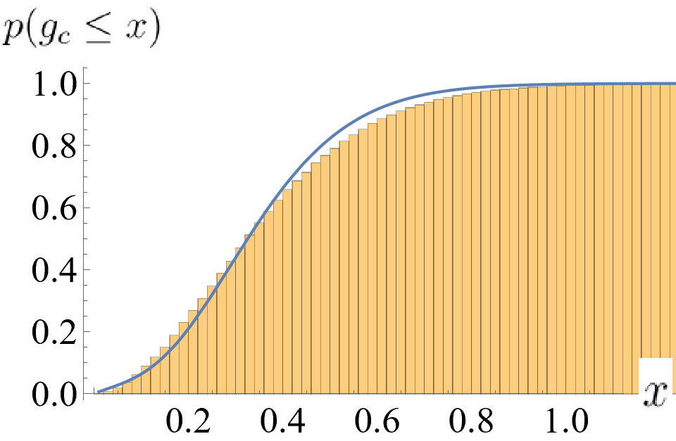
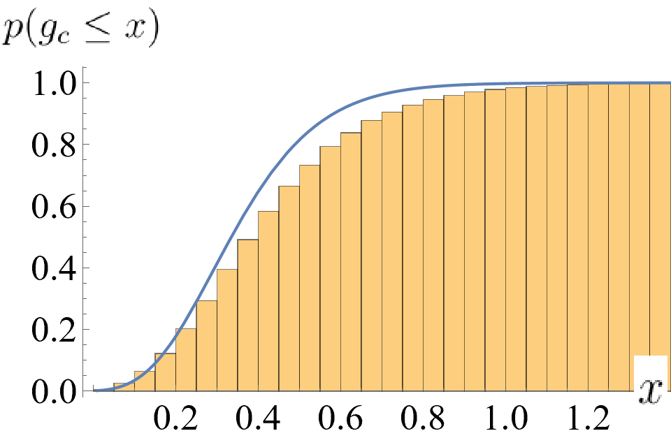
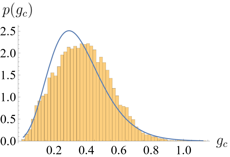
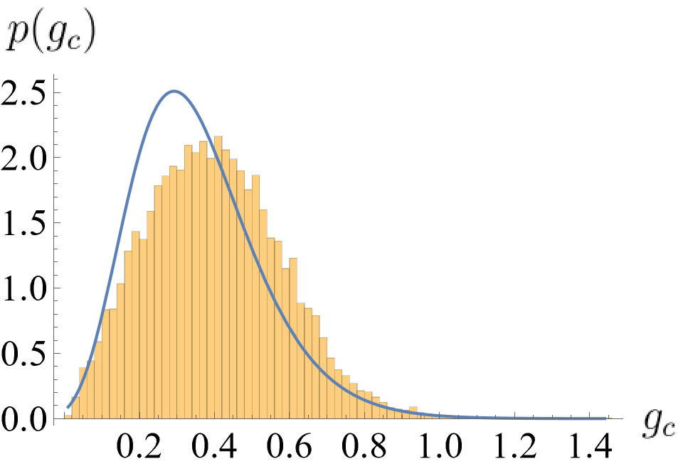
References
- Deutsch (1991) J. M. Deutsch, Phys. Rev. A 43, 2046 (1991), URL https://link.aps.org/doi/10.1103/PhysRevA.43.2046.
- Srednicki (1994) M. Srednicki, Phys. Rev. E 50, 888 (1994), URL https://link.aps.org/doi/10.1103/PhysRevE.50.888.
- Rigol et al. (2008) M. Rigol, V. Dunjko, and M. Olshanii, Nature 452, 854 (2008).
- Rigol and Srednicki (2012) M. Rigol and M. Srednicki, Phys. Rev. Lett. 108, 110601 (2012), URL https://link.aps.org/doi/10.1103/PhysRevLett.108.110601.
- Mori et al. (2018) T. Mori, T. N. Ikeda, E. Kaminishi, and M. Ueda, Journal of Physics B: Atomic, Molecular and Optical Physics 51, 112001 (2018), URL https://doi.org/10.1088/1361-6455/aabcdf.
- Ueda (2020) M. Ueda, Nature Reviews Physics 2, 668 (2020).
- Nandkishore and Huse (2015) R. Nandkishore and D. A. Huse, Annual Review of Condensed Matter Physics 6, 15 (2015), eprint https://doi.org/10.1146/annurev-conmatphys-031214-014726, URL https://doi.org/10.1146/annurev-conmatphys-031214-014726.
- Anderson (1958) P. W. Anderson, Phys. Rev. 109, 1492 (1958), URL https://link.aps.org/doi/10.1103/PhysRev.109.1492.
- Huse et al. (2013) D. A. Huse, R. Nandkishore, V. Oganesyan, A. Pal, and S. L. Sondhi, Phys. Rev. B 88, 014206 (2013), URL https://link.aps.org/doi/10.1103/PhysRevB.88.014206.
- Pekker et al. (2014) D. Pekker, G. Refael, E. Altman, E. Demler, and V. Oganesyan, Phys. Rev. X 4, 011052 (2014), URL https://link.aps.org/doi/10.1103/PhysRevX.4.011052.
- Chandran et al. (2014) A. Chandran, V. Khemani, C. R. Laumann, and S. L. Sondhi, Phys. Rev. B 89, 144201 (2014), URL https://link.aps.org/doi/10.1103/PhysRevB.89.144201.
- Vasseur et al. (2015) R. Vasseur, A. C. Potter, and S. A. Parameswaran, Phys. Rev. Lett. 114, 217201 (2015), URL https://link.aps.org/doi/10.1103/PhysRevLett.114.217201.
- Potter and Vishwanath (2015) A. C. Potter and A. Vishwanath, Protection of topological order by symmetry and many-body localization (2015), URL https://arxiv.org/abs/1506.00592.
- Bahri et al. (2015) Y. Bahri, R. Vosk, E. Altman, and A. Vishwanath, Nat Commun 6 (2015), URL https://www.nature.com/articles/ncomms8341.
- Vasseur et al. (2016) R. Vasseur, A. J. Friedman, S. A. Parameswaran, and A. C. Potter, Phys. Rev. B 93, 134207 (2016), URL https://link.aps.org/doi/10.1103/PhysRevB.93.134207.
- Kells et al. (2018) G. Kells, N. Moran, and D. Meidan, Phys. Rev. B 97, 085425 (2018), URL https://link.aps.org/doi/10.1103/PhysRevB.97.085425.
- Iadecola and Schecter (2018) T. Iadecola and M. Schecter, Phys. Rev. B 98, 144204 (2018), URL https://link.aps.org/doi/10.1103/PhysRevB.98.144204.
- Friedman et al. (2018) A. J. Friedman, R. Vasseur, A. C. Potter, and S. A. Parameswaran, Phys. Rev. B 98, 064203 (2018), URL https://link.aps.org/doi/10.1103/PhysRevB.98.064203.
- Kuno (2019) Y. Kuno, Phys. Rev. Research 1, 032026 (2019), URL https://link.aps.org/doi/10.1103/PhysRevResearch.1.032026.
- Parameswaran and Vasseur (2018) S. A. Parameswaran and R. Vasseur, Reports on Progress in Physics 81, 082501 (2018), URL https://doi.org/10.1088/1361-6633/aac9ed.
- Santos et al. (2005) L. F. Santos, M. I. Dykman, M. Shapiro, and F. M. Izrailev, Phys. Rev. A 71, 012317 (2005), URL https://link.aps.org/doi/10.1103/PhysRevA.71.012317.
- Altshuler et al. (2010) B. Altshuler, H. Krovi, and J. Roland, Proceedings of the National Academy of Sciences 107, 12446 (2010), eprint https://www.pnas.org/doi/pdf/10.1073/pnas.1002116107, URL https://www.pnas.org/doi/abs/10.1073/pnas.1002116107.
- Laumann et al. (2015) C. Laumann, R. Moessner, A. Scardicchio, and S. Sondhi, The European Physcial Journal Special Topics 224, 75 (2015), URL https://link.springer.com/article/10.1140/epjst/e2015-02344-2#citeas.
- Yao et al. (2015) N. Y. Yao, C. R. Laumann, and A. Vishwanath, Many-body localization protected quantum state transfer (2015), URL https://arxiv.org/abs/1508.06995.
- Khemani et al. (2015) V. Khemani, R. Nandkishore, and S. Sondhi, Nat. Phys. 11, 560 (2015), URL https://www.nature.com/articles/nphys3344.
- Goihl et al. (2020) M. Goihl, N. Walk, J. Eisert, and N. Tarantino, Phys. Rev. Research 2, 013120 (2020), URL https://link.aps.org/doi/10.1103/PhysRevResearch.2.013120.
- Pal and Huse (2010) A. Pal and D. A. Huse, Phys. Rev. B 82 (2010), URL https://link.aps.org/doi/10.1103/PhysRevB.82.174411.
- Bauer and Nayak (2013) B. Bauer and C. Nayak, 2013, P09005 (2013), URL https://doi.org/10.1088/1742-5468/2013/09/p09005.
- Žnidarič et al. (2008) M. Žnidarič, T. c. v. Prosen, and P. Prelovšek, Phys. Rev. B 77, 064426 (2008), URL https://link.aps.org/doi/10.1103/PhysRevB.77.064426.
- Kjäll et al. (2014) J. A. Kjäll, J. H. Bardarson, and F. Pollmann, Phys. Rev. Lett. 113, 107204 (2014), URL https://link.aps.org/doi/10.1103/PhysRevLett.113.107204.
- Luitz et al. (2015) D. J. Luitz, N. Laflorencie, and F. Alet, PhysRevB 91 (2015), URL https://link.aps.org/doi/10.1103/PhysRevB.91.081103.
- Imbrie (2016) J. Z. Imbrie, J Stat Phys 163 (2016), URL https://link.springer.com/article/10.1007/s10955-01601508-x.
- Šuntajs et al. (2020) J. Šuntajs, J. Bonča, T. c. v. Prosen, and L. Vidmar, Phys. Rev. E 102, 062144 (2020), URL https://link.aps.org/doi/10.1103/PhysRevE.102.062144.
- Sels and Polkovnikov (2021) D. Sels and A. Polkovnikov, Phys. Rev. E 104, 054105 (2021), URL https://link.aps.org/doi/10.1103/PhysRevE.104.054105.
- Abanin et al. (2021) D. Abanin, J. Bardarson, G. De Tomasi, S. Gopalakrishnan, V. Khemani, S. Parameswaran, F. Pollmann, A. Potter, M. Serbyn, and R. Vasseur, Annals of Physics 427, 168415 (2021), ISSN 0003-4916, URL https://www.sciencedirect.com/science/article/pii/S000349162100021X.
- Gopalakrishnan et al. (2015) S. Gopalakrishnan, M. Müller, V. Khemani, M. Knap, E. Demler, and D. A. Huse, Phys. Rev. B 92, 104202 (2015), URL https://link.aps.org/doi/10.1103/PhysRevB.92.104202.
- Villalonga and Clark (2020a) B. Villalonga and B. K. Clark, Characterizing the many-body localization transition through correlations (2020a), URL https://arxiv.org/abs/2007.06586.
- Villalonga and Clark (2020b) B. Villalonga and B. K. Clark, Eigenstates hybridize on all length scales at the many-body localization transition (2020b), URL https://arxiv.org/abs/2005.13558.
- Garratt et al. (2021) S. J. Garratt, S. Roy, and J. T. Chalker, Phys. Rev. B 104, 184203 (2021), URL https://link.aps.org/doi/10.1103/PhysRevB.104.184203.
- Crowley and Chandran (2022) P. J. D. Crowley and A. Chandran, SciPost Phys. 12, 201 (2022), URL https://scipost.org/10.21468/SciPostPhys.12.6.201.
- Morningstar et al. (2022) A. Morningstar, L. Colmenarez, V. Khemani, D. J. Luitz, and D. A. Huse, Phys. Rev. B 105, 174205 (2022), URL https://link.aps.org/doi/10.1103/PhysRevB.105.174205.
- Long et al. (2022) D. M. Long, P. J. D. Crowley, V. Khemani, and A. Chandran, Phenomenology of the prethermal many-body localized regime (2022), eprint 2207.05761.
- Garratt and Roy (2022) S. J. Garratt and S. Roy, Phys. Rev. B 106, 054309 (2022), URL https://link.aps.org/doi/10.1103/PhysRevB.106.054309.
- Ha et al. (2023) H. Ha, A. Morningstar, and D. A. Huse, Many-body resonances in the avalanche instability of many-body localization (2023), eprint 2301.04658.
- Huse et al. (2014) D. A. Huse, R. Nandkishore, and V. Oganesyan, Phys. Rev. B 90 (2014), URL https://link.aps.org/doi/10.1103/PhysRevB.90.174202.
- Ros et al. (2015) V. Ros, M. Müller, and A. Scardicchio, Nuclear Physics B 891, 420 (2015), ISSN 0550-3213, URL https://www.sciencedirect.com/science/article/pii/S0550321314003836.
- Serbyn et al. (2013) M. Serbyn, Z. Papić, and D. A. Abanin, Phys. Rev. Lett. 111, 127201 (2013), URL https://link.aps.org/doi/10.1103/PhysRevLett.111.127201.
- Chandran et al. (2015) A. Chandran, I. H. Kim, G. Vidal, and D. A. Abanin, Phys. Rev. B 91, 085425 (2015), URL https://link.aps.org/doi/10.1103/PhysRevB.91.085425.
- Rademaker and Ortuño (2016) L. Rademaker and M. Ortuño, Phys. Rev. Lett. 116, 010404 (2016), URL https://link.aps.org/doi/10.1103/PhysRevLett.116.010404.
- Pekker et al. (2017) D. Pekker, B. K. Clark, V. Oganesyan, and G. Refael, Phys. Rev. Lett. 119, 075701 (2017), URL https://link.aps.org/doi/10.1103/PhysRevLett.119.075701.
- Wegner (1994) F. Wegner, Ann. Phys. (Berlin) 506 (1994), URL https://onlinelibrary.wiley.com/doi/10.1002/andp.19945060203.
- Kehrein (2006) S. Kehrein, The Flow Equation Approach to Many-Particle Systems (Springer Berlin, 2006), ISBN 978-3-540-34067-6.
- Peng et al. (2019) P. Peng, Z. Li, H. Yan, K. X. Wei, and P. Cappellaro, Phys. Rev. B 100, 214203 (2019), URL https://link.aps.org/doi/10.1103/PhysRevB.100.214203.
- Kulshreshtha et al. (2018) A. K. Kulshreshtha, A. Pal, T. B. Wahl, and S. H. Simon, Phys. Rev. B 98, 184201 (2018), URL https://link.aps.org/doi/10.1103/PhysRevB.98.184201.
- Varma et al. (2019) V. K. Varma, A. Raj, S. Gopalakrishnan, V. Oganesyan, and D. Pekker, Phys. Rev. B 100, 115136 (2019), URL https://link.aps.org/doi/10.1103/PhysRevB.100.115136.
- Kelly et al. (2020) S. P. Kelly, R. Nandkishore, and J. Marino, Nuclear Physics B 951, 114886 (2020), ISSN 0550-3213, URL https://www.sciencedirect.com/science/article/pii/S0550321319303724.
- Thomson and Schiró (2018) S. J. Thomson and M. Schiró, Phys. Rev. B 97, 060201 (2018), URL https://link.aps.org/doi/10.1103/PhysRevB.97.060201.
- Thomson and Schiró (2020) S. J. Thomson and M. Schiró, Phys. Rev. Res. 2, 043368 (2020), URL https://link.aps.org/doi/10.1103/PhysRevResearch.2.043368.
- Thomson et al. (2021) S. J. Thomson, D. Magano, and M. Schirò, SciPost Phys. 11, 028 (2021), URL https://scipost.org/10.21468/SciPostPhys.11.2.028.
- Thomson and Schirò (2023) S. J. Thomson and M. Schirò, Local integrals of motion in quasiperiodic many-body localized systems (2023), URL https://scipost.org/10.21468/SciPostPhys.14.5.125.
- Quito et al. (2016) V. L. Quito, P. Titum, D. Pekker, and G. Refael, Phys. Rev. B 94, 104202 (2016), URL https://link.aps.org/doi/10.1103/PhysRevB.94.104202.
- Heußen et al. (2021) S. Heußen, C. D. White, and G. Refael, Phys. Rev. B 103, 064201 (2021), URL https://link.aps.org/doi/10.1103/PhysRevB.103.064201.
- De Roeck and Huveneers (2017) W. De Roeck and F. m. c. Huveneers, Phys. Rev. B 95, 155129 (2017), URL https://link.aps.org/doi/10.1103/PhysRevB.95.155129.
- Luitz et al. (2017) D. J. Luitz, F. m. c. Huveneers, and W. De Roeck, Phys. Rev. Lett. 119, 150602 (2017), URL https://link.aps.org/doi/10.1103/PhysRevLett.119.150602.
- Thiery et al. (2018) T. Thiery, F. m. c. Huveneers, M. Müller, and W. De Roeck, Phys. Rev. Lett. 121, 140601 (2018), URL https://link.aps.org/doi/10.1103/PhysRevLett.121.140601.
- Thiery et al. (2017) T. Thiery, M. Müller, and W. D. Roeck (2017), eprint 1711.09880.
- Johri et al. (2015) S. Johri, R. Nandkishore, and R. N. Bhatt, Phys. Rev. Lett. 114, 117401 (2015), URL https://link.aps.org/doi/10.1103/PhysRevLett.114.117401.
- Panda and Banerjee (2020) A. Panda and S. Banerjee, Phys. Rev. B 101, 184201 (2020), URL https://link.aps.org/doi/10.1103/PhysRevB.101.184201.
- Hatano and Nelson (1996) N. Hatano and D. R. Nelson, Phys. Rev. Lett. 77, 570 (1996), URL https://link.aps.org/doi/10.1103/PhysRevLett.77.570.
- Hatano and Nelson (1998) N. Hatano and D. R. Nelson, Phys. Rev. B 58, 8384 (1998), URL https://link.aps.org/doi/10.1103/PhysRevB.58.8384.
- Hatano and Nelson (1997) N. Hatano and D. R. Nelson, Phys. Rev. B 56, 8651 (1997), URL https://link.aps.org/doi/10.1103/PhysRevB.56.8651.
- Kato (1995) T. Kato, Perturbation theory in a finite-dimensional space (Springer Berlin Heidelberg, Berlin, Heidelberg, 1995), pp. 62–126, ISBN 978-3-642-66282-9, URL https://doi.org/10.1007/978-3-642-66282-9_2.
- Heiss and Sannino (1990) W. D. Heiss and A. L. Sannino, Journal of Physics A: Mathematical and General 23, 1167 (1990), URL https://doi.org/10.1088%2F0305-4470%2F23%2F7%2F022.
- Heiss and Sannino (1991) W. D. Heiss and A. L. Sannino, Phys. Rev. A 43, 4159 (1991), URL https://link.aps.org/doi/10.1103/PhysRevA.43.4159.
- Heiss (2000) W. D. Heiss, Phys. Rev. E 61, 929 (2000), URL https://link.aps.org/doi/10.1103/PhysRevE.61.929.
- Heiss (2001) W. D. Heiss, AIP Conference Proceedings 597, 311 (2001), eprint https://aip.scitation.org/doi/pdf/10.1063/1.1427477, URL https://aip.scitation.org/doi/abs/10.1063/1.1427477.
- Heiss and Harney (2001) W. D. Heiss and H. Harney, Eur. Phys. J. D 17, 149 (2001), URL https://link.springer.com/article/10.1007/s100530170017.
- Heiss (2004) W. D. Heiss, Journal of Physics A: Mathematical and General 37, 2455 (2004), URL https://doi.org/10.1088/0305-4470/37/6/034.
- Heiss (2008) W. D. Heiss, Journal of Physics A: Mathematical and Theoretical 41, 244010 (2008), URL https://doi.org/10.1088/1751-8113/41/24/244010.
- Heiss (2012) W. D. Heiss, Journal of Physics A: Mathematical and Theoretical 45, 444016 (2012), URL https://doi.org/10.1088/1751-8113/45/44/444016.
- Luitz and Piazza (2019) D. J. Luitz and F. Piazza, Phys. Rev. Research 1, 033051 (2019), URL https://link.aps.org/doi/10.1103/PhysRevResearch.1.033051.
- Hamazaki et al. (2019) R. Hamazaki, K. Kawabata, and M. Ueda, Phys. Rev. Lett. 123, 090603 (2019), URL https://link.aps.org/doi/10.1103/PhysRevLett.123.090603.
- Feinberg and Zee (1999a) J. Feinberg and A. Zee, Phys. Rev. E 59, 6433 (1999a), URL https://link.aps.org/doi/10.1103/PhysRevE.59.6433.
- Feinberg and Zee (1999b) J. Feinberg and A. Zee, Nuclear Physics B 552, 599 (1999b), ISSN 0550-3213, URL https://www.sciencedirect.com/science/article/pii/S0550321399002461.
- Brézin and Zee (1998) E. Brézin and A. Zee, Nuclear Physics B 509, 599 (1998), ISSN 0550-3213, URL https://www.sciencedirect.com/science/article/pii/S0550321397006524.
- Potirniche et al. (2019) I.-D. Potirniche, S. Banerjee, and E. Altman, Phys. Rev. B 99, 205149 (2019), URL https://link.aps.org/doi/10.1103/PhysRevB.99.205149.
- Burnham and Anderson (2004) K. P. Burnham and D. R. Anderson, Sociological Methods & Research 33, 261 (2004), eprint https://doi.org/10.1177/0049124104268644, URL https://doi.org/10.1177/0049124104268644.
- Rodriguez et al. (2011) A. Rodriguez, L. J. Vasquez, K. Slevin, and R. A. Römer, Phys. Rev. B 84, 134209 (2011), URL https://link.aps.org/doi/10.1103/PhysRevB.84.134209.
- Cox (1967) D. R. Cox, Renewal theory., Methuen’s monographs on applied probability and statistics (Methuen; [distributed in the USA by Barnes & Noble, 1967), URL https://search.ebscohost.com/login.aspx?direct=true&AuthType=ip,sso&db=cat09073a&AN=cit.oai.edge.caltech.folio.ebsco.com.fs00001057.62fa39eb.c0bc.4443.8272.a7be9a56a9fe&site=eds-live&scope=site.