Phase classification in the long-range Harper model using machine learning
Abstract
In this work, we map the phase diagrams of one-dimensional quasiperiodic models using artificial neural networks. We observe that the multi-class classifier precisely distinguishes the various phases, namely the delocalized, multifractal, and localized phases, when trained on the eigenstates of the long-range Aubry-André Harper (LRH) model. Additionally, when this trained multi-layer perceptron is fed with the eigenstates of the Aubry-André Harper (AAH) model, it identifies various phases with reasonable accuracy. We examine the resulting phase diagrams produced using a single disorder realization and demonstrate that they are consistent with those obtained from the conventional method of fractal dimension analysis. Interestingly, when the neural network is trained using the eigenstates of the AAH model, the resulting phase diagrams for the LRH model are less exemplary than those previously obtained. Further, we study binary classification by training the neural network on the probability density corresponding to the delocalized and localized eigenstates of the AAH model. We are able to pinpoint the critical transition point by examining the metric “accuracy” for the central eigenstate. The effectiveness of the binary classifier in identifying a previously unknown multifractal phase is then evaluated by applying it to the LRH model.
I INTRODUCTION
The application of machine learning (ML) techniques in the field of condensed matter physics has been a subject of great interest in recent times [1]. This interdisciplinary field has rapidly gained popularity owing to the advantages presented by machine learning [2, 3, 4]. As an actively evolving area of research, ML techniques have been used to detect classical and quantum phase transitions [5, 6, 7, 8, 9, 10, 11, 12, 13], for the acceleration of Monte Carlo simulations [14, 15, 16], and for representation of states of quantum many-body systems [17, 18, 19, 20, 21, 22, 23, 24, 25, 22, 26]. A popular subcategory of machine learning is supervised learning [27], where one trains algorithms to utilize labelled training datasets in order to classify new data or make predictions accurately. This motivates its application in condensed matter physics for classifying various phases in strongly correlated systems [5, 28], topological systems [29, 30, 31] and quantum many-body systems [17, 9].
Disordered quantum systems [32, 33, 34, 35, 36, 37] have been a fascinating topic of study for a long time. In the 1-D Anderson model [32], the tiniest of disorder is known to localize single-particle states exponentially. In contrast, the Aubry-Andrè-Harper (AAH) [38, 39] model, governed by a quasiperiodic disorder, exhibits a delocalization-localization transition even in one dimension. Interestingly, instead of the exponential localization observed in the short-ranged model, the eigenstates show algebraic localization [40, 41, 42] in the case of long-range hopping. This has naturally led to exciting studies exploring the effects of quasiperiodic disorder in long-range systems [43, 44].
The interplay of power law hopping and the quasiperiodic potential results in a rich structure [43] in the single particle eigenstates. The self-duality of the quasiperiodic AAH model is broken, and mobility edges are observed when the hopping is no longer restricted to nearest neighbours only. While multifractal eigenstates are observed to coexist with delocalized eigenstates for , localized states exist together with delocalized eigenstates for [43]. The localization characteristics of these single particle eigenstates have been determined [43, 45] with the aid of several well-known measures, such as fractal dimension [46, 47], inverse participation ratio [48, 49], level spacing [50] and many more. These methods depend on a physical understanding of the nature of the regime.
In the present work, we construct a neural network for characterizing the phase diagram beyond established methods in single-particle Hamiltonian models. We study the one-dimensional long-range AAH (LRH) model, where multifractal (localized) eigenstates can coexist with delocalized eigenstates for the long-range hopping parameter . The information required for classifying the delocalized, localized and multifractal regimes is obtained from the eigenstates which are used as inputs to the neural network. The trained network is first used to classify all the eigenstates of the LRH model for various values of the hopping parameter . We then consider the case of , i.e., the standard AAH model and classify its eigenstates as delocalized/localized/multifractal. We show that the phase diagram obtained by feeding a single disorder realization in the neural network is in good agreement with results obtained using conventional methods. We next train the same network using the eigenstates of the AAH model. In this case, although the network can identify the localized phase accurately, some discrepancy is seen in the case of multifractal and delocalized states. We also utilize binary classification to identify the transition point of the AAH model by training the neural network on its delocalized and localized eigenstates. While this network precisely identifies the phase diagram for the AAH model, it can also identify the multifractal phase (for which no explicit training is given) of the LRH model, although this is achieved only in a coarse manner.
This paper is organized as follows. Section II discusses the details of the Hamiltonian model and carries an introduction to the general setup of the neural network. In Section III, we discuss the network architecture used for the classification as well as the details of the input data. In Section IV, we present our multi-class and binary classification results and compare them against the results obtained through a conventional method. We then summarize our results in Section V. The utilization of the binary classifier trained on the data of a 1-D model, to predict the phase diagram of a D model is discussed in the Appendix.
II Model and Methods
II.1 Hamiltonian
We consider the one-dimensional long-range Harper (LRH) model given by the Hamiltonian:
| (1) |
where represents the single particle creation (destruction) operator at site . The first term describes hopping, where is the geometric distance between the sites and in a ring. The strength of the long-range hopping is controlled by , which we set to unity and the long-range parameter in the hopping, namely . The second term describes the quasiperiodic on-site energy, where the strength of the quasiperiodic potential is , and the quasiperiodicity parameter is taken to be an irrational number, set as the golden mean [51]. is an arbitrary global phase chosen randomly from a uniform distribution in the range. The total number of sites is , and periodic boundary conditions are assumed. In the limit , the hopping is effectively nearest-neighbour, and we recover the standard AAH model: [38, 39]
| (2) |
It is well known [51] that all the energy eigenstates are delocalized when , and all the energy eigenstates are localized when . is the critical point where all the eigenstates are multifractal [52]. It is known that the AAH model is self-dual [38, 53]; at the critical point , the AAH model in position space maps to itself in momentum space. When long-range hopping is introduced ( is finite), the self-duality condition is broken.
II.2 Artificial neural network
The artificial neural network (ANN) is inspired by the neuronal network in the biological brain [54, 55]. The ANN combines a series of linear maps and non-linear functions [56] that are successively applied to the input data in order to obtain the final output. A mapping defines each layer of the network, and the dimension of a layer corresponds to the number of neurons in it. In this work, in the case of multi-class classification, we utilize vectors of dimension and train a map to map them to the target set . One-hot vectors represent this target set and deliver the final output in the form of entries of the neurons of the output layer. The network is trained on a data set called the training set, and its performance is gradually improved by adjusting its parameters. In supervised learning, the training set consists of labelled data, i.e., for each input , the output is already known to map to one of the outcomes of the target set. The trained network then classifies previously unseen data from the testing set.
We next describe the functioning of the neural network. The ‘input layer’ maps the initial vectors of dimension to a space of dimension with the help of a linear map and a non-linear activation function [57]. Subsequently, the mapping between the and the layer is defined as:
| (3) |
Here matrix-vector multiplication is implied between (matrix of dimension ) and (vector of dimension ). The resulting vector is a vector of dimension . The elements of the matrix are called the weights, and the corresponding elements of the vector are called the biases. The final layer of the ANN is referred to as the ‘output layer’, with the number of nodes equal to the number of expected outputs that the network is trained for. The layers between the input and output layers are called hidden layers, which can range from one to several. The method of training neural networks with multiple hidden layers is referred to as deep learning [58]. Also, if the number of neurons in a layer is huge, the network learns non-universal features and unnecessary details for classification. This can lead to overfitting of data. Thus in this study we employ dropout regularisation [59] to avoid the gradual accumulation of neuronal weight configurations.
In the case of multi-class classification, the inputs to the network consist of the amplitudes of an eigenstate of the Hamiltonian of interest. For the hidden layers, we utilize the Leaky Rectified Linear Unit (ReLU) activation function [60] defined as:
| (4) |
In the output layer, we consider the Softmax activation function [61] defined as:
| (5) |
The Softmax function estimates the output corresponding to each target set vector, which sums up to unity. These projections can be interpreted as the confidence of the network to assign a class to the input data.
In the case of binary classification, since the probability densities are considered as inputs, we utilize the ReLU activation function [62]:
| (6) |
in the hidden layers. In the output layer, we employ the Sigmoid activation function [61] defined as:
| (7) |
to obtain a single output. There are two main advantages of the ReLU function: (a) it is computationally efficient as it only involves a simple comparison and (b) it introduces non-linearity in the model. On the other hand, the Sigmoid function has a smooth and continuous output, which makes it easier to compute gradients during backpropagation and to optimize the model using gradient-based methods such as the stochastic gradient descent. The activation functions in the hidden and output layers of both the neural networks are compiled in Table 1.
| Neural Network | Hidden layer activation function | Output layer activation function |
|---|---|---|
| Multi-class classifier | Leaky ReLU | Softmax |
| Binary classifier | ReLU | Sigmoid |
In order to correctly estimate various parameters such as the weights and biases, the network utilizes a loss/cost function [63] as well as an optimizer during the training process. The cost function measures the distance between the predicted outputs and their actual values. In general, cross-entropy is widely used as a loss function when optimizing classification models. For classification problems, we utilize the cross-entropy loss function:
| (8) |
where denotes the number of classes, are the probabilities obtained from the Softmax/Sigmoid output layer, and are the true values namely or .
Another step involved in network training is back-propagation [64], where the weights and biases are adjusted in successive iterations to reduce the output of the loss function. The updating rate of the parameters is called the learning rate. This is done through the gradient descent optimization algorithm, which is computationally expensive. To overcome storage issues, the training data is broken down into small batches, which can be easily fed to the model. When the entire training data is fed to the model in batches, it is called an epoch. Thus, every batch in the training data set can update the internal model parameters once during an epoch. In order for the model to learn the gradient or the direction it should take to minimize the loss function, we employ an adaptive learning rate optimizer Adam [65] which incorporates adaptive estimates of the gradients and their squares. The neural network evaluates the loss function on the training dataset at the end of each epoch - this is known as the training loss [66]. An additional data set for validation is considered for every epoch to determine whether or not the network is fully trained, that is, if it can generalize its knowledge to sets of previously unseen data. The neural network is then made to evaluate the loss function on the validation dataset - this is known as the validation loss. The training and validation loss for a good fit should gradually reduce and converge to as the number of epochs increases.
III Neural network approach
We perform exact diagonalization on the Hamiltonian to obtain the single-particle eigenstates. Our goal is to be able to build an effective neural network that can classify these eigenstates according to their localization properties. We build and analyze two neural networks: a multi-class and a binary classification network. While the amplitudes of the eigenstates are utilized as inputs for the multi-class classification network, the on-site probability densities drawn from the eigenstates are taken to be the inputs in the case of the binary classification network. We discuss both cases in detail below.
III.1 Multi-class classification
We consider a system with sites, and obtain the single-particle eigenstates of the LRH model [45] given by Eq. 1. We then generate the training data by varying the disorder strength in small steps () in the range of for the long-range hopping parameter strengths and for several disorder samples. As mentioned earlier, the multifractal (localized) eigenstates coexist with delocalized eigenstates for in the LRH model; the chosen parameters help us to obtain data corresponding to all the three classes, i.e., delocalized, multifractal and localized.
(a)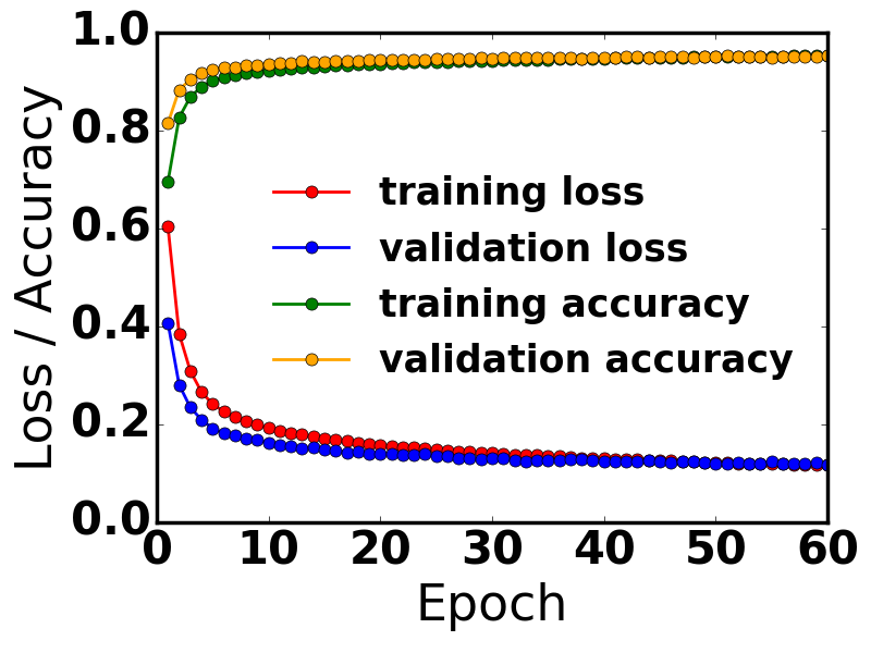 \stackunder(b)
In order to label the eigenstates required for network training, we calculate a well-known quantity called fractal dimension [52, 67, 68] by coarse-graining the system into boxes of length . Given a normalized wave function defined over a lattice of size , we divide the lattice into segments of length [69]. The fractal dimension is then defined as:
| (9) |
The fractal dimension in the limit is given by [52]:
| (10) |
For a perfectly delocalized state, while for a localized state, is vanishing, for all . For intermediate cases, , which is a sign that the state is multifractal.
Here for each eigenstate, we calculate the fractal dimension and label it as follows:
| Localized, | ||||
| Multifractal, | ||||
| (11) |
(a)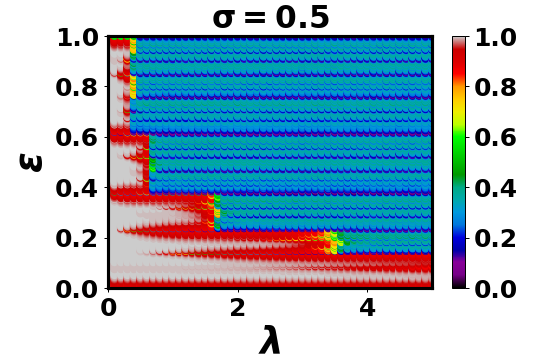 \stackunder(b)
 \stackunder(c)
(d)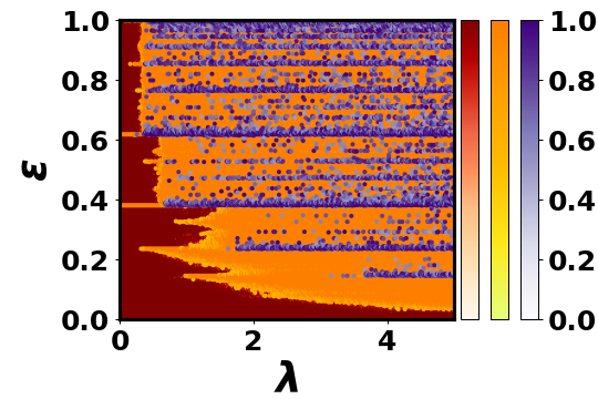 \stackunder(e)
 \stackunder(f)
(g)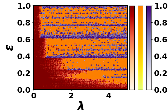 \stackunder(h)
 \stackunder(i)
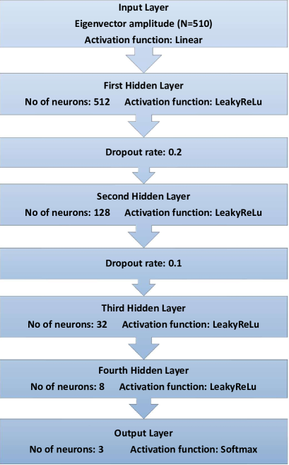
We first generate a training data set comprising of eigenstates of the LRH model belonging to each of the three classes, by considering various values of , , and . A schematic flowchart to describe the complete architecture of the neural network performing multi-class classification is shown in Fig. 1. The network comprises of an input layer, several hidden layers and an output layer coupled to Linear, Leaky ReLU and Softmax activation functions, respectively. We have also added dropout layers to the model to avoid overfitting. The cost function is cross-entropy, and the neural network weights are optimized using the Adam optimizer. We consider batch sizes of samples, which add up to samples per epoch, with an split between training and validation. We observe that fixing the number of training epochs to allows us to obtain an accuracy of as shown in Fig. 2(a). Here accuracy is defined as the ratio of eigenstates correctly classified to the total number of eigenstates. Once the network is trained, the eigenvectors from each point in the phase space of are fed to the network. We obtain three values each of which lies between and and correspond to the neural network’s confidence of classifying the given input in each phase/class.
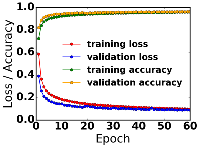
We next generate another training data set comprising of eigenstates of the AAH model given by Eq. 2. Once again the training set consists of eigenstates belonging to each class classified as localized, multifractal and delocalized using (see Eq. 11). The network architecture is the same as before (see Fig. 1). The neural network weights are tuned using an Adam optimizer, and the cost function is cross-entropy as before. Here again training epochs have been considered, and the batch size is . The split between training and validation is followed once again. As demonstrated in Fig. 2(b), the network is trained to an accuracy of .
(a)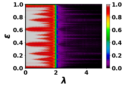 \stackunder(b)
 \stackunder(c)
III.2 Binary classification
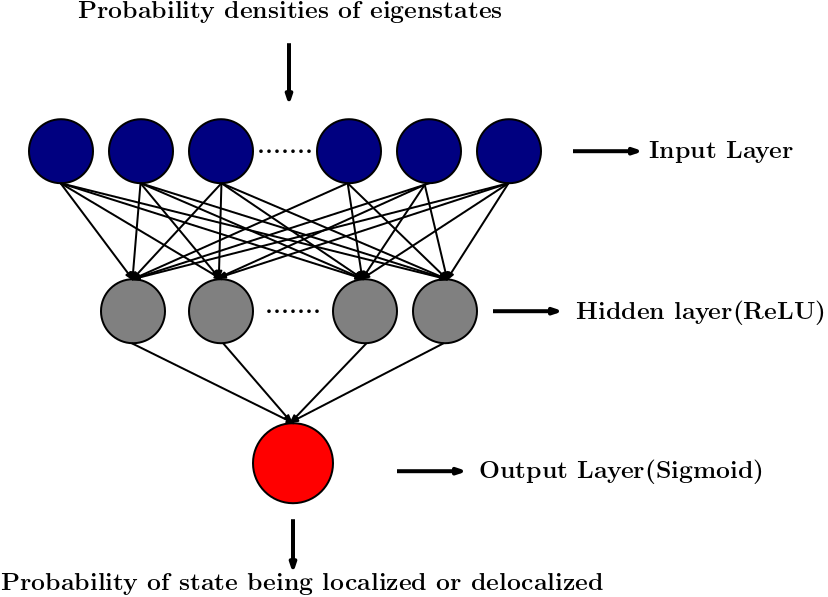
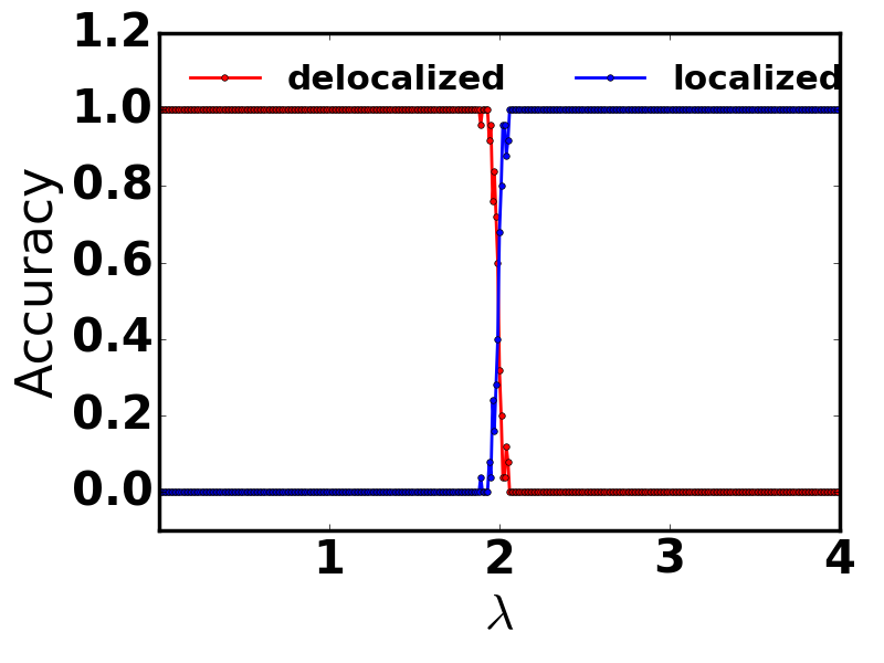
For binary classification, we train the network using the on-site probability densities (PDs) of the delocalized and localized eigenstates of the AAH model. As mentioned earlier, all the eigenstates are delocalized (localized) below (above) a critical disorder strength , at which the eigenstates show multifractal behaviour. For a system size of , we consider disorder realizations () generating samples separately for the delocalized and localized classes by choosing disorder strengths and , respectively. We construct a neural network which consists of an input layer of size and utilizes on-site probability densities of the eigenstates as inputs. This is followed by a single hidden layer with the number of neurons equal to the greatest integer less than . The neurons are coupled to the ReLU activation function and an output layer coupled to the Sigmoid activation function. The single output obtained is a number that lies between and - a value close to indicates that the state is delocalized while a value close to indicates that it is localized. The scheme of the neural network architecture is shown in Fig. 3. Here the cost function is binary cross-entropy, and the optimizer is Adam. The batch size is samples, and training epochs are considered - we find that this is sufficient to obtain an accuracy of , when the training and validation data set is split into an ratio. We use the metric “accuracy” to identify the phase transitions. By training on two phases only, we also examine the ability of the neural network to identify a previously unknown phase.
IV Results
In this section, we perform multi-class and binary classification using the eigenvectors and probability densities, respectively. The results obtained using the neural network approach are compared to the ones acquired from the conventional multifractal analysis of .
IV.1 Multi-class classification
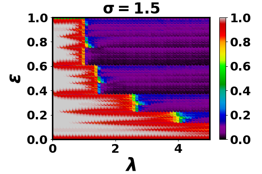
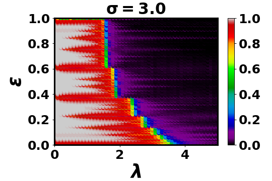
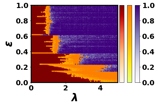
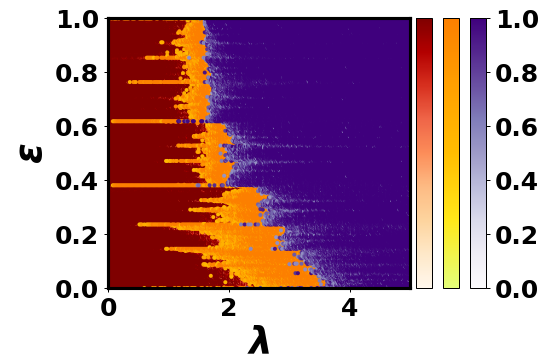
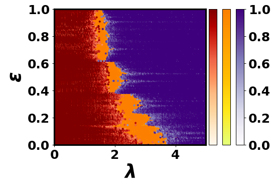
We begin our analysis by calculating the multifractal dimension as a function of disorder strength for all the single particle eigenstates of the LRH Hamiltonian for and as shown in Fig. 4(a)–4(c) respectively. In the case of , with an increase in disorder strength, the fraction of delocalized eigenstates decreases, and multifractal states are observed to appear in blocks, as shown in Fig. 4(a). Thus a delocalized-to-multifractal (DM) edge is observed in the eigenstate spectrum, which changes in a step-like fashion with increasing disorder strength . In the case of (see Fig. 4(b)) and (see Fig. 4(c)), we observe that the delocalized eigenstates are separated from the localized eigenstates, with a delocalized-to-localized (DL) edge which changes in a step-like fashion as the number of delocalized states decreases with increasing disorder strength . We also observe the presence of multifractal states in the vicinity of the DM / DL edges.
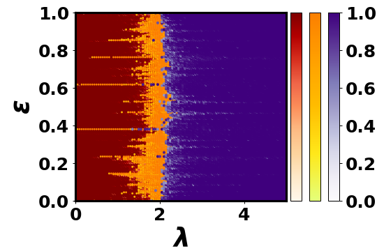
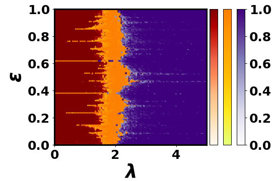
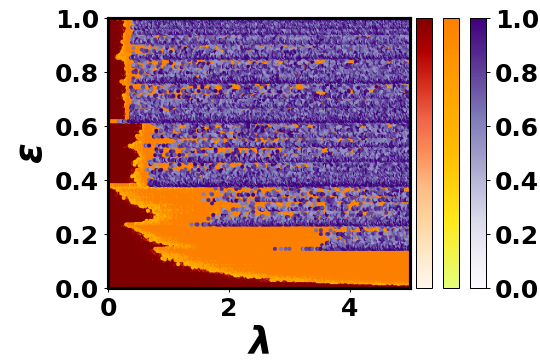
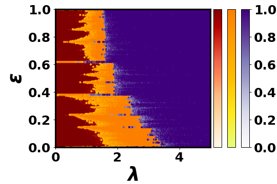
We next employ the multi-class classification algorithm for a single disorder realization and compare its performance with the multifractal analysis. First, the network (see Fig. 1) is trained using the eigenstates of the LRH model generated over multiple disorder realizations for various values of . We assign the class to the vectors in the training data set with the help of using Eq. 11. The phase diagram obtained as a function of disorder strength using the neural network for a single disorder realization is shown in Fig. 4(d)–4(f) corresponding to and respectively. The states are classified as delocalized, multifractal and localized with confidence and , respectively. In all figures, we have plotted the where the red, orange and purple colour codes are used to represent , , and respectively. Comparing Figs. 4(a)–4(c) with Figs. 4(d)–4(f), we observe that the shape and location of the transitions agree very well at all values of .
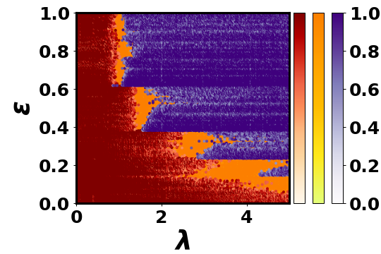
Next, we compare the neural network-based transition characterization when the same network (see Fig. 1) is trained using the eigenstates of the AAH model. Although the existence of a critical disorder strength at which all eigenstates are multifractal and separate the delocalized and localized eigenstates is well-known, we still assign the class to the vectors in the training data set with the help of using Eq. 11. Once the network is trained, we utilize it to obtain the phase diagrams of the LRH model as a function of disorder strength using the neural network for a single disorder realization as shown in Fig. 4(g)–4(i) corresponding to and respectively. While the network can precisely predict the location of the transitions/steps, the distinction between the delocalized and multifractal states is not very sharp. Nevertheless, we still observe the step-like features and the distinct phases.
We next compute the multifractal dimension as a function of disorder strength for all the single particle eigenstates of the AAH model (see Fig. 5(a)). All the eigenstates are delocalized for while all eigenstates are localized for . At , the eigenstates are multifractal [52, 51]. We obtain the phase diagram of the AAH model using the neural network trained on the eigenstates of the LRH model (see Fig. 5(b)) and the eigenstates of the AAH model (see Fig. 5(c)). The neural network can accurately predict the phase diagram using a single disorder realization in both cases. We also checked that a network trained with a higher-order fractal dimension like is also able to faithfully reproduce the phase diagram as shown in the Appendix.
(a)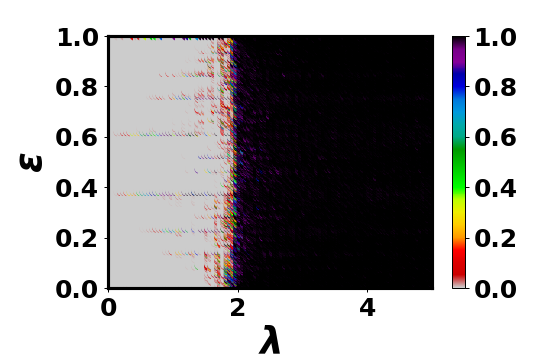 \stackunder(b)
(a)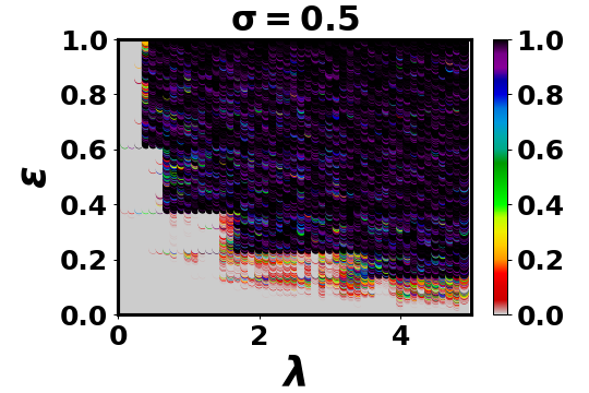 \stackunder(b)
 \stackunder(c)
IV.2 Binary classification
In this subsection, we discuss the results obtained with a binary classifier using the neural network shown in Fig. 3. The training data set consists of the probability densities (PDs) corresponding to the eigenstates of the two classes, i.e., delocalized () and localized (). Since we have a single neuron in the output layer, the output represents the probability of the state being localized, implying that is the probability of the state being delocalized. We may infer that intermediate values of indicate that the state exhibits multifractal nature.
The information about the transition from the delocalized to localized regimes is incorporated in the properties of the eigenstates. We feed the central eigenstate (corresponding to the energy of the spectrum) to the trained network to determine the transition point. In Fig. 6, we have plotted the classification prediction as a function of disorder strength . The transition point is revealed to be at as the network learns the difference between the localized and delocalized eigenstates. The transition point obtained agrees with the one shown using multifractal dimension in Fig. 5(a).
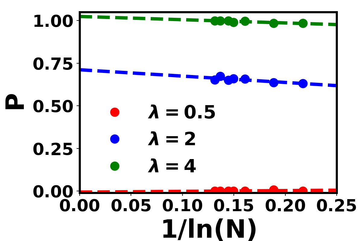
Next, we test this trained neural network, by inputting the probability densities drawn from all the eigenstates of the AAH model, as is varied across the transition. The neural network gives a single output , which signifies the confidence of the network to classify the state as localized, indicating that is the probability of classifying the state as delocalized. For a single disorder realization, the phase diagram obtained from the neural network shown in Fig. 7(a) is consistent with the one obtained using multifractal dimension as shown in Fig. 5(a). We also note that at the transition point where the multifractal states exist, the prediction lies roughly midway between and , consistent with theoretical results. In Fig. 7(b), we numerically study the system-size dependence [36] of the probability of the eigenstates being localized obtained using the binary classifier. While in the delocalized phase at , remains close to , at the multifractal point , it lies between and . In the localized phase with , approaches unity. This analysis is consistent with the ones obtained using conventional methods and can be utilized in classifying phases robustly against increasing system sizes.
Next, we implement the binary classification algorithm on the LRH model to investigate how well our neural network can identify a previously unknown phase. Since the network is trained exclusively on the delocalized and localized phases, it is unfamiliar with the multifractal regime. In Fig. 8(a)–8(c), we have plotted the phase diagram by feeding the eigenstates of a single disorder realization of the LRH model to the binary classifier corresponding to and respectively. We observe that our network can indicate the presence of a new phase (multifractal phase). In Fig. 8(a), for , while the network shows confusion in the multifractal phase, the step-like features that distinctly separate the delocalized states can still be observed. In Fig. 8(b)–(c), for and , we observe that the delocalized and localized states are classified and separated by step-like edges along which multifractal states are observed with . In other words, while the network identifies the delocalized and localized phases, in the case of the multifractal phase, it cannot clearly distinguish it from the localized phase. This inability of the network to produce results similar to multi-class classification is expected; as a matter of fact, the close connection between the phase diagram obtained by the binary classifer to the actual one is quite remarkable.
V Conclusion
In this work, we explore the ability of artificial neural networks to extract information about various phases from single-particle states. We build a multi-layer perceptron network and employ it to classify the delocalized, multifractal and localized phases of the quasiperiodic long-range Harper model. Our neural network produces phase diagrams that align with theoretical predictions after being trained using the data associated with the three phases. We establish that the machine successfully learns each phase’s property from the eigenstates. The machine has high confidence throughout all the phases, which is an indication of good feature extraction.
We also build a binary classifier with a single hidden layer having probability densities of the eigenstates of the AAH model as inputs to identify the delocalized and localized regimes. When we test this neural network with the AAH model, we find that the resulting phase diagram agrees very closely with the theoretically known phase diagram. Even though the network is not trained with multifractal states, the phase diagram obtained indicates the presence of multifractal states, in a manner very similar to the actual phase diagram. Subsequently, the network is applied to the LRH model for detecting an unlearned phase. The neural network shows confusion, whenever multifractal states are involved; however the phase diagram obtained is remarkably close to the actual one. In this work, we can obtain the phase diagrams with reasonable accuracy by feeding a single disorder realization to the trained neural network. Thus, the neural network method provides an alternative to the known conventional methods. Also, in recent times several works have explored the implementation of machine learning techniques in the context of many-body quantum systems [20, 23, 24, 25, 26, 17, 6]. A possible extension of our current work would be to identify and distinguish various phases in the many-body interacting system once the neural network learns the characteristics of the many-body wavefunctions in the different phases.
The phase classification problems in the literature have primarily focused on binary classification. In this context, investigating multiple phase transitions and training partially blind networks to recognize unknown phases remains unexplored. The value of this multi-neuron output strategy will be much more significant when dealing with novel phases for which acceptable order parameters are not known in advance.
Acknowledgements.
A.A. is grateful to the Council of Scientific and Industrial Research (CSIR), India, for her PhD fellowship. A.S. acknowledges financial support from SERB via the grant (File Number: CRG/2019/003447) and DST via the DST-INSPIRE Faculty Award [DST/INSPIRE/04/2014/002461]. All neural networks used in this work were implemented in Python using TENSORFLOW [70].Appendix A 3-D Anderson model
In this section, we employ the binary classifier to plot the phase diagram of the D Anderson model [32]. In particular, we train the neural network (shown in Fig. 3) by utilizing the eigenstate probabilities of the D AAH model (Eq. 2) with sites. Since the dimension of the neural network’s input layer is , we consider a cubic lattice with sites to obtain the network’s prediction. The Hamiltonian of the D Anderson model is:
| (12) |
where the on-site energies are drawn from a uniform random distribution and is the disorder parameter. Here, is set as unity.
(a)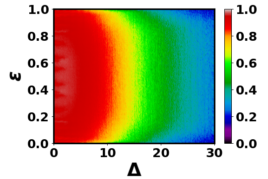 \stackunder(b)
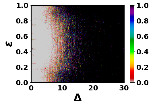
In Fig 9(a), we plot the phase diagram of the D Anderson model, with increasing strength of disorder and the color denoting the multifractal dimension . Above the critical disorder strength [71], all the eigenstates are exponentially localized with close to zero. At sub-critical disorder strengths, localized and extended states are observed, separated by some critical energy, dubbed the mobility edge [72]. We employ the binary classifier by training it on all the eigenstates of the AAH model at the disorder strengths (delocalized phase) and (localized). The resulting network is then used to predict the phase diagram of the Anderson model, as shown in Fig. 9(b). We observe that the network precisely identifies the delocalized eigenstates with , the mobility edges with , separating the delocalized and localized eigenstates as well as the critical disorder strength beyond which all the eigenstates are localized with close to unity. Thus, the network predicts the phase diagram of a system subjected to random disorder with reasonable accuracy despite the fact that it was trained on the eigenstates of a system with a quasiperiodic disorder and whose geometry is set in a different dimension.
(a)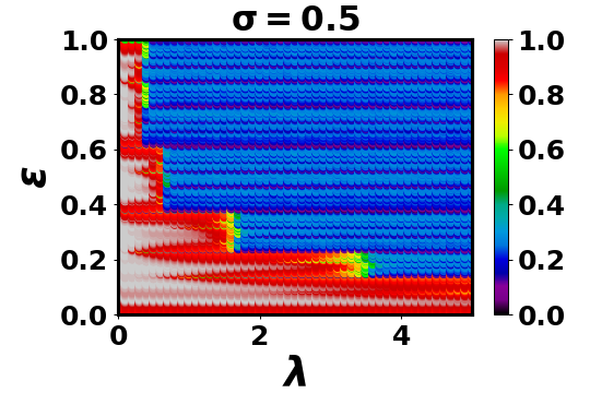 \stackunder(b)
(c)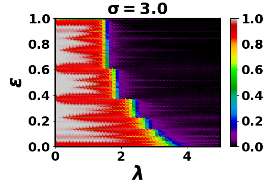 \stackunder(d)
(e)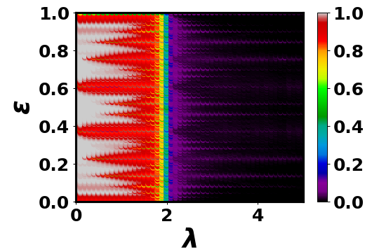 \stackunder(f)
Appendix B Higher order fractal dimension
In this section, we utilize higher-order fractal dimension (see Eq. 9) to label the eigenstates as delocalized, localized and multifractal in order to train the neural networks. For each eigenstate, the fractal dimension is calculated and labelled as follows:
| Localized, | ||||
| Multifractal, | ||||
| (13) |
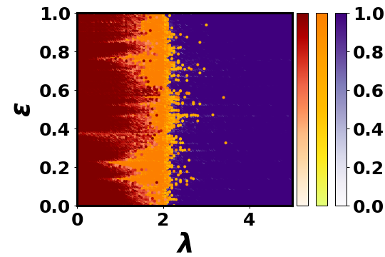
In Figs. 10(a) and 10(c) we have calculated as a function of disorder strength for all the single particle eigenstates for the long-range hopping parameter and . The corresponding phase diagrams plotted using the multi-class classification neural network trained using the eigenstates of the LRH model where the class is assigned using are shown in Figs. 10(b) and 10(d). We next compute the multifractal dimension as a function of disorder strength for all the single particle eigenstates of the AAH model (see Fig. 10(e)). The corresponding phase diagram obtained using the neural network trained on the eigenstates of the LRH model is shown in Fig. 10(f). We observe that even when the network is trained on the eigenstates labelled using higher moments, such as , it classifies the various phases with reasonable accuracy, as well as precisely predicts the location of the transitions/steps. This implies that any quantity which reflects the localization properties of the system can be used for labelling data in supervised machine learning.
References
- Jordan and Mitchell [2015] M. I. Jordan and T. M. Mitchell, Machine learning: Trends, perspectives, and prospects, Science 349, 255 (2015), https://www.science.org/doi/pdf/10.1126/science.aaa8415 .
- Carleo et al. [2019] G. Carleo, I. Cirac, K. Cranmer, L. Daudet, M. Schuld, N. Tishby, L. Vogt-Maranto, and L. Zdeborová, Machine learning and the physical sciences, Rev. Mod. Phys. 91, 045002 (2019).
- Ippoliti et al. [2017] M. Ippoliti, S. D. Geraedts, and R. N. Bhatt, Connection between fermi contours of zero-field electrons and composite fermions in two-dimensional systems, Phys. Rev. B 96, 045145 (2017).
- Ramprasad et al. [2017] R. Ramprasad, R. Batra, G. Pilania, A. Mannodi-Kanakkithodi, and C. Kim, Machine learning in materials informatics: recent applications and prospects - npj Computational Materials, https://www.nature.com/articles/s41524-017-0056-5 (2017).
- Ch’ng et al. [2017] K. Ch’ng, J. Carrasquilla, R. G. Melko, and E. Khatami, Machine learning phases of strongly correlated fermions, Phys. Rev. X 7, 031038 (2017).
- Schindler et al. [2017] F. Schindler, N. Regnault, and T. Neupert, Probing many-body localization with neural networks, Phys. Rev. B 95, 245134 (2017).
- Wetzel and Scherzer [2017] S. J. Wetzel and M. Scherzer, Machine learning of explicit order parameters: From the ising model to su(2) lattice gauge theory, Phys. Rev. B 96, 184410 (2017).
- Wetzel [2017] S. J. Wetzel, Unsupervised learning of phase transitions: From principal component analysis to variational autoencoders, Phys. Rev. E 96, 022140 (2017).
- Wang [2016] L. Wang, Discovering phase transitions with unsupervised learning, Phys. Rev. B 94, 195105 (2016).
- Liu and van Nieuwenburg [2018] Y.-H. Liu and E. P. L. van Nieuwenburg, Discriminative cooperative networks for detecting phase transitions, Phys. Rev. Lett. 120, 176401 (2018).
- Broecker et al. [2017a] P. Broecker, F. F. Assaad, and S. Trebst, Quantum phase recognition via unsupervised machine learning (2017a).
- Hu et al. [2017] W. Hu, R. R. P. Singh, and R. T. Scalettar, Discovering phases, phase transitions, and crossovers through unsupervised machine learning: A critical examination, Phys. Rev. E 95, 062122 (2017).
- Cadez et al. [2023] T. Cadez, B. Dietz, D. Rosa, A. Andreanov, K. Slevin, and T. Ohtsuki, Machine learning wave functions to identify fractal phases (2023), arXiv:2306.01402 [cond-mat.dis-nn] .
- Liu et al. [2017] J. Liu, Y. Qi, Z. Y. Meng, and L. Fu, Self-learning monte carlo method, Phys. Rev. B 95, 041101 (2017).
- Huang and Wang [2017] L. Huang and L. Wang, Accelerated monte carlo simulations with restricted boltzmann machines, Phys. Rev. B 95, 035105 (2017).
- Wang [2017] L. Wang, Exploring cluster monte carlo updates with boltzmann machines, Phys. Rev. E 96, 051301 (2017).
- Carleo and Troyer [2017a] G. Carleo and M. Troyer, Solving the quantum many-body problem with artificial neural networks, Science 355, 602 (2017a), https://www.science.org/doi/pdf/10.1126/science.aag2302 .
- Glasser et al. [2018] I. Glasser, N. Pancotti, M. August, I. D. Rodriguez, and J. I. Cirac, Neural-network quantum states, string-bond states, and chiral topological states, Phys. Rev. X 8, 011006 (2018).
- Lu et al. [2019] S. Lu, X. Gao, and L.-M. Duan, Efficient representation of topologically ordered states with restricted boltzmann machines, Phys. Rev. B 99, 155136 (2019).
- Carleo et al. [2018] G. Carleo, Y. Nomura, and M. Imada, Constructing exact representations of quantum many-body systems with deep neural networks, Nature Communications 9 (2018).
- Torlai et al. [2018] G. Torlai, G. Mazzola, J. Carrasquilla, M. Troyer, R. Melko, and G. Carleo, Neural-network quantum state tomography, Nature Physics 14, 447 (2018).
- Cai and Liu [2018] Z. Cai and J. Liu, Approximating quantum many-body wave functions using artificial neural networks, Physical Review B 97 (2018).
- Gardas et al. [2018] B. Gardas, M. M. Rams, and J. Dziarmaga, Quantum neural networks to simulate many-body quantum systems, Physical Review B 98 (2018).
- Carrasquilla and Torlai [2021] J. Carrasquilla and G. Torlai, How To Use Neural Networks To Investigate Quantum Many-Body Physics, PRX Quantum 2 (2021).
- Schmitt and Heyl [2020] M. Schmitt and M. Heyl, Quantum Many-Body Dynamics in Two Dimensions with Artificial Neural Networks, Physical Review Letters 125 (2020).
- Carleo and Troyer [2017b] G. Carleo and M. Troyer, Solving the quantum many-body problem with artificial neural networks, Science 355, 602 (2017b).
- [27] P. Cunningham, M. Cord, and S. J. Delany, Supervised Learning, https://link.springer.com/chapter/10.1007/978-3-540-75171-7_2.
- Broecker et al. [2017b] P. Broecker, J. Carrasquilla, R. G. Melko, and S. Trebst, Machine learning quantum phases of matter beyond the fermion sign problem, Scientific Reports 7, 8823 (2017b).
- Zhang and Kim [2017] Y. Zhang and E.-A. Kim, Quantum loop topography for machine learning, Phys. Rev. Lett. 118, 216401 (2017).
- Ohtsuki and Ohtsuki [2016] T. Ohtsuki and T. Ohtsuki, Deep learning the quantum phase transitions in random two-dimensional electron systems, Journal of the Physical Society of Japan 85, 123706 (2016), https://doi.org/10.7566/JPSJ.85.123706 .
- Zhang et al. [2018] P. Zhang, H. Shen, and H. Zhai, Machine learning topological invariants with neural networks, Phys. Rev. Lett. 120, 066401 (2018).
- Anderson [1958] P. W. Anderson, Absence of diffusion in certain random lattices, Phys. Rev. 109, 1492 (1958).
- Goldman and Kelton [1993] A. I. Goldman and R. F. Kelton, Quasicrystals and crystalline approximants, Rev. Mod. Phys. 65, 213 (1993).
- Kohmoto et al. [1987] M. Kohmoto, B. Sutherland, and C. Tang, Critical wave functions and a cantor-set spectrum of a one-dimensional quasicrystal model, Phys. Rev. B 35, 1020 (1987).
- Ahmed et al. [2021] A. Ahmed, N. Roy, and A. Sharma, Dynamics of spectral correlations in the entanglement hamiltonian of the aubry-andré-harper model, Phys. Rev. B 104, 155137 (2021).
- Ahmed et al. [2022] A. Ahmed, A. Ramachandran, I. M. Khaymovich, and A. Sharma, Flat band based multifractality in the all-band-flat diamond chain, Phys. Rev. B 106, 205119 (2022).
- Ahmed et al. [2023] A. Ahmed, N. Roy, and A. Sharma, Interplay of many-body interactions and quasiperiodic disorder in the all-band-flat diamond chain (2023), arXiv:2303.17633 [cond-mat.dis-nn] .
- Aubry and André [1980] S. Aubry and G. André, Analyticity breaking and Anderson localization in incommensurate lattices, Ann. Israel Phys. Soc. 3, 18 (1980).
- Harper [1955] P. G. Harper, Single band motion of conduction electrons in a uniform magnetic field, Proceedings of the Physical Society. Section A 68, 874 (1955).
- Lima et al. [2004] R. P. A. Lima, H. R. da Cruz, J. C. Cressoni, and M. L. Lyra, Finite-size scaling of power-law bond-disordered anderson models, Phys. Rev. B 69, 165117 (2004).
- Mirlin et al. [1996] A. D. Mirlin, Y. V. Fyodorov, F.-M. Dittes, J. Quezada, and T. H. Seligman, Transition from localized to extended eigenstates in the ensemble of power-law random banded matrices, Phys. Rev. E 54, 3221 (1996).
- Deng et al. [2018] X. Deng, V. E. Kravtsov, G. V. Shlyapnikov, and L. Santos, Duality in power-law localization in disordered one-dimensional systems, Phys. Rev. Lett. 120, 110602 (2018).
- Deng et al. [2019] X. Deng, S. Ray, S. Sinha, G. V. Shlyapnikov, and L. Santos, One-dimensional quasicrystals with power-law hopping, Phys. Rev. Lett. 123, 025301 (2019).
- Gopalakrishnan [2017] S. Gopalakrishnan, Self-dual quasiperiodic systems with power-law hopping, Phys. Rev. B 96, 054202 (2017).
- Roy and Sharma [2021] N. Roy and A. Sharma, Fraction of delocalized eigenstates in the long-range aubry-andré-harper model, Phys. Rev. B 103, 075124 (2021).
- JANSSEN [1994] M. JANSSEN, Multifractal ANALYSIS OF BROADLY-DISTRIBUTED OBSERVABLES AT CRITICALITY, International Journal of Modern Physics B 08, 943 (1994).
- Schreiber and Grussbach [1991] M. Schreiber and H. Grussbach, Multifractal wave functions at the Anderson transition, Physical Review Letters 67, 607 (1991).
- Brezini [1985] A. Brezini, Localization in one-dimensional random potential, in Volume 128, Number 1 March 1 (De Gruyter, Berlin, Boston, 1985) pp. 439–444.
- Beeby and Mott [1964] J. L. Beeby and N. F. Mott, The electronic structure of disordered system, Proceedings of the Royal Society of London. Series A. Mathematical and Physical Sciences 279, 82 (1964).
- Bohigas et al. [1984] O. Bohigas, M. J. Giannoni, and C. Schmit, Characterization of chaotic quantum spectra and universality of level fluctuation laws, Phys. Rev. Lett. 52, 1 (1984).
- Modugno [2009] M. Modugno, Exponential localization in one-dimensional quasi-periodic optical lattices, New Journal of Physics 11, 033023 (2009).
- Evers and Mirlin [2008] F. Evers and A. D. Mirlin, Anderson transitions, Rev. Mod. Phys. 80, 1355 (2008).
- Thouless [1983] D. J. Thouless, Bandwidths for a quasiperiodic tight-binding model, Phys. Rev. B 28, 4272 (1983).
- McCulloch and Pitts [1943] W. S. McCulloch and W. Pitts, A logical calculus of the ideas immanent in nervous activity, The bulletin of mathematical biophysics 5 (1943).
- Rosenblatt [1958] F. Rosenblatt, The perceptron: A probabilistic model for information storage and organization in the brain, Psychological Review 65, 386–408 (1958).
- Bishop [2006] C. M. Bishop, Pattern Recognition and Machine Learning (2006).
- Dubey et al. [2021] S. R. Dubey, S. K. Singh, and B. B. Chaudhuri, Activation functions in deep learning: A comprehensive survey and benchmark (2021).
- Goodfellow et al. [2016a] I. J. Goodfellow, Y. Bengio, and A. Courville, Deep Learning (MIT Press, Cambridge, MA, USA, 2016) http://www.deeplearningbook.org.
- Srivastava et al. [2014] N. Srivastava, G. Hinton, A. Krizhevsky, I. Sutskever, and R. Salakhutdinov, Dropout: A simple way to prevent neural networks from overfitting, Journal of Machine Learning Research 15, 1929 (2014).
- Fukushima [1975] K. Fukushima, Cognitron: A self-organizing multilayered neural network - Biological Cybernetics, https://link.springer.com/article/10.1007/BF00342633 (1975).
- Feng and Lu [2019] J. Feng and S. Lu, Performance Analysis of Various Activation Functions in Artificial Neural Networks, Journal of Physics: Conference Series 1237, 022030 (2019).
- Agarap [2019] A. F. Agarap, Deep learning using rectified linear units (relu) (2019), arXiv:1803.08375 [cs.NE] .
- Goodfellow et al. [2016b] I. Goodfellow, Y. Bengio, and A. Courville, Deep Learning (MIT Press, 2016) http://www.deeplearningbook.org.
- Rumelhart et al. [1986] D. E. Rumelhart, G. E. Hinton, and R. J. Williams, Learning representations by back-propagating errors, Nature 323, 533 (1986).
- Kingma and Ba [2014] D. P. Kingma and J. Ba, Adam: A method for stochastic optimization (2014).
- Song et al. [2016] Y. Song, A. G. Schwing, R. S. Zemel, and R. Urtasun, Training deep neural networks via direct loss minimization (2016), arXiv:1511.06411 [cs.LG] .
- Lindinger et al. [2019] J. Lindinger, A. Buchleitner, and A. Rodríguez, Many-body multifractality throughout bosonic superfluid and Mott insulator phases, Phys. Rev. Lett. 122, 106603 (2019).
- Macé et al. [2019] N. Macé, F. Alet, and N. Laflorencie, Multifractal scalings across the many-body localization transition, Phys. Rev. Lett. 123, 180601 (2019).
- Wang et al. [2016] Y. Wang, Y. Wang, and S. Chen, Spectral statistics, finite-size scaling and multifractal analysis of quasiperiodic chain with p-wave pairing, The European Physical Journal B 89, 254 (2016).
- Abadi et al. [2015] M. Abadi, A. Agarwal, P. Barham, E. Brevdo, Z. Chen, C. Citro, G. Corrado, A. Davis, J. Dean, M. Devin, S. Ghemawat, I. Goodfellow, A. Harp, G. Irving, M. Isard, Y. Jia, R. Jozefowicz, L. Kaiser, M. Kudlur, J. Levenberg, D. Mané, R. Monga, S. Moore, D. Murray, C. Olah, M. Schuster, J. Shlens, B. Steiner, I. Sutskever, K. Talwar, P. Tucker, V. Vanhoucke, V. Vasudevan, F. Viégas, O. Vinyals, P. Warden, M. Wattenberg, M. Wicke, Y. Yu, and X. Zheng, Tensorflow: Large-scale machine learning on heterogeneous distributed systems (2015).
- Mott [1968] N. Mott, Conduction in glasses containing transition metal ions, Journal of Non-Crystalline Solids 1, 1 (1968).
- [72] Anderson Localization and Its Ramifications, https://link.springer.com/book/10.1007/b13139.