MINN: Learning the dynamics of differential-algebraic equations and application to battery modeling

Abstract

The concept of integrating physics-based and data-driven approaches has become popular for modeling sustainable energy systems. However, the existing literature mainly focuses on the data-driven surrogates generated to replace physics-based models. These models often trade accuracy for speed but lack the generalisability, adaptability, and interpretability inherent in physics-based models, which are often indispensable in the modeling of real-world dynamic systems for optimization and control purposes. In this work, we propose a novel architecture for generating model-integrated neural networks (MINN) to allow integration on the level of learning physics-based dynamics of the system. The obtained hybrid model solves an unsettled research problem in control-oriented modeling, i.e., how to obtain an optimally simplified model that is physically insightful, numerically accurate, and computationally tractable simultaneously. We apply the proposed neural network architecture to model the electrochemical dynamics of lithium-ion batteries and show that MINN is extremely data-efficient to train while being sufficiently generalizable to previously unseen input data, owing to its underlying physical invariants. The MINN battery model has an accuracy comparable to the first principle-based model in predicting both the system outputs and any locally distributed electrochemical behaviors but achieves two orders of magnitude reduction in the solution time.

1 Introduction

Rapid advances in electromobility have positioned battery as a key player in the transition towards a more sustainable future, with its impact on carbon neutrality continuing to gain momentum. While most battery research has been mainly focused on searching for novel materials [1, 2], the established battery chain and its circular economy have been dominated by lithium-ion batteries (LIBs) foreseen to prevail due to their proven long-term stability, cost-effective production and recycling. Consequently, the pressure of electromobility has been put on the optimization of LIBs in the foreseeable future, from cell-level chemistry, structure, and manufacturing process to system-level solutions for improved safety, reliability, performance, and lifetime. One key limiting factor in unleashing the full potential of LIBs for electromobility is the current battery management systems (BMS), which limit the usage by putting more or less fixed constraints on battery cell external measurements. The next-generation BMS should enable accurate monitoring and optimal control of dynamical local behaviors distributed inside each cell for real-time optimized utilization of the battery systems.

A battery is a compact, multiphysics system with multiple state variables, domains, material phases and physical parameters over disparate time- and length scales. The current strategies for probing battery internal states involve battery modeling based on equivalent circuits, which at their best, are able to mimic the battery electric behaviors under specific conditions [3]. More sophisticated electrochemical models for locally distributed internal states, proven accurate in various usage conditions, are practically prohibitive to implement in BMS. Although the electrochemical models have been driving a wealth of LIB research in system identification [4, 5], state estimation [6, 7], fault and aging predictions [8, 9], and optimal control [10, 11], their typical end-user applications, such as smartphones and laptop computers, still require considerable computational power due to the highly nonlinear and stiff partial differential-algebraic equations (PDAEs), let alone the upscaling to pack-level and vehicle fleet-level battery applications. Despite numerous offline implementations employing state-of-the-art numerical techniques [12, 13, 14, 15, 16], it is still infeasible to consider advanced electrochemical models for on-board battery management with current hardware.

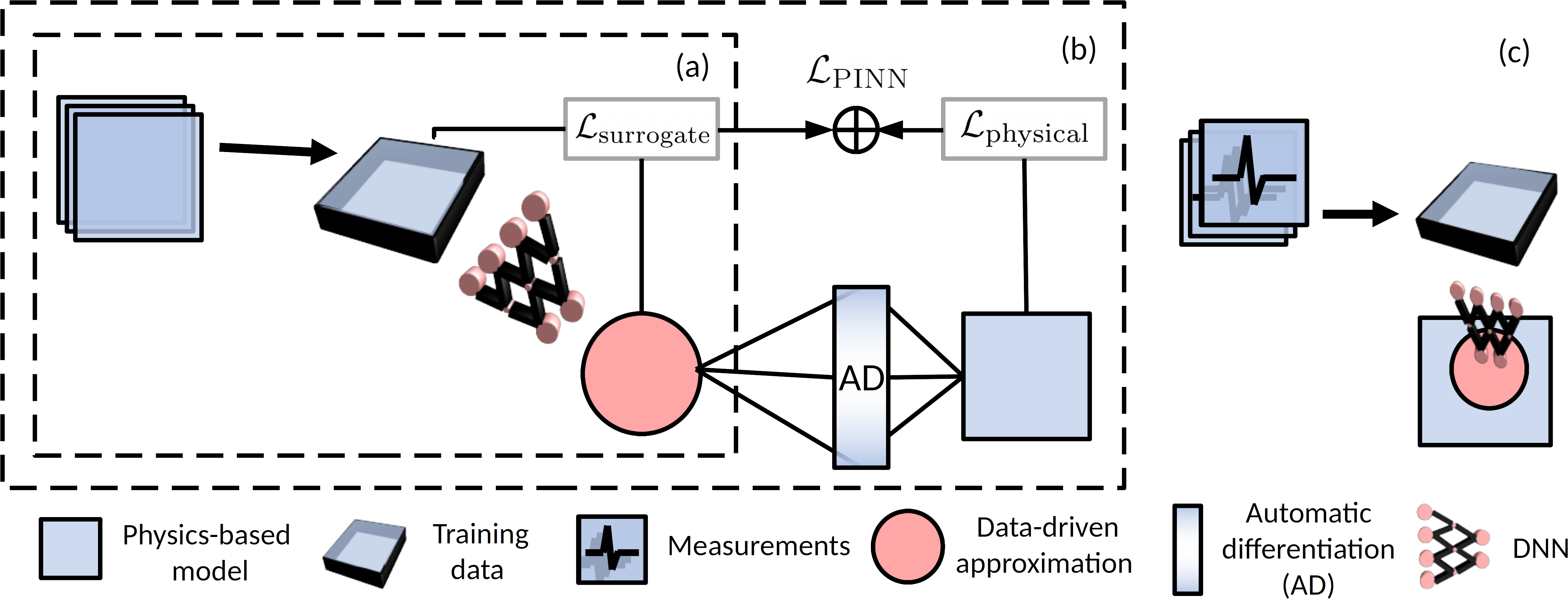
Figure 1: Existing physics-based integration strategies for the blending of neural networks and physics-based models in order to retain their individual merits. (a) A data-driven surrogate model using supervised learning requires relevant and representative training data generated by snapshots of the physics-based model solutions. (b) A surrogate model regularised physical constraints within the PINN framework, of which the PINN loss, $\mathcal{L}_{\text{PINN}}$, is composed of the loss due to model-data inconsistency, $\mathcal{L}_{\text{surrogate}}$, and the loss owing to physical constraints, $\mathcal{L}_{\text{physical}}$. (c) The PINN workflow for inverse problems used to identify physical parameters as part of parametric PDEs [17].

The fundamental challenges in solving PDAEs for control-oriented applications have been commonly addressed by reduced-order modeling. These reduced-order models (ROMs) attempt to lower the computational complexity by either exploring the mathematical structure of the governing equations or simplifying the physics of the original model. For example, the single particle model [18] features cell-interior variables derived from volume-averaged active materials and uniform molar flux, which result in systems of partial differential equations (PDEs). Other ROMs, such as the physics-based equivalent circuit model [19, 20], also result in a simplified system with fewer assumptions. On a high level, these model reduction strategies can be seen as an attempt to replace the original PDAE formulation with a simplified system, resulting in less computational complexity and fewer parameters but compromising accuracy under performance-limiting conditions.

The PDAE models, with their minimal assumptions and greater flexibility, offer a distinct advantage over other battery models by providing higher accuracy under a broader range of usage conditions. This makes them an ideal choice for all-purpose and comprehensive battery modeling. In practice, however, they are computationally too demanding for control-oriented applications, which hinders their adoption in BMS. Therefore, large efforts have been made to accelerate the solution process. Data-driven approaches have emerged as powerful tools to circumvent the stiffness issues associated with the first-principle electrochemical models by identifying high-dimensional patterns in battery data. For example, the cycle life of batteries can be accurately predicted using machine learning methods given enough relevant data [21, 22, 23] and fast estimations of the terminal voltage and state of charge (SOC) can be achieved by using recurrent neural networks (RNN) [24]. Nevertheless, training a purely data-driven model to predict the undetectable states of battery cells, such as the electrolyte concentration, local temperature and lithium plating potential, is obscured under such approaches due to the lack of measurements. However, these internal states are highly important for battery safety, health and optimal control purposes. Without tracking those, lithium dendrites may ultimately cause internal short-circuits to grow rapidly under conditions of electrolyte depletion [25], high temperature gradient [26] and negative plating potential [27]. Therefore, it is essential to include a set of the internal states in a battery model instead of the unphysical hidden states considered in an RNN-based battery model. As illustrated in Fig. 1(a), this class of models relies on generic neural networks that are agnostic to the underlying dynamics of the battery. In the presence of many trainable parameters in these neural network models, large and representable datasets are necessary for training to minimize out-of-sample errors, and those are, in turn, generated by physics-based models.

Physics-constrained learning offers a potential third way to blend neural networks with physics-based models. For example, physics-informed neural networks (PINNs) have successfully approximated the solutions to PDEs by adding physical constraints into the loss function [28]. As shown in Fig. 1(b), the PINN framework, enabled by automatic differentiation (AD), computes the residual of the PDE system in an unsupervised manner, leading to a loss term due to physical constraints, $\mathcal{L}_{\text{physical}}$, added to the supervised loss, $\mathcal{L}_{\text{surrogate}}$. For a small experimental dataset, the PINN framework allows for the approximation of intrinsic model parameters, which is illustrated in Fig. 1(c). This has been demonstrated to be effective even for stiff systems [29], and a suite of software tools targeting the automation of PINNs has made it accessible to different physical systems that can be formulated as an initial value problem [30, 31, 32]. However, the training of PINN can be costly due to the large degrees of freedom in approximating the spatiotemporal solution trajectory. It also has poor applicability to battery systems because of the time-varying inputs (e.g., applied current, voltage or temperature for battery systems), which alter the system dynamics in real time. Therefore, approximating the battery behaviors for an unpredictable battery cycle using PINN is impracticable.

To bridge the research gap, this work proposes a model-integrated deep learning framework, termed model-integrated neural networks (MINN), designed to leverage the approximation power of neural networks, and the physical insight and numerical machinery, from those of a physics-based model. MINN is shown to be extremely data-efficient to train and can extrapolate beyond the operating conditions considered in the training data. Furthermore, it retains the physical significance of hidden states and model parameters that can be used directly for system identification, model adaptation, state estimation, and model-based control of LIB. The generality of the proposed framework allows for the easy adoption of other dynamic systems.

2 Model-Integrated Neural Networks

The paradigm of integrating prior knowledge into a black box was introduced by the PINN framework and has two integration schemes, as depicted in Fig. 1(b) and 1(c). The possible failure modes of PINN and the inefficiency of training for long-time horizons have suggested sequence-to-sequence learning as opposed to learning the entire space-time solution [33]. Most importantly, the sequence-to-sequence learning approach has to allow for the incorporation of control inputs which overcomes the shortcomings of PINN when applied to the management and control of dynamical systems. Based on this idea, MINN is designed to integrate the physics-based equations into a neural network architecture directly, as shown in Fig. 2. The physics-based equations encode and capture the underlying physical invariants and domain-specific knowledge.

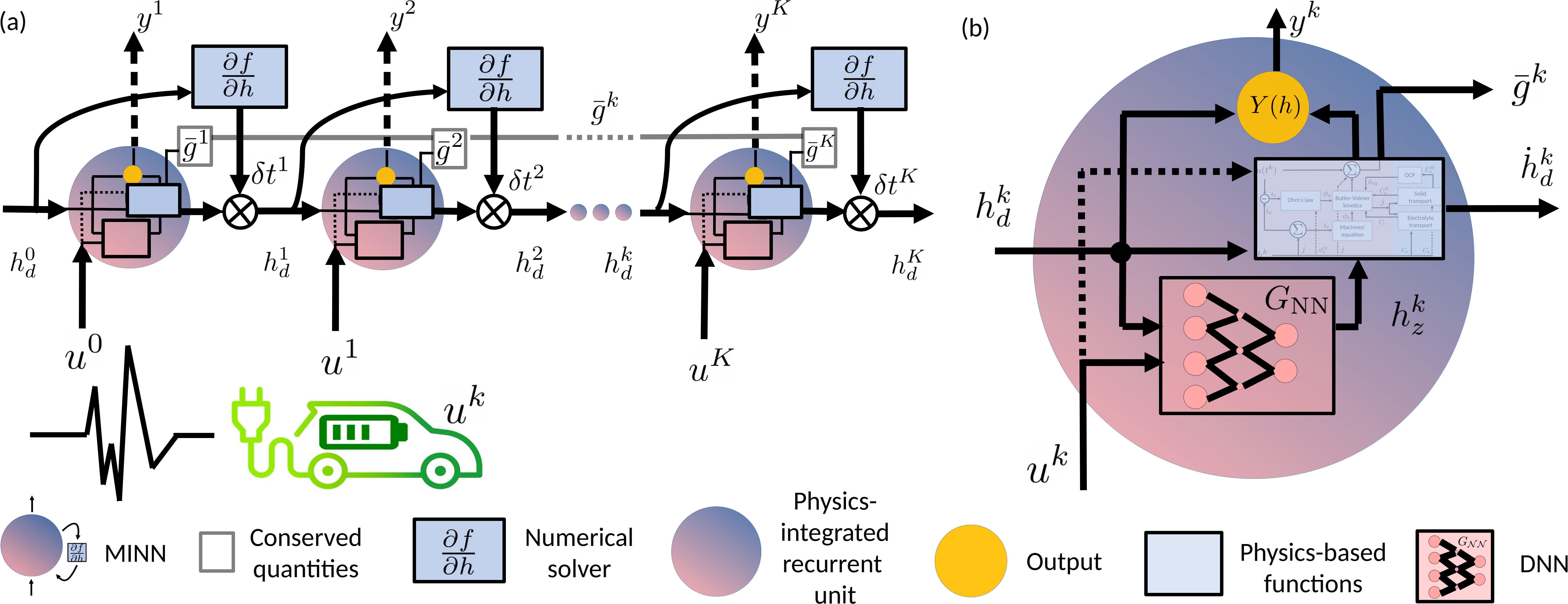
Figure 2: The proposed MINN architecture for dynamic systems. (a) An iterative update of the hidden states $h^{k}_{d}$, output $y^{k}$ and conserved quantities $\bar{g}^{k}$, is controlled by input $u(t^{k})$ at time $t^{k}$ through physics-based hidden units. The time stepping $\delta t^{k}$ is adaptive to the dynamics thanks to a skipping mechanism via the numerical solver. (b) The design of a physics-based hidden unit contains physics-based equations, a deep learning-enabled function $G_{\text{NN}}$ and an output function $Y$.

General multi-timescale dynamic systems can be formulated as coupled differential-algebraic equations (DAEs), resulting from the spatial discretization of the original PDAEs:

$$\dot{h}_{d}(t) =f\Big{(}t,h_{d},h_{z},u\Big{)},$$ (1)

$$y(t) =Y\Big{(}t,h_{d},h_{z},u\Big{)},$$ (2)

$$0 =g\Big{(}t,h_{d},h_{z},u\Big{)}.$$ (3)

The above DAE system features differential states $h_{d}$, algebraic variables $h_{z}$, and a time-varying control input $u$. $y$ is the output of interest, and $Y$ is the function to compute the output from the states and the input. The origin of the algebraic equation (3) is threefold, i.e., they can stem from the boundary conditions, the singular perturbation of the original PDAEs, or conservation laws naturally arising from the physical problem. In some special cases, explicit solutions for Eqn. (3) exist for $h_{z}$, which makes it replaceable by a function $G(t,h_{d},\,u)$ in Eqns. (1)- (2). However, in most cases, $h_{z}$ does not have a fixed-form solution in terms of $h_{d}$ and $u$. In such cases, more computationally involved DAE solvers must be used.

Due to the high computational cost of solving DAE systems, the solution process, or the model itself, must be simplified. If the end result of training PINNs is a fast solution and of numerical methods, a slow, coarse-grained solution, training MINN generates a simplified dynamic model, as shown in the schematics of MINN Fig. 2(a). To this end, we parameterize within the hidden unit an explicit function $G_{\text{NN}}$ for the algebraic variables in terms of the differential states $h_{d}$, the control input $u$, and neural network parameters $\theta$. For sequence-to-sequence learning, the MINN hidden states at time step $k+1$ can be updated by

$$h_{d}^{k+1} =f\,(t^{k},h_{d}^{k},h_{z}^{*,k},u^{k})\cdot\delta t^{k+1},$$ (4)

$$h_{z}^{*,k} =G_{\text{NN}}\,(t^{k},h_{d}^{k},\,u^{k};\theta),$$ (5)

where Eqn. (4), is the discretized form of the continuous-time dynamics (1) and the algebraic variables $h_{z}^{*}$ in Eqn. (5) are approximations to the roots of Eqn. (3). The function $G_{\text{NN}}$ offers a shortcut to solving the implicit algebraic equations of the DAE system. Furthermore, the time step $\delta t$ is adaptively adjusted by the ODE solver. The system output $y$ and the conserved quantities of the battery system $\bar{g}$ are computed by

$$y^{k} =Y(t^{k},h_{d}^{k},h_{z}^{*,k},u^{k}),$$ (6)

$$\bar{g}^{k} =g(t^{k},h_{d}^{k},h_{z}^{*,k},u^{k}),$$ (7)

where $\bar{g}$ is an approximation of $g$, computed at each time step. $\bar{g}$ does not strictly vanish due to the approximation error, determined by trainable parameters $\theta$. In addition, the proposed MINN framework integrates the differential equations of the PDAE system into the network architecture through the physics-based hidden recurrent units, as shown in Fig. 2(b).

The search for an optimally simplified model (4)-(6) is cast as the following nonlinear optimization problem

$$\text{arg }\min\limits_{\theta}\>\mathcal{L}_{\text{MINN}}\,(\theta\,;\,\lambda)=\mathcal{L}_{y}(\theta)+\lambda\mathcal{L}_{g}(\theta),$$ (8)

in which the physics-based hidden units are used to formulate a physics-constrained loss function with $\mathcal{L}_{y}$ and $\mathcal{L}_{g}$ given by

$$\mathcal{L}_{y}(\theta)=\sum_{k=0}^{K}\Bigg{(}Y\Big{(}t^{k},h_{d}^{k},h_{z}^{*,k},u^{k}\Big{)}-\hat{y}^{k}\Bigg{)}^{2}\,\delta t^{k},$$ (9)

$$\mathcal{L}_{g}(\theta)=\sum_{k=0}^{K}\,\Bigg{|}\,g\,\Big{(}t^{k},h_{d}^{k},\,G_{\text{NN}}(t^{k},h_{d}^{k},\,u^{k}),\,u^{k}\Big{)}\Bigg{|}\,\,\delta t^{k},$$ (10)

where $\hat{y}^{k}$ are measurements and $K$ is the number of samples in the time time-series. In the training of MINN, we seek parameters $\theta$ by solving for $h_{d}$ for a given profile $u^{k}$. The loss function comprises a term $\mathcal{L}_{g}$ to quantify physical inconsistency, which due to conservation laws, is a function of the algebraic variables, plus a loss associated with the (measurable) output of the dynamic system. During training, the parameterized loss function $\mathcal{L}_{\text{MINN}}\,(\theta)$ is minimized via a gradient-based optimizer, and the Lagrange multiplier $\lambda$ is updated iteratively by the steepest ascent. Once the MINN model is obtained, an array of ODE solvers can be readily employed to reproduce the system’s state dynamics controlled by an arbitrary profile $u^{k}$.

The overarching architecture of MINN is a blend of the recurrent neural network (RNN) and the residual neural network (ResNet). The MINN is physically informed of the dynamics of the hidden states $h$ by adding skip (residual) connections and input that model the dynamic system controlled by $u^{k}$. The skipping mechanism is controlled by an ODE solver, i.e., the time stepping $\delta t$ is determined by the Jacobian $\tfrac{\partial f}{\partial h}$. This allows established numerical solvers to be integrated into not only the model evaluation but also for efficient training via backpropagation through the ODE solver. At the same time, it facilitates the optimization to adaptively focus on steeper regions of the trajectory. Physically, the input $u^{k}$ and the hidden states $h_{d}^{k}$ at time step $k$ are fed into the hidden unit, resulting in the approximation of the (algebraic) hidden variables $h_{z}^{k}$ as well as the time derivative $\dot{h}_{d}^{k}$ computed by a deep neural network (DNN) and physics-based functions respectively. This allows an explicit and direct integration of the physics-based governing equations and the physically meaningful states into the MINN architecture. This is similar to a continuous-depth model [34] but interleaved with model-integrated recurrent units with control input, providing it with physical interpretations and extrapolating abilities. The recurrent units continuously transform the hidden states in a sequence-to-sequence manner and output a time series of the conserved quantities, $\bar{g}^{k}$.

3 Application to battery modeling

As motivated before, lithium-ion batteries represent a prevalent technology in electromobility and sustainable energy storage that are important forces in the fight against climate change. In this respect, BMS plays a crucial role in battery safety, reliability, sustainability, and dynamic performance. The central thesis for enabling advanced BMS is to develop a battery model that simultaneously preserves physical insights, accuracy and computational efficiency. To this end, the proposed MINN architecture is applied to the modeling of lithium-ion batteries, where each hidden state of the MINN is assigned to an electrochemical state of the first principle battery model. Depending on the application, the control $u$ can be the current $I$ for a battery system. The output may include the terminal voltage, SOC and lithium plating potential if a reference electrode is used. The training data generation for MINN involves only the output that can be measured using, e.g., a three-electrode cell setup. Here, instead of learning blindly from the training data as illustrated by the hybrid approach shown in Fig. 1(c), we integrate prior knowledge, i.e., the equations from the PDAE system into the neural network architecture. Fig. 3 shows the realization of the physics-based equations in the hidden unit of MINN, for which the circuitry is based on Newman’s P2D model.

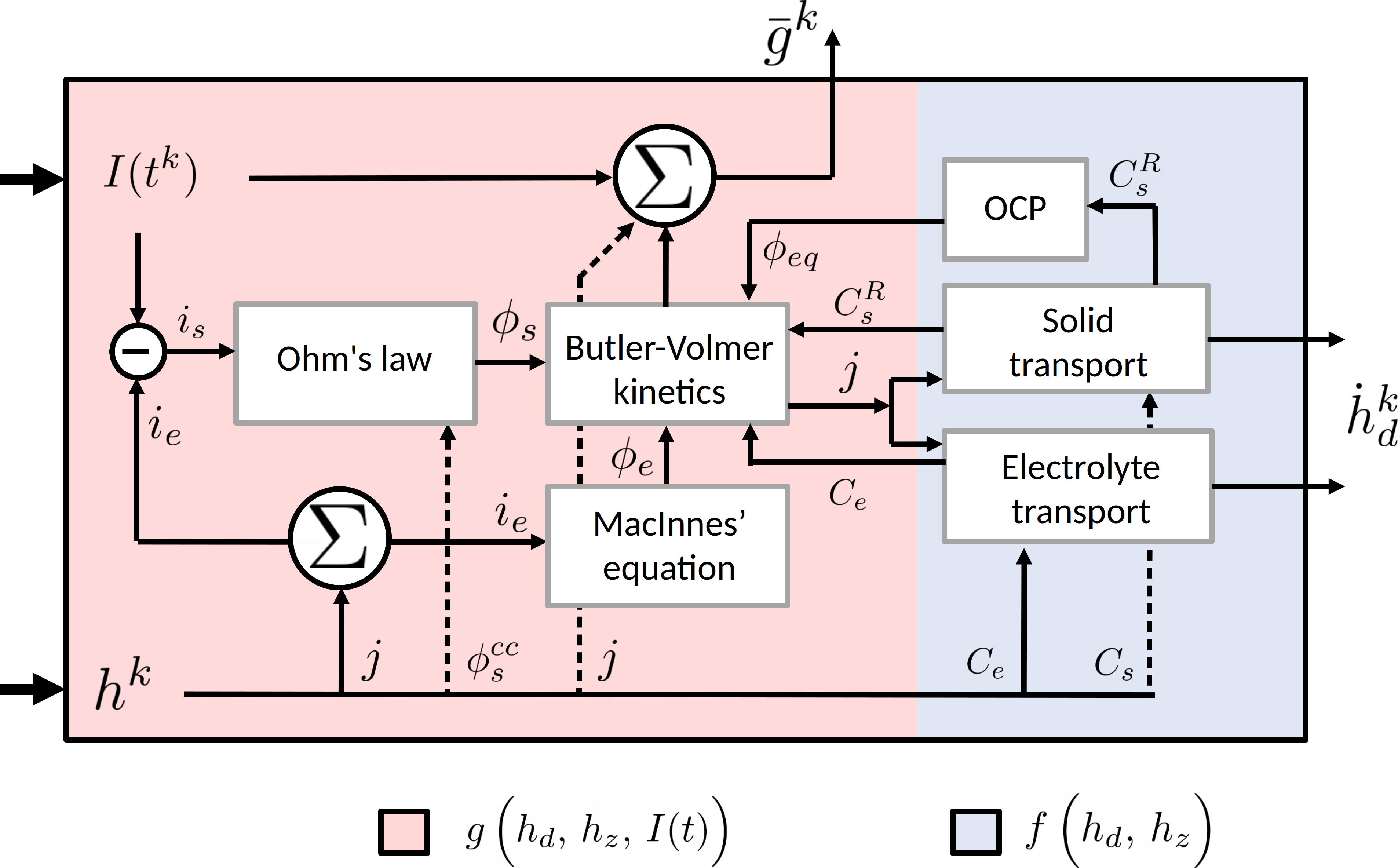
Figure 3: For battery modeling, the realization of the physics-based equations in the recurrent unit is marked by the blue rectangular in Fig. 2(b), which takes into account the domain knowledge of the physical system. It has the applied current $I$, differential states $h_{d}=[C_{s},\,C_{e}]^{T}$ and algebraic variables $h_{z}=j$ as inputs. The $g$-component evaluates the conservation laws at each time step $k$, while the $f$-component evaluates the time derivative of the differential states $\dot{h}_{d}$. The two components in the circuitry feature P2D equations, e.g., the open circuit potential (OCP) is a fitted function that takes in the solid concentration at the active material surface and outputs the equilibrium potential $\phi_{eq}$, and they are coupled by the electrochemical hidden states $h=[h_{d},\,h_{z}]^{T}$.

3.1 Physics-based Battery Model

The most widely used model for Li-ion battery electrochemistry is the celebrated pseudo-two-dimensional (P2D) model, after the paradigm coined by Newman and co-workers [35, 36, 37]. The P2D model consists of a set of coupled PDAEs describing the lithium ion dynamics in solid and liquid phases based on porous electrode theory and concentrated solution theory. Although it is a macroscopic model, the model formulations span over multiple length scales. Starting from the pore-scale dynamics within the active particles, the lithium-ion concentration in the solid phase $C_{s}$ is conserved given a thermodynamic driving force, i.e., the chemical potential $\mu$, according to

$$\frac{\partial C_{s}}{\partial t}=\nabla\cdot\Bigg{(}\frac{D_{s}C_{s}}{k_{B}T}\,\nabla\mu\Bigg{)},$$ (11)

where $D_{s},k_{B}$ and $T$ are the solid diffusion coefficient, Boltzmann constant and temperature, respectively. The driving force, also termed the chemical potential of the system, adopts the Nernst relation assuming a concentrated solution, i.e., with only entropic contribution $\mu=k_{B}T\ln C_{s}$. Consequently, Eqn. (11) reduces to Fick’s diffusion equation, which in spherical coordinates has the form

$$\frac{\partial C_{s}}{\partial t}=\frac{D_{s}}{r^{s}}\frac{\partial}{\partial r}\Bigg{(}r^{2}\,\frac{\partial C_{s}}{\partial r}\Bigg{)},$$ (12)

where $r$ represents the radial (pseudo) dimension. At the center of the particle ($r=0$), there is a no-flux boundary condition. Imposed by charge transfer, the derivative at the particle surface ($r=R$) gives the interfacial flux $j$, i.e.,

$$j=D_{s}\frac{\partial C_{s}}{\partial r}\Bigg{|}_{r=R}=-2\,i_{0}\,\sinh\Bigg{(}\frac{F}{2RT}\eta\Bigg{)}.$$ (13)

Assuming the symmetry factors to be $1/2$, Eqn. (13) is the Butler-Volmer kinetics describing the local reaction molar flux $j$ as a function of (symmetric) exchange current

$$i_{0}=k_{0}\sqrt{(C_{s}^{\max}-C_{s}^{R})\cdot C_{s}^{R}\cdot C_{e}},$$ (14)

and the local overpotential $\eta$ in the electrode thickness dimension (x), i.e.

$$\eta\,(x)=\phi_{s}(x)-\phi_{e}(x)-\phi_{eq}(x)-R_{\text{SEI}}\cdot j(x),$$ (15)

where $k_{0},C_{s}^{\max}$ and $R_{\text{SEI}}$ stand for reaction rate constant, maximum solid concentration and resistance of the solid electrolyte interface (SEI). $\phi_{eq}$ denotes the equilibrium potential (relative to lithium metal $Li^{0}$, determined by the open circuit potential of the materials, which is a function of the concentration at the particle surface $C_{s}^{R}$. $\phi_{s}$, $\phi_{e}$ and $C_{e}$ are the solid potentials, electrolyte potentials and electrolyte concentration fields treated as superimposed continua, along with the currents in the solid and electrolyte ($i_{s}$ and $i_{e}$). They are determined by $\phi_{s}$, $\phi_{e}$ and $C_{e}$ according to Ohm’s law and the modified Ohm’s law, known as MacInnes’ equation

$$\frac{i_{s}}{\sigma_{\text{eff}}} =-\frac{\partial\phi_{s}}{\partial x},$$ (16)

$$\frac{i_{e}}{\kappa_{\text{eff}}(C_{e})} =-\frac{\partial\phi_{e}}{\partial x}+A\frac{\partial\,\text{ln}\,C_{e}}{\partial x},$$ (17)

where $\sigma_{\text{eff}}$ and $\kappa_{\text{eff}}$ are (effective) ionic conductivities in the solid and electrolyte, respectively, and the $A$ term in the Eqn. (17) accounts for the diffusion overpotential induced by an electrolyte concentration gradient. The parallel currents $i_{s}$ and $i_{e}$ are constrained by Kirchhoff’s law, i.e., $i_{s}\,+\,i_{e}\,=\,u(t)$ where $u(t)$ is the applied current. Fig. 4 illustrates the various fields, domains and boundaries characteristic of the electrochemistry of a Li-ion battery system as per the P2D model.

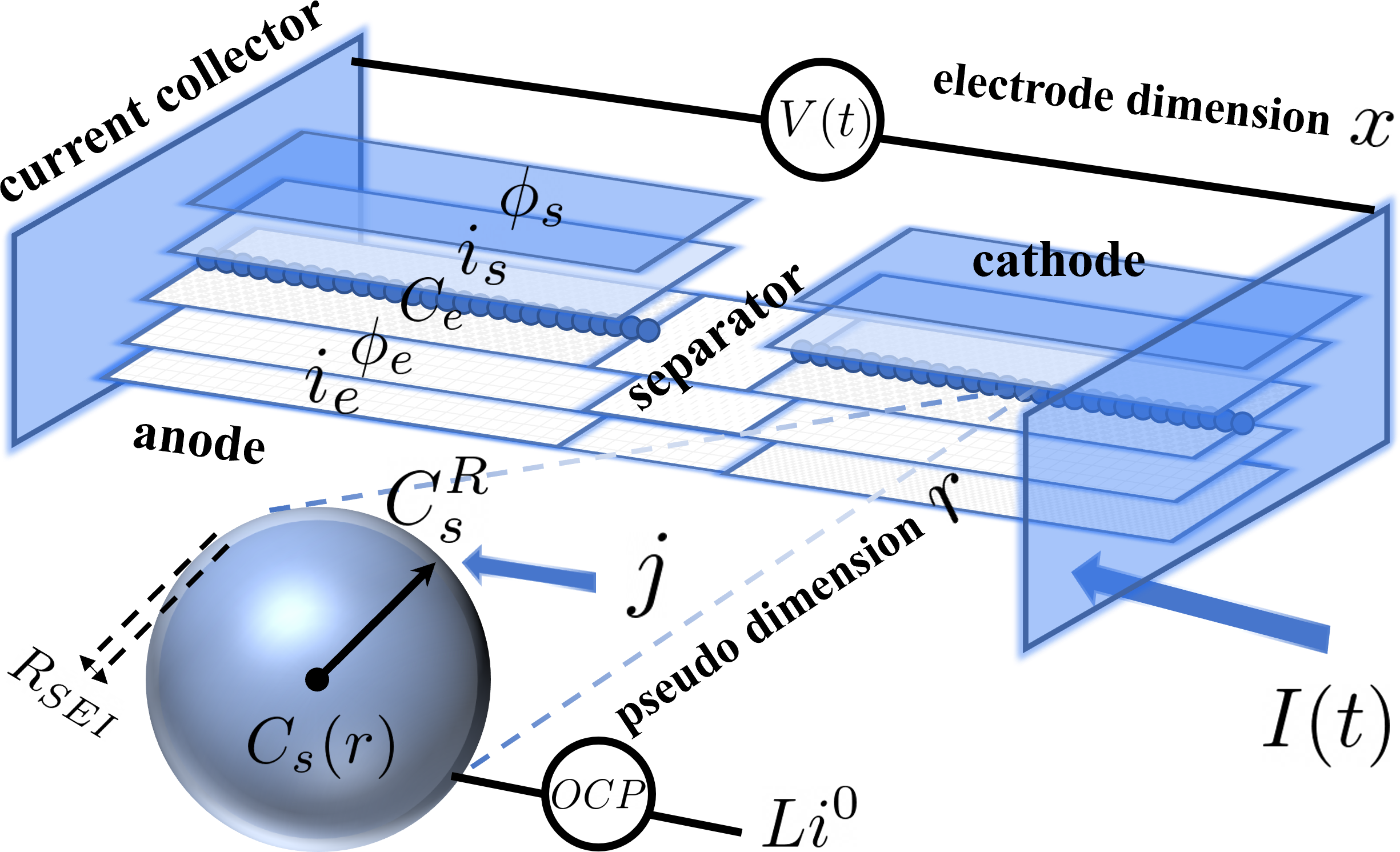
Figure 4: P2D representation of a LIB cell with superimposed continua spanning over two phases and three domains. The nomenclature can be found in the Supplementary Information.

To complete the P2D formulation, the electrolyte transport is modeled by a diffusion-reaction equation with a source term that couples it to the lithium-ion diffusion given by Eqn. (12) through the molar, interfacial flux $j$:

$$\epsilon_{e}\frac{\partial C_{e}}{\partial t}=\frac{\partial}{\partial x}\,\Bigg{(}D_{e}^{\text{eff}}\,\,\frac{\partial C_{e}}{\partial x}\Bigg{)}\,+\,a_{s}\,(1-t_{+}^{0})\,j,$$ (18)

where $\epsilon_{e}$, $a_{s}$, $D_{e}^{\text{eff}}$ and $t_{+}^{0}$ are the volume fraction and specific interfacial surface area of the active materials, the effective diffusion coefficient of the electrolyte and the transference number, respectively. The interfacial flux $j$ only exists in the anode and cathode domains and is zero otherwise.

3.2 MINN Battery Model

Eqns. (12)–(18) form a system of PDAEs, characterized by the circular, nested loops of algebraic variables $h_{z}(t)$, which couple the dynamical equations of the differential (dynamic) states $h_{d}(t)$ through the molar flux terms. The origin of these algebraic variables lies in the enormously different characteristic time scales of ionic and electron transport [38]. The resulting system is highly nonlinear and stiff, which poses challenges to numerical techniques. In order to employ specialized solvers optimized for accurate and stable time integration, the system is normally discretized in space, which results in a DAE system in its semi-explicit form,

$$\dot{h}_{d} =f\,\Big{(}h_{d},\,h_{z}\Big{)},$$ (19)

$$0 =g\,\Big{(}h_{d},\,h_{z},\,I(t)\Big{)},$$ (20)

where Eqn. (19) is an ODE system for ionic transport and Eqn. (20) are conservation laws resulting from (simplified) electron transport. The so-called hidden states are composed of differential states $h_{d}=[C_{s},\,C_{e}]^{T}$ and algebraic variables $h_{z}=j$. It is also required for the DAE solver to have a consistent initial condition $h(0)=[h_{d}^{0},\,h_{z}^{0}]^{T}$ that satisfies Eqn. (20). In the solution process of a DAE system, it must find roots of the algebraic system of equations $g\,(h_{d},\,h_{z},\,I)$ iteratively within solver tolerances because $h_{z}$ cannot be explicitly derived. In addition, the system is unstable at an occurrence when the system deviates from $g\,(h_{d},\,h_{z},\,I)=0$. In such an event, re-initialization is necessary through the discontinuous callback of the DAE solver whenever there is discontinuity detected in the input $I(t)$. Consequently, solving the DAE system originating from the P2D model becomes very expensive in the case of real-world driving cycles, which usually render the DAE solver prohibitively slow. To this end, the proposed MINN model circumvents the need for root finding as well as re-initialization.

The DAE system Eqns. (12)–(18) is of index one [7], which means that for $h_{d}$ at a given time $t$, Eqn. (18) defines $h_{z}$ uniquely. We can therefore find a locally unique solution $h^{*}_{z}$ for Eqn. (20). Accordingly, the DAE system can be written as one system of ordinary differential equations (ODEs),

$$\dot{h}_{d}=f\,\,\Big{(}\,h_{d},\,\,h^{*}_{z}\,\Big{)}.$$ (21)

The time integration of the ODE system (21) requires no re-initialization and computationally less workload. We then proceed to parameterize the function $G(h_{d},\,I)$ by a neural network whose size is dependent on the number of dynamic states (input) and algebraic variables (output). Consider approximating $G$ with a DNN of $L$ layers, i.e.,

$$\begin{cases}a^{[1]}=[h_{d},\,I]^{T}\in\mathbb{R}^{m}\\ a^{[l]}=\sigma\,\Big{(}W_{l}\,a^{[l-1]}\,+\,b_{l}\Big{)},\quad\text{for}\quad l=2,\,3,\,...,\,L\\ h^{*}_{z}=W_{L}a^{[L]}\,+\,b_{L}\in\mathbb{R}^{n}\end{cases}$$ (22)

Incidentally, the number of trainable parameters $\theta$ of this approximation $G_{\text{NN}}\,(h_{d},I;\theta)$ gets large when the order of the system $N=m+n$ is large, especially if the weight matrices $W_{l}$, biases $b_{l}$ and $L$ are also large. An orthogonal collocation method similar to [7] is used for spatial discretization of the PDAE system Eqns. (12)–(18) in this work to relieve the difficulty of training. For the same number of discretization points, this method is known to yield much smaller truncation errors than finite volume [12, 15], finite difference [39, 40] and finite element [41, 15] commonly used in battery modeling community, thanks to spectral accuracy.

There are $16$ boundary conditions in the P2D formulation that are necessary to describe the current and potential fields in three domains. This results in $16$ additional terms signifying the boundary loss in the loss function for a standard PINN setup, which is expensive and difficult to train. The convergence and regularisation of these terms also require additional hyperparameters for tuning. Unlike the physically constrained loss function in the PINN framework [28, 17], MINN accounts for the boundary conditions without specifying them explicitly in the loss function. Instead, they are imposed on the integration constants by considering, for example, the electrolyte potential $\phi_{e}$ as a function of the electrolyte current $i_{e}$ integrated over electrode dimension $x$, i.e.,

$$\phi_{e,i}=-\int\frac{i_{e,i}(x)}{\kappa_{\text{eff}}(x)}\,dx+A\,ln\,C_{e,i}\,(x)+B_{i}.$$ (23)

By substituting Eqn. (23) into the boundary conditions, three integration constants $B_{i}$ are obtained for each domain $i$, i.e., anode, separator and cathode. By the same token, the interfacial flux $j_{i}=\frac{1}{a_{s,i}F}\frac{\partial i_{e}}{\partial x}$ can be integrated as follows

$$i_{e,i}=a_{s,i}F\int j_{i}\,(x)\,dx+E_{i},$$ (24)

where the constants $E_{i}$ are fixed such that $i_{e}=0$ at the electrode-current collector interfaces and $i_{e}=I(t)$ at the electrode-separator interfaces. In this way, both $i_{e,i}$ and $\phi_{e,i}$ can be exclusively calculated from $j_{i}$, and so is $i_{s,i}$ because of Kirchhoff’s current law, $i_{s}\,+\,i_{e}\,=\,I(t)$. Eqn. (16) can also be integrated to yield two integration constants $\phi_{s,i}^{cc}$, which stand for the anode and cathode potentials at the current collector. This gives

$$\phi_{s,i}= \int-\frac{i_{s}(x)}{\sigma_{\text{eff}}}\,dx+\phi_{s,i}^{cc}$$ (25)

$$\phi_{s,i}^{cc}= \frac{2RT}{F}\sinh^{-1}\,\Bigg{(}\frac{j_{i}}{2i_{0}}\Bigg{)}+\phi_{e,i}$$

$$+\phi_{eq,i}-\phi_{s,i}+j_{i}\cdot R_{\text{SEI}}$$ (26)

$$Y_{V}= \phi_{s,a}^{cc}-\phi_{s,c}^{cc}.$$ (27)

Eqns. (23)–(25) reduce the algebraic variables to only the interfacial flux $j_{i}$ and $\phi_{s,i}^{cc}$. In turn, the algebraic system of equations amounts to

$$g=\begin{pmatrix}a_{s,a}F\int j_{a}(x)dx\\ a_{s,c}F\int j_{c}(x)dx\\ \int 2\,i_{0,a}\,\sinh\Big{(}\frac{F}{RT}\,\eta_{a}(x)\Big{)}\,dx\\ \int 2\,i_{0,c}\,\sinh\Big{(}\frac{F}{RT}\,\eta_{c}(x)\Big{)}\,dx\\ \end{pmatrix}+\begin{pmatrix}-1\\ 1\\ -1\\ 1\end{pmatrix}\cdot I(t)$$ (28)

The second term $\mathcal{L}_{y}$ in the loss function Eqn. (8) is the error in model outputs, and for a battery system, the experimental measurements can be the terminal voltage $Y_{V}$, SOC or lithium plating potential. The SOC of the battery system is defined by the average concentration of the anode particles over the electrode thickness $\delta$, normalized by the electrode stoichiometry at $100\%$ and $0\%$ SOC, and the plating potential is the difference between the solid and liquid potentials at the anode-separator interface (ASI), which give

$$Y_{\text{SOC}}\,(h_{d},h^{*}_{z},t)=\frac{3}{\delta\cdot R^{3}\,(C_{s}^{100\%}-C_{s}^{0\%})}$$

$$\qquad\quad\>\>\>\cdot\Bigg{(}\int^{\delta}_{0}\int^{R}_{0}\frac{r^{2}}{C_{s}^{\max}}\,C_{s}(x,r,t)\,dr\,dx\,-\,C_{s}^{0\%}\Bigg{)}$$ (29)

$$Y_{\text{plp}}\,(h_{d},h^{*}_{z},t)=\phi_{s}^{ASI}(t)\,-\,\phi_{e}^{ASI}(t).$$ (30)

4 Benchmarking and Training

This section introduces four state-of-the-art battery models for evaluating the performance of MINN, using physics-based, data-driven and hybrid approaches. First, we obtain the ground truth solutions using the P2D model. Second, we develop DNN and PINN battery models to learn the solution trajectories of the P2D model under a pre-defined control input. Lastly, to benchmark the learning of battery dynamics under time-varying control profiles, which could be unknown a priori, e.g., derived from real-time optimization or control, we develop a data-driven reduced-order model (DD-ROM).

4.1 P2D Battery Model

Newman’s P2D model serves as the ground truth for benchmarking. The model’s accuracy is dependent on the spatial discretization of the equations introduced in Section 3.1. To this end, we obtained a high-fidelity P2D model using the spectral Galerkin method consisting of 130 states and 14 algebraic variables. The resulting 144-order model is generated symbolically and the time integration is done using a legacy IDA solver [42].

4.2 Baseline DNN Battery Model

We generate a purely data-driven battery model using deep learning. A three-layer DNN with an input size equal to the number of states and output size equal to the dimension of the solution are parameterized. The DNN is then trained to map the initial condition of the discharge to the time trajectories of internal states $[h_{d}^{k},\,h_{z}^{k}]^{T}$ for a predefined current rate. The loss function is defined as

$$\mathcal{L}_{\text{DNN}}=\sum_{k=0}^{K}\,\Bigg{(}[\mathcal{NN}_{d}^{k},\,\mathcal{NN}_{z}^{k}]^{T}-[h_{d}^{k},\,h_{z}^{k}]^{T}\Bigg{)}^{2},$$ (31)

where $\mathcal{NN}_{d}^{k}$ and $\mathcal{NN}_{z}^{k}$ are the outputs of the DNN relating to the differential states and algebraic states at timestep $k$

4.3 PINN Battery Model

The PINN hybrid battery model is developed using the schemes illustrated in Fig. 1(b). In addition to the data-driven loss $\mathcal{L}_{\text{DNN}}$, the loss function for PINN includes a physical loss due to physical inconsistency:

$$\mathcal{L}_{\text{PINN}} =\mathcal{L}_{\text{DNN}}+\mathcal{L}_{\text{physical}},$$ (32)

$$\mathcal{L}_{\text{physical}} =\sum_{k=0}^{K}\,\Bigg{(}f\Big{(}\big{[}\mathcal{NN}_{d}^{k},\,\mathcal{NN}_{z}^{k}\big{]}^{T}\Big{)}-\frac{dh_{d}^{k}}{dt}\Bigg{)}^{2},$$ (33)

where $\frac{dh_{d}^{k}}{dt}$ is the time derivative of the differential states in the training data generated by the P2D model, and the function $f$ is the RHS of Eqn. (19), which embeds the dynamics of the P2D model.

4.4 DD-ROM Battery Model

Since baseline DNN and PINN only learn the solution trajectories for predefined $u(t)$, we develop an idealized battery model for the dynamic current input, assuming we have all the internal state data $[h_{d}^{k},h_{z}^{k}]^{T}$. In practice, the internal state measurements can be obtained by, e.g., using next-generation embedded sensors in laboratory settings. The training dataset for the data-driven-reduced order model (DD-ROM) consists of all internal state data with the corresponding labels, i.e., a pair of input-label data $X=[h_{d}^{k},\,I^{k}]^{T}$ and $Y=h_{z}^{k}$. The loss function for DD-ROM is defined by the mean square error (MSE) loss of the training data, in a supervised learning fashion. For $49$ pairs of input-label data taken from the high-order P2D solution, a mapping function $X\mapsto Y$ is parameterized by a DNN, and the loss is minimized down to machine zero using an optimizer. The downside of this hybrid scheme is that it depends on a vast amount of training data and has to include all battery internal states, which in many cases are not measurable but can only be obtained by physics-based models. Nevertheless, we train and present such a model with a never-before-seen current profile.

4.5 Training Details

The MINN model offers a new path to generating appropriate battery models by seamlessly blending the features of first-principle-based models with neural network architecture, which retrains the individual advantages of physics-based and data-driven approaches. Because certain neural network parameters $\theta$ may lead to unphysical states in Eqns. (4)-(7), we rectify the dynamic, algebraic and output functions $f$, $g$ and $Y$ by introducing rectified exponentials during training, e.g. the rectified square root, $\sqrt{x}\,_{\text{ReLU}}=\sqrt{\max(0,x)}$.

The DNN in the MINN architecture consists of three hidden layers with the same number of nodes as the other models. Forward mode automatic differentiation implemented in ForwardDiff.jl package in Julia [43] is adopted for the backpropagation. GELU activation function is used to mitigate training issues such as vanishing gradients usually associated with RNN [44]. All models in the benchmarks are trained with an ADAMW optimiser [45]. The learning rate is set to 0.001, and the training ends when the loss function flatlines. Generally, a wide-scale separation in the internal states and model output leads to the imbalance of loss function components. We scale the input-output data by characteristic time and internal state scales in order to approximate the widely separated scales in a single DNN.

5 Results and Discussion

This section evaluates the proposed MINN and compares it against the benchmarking models introduced in Section 4. The results of the comparative study are characterized by the model prediction accuracy, data efficiency, physical interpretability, and computational cost. It is worth noting that real-world battery applications could be complicated and in a wide range of usage conditions that may never be included in any training dataset. However, a reliable battery model must be able to generalize to out-of-sample usage profiles so that the levels of battery safety and degradation governed by physical states are not under- or overestimated. To test this critical ability of the referred models, we deliberately limit the range of conditions used to generate the training dataset.

5.1 Performance in learning solution trajectories

For a pre-defined control input, e.g. a constant discharge current, we design a scenario where the initial conditions of the testing data differ from that of the training data. Specifically, the developed DNN, PINN and MINN battery models are trained using P2D results generated by the first 250 seconds of a 1C discharge starting from 50% SOC. The testing data consists of the rest of the discharge together with a 1C discharge starting from 30% SOC. As shown in Fig. 5(e), for both the 50% and 30% SOC testing data, the DNN predictions of the battery terminal voltage diverge significantly from the P2D reference. For the internal states, e.g., electrolyte concentration and anode potential fields in Figs. 5(b) and (g), respectively, DNN gives completely unreliable results along both temporal and spatial coordinates. In addition, the outputs become unphysical, i.e., not a number (NaN), after 250 seconds due to the fractional exponents in the output function $Y(t,h_{d},h_{z},I)$. This is because the baseline DNN is model-agnostic and cannot accurately forecast the internal state trajectories under operational conditions that differ from the training data.

The PINN battery model can follow the discharge trajectory of the terminal voltage for the 50% SOC case because the training process of the model is informed of the P2D equations (as seen in Fig. 5(e)). However, it fails when the initial condition is altered to 30% SOC, as PINN does not account for the change in initial conditions. The locally distributed electrolyte concentration, solid-phase lithium ion concentration and anode potential resulting from PINN for the 30% SOC case also diverge from the P2D results. Notably, the low levels of electrolyte concentration marked by the orange isosurface in Fig. 5(c) appear to enlarge much later (after 250 seconds) and are also less spread-out in the anode. It is well known that electrolyte depletion may lead to safety risks such as lithium dendrite formation and pathological pathways in batteries’ aging trajectory [46]. Inaccurate predictions of electrolyte concentration will severely undermine the function of health-aware BMS. For example, the PINN battery model in Fig. 5(h) underestimates the anode potential in the 30% SOC case compared with the more accurate P2D result in Fig. 5(f). Similar errors can be found in other internal states, such as solid-phase concentrations (Supplementary Information), and will inevitably lead to underutilization of the battery capacity and energy. These internal state trajectories have important implications for battery health and safety diagnosis and must be accurately captured by the deployed model for next-generation BMS. The MINN battery model always faithfully captures all the local state and output information regardless of the initial SOC values, as illustrated by the spatiotemporal plots in Fig. 5(d) and (i), and the output trajectories in Fig. 5(e). This is attributed to the fact the MINN model learns the dynamics of the physical system instead of learning the solution trajectories of an autonomous system.

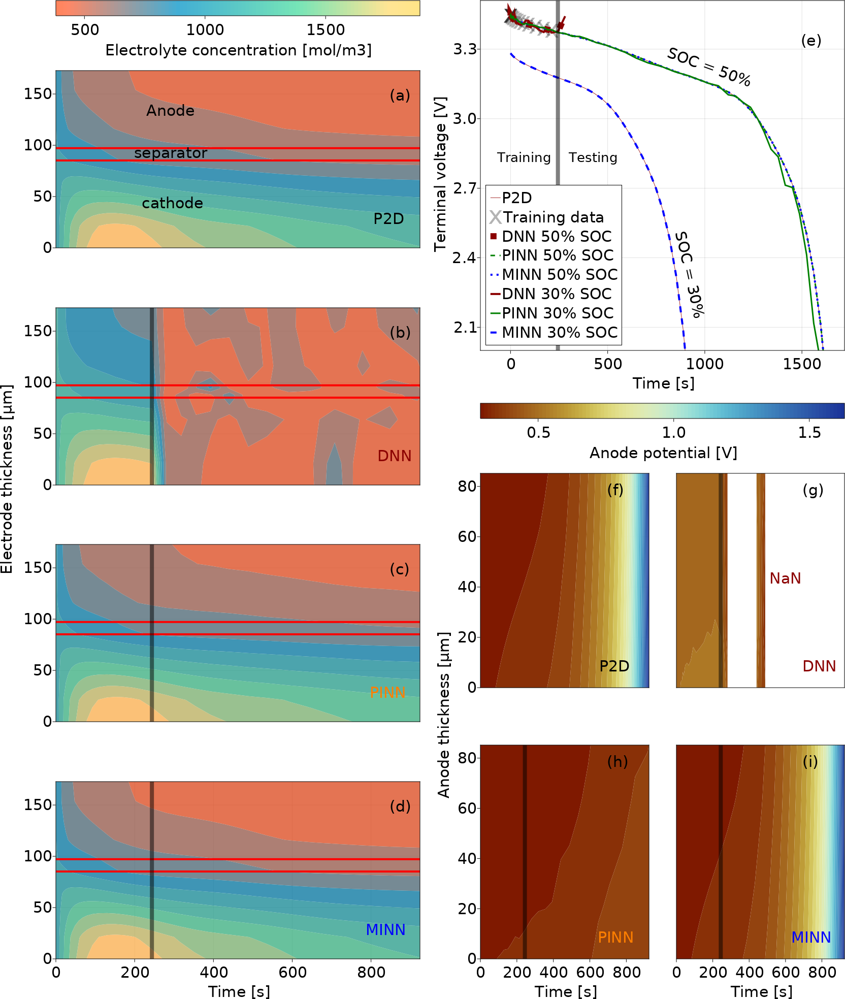
Figure 5: Comparison of different data-driven and hybrid models with P2D under 1C discharge. An LG M50 parameterization [47] is adopted in P2D to reproduce the dynamics of a battery faithfully and to generate internal battery state data for training. (a)-(d) Spatiotemporal plots of electrolyte concentration in the anode, separator and cathode for the discharge from SOC = 30%. (e) The terminal voltage curves of 1C discharge start from initial SOC values of 30% and 50%. (f)-(i) show the anode potential defined as $\phi_{s}-\phi_{e}$ for the discharge from SOC = 30%.

5.2 Performance in learning dynamics

To evaluate the effectiveness of hybrid models for learning battery dynamics, e.g., excited by prior unknown input profile, we use an arbitrary vehicle driving cycle to generate testing data. A challenging training dataset is purposefully chosen to evaluate MINN’s generalisability on unseen testing data. As shown in Fig. 6, the training dataset consists of 49 snapshots generated by the P2D model with the initial SOC fixed at $30\%$ and a sinusoidal input signal lasting only two seconds and bounded by 1C. By contrast, a highly dynamic current is used in the testing where the initial SOC is set to 90% and the maximum current reaches 5C.

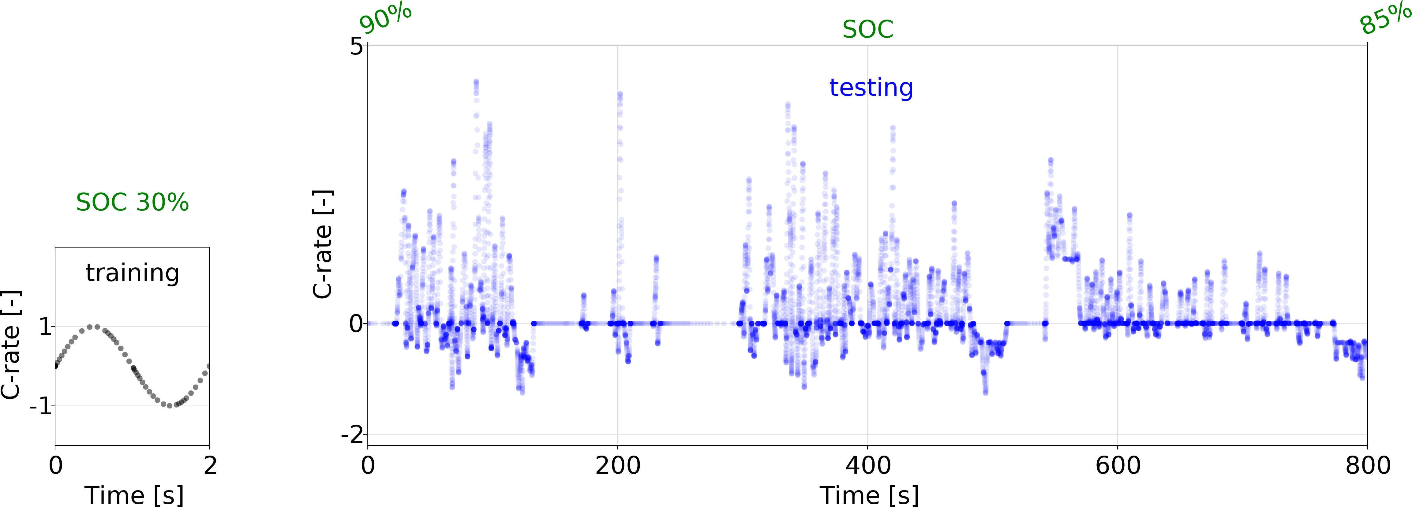
Figure 6: Dynamic current input profile and SOC range for generating training and testing dataset.

For an ideal case where all internal battery states are measurable, the DD-ROM is developed, whereby part of the model states are obtained by a relationship learnt from sampling the state trajectories of the P2D model. In comparison, the training of the MINN model involves only the experimentally measurable output of the P2D model, including the terminal voltage, lithium plating potential and SOC. Thanks to the built-in, problem-specific recurrent unit, it does not require the acquisition of the internal state data.

	Complexity				Training	generalization error
	System	Model order	Solver	Solution time [s] (mean)	Battery dataset	$\eta_{plp}$  [mV]	Voltage  [mV]	SOC  [%]
P2D	DAE	$130+14$	IDA (SUNDIALS)	$310.5$
DD-ROM	ODE	$130$	Rodas4	$3.4$	Internal states $h$	$9.88$	$9.87$	$0.635$
MINN	ODE	$82$	Rodas4	$1.7$	Measurement $Y$	$6.28$	$11.6$	$0.059$

TABLE I: Model complexity, data efficiency in training and the generalization error of DD-ROM and MINN battery models are compared with results of a dynamic driving profile obtained by a high-fidelity P2D model with the LG M50 parameterization (see Supplementary Information: parameterization). The generalization error is measured in root mean square error (RMSE) against the P2D benchmark. The solver used for the DAE system representing the 144-order P2D model is a legacy SUNDIALS solver [42], and the solver for ODE systems uses a 4th-order A-stable stiffly stable Rosenbrock method. All models are implemented using the DifferentialEquations.jl package in Julia [48].

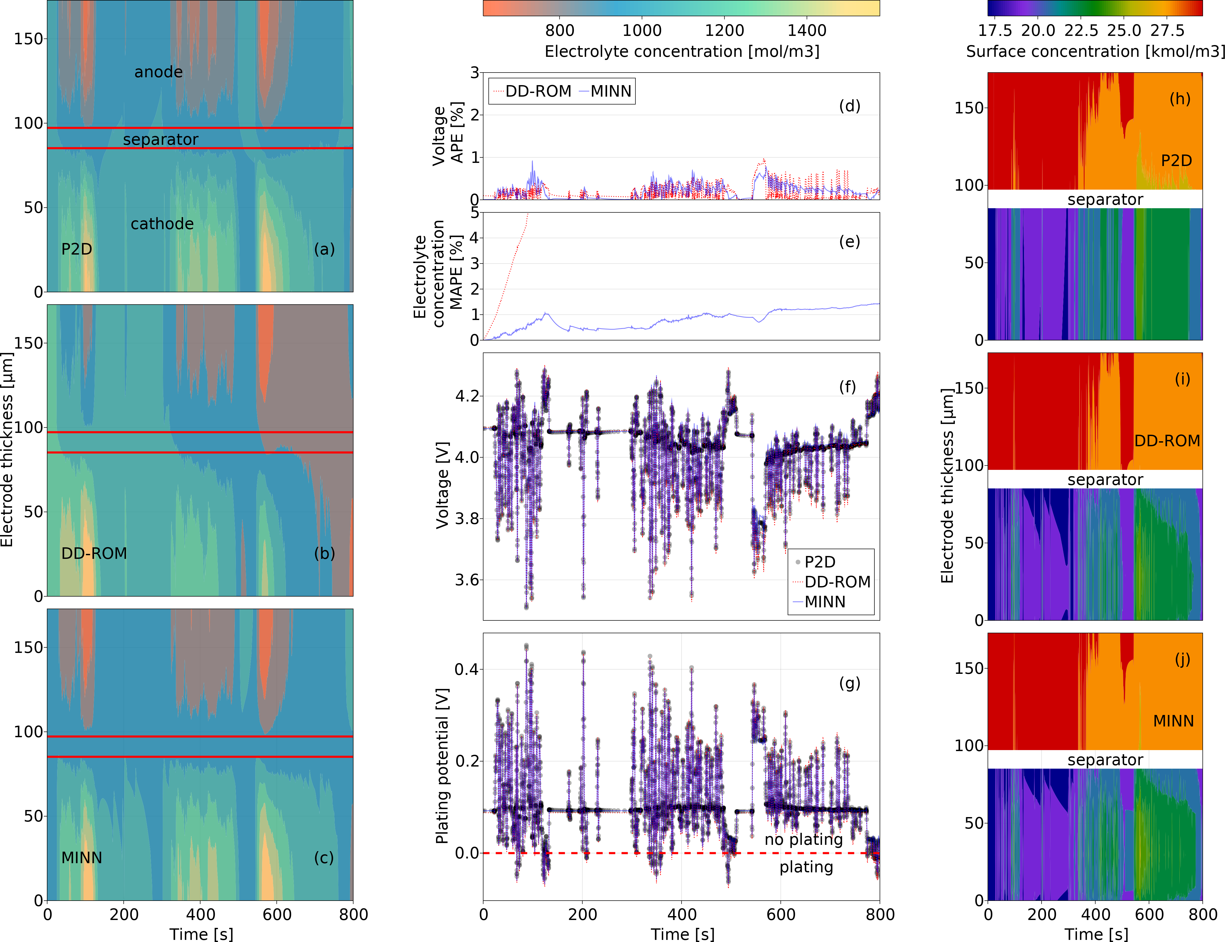
Figure 7: Performance of the DD-ROM and MINN battery models in learning system dynamics, compared with the results of reference 144-order P2D model. (a)-(c) Liquid-phase ion concentration (electrolyte concentration). (d)-(e) generalization errors of terminal voltage and electrolyte concentration. (f) Terminal voltage response to the testing current. (g) Anode plating potential at the anode-separator interface. (h)-(j) Solid-phase concentration at the surface of particles.

Accurate prediction of the system outputs, including the terminal voltage, plating potential and SOC, is important to advance BMS functionalities, such as power capability prediction [49] and health-aware fast charging [10, 50]. Table I shows the computational complexity, training dataset and numerical accuracy of the above three battery models in predicting these outputs, while Fig. 7(g) displays the trajectory of the plating potential. Both the MINN and DD-ROM models show high accuracy in the terminal voltage, achieving generalization errors of less than 12 mV. In Fig. 7(g), the red dashed line at $0$ V highlights the critical level below which the lithium plating is triggered. To predict such plating potential, the MINN model is as good as the DD-ROM which is developed under the hypothetically available information of all battery states. Regarding SOC prediction, the MINN model has greater accuracy than the DD-ROM, with a generalization error of only 0.06%. Other testing data generated at various initial conditions other than 85%-90% SOC have also been considered, which has yielded similar results in predicting the model outputs and further confirmed the superiority of MINN over DD-ROM. This achievement by MINN with only the measurement data for training is practical during real-world battery usage. In fact, the upper limit of the accuracy of MINN is not the first-principle model used in this benchmark but the battery system itself.

To evaluate MINN’s capability of predicting the dynamics of internal battery states, the locally distributed electrolyte concentration and solid-phase surface concentration are examined in spatiotemporal plots. As shown in Fig. 7(c), MINN is capable of reproducing the electrolyte evolution accurately along the challenging operating profile with a mean absolute percentage error (MAPE) plotted in Fig. 7(e) of less than 2%. Although DD-ROM battery model gives less than 1% absolute percentage error (APE) for the terminal voltage as shown in Fig. 7(d), it under- and overestimates the degree of electrolyte depletion. For example, at around 100 seconds, marked by a blue isosurface, the DD-ROM model underestimates the depletion in the anode and yet overestimates it in the anode, separator and cathode starting from 600 seconds (light orange). Fig. 7(h–j) depicts the comparative results for the solid-phase concentration. Here, the colour red represents the theoretical maximum surface concentration of graphite particles, near which the movement of lithium ions matches the intercalation threshold of lattice sites in the anode and the dendritic growth of lithium is inevitable [51]. The DD-ROM prediction in Fig. 7(i) yields larger red areas adjacent to the anode-separator interface, which means significantly more lithium plating if one deploys it in the BMS. In addition, DD-ROM overestimates the surface concentration in the anode at 500 seconds. When imposing a constraint on the surface concentration for vehicle battery control, such overestimation will curtail the energy recovered from regenerative braking [52]. However, the MINN predicts the critical surface concentration in Fig. 7(j) as close as the P2D during the entire process, thereby allowing accurate monitoring and control of the solid-phase concentration.

5.3 Computational costs

Next, the computational costs of DD-ROM and MINN are examined alongside the P2D model. In practice, most P2D model implementations feature additional algebraic state variables that are converged at each time step by using, e.g. an iterative algorithm. While these implementations may realize millisecond-scale simulations [14] for static charge and discharge, the solution time can be prohibitively slow for dynamic driving profiles due to increasing stiffness. As shown in Table I, the hybrid models achieve two orders of magnitude speedup in the solution time for an 800-second vehicle driving test, of which the MINN battery model has a slight edge over the DD-ROM model. The significant speed improvement of the MINN framework compared to DD-ROM is attributed to its high data efficiency, which allows for learning the complex dynamics of batteries without the need for a fixed number of internal states. This unique feature enables low-order approximations, as demonstrated by developing an 82-order model in Table I, in contrast to DD-ROM, which requires 130 states for similar accuracy. The remarkable speedup in computational time will make it possible onboard model-based applications, such as online parameter identification, state estimation and closed-loop control. Indeed, a vast majority of daily battery usage is driven by time-varying current profiles, under which the identifiability of battery models, including the P2D and MINN, will often be improved significantly compared to static excitations. Therefore, improving computational efficiency under dynamic operating conditions will help lift the computational burden of parameterization.

5.4 Discussion on adaptive battery modeling

During battery lifetime, conventional physics-based modeling requires periodic re-parameterization because of the ever-changing nature of multi-physical battery parameters due to ageing [53, 54]. The need for computationally expensive re-parameterization undermines the applications of physics-based models, which are supposed to have minimal dependence on data acquisition and training. This is evidenced by the fact that no mass-produced BMS on the market today has claimed the usage of physics-based models. MINN allows for the simplification of DAE structure and may potentially improve the identifiability of parameters. Accordingly, MINN can be used for aging adaptive models for a wide range of intelligent battery management applications, not only in the short term of several hours or days but also over the battery’s entire lifespan. Numerous examples of such applications include fast charging, lifetime optimization, thermal fault detection, and safety prognosis, which are the main challenges of BMS algorithm design.

6 Conclusion

The rapid upscaling of battery-powered electric vehicles makes it possible to collect big data. Based on the data, a wave of data-driven models under the hood of machine learning has recently been developed in the battery community. While data-driven surrogate models excel in learning complex battery characteristics, they inherently lack the ability to generalize beyond the training data and provide a physical interpretation of the internal battery status. With the potential to combine the merits of physics-based and data-driven models, we propose a conceptually novel neural network architecture, MINN, for hybrid modeling. It has been shown to be accurate in output and internal state predictions while achieving remarkable acceleration in the solution time. The MINN battery model is data-efficient to train compared with DD-ROM. Its built-in physical parameters and interpretable hidden states are important in battery system identification, fault diagnostics, safety prognostics, and physics-based control. The substantial and practical benefits offered by MINN make it an exceptional choice for developing the next-generation BMS. By integrating machine learning with physics-based modeling, the MINN framework offers a powerful tool for analyzing general dynamic systems commonly found in diverse fields, such as mechatronics, thermal fluid dynamics, electrical power systems, and energy storage systems.

References

- Liang and Yao [2018] Y. Liang and Y. Yao, “Positioning organic electrode materials in the battery landscape,” Joule, 2018.
- Jin et al. [2018] Y. Jin, K. Liu, J. Lang, D. Zhuo, Z. Huang, C.-A. Wang, H. Wu, and Y. Cui, “An intermediate temperature garnet-type solid electrolyte-based molten lithium battery for grid energy storage,” Nature Energy, vol. 3, pp. 732–738, 2018.
- Farmann and Sauer [2018] A. Farmann and D. U. Sauer, “Comparative study of reduced order equivalent circuit models for on-board state-of-available-power prediction of lithium-ion batteries in electric vehicles,” Appl. Energy, 2018.
- Li et al. [2020] W. Li, D. Cao, D. Jöst, F. Ringbeck, M. Kuipers, F. Frie, and D. U. Sauer, “Parameter sensitivity analysis of electrochemical model-based battery management systems for lithium-ion batteries,” Appl. Energy, vol. 269, p. 115104, 2020.
- Khalik et al. [2021] Z. Khalik, M. Donkers, J. Sturm, and H. Bergveld, “Parameter estimation of the Doyle-Fuller-Newman model for lithium-ion batteries by parameter normalization, grouping, and sensitivity analysis,” J. Power Sources, vol. 499, p. 229901, 2021.
- Zou et al. [2016a] C. Zou, C. Manzie, D. Nešić, and A. G. Kallapur, “Multi-time-scale observer design for state-of-charge and state-of-health of a lithium-ion battery,” J. Power Sources, vol. 335, pp. 121–130, 2016.
- Bizeray et al. [2015] A. Bizeray, S. Zhao, S. Duncan, and D. Howey, “Lithium-ion battery thermal-electrochemical model-based state estimation using orthogonal collocation and a modified extended Kalman filter,” J. Power Sources, vol. 296, pp. 400–412, 2015.
- Yang et al. [2017] X.-G. Yang, Y. Leng, G. Zhang, S. Ge, and C.-Y. Wang, “Modeling of lithium plating induced aging of lithium-ion batteries: Transition from linear to nonlinear aging,” J. Power Sources, vol. 360, pp. 28–40, 2017.
- Jones et al. [2022] P. K. Jones, U. Stimming, and A. A. Lee, “Impedance-based forecasting of lithium-ion battery performance amid uneven usage,” Nat. Commun., vol. 13, no. 1, Aug. 2022.
- Zou et al. [2018] C. Zou, C. Manzie, and D. Nesic, “Model predictive control for lithium-ion battery optimal charging,” IEEE/ASME Trans. Mechatronics, vol. 23, no. 2, pp. 947–957, 2018.
- Kolluri et al. [2020] S. Kolluri, S. V. Aduru, M. Pathak, R. D. Braatz, and V. R. Subramanian, “Real-time nonlinear model predictive control (NMPC) strategies using physics-based models for advanced lithium-ion battery management system (BMS),” J. Electrochem. Soc., vol. 167, no. 6, p. 063505, 2020.
- Torchio et al. [2016] M. Torchio, L. Magni, R. B. Gopaluni, R. D. Braatz, and D. M. Raimondo, “LIONSIMBA: A Matlab framework based on a finite volume model suitable for Li-ion battery design, simulation, and control,” J. Electrochem. Soc., vol. 163, no. 7, pp. A1192–A1205, 2016.
- Han et al. [2021] S. Han, Y. Tang, and S. K. Rahimian, “A numerically efficient method of solving the full-order pseudo-2-dimensional (P2D) Li-ion cell model,” J. Power Sources, vol. 490, p. 229571, 2021.
- Berliner et al. [2021] M. D. Berliner, H. Zhao, S. Das, M. Forsuelo, B. Jiang, W. H. Chueh, M. Z. Bazant, and R. D. Braatz, “Nonlinear identifiability analysis of the porous electrode theory model of lithium-ion batteries,” J. Electrochem. Soc., vol. 168, no. 9, p. 090546, 2021.
- Sulzer et al. [2021] V. Sulzer, S. G. Marquis, R. Timms, M. Robinson, and S. J. Chapman, “Python Battery Mathematical Modelling (PyBaMM),” J. Open Res. Softw, vol. 9, no. 1, p. 14, 2021.
- Korotkin et al. [2021] I. Korotkin, S. Sahu, S. E. J. O'Kane, G. Richardson, and J. M. Foster, “DandeLiion v1: An extremely fast solver for the Newman model of lithium-ion battery (dis)charge,” J. Electrochem. Soc., 2021.
- Raissi et al. [2017a] M. Raissi, P. Perdikaris, and G. E. Karniadakis, “Physics informed deep learning (Part II): Data-driven discovery of nonlinear partial differential equations,” ArXiv, 2017.
- Chaturvedi et al. [2010] N. A. Chaturvedi, R. Klein, J. Christensen, J. Ahmed, and A. Kojic, “Algorithms for advanced battery-management systems,” IEEE Control Systems, vol. 30, pp. 49–68, 2010.
- Li et al. [2019] Y. Li, M. Vilathgamuwa, T. W. Farrell, S. S. Choi, N. T. Tran, and J. Teague, “A physics-based distributed-parameter equivalent circuit model for lithium-ion batteries,” Electrochim. Acta, 2019.
- Li et al. [2021] Y. Li, D. M. Vilathgamuwa, E. Wikner, Z. Wei, X. Zhang, T. Thiringer, T. Wik, and C. Zou, “Electrochemical model-based fast charging: Physical constraint-triggered PI control,” IEEE Trans. Energy Convers., vol. 36, no. 4, pp. 3208–3220, 2021.
- Aitio and Howey [2021] A. Aitio and D. A. Howey, “Predicting battery end of life from solar off-grid system field data using machine learning,” Joule, 2021.
- Hu et al. [2020] X. Hu, L. Xu, X. Lin, and M. G. Pecht, “Battery lifetime prognostics,” Joule, 2020.
- Chen et al. [2022] B.-R. Chen, C. Walker, S. Kim, M. R. Kunz, T. R. Tanim, and E. J. Dufek, “Battery aging mode identification across nmc compositions and designs using machine learning,” Joule, 2022.
- Liu et al. [2021] Y. Liu, X. Shu, H. Yu, J. Shen, Y. Zhang, Y. Liu, and Z. Chen, “State of charge prediction framework for lithium-ion batteries incorporating long short-term memory network and transfer learning,” J. Energy Storage, vol. 37, p. 102494, 2021.
- Harris et al. [2009] S. J. Harris, A. T. Timmons, D. R. Baker, and C. W. Monroe, “Direct in situ measurements of Li transport in Li-ion battery negative electrodes,” Chem. Phys. Lett., vol. 485, pp. 265–274, 2009.
- Wang et al. [2020] H. Wang, Y. Zhu, S. C. Kim, A. Pei, Y. Li, D. T. Boyle, H. Wang, Z. Zhang, Y. Ye, W. Huang, Y. Liu, J. Xu, J. Li, F. Liu, and Y. Cui, “Underpotential lithium plating on graphite anodes caused by temperature heterogeneity,” Proc. Natl. Acad. Sci., vol. 117, pp. 29 453 – 29 461, 2020.
- Gao et al. [2021] T. Gao, Y. Han, D. Fraggedakis, S. Das, T. Zhou, C.-N. Yeh, S. Xu, W. C. Chueh, J. Li, and M. Z. Bazant, “Interplay of lithium intercalation and plating on a single graphite particle,” Joule, 2021.
- Raissi et al. [2017b] M. Raissi, P. Perdikaris, and G. E. Karniadakis, “Physics informed deep learning (Part I): Data-driven solutions of nonlinear partial differential equations,” ArXiv, 2017.
- Raissi et al. [2018] ——, “Multistep neural networks for data-driven discovery of nonlinear dynamical systems,” ArXiv: Dynamical Systems, 2018.
- Lu et al. [2020] L. Lu, X. Meng, Z. Mao, and G. E. Karniadakis, “Deepxde: A deep learning library for solving differential equations,” SIAM Rev., vol. 63, pp. 208–228, 2020.
- Hennigh et al. [2021] O. Hennigh, S. Narasimhan, M. A. Nabian, A. Subramaniam, K. M. Tangsali, M. Rietmann, J. del Águila Ferrandis, W. Byeon, Z. Fang, and S. Choudhry, “Nvidia simnet: an AI-accelerated multi-physics simulation framework,” in ICCS, 2021.
- Zubov et al. [2021] K. Zubov, Z. McCarthy, Y. Ma, F. Calisto, V. Pagliarino, S. Azeglio, L. Bottero, E. Luján, V. Sulzer, A. Bharambe et al., “NeuralPDE: Automating physics-informed neural networks (PINNs) with error approximations,” arXiv, 2021.
- Krishnapriyan et al. [2021] A. S. Krishnapriyan, A. Gholami, S. Zhe, R. M. Kirby, and M. W. Mahoney, “Characterizing possible failure modes in physics-informed neural networks,” in NeurIPS, 2021.
- Chen et al. [2018] T. Q. Chen, Y. Rubanova, J. Bettencourt, and D. K. Duvenaud, “Neural ordinary differential equations,” in NeurIPS, 2018.
- Doyle et al. [1993] M. Doyle, T. F. Fuller, and J. Newman, “Modeling of galvanostatic charge and discharge of the lithium/polymer/insertion cell,” J. Electrochem. Soc., vol. 140, no. 6, pp. 1526–1533, 1993.
- Fuller et al. [1994] T. F. Fuller, M. L. Doyle, and J. Newman, “Simulation and optimization of the dual lithium ion insertion cell,” J. Electrochem. Soc., vol. 141, pp. 1–10, 1994.
- Newman and Thomas-Alyea [2012] J. Newman and K. E. Thomas-Alyea, Electrochemical systems. John Wiley & Sons, 2012.
- Zou et al. [2016b] C. Zou, C. Manzie, and D. Nesic, “A framework for simplification of PDE-Based lithium-ion battery models,” IEEE Trans. Contr. Syst. Technol., vol. 24, pp. 1594–1609, 2016.
- Newman [1998] J. Newman, “Fortran programs for simulation of electrochemical systems: Dualfoil,” http://www.cchem.berkeley.edu/jsngrp/fortran.html, 1998.
- Moura [2016] S. J. Moura, “Fast Doyle-Fuller-Newman (DFN) electrochemical-thermal battery model simulator,” https://github.com/scott-moura/fastDFN, 2016.
- Cai and White [2011] L. Cai and R. E. White, “Mathematical modeling of a lithium ion battery with thermal effects in COMSOL Inc. Multiphysics (MP),” J. Power Sources, vol. 196, no. 14, pp. 5985–5989, 2011.
- Hindmarsh et al. [2005] A. C. Hindmarsh, P. N. Brown, K. E. Grant, S. L. Lee, R. Serban, D. E. Shumaker, and C. S. Woodward, “Sundials: Suite of nonlinear and differential/algebraic equation solvers,” ACM Trans. Math. Softw., vol. 31, no. 3, p. 363–396, 2005.
- Revels et al. [2016] J. Revels, M. Lubin, and T. Papamarkou, “Forward-mode automatic differentiation in Julia,” arXiv, 2016.
- Hendrycks and Gimpel [2016] D. Hendrycks and K. Gimpel, “Gaussian error linear units (GELUs),” arXiv: Learning, 2016.
- Loshchilov and Hutter [2017] I. Loshchilov and F. Hutter, “Decoupled weight decay regularization,” ICLR, 2017.
- Attia et al. [2022] P. M. Attia, A. Bills, F. B. Planella, P. Dechent, G. dos Reis, M. Dubarry, P. Gasper, R. Gilchrist, S. Greenbank, D. A. Howey, O. Liu, E. Khoo, Y. Preger, A. S. Soni, S. Sripad, A. G. Stefanopoulou, and V. Sulzer, “Review—"knees" in lithium-ion battery aging trajectories,” J. Electrochem. Soc., 2022.
- Chen et al. [2020] C.-H. Chen, F. B. Planella, K. B. O’Regan, D. Gastol, W. D. Widanage, and E. Kendrick, “Development of experimental techniques for parameterization of multi-scale lithium-ion battery models,” J. Electrochem. Soc., 2020.
- Rackauckas and Nie [2017] C. Rackauckas and Q. Nie, “Differentialequations.jl – a performant and feature-rich ecosystem for solving differential equations in julia,” J. Open Res. Softw, vol. 5, p. 15, 2017.
- Wik et al. [2015] T. Wik, B. Fridholm, and H. Kuusisto, “Implementation and robustness of an analytically based battery state of power,” J. Power Sources, vol. 287, pp. 448–457, 2015.
- Sieg et al. [2019] J. Sieg, J. Bandlow, T. Mitsch, D. Dragicevic, T. Materna, B. Spier, H. Witzenhausen, M. Ecker, and D. U. Sauer, “Fast charging of an electric vehicle lithium-ion battery at the limit of the lithium deposition process,” J. Power Sources, vol. 427, pp. 260–270, 2019.
- Guo et al. [2015] Z. Guo, J. Zhu, J. Feng, and S. Du, “Direct in situ observation and explanation of lithium dendrite of commercial graphite electrodes,” RSC Advances, vol. 5, pp. 69 514–69 521, 2015.
- Wikander et al. [2019] L. Wikander, B. Fridholm, S. Gros, and T. Wik, “Ideal benefits of exceeding fixed voltage limits on lithium-ion batteries with increasing cycle age,” J. Power Sources, 2019.
- Streb et al. [2022] M. Streb, M. Ohrelius, M. Klett, and G. Lindbergh, “Improving li-ion battery parameter estimation by global optimal experiment design,” J. Energy Storage, 2022.
- Streb et al. [2023] M. Streb, M. Andersson, V. L. Klass, M. Klett, M. Johansson, and G. Lindbergh, “Investigating re-parametrization of electrochemical model-based battery management using real-world driving data,” eTransportation, 2023.