On the capacity of a quantum perceptron for storing biased patterns

Abstract

Although different architectures of quantum perceptrons have been recently put forward, the capabilities of such quantum devices versus their classical counterparts remain debated. Here, we consider random patterns and targets independently distributed with biased probabilities and investigate the storage capacity of a continuous quantum perceptron model that admits a classical limit, thus facilitating the comparison of performances. Such a more general context extends a previous study of the quantum storage capacity where using statistical mechanics techniques in the limit of a large number of inputs, it was proved that no quantum advantages are to be expected concerning the storage properties. This outcome is due to the fuzziness inevitably introduced by the intrinsic stochasticity of quantum devices. We strengthen such an indication by showing that the possibility of indefinitely enhancing the storage capacity for highly correlated patterns, as it occurs in a classical setting, is instead prevented at the quantum level.

Keywords: quantum perceptron, storage capacity, quantum neural networks

1 Introduction

Machine learning aims at building methods that are able to make predictions or decisions based on sample data, without being explicitly programmed to do so. Quantum information theory studies the storage and transmission of information encoded in quantum states. Nowadays these two disciplines are becoming intertwined giving rise to the field of quantum machine learning.

The flow of ideas runs both ways: on the one hand applications of machine learning techniques are envisaged to analyze quantum systems [1, 2], on the other hand, the implementation of machine learning concepts on quantum hardware is also actively investigated [3, 4, 5]. Along this latter avenue quantum advantages are expected in terms of higher storage capabilities and an increased information processing power [6, 7, 8, 9].

The task of precisely comparing the power of quantum and classical neural networks as probabilistic models for information processing and storage is thus becoming pressing. In particular, the issue of determining precisely the storage capacity of the most elementary constituent of a neural network, namely the perceptron [10], has been addressed in the classical scenario without referring to any specific learning rule using several approaches, ranging from combinatorics [11, 12] to statistical mechanics methods [13, 14, 15, 16]. The latter has been used recently to generalize the calculation to some models of quantum perceptrons [17, 18, 19]. However, the results depend on the specific model used (see e.g. [18] and [19], based respectively on the models [5] and [20]).

Here, by referring to the continuous variable quantum perceptron model introduced in [20], we study the storage capacity of random classical binary patterns. The components of the patterns and their assigned output classification are taken to be independent and identically distributed (i.i.d.) according to a probability with a bias $-1\leq m_{\mathrm{in}}\leq 1$ for the patterns and $-1\leq m_{\mathrm{out}}\leq 1$ for their classification. Such a model admits the classical perceptron as a classical limit, thus enabling a direct comparison of the storage performances in the two cases. For classical perceptrons, simultaneously large biases for patterns and output classification allow to greatly enhance the storage capacity, which diverges when $m_{\mathrm{in}}=m_{\mathrm{out}}=m\to 1$ [13, 21, 22, 23]. We show that this possibility is prevented at the quantum level. Moreover, we also find that, when the biases $m_{\mathrm{in}}$ and $m_{\mathrm{out}}$ are varied separately, the quantum storage capacity depends on both of them, unlike in the classical case, where the storage capacity is a function only of the output bias. However, also in the quantum setting, when the output correlations are maximal, that is when $m_{\mathrm{out}}\to 1$, the asymptotic behaviour is no more dependent on $m_{\mathrm{in}}$, exactly as in the classical case. The dependence of the quantum storage capacity on $m_{\mathrm{in}}$ in such a case is through the velocity with which the limit behaviour is reached. Overall, the performances of the continuous quantum model remain below the classical ones. These results thus corroborate those found in Ref.[19] with unbiased patterns. They confirm that, at the level of a simple, that is one-layer, quantum perceptron, the uncertainties brought about by pattern encoding via Gaussian states and homodyne measurements cannot be counteracted by linear super-positions of pattern states.

2 A continuous quantum perceptron model

The continuous variable model of a quantum perceptron proposed in Ref.[20] is characterized by $N$ bosonic input modes and one bosonic output mode. The components $x_{j}$ of an input pattern $\boldsymbol{x}\in\mathbb{R}^{N}$ are encoded by states of the form

$$|\psi_{j}\rangle=\frac{1}{(2\pi\sigma^{2}_{j})^{1/4}}\int_{-\infty}^{+\infty}\mathrm{d}q_{j}\ {\exp\left(-\frac{(q_{j}-x_{j})^{2}}{4\sigma^{2}_{j}}\right)}|q_{j}\rangle,$$ (1)

which are Gaussian weighted normalized super-positions of pseudo-eigenstates $|q_{j}\rangle$ of position-like operators $q_{j}$, centered around the pattern components $x_{j}$ with widths $\sigma_{j}$. As a result, a pattern $\boldsymbol{x}$ is encoded into

$$|\Psi\rangle=\bigotimes_{j=1}^{N}|\psi_{j}\rangle.$$ (2)

Such a state is then given as input to a quantum circuit which first operates with a series of independent squeezing operators

$$S_{j}(r_{j})=\mathrm{e}^{\mathrm{i}\,r_{j}\,(q_{j}p_{j}+p_{j}q_{j})}\ ,\quad r_{j}\in\mathbb{R}\ ,\quad{\rm e}^{-2r_{j}}=w_{j}\ ,$$ (3)

where $p_{j}$ is a momentum-like operator conjugated to $q_{j}$ ($[q_{j},p_{j}]=\mathrm{i}$) and $r_{j}$ is the squeezing parameter implementing the weight $w_{j}$. Notice that

$$S_{j}(r_{j})|q_{j}\rangle=\sqrt{w_{j}}\,|w_{j}q_{j}\rangle\ .$$ (4)

Then, the circuit consists of entangling Controlled Addition gates $\mathrm{CX}$ on pairs of consecutive modes:

$${\mathrm{CX}_{j,j+1}}:=\exp\left(-\mathrm{i}\,q_{j}\otimes p_{j+1}\right)\ ,\qquad{\mathrm{CX}_{j,j+1}}\,|q_{j},q_{j+1}\rangle=|q_{j},q_{j}+q_{j+1}\rangle\ .$$ (5)

Their combined action on the attenuated multi-mode position eigenstates gives

$$\begin{split}|w_{1}q_{1},w_{2}q_{2},\ldots,w_{N}q_{N}\rangle&\rightarrow|w_{1}q_{1},w_{1}q_{1}+w_{2}q_{2},\ldots,w_{N}q_{N}\rangle\rightarrow\ldots\\ &\ldots\rightarrow|w_{1}q_{1},w_{1}q_{1}+w_{2}q_{2},\ldots,\sum_{j=1}^{N}w_{j}q_{j}\rangle\ .\end{split}$$ (6)

In such a way, the amplitude associated to the last mode position eigenstate has the form of a Gaussian distribution centered around $\boldsymbol{w}\cdot\boldsymbol{x}^{\mu}=\sum_{j=1}^{N}w_{j}x^{\mu}_{j}$:

$$\psi_{\boldsymbol{w},\boldsymbol{x}^{\mu}}(s)=\frac{1}{(2\pi\|\boldsymbol{w}\|^{2}\,\sigma^{2})^{1/4}}\exp\left(-\frac{(s-\boldsymbol{w}\cdot\boldsymbol{x}^{\mu})^{2}}{4\|\boldsymbol{w}\|^{2}\,\sigma^{2}}\right),\quad\|\boldsymbol{w}\|^{2}=\sum_{j=1}^{N}w^{2}_{j}\ ,$$ (7)

where, for sake of simplicity, we have set $\sigma_{j}^{2}=\sigma^{2}$ for all $j$ and thus encoded the input patterns by Gaussian states of the same width. Finally, homodyne detection operated on the last mode position-like quadrature yields a value $s$ with probability density

$$P_{\boldsymbol{w},\boldsymbol{x}^{\mu},\sigma}(s)=|\psi_{\boldsymbol{w},\boldsymbol{x}^{\mu}}(s)|^{2}=\frac{1}{\sqrt{2\pi}\|\boldsymbol{w}\|\sigma}\exp\left(-\frac{(s-\boldsymbol{w}\cdot\boldsymbol{x}^{\mu})^{2}}{2\|\boldsymbol{w}\|^{2}\sigma^{2}}\right).$$ (8)

Remark 1

With a slight modification of the above protocol, it is possible to obtain a description of such a continuous variable quantum perceptron as controlled unitary acting on the tensor product $\mathscr{H}=\mathscr{H}_{\mathrm{in}}\otimes\mathscr{H}_{\mathrm{out}}$ where $\mathscr{H}_{\mathrm{in}}$ is the Hilbert space of the $N$ bosonic modes encoding the input, while $\mathscr{H}_{\mathrm{out}}$ is the Hilbert space of the additional ancilla mode storing the output. Then, the present model can be connected with other models investigated in the literature, in particular [24], where it was pointed out that a perceptron acting as a controlled unitary has as particular cases also the models considered in [25, 26]. Actually, the action of the continuous variable quantum perceptron here investigated can be described with the unitary

$$U(\boldsymbol{w}):=\prod_{j=1}^{N}\mathrm{CX}_{j,\mathrm{out}}S_{j}(r_{j}),$$ (9)

with $S_{j}(r)$ as in Eq. (3), while $\mathrm{CX}_{j,\mathrm{out}}=\exp\left(-\mathrm{i}\,q_{j}\otimes p_{\mathrm{out}}\right)$ is the controlled addition gate involving the $j$-th bosonic mode of the input and the output mode.

Classically, the classification of a pattern $\boldsymbol{x}^{\mu}$ as $\pm 1$ by a weight vector $\boldsymbol{w}$ is obtained by checking the sign of $\boldsymbol{w}\cdot\boldsymbol{x}^{\mu}$. Then, a correct classification relative to a prescribed target $\xi^{\mu}=\pm 1$ is obtained when $\xi^{\mu}\,\boldsymbol{w}\cdot\boldsymbol{x}^{\mu}\geq\kappa\|\boldsymbol{w}\|$ where $\kappa$ is a stabilizing threshold. It renders the classification more robust against noise affecting the weights that, when $\kappa=0$, might make $\xi^{\mu}\,\boldsymbol{w}\cdot\boldsymbol{x}^{\mu}$ jump from positive to negative values and vice versa. In the case of the quantum perceptron model outlined above, a pattern $\boldsymbol{x}^{\mu}$ is classified as $\xi^{\mu}=+1$ (resp. $\xi^{\mu}=-1$) if the measurement outcome is above the threshold $\kappa\|\boldsymbol{w}\|$ (resp. below $-\kappa\|\boldsymbol{w}\|$), while the pattern is not classified when the measurement outcome is in between $(-\kappa\|\boldsymbol{w}\|,\kappa\|\boldsymbol{w}\|)$. Therefore, even when classically $\mathrm{sign}(\boldsymbol{w}\cdot\boldsymbol{x}^{\mu}-\kappa\|\boldsymbol{w}\|)=+1$, quantumly, the pattern is classified as $-1$ if $s<-\kappa\,\|\boldsymbol{w}\|$ and such errors occur with probability density $P_{\boldsymbol{w},\boldsymbol{x}^{\mu},\sigma}(s)$.

Consequently, the inherent randomness due to the quantum encoding of the patterns is such that the correct classification of pattern $\mu$ becomes a binary stochastic variable with probability distribution given by

$${R_{\kappa,\sigma}(\boldsymbol{w},\boldsymbol{x}^{\mu},\xi^{\mu})}={\int_{-\infty}^{+\infty}}\mathrm{d}s\ P_{\boldsymbol{w},\boldsymbol{x}^{\mu},\sigma}(s)\,\Theta\left(\xi^{\mu}\frac{s}{\|\boldsymbol{w}\|}-\kappa\right),$$ (10)

where $\Theta(\cdot)$ denotes the Heaviside function. Finally, an ancilla mode is appended to the initialized $N$ ones and its state changed according to the actual outcome of a suitable homodyne measurement. The result of the measurement can then be used, for instance, to implement the non-linear ReLu activation function as in Ref.[20].

One of the advantages of the continuous quantum model just presented is that it allows to recover the functioning of the classical perceptron when $\sigma\to 0$, i.e. by encoding a pattern $\boldsymbol{x}^{\mu}$ into the position-like pseudo-autokets $|x^{\mu}_{1},x^{\mu}_{2},\ldots,x^{\mu}_{N}\rangle$. Indeed, in this limit the Gaussian probability density in Eq. (10) becomes a Dirac delta centered around $\boldsymbol{w}\cdot\boldsymbol{x}^{\mu}$.

3 Statistical Mechanics Derivation of the Storage Capacity

3.1 Gardner’s approach

According to Gardner’s statistical approach [13], the optimal storage capacity of a simple perceptron can be obtained from the fraction of weights which correctly reproduces the desired input-output relations normalized to the total volume of allowed vectors $\boldsymbol{w}$. Indeed, the storage capacity is defined as the critical value $\alpha_{c}$ of the ratio

$$\alpha\equiv\frac{p}{N},$$ (11)

of the number of patterns $p$ to the dimension of the input space $N$ such that the storage condition

$$\xi^{\mu}\frac{\boldsymbol{w}\cdot\boldsymbol{x}^{\mu}}{\|\boldsymbol{w}\|}\geq\kappa$$ (12)

cannot be satisfied anymore.

In fact, by increasing the number of patterns, the volume of vectors $\boldsymbol{w}$ realizing the condition (12) typically shrinks, and the relative volume of such weights vanishes. Then, it is exactly the limit of vanishing relative volume that leads to the storage capacity of the perceptron.

We shall consider weights for which $\|\boldsymbol{w}\|^{2}=N$ so that their components are typically of order $1$. Then, the fraction of weights $\boldsymbol{w}$ of length $\sqrt{N}$ in $\mathbb{R}^{N}$ that classify $p$ binary patterns $\boldsymbol{x}^{\mu}\in\{+1,-1\}^{N}$, up to an error $\epsilon$, is given by:

$$V^{Q}_{N}(\boldsymbol{x}^{\mu},\xi^{\mu},\kappa,\sigma,\epsilon):=\frac{1}{Z_{N}}\int_{\mathbb{R}^{N}}\mathop{}\mathrm{d}^{N}\boldsymbol{w}\ \delta(||\boldsymbol{w}||^{2}-N)\prod_{\mu=1}^{p}\Theta\Big{(}{R_{\kappa,\sigma}(\boldsymbol{w},\boldsymbol{x}^{\mu},\xi^{\mu})}-1+\epsilon\Big{)}.$$ (13)

where the total volume of the space of the weights is

$${Z_{N}}=\int_{\mathbb{R}^{N}}\mathop{}\mathrm{d}^{N}\boldsymbol{w}\ \delta(||\boldsymbol{w}||^{2}-N)\stackrel{{\scriptstyle N\gg 1}}{{\simeq}}\sqrt{\frac{(2\pi e)^{N}}{4\pi N}}\ ,$$ (14)

namely the volume of the sphere of radius $\sqrt{N}$ in $\mathbb{R}^{N}$. The relation to the classification of the pattern $\boldsymbol{x}^{\mu}$ is due to the fact that Eq.(8) represents the probability distribution of the measurement outcomes of the quantum perceptron encoding the patterns $\boldsymbol{x}^{\mu}$ into Gaussian states of variance $\sigma$.

Remark 2

The probability ${R_{\kappa,\sigma}(\boldsymbol{w},\boldsymbol{x}^{\mu},\xi^{\mu})}$ depends on the pattern $\boldsymbol{x}^{\mu}$, on the target classification $\xi^{\mu}$, on the weights $\boldsymbol{w}$, on the threshold parameter $\kappa$ and on the Gaussian width $\sigma$. Therefore, the fraction of volume $V_{N}^{Q}$ depends on patterns, targets, threshold, width and also on the allowed statistical error $\epsilon$: when the width $\sigma$ vanishes, from the distributional limit

$$\lim_{\sigma\to 0}P_{\boldsymbol{w},\boldsymbol{{x}}^{\mu},\sigma}(s)=\delta(s-\boldsymbol{w}\cdot\boldsymbol{x}^{\mu})\ ,$$ (15)

one recovers the expression of the fraction of weights of the classical perceptron

$${V^{C}_{N}(\boldsymbol{x}^{\mu},\xi^{\mu},\kappa)}=\frac{1}{Z_{N}}\int_{\mathbb{R}^{N}}\mathop{}\mathrm{d}^{N}\boldsymbol{w}\ \delta(\|\boldsymbol{w}\|^{2}-N)\prod_{\mu=1}^{p}\Theta\left(\xi^{\mu}\frac{\boldsymbol{w}\cdot\boldsymbol{x}^{\mu}}{\|\boldsymbol{w}\|}-\kappa\right).$$ (16)

Notice that this expression does not depend on the statistical error $\epsilon$ that needs to be introduced in the quantum setting. Indeed, in this latter case, the measured parameter $s$ is statistically distributed around the classical scalar product $\boldsymbol{w}\cdot\boldsymbol{x}^{\mu}/\|\boldsymbol{w}\|$. Therefore, ${R_{\kappa,\sigma}(\boldsymbol{w},\boldsymbol{x}^{\mu},\xi^{\mu})}$ cannot be equal to $1$ unless the Gaussian distribution becomes a Dirac delta peaked around it. Note that the statistical error $\epsilon$ is an upper bound to the perceptron allowed errors. The value $\epsilon=1/2$ for the bound to the errors is a particular one: in such a case weights can provide classifications with equal probability of being right or wrong. Therefore, at $\epsilon=1/2$, weights are selected without further constraints beside the classical ones. Then, as far as the storage capacity is concerned, the quantum perceptron is expected to behave classically at $\epsilon=1/2$, in spite of the quantum pattern encoding.

In analogy with the partition function of statistical mechanics, we take ${\log V^{Q}_{N}(\boldsymbol{x}^{\mu},\xi^{\mu},\kappa,\sigma,\epsilon)}$ as the relevant quantity, since it has the important property of being self-averaging, i.e. its average ${\braket{\log V^{Q}_{N}(\boldsymbol{x}^{\mu},\xi^{\mu},\kappa,\sigma,\epsilon)}}$ is a good representative of its typical behaviour for random choices of input patterns and targets [14, 15, 16]. In particular, this average will be computed considering the components of the input patterns as well as targets, to be binary stochastic variables distributed according to

$$\Pr(x^{\mu}_{j}=\pm 1)=\frac{1\pm m_{\mathrm{in}}}{2}\ ,\qquad\Pr(\xi^{\mu}=\pm 1)=\frac{1\pm m_{\mathrm{out}}}{2}\ .$$ (17)

The parameters $-1\leq m_{\mathrm{in}},m_{\mathrm{out}}\leq 1$ measure the bias between the binary values of patterns and targets, respectively, and thus of their correlations. The smaller the bias is, the greater the independence of their two possible values.

Following the classical approach by Gardner we will derive a critical value $\alpha_{c}^{Q}$ such that for $\alpha<\alpha_{c}^{Q}$ we obtain a finite value (potentially vanishing) for the limit

$$\lim_{\stackrel{{\scriptstyle N,p\rightarrow\infty}}{{{p/N=\alpha}}}}\frac{\langle\log V^{Q}_{N}(\boldsymbol{x}^{\mu},\xi^{\mu},\kappa,\sigma,\epsilon))\rangle}{N}\ ,$$ (18)

while for $\alpha>\alpha_{c}^{Q}$:

$$\lim_{\stackrel{{\scriptstyle N,p\rightarrow\infty}}{{{p/N=\alpha}}}}\frac{\langle\log V^{Q}_{N}(\boldsymbol{x}^{\mu},\xi^{\mu},\kappa,\sigma,\epsilon)\rangle}{N}=-\infty\ .$$ (19)

3.2 Replica method and saddle point equations

The quenched average appearing in the limit (18) can be computed by means of the replica-trick [13, 27, 28]:

$$\braket{\log{V^{Q}_{N}(\boldsymbol{x}^{\mu},\xi^{\mu},\kappa,\sigma,\epsilon)}}=\lim_{n\rightarrow 0}\frac{\braket{{[V^{Q}_{N}(\boldsymbol{x}^{\mu},\xi^{\mu},\kappa,\sigma,\epsilon)]}^{n}}-1}{n}=\lim_{n\rightarrow 0}\frac{\log\braket{{[V^{Q}_{N}(\boldsymbol{x}^{\mu},\xi^{\mu},\kappa,\sigma,\epsilon)]}^{n}}}{n}.$$ (20)

The relevant quantity $\braket{{[V^{Q}_{N}(\boldsymbol{x}^{\mu},\xi^{\mu},\kappa,\sigma,\epsilon)]}^{n}}$ involves $n$ replicas indexed by the subscript $\gamma$:

$$\langle{[V^{Q}_{N}(\boldsymbol{x}^{\mu},\xi^{\mu},\kappa,\sigma,\epsilon)]}^{n}\rangle=\frac{1}{Z_{N}^{n}}{\int_{\mathbb{R}^{nN}}\mathop{}\mathrm{d}^{nN}\boldsymbol{W}~{}\delta_{N}^{(n)}(\|\boldsymbol{W}\|^{2})}\,\left\langle\prod_{\gamma=1}^{n}\prod_{\mu=1}^{p}\Theta(R^{\mu}_{\gamma}-1+\epsilon)\right\rangle_{\boldsymbol{x},\xi},$$ (21)

where, for the sake of compactness, we introduced the symbols $\boldsymbol{W}=(\boldsymbol{w}_{1},\ldots,\boldsymbol{w}_{n})\in\mathbb{R}^{nN}$ and

$$\mathop{}\mathrm{d}^{nN}\boldsymbol{W}\equiv\prod_{\gamma=1}^{n}\mathop{}\mathrm{d}^{N}\boldsymbol{w}_{\gamma}\ ,\quad\delta_{N}^{(n)}(\|\boldsymbol{w}\|^{2})\equiv\prod_{\gamma=1}^{n}\delta(\|\boldsymbol{w}_{\gamma}\|^{2}-N)\ .$$ (22)

Moreover, in Eq.(21), it is made explicit that the mean value is computed with respect to the patterns $\boldsymbol{x}^{\mu}$ and targets $\xi^{\mu}$, $\mu=1,\ldots,p$.

The lengthy calculations of the mean value in Eq.(21) by means of the replica-symmetric ansatz and of the saddle point approximation are reported in Appendix A.

The replica method introduces several order parameters, the most important one being the average overlap of two randomly chosen weights $\boldsymbol{w}_{\gamma}$ and $\boldsymbol{w}_{\delta}$ in different replicas:

$$q_{\gamma\delta}=\frac{1}{N}\sum_{j=1}^{N}w_{j}^{\gamma}w_{j}^{\delta}\ .$$ (23)

In the replica symmetric ansatz it is assumed that for the solution of the saddle point equations, the average overlap is the same for each pair of replicas, i.e. $q_{\gamma\delta}=q$ for all $\gamma\neq\delta$. Notice that by increasing the ratio $p/N$, the number of weights satisfying (12) diminishes, hence their average overlap increases. The critical value of $\alpha_{c}$ both in the classical and the quantum scenario is then obtained in the limit of maximal overlap $q\to 1$.

Eventually, one arrives at the following equation that must be satisfied by the critical ratio $\alpha_{c}^{Q}$ of number of patterns to weight dimension, which according to (11) defines the quantum storage capacity:

$$\alpha_{c}^{Q}\Bigg{[}\frac{1+m_{\mathrm{out}}}{2}\int_{a_{-}(M)}^{+\infty}\mathop{}\mathrm{D}x\,(x-a_{-}(M))^{2}\,+\,\frac{1-m_{\mathrm{out}}}{2}\int_{a_{+}(M)}^{+\infty}\mathop{}\mathrm{D}x\,(x-a_{+}(M))^{2}\Bigg{]}=1.$$ (24)

In the above expression,

$$a_{\pm}(M)\equiv-\frac{\tilde{\kappa}\pm m_{\mathrm{in}}M}{\sqrt{1-m_{\mathrm{in}}^{2}}}\ ,\quad\mathop{}\mathrm{D}x\equiv\frac{\mathop{}\mathrm{d}x}{\sqrt{2\pi}}e^{-x^{2}/2}\ ,$$ (25)

where

$$\tilde{\kappa}:=\kappa+\sigma\Phi^{-1}(1-\epsilon),$$ (26)

and $\Phi^{-1}$ is the inverse function of

$$\Phi(x)\equiv\int_{-\infty}^{x}\mathop{}\mathrm{D}u=\frac{1+{\rm erf}(x/\sqrt{2})}{2}\quad\hbox{with}\quad\hbox{ erf}(x):=\frac{2}{\sqrt{\pi}}\int_{0}^{x}\mathop{}\mathrm{d}u\,{\rm e}^{-u^{2}}\ ,$$ (27)

while the quantity $M$ satisfies

$$(1+m_{\mathrm{out}})\int_{a_{-}(M)}^{+\infty}\mathop{}\mathrm{D}x\,(x-a_{-}(M))=(1-m_{\mathrm{out}})\int_{a_{+}(M)}^{+\infty}\mathop{}\mathrm{D}x\,(x-a_{+}(M))\ .$$ (28)

Thus, in order to compute $\alpha_{c}^{Q}$ from (24), one has to first solve (28) in terms of $M$.

Remark 3

Notice that when $m_{\mathrm{in}}=0$, that is when the patterns are unbiased, we have $a_{+}(M)=a_{-}(M)$ so that Eq. (28) can be satisfied only for $m_{\mathrm{out}}=0$, and the storage capacity is fixed by (24) only, which coincides with the expression found in [19]. This is due to the fact that a perceptron cannot match unbiased patterns with biased classifications. In fact, considering the mapping realized by a perceptron with weights $\boldsymbol{w}$, one finds that for a random input $\boldsymbol{x}\in\mathbb{R}^{N}$, with independent components distributed according to $\Pr(x_{j}=\pm 1)=1/2$ for each $j=1,\dots,N$, the distribution of the output $\sigma$ is given by:

$$\Pr(\sigma=+1)=\Pr(\boldsymbol{w}\cdot\boldsymbol{x}\geqslant 0)=\Pr(\boldsymbol{w}\cdot\boldsymbol{x}\leqslant 0)=\Pr(\sigma=-1),$$ (29)

which implies $\Pr(\sigma=\pm 1)=1/2$ (note that $\Pr(\boldsymbol{w}\cdot\boldsymbol{x}=0)$ for all $\boldsymbol{w}\in\mathbb{R}^{N}$ except for those belonging to a set with zero Lebesgue measure on the sphere with radius $\sqrt{N}$).

In practice, the combined effects of quantum pattern encodings and measurements is to replace the classical stabilizing threshold $\kappa$ in $\tilde{\kappa}$ defined in (26). Then, the classical storage capacity obtains not only by eliminating the errors due to quantum pattern encoding, that is by letting $\sigma\rightarrow 0$, but also, confirming the argument in Remark 2, when $\sigma\neq 0$, so that the pattern encoding is not sharp and carries quantum fuzziness; however, $\epsilon=1/2$ so that $\Phi^{-1}(1-\epsilon)=0$ and $\tilde{\kappa}=\kappa$.

4 Results

Figure 1: Storage capacity $\alpha_{c}^{Q}$ vs $m_{\mathrm{in}}$, for $\kappa=0$, and $\epsilon=0.01$. Only values $0<m_{\mathrm{in}}<1$ are shown here, but the results are symmetric with respect to $m_{\mathrm{in}}=0$. (Left) The bias on the target classification is fixed to $m_{\mathrm{out}}=0.6$, the shown curves corresponding to different values of $\sigma$. In the classical case ($\sigma=0$) $\alpha_{c}^{Q}$ does not depend on $m_{\mathrm{in}}$. In the quantum case $(\sigma>0$), increasing the value of $|m_{\mathrm{in}}|$ decreases $\alpha_{c}^{Q}$. Furthermore, increasing $\sigma$ always decreases the storage capacity. (Center) The value $\sigma=0.1$ is fixed, the shown curves corresponding to different values of $m_{\mathrm{out}}$. Increasing the value of $|m_{\mathrm{out}}|$ always increases the storage capacity (Right) As before, with $\sigma=0.3$, showing the lowering of the perceptron performance with increasing quantum fuzziness in the pattern encoding.

Figure 2: (Left) Storage capacity $\alpha_{c}^{Q}$ vs $m_{\mathrm{out}}$ for different values of $m_{\mathrm{in}}$, $\kappa=0$, $\sigma=1$ and $\epsilon=0.01$. Increasing $|m_{\mathrm{out}}|$ always increases $\alpha_{c}^{Q}$, while increments of $|m_{\mathrm{in}}|$ have the opposite effect. There is a divergence for $|m_{\mathrm{out}}|\rightarrow 1$ for each value of $m_{\mathrm{in}}$, although higher values of $|m_{\mathrm{out}}|$ are required to observe the divergence if $|m_{\mathrm{in}}|$ is increased. (Right) Storage capacity in the classical limit, obtained for $\sigma=0$ (all the values of the other parameters are unchanged). All the curves corresponding to different values of $m_{\mathrm{in}}$ collapse into each other since in this case there is no dependence on $m_{\mathrm{in}}$ (recall that here $\kappa=0$.

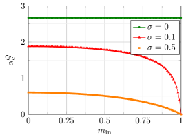
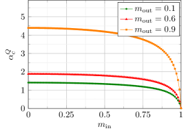
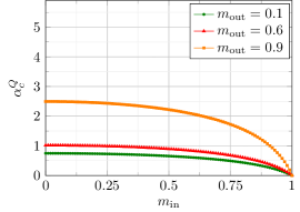
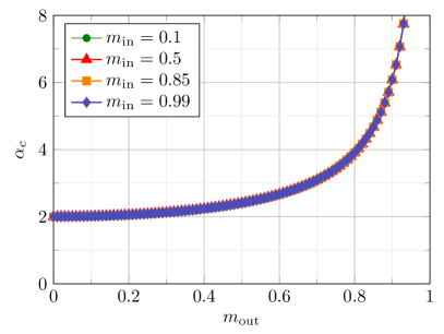
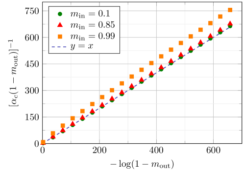
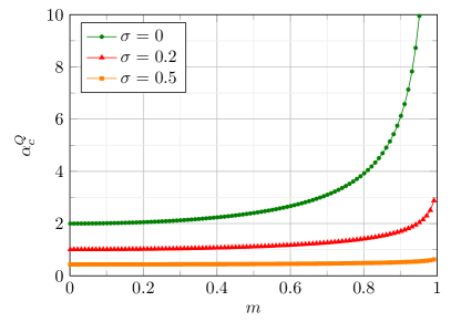
The numerical results obtained by solving equations (24) and (28) for several values of $m_{\mathrm{in}}$, $m_{\mathrm{out}}$ and $\tilde{\kappa}$ are shown in Figure 1 and Figure 2. Since the storage capacity depends solely on $\widetilde{\kappa}=\kappa+\sigma\Phi^{-1}(1-\epsilon)$, we kept fixed the values $\epsilon=0.01,\kappa=0$ and considered different values of $\sigma$, which also allows us to recover the classical limit for $\sigma=0$. A striking feature which distinguishes the quantum perceptron from the classical one is the dependence of the storage capacity on the bias $m_{\mathrm{in}}$, which is not present in the classical case with zero stability $\kappa=0$ (see the left panel of Figure 1). More precisely, as soon as $\sigma>0$, increasing the value of $|m_{\mathrm{in}}|$ while keeping fixed the value of $m_{\mathrm{out}}$ always decreases the storage capacity $\alpha_{c}^{Q}$. On the other hand, a common feature with the classical case is the divergence of the storage capacity when $m_{\mathrm{out}}\rightarrow 1$, for each fixed value of $m_{\mathrm{in}}$ (see Figure 2) The asymptotic behaviour in this limit (see Appendix B for the analytic derivation) is given by (see also Figure 3):

$$\alpha_{c}^{Q}\simeq-\frac{1}{(1-m_{\mathrm{out}})\log(1-m_{\mathrm{out}})}\ ,$$ (30)

confirming the result obtained for the classical scenario.

Figure 3: Limit $\alpha_{c}$ for $m_{\mathrm{out}}\rightarrow 1$, showing that the convergence to the asymptotic behaviour (30), represented here by the line $y=x+q$, holds for several values of $m_{\mathrm{in}}$, although the onset of the asymptotic behaviour appears later for $m_{\mathrm{in}}$ close to one.

Remark 4

An interesting feature emerging by differentiating the bias of the patterns $m_{\mathrm{in}}$ from the bias of target classification $m_{\mathrm{out}}$ is that even if the quantum storage capacity depends on $m_{\mathrm{in}}$ for each fixed $0\leqslant m_{\mathrm{out}}\leqslant 1$, the asymptotic behaviour when $m_{\mathrm{out}}\to 1^{-}$ does not depend on the pattern biases $m_{\mathrm{in}}$.

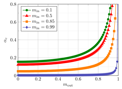
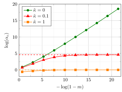
Even if the asymptotic behaviour (30) does not show a dependence on the patterns bias $m_{\mathrm{in}}$, one can see from Figure 2 and Figure 3 that as the input bias $m_{\mathrm{in}}$ increases, higher values of $m_{\mathrm{out}}$ are required to observe the asymptotic behaviour for the quantum perceptron. This is in contrast with the behaviour of the classical perceptron, where there is no dependence at all on $m_{\mathrm{in}}$ (see again Figure 2). In other words, values of $m_{\mathrm{in}}$ closer to $1$ slow down the attainment of the asymptotic behaviour in the quantum case, which motivates the investigation of the joint limit $m_{\mathrm{in}}=m_{\mathrm{out}}=m\rightarrow 1$. The results obtained (see Figure 4) show another striking difference between the classical and the quantum perceptron, that is, while classically the storage capacity diverges when $m\rightarrow 1$, in the quantum case this divergence is suppressed. In particular, from the analytic asymptotic expressions (see Appendix C) we obtain that the asymptotic behaviour in the quantum scenario reads

$$\alpha_{c}^{Q}\sim\frac{1}{\tilde{\kappa}^{2}},$$ (31)

which is finite for all values of $\sigma>0$, $0\leq\epsilon<1/2$, while we recover the classical divergence (for $\kappa=0$) in the classical limit $\sigma=0$.

Figure 4: (Left) $\alpha_{c}^{Q}$ plotted against $m=m_{\mathrm{in}}=m_{\mathrm{out}}$. Increasing the value of the bias $|m|$ always increases the storage capacity. (Right) Limit $\alpha_{c}^{Q}$ for $m_{\mathrm{out}}=m_{\mathrm{in}}=m\rightarrow 1$, for several values of $\tilde{\kappa}$. The case $\tilde{\kappa}=0$ corresponds to the classical case with $\kappa=0$, where the storage capacity diverges in the limit. In the quantum scenario ($\tilde{\kappa}>0$) the divergence is suppressed. The dashed lines correspond the asymptotic value $\alpha_{c}\sim 1/\tilde{\kappa}^{2}$

Remark 5

Figure 1 shows that for $\kappa=0$ the separation between curves corresponding to different values of $m_{\mathrm{out}}$ is reduced in the quantum regime. This is in contrast to what happens for curves corresponding to different values of $m_{\mathrm{in}}$, as shown in Fig.2.

5 Discussion and conclusion

Summarizing, we studied the storage capacity of the continuous variable model of quantum perceptron presented in Ref. [20] in the presence of a bias in the distribution of the patterns and their corresponding classifications. Besides the advantage of allowing an almost entirely analytical study, such a model admits the classical perceptron as a classical limit, thus allowing for a direct comparison of the storage performances in the two cases. We found that the additional randomness introduced in the quantum model gives rise to an effective increment in the stability parameter used in Gardner’s statistical approach, $\kappa\rightarrow\tilde{\kappa}$, which gives rise to several peculiar features that are not observed in the classical case with zero stability.

For instance, the possibility of indefinitely enhancing the storage capacity by increasing the bias of the patterns and their classifications is prevented at the quantum level. Moreover, in contrast to the classical case, when the bias of the patterns and the bias in their corresponding classifications are varied separately, a dependence of the storage capacity on the input patterns’ bias appears even when the stability parameter reduces to zero. Overall, however, the performance of the quantum perceptron model remains below that of the classical one. This is likely due to the fact that the considered quantum model introduces two sources of randomness: one due to the encoding of patterns by means of non-zero width Gaussian states and another one due to the final measurement operation implementing the classical non-linear activation function. It is worth stressing that the modification in the effective threshold $\tilde{\kappa}-\kappa=\sigma\Phi^{-1}(1-\epsilon)$ contains both the contribution of randomness coming from the width $\sigma$ of the Gaussian encoding of the patterns, and the statistical error due to the quantum measurement $\epsilon$: as a consequence, the worsening of the quantum storage capacity with respect to the classical one cannot be ascribed to only one of them. These results clearly point to the necessity of considering multi-layer quantum perceptrons to hope for quantum advantages of the sort coming from linear superpositions and entanglement.

Appendix A Derivation of the main result

In order to extract the large $N$ behavior of $\braket{{[V^{Q}_{N}(\boldsymbol{x}^{\mu},\xi^{\mu},\kappa,\sigma,\epsilon)]}^{n}}$ in Eq.(32), we recast it as

$$\langle{[V^{Q}_{N}(\boldsymbol{x}^{\mu},\xi^{\mu},\kappa,\sigma,\epsilon)]}^{n}\rangle=\frac{1}{Z^{n}_{N}}\int_{\mathbb{R}^{nN}}\mathop{}\mathrm{d}^{nN}\boldsymbol{W}~{}\delta_{N}^{(n)}(\|\boldsymbol{W}\|^{2})\,{A(\boldsymbol{W})}\ ,$$ (32)

with

$$A(\boldsymbol{W}):=\left\langle\prod_{\mu=1}^{p}\prod_{\gamma=1}^{n}\Theta({R_{\kappa,\sigma}(\boldsymbol{w}_{\gamma},\boldsymbol{x}^{\mu},\xi^{\mu})}-1+\epsilon)\right\rangle_{\boldsymbol{x},\xi}\ .$$ (33)

Using the distributional expression

$$\Theta(x-u)=\int_{u}^{+\infty}\mathop{}\mathrm{d}\lambda\ \delta(\lambda-x)=\int_{u}^{+\infty}\mathop{}\mathrm{d}\lambda\ {\int_{-\infty}^{+\infty}}\frac{\mathop{}\mathrm{d}y}{2\pi}\ \mathop{}\mathrm{e}^{\mathop{}\mathrm{i}y(\lambda-x)},$$ (34)

we express the Heaviside function in (33) as

$$\Theta({R_{\kappa,\sigma}(\boldsymbol{w}_{\gamma},\boldsymbol{x}^{\mu},\xi^{\mu})}-1+\epsilon)=\int_{1-\epsilon}^{+\infty}\mathop{}\mathrm{d}\lambda_{\gamma}^{\mu}\ {\int_{-\infty}^{+\infty}}\frac{\mathop{}\mathrm{d}y_{\gamma}^{\mu}}{2\pi}\ \mathop{}\mathrm{e}^{\mathop{}\mathrm{i}y_{\gamma}^{\mu}(\lambda_{\gamma}^{\mu}-{R_{\kappa,\sigma}(\boldsymbol{w}_{\gamma},\boldsymbol{x}^{\mu},\xi^{\mu})})},$$ (35)

so that

$$A(\boldsymbol{W})=\frac{1}{(2\pi)^{nP}}\int_{[1-\epsilon,+\infty)^{nP}}\hskip-28.45274pt\mathop{}\mathrm{d}^{nP}\boldsymbol{\Lambda}{\int_{\mathbb{R}^{nP}}}\mathop{}\mathrm{d}^{nP}\boldsymbol{Y}\ \mathop{}\mathrm{e}^{\mathop{}\mathrm{i}\sum_{\mu=1}^{p}\sum_{\gamma=1}^{n}y_{\gamma}^{\mu}\lambda_{\gamma}^{\mu}}\,B(\boldsymbol{Y},\boldsymbol{W})\ ,$$ (36)

where we introduced the symbols

$$\mathop{}\mathrm{d}^{nP}\boldsymbol{\Lambda}\equiv\prod_{\mu=1}^{p}\prod_{\gamma=1}^{n}\mathop{}\mathrm{d}\lambda_{\gamma}^{\mu}\ ,\ \mathop{}\mathrm{d}^{nP}\boldsymbol{Y}\equiv\prod_{\mu=1}^{p}\prod_{\gamma=1}^{n}\mathop{}\mathrm{d}y_{\gamma}^{\mu}\ ,$$ (37)

and the quantity

$$B(\boldsymbol{Y},\boldsymbol{W})\equiv\left\langle\prod_{\gamma=1}^{n}\prod_{\mu=1}^{p}~{}\mathop{}\mathrm{e}^{-\mathop{}\mathrm{i}y_{\gamma}^{\mu}{R_{\kappa,\sigma}(\boldsymbol{w}_{\gamma},\boldsymbol{x}^{\mu},\xi^{\mu})}}\right\rangle_{\boldsymbol{x},\xi}\ .$$ (38)

To proceed, it is convenient to use (see (27))

$$\Phi(x)\equiv\frac{1}{\sqrt{2\pi}}\int_{-\infty}^{x}\mathop{}\mathrm{d}u\ e^{-u^{2}/2}$$

and rewrite (10) as

$${R_{\kappa,\sigma}(\boldsymbol{w}_{\gamma},\boldsymbol{x}^{\mu},\xi^{\mu})}=\int_{-\infty}^{+\infty}\mathop{}\mathrm{d}s\ P_{\boldsymbol{w}_{\gamma},\boldsymbol{{x}}^{\mu},\sigma}(s)\ \Theta\left(\xi^{\mu}\frac{s}{||\boldsymbol{w}||}-\kappa\right)=\Phi\left(-\frac{\kappa}{\sigma}+\xi^{\mu}\frac{\boldsymbol{x}^{\mu}\cdot\boldsymbol{w}_{\gamma}}{||\boldsymbol{w}_{\gamma}||\sigma}\right).$$ (39)

Then, using the exponential representation of the Dirac delta and the statistical independence of patterns and targets with different indices, one gets

$$B(\boldsymbol{Y},\boldsymbol{W}) =\left\langle\prod_{\mu=1}^{p}\prod_{\gamma=1}^{n}\mathop{}\mathrm{e}^{-\mathop{}\mathrm{i}y_{\gamma}^{\mu}\Phi\left(-\frac{\kappa}{\sigma}+\xi^{\mu}\frac{\boldsymbol{x}^{\mu}\cdot\boldsymbol{w}_{\gamma}}{||\boldsymbol{w}_{\gamma}||\sigma}\right)}\right\rangle_{\boldsymbol{x}^{\mu},\xi^{\mu}}$$

$$=\left\langle\prod_{\mu=1}^{p}\prod_{\gamma=1}^{n}\int_{\mathbb{R}}\mathop{}\mathrm{d}\eta^{\mu}_{\gamma}\ \delta\left(\eta^{\mu}_{\gamma}+\frac{\kappa}{\sigma}-\xi^{\mu}\frac{\boldsymbol{x}^{\mu}\cdot\boldsymbol{w}_{\gamma}}{||\boldsymbol{w}_{\gamma}||\sigma}\right)\,\mathop{}\mathrm{e}^{-\mathop{}\mathrm{i}y_{\gamma}^{\mu}\Phi\left(\eta^{\mu}_{\gamma}\right)}\right\rangle_{\boldsymbol{x},\xi}$$

$$={\frac{1}{(2\pi)^{nP}}\int_{\mathbb{R}^{2nP}}\mathop{}\mathrm{d}^{nP}\boldsymbol{\Omega}\mathop{}\mathrm{d}^{nP}\boldsymbol{H}~{}C(\boldsymbol{\Omega},\boldsymbol{W})}$$

$${\qquad\qquad\qquad\qquad\times\exp\Bigg{[}-i\sum_{\mu=1}^{p}\sum_{\gamma=1}^{n}\left(\eta^{\mu}_{\gamma}+\frac{\kappa}{\sigma}\right)\omega_{\gamma}^{\mu}-i\sum_{\mu=1}^{p}\sum_{\gamma=1}^{n}y^{\mu}_{\gamma}\Phi(\eta^{\mu}_{\gamma})\Bigg{]}}\ ,$$ (40)

with

$$C(\boldsymbol{\Omega},\boldsymbol{W}):=\prod_{\mu=1}^{p}\left\langle\exp\left(\mathop{}\mathrm{i}\xi^{\mu}\sum_{\gamma=1}^{n}\omega^{\mu}_{\gamma}\frac{\boldsymbol{x}^{\mu}\cdot\boldsymbol{w}_{\gamma}}{\sigma\sqrt{N}}\right)\right\rangle_{\boldsymbol{x},\xi}\ ,$$ (41)

where $\boldsymbol{\Omega}=\{\omega^{\mu}_{\gamma}\}_{\mu,\gamma}$, $\boldsymbol{H}=\{\eta^{\mu}_{\gamma}\}_{\mu,\gamma}$ and

$$\mathop{}\mathrm{d}^{nP}\boldsymbol{\Omega}\mathop{}\mathrm{d}^{nP}\boldsymbol{H}=\prod_{\mu=1}^{P}\prod_{\gamma=1}^{n}\mathop{}\mathrm{d}\omega_{\gamma}^{\mu}\mathop{}\mathrm{d}\eta^{\mu}_{\gamma}\ .$$ (42)

Since the patterns have components $x^{\mu}_{j}=\pm 1$ which are statistically independent and identically distributed, using (17), one computes the mean over the patterns in $C(\boldsymbol{\Omega},\boldsymbol{W})$ as follows:

$${C(\boldsymbol{\Omega},\boldsymbol{W})} =\prod_{\mu=1}^{p}\prod_{j=1}^{N}\Big{\langle}\exp\Bigg{(}\mathop{}\mathrm{i}\xi^{\mu}\sum_{\gamma=1}^{n}\omega^{\mu}_{\gamma}\frac{w_{\gamma,j}x^{\mu}_{j}}{\sigma\sqrt{N}}\Bigg{)}\Big{\rangle}_{x_{j}^{\mu},\xi^{\mu}}$$

$$=\prod_{\mu=1}^{p}\prod_{j=1}^{N}\frac{1}{2}\Bigg{\langle}\exp\Bigg{(}\mathop{}\mathrm{i}\xi^{\mu}\sum_{\gamma=1}^{n}\frac{w_{\gamma,j}\omega^{\mu}_{\gamma}}{\sigma\sqrt{N}}\Bigg{)}+\exp\Bigg{(}-\mathop{}\mathrm{i}\xi^{\mu}\sum_{\gamma=1}^{n}\frac{w_{\gamma,j}\omega^{\mu}_{\gamma}}{\sigma\sqrt{N}}\Bigg{)}$$

$$\qquad+m_{\mathrm{in}}\Bigg{(}\exp\Bigg{(}\mathop{}\mathrm{i}\xi^{\mu}\sum_{\gamma=1}^{n}\frac{w_{\gamma,j}\omega^{\mu}_{\gamma}}{\sigma\sqrt{N}}\Bigg{)}-\exp\Bigg{(}-\mathop{}\mathrm{i}\xi^{\mu}\sum_{\gamma=1}^{n}\frac{w_{\gamma,j}\omega^{\mu}_{\gamma}}{\sigma\sqrt{N}}\Bigg{)}\Bigg{)}\Bigg{\rangle}_{\xi^{\mu}}$$

$$=\prod_{\mu=1}^{p}\prod_{j=1}^{N}\left\langle\cos{\Bigg{(}\xi^{\mu}\sum_{\gamma=1}^{n}\frac{w_{\gamma,j}\omega^{\mu}_{\gamma}}{\sigma\sqrt{N}}\Bigg{)}}+\mathop{}\mathrm{i}m_{\mathrm{in}}\sin{\Bigg{(}\xi^{\mu}\sum_{\gamma=1}^{n}\frac{w_{\gamma,j}\omega^{\mu}_{\gamma}}{\sigma\sqrt{N}}\Bigg{)}}\right\rangle_{\xi^{\mu}}$$

$$=\prod_{\mu=1}^{p}\prod_{j=1}^{N}\left\langle\exp{\Bigg{(}\log\left[\cos{\Bigg{(}\xi^{\mu}\sum_{\gamma=1}^{n}\frac{w_{\gamma,j}\omega^{\mu}_{\gamma}}{\sigma\sqrt{N}}\Bigg{)}}+\mathop{}\mathrm{i}m_{\mathrm{in}}\sin{\Bigg{(}\xi^{\mu}\sum_{\gamma=1}^{n}\frac{w_{\gamma,j}\omega^{\mu}_{\gamma}}{\sigma\sqrt{N}}\Bigg{)}}\right]\Bigg{)}}\right\rangle_{\xi^{\mu}}.$$

When $N\gg 1$, the leading order expansion in $1/N$ of each factor in the product over the $\mu$ index reads

$$\prod_{j=1}^{N}\left\langle\exp\Bigg{(}\log\Bigg{[}1+\mathop{}\mathrm{i}m_{\mathrm{in}}\Bigg{(}\xi^{\mu}\sum_{\gamma=1}^{n}\frac{w_{\gamma,j}\omega^{\mu}_{\gamma}}{\sigma\sqrt{N}}\Bigg{)}-\frac{1}{2}\Bigg{(}\xi^{\mu}\sum_{\gamma=1}^{n}\frac{w_{\gamma,j}\omega^{\mu}_{\gamma}}{\sigma\sqrt{N}}\Bigg{)}^{2}\Bigg{]}\Bigg{)}\right\rangle_{\xi^{\mu}}$$

$$=\prod_{j=1}^{N}\left\langle\exp\Bigg{(}\log\Bigg{(}1+\mathop{}\mathrm{i}m_{\mathrm{in}}\Bigg{(}\xi^{\mu}\sum_{\gamma=1}^{n}\frac{w_{\gamma,j}\omega^{\mu}_{\gamma}}{\sigma\sqrt{N}}\Bigg{)}-\frac{1}{2\sigma^{2}N}\sum_{\beta=1}^{n}w_{\beta,j}\,\omega^{\mu}_{\beta}\sum_{\gamma=1}^{n}w_{\gamma,j}\,\omega^{\mu}_{\gamma}\Bigg{)}\Bigg{)}\right\rangle_{\xi^{\mu}}$$

$$=\prod_{j=1}^{N}\left\langle\exp\Bigg{(}\mathop{}\mathrm{i}m_{\mathrm{in}}\Bigg{(}\xi^{\mu}\sum_{\gamma=1}^{n}\frac{w_{\gamma,j}\omega^{\mu}_{\gamma}}{\sigma\sqrt{N}}\Bigg{)}-\frac{1-m_{\mathrm{in}}^{2}}{2\sigma^{2}N}\sum_{\beta=1}^{n}w_{\beta,j}\omega^{\mu}_{\beta}\sum_{\gamma=1}^{n}{w}_{\gamma,j}\omega^{\mu}_{\gamma}\Bigg{)}\right\rangle_{\xi^{\mu}}$$

$$=\left\langle\exp{\Bigg{(}\mathop{}\mathrm{i}m_{\mathrm{in}}\xi^{\mu}\sum_{\gamma=1}^{n}\sum_{j=1}^{N}\frac{w_{\gamma,j}\omega^{\mu}_{\gamma}}{\sigma\sqrt{N}}-\frac{1-m_{\mathrm{in}}^{2}}{2\sigma^{2}N}\sum_{\gamma,\beta=1}^{n}\omega^{\mu}_{\gamma}\omega^{\mu}_{\beta}\sum_{j=1}^{N}{w}_{\gamma,j}w_{\beta,j}\Bigg{)}}\right\rangle_{\xi^{\mu}}\ ,$$ (43)

the remaining terms vanishing as $O\left(1/\sqrt{N}\right)$. Using $\|\boldsymbol{w}_{\gamma}\|^{2}=N$ and setting

$$M_{\gamma}\equiv\frac{1}{\sqrt{N}}\sum_{j=1}^{N}w_{\gamma,j}\ ,\quad q_{\gamma\beta}\equiv\frac{1}{N}\sum_{j=1}^{N}{w}_{\gamma,j}{w}_{\beta,j}$$ (44)

for $\gamma,\beta=1,\dots,n$, $\gamma>\beta$, we finally focus upon

$${C(\boldsymbol{\Omega},\boldsymbol{W})}{\simeq}\prod_{\mu=1}^{p}\left\langle\exp\Bigg{(}\frac{\mathop{}\mathrm{i}m_{\mathrm{in}}\xi^{\mu}}{\sigma}\sum_{\gamma=1}^{n}M_{\gamma}\omega^{\mu}_{\gamma}-\frac{1-m_{\mathrm{in}}^{2}}{2\sigma^{2}}\Bigg{[}\sum_{\gamma=1}^{n}(\omega_{\gamma}^{\mu})^{2}+2\sum_{{\gamma>\beta=1}}^{n}\omega_{\beta}^{\mu}\omega_{\gamma}^{\mu}q_{\gamma\beta}\Bigg{]}\Bigg{)}\right\rangle_{\xi^{\mu}}\ ,$$ (45)

neglecting corrections of order $O\left(1/\sqrt{N}\right)$. Therefore, to leading order in $1/N$, Eq. (40) becomes

$$B(\boldsymbol{Y},\boldsymbol{W}){\simeq}\frac{1}{(2\pi)^{nP}}\int_{\mathbb{R}^{2np}}\mathop{}\mathrm{d}^{nP}\boldsymbol{\Omega}\mathop{}\mathrm{d}^{nP}\boldsymbol{H}\,\exp\Bigg{[}-i\sum_{\mu=1}^{p}\sum_{\gamma=1}^{n}\left(\eta^{\mu}_{\gamma}+\frac{\kappa}{\sigma}\right)\omega_{\gamma}^{\mu}-i\sum_{\mu=1}^{p}\sum_{\gamma=1}^{n}y^{\mu}_{\gamma}\Phi(\eta^{\mu}_{\gamma})\Bigg{]}$$

$$\hskip 28.45274pt\times\prod_{\mu=1}^{p}\left\langle\exp\Bigg{(}\frac{\mathop{}\mathrm{i}m_{\mathrm{in}}\xi^{\mu}}{\sigma}\sum_{\gamma=1}^{n}M_{\gamma}\omega^{\mu}_{\gamma}-\frac{1-m_{\mathrm{in}}^{2}}{2\sigma^{2}}\Bigg{[}\sum_{\gamma=1}^{n}(\omega_{\gamma}^{\mu})^{2}+2\sum_{{\gamma>\beta=1}}^{n}\omega_{\beta}^{\mu}\omega_{\gamma}^{\mu}q_{\gamma\beta}\Bigg{]}\Bigg{)}\right\rangle_{\xi^{\mu}}\ \Bigg{)}.$$ (46)

Since the integrals for different $\mu$’s are the same and the targets $\xi^{\mu}$ are statistically independent and equally distributed, Eq.(36) reduces to

$$A(\boldsymbol{W})=\left(\frac{1}{(2\pi)^{2n}}\int_{[1-\epsilon,+\infty)^{n}}\hskip-28.45274pt\mathop{}\mathrm{d}^{n}\boldsymbol{\lambda}\ \int_{\mathbb{R}^{3n}}\hskip-14.22636pt\mathop{}\mathrm{d}^{n}\boldsymbol{y}\mathop{}\mathrm{d}^{n}\boldsymbol{\eta}\mathop{}\mathrm{d}^{n}\boldsymbol{\omega}\,\left\langle\mathop{}\mathrm{e}^{{K_{\xi}\left(\boldsymbol{\eta},\boldsymbol{\lambda},\boldsymbol{y},\boldsymbol{\omega},\boldsymbol{Q},\boldsymbol{M}\right)}}\right\rangle_{\xi}\right)^{p},$$ (47)

where $\boldsymbol{\eta}=\{\eta_{\gamma}\}$, $\boldsymbol{y}=\{y_{\gamma}\}$, $\boldsymbol{\lambda}=\{\lambda_{\gamma}\}$, $\boldsymbol{\omega}=\{\omega_{\gamma}\}$, $\boldsymbol{Q}=\{q_{\alpha\beta}\}$, $\boldsymbol{M}=\{M_{\gamma}\}$, for $\alpha,\beta,\gamma=1,\ldots,n$,

$$\mathop{}\mathrm{d}^{n}\boldsymbol{\lambda}\equiv\prod_{\gamma=1}^{n}\mathop{}\mathrm{d}\lambda_{\gamma}\ ,\ \mathop{}\mathrm{d}^{n}\boldsymbol{y}\equiv\prod_{\gamma=1}^{n}\mathop{}\mathrm{d}y_{\gamma}\ ,\ \mathop{}\mathrm{d}^{n}\boldsymbol{\eta}\equiv\prod_{\gamma=1}^{n}\mathop{}\mathrm{d}\eta_{\gamma}\ ,\ \mathop{}\mathrm{d}^{n}\boldsymbol{\omega}\equiv\prod_{\gamma=1}^{n}\mathop{}\mathrm{d}\omega_{\gamma}$$

and

$$K_{\xi}\left(\boldsymbol{\eta},\boldsymbol{\lambda},\boldsymbol{y},\boldsymbol{\omega},\boldsymbol{Q},\boldsymbol{M}\right)\equiv\mathop{}\mathrm{i}\sum_{\gamma=1}^{n}\left[y_{\gamma}\lambda_{\gamma}-y_{\gamma}\Phi(\eta_{\gamma})-\left(\frac{\kappa-\xi m_{\mathrm{in}}M_{\gamma}}{\sigma}+\eta_{\gamma}\right)\omega_{\gamma}\right]$$ (48)

$$\hskip 56.9055pt-\frac{1-m_{\mathrm{in}}^{2}}{2\sigma^{2}}\Bigg{(}\sum_{\gamma=1}^{n}(\omega_{\gamma})^{2}+2\sum_{\gamma\neq\beta=1}^{n}\omega_{\beta}\omega_{\gamma}q_{\gamma\beta}\Bigg{)}.$$

Writing the various Dirac deltas appearing in (32) as

$$\delta\Big{(}||\boldsymbol{w}_{\gamma}||^{2}-N\Big{)}=\int_{-\infty}^{+\infty}\frac{\mathop{}\mathrm{d}E_{\gamma}}{4\pi}\ \mathop{}\mathrm{e}^{-\mathop{}\mathrm{i}\frac{E_{\gamma}}{2}N+\mathop{}\mathrm{i}\frac{E_{\gamma}}{2}\sum_{j=1}^{N}{w}_{\gamma,j}^{2}},$$ (50)

as well as those Dirac deltas whose integration over $q_{\gamma\beta}$, respectively $M_{\gamma}$, implements the constraints (44) within (47), as

$$\delta\Bigg{(}q_{\gamma\beta}-\frac{1}{N}\sum_{j=1}^{N}{w}_{\gamma,j}{w}_{\beta,j}\Bigg{)} =N\int_{-\infty}^{+\infty}\ \frac{\mathop{}\mathrm{d}F_{\gamma\beta}}{2\pi}\ \exp\Bigg{(}-\mathop{}\mathrm{i}Nq_{\gamma\beta}F_{\alpha\beta}+\mathop{}\mathrm{i}F_{\gamma\beta}\sum_{j=1}^{N}{w_{\gamma,j}w_{\beta,j}}\Bigg{)}\ ,$$ (51)

$$\delta\Bigg{(}M_{\gamma}-\frac{1}{\sqrt{N}}\sum_{j=1}^{N}{w_{\gamma,j}}\Bigg{)} =\sqrt{N}\int_{-\infty}^{+\infty}\frac{\mathop{}\mathrm{d}{L_{\gamma}}}{2\pi}\ \exp\Bigg{(}-\mathop{}\mathrm{i}\sqrt{N}L_{\gamma}M_{\gamma}+\mathop{}\mathrm{i}\,L_{\gamma}\sum_{j=1}^{N}w_{\gamma,j}\Bigg{)},$$ (52)

and inserting them into (32), one finally arrives at the following explicit integral expression

$$\hskip-25.6073pt~{}\langle{[V^{Q}_{N}(\boldsymbol{x}^{\mu},\xi^{\mu},\kappa,\sigma,\epsilon)]}^{n}\rangle={\frac{(N)^{n^{2}/2}}{Z_{N}^{n}}\int_{\mathbb{R}^{nN+n^{2}+2n}}\prod_{\gamma=1}^{n}\prod_{j=1}^{N}\prod_{\gamma<\beta=1}^{n}\mathop{}\mathrm{d}w_{\gamma,j}\frac{\mathop{}\mathrm{d}E_{\gamma}}{4\pi}\mathop{}\mathrm{d}M_{\gamma}\mathop{}\mathrm{d}q_{\gamma\beta}\,\frac{\mathop{}\mathrm{d}F_{\gamma\beta}}{2\pi}\,\frac{\mathop{}\mathrm{d}{L_{\gamma}}}{2\pi}}$$

$$\hskip 28.45274pt\times\exp\Bigg{(}-i\frac{E_{\gamma}}{2}N+\mathop{}\mathrm{i}\frac{E_{\gamma}}{2}\sum_{j=1}^{N}w_{\gamma,j}^{2}\Bigg{)}\,\exp\Bigg{(}-\mathop{}\mathrm{i}Nq_{\gamma\beta}F_{\gamma\beta}+\mathop{}\mathrm{i}F_{\gamma\beta}\sum_{j=1}^{N}w_{\gamma,j}\,w_{\beta,j}\Bigg{)}$$

$$\hskip 56.9055pt\times{\exp\Bigg{(}-\mathop{}\mathrm{i}\sqrt{N}M_{\gamma}{L_{\gamma}}+\mathop{}\mathrm{i}L_{\gamma}\sum_{j=1}^{N}w_{\gamma,j}\Bigg{)}}$$

$$\hskip 85.35826pt\times~{}{\Bigg{[}\int_{1-\epsilon}^{+\infty}\frac{1}{(2\pi)^{2n}}\int_{[1-\epsilon,+\infty)^{n}}\hskip-28.45274pt\mathop{}\mathrm{d}^{n}\boldsymbol{\lambda}\ \int_{\mathbb{R}^{3n}}\hskip-14.22636pt\mathop{}\mathrm{d}^{n}\boldsymbol{y}\mathop{}\mathrm{d}^{n}\boldsymbol{\eta}\mathop{}\mathrm{d}^{n}\boldsymbol{\omega}\,\left\langle\mathop{}\mathrm{e}^{{K_{\xi}\left(\boldsymbol{\eta},\boldsymbol{\lambda},\boldsymbol{y},\boldsymbol{\omega},\boldsymbol{Q},\boldsymbol{M}\right)}}\right\rangle_{\xi}\Bigg{]}^{p}}\ .$$

Regrouping together the integrals over $w_{\gamma,j}$ with different $j$ and same $\gamma$, one writes

$$~{}\langle{[V^{Q}_{N}(\boldsymbol{x}^{\mu},\xi^{\mu},\kappa,\sigma,\epsilon)]}^{n}\rangle ={\frac{N^{n^{2}/2}}{Z_{N}^{n}}\int_{\mathbb{R}^{n^{2}+2n}}\prod_{\gamma=1}^{n}\prod_{\gamma<\beta=1}^{n}\frac{\mathop{}\mathrm{d}E_{\gamma}}{4\pi}\mathop{}\mathrm{d}M_{\gamma}\mathop{}\mathrm{d}q_{\gamma\beta}\,\frac{\mathop{}\mathrm{d}F_{\gamma\beta}}{2\pi}\,\frac{\mathop{}\mathrm{d}{L_{\gamma}}}{2\pi}}$$

$$\hskip 56.9055pt\times\Bigg{[}\exp\Bigg{(}{-}\frac{\mathop{}\mathrm{i}}{2}\sum_{\gamma=1}^{n}E_{\gamma}-\mathop{}\mathrm{i}\sum_{\gamma<\beta=1}^{n}F_{\gamma\beta}q_{\gamma,\beta}-\frac{\mathop{}\mathrm{i}}{\sqrt{N}}\sum_{\gamma=1}^{n}L_{\gamma}\,M_{\gamma}\Bigg{)}\Bigg{]}^{N}$$

$$\times\Bigg{[}\int_{\mathbb{R}^{n}}\prod_{\gamma=1}^{n}\mathop{}\mathrm{d}w_{\gamma}\exp\Bigg{(}\mathop{}\mathrm{i}\sum_{\gamma<\beta=1}^{n}F_{\gamma\beta}{w}_{\gamma}{w}_{\beta}{+}\frac{\mathop{}\mathrm{i}}{2}\sum_{\gamma=1}^{n}\,E_{\gamma}\,w_{\gamma}^{2}+\mathop{}\mathrm{i}\sum_{\gamma=1}^{n}{L_{\gamma}}\,w_{\gamma}\Bigg{)}\Bigg{]}^{N}$$

$$\hskip 28.45274pt\times~{}{\Bigg{[}\frac{1}{(2\pi)^{2n}}\int_{[1-\epsilon,+\infty)^{n}}\hskip-28.45274pt\mathop{}\mathrm{d}^{n}\boldsymbol{\lambda}\ \int_{\mathbb{R}^{3n}}\hskip-14.22636pt\mathop{}\mathrm{d}^{n}\boldsymbol{y}\mathop{}\mathrm{d}^{n}\boldsymbol{\eta}\mathop{}\mathrm{d}^{n}\boldsymbol{\omega}\,\left\langle\mathop{}\mathrm{e}^{{K_{\xi}\left(\boldsymbol{\boldsymbol{\eta},\lambda},\boldsymbol{y},\boldsymbol{\omega},\boldsymbol{Q},\boldsymbol{M}\right)}}\right\rangle_{\xi}\Bigg{]}^{p}}\ .$$

In the large $N$ limit, the contribution $\frac{1}{\sqrt{N}}\sum_{\gamma=1}^{n}{L_{\gamma}}M_{\gamma}$ can be neglected; using (13), at leading order in $N\gg 1$, one gets

$$\langle{[V^{Q}_{N}(\boldsymbol{x}^{\mu},\xi^{\mu},\kappa,\sigma,\epsilon)]}^{n}\rangle ={\frac{N^{n^{2}/2}}{Z_{N}^{n}}\int_{\mathbb{R}^{3n}}}\left(\prod_{\gamma=1}^{n}\frac{\mathop{}\mathrm{d}E_{\gamma}}{4\pi}\mathop{}\mathrm{d}M_{\gamma}\frac{\mathop{}\mathrm{d}L_{\gamma}}{2\pi}\right)\int_{{\mathbb{R}^{n^{2}-n}}}~{}\left(\prod_{\gamma>\beta=1}^{n}\mathop{}\mathrm{d}q_{\gamma\beta}\frac{\mathop{}\mathrm{d}F_{\gamma\beta}}{2\pi}\right)$$

$$\times\exp\Big{(}N\,G(\mathbf{E},\mathbf{F},\mathbf{L},\mathbf{M},\mathbf{Q})\Big{)}\ ,$$ (53)

where $\mathbf{E}=\{E_{\gamma}\}_{\gamma=1}^{n}$, $\mathbf{F}=\{F_{\gamma\beta}\}_{\gamma>\beta=1}^{n}$, $\mathbf{L}=\{L_{\gamma}\}_{\gamma=1}^{n}$, and

$$\ G(\mathbf{E},\mathbf{F},\mathbf{L},\mathbf{M},\mathbf{Q})\equiv\frac{p}{N}\,G_{1}(\mathbf{M},\mathbf{Q})+G_{2}(\mathbf{E},\mathbf{F},\mathbf{L})+G_{3}(\mathbf{E},\mathbf{F},\mathbf{Q})\ ,$$ (54)

with

$$~{}{G_{1}(\mathbf{M},\mathbf{Q})}=\log\left[\int_{{[1-\epsilon,+\infty)^{n}}}\left(\prod_{\gamma=1}^{n}\frac{\mathop{}\mathrm{d}\lambda_{\gamma}}{2\pi}\right)\int_{~{}}^{~{}}\left(\prod_{\gamma=1}^{n}\frac{\mathop{}\mathrm{d}y_{\gamma}\mathop{}\mathrm{d}\eta_{\gamma}\mathop{}\mathrm{d}\omega_{\gamma}}{2\pi}\right)\left\langle\mathop{}\mathrm{e}^{{K_{\xi}\left(\boldsymbol{\eta},\boldsymbol{\lambda},\boldsymbol{y},\boldsymbol{\omega},\boldsymbol{Q},\boldsymbol{M}\right)}}\right\rangle_{\xi}\right],$$ (55)

$${G_{2}(\mathbf{E},\mathbf{F},\mathbf{L})}=\log\left[\int_{\mathbb{R}^{n}}\prod_{\gamma=1}^{n}\mathop{}\mathrm{d}w_{\gamma}\mathop{}\mathrm{e}^{\mathop{}\mathrm{i}\sum_{\gamma<\beta}^{~{}}F_{\gamma\beta}{w}_{\gamma}{w}_{\beta}{+}\mathop{}\mathrm{i}\sum_{\gamma=1}^{n}\frac{E_{\gamma}}{2}\,w_{\gamma}^{2}\,+\mathop{}\mathrm{i}\,\sum_{\gamma=1}^{n}w_{\gamma}L_{\gamma}}\right],$$ (56)

$${G_{3}(\mathbf{E},\mathbf{F},\mathbf{Q})}={-}\frac{\mathop{}\mathrm{i}}{2}\sum_{\gamma=1}^{n}E_{\gamma}-\mathop{}\mathrm{i}\,\sum_{\gamma>\beta}^{~{}}F_{\gamma\beta}q_{\gamma,\beta}\ .$$ (57)

A.1 Saddle-point approximation

When $N$ is large, the behaviour of $\langle[V^{Q}_{N}(\boldsymbol{x}^{\mu},\xi^{\mu},\kappa,\sigma,\epsilon)]^{n}\rangle$ can be obtained using the saddle-point approximation, as follows. Setting $\mathbf{z}\equiv(\mathbf{E},\mathbf{F},\mathbf{L},\mathbf{M},\mathbf{Q})$ and considering it as a vector in $\mathbb{C}^{n^{2}+2n}$, one expands $G(\mathbf{z})\equiv G(\mathbf{E},\mathbf{F},\mathbf{L},\mathbf{M},\mathbf{Q})$ around the stationary point $\mathbf{z}^{0}=(\mathbf{E}^{0},\mathbf{F}^{0},\mathbf{L}^{0},\mathbf{M}^{0},\mathbf{Q}^{0})$ such that $\displaystyle\frac{\partial G(\mathbf{z}^{0})}{\partial z_{k}}=0$:

$$G(\mathbf{z})\simeq G(\mathbf{z}^{0})+\frac{1}{2}\sum_{j,k=1}^{n^{2}+2n}\frac{\partial^{2}G(\mathbf{z}^{0})}{\partial z_{j}\partial z_{k}}\,(z_{j}-z^{0}_{j})\,(z_{k}-z^{0}_{k})\ .$$

Let $G^{\prime\prime}(\mathbf{z}^{0})\equiv\left[\frac{\partial^{2}G(\mathbf{z}^{0})}{\partial z_{j}\partial z_{k}}\right]$ be the Hessian $(n^{2}+2n)\times(n^{2}+2n)$ matrix at the stationary point. If such a matrix is negative semi-definite, by suitably deforming the integration paths into the complex domain, one can perform $n^{2}+2n$ Gaussian integrations by rescaling with $\sqrt{N}$ the corresponding integration variables and approximate:

$$\langle[V^{Q}_{N}(\boldsymbol{x}^{\mu},\xi^{\mu},\kappa,\sigma,\epsilon)]^{n}\rangle{\simeq}\frac{1}{Z_{N}^{n}}\,\frac{1}{N^{n}}\,\left(\sqrt{\frac{2\pi}{|\det G^{\prime\prime}(\mathbf{z}^{0})|}}\right)^{n^{2}+2n}\ \mathrm{e}^{NG(\mathbf{z}^{0})}\ .$$ (58)

From Eqs. (20) and (18), one needs to control the behaviour of the ratio $\displaystyle\frac{1}{nN}\log\langle[(V^{Q}_{N}(\boldsymbol{x}^{\mu},\xi^{\mu},\kappa,\sigma,\epsilon)]^{n}\rangle$ for $n\to 0^{+}$ and $N\to+\infty$. From Eq. (58) and using Eq. (14) one gets:

$$\frac{1}{nN}\log\langle[V^{Q}_{N}(\boldsymbol{x}^{\mu},\xi^{\mu},\kappa,\sigma,\epsilon)]^{n}\rangle=\frac{1}{n}\,G(\mathbf{z}^{0})-\frac{1}{2}\log(2\pi\mathrm{e})+O\left(\frac{\log N}{N}\right)\ .$$ (59)

A.2 Replica symmetric ansatz

Making use of the replica-symmetric ansatz which states that the stationary point $\mathbf{z}_{0}$ is replica-insensitive, one seeks it setting

$$q_{\gamma\beta}=q,\quad F_{\gamma\beta}=F,\quad E_{\gamma}=E\quad M_{\gamma}=M\quad\text{and}\quad L_{\gamma}=L,$$ (60)

so that (48) becomes

$${K_{\xi}\left(\boldsymbol{\eta},\boldsymbol{\lambda},\boldsymbol{y},\boldsymbol{\omega},q,\boldsymbol{M}\right)} =i\sum_{\gamma=1}^{n}\left[y_{\gamma}\lambda_{\gamma}-y_{\gamma}\Phi(\eta_{\gamma})-\left(\frac{\kappa-\xi pM}{\sigma}+\eta_{\gamma}\right)\omega_{\gamma}\right]$$

$$-\frac{(1-q)(1-m_{\mathrm{in}}^{2})}{2\sigma^{2}}\sum_{\gamma=1}^{n}\omega_{\gamma}^{2}-\frac{q(1-m_{\mathrm{in}}^{2})}{2\sigma^{2}}\Bigg{(}\sum_{\gamma=1}^{n}\omega_{\gamma}\Bigg{)}^{2}.$$ (61)

Notice that the argument of the logarithm in (55) is the average of the following quantity

$${\Delta(n)} \equiv\int_{{[1-\epsilon,+\infty)^{n}}}\Bigg{(}\prod_{\gamma=1}^{n}\frac{\mathop{}\mathrm{d}\lambda_{\gamma}}{2\pi}\Bigg{)}\int_{{\mathbb{R}^{2n}}}\Bigg{(}\prod_{\gamma=1}^{n}\frac{\mathop{}\mathrm{d}\eta_{\gamma}\mathop{}\mathrm{d}y_{\gamma}}{2\pi}\Bigg{)}\int_{\mathbb{R}^{n}}\prod_{\gamma=1}^{n}\mathop{}\mathrm{d}\omega_{\gamma}\ \exp\Bigg{(}\mathop{}\mathrm{i}\frac{\xi m_{\mathrm{in}}M}{\sigma}\sum_{\gamma=1}^{n}\omega_{\gamma}\Bigg{)}$$

$$\quad\times\exp\Bigg{[}\mathop{}\mathrm{i}\sum_{\gamma=1}^{n}\Big{(}y_{\gamma}\lambda_{\gamma}-y_{\gamma}\Phi(\eta_{\gamma})\Big{)}-\mathop{}\mathrm{i}\sum_{\gamma=1}^{n}\Big{(}\frac{\kappa}{\sigma}+\eta_{\gamma}\Big{)}\omega_{\gamma}-\frac{(1-q)(1-m_{\mathrm{in}}^{2})}{2\sigma^{2}}\sum_{\gamma=1}^{n}\omega^{2}_{\gamma}$$

$$\qquad\qquad-\frac{q(1-m_{\mathrm{in}}^{2})}{2\sigma^{2}}\Bigg{(}\sum_{\gamma=1}^{n}\omega_{\gamma}\Bigg{)}^{2}\Bigg{]}.$$ (62)

Such a quantity can then be manipulated as follows: using the Gaussian representation

$$\exp\Bigg{(}-\frac{q(1-m_{\mathrm{in}}^{2})}{2\sigma^{2}}\Bigg{(}\sum_{\gamma=1}^{n}\omega_{\gamma}\Bigg{)}^{2}\Bigg{)}=\int_{\mathbb{R}}\mathop{}\mathrm{D}t\exp\Bigg{(}-\frac{t^{2}}{2}-\mathop{}\mathrm{i}\,t\frac{\sqrt{q(1-m_{\mathrm{in}}^{2})}}{\sigma}\sum_{\gamma=1}^{n}\omega_{\gamma}\Bigg{)}\ ,$$ (63)

via straightforward Gaussian integration over the variables $\omega_{\gamma}$, one writes

$${\Delta(n)} =\int_{{[1-\epsilon,+\infty)^{2}}}\Bigg{(}\prod_{\gamma=1}^{n}\frac{\mathop{}\mathrm{d}\lambda_{\gamma}}{2\pi}\Bigg{)}\int_{{\mathbb{R}^{2n}}}\left(\prod_{\gamma}^{~{}}\frac{\mathop{}\mathrm{d}\eta_{\gamma}\mathop{}\mathrm{d}y_{\gamma}}{2\pi}\right)\prod_{\gamma=1}^{n}\mathop{}\mathrm{e}^{\mathop{}\mathrm{i}(y_{\gamma}\lambda_{\gamma}-y_{\gamma}\Phi(\eta_{\gamma}))}$$

$$\quad\times\int_{{\mathbb{R}}}\mathop{}\mathrm{D}x\ \prod_{\gamma=1}^{n}\sqrt{\frac{2\pi\sigma^{2}}{(1-q)(1-m_{\mathrm{in}}^{2})}}\,\exp{\left(-\frac{\Big{(}\kappa-\xi m_{\mathrm{in}}M+\sigma\eta_{\gamma}+x\sqrt{q(1-m_{\mathrm{in}}^{2})}\Big{)}^{2}}{2(1-q)(1-m_{\mathrm{in}}^{2})}\right)}\ .$$

Notice that the argument of the logarithm in (55) amounts to $\langle\Delta(n)\rangle_{\xi}$. Then, one sees that $\Delta(n)$ consists in $n$ independent integrals with respect to $\mathop{}\mathrm{d}\eta_{\gamma}$, $\mathop{}\mathrm{d}\lambda_{\gamma}$ and $\mathop{}\mathrm{d}y_{\gamma}$:

$${\Delta(n)} =\int_{{\mathbb{R}}}\mathop{}\mathrm{D}x\ \Bigg{[}\int_{{\mathbb{R}}}\frac{\sigma\,\mathop{}\mathrm{d}\eta}{\sqrt{2\pi(1-q)(1-m_{\mathrm{in}}^{2})}}\int_{1-\epsilon}^{+\infty}\mathop{}\mathrm{d}\lambda\int_{{\mathbb{R}}}\frac{\mathop{}\mathrm{d}y}{2\pi}\mathop{}\mathrm{e}^{-\mathop{}\mathrm{i}y(\lambda-\Phi(\eta/\sigma))}$$

$$\quad\left.\times\exp{\left(-\frac{\Big{(}\kappa-\xi m_{\mathrm{in}}M+\sigma\eta+x\sqrt{q(1-m_{\mathrm{in}}^{2})}\Big{)}^{2}}{2(1-q)(1-m_{\mathrm{in}}^{2})}\right)}\right]^{n}$$

$$=\int_{{\mathbb{R}}}\mathop{}\mathrm{D}x\ \Bigg{[}\int_{{\mathbb{R}}}\frac{\sigma\,\mathop{}\mathrm{d}\eta}{\sqrt{2\pi(1-q)(1-m_{\mathrm{in}}^{2})}}\Theta\left[\Phi\left(\frac{\eta}{\sigma}\right)-1+\epsilon\right]$$

$$\quad\left.\times\exp{\left(-\frac{\Big{(}\kappa-\xi m_{\mathrm{in}}M+\sigma\eta+x\sqrt{q(1-m_{\mathrm{in}}^{2})}\Big{)}^{2}}{2(1-q)(1-m_{\mathrm{in}}^{2})}\right)}\right]^{n}$$

Due to the monotonicity of the error function, the function $\Phi(x)$ in (27) is invertible and one has

$$\Theta\left[\Phi\left(\frac{\eta}{\sigma}\right)-1+\epsilon\right]=\Theta\left[\eta-\sigma\Phi^{-1}(1-\epsilon)\right]\ .$$

Then, by changing the integration variable $\eta$ into $\lambda=\sigma\eta+\kappa$ and using again (27), one gets

$${\Delta(n)} =\int_{{\mathbb{R}}}\mathop{}\mathrm{D}x\ \Bigg{[}\int_{\kappa+\sigma\Phi^{-1}(1-\epsilon)}^{+\infty}\frac{\mathop{}\mathrm{d}\lambda}{\sqrt{2\pi(1-q)(1-m_{\mathrm{in}}^{2})}}\exp{\left(-\frac{\Big{(}\lambda-\xi m_{\mathrm{in}}M+x\sqrt{q(1-m_{\mathrm{in}}^{2})}\Big{)}^{2}}{2(1-q)(1-m_{\mathrm{in}}^{2})}\right)}\Bigg{]}^{n}$$

$$=\int_{{\mathbb{R}}}\mathop{}\mathrm{D}x\ \Bigg{[}1-\Phi\Bigg{(}\frac{\tilde{\kappa}-\xi m_{\mathrm{in}}M+\sqrt{q(1-m_{\mathrm{in}}^{2})}x}{\sqrt{(1-q)(1-m_{\mathrm{in}}^{2})}}\Bigg{)}\Bigg{]}^{n}$$

where $\tilde{\kappa}=\kappa+\sigma\Phi^{-1}(1-\epsilon)$. Since the replica trick lets $n$ vanish as a continuous quantity, we can use the first order approximation $z^{n}\simeq 1+n\log z$, valid for $n\rightarrow 0$, and write:

$${\Delta(n)} =1+n\int_{{\mathbb{R}}}\mathop{}\mathrm{D}x\ \log{\Bigg{[}1-\Phi\Bigg{(}\frac{\tilde{\kappa}-\xi m_{\mathrm{in}}M+\sqrt{q(1-m_{\mathrm{in}}^{2})}x}{\sqrt{(1-q)(1-m_{\mathrm{in}}^{2})}}\Bigg{)}\Bigg{]}}.$$ (64)

Finally, we notice that the replica symmetric ansatz makes all matrix and vector entries equal. Then, averaging over the target parameter $\xi$ according to the distribution in (17) yields the following leading behavior for the function $G_{1}(M,q)$ when $n\to 0^{+}$:

$${G_{1}(M,q)}\simeq\log\Big{(}1+n\,{g(M,q)}\Big{)}\simeq n\,{g(M,q)}\ ,$$ (65)

where

$${g(M,q)}\equiv\frac{1+m_{\mathrm{out}}}{2}\int_{\mathbb{R}}\hskip-5.69046pt\mathop{}\mathrm{D}x\,\log\left[1-\Phi\left(\frac{x\sqrt{q}-a_{-}(M)}{\sqrt{1-q}}\right)\right]$$

$$\hskip 56.9055pt+\frac{1-m_{\mathrm{out}}}{2}\int_{\mathbb{R}}\hskip-5.69046pt\mathop{}\mathrm{D}x\,\log\left[1-\Phi\left(\frac{x\sqrt{q}-a_{+}(M)}{\sqrt{1-q}}\right)\right]\ ,$$ (66)

with

$${a_{\pm}(M)}\equiv-\,\frac{\tilde{\kappa}\pm\,m_{\mathrm{in}}M}{\sqrt{1-m_{\mathrm{in}}^{2}}}\ .$$ (67)

Because of the replica symmetric ansatz, $G_{2}(E,F,L)$ in (56) can be recast as

$${G_{2}(E,F,L)}=\log\left[\int_{\mathbb{R}^{n}}\mathop{}\mathrm{d}^{n}\boldsymbol{w}\exp\Bigg{(}\mathop{}\mathrm{i}\sum_{\gamma<\beta=1}^{n}F\,{w}_{\gamma}{w}_{\beta}{+}\mathop{}\mathrm{i}\,\frac{E}{2}\,\sum_{\gamma=1}^{n}w_{\gamma}^{2}+\mathop{}\mathrm{i}\,L\,\sum_{\gamma=1}^{n}w_{\gamma}\Bigg{)}\right]\ ,$$ (68)

where now $\boldsymbol{w}=(w_{1},\ldots,w_{n})$. Then, rewriting

$$\sum_{\gamma<\beta=1}^{n}{w}_{\gamma}{w}_{\beta}=\frac{1}{2}\left(\Big{(}\sum_{\gamma=1}^{n}{w}_{\gamma}\Big{)}^{2}-\sum_{\gamma=1}^{n}{w}_{\gamma}^{2}\right)\ ,$$

one finds

$$\mathop{}\mathrm{i}\,F\,\sum_{\gamma<\beta=1}^{n}{w}_{\gamma}\,{w}_{\beta}{+}\mathop{}\mathrm{i}\,\frac{E}{2}\,\sum_{\gamma=1}^{n}w_{\gamma}^{2}=\mathop{}\mathrm{i}\frac{F}{2}\Big{(}\sum_{\gamma=1}^{n}{w}_{\gamma}\Big{)}^{2}-\mathop{}\mathrm{i}\,\frac{F{-}E}{2}\sum_{\gamma=1}^{n}{w}_{\gamma}^{2}\ ,$$

and, using (63),

$$\exp\Bigg{(}\mathop{}\mathrm{i}\sum_{\gamma<\beta=1}^{n}F\,{w}_{\gamma}{w}_{\beta}{+}\mathop{}\mathrm{i}\,\frac{E}{2}\,\sum_{\gamma=1}^{n}w_{\gamma}^{2}\Bigg{)}=\int_{\mathbb{R}}\frac{\mathop{}\mathrm{d}x}{\sqrt{2\pi}}\mathop{}\mathrm{e}^{-x^{2}/2-x\sqrt{\mathop{}\mathrm{i}F}\,\sum_{\gamma}{w}_{\gamma}}\mathop{}\mathrm{e}^{-\mathop{}\mathrm{i}\frac{F{-}E}{2}\sum_{\gamma=1}^{n}w_{\gamma}^{2}}\ .$$ (69)

Then, after straightforward Gaussian manipulations and integration,

$${G_{2}(F,E,L)}=\log\left(\int_{\mathbb{R}}\mathop{}\mathrm{D}x\left(\int_{\mathbb{R}}\mathop{}\mathrm{d}w\ \exp\left(-x\sqrt{\mathop{}\mathrm{i}\,F}\,w-\mathop{}\mathrm{i}\frac{F{-}E}{2}\,w^{2}\,+\,\mathop{}\mathrm{i}\,w\,L\right)\right)^{n}\right)$$

$$\hskip 14.22636pt=\frac{n}{2}\log\frac{2\pi}{\mathop{}\mathrm{i}(F{-}E)}\,+\,\log\left(\int_{\mathbb{R}}\mathop{}\mathrm{D}x\ \exp\left(-\mathop{}\mathrm{i}\,n\,\frac{(x\sqrt{\mathop{}\mathrm{i}\,F}-\mathop{}\mathrm{i}\,{L})^{2}}{2(F{-}E)}\right)\right)$$

$$\hskip 28.45274pt=\frac{n}{2}\log\frac{2\pi}{\mathop{}\mathrm{i}(F{-}E)}\,-\,\frac{1}{2}\log\left(1-n\,\frac{F}{F{-}E}\right){\color[rgb]{0,0.5,0}\definecolor[named]{pgfstrokecolor}{rgb}{0,0.5,0}-}\mathop{}\mathrm{i}\,\frac{F\,L^{2}\,n^{2}}{2(F{-}E)((n-1)F{+}E)}+\mathop{}\mathrm{i}\,\frac{nL^{2}}{2(F{-}E)}\ .$$

At leading order in $n\to 0^{+}$ one gets

$${G_{2}(F,E,L)} \simeq\frac{n}{2}\left(\log\frac{2\pi}{\mathop{}\mathrm{i}(F{-}E)}+\frac{F}{F{-}E}\,+\,\mathop{}\mathrm{i}\frac{L^{2}}{F{-}E}\right)\ .$$ (70)

Finally, the replica symmetry ansatz yields the following leading order behaviour for (57),

$${G_{3}(E,F,q)}\simeq{-}\mathop{}\mathrm{i}\,n\frac{E}{2}-\mathop{}\mathrm{i}\,F\,q\,\frac{n(n-1)}{2}\simeq{-}\mathop{}\mathrm{i}\,n\,\frac{1}{2}(E{-}Fq)\ .$$ (71)

Using (65), (70) and (71) into (54), we get, at the leading order in $n\rightarrow 0^{+}$:

$${G(E,F,L,M,q)}\simeq\,n\,{\alpha\,g(M,q)}\,+\,\frac{n}{2}\left(\log\frac{2\pi}{\mathop{}\mathrm{i}(F{-}E)}\,+\,\frac{F}{F{-}E}+\,\mathop{}\mathrm{i}\frac{L^{2}}{F{-}E}\,{+}\mathop{}\mathrm{i}(q\,F{-}E)\right)\ .$$ (72)

The stationary point $\mathbf{z}^{0}$ is then found by asking that $\frac{\partial G(\mathbf{z})}{\partial E}=\frac{\partial G(\mathbf{z})}{\partial F}=\frac{\partial G(\mathbf{z})}{\partial L}=0$ yielding the stationary point components:

$$F^{0}=-\frac{\mathop{}\mathrm{i}q}{(1-q)^{2}}\ ,\quad{E^{0}=\mathop{}\mathrm{i}\frac{1-2q}{(1-q)^{2}}}\ ,\quad L^{0}=0\ .$$ (73)

Then, from (72) one obtains

$${\frac{G(E^{0},F^{0},L^{0},M,q)}{n}}=\alpha\,{g(M,q)}+\frac{1}{2}\Big{(}\log(2\pi(1-q))\,+\,\frac{1}{(1-q)}\Big{)}\ .$$ (74)

The sought after stationary point of $G(\mathbf{z})$ is finally obtained by setting

$$\partial_{q}{G(E^{0},F^{0},L^{0},M,q)}=\partial_{M}{G(E^{0},F^{0},L^{0},M,q)}=0\ .$$ (75)

Using (66), one explicitly computes, with $\beta=q,M$,

$$\partial_{\beta}\,g(M,q)=-\frac{1+m_{\mathrm{out}}}{2\sqrt{2\pi}}\int_{\mathbb{R}}\mathop{}\mathrm{D}x\,\frac{\exp\left(-\frac{(x\sqrt{q}-a_{-}(M))^{2}}{2(1-q)}\right)}{1-\Phi\left(\frac{x\sqrt{q}-a_{-}(M)}{\sqrt{1-q}}\right)}\,\partial_{\beta}\frac{x\sqrt{q}-a_{-}(M)}{\sqrt{1-q}}$$

$$\hskip 113.81102pt-\frac{1-m_{\mathrm{out}}}{2\sqrt{2\pi}}\int_{\mathbb{R}}\mathop{}\mathrm{D}x\,\frac{\exp\left(-\frac{(x\sqrt{q}-a_{+}(M))^{2}}{2(1-q)}\right)}{1-\Phi\left(\frac{x\sqrt{q}-a_{+}(M)}{\sqrt{1-q}}\right)}\,\partial_{\beta}\frac{x\sqrt{q}-a_{+}(M)}{\sqrt{1-q}}\ .$$ (76)

As observed at the end of Section 3, the optimal storage capacity is obtained when $q$ in (44), namely the average overlap of random weights, tends to $1$. The condition $q\rightarrow 1$ implies that the arguments of the functions $\Phi$ in (66) tend to $\pm\infty$. Then, one can use the asymptotic behavior of the error function,

$$\hbox{erf}(x)\simeq\pm 1-\frac{{\rm e}^{-x^{2}}}{\sqrt{\pi}}\left(\frac{1}{x}-\frac{1}{2x^{3}}\right)\ \hbox{when}\quad x\to\pm\infty\ ,$$ (77)

together with (27) to get that

$$\frac{1}{1-\Phi\left(\frac{x\sqrt{q}-a_{\pm}(M)}{\sqrt{1-q}}\right)}\simeq\left\{\begin{matrix}\exp\left(\frac{(x\sqrt{q}-a_{\pm}(M))^{2}}{2(1-q)}\right)\,\sqrt{2\pi}\frac{x\sqrt{q}-a_{\pm}(M)}{\sqrt{1-q}}&\ldots&x\sqrt{q}-a_{\pm}(M)>0\cr 1&\ldots&x\sqrt{q}-a_{\pm}(M)\leq 0\end{matrix}\right.\ .$$ (78)

Therefore, for $q\to 1^{-}$, the vanishing Gaussian terms in (76) can only be compensated for $x\sqrt{q}\geq a_{\pm}(M)$, so that

$$\partial_{\beta}\,g(M,q)\simeq-\frac{1+m_{\mathrm{out}}}{2}\int_{a_{-}(M)/\sqrt{q}}^{+\infty}\mathop{}\mathrm{D}x\,\frac{x\sqrt{q}-a_{-}(M)}{\sqrt{1-q}}\,\partial_{\beta}\frac{x\sqrt{q}-a_{-}(M)}{\sqrt{1-q}}$$

$$\hskip 113.81102pt-\frac{1-m_{\mathrm{out}}}{2}\int_{{a_{+}(M)/\sqrt{q}}}^{{+\infty}}\mathop{}\mathrm{D}x\,\frac{x\sqrt{q}-a_{+}(M)}{\sqrt{1-q}}\,\partial_{\beta}\frac{x\sqrt{q}-a_{+}(M)}{\sqrt{1-q}}\ .$$ (79)

Furthermore, using (67),

$$\partial_{M}\,g(M,q)\simeq\frac{m_{\mathrm{in}}}{\sqrt{(1-m_{\mathrm{in}}^{2})(1-q)}}\Bigg{(}-\frac{1+m_{\mathrm{out}}}{2}\int_{a_{-}(M)/\sqrt{q}}^{+\infty}\mathop{}\mathrm{D}x\,(x\sqrt{q}-a_{-}(M))$$

$$\hskip 113.81102pt+\frac{1-m_{\mathrm{out}}}{2}\int_{a_{+}(M)/\sqrt{q}}^{{+\infty}}\mathop{}\mathrm{D}x\,(x\sqrt{q}-a_{+}(M))\Bigg{)}\ ,$$ (80)

which, together with (75) yields (28). On the other hand, (74) and (75) yields

$$\alpha\,\partial_{q}\,g(M,q)=-\frac{q}{2(1-q)^{2}}\ .$$ (81)

Thus, from

$$\partial_{q}\frac{x\sqrt{q}-a_{\pm}(M)}{\sqrt{1-q}}=\frac{x}{2\sqrt{q(1-q)}}-\frac{x\sqrt{q}-a_{\pm}(M)}{2(1-q)^{3/2}}\ ,$$

and (79) one retrieves (24) as the leading term in $(1-q)^{-1}$ in the limit $q\rightarrow 1^{-}$.

Appendix B Large output bias limit

In order to extract the leading order behaviour of the quantum critical storage capacity when the target bias $m_{\mathrm{out}}\to 1^{-}$, we distinguish two possibilities. Firstly, in this Appendix, we keep the input bias $m_{\mathrm{in}}$ fixed and let $m_{\mathrm{out}}\to 1^{-}$; then, in the next one we treat the case when $m_{\mathrm{in}}=m_{\mathrm{out}}=m\to 1^{-}$. Consider the equation

$$(1+m_{\mathrm{out}})\int_{a_{-}(M)}^{+\infty}\mathop{}\mathrm{D}x\,(x-a_{-}(M))=(1-m_{\mathrm{out}})\int_{a_{+}(M)}^{+\infty}\mathop{}\mathrm{D}x\,(x-a_{+}(M))\ ,$$

with $a_{\pm}(M)$ as in (25). If $m_{\mathrm{out}}\to 1^{-}$ and $m_{\mathrm{in}}$ is kept fixed, $M$ must diverge to $+\infty$. Otherwise, the left-hand side cannot vanish, being the integral of a positive function. Then, in the following, we shall consider $m_{\mathrm{out}}$ close to $1$ so that $a_{+}(M)<0$, $a_{-}(M)>0$ and

$$\mp a_{\pm}(M)=\frac{m_{\mathrm{in}}\,M}{\sqrt{1-m_{\mathrm{in}}^{2}}}\pm\frac{\tilde{\kappa}}{\sqrt{1-m_{\mathrm{in}}^{2}}}\gg 1\ ,$$

yielding

$$M\gg\frac{\sqrt{1-m_{\mathrm{in}}^{2}}}{m_{\mathrm{in}}}\,+\,\frac{\tilde{\kappa}}{m_{\mathrm{in}}}.$$ (82)

In the classical case $\tilde{\kappa}=\kappa$; moreover, the limit behaviour of the critical classical storage capacity for $m_{\mathrm{out}}\to 1^{+}$,

$$\alpha^{C}_{c}\simeq-\frac{1}{(1-m_{\mathrm{out}})\,\log(1-m_{\mathrm{out}})}\ ,$$

is obtained for $\kappa=0$, namely for $\displaystyle M\gg\frac{\sqrt{1-m_{\mathrm{in}}^{2}}}{m_{\mathrm{in}}}$.

We proceed by recasting the two storage capacity defining equations (24) and (28) in terms of Gaussian and error functions:

$$\alpha_{c}^{Q}\Bigg{[}\frac{1+m_{\mathrm{out}}}{4}\Bigg{(}(1+a_{-}^{2}(M))\,\left(1-{\rm erf}\left(\frac{a_{-}(M)}{\sqrt{2}}\right)\right)-a_{-}(M)\,\sqrt{\frac{2}{\pi}}{\rm e}^{-a_{-}^{2}(M)/2}\Bigg{)}$$

$$\hskip 56.9055pt+\frac{1-m_{\mathrm{out}}}{4}\Bigg{(}(1+a_{+}^{2}(M))\,\left(1-{\rm erf}\left(\frac{a_{+}(M)}{\sqrt{2}}\right)\right)-a_{+}(M)\,\sqrt{\frac{2}{\pi}}{\rm e}^{-a_{+}^{2}(M)/2}\Bigg{)}\Bigg{]}=1\ ,$$ (83)

respectively

$$\frac{1-m_{\mathrm{out}}}{1+m_{\mathrm{out}}}=\frac{\sqrt{\frac{2}{\pi}}\,{\rm e}^{-a_{-}^{2}(M)/2}-a_{-}(M)\left(1-\hbox{erf}\left(\frac{a_{-}(M)}{\sqrt{2}}\right)\right)}{\sqrt{\frac{2}{\pi}}\,{\rm e}^{-a_{+}^{2}(M)/2}-a_{+}(M)\left(1-\hbox{erf}\left(\frac{a_{+}(M)}{\sqrt{2}}\right)\right)}\ .$$ (84)

Equation (84) can be satisfied in the limit $m_{\mathrm{out}}\rightarrow 1^{-}$ only if the right-hand side vanishes, which can happen only for values of $M$ such that $a_{\pm}(M)\to\mp\infty$. For small but finite values of $1-m_{\mathrm{out}}$, the solution of (84) is obtained for $\mp a_{\pm}(M)\gg 1$, which implies

$$M\gg\frac{\sqrt{1-m_{\mathrm{in}}^{2}}}{m_{\mathrm{in}}}\,+\,\frac{\tilde{\kappa}}{m_{\mathrm{in}}}.$$ (85)

Using the asymptotic behaviour in (77) with $\mp a_{\pm}(M)\gg 1$, one gets

$$1-\hbox{erf}\left(\frac{a_{-}(M)}{\sqrt{2}}\right)\simeq\sqrt{\frac{2}{\pi}}{\rm e}^{-a_{-}^{2}(M)/2}\,\left(\frac{1}{a_{-}(M)}-\frac{1}{a_{-}^{3}(M)}\right)\ ,$$ (86)

$$1-\hbox{erf}\left(\frac{a_{+}(M)}{\sqrt{2}}\right)\simeq 2+\sqrt{\frac{2}{\pi}}{\rm e}^{-a_{+}^{2}(M)/2}\,\left(\frac{1}{a_{+}(M)}-\frac{1}{a_{+}^{3}(M)}\right){\simeq 2}\ .$$ (87)

Hence, for $m_{\mathrm{out}}\to 1^{-}$, at leading order, (84) and (83) read

$${1-m_{\mathrm{out}}\simeq-\frac{{\rm e}^{-a_{-}^{2}(M)/2}}{\sqrt{\frac{\pi}{2}}a_{-}^{2}(M)a_{+}(M)}}\ ,\quad{1\simeq\alpha_{c}^{Q}\,\frac{1-m_{\mathrm{out}}}{2}\,a_{+}^{2}(M)}\ .$$ (88)

Since $m_{\mathrm{out}}\to 1^{-}$ implies $a_{-}(M)\simeq-\,a_{+}(M)$, the first asymptotic behaviour in (88) yields

$${\log(1-m_{\mathrm{out}})\simeq-\frac{a_{-}^{2}(M)}{2}-\log\left(\sqrt{\frac{\pi}{2}}a_{-}^{2}(M)(-a_{+}(M))\right)\simeq-\,\frac{a_{-}^{2}(M)}{2}\simeq-\,\frac{a_{+}^{2}(M)}{2}}\ .$$ (89)

from which the limit of strongly correlated targets, $m_{\mathrm{out}}\to 1^{-}$, is as in (30), for all pattern biases $0\leq m_{\mathrm{in}}\leq 1$. However, it must be emphasized that, because of (82) the limit is reached with possibly quite different slopes depending on both the quantum parameter $\sigma\Phi^{-1}(1-\epsilon)$ and on the degree of independence of the input patterns $m_{\mathrm{in}}$.

Appendix C Simultaneously large input and output bias

Setting $m_{\mathrm{in}}=m_{\mathrm{out}}=m$, the quantity $M$ has to be chosen such that

$$\frac{1-m}{1+m}=\frac{\sqrt{\frac{2}{\pi}}\,{\rm e}^{-a_{-}^{2}(M)/2}-a_{-}(M)\left(1-\hbox{erf}\left(\frac{a_{-}(M)}{\sqrt{2}}\right)\right)}{\sqrt{\frac{2}{\pi}}\,{\rm e}^{-a_{+}^{2}(M)/2}-a_{+}(M)\left(1-\hbox{erf}\left(\frac{a_{+}(M)}{\sqrt{2}}\right)\right)}=\frac{I_{-}(M)}{I_{+}(M)}\ ,$$ (90)

where we set

$$I_{\pm}(M)=\sqrt{\frac{2}{\pi}}\,{\rm e}^{-a_{\pm}^{2}(M)/2}-a_{\pm}(M)\left(1-\hbox{erf}\left(\frac{a_{\pm}(M)}{\sqrt{2}}\right)\right)$$ (91)

In the limit $m\to 1^{-}$, the quantities $a_{\pm}(M)$ in (25) behave as

$$a_{\pm}(M)\simeq-\frac{\tilde{\kappa}\pm M}{\sqrt{2(1-m)}}$$ (92)

and both diverge unless $M=\tilde{\kappa}$. Notice however, that inserting $M=\tilde{\kappa}$ into (90) and taking the limit, the equality (90) cannot be satisfied. Indeed, $a_{-}(\tilde{\kappa})=0$ and

$$a_{+}(\tilde{\kappa})\simeq-\frac{2\tilde{\kappa}}{\sqrt{2(1-m)}}\Longrightarrow\frac{I_{-}(M)}{I_{+}(M)}\simeq\sqrt{1-m}\ ,$$

whereas the right-hand side vanishes as $1-m$. Therefore, we need first to consider the asymptotic behaviour of the right-hand side of (90) when $m\to 1^{-}$ and then properly choose $M$ which will thus depend on $m$.

We distinguish the following cases

$$M>\tilde{\kappa} \Longrightarrow\left\{\begin{matrix}a_{-}(M)>0&\Rightarrow&I_{-}(M)&\simeq&\sqrt{\frac{2}{\pi}}{\rm e}^{-a^{2}_{-}(M)/2}\frac{1}{a_{-}^{2}(M)}\cr a_{+}(M)<0&\Rightarrow&I_{+}(M)&\simeq&-2a_{+}(M)\end{matrix}\right.\ ,$$ (93)

$$-\tilde{\kappa}<M<\tilde{\kappa} \Longrightarrow\left\{\begin{matrix}a_{-}(M)<0&\Rightarrow&I_{-}(M)&\simeq&-2a_{-}(M)\cr a_{+}(M)<0&\Rightarrow&I_{+}(M)&\simeq&-2a_{+}(M)\end{matrix}\right.\ ,$$ (94)

$$M<-\tilde{\kappa} \Longrightarrow\left\{\begin{matrix}a_{-}(M)<0&\Rightarrow&I_{-}(M)&\simeq&-2a_{-}(M)\cr a_{+}(M)>0&\Rightarrow&I_{+}(M)&\simeq&\sqrt{\frac{2}{\pi}}{\rm e}^{-a^{2}_{+}(M)/2}\frac{1}{a_{+}^{2}(M)}\end{matrix}\right.\ ,$$ (95)

where we made explicit the asymptotic behaviours (86) and (87) when $m\to 1^{-}$. Then, one finds

$$M>\tilde{\kappa} \Longrightarrow \frac{I_{-}(M)}{I_{+}(M)} \simeq \frac{2}{\sqrt{\pi}}\frac{(1-m)^{3/2}}{(\tilde{\kappa}-M)^{2}(\tilde{\kappa}+M)}\exp\left(-\frac{(\tilde{\kappa}-M)^{2}}{4(1-m)}\right)\ ,$$ (96)

$$-\tilde{\kappa}<M<\tilde{\kappa} \Longrightarrow \frac{I_{-}(M)}{I_{+}(M)} \simeq \frac{\tilde{\kappa}-M}{\tilde{\kappa}+M}\ ,$$ (97)

$$M<-\tilde{\kappa} \Longrightarrow \frac{I_{-}(M)}{I_{+}(M)} \simeq \frac{\sqrt{\pi}}{2}\frac{(\tilde{\kappa}-M)^{2}(\tilde{\kappa}+M)}{(1-m)^{3/2}}\exp\left(+\frac{(\tilde{\kappa}-M)^{2}}{4(1-m)}\right)\ .$$ (98)

Since (90) asks for $\displaystyle\frac{I_{-}(M)}{I_{+}(M)}\simeq\frac{1-m}{2}$, together with $a_{-}(M)\to+\infty$ and $a_{+}(M)\to-\infty$, the only behaviour compatible with these request is the one in (96). Indeed, the third one is clearly to be excluded, while the second one asks for

$$M\simeq\tilde{\kappa}\,m\Longrightarrow\left\{\begin{matrix}a_{-}(M)&\simeq&-\tilde{\kappa}\sqrt{\frac{1-m}{2}}\cr a_{+}(M)&\simeq&-\tilde{\kappa}\sqrt{\frac{2}{1-m}}\end{matrix}\right.\ ,$$ (99)

which requires $a_{-}(M)\to 0$ instead of $a_{-}(M)\to+\infty$. Then, the only possible remaining behaviour yields

$$\frac{4}{\sqrt{\pi}}\frac{(1-m)^{1/2}}{(\tilde{\kappa}-M)^{2}(\tilde{\kappa}+M)}\exp\left(-\frac{(\tilde{\kappa}-M)^{2}}{4(1-m)}\right)\simeq 1$$ (100)

or, in terms of $a_{\pm}(M)$,

$$\sqrt{\frac{2}{\pi}}\frac{1}{a_{-}(M)}\exp\left(-\frac{a_{-}^{2}(M)}{2}\right)\simeq a_{-}(M)a_{+}(M)(1-m)\ .$$ (101)

The functional dependence of $M$ on $m$ when $m\to 1^{-}$, implicitly determined by (100), cannot be given in terms of simple functions and can be obtained only numerically; however, (100) implies that

$$\lim_{m\to 1^{-}}M(m)=\widetilde{\kappa}\ .$$ (102)

Finally, using 101 and (102), (86) and 87, together with (92), from (83), one gets

$$\frac{1}{\alpha^{Q}_{c}} \simeq \Bigg{[}-\frac{1}{\sqrt{2\pi}}\frac{1}{a_{-}^{3}(M)}\exp\left(-\frac{a_{-}^{2}(M)}{2}\right)+\frac{1-m}{2}\,a_{+}^{2}(M)\Bigg{]}=\frac{1-m}{2}\frac{a_{+}(M)}{a_{-}(M)}\Big{(}a_{-}(M)a_{+}(M)-1\Big{)}$$ (103)

$$\simeq \frac{1-m}{2}\,\frac{\widetilde{\kappa}+M}{\widetilde{\kappa}-M}\,\frac{\widetilde{\kappa}^{2}-M^{2}}{2(1-m)}\,=\,\frac{\Big{(}\widetilde{\kappa}+M\Big{)}^{2}}{4}\simeq\widetilde{\kappa}^{2}\ .$$

References

- [1] G. Carleo, et al., Reviews of Modern Physics 91, 045002 (2019).
- [2] N. Käming, et al., Machine Learning: Science and Technology 2, 035037 (2021).
- [3] M. Schuld, I. Sinayskiy, and F. Petruccione, Quantum Information Processing 13, 2567 (2014).
- [4] V. Dunjko and H. J. Briegel, Rep. Prog. Phys. 81 074001 (2018).
- [5] F. Tacchino, C. Macchiavello, D. Gerace, and D. Bajoni, npj Quantum Inf 5, 26 (2019).
- [6] P. Wittek, Quantum Machine Learning, Elsevier Science & Technology (2014).
- [7] M. Lewenstein, et al., Quantum Science and Technology 6, 045002 (2021).
- [8] H.-Y. Huang, et al., Nature Communications 12, 2631 (2021).
- [9] Ban, Y., et al. Scientific Reports 11, 5783 (2021).
- [10] F. Rosenblatt, The Perceptron: A perceiving and recognizing automaton, Tech. Rep. Inc. Report No. 85-460-1 (Cornell Aeronautical Laboratory, 1957).
- [11] T.M. Cover, IEEE Transactions on Electronic Computers. EC-14 (3): 326–334 (1965).
- [12] S.S. Venkatesh, and D. Psaltis, IEEE Transactions on Pattern Analysis and Machine Intelligence, 14 87-91 (1992).
- [13] E. Gardner, Journal of Physics A: Mathematical and General 21, 257 (1988).
- [14] M. Shcherbina, and B. Tirozzi, Communications in Mathematical Physics 234, 383 (2003).
- [15] M. Talagrand, Mean field models for spin glasses. Volume II, vol. 55 of Ergebnisse der Mathematik und ihrer Grenzgebiete 3.
- [16] A. Engel, and C. Van den Broeck, Statistical mechanics of learning, Cambridge University Press, 2001.
- [17] C. Artiaco, F. Balducci, G. Parisi, and A. Scardicchio, Physical Review A 103, L040203 (2021).
- [18] A. Gratsea, V. Kasper, and M. Lewenstein, “Storage properties of a quantum perceptron,” arXiv:2111.08414 (2021).
- [19] F. Benatti, G. Gramegna, and S. Mancini, Journal of Physics A: Mathematical and Theoretical 55, 155301 (2022).
- [20] F. Benatti, S. Mancini, and S. Mangini, International Journal of Quantum Information 17, 1941009 (2019).
- [21] E. Gardner, Europhyics Letters 4, 481 (1987).
- [22] E. Gardner, and B. Derrida, Journal of Physics A: Mathematical and General 21, 271 (1988).
- [23] A. H. L. West, and D. Saad, Journal of Physics A: Mathematical and General 30, 3471 (1997).
- [24] K. Beer, et al., Nature communications 11, 808 (2020).
- [25] E. Torrontegui, and J. J. García-Ripoll, Europhysics Letters, 125, 30004 (2019)
- [26] Y. Cao, G. G. Guerreschi, and A. Aspuru-Guzik, “Quantum neuron: an elementary building block for machine learning on quantum computers.” https://arxiv.org/abs/1711.11240
- [27] M. Mézard, G. Parisi, and M. A. Virasoro, Spin glass theory and beyond: An Introduction to the Replica Method and Its Applications, Vol. 9. World Scientific Publishing Company, 1987.
- [28] T. Castellani, and A. Cavagna, Journal of Statistical Mechanics: Theory and Experiment, P05012 (2005).