Symplectic $\mathbb{C}^{*}$-manifolds II:
Morse–Bott–Floer Spectral Sequences

Abstract.

In Part I, we defined a large class of open symplectic manifolds, called symplectic $\mathbb{C}^{*}$-manifolds, which are typically non-exact at infinity, and we showed that their Hamiltonian Floer theory is well-defined. In this paper, we construct Morse–Bott–Floer spectral sequences for these spaces, converging to their symplectic cohomology. These are a Floer-theoretic analogue of the classical Morse–Bott spectral sequence for ordinary cohomology. The spectral sequences determine a filtration by ideals on quantum cohomology. We compute a plethora of explicit examples, each highlighting various features, for Springer resolutions, ADE resolutions, and several Slodowy varieties of type A. We also consider certain Higgs moduli spaces, for which we compare our filtration with the well-known $P=W$ filtration. We include a substantial appendix on Morse–Bott–Floer theory, where a large part of the technical difficulties are dealt with.

1. Introduction

1.1. The filtration on quantum cohomology of symplectic $\mathbb{C}^{*}$-manifolds

We introduced in [RŽ23a] a large class of symplectic manifolds called symplectic $\mathbb{C}^{*}$-manifolds. This class includes many equivariant resolutions of affine singularities, such as Conical Symplectic Resolutions (CSRs) for example Nakajima quiver varieties and hypertoric varieties, and crepant resolutions of quotient singularities $\mathbb{C}^{n}/G$ for finite subgroups $G\subset SL(n,\mathbb{C})$ (the spaces involved in the generalised McKay correspondence). It also includes Moduli spaces of Higgs bundles, cotangent bundles of flag varieties, negative complex vector bundles, and Kähler quotients of $\mathbb{C}^{n}$ including semiprojective toric manifolds.

These spaces are often hyperkähler, so they can be studied also in terms of exact symplectic forms $\omega_{J}$, $\omega_{K}$ making them Liouville manifolds that often admit special exact $\omega_{J}$-Lagrangian submanifolds [Ž22] relevant to the A-side of Homological Mirror Symmetry. Our goal however is to study directly the B-side: we consider the complex structure $I$ with its typically non-exact Kähler form $\omega_{I}$. These spaces are rarely convex at infinity, so they have been out of reach of Floer-theoretic study so far; they are very rich in $I$-holomorphic curves, whereas in the hyperkähler case the $\omega_{J}$, $\omega_{K}$ are exact and therefore prohibit non-constant closed $J$- or $K$-holomorphic curves.

We will develop the Morse–Bott–Floer techniques needed to study that class of spaces. Such Morse–Bott methods were used in McLean–Ritter [MR23] to prove the cohomological McKay correspondence via Floer theory when $\mathbb{C}^{n}/G$ was an isolated singularity. The assumption ensured the crepant resolution was convex at infinity. The tools developed in this paper, for example, bypass that condition.

A symplectic $\mathbb{C}^{*}$-manifold (over a convex base) is a symplectic manifold $(Y,\omega)$, with a pseudoholomorphic $\mathbb{C}^{*}$-action $\varphi$ with respect to an $\omega$-compatible almost complex structure $I$, such that on the outside $Y^{\text{out}}$ of a compact subset there is a pseudoholomorphic proper map

(1) $$\Psi:Y^{\mathrm{out}}\to B=\Sigma\times[R_{0},\infty)$$

to the positive symplectisation of a closed contact manifold $\Sigma$. Moreover, the $S^{1}$-part of the $\mathbb{C}^{*}$-action $\varphi$ is Hamiltonian, and its vector field $X_{S^{1}}$ maps to the Reeb field via $\Psi$,

(2) $$\Psi_{*}X_{S^{1}}=\mathcal{R}_{B}.$$

There are no conditions on the dimension of $B$, and we emphasise that $\Psi$ is typically not symplectic. Indeed $\omega$ on $Y^{\mathrm{out}}$ is usually non-exact, and $I$-holomorphic spheres often appear in the fibres of $\Psi$. We refer to the introduction of [RŽ23a] for a discussion of many classes of examples.

By definition, such spaces therefore come with a moment map for the $1$-periodic $S^{1}$-action,

(3) $$H:Y\to\mathbb{R},$$

yielding two commuting vector fields, $X_{\mathbb{R}_{+}}=\nabla H$ and $X_{S^{1}}=X_{H}=IX_{\mathbb{R}_{+}}$. The action is automatically contracting: the $-\nabla H$ flow pushes $Y$ arbitrarily close to a compact path-connected singular core,

$$\mathrm{Core}(Y):=\{y\in Y:\lim_{t\to\infty}\varphi_{t}(y)\textrm{ exists}\}.$$

The core contains the fixed locus of the action, and we denote $\mathfrak{F}_{\alpha}$ its connected components,

(4) $$\mathfrak{F}=\mathrm{Crit}(H)=Y^{S^{1}}=Y^{\mathbb{C}^{*}}=\sqcup_{\alpha}\mathfrak{F}_{\alpha}.$$

There is a unique minimal component $\mathfrak{F}_{\min}:=\min H$. For weight-1 CSRs, $\mathfrak{F}_{\min}$ is an $\omega_{J}$-Lagrangian submanifold [Ž22]. All $\mathfrak{F}_{\alpha}$ are $I$-holomorphic and $\omega$-symplectic submanifolds, and the linearised $S^{1}$-action on the complex vector space $T_{y}Y$, at $y\in\mathfrak{F}_{\alpha}$, yields a weight decomposition

(5) $$\qquad\qquad\qquad T_{y}Y=\oplus_{k\in\mathbb{Z}}H_{k},\qquad\textrm{ where }H_{0}=T_{y}\mathfrak{F}_{\alpha}.$$

The $\mathfrak{F}_{\alpha}$ are also Morse–Bott submanifolds of the Morse–Bott function $H$. Their Morse–Bott indices $\mu_{\alpha}\geq 0$ are even and they determine the cohomology of $Y$ as a vector space (working over a field),

(6) $$H^{*}(Y)\cong\oplus H^{*}(\mathfrak{F}_{\alpha})[-\mu_{\alpha}]\cong\check{H}^{*}(\mathrm{Core}(Y)).$$

The first isomorphism is originally due to Frankel [Fra59] for closed Kähler Hamiltonian $S^{1}$-manifolds. It can be proved by using Atiyah–Bott’s filtration of the space $Y$ in terms of the stable manifolds of the $-\nabla H$ flow [AB83]. We reviewed this in [RŽ23a], to motivate a Floer-theoretic generalisation of (6), namely we constructed a $\varphi$-dependent filtration by ideals of the quantum cohomology algebra.

Theorem 1.1.

[RŽ23a] There is a filtration by graded ideals of $QH^{*}(Y)$, ordered by $p\in\mathbb{R}\cup\{\infty\}$,

(7) $$\mathscr{F}^{\varphi}_{p}:=\bigcap_{\mathrm{generic}\,\lambda>p}\left(\ker c_{\lambda}^{*}:QH^{*}(Y)\to HF^{*}(H_{\lambda})\right),\qquad\mathscr{F}_{\infty}^{\varphi}:=QH^{*}(Y),$$

where $c_{\lambda}^{*}$ is a Floer continuation map, a grading-preserving $QH^{*}(Y)$-module homomorphism, and $H_{\lambda}:Y\to\mathbb{R}$ is a Hamiltonian that at infinity equals $\lambda H+\textrm{constant}$.

The filtration $\mathscr{F}_{p}^{\varphi}(QH^{*}(Y))$ is an invariant of $Y$ up to isomorphism of symplectic $\mathbb{C}^{*}$-manifolds.

The real parameter $p$ is a part of that invariant, and has a geometric interpretation: $x\in\mathscr{F}_{p}^{\varphi}(QH^{*}(Y))$ means that $x$ can be represented as a Floer cocycle involving non-constant $S^{1}$-orbits of period $\leq p.$

In Section 2.3 we mention the mild assumptions on $Y$ needed for quantum and Floer cohomology to be well-defined, and we comment on the field of coefficients $\mathbb{K}$. The Novikov field $\mathbb{K}$ is defined over a base field $\mathbb{B}$ and involves Laurent “series” in a formal variable $T$. We define the “specialisation” map “$\mathrm{ini}$” to be the initial term of the series, meaning the coefficient of the smallest real power of $T$:

$${\mathscr{F}_{\mathbb{B}}}_{\lambda}^{\varphi}(H^{*}(Y;\mathbb{B}))={\mathscr{F}_{\mathbb{B}}}_{\lambda}^{\varphi}:=\mathrm{ini}(\mathscr{F}_{\lambda}^{\varphi})\subset H^{*}(Y;\mathbb{B}).$$

This is a filtration by ideals with respect to ordinary cup product, satisfying

(8) $$\mathrm{rank}_{\mathbb{B}}{\mathscr{F}_{\mathbb{B}}}_{\lambda}^{\varphi}=\mathrm{rank}_{\mathbb{K}}\mathscr{F}_{\lambda}^{\varphi}.$$

Thus there is a $\mathbb{K}$-linear isomorphism ${\mathscr{F}_{\mathbb{B}}}_{\lambda}^{\varphi}\otimes_{\mathbb{B}}\mathbb{K}\to\mathscr{F}_{\lambda}^{\varphi}\subset\mathbb{K}\cdot({\mathscr{F}_{\mathbb{B}}}_{\lambda}^{\varphi}+H^{*}(Y;\mathbb{K}_{>0})),$ where $\mathbb{K}_{>0}\subset\mathbb{K}$ denotes the ideal of elements involving only $T^{>0}$-terms.

The main goal of this paper is to develop spectral sequence methods to effectively describe the filtration $\mathscr{F}^{\varphi}_{\lambda}$ of $QH^{*}(Y)$, and ${\mathscr{F}_{\mathbb{B}}}^{\varphi}_{\lambda}$ of $H^{*}(Y;\mathbb{B}).$ This is a Floer-theoretic analogue of the Morse–Bott spectral sequence for Morse cohomology which can be used to prove the left isomorphism in (6).

To give the reader a sense of the structure of the maps in (7), we recall the main tool used in [RŽ23a] to study the $\varphi$-filtration: suppose $H^{odd}(Y)=0$, or equivalently, each $H^{odd}(\mathfrak{F}_{\alpha})=0$, due to (6). Then for generic $\lambda>0$ we have $HF^{odd}(\lambda H)=0$, moreover the $\mathbb{K}$-linear continuation map becomes:

(9) $$\textstyle c_{\lambda}^{*}:QH^{*}(Y)\cong\bigoplus_{\alpha}H^{*}(\mathfrak{F}_{\alpha})[-\mu_{\alpha}]\longrightarrow\bigoplus_{\alpha}H^{*}(\mathfrak{F}_{\alpha})[-\mu_{\lambda}(\mathfrak{F}_{\alpha})]\cong HF^{*}(\lambda H),$$

where the even integers $\mu_{\lambda}(\mathfrak{F}_{\alpha})$ are Floer-theoretic indices generalising the Morse–Bott indices $\mu_{\alpha}$. For small $\lambda=\delta>0$, $\mu_{\alpha}=\mu_{\delta}(\mathfrak{F}_{\alpha})$, and $c_{\lambda}^{*}:QH^{*}(Y)\to HF^{*}(\lambda H)$ is an isomorphism, reproving the left isomorphism in (6). For larger slopes $\lambda$, analysing (9) we obtained some constraints, such as

(10) $$\textstyle\quad{\mathscr{F}_{\mathbb{B}}}^{\varphi}_{\lambda}\subset\bigoplus_{\alpha\neq\min}\ H^{*}(\mathfrak{F}_{\alpha};\mathbb{B})[-\mu_{\alpha}]\;\;\textrm{ where }\;\;\lambda_{\min}:=\min\{\tfrac{1}{|k|}:k\neq 0\textrm{ is a weight of }\mathfrak{F}_{\min}\textrm{ in \eqref{Intro weight spaces}}\}.$$

Beyond that, we really need the Morse–Bott–Floer methods from this paper, as we confirm in examples in Section 7. We begin by providing the big picture, which relates quantum cohomology with Floer theory. This involves symplectic cohomology $SH^{*}(Y,\varphi)$, whose chain level generators are loosely the $S^{1}$-orbits, and its positive version $SH^{*}_{+}(Y,\varphi)$, which ignores the constant $S^{1}$-orbits in $\mathfrak{F}$. The direct limit as $\lambda\to\infty$ in (7) defines a canonical algebra homomorphism $c^{*}:QH^{*}(Y)\to SH^{*}(Y,\varphi)$, satisfying:

Theorem 1.2.

[RŽ23a] The homomorphism $c^{*}:QH^{*}(Y)\to SH^{*}(Y,\varphi)$ is surjective. It equals localisation at a Gromov–Witten invariant $Q_{\varphi}\in QH^{2\mu}(Y),$ where $\mu$ is the Maslov index of $\varphi$.

$$SH^{*}(Y,\varphi)\cong QH^{*}(Y)/E_{0}(Q_{\varphi})\cong QH^{*}(Y)_{Q_{\varphi}}$$

where $E_{0}(Q_{\varphi})=\ker c^{*}\subset QH^{*}(Y)$ is the generalised $0$-eigenspace of quantum product by $Q_{\varphi}$. This yields a Floer-theoretic presentation of $QH^{*}(Y)$ as a $\mathbb{K}$-module,

(11) $$QH^{*}(Y)\cong SH^{*-1}_{+}(Y,\varphi)\oplus SH^{*}(Y,\varphi).$$

Moreover, for $N^{+}\in\mathbb{R}$ just above $N\in\mathbb{N}$, the continuation maps $c^{*}_{N^{+}}$ (whose direct limit is $c^{*}$),

(12) $$c^{*}_{N^{+}}:QH^{*}(Y)\to HF^{*}(H_{N^{+}}),$$

can be identified with quantum product $N$ times by $Q_{\varphi}$ on $QH^{*}(Y)$. In particular,

$$SH^{*}(Y,\varphi)=0\Leftrightarrow(\mathscr{F}_{\lambda}^{\varphi}=QH^{*}(Y)\textrm{ for some }\lambda<\infty)\Leftrightarrow(Q_{\varphi}\in QH^{2\mu}(Y)\textrm{ is nilpotent}),$$

which always occurs if $c_{1}(Y)=0$, including all CSRs, crepant resolutions of quotient singularities, Higgs moduli spaces, and cotangent bundles of flag varieties.

The above vanishing result is in fact beneficial in determining the $\varphi$-filtration by Morse–Bott–Floer spectral sequences, as it implies that a posteriori all edge differentials must kill ordinary cohomology.

For CSRs, $QH^{*}(Y)\cong H^{*}(Y)$ is ordinary cohomology (with suitable coefficients) so we obtain a $\varphi$-dependent filtration on $H^{*}(Y)$ by ideals with respect to cup-product, and $H^{*}(Y)\cong SH^{*-1}_{+}(Y,\varphi)$.

1.2. Morse–Bott manifolds of $1$-orbits

We recall from [RŽ23a] that via the $1$-periodic $S^{1}$-flow, and letting $G_{\lambda}:=\langle e^{2\pi i\lambda}\rangle\subset\mathbb{C}^{*}$,

$$(1\textrm{-orbits of }\lambda H)\stackrel{{\scriptstyle 1:1}}{{\longleftrightarrow}}(\lambda\textrm{-periodic orbits of the }S^{1}\textrm{-flow})\stackrel{{\scriptstyle 1:1}}{{\longleftrightarrow}}(G_{\lambda}\textrm{-fixed points in }Y).$$

We consider Hamiltonians $H_{\lambda}=c(H)$ that are increasing functions of the moment map $H$ of the $S^{1}$-action. Floer cohomology $HF^{*}(H_{\lambda})$ at chain level is generated by the $1$-orbits of $H_{\lambda}$.

At infinity, $H_{\lambda}$ has a generic slope $c^{\prime}(H)=\lambda>0$, meaning $\lambda$ is not an $S^{1}$-period (e.g. irrational $\lambda$), so no $1$-orbits appear at infinity. We ensure that $1$-orbits of $c(H)$ near $\mathrm{Core}(Y)$ are precisely the constant orbits at points of $\mathfrak{F}$. The interesting $1$-orbits are the non-constant ones: such $1$-orbits $x$ arise with a positive rational slope $T$, which equals some $S^{1}$-period,

(13) $$T=c^{\prime}(H(x))=\tfrac{k}{m}\quad(\textrm{for }k,m\textrm{ coprime}).$$

These $1$-orbits are trapped in the fixed locus $Y_{m}$ of the cyclic subgroup $G_{T}\cong\mathbb{Z}/m$ of $\mathbb{C}^{*}$. That locus $Y_{m}:=Y^{\mathbb{Z}/m}$ is a $\mathbb{C}^{*}$-invariant $I$-pseudoholomorphic $\omega$-symplectic submanifold, whose connected components are the torsion $m$-submanifolds $Y_{m,\beta}$. Locally near $\mathfrak{F}_{\alpha}$, $Y_{m}$ is $\exp|_{\mathfrak{F}_{\alpha}}(\oplus_{b\in\mathbb{Z}}H_{mb})$, using (5). Thus, there are at most $\#\{\mathfrak{F}_{\alpha}\}$ such components $Y_{m,\beta}$. Each $Y_{m,\beta}$ contains a distinguished subcollection of the $\mathfrak{F}_{\alpha}$, and has strata that converge to those $\mathfrak{F}_{\alpha}$ under the contracting $\mathbb{C}^{*}$-action. There are also only finitely many such integers $m$, as the weights in (5) depend only on $\mathfrak{F}_{\alpha}$, not on $y$.

The $Y_{m,\beta}$ are Morse–Bott manifolds of $1/m$-periodic orbits of $H$. “Morse–Bott” here refers to a non-degeneracy property analogous to the classical Morse–Bott property of functions, but referred to a certain functional defined on free loops. We are however more interested in the Morse–Bott manifolds of $1$-orbits of $H_{\lambda}$. The motivation is the same as in the case of the geodesic flow on tangent bundles, where one wants to consider longer and longer closed geodesics. In our setting, using $H_{\lambda}=c(H)$ ensures that, as the slope $c^{\prime}(H)$ grows, we are considering $S^{1}$-orbits of higher and higher periods.

Let us blur the distinction between a $1$-orbit $x(t)$ and its initial point $x(0)$. Then $1$-orbits of $H_{\lambda}$ of period $T=\tfrac{k}{m}$ are slices of the torsion $m$-submanifolds, obtained by intersecting with a level set of $H$,

(14) $$B_{T,\beta}:=Y_{m,\beta}\cap\{c^{\prime}(H)=T\}.$$

These are connected smooth odd-dimensional submanifolds which we call Morse–Bott manifolds (of $1$-orbits) of $H_{\lambda}$. Their diffeomorphism type only depends on $m$, not $k$. The compact torsion manifolds $Y_{m,\beta}\subset\mathrm{Core}(Y)$ do not contribute to (14) as the only $1$-orbits of $H_{\lambda}$ near $\mathrm{Core}(Y)$ are the constant $1$-orbits in $\mathfrak{F}.$ Thus, only the non-compact $Y_{m,\beta}$ arise in (14), called outer torsion manifolds, and the $c^{\prime}(H)=\tfrac{k}{m}$ in (14) are called outer $S^{1}$-periods. To simplify notation we label the outer $S^{1}$-periods in ascending order by $T_{p}\in\mathbb{Q}$, for $p=-1,-2,-3,\ldots$, and we often abbreviate $B_{p,\beta}:=B_{T_{p},\beta}$. These come with Floer-theoretic indices $\mu(B_{p,\beta})$ which we compute explicitly in terms of weight spaces (5). We abusively use $p=0$, $T_{0}=0$, to label the constant orbits in $\mathfrak{F}$.

1.3. The Lyapunov property of the $F$-filtration

Our idea, and motivation for the definition of symplectic $\mathbb{C}^{*}$-manifolds, is to use the map (1) to project Floer solutions $u:\mathbb{R}\times S^{1}\to Y$ for Hamiltonians of type $H_{\lambda}=c(H)$ to a Floer-like solution in $B$ (at least, the part on $Y^{\mathrm{out}}$). By (2), the Floer equation $\partial_{s}u+I(\partial_{t}u-c^{\prime}(H)X_{S^{1}})=0$ becomes

(15) $$\partial_{s}v+I_{B}(\partial_{t}v-k(s,t)\mathcal{R}_{B})=0$$

once we have projected to $B$, where $k(s,t):=c^{\prime}(H(u(s,t))).$ We will construct a functional

$$F:\mathcal{L}Y\to\mathbb{R}$$

on the free loop space of $Y$, satisfying the following Lyapunov property: $F$ is non-increasing along the above Floer solutions $s\mapsto u(s,\cdot)$. This yields a filtration on the Floer chain complex $CF^{*}(H_{\lambda})$. We build $H_{\lambda}$ so that this filtration is equivalent (up to reversal) to filtering by $S^{1}$-periods. In practice, this means that the Floer differential will be non-increasing on the period-value, in particular it must increase or preserve the $p$-labelling of the periods $T_{p}$. This phrasing has the advantage of showing that the filtration does not depend on the specific choices in the construction, so we call it period-filtration.

We remark that in [RŽ23a] we provided a simplified construction of the $F$-filtration, sufficient to construct for example $SH^{*}_{+}(Y,\varphi)$, which at chain level quotients out the subcomplex of constant orbits. For the purpose of constructing spectral sequences that are compatible under increasing the slope $\lambda$, the more complicated construction from this paper is necessary.

In either case, however, there is a catch: to obtain smooth moduli spaces of Floer solutions, either a perturbation of $I$ or a perturbation of $H_{\lambda}$ is required. The first perturbation ruins pseudoholomorphicity, $\Psi_{*}\circ I=I_{B}\circ\Psi_{*}$, so ruins the “$I_{B}$” in (15); the second perturbation ruins $\Psi_{*}X_{H_{\lambda}}\in\mathbb{R}\mathcal{R}_{B}$, so ruins the “$k(s,t)\mathcal{R}_{B}$” in (15). Both those properties were crucial for the proof of the Lyapunov property.

Overcoming these transversality issues is carried out in Section 4. It involves a delicate Gromov compactness argument; energy bracketing the Novikov ring; and carrying out direct limits over continuation maps as the perturbed $I^{\prime}\to I$. In particular, the energy bracketing procedure was crucial to be able to apply Gromov-compactness in our setting where $\omega$ is not exact, as there are no a priori energy estimates. The ideas here were inspired by the work of Ono [Ono95] on filtered Floer cohomology.

Theorem 1.3.

For a suitable construction of $H_{\lambda}$, one can filter the Floer chain complex $CF^{*}(H_{\lambda})$ by $S^{1}$-period values, so that the Floer differential is non-increasing on periods. One can construct Hamiltonians $H_{\lambda}$, for a sequence of values $\lambda\to\infty$, and continuation homomorphisms $\psi_{\lambda^{\prime},\lambda}:CF^{*}(H_{\lambda})\to CF^{*}(H_{\lambda^{\prime}})$ for $\lambda\leq\lambda^{\prime}$, so that

1. $\psi_{\lambda^{\prime},\lambda}$ is an inclusion of a subcomplex;

2. $\psi_{\lambda^{\prime},\lambda}$ preserves the period-filtration.

Moreover, any two such choices of sequences of Hamiltonians can be related by period-filtration preserving continuation maps.

Corollary 1.4.

Period-bracketed symplectic cohomology $SH^{*}_{(a,b]}(Y,\varphi):=\varinjlim HF^{*}_{(a,b]}(H_{\lambda})$ is well-defined: at chain level one only considers $1$-orbits of $H_{\lambda}$ of $S^{1}$-period $T\leq b$, and quotients out those of period $T\leq a$. These groups admit a natural long exact sequence for $a<b<c$ in $\mathbb{R}\cup\{\pm\infty\}$. For $SH^{*}_{+}(Y,\varphi):=SH^{*}_{(0,\infty]}(Y,\varphi)$, and $QH^{*}(Y)\cong SH^{*}_{(-\infty,\delta]}(Y,\varphi)$ for small $\delta>0$, the LES becomes:

$$\cdots\to SH^{*-1}(Y,\varphi)\to SH^{*-1}_{+}(Y,\varphi)\to QH^{*}(Y)\stackrel{{\scriptstyle c^{*}}}{{\to}}SH^{*}(Y,\varphi)\to\ldots$$

Remark 1.5.

Although 1.4 will sound familiar to readers who have considered symplectic cohomology for Liouville manifolds [Vit96], where such a result is immediate from the Floer action functional, we cannot overstate how fiendishly unfriendly Floer theory has been in complying with that result in the non-exact setup, as the action functional is not defined.

1.4. Morse–Bott–Floer spectral sequence

Once we have rigorously built the $F$-filtration on Floer chain complexes, by standard homological algebra arguments we obtain a spectral sequence that converges to $SH^{*}(Y,\varphi)$, and more generally to the period-bracketed $SH^{*}_{\mathcal{P}}(Y,\varphi)$ for any period interval $\mathcal{P}\subset(-\infty,+\infty]$.

The heart of the matter now becomes identifying the $E_{1}$-page; discovering its properties such as symmetries and periodicities; and obtaining bounds for the degrees in which it is supported.

Our previously discussed period-labelling $T_{p}\in\mathbb{Q}$ by $p=0,-1,-2,\ldots$ corresponds to the $p$-index of the $E_{1}$-page $E_{1}^{p,q}$. So $E_{1}^{p,q}=0$ for $p>0$, and $E_{1}^{0,*}\cong H^{*}(Y)$ as the constant orbits recover the cohomology of the fixed locus with index shifts (this essentially underlies the Morse–Bott proof of (6)).

More interestingly, for $p<0$, the $E_{1}^{p,*}$ column is computing the Floer cohomology for $S^{1}$-orbits that have the same period $T_{p}$, i.e. they lie in the same slice $c^{\prime}(H)=T_{p}$. In traditional Floer-theoretic settings, this is usually harmless, as everything reduces to Morse cohomology: a zero action functional difference implies Floer solutions have zero energy, so – as we are working in a Morse–Bott setting – the only solutions are those arising from the Morse cohomology of a chosen auxiliary Morse function

(16) $$f_{p,\beta}:B_{p,\beta}\to\mathbb{R}.$$

In our case, unfortunately, it is a hornets’ nest: high-energy Floer solutions could arise, as there are no a priori energy bounds, and in fact the fibres of (1) are typically rich in $I$-holomorphic spheres.

Theorem 1.6.

Local Floer cohomology of the slice $c^{\prime}(H)=T_{p}$ is well-defined, and admits a convergent energy-spectral sequence starting with Morse cohomology of (16),

(17) $$\oplus_{\beta}MH^{*}(B_{p,\beta};f_{p,\beta};\mathcal{L})[-\mu(B_{p,\beta})]\Rightarrow\oplus_{\beta}H_{p,\beta}^{*}[-\mu(B_{p,\beta})],$$

where $\mathcal{L}$ is a suitable Floer-theoretic local system supported near the Morse trajectories, and $\mu(B_{p,\beta})$ are Floer-theoretic indies that are explicitly computable in terms of weight decomposition (5).

When $c_{1}(Y)=0$, the local system $\mathcal{L}$ becomes trivial.

Remark 1.7.

The study of local Floer cohomology, when the Morse–Bott manifolds are circles, goes back to Cieliebak–Floer–Hofer–Wysocki [CFHW96]. Kwon – van Koert [KvK16] extended that construction to Liouville manifolds whose Morse–Bott manifolds satisfy a symplectic triviality condition. Unfortunately, for symplectic $\mathbb{C}^{*}$-manifolds their symplectic triviality condition rarely holds. This is the main reason for Appendices B-D, in which we work in full generality.

On first reading, it may be easier to ignore the difference between $H^{*}(B_{p,\beta})[-\mu(B_{p,\beta})]$ and the above limit group $H_{p,\beta}^{*}[-\mu(B_{p,\beta})]$. Indeed, although the latter needs to be placed in our $E_{1}$-page, in examples we always abusively place $H^{*}(B_{p,\beta})[-\mu(B_{p,\beta})]$ in the columns instead. We describe circumstances where this is legitimate, but in general one must be cautious in our spectral sequence tables that some residual vertical differentials from the $E_{0}$-page still need to be accounted for on the $E_{1}$-page. The rationale for this abuse of notation is that, a posteriori, one can often deduce that no such vertical differentials occur, because all ranks need to be accounted for if the spectral sequence $E_{*}^{p,q}$ is to converge correctly. For example for $c_{1}(Y)=0$, we have $SH^{*}(Y,\varphi)=0$, so all edge-differentials of $E_{1}$ and later pages of the spectral sequence must eventually “cancel out” all cohomology.

Theorem 1.8.

Let $Y$ be a symplectic $\mathbb{C}^{*}$-manifold. For any period interval $\mathcal{P}\subset(-\infty,+\infty]$, and working over a Novikov field $\mathbb{K}$, there is a convergent spectral sequence of $\mathbb{K}$-modules,

$$E_{r}^{pq}(\varphi;\mathcal{P})\Rightarrow SH_{\mathcal{P}}^{*}(Y,\varphi),\textrm{ where }E_{1}^{pq}(\varphi;\mathcal{P})=\begin{cases*}H^{q}(Y)&if $p=0${ and }$0\in\mathcal{P}$\\ \bigoplus_{\beta}H_{p,\beta}^{*}[-\mu(B_{p,\beta})]&if $p<0,\textrm{ and }T_{p}\in\mathcal{P}$\\ 0&otherwise.\end{cases*}$$

Remark 1.9.

The proof of the Theorem takes up Section 5, but also relies on a substantial series of Appendices A-D in which we construct Morse–Bott Floer cohomology.

In the context of ordinary Morse theory, this is analogous to the cascade model for a Morse–Bott function developed by Frauenfelder [Fra04]. When $Y$ is a Liouville manifold and the Morse–Bott manifolds are circles and points, the Morse–Bott–Floer model was constructed by Bourgeois–Oancea [BO09b]. Our Appendices will deal with the construction in full generality, and we will also cover folklore properties of Morse–Bott Floer cohomology that do not appear to be written up elsewhere.

Our Morse–Bott–Floer spectral sequences also work when $c_{1}(Y)\neq 0$, but it becomes difficult to compute the local Floer cohomologies $H_{p,\beta}^{*}[-\mu(B_{p,\beta})]$ of the Morse–Bott manifolds $B_{p,\beta}$. One must also be careful that when $c_{1}(Y)\neq 0$, Floer cohomology may not be $\mathbb{Z}$-graded. In the Fano case, it is still $\mathbb{Z}$-graded at the cost of suitably grading the formal Novikov variable that defines the Novikov field $\mathbb{K}$. In general, it is just $\mathbb{Z}/2$-graded. In 1.25 we discuss such examples.

1.5. Deducing the $\varphi$-filtration from Morse–Bott–Floer spectral sequence tables

Although Floer invariants are notoriously difficult to compute, in Section 6 we prove effective properties of the spectral sequence. Section 7 includes a plethora of spectral sequence tables that illustrate various features that we discovered. This introduction will just illustrate the simplest example, below. Our convention in drawing the spectral sequence table is to abusively draw the possible edge-differentials of later pages already on the $E_{1}$-page: some caution is needed as the arrows, all together, do not constitute a differential. Rather, they need to be interpreted as iterated differentials, as the $E_{r+1}$ page is the cohomology of the $E_{r}$ page using the arrows of a specific length, depending on $r$.

Proposition 1.10.

A class $x$ in the $\mathbb{K}$-module $H^{*}(Y)=QH^{*}(Y)$ lies in $\mathscr{F}^{\varphi}_{\lambda}$ if the columns of the spectral sequence, given by $\oplus_{\beta}H_{p,\beta}^{*}[-\mu(B_{p,\beta})]$ for $T_{p}\leq\lambda$, kill $x\in E_{1}^{0,*}=H^{*}(Y)$ via iterated differentials.

Corollary 1.11 (Stability property).

$\mathscr{F}^{\varphi}_{\lambda}=\mathscr{F}^{\varphi}_{\lambda^{\prime}}$ if there are no outer $S^{1}$-periods $T_{p}\in(\lambda,\lambda^{\prime}].$

We remark that we could not prove the stability property with the available tools in [RŽ23a], whereas it is now immediate from 1.10: no new columns appear as we increase the slope from $\lambda^{+}$ to $(\lambda^{\prime})^{+}$, so the $\varphi$-filtration has not jumped since no new classes in $H^{*}(Y)$ were killed.

Example 1.12 ($A_{2}$-singularity).

Consider the minimal resolution $\pi:M\rightarrow\mathbb{C}^{2}/(\mathbb{Z}/3)$, where third roots of unity $\zeta$ act by $(z_{1},z_{2})\mapsto(\zeta z_{1},\zeta^{-1}z_{2})$ on $\mathbb{C}^{2}$. We embed $\mathbb{C}^{2}/(\mathbb{Z}/3)\hookrightarrow\mathbb{C}^{3}$, $[z_{1},z_{2}]\mapsto(z_{1}^{3},z_{2}^{3},z_{1}z_{2})$, then $M$ is the blow up at $0$ of the image variety $V(XY-Z^{3})\subset\mathbb{C}^{3}$. The $\mathrm{Core}(M)=\pi^{-1}(0)=S^{2}_{1}\cup S^{2}_{2}$ consists of two copies of $S^{2}$ intersecting transversely at a point $p$. Consider two $\mathbb{C}^{*}$-actions, obtained by lifting the following actions on $V(XY-Z^{3})\subset\mathbb{C}^{3}$:
(a) $(t^{3}X,t^{3}Y,t^{2}Z)$; $\mathfrak{F}=p_{1}\sqcup p\sqcup p_{2}$ (3 points), where $p=\mathfrak{F}_{\min}$ and $p_{i}\in S^{2}_{i}$.
The map (1) is $\Psi=(X^{2},Y^{2},Z^{3}):M\to\mathbb{C}^{3}$, for the weight $6$ diagonal $\mathbb{C}^{*}$-action on $\mathbb{C}^{3}$.
(b) $(tX,t^{2}Y,tZ)$; $\mathfrak{F}=S_{1}^{2}\sqcup p_{2}$, where $S_{1}^{2}=\mathfrak{F}_{\min}$.
The map (1) is $\Psi=(X^{2},Y,Z^{2}):M\to\mathbb{C}^{3}$, for the weight $2$ diagonal $\mathbb{C}^{*}$-action on $\mathbb{C}^{3}$.
Each dot in the $E_{1}$-page tables indicates one copy of the Novikov field $\mathbb{K}$ of characteristic zero. The arrows indicate the possible edge differentials of $E_{1}$ and later pages.
(a) There are $\mathbb{Z}/3$-torsion lines $(*,0,0)\cong\mathbb{C}$ and $(0,*,0)\cong\mathbb{C}$, hitting the two spheres at $p_{1},p_{2}$. Slicing each line yields a copy of $B_{\textrm{non-integer}}\cong S^{1}$. Also, $B_{\textrm{integer}}\cong S^{3}/(\mathbb{Z}/3)$. The filtration is: $$0\subset H^{2}(M)\subset H^{*}(M).$$ (b) There is a $\mathbb{Z}/2$-torsion line $(0,*,0)\cong\mathbb{C}$ hitting $S^{2}_{2}$ at $p_{2}$. Slicing yields $B_{\textrm{non-integer}}\cong S^{1}$ and $B_{\textrm{integer}}\cong S^{3}/(\mathbb{Z}/3)$. The filtration is $$0\subset V\subset H^{2}(M)\subset H^{*}(M),$$ for a $1$-dimensional subspace $V\!\subset\!H^{2}(M)$.
In view of (8), our discussion of $\mathscr{F}_{\lambda}^{\varphi}$ also applies to the filtration ${\mathscr{F}_{\mathbb{B}}}_{\lambda}^{\varphi}$, as is generally the case for all rank-wise filtration results obtained from our spectral sequences.

Remark 1.13.

In [RŽ23a] we computed the filtrations $\mathscr{F}^{\varphi}_{\lambda}$ directly from the continuation maps $c^{*}_{\lambda}$ in (7). This approach requires knowing information about the fixed components $\mathfrak{F}_{\alpha}$ and their indices $\mu_{\lambda}(\mathfrak{F}_{\alpha})$, which are computed from the weights in (5). The spectral sequence method, on the other hand, requires knowing information about the torsion manifolds $Y_{m,\beta}$ which give rise to the slices $B_{p,\beta}$, and their indices $\mu(B_{p,\beta})$, which are also computed from the weights in (5). Although we were able to reprove with the continuation method many results that we had discovered using Morse–Bott–Floer techniques, the spectral sequence method has proven to be a much more practical tool to study the $\varphi$-filtration (e.g. compare the discussion of 1.12 with the analogous [RŽ23a, Ex.1.31,1.41]).

We can rephrase 1.10, by the final LES in 1.4, as follows. The columns $E_{1}^{p,*}$ for $p<0$ constitute the spectral sequence in 1.8 for $\mathcal{P}=(0,\infty]$, i.e. for $SH^{*}_{+}(Y,\varphi)$. Edge-differentials that hit the $0$-th column $E_{1}^{0,*}=H^{*}(Y)$ arise from the unfiltered Floer differential going from non-constant orbits to constant orbits: these involve Floer solutions called “Floer spiked-discs” [PSS96] (the spike is the Morse half-trajectory of an auxiliary Morse function $f:\mathfrak{F}\to\mathbb{R}$ on the locus $\mathfrak{F}=\sqcup\mathfrak{F}_{\alpha}$ of constant orbits). Counting such solutions recovers $\mathscr{F}^{\varphi}_{\lambda}$ from period-bracketed $SH^{*}$:

Theorem 1.14.

For any generic $\lambda>0$,

(18) $$\mathscr{F}^{\varphi}_{\lambda}=\ker\,\left(c_{\lambda}^{*}:QH^{*}(Y)\to SH^{*}_{(-\infty,\lambda]}(Y,\varphi)\right)\cong\mathrm{Image}\,\left(SH^{*-1}_{(0,\lambda]}(Y,\varphi)\to QH^{*}(Y)\right),$$

where the latter map is the connecting map in the long exact sequence from 1.4, which coincides with applying the unfiltered Floer differential, so counting certain “Floer spiked-discs”.

1.6. Properties of the $E_{1}$-page of the spectral sequence

First, we relate the indices $\mu(B_{p,\beta})$ with the indices $\mu_{\lambda}(\mathfrak{F}_{\alpha})$ from [RŽ23a]. Let $|V|:=\dim_{\mathbb{C}}V,$ and let $\mu$ be the Maslov index of the $S^{1}$-action.

Proposition 1.15.

Let $T_{p}^{\pm}$ be generic values just above and below $T_{p}$. Abbreviate $\mathfrak{F}_{\alpha}:=\min(H|_{Y_{m,\beta}})$ and $\mathrm{rk}(Y_{m,\beta}):=|Y_{m,\beta}|-|\mathfrak{F}_{\alpha}|$. Then $H^{*}(B_{p,\beta})[-\mu(B_{p,\beta})]$ is supported precisely between the values

$$\mu(B_{p,\beta}) =\mu_{T_{p}}(\mathfrak{F}_{\alpha})-\mathrm{rk}(Y_{m,\beta})=\mu_{T_{p}^{+}}(\mathfrak{F}_{\alpha}),$$

$$\mu(B_{p,\beta})+\dim_{\mathbb{R}}B_{p,\beta} =\mu_{T_{p}}(\mathfrak{F}_{\alpha})+|Y_{m,\beta}|+|\mathfrak{F}_{\alpha}|-1=\mu_{T_{p}^{-}}(\mathfrak{F}_{\alpha})+2|\mathfrak{F}_{\alpha}|-1.$$

We now provide some intuition for these gradings. The difference between the approach in [RŽ23a] and here is that (9) is computed at generic times $\lambda$, whereas $B_{p,\beta}$ arises at critical times $T_{p}$ in (13). Assume $H^{*}(Y)$ lies in even degrees. Columns below time $T_{p}$ are a spectral sequence that converges to

$$HF^{*}(T_{p}^{-}H)\cong\oplus H^{*}(\mathfrak{F}_{\alpha})[-\mu_{T_{p}^{-}}(\mathfrak{F}_{\alpha})].$$

Whereas if we include the time-$T_{p}$ column, it converges to $HF^{*}(T_{p}^{+}H)\cong\oplus H^{*}(\mathfrak{F}_{\alpha})[-\mu_{T_{p}^{+}}(\mathfrak{F}_{\alpha})]$. Thus, 1.15 suggests that top classes of $H^{*}(B_{p,\beta})[-\mu(B_{p,\beta})]$ are killing (via edge differentials, of total degree $1$) the $H^{*}(\mathfrak{F}_{\alpha})[-\mu_{T_{p}^{-}}(\mathfrak{F}_{\alpha})]$ summand; the bottom classes are creating the $H^{*}(\mathfrak{F}_{\alpha})[-\mu_{T_{p}^{+}}(\mathfrak{F}_{\alpha})]$ summand. To see this play out in a simple example, compare 1.12 with [RŽ23a, Ex.1.31,1.41]. The intuition above is in fact a consequence of the following more general observation.

Proposition 1.16.

Replacing $H_{\lambda}=c(H)$ by $H_{\lambda,\lambda_{0}}:=c(H)+\lambda_{0}H$, for any $\lambda_{0}>0$, yields a spectral sequence converging to $HF^{*}(H_{\lambda+\lambda_{0}})$ whose $E_{1}$-page has $0$-th column $HF^{*}(\lambda_{0}H)$ and $p$-th columns $\bigoplus_{\beta}H_{p,\beta}^{*}[-\mu(B_{p,\beta})]$ having $T_{p}\in\mathcal{P}:=(\lambda_{0},\lambda+\lambda_{0})$. So, given $p$, taking $\lambda_{0}:=T_{p}^{-}$, $\lambda+\lambda_{0}:=T_{p}^{+}$, the $E_{1}$-page has two columns, $HF^{*}(T_{p}^{-}H)$ and $\bigoplus_{\beta}H_{p,\beta}^{*}[-\mu(B_{p,\beta})]$, and converges to $HF^{*}(T_{p}^{+}H)$.

Using 1.15, we deduce two symmetry properties for the spectral sequence:

Corollary 1.17.

There is a translation symmetry: $T_{p}\to T_{p}+1$ shifts rows down by $2\mu$:

$$\mu(B_{p,\beta})=\mu(B_{p^{\prime},\beta})-2N\mu\qquad\textrm{ if }\;T_{p}=T_{p^{\prime}}+N,\textrm{ any }N\in\mathbb{N}.$$

When $\text{char}\ \mathbb{K}=0$, for $T_{p}\in(0,1)$ there is a reflection symmetry about $(\frac{1}{2},|Y|-\frac{1}{2}-\mu)$ (see the “star-point” in 1.12). Explicitly, for $T_{p^{\prime}}:=1-T_{p}$,

$$\biggl{(}H^{*}(B_{p^{\prime},\beta})[-\mu_{T_{p^{\prime}}}(\mathfrak{F}_{\alpha})]\biggr{)}_{d}\cong\biggl{(}H^{*}(B_{p,\beta})[-\mu_{T_{p}}(\mathfrak{F}_{\alpha})]\biggr{)}_{2|Y|-1-2\mu-d.}$$

This Corollary implies that the $E_{1}$-page of the spectral sequence is known once we find the columns for $0<T_{p}\leq\tfrac{1}{2}$ and for $T_{p}=1$. Combining 1.17 and 1.15, we obtain bounds for the support of the $E_{1}$-page (6.8). This implies by which page the filtration $\mathscr{F}^{\varphi}_{\lambda}$ is determined:

Corollary 1.18.

If $\mu_{\lambda}(\mathfrak{F}_{\alpha})\leq\mu_{\alpha}$ for all $\lambda$ (e.g. any CSR), then $H^{*}(Y)$ can only be hit by columns with

$$T_{p}\leq 1+\tfrac{t}{2\mu}\;\ \textrm{ if }\ T_{p}\notin\mathbb{N},\textrm{ and }T_{p}\leq\tfrac{|Y|}{\mu}\ \textrm{ if }\ T_{p}\in\mathbb{N},\quad\textrm{where }t:=\max\{m\in\mathbb{N}:H^{m}(Y)\neq 0\}\leq 2|Y|-2.$$

The $T_{p}=1$ column (and all integer-time columns, i.e. slices $\Sigma_{N}:=\{c^{\prime}(H)=N\}$) is often understood:

Proposition 1.19.

Let $\Sigma$ denote the slice $\{c^{\prime}(H)=1\}$. For $\text{char}\ \mathbb{K}=0$, suppose $H^{*}(Y)$ is supported in degrees $[0,n=\dim_{\mathbb{C}}Y]$ (e.g. all CSRs and Higgs Moduli spaces). Then

$$H^{k}(\Sigma)\cong\begin{cases*}H^{2n-1-k}(Y)&\ $k\geq n+1,$\\ H^{n-1}(Y)\oplus\ker\psi&\ $k=n,\ n-1,$\\ H^{k}(Y)&\ $k\leq n-2$,\end{cases*}$$

where $\psi:H_{n}(Y)\rightarrow H_{n}^{lf}(Y)$ is the natural map into locally finite homology. If the intersection form $H_{n}(Y)\times H_{n}(Y)\rightarrow\mathbb{K}$ vanishes, $\ker\psi\cong H^{n}(Y)$; if it is non-degenerate, $\ker\psi=0.$

For weight-$s$ CSRs: $H^{k}(\Sigma)=0$ in mid-degrees $k=n,n-1$; it lies in even degrees for $k\leq n-2$ and odd degrees for $k\geq n+1$; thus (17) collapses for $T_{p}=N\in\mathbb{N}$ giving $H_{p}^{*}[-\mu(B_{p})]\cong H^{*}(\Sigma)[snN]$.

When $H^{*}(Y$) lies in even degrees (e.g. all CSRs) the spectral sequence simplifies considerably:

Proposition 1.20.

Suppose $H^{*}(Y$) lies in even degrees. From the $E_{1}$-page onward, the spectral sequence splits horizontally into a direct sum of two-row spectral sequences.

Combining this with the fact that the right-hand side of (9) is in even degrees yields:

Corollary 1.21.

Suppose $H^{*}(Y$) lies in even degrees. For any given odd degree class $x$ of the $E_{1}$-page, some edge-differential is eventually injective on $x$, so kills a class in a column strictly to the left of $x$.

Using 1.16, we can strengthen a result about (9) obtained in [RŽ23a]. Suppose $H^{*}(Y)$ lies in even degrees. Call $\mathfrak{F}_{\alpha}$ $p$-stable if $\tfrac{1}{p}\mathbb{Z}_{\neq 0}\cap($weights($\mathfrak{F}_{\alpha}))=\emptyset$. When considering an interval $[\lambda,\gamma]$, we call $\mathfrak{F}_{\alpha}$ stable if $[\lambda,\gamma]$ does not contain any $k/|m|\in\mathbb{Q}$ where $m\neq 0$ is a weight of $\mathfrak{F}_{\alpha}$. Otherwise, call $\mathfrak{F}_{\alpha}$ unstable. For stable $\mathfrak{F}_{\alpha}$, the indices $\mu_{\lambda}(\mathfrak{F}_{\alpha})=\mu_{\gamma}(\mathfrak{F}_{\alpha})$ agree; for unstable $\mathfrak{F}_{\alpha}$ they could differ.

In [RŽ23a], we showed that for stable $\mathfrak{F}_{\alpha}$, if $\gamma-\lambda$ is sufficiently small, the part of the continuation map $\psi_{\gamma,\lambda}:HF^{*}(\lambda H)\to HF^{*}(\gamma H)$ given by $HF^{*}(\mathfrak{F}_{\alpha})[-\mu_{\lambda}(\mathfrak{F}_{\alpha})]\to\oplus_{\beta}H^{*}(\mathfrak{F}_{\beta})[-\mu_{\gamma}(\mathfrak{F}_{\beta})]$ equals

(19) $$T^{\delta_{\alpha}}\cdot\left(\mathrm{id}_{\alpha}+T^{>0}\textrm{--terms}\right),\,\textrm{where }\delta_{\alpha}:=(\gamma-\lambda)\cdot H_{\alpha}.$$

Thus $\mathrm{ini}(\ker\psi_{\gamma,\lambda})\subset\oplus_{\beta\neq\alpha}H^{*}(\mathfrak{F}_{\beta};\mathbb{B})[-\mu_{\lambda}(\mathfrak{F}_{\beta})].$ Now consider the continuation map in the final claim of 1.16, using Equation 9,

(20) $$HF^{*}(T_{p}^{-}H)\cong\oplus_{\alpha}HF^{*}(\mathfrak{F}_{\alpha})[-\mu_{\lambda}(\mathfrak{F}_{\alpha})]\to\oplus_{\alpha}HF^{*}(\mathfrak{F}_{\alpha})[-\mu_{\lambda}(\mathfrak{F}_{\alpha})]\cong HF^{*}(T_{p}^{+}H).$$

Corollary 1.22.

Suppose $H^{*}(Y)$ lies in even degrees. In the final claim of 1.16, let $\mathcal{C}$ be the classes in the $E_{1}$-page’s column $HF^{*}(T_{p}^{-}H)$ killed by the new column $\bigoplus_{\beta}H_{p,\beta}^{*}[-\mu(B_{p,\beta})]$. Then

$$\mathrm{ini}(\mathcal{C})\subset\oplus\{HF^{*}(\mathfrak{F}_{\alpha};\mathbb{B})[-\mu_{\lambda}(\mathfrak{F}_{\alpha})]:\;\mathfrak{F}_{\alpha}\textrm{ is }T_{p}\textrm{-unstable}\}.$$

1.7. Illustration of the results in some examples

Example 1.23 (CSRs).

For CSRs, we have $c_{1}(Y)=0.$ Moreover, $QH^{*}(Y)=H^{*}(Y)$ as rings, which is supported in even degrees in $[0,n]$, $n:=\dim_{\mathbb{C}}Y$. The Maslov index satisfies $2\mu=sn$, where $s$ is the weight of the CSR (in most examples $s=1$ or $2$). By computing the gradings of the Morse–Bott manifolds, for weight-1 CSRs we show:

$$\mathscr{F}^{\varphi}_{\lambda<1}\subsetneq H^{\geq 2}(Y),\qquad\quad\mathscr{F}^{\varphi}_{1}=H^{\geq 2}(Y),\qquad\quad\mathscr{F}^{\varphi}_{2}=H^{*}(Y),$$

and $\mathscr{F}^{\varphi}_{1^{-}}\cap H^{n}(Y)$ has codimension one in $H^{n}(Y)$: in the spectral sequence it is the top class of $H^{*}(B_{1})[n]$ which kills the last $H^{n}(Y)$ class (see 6.16).

Example 1.24 ($T^{*}\mathbb{C}{\mathbb{P}}^{m}$ and Springer resolutions).

Let $Y=T^{*}\mathbb{C}{\mathbb{P}}^{m}$, viewed as a CSR. We discuss several $\mathbb{C}^{*}$-actions on this. Consider first the standard $\mathbb{C}^{*}$-action on fibres. The Morse–Bott manifolds $B_{N}$ of $1$-orbits arising for full rotations by $N=1,2,\ldots$ are isomorphic to the sphere bundle $ST^{*}\mathbb{C}{\mathbb{P}}^{m}$, with cohomology shifted down by $2N\mu=2Nm$. Figure 3 in Section 7.1 shows the simple case of $T^{*}\mathbb{C}{\mathbb{P}}^{1}$. A Gysin sequence argument shows that $H^{*}(ST^{*}\mathbb{C}{\mathbb{P}}^{m})$ is supported in even degrees $0,2,\ldots,2m-2$, and in odd degrees $2m+1,\ldots,4m-1$, and it is free of rank 1 in those degrees. In the spectral sequence, the odd classes of $B_{1}$ will kill the classes of $H^{*}(Y)\cong H^{*}(\mathbb{C}{\mathbb{P}}^{m})=\mathbb{K}[x]/\langle x^{m+1}\rangle$ in degrees $2,4,\ldots,2m$. The top odd class of $B_{2}$ kills $H^{0}(Y)$. So, the filtration is

$$0\quad\subset\quad\mathscr{F}^{\varphi}_{1}=H^{*\geq 2}(Y)=\langle x\rangle\quad\subset\quad\mathscr{F}^{\varphi}_{2}=H^{*}(Y).$$

The same filtration holds for Springer resolutions, i.e. cotangent bundles of flag varieties (Section 7.1).

With twisted actions, i.e. allowing $\mathbb{C}^{*}$ to act non-trivially on the zero section, the filtration can become quite refined. For example, making $\mathbb{C}^{*}$ act on $\mathbb{C}{\mathbb{P}}^{m}$ by $[z_{0},tz_{1},\ldots,t^{m-1}z_{m-1}]$, we get the filtration by cohomological grading (see 7.6 and Figure 4).

Example 1.25 (Negative vector bundles).

For a general negative vector bundle

$$Y=\mathrm{Tot}(E\to\mathbb{C}{\mathbb{P}}^{m})$$

of rank $r=\mathrm{rk}_{\mathbb{C}}(E)$, with the natural weight-1 $\mathbb{C}^{*}$-action on fibres, we have $(2m+2r-1)$-dimensional sphere subbundles $B_{N}=SE$ whose cohomology gets shifted down by $2N\mu=2Nr$. A Gysin argument shows $H^{*}(B_{N})$ has even classes in degrees $0,2,\ldots,2r-2$ and odd classes in degrees $2m+1,\ldots,2m+2r-1$. Although $c_{1}(E)\neq 0$, it can happen that $c_{1}(Y)=0$ (e.g. the line bundle $\mathcal{O}(-1-m)\to\mathbb{C}{\mathbb{P}}^{m}$).

Let us suppose $c_{1}(Y)=0$. In the spectral sequence, the odd classes of $B_{1}$ kill the classes of $H^{*}(E)\cong H^{*}(\mathbb{C}{\mathbb{P}}^{m})$ in degrees $2m+2-2r,\ldots,2m$, the odd classes of $B_{2}$ kill the next $2r$-block of classes in degrees $2m+2-4r,\ldots,2m-2r$, etc. The unit will be killed by $B_{N}$ for $N=1+\lfloor\tfrac{m}{r}\rfloor$. This is consistent with 1.2: by [Rit14], $Q_{\varphi}$ is a non-zero multiple of the pull-back of the Euler class of $E$, in degree $2\mu=2r$, so its $N$-th quantum-product power is zero for degree reasons.

When $c_{1}(Y)\neq 0$, Floer theory is not $\mathbb{Z}$-graded, and [Rit14, Rit16] illustrates many situations where $SH^{*}(Y)\neq 0$ in the regime where $Y$ is monotone. Let us consider the line bundle

$$Y=\text{Tot}(\mathcal{O}(-k)\to\mathbb{C}{\mathbb{P}}^{m})$$

in the monotone regime $1\leq k\leq m$, with the standard $\mathbb{C}^{*}$-action $\varphi$ on the fibres. We have $c_{1}(Y)=(1+m-k)x\neq 0$, where $x=\pi^{*}\omega_{\mathbb{C}{\mathbb{P}}^{m}}$. For a $\mathbb{Z}$-grading we place the Novikov parameter $T$ in grading $|T|=2(1+m-k)$. We work over the Novikov field $\mathbb{K}=\mathbb{Q}(\!(T)\!)=\{$formal Laurent series in $T\}$. Abbreviate $y:=x^{1+m-k}-(-k)^{k}T$. By [Rit16], in 1.2 we have

$$QH^{*}(Y)=\mathbb{K}[x]/(x^{k}y),\quad Q_{\varphi}=-kx,\quad E_{0}(Q_{\varphi})=\langle y\rangle\subset QH^{*}(Y),\quad\textrm{ and }\quad SH^{*}(Y)\cong\mathbb{K}[x]/(y).$$

The $\varphi$-filtration by ideals on $QH^{*}(Y)$ is:

$$0\subset\langle x^{k-1}y\rangle\subset\langle x^{k-2}y\rangle\subset\cdots\subset\langle xy\rangle\subset E_{0}(Q_{\varphi})=\langle y\rangle\subset QH^{*}(Y).$$

Let us now place $T$ in grading zero, and we proceed with caution as $SH^{*}(Y)$ is now just $\mathbb{Z}/2(1+m-k)$-graded [Rit14, Sec.1.8]. Provided we keep this “cyclic grading” in mind, the $E_{1}$ page of the spectral sequence is still valid. The odd classes of the $H^{*}(B_{N})[2N]$ must continue to kill even classes as before, by 1.21. For example, for $k=1$, the degree $-1$ class which is the top generator of $H^{*}(B_{1+m})[2(1+m)]$ can no longer only hit $H^{0}(Y)$, it must also hit $H^{2m}(Y)$ (if it only hits $H^{0}(Y)$, then it kills the unit, so $SH^{*}(Y)=0$, which is false).

Another illustration of a $c_{1}(Y)\neq 0$ example is when the vector bundle is “very negative” [Rit13, Sec.1.10-1.11]. In that case, Floer theory is $\mathbb{Z}/2M$-graded for a very large integer $M$. The ambiguity of the grading caused by being allowed to translate degrees by $2M$ has little to no effect on our ability to determine what happens in the spectral sequence below the $N$-th column, where $N=1+\lfloor\tfrac{m}{r}\rfloor$. So the degree $-1$ part of $H^{*}(B_{N})[2rN]$ must kill $H^{0}(Y)$, which confirms that $SH^{*}(Y)=0$ [Rit14].

Example 1.26.

(Higgs moduli and $P=W$) A famous class of examples are moduli spaces $\mathcal{M}$ of Higgs bundles over a Riemannian surface $\Sigma_{g}$. Roughly speaking, their elements are (conjugacy classes) of stable pairs $(V,\Phi),$ where $V$ is a vector bundle over $\Sigma_{g}$ of fixed coprime rank and degree, and $\Phi\in\text{Hom}(V,V\otimes K_{\Sigma_{g}})$ is the so-called Higgs field, which can potentially have some poles. The space $\mathcal{M}$ is a complete hyperkähler manifold, with a natural $\mathbb{C}^{*}$-action given by $t\cdot(V,\Phi)=(V,t\Phi).$ It also admits the so-called Hitchin fibration, given as the characteristic polynomial of the Higgs field

(21) $$\qquad\qquad\Psi:\mathcal{M}\to B\cong\mathbb{C}^{N}\quad\textrm{ where }N:=\tfrac{1}{2}\dim_{\mathbb{C}}\mathcal{M}.$$

Interestingly, the torsion manifolds of these spaces, involved in our spectral sequences, consist of so-called cyclic Higgs bundles, considered by several authors [Bar09, Bar15, DL20, RS21].

Higgs moduli come with the “$P=W$” filtration, [dCHM12, HMMS22, MS22], which is the Perverse filtration of $\Psi,$ and it has a different structure to ours as it filters from the unit towards the higher classes, whereas ours goes the other way around. However, it still makes sense to compare these two filtrations on each $H^{k}(\mathcal{M}).$ In the simplest case of ordinary Higgs bundles of rank 1, where $\mathcal{M}\cong T^{*}T^{2g},$ the filtrations degree-wise agree, both having trivial filtrations $0\subset\mathscr{F}_{1}(H^{k}(\mathcal{M}))=H^{k}(T^{2g}).$

More interestingly, consider parabolic Higgs bundles of $\dim_{\mathbb{C}}=2,$ given as crepant resolutions

(22) $$\pi:\mathcal{M}_{\Gamma}\rightarrow(T^{*}E)/\Gamma,$$

where $E$ is an elliptic curve, and $\Gamma\in\{{0},\ \mathbb{Z}/2,\ \mathbb{Z}/3,\ \mathbb{Z}/4,\ \mathbb{Z}/6\},$ is a finite group of automorphisms of $E$. Their cohomology is supported only in degrees 0 (where both filtrations are trivial) and 2.

Proposition 1.27.

The filtration $\mathscr{F}(H^{2}(\mathcal{M}_{\Gamma}))$ refines the $P=W$ filtration.

In addition, our filtration has a representation-theoretic meaning for these examples. Namely, the intersection graph $Q_{\Gamma}$ of the components of $\mathrm{Core}(\mathcal{M}_{\Gamma})$ is known to be an affine Dynkin graph, thus has the imaginary root $\delta=\sum_{i\in{Q_{\Gamma}^{0}}}n_{i}\alpha_{i},$ where $\alpha_{i}$ are the simple roots. The following holds:

Proposition 1.28.

Denoting by $\mathscr{F}_{k}$ the $k$-th level of the filtration $\mathscr{F}(H^{2}(\mathcal{M}_{\Gamma})),$ we have

$\displaystyle\dim_{\mathbb{K}}(\mathscr{F}_{k})=\#\{i\in Q_{\Gamma}^{0}\mid n_{i}\leq k\}.$ ∎

1.8. Morse–Bott spectral sequence for $S^{1}$-equivariant symplectic cohomology

In [RŽ23a, RŽ23b] we discuss the construction of $S^{1}$-equivariant symplectic cohomology $ESH^{*}(Y,\varphi).$ Briefly, using conventions from [MR23], $S^{1}$-equivariant symplectic cohomology $ESH^{*}(Y,\varphi)$ is a $\mathbb{K}[u]$-module, with a canonical $\mathbb{K}[u]$-module homomorphism

$$Ec^{*}:EH^{*}(Y)\cong H^{*}(Y)\otimes_{\mathbb{K}}\mathbb{F}\to ESH^{*}(Y,\varphi).$$

Here $u$ is a degree two formal variable, and at chain level, each $1$-orbit contributes a copy of the $\mathbb{K}[u]$-module $\mathbb{F}:=\mathbb{K}(\!(u)\!)/u\mathbb{K}[\![u]\!]\cong H_{-*}(\mathbb{C}{\mathbb{P}}^{\infty})$ where we identify $u^{-j}=[\mathbb{C}{\mathbb{P}}^{j}]$, so that the action of $H^{*}(\mathbb{C}{\mathbb{P}}^{\infty})=\mathbb{K}[u]$ corresponds to the nilpotent cap product. Above, we used the notation from [MR23],

$$EH^{*}(Y)\cong H_{2\dim_{\mathbb{C}}Y-*}^{lf,S^{1}}(Y),$$

to denote locally finite $S^{1}$-equivariant homology. That $EH^{*}(Y)\cong H^{*}(Y)\otimes_{\mathbb{K}}\mathbb{F}$ is because $S^{1}$ is only acting by $S^{1}$-reparametrisation on $1$-orbits, and $EH^{*}(Y)$ arises from constant $1$-orbits.

When $c_{1}(Y)=0$, we have $ESH^{*}(Y,\varphi)=0$ for the same grading reasons that prove $SH^{*}(Y,\varphi)=0$. Thus $SH^{*-1}_{+}(Y,\varphi)$ is a free $\mathbb{F}$-module isomorphic to $H^{*}(Y)\otimes\mathbb{F}$ as a $\mathbb{K}[u]$-module.

Equivariant and non-equivariant symplectic cohomology are related by a Gysin sequence

$$\cdots\to SH^{*}_{+}(Y,\varphi)\stackrel{{\scriptstyle\mathrm{in}}}{{\to}}ESH^{*}_{+}(Y,\varphi)\stackrel{{\scriptstyle u\cdot}}{{\to}}ESH_{+}^{*+2}(Y,\varphi)\stackrel{{\scriptstyle b}}{{\to}}SH_{+}^{*+1}(Y,\varphi)\to\cdots$$

where “$\mathrm{in}$” is induced at chain level by the inclusion as the $u^{0}$-part. For example, when $ESH^{*}_{+}(Y,\varphi)$ lives in odd grading, this implies $SH^{*}_{+}(Y)\cong\ker(u:ESH^{*}_{+}(Y)\to ESH^{*}_{+}(Y)).$

Theorem 1.29.

[RŽ23a] There is an $\mathbb{R}_{\infty}$-ordered filtration by graded ideals of the $\mathbb{K}[u]$-module $EH^{*}(Y)$,

(23) $$E\mathscr{F}^{\varphi}_{p}:=\bigcap_{\mathrm{generic}\,\lambda>p}\left(\ker Ec_{\lambda}^{*}:H^{*}(Y)\otimes_{\mathbb{K}}\mathbb{F}\to EHF^{*}(H_{\lambda})\right),\qquad E\mathscr{F}_{\infty}^{\varphi}:=H^{*}(Y)\otimes_{\mathbb{K}}\mathbb{F},$$

where $Ec_{\lambda}^{*}$ is an equivariant continuation map, a grading-preserving $\mathbb{K}[u]$-linear map.

In general, $\mathscr{F}^{\varphi}_{\lambda}\subset E\mathscr{F}^{\varphi}_{\lambda}$. If $H^{*}(Y)$ lies in even degrees (e.g. CSRs), then $\mathscr{F}^{\varphi}_{\lambda}=QH^{*}(Y)\cap E\mathscr{F}^{\varphi}_{\lambda}.$

The analogue of Equation 18 becomes

$$E\mathscr{F}^{\varphi}_{\lambda}=\ker\,\left(Ec_{\lambda}^{*}:H^{*}(Y)\otimes_{\mathbb{K}}\mathbb{F}\to ESH^{*}_{(-\infty,\lambda]}(Y,\varphi)\right)\cong\mathrm{Image}\,\left(ESH^{*-1}_{(0,\lambda]}(Y,\varphi)\to H^{*}(Y)\otimes_{\mathbb{K}}\mathbb{F}\right).$$

Theorem 1.30.

Let $Y$ be a symplectic $\mathbb{C}^{*}$-manifold. For any period interval $\mathcal{P}\subset(-\infty,+\infty]$, and working over a Novikov field $\mathbb{K}$, there is a convergent spectral sequence of $\mathbb{K}$-modules,

$$E_{r}^{pq}(\varphi;\mathcal{P})\Rightarrow ESH_{\mathcal{P}}^{*}(Y,\varphi),\textrm{ where }E_{1}^{pq}(\varphi;\mathcal{P})=\begin{cases*}H^{q}(Y)\otimes_{\mathbb{K}}\mathbb{F}&if $p=0${ and }$0\in\mathcal{P}$\\ \bigoplus_{\beta}EH_{p,\beta}^{*}[-\mu(B_{p,\beta})]&if $p<0,\textrm{ and }T_{p}\in\mathcal{P}$\\ 0&otherwise,\end{cases*}$$

where the $\mathbb{K}$-module $EH_{p,\beta}^{*}$ arises as the limit of an energy-spectral sequence that starts with $S^{1}$-equivariant Morse cohomology $\oplus_{\beta}EMH^{*}(B_{p,\beta};f_{p,\beta};\mathcal{L})$, for the slice $c^{\prime}(H)=T_{p}$ with a local system $\mathcal{L}$ as in 1.6. When $c_{1}(Y)=0$, $\mathcal{L}$ can be ignored.

If $H^{*}\left(B_{p,\beta}/S^{1}\right)$ lies in even degrees, then the energy-spectral sequence immediately collapses, and

(24) $$EH_{p,\beta}^{*}[-\mu(B_{p,\beta})]=EH^{*}(B_{p,\beta})[-\mu(B_{p,\beta})]\cong H^{*}\left(B_{p,\beta}/S^{1}\right)[-1-\mu(B_{p,\beta})]$$

lies in odd degrees. Although the spectral sequence generally forgets the $u$-action, within that column the $u$-action is cap product by the negative Euler class associated with the map $B_{p,\beta}\to B_{p,\beta}/S^{1}$.

This $S^{1}$-equivariant version of the Morse–Bott spectral sequence was particularly helpful in [MR23] for crepant resolutions of isolated quotient singularities, because the columns $EH^{*}(B_{p,\beta})[-\mu(B_{p,\beta})]$ were in odd grading. The same phenomenon occurs for many examples of symplectic $\mathbb{C}^{*}$-manifolds.

Corollary 1.31.

If $H^{*}\left(B_{p,\beta}/S^{1}\right)$ lies in even degrees for all $p,\beta$, then (24) lies in odd degrees and determines the spectral sequence for $ESH^{*}_{+}(Y,\varphi),$ which has collapsed on the $E_{1}$-page:

$$ESH^{*}_{+}(Y,\varphi)=E_{1}^{**}(\varphi;(0,\infty]).$$

In the $SH^{*}(Y,\varphi)=0$ case (e.g. when $c_{1}(Y)=0$) this also forces $H^{*}(Y)$ to lie in even grading, so we can read off $H^{*}(Y)\otimes\mathbb{F}$ from that $E_{1}$-page, since $H^{*}(Y)\otimes_{\mathbb{K}}\mathbb{F}\cong ESH^{*}_{+}(Y,\varphi)[-1]$.

In [MR23] this Corollary was the key to proving the cohomological McKay correspondence. Below we will illustrate a large class of examples where that argument applies, but first a simple example:

Example 1.32.

Continuing 1.12, write $p_{i}$ abusively to denote $H^{2}(S^{2}_{i})$; let $\mathbb{K}_{m}(\lambda)$ be a copy of $\mathbb{K}$ in grading $m$ arising from the column at time/slope $\lambda$; and identify the $\mathbb{K}$-modules $\mathbb{F}=\mathbb{K}[u^{-1}]=\mathbb{K}_{0}\oplus\mathbb{K}_{-2}\oplus\mathbb{K}_{-4}\oplus\cdots$. For both actions: $B_{\textrm{non-integer}}/S^{1}=\mathrm{(point)}$, $B_{\textrm{integer}}/S^{1}\cong\mathbb{C}{\mathbb{P}}^{1}$. E.g. $H^{*}(B_{1})[4]$, in the first table of 1.12, in the equivariant case gives $H^{*}(B_{1}/S^{1})[-1+4]=H^{*}(\mathbb{C}{\mathbb{P}}^{1})[3]=\mathbb{K}_{-3}(1)\oplus\mathbb{K}_{-1}(1)$, and after the very last $[-1]$ shift in 1.31 contributes $\mathbb{K}_{-2}(1)\oplus\mathbb{K}_{0}(1)$. Doing the same for all columns, we deduce the following for the two actions:

(a) $$p[u^{-1}]\oplus p_{1}[u^{-1}]\oplus p_{2}[u^{-1}] \cong\mathbb{K}_{2}(\tfrac{1}{3})^{\oplus 2}\oplus\mathbb{K}_{0}(\tfrac{2}{3})^{\oplus 2}\oplus\mathbb{K}_{0}(1)\oplus\mathbb{K}_{-2}(1)\oplus\mathbb{K}_{-2}(\tfrac{4}{3})^{\oplus 2}\oplus\cdots$$

(b) $$H^{*}(S^{2}_{1})[u^{-1}]\oplus p_{2}[u^{-1}] \cong\mathbb{K}_{2}(\tfrac{1}{2})\oplus\mathbb{K}_{2}(1)\oplus\mathbb{K}_{0}(1)\oplus\mathbb{K}_{0}(\tfrac{3}{2})\oplus\mathbb{K}_{0}(2)\oplus\mathbb{K}_{-2}(2)\oplus\cdots$$

From this, for (a) we deduce $\mathscr{F}_{1/3}^{\varphi}=p_{1}\oplus p_{2}$, $\mathscr{F}_{1}^{\varphi}=H^{*}(M)$; and in (b), $\mathrm{rk}(\mathscr{F}_{1/2}^{\varphi}\cap H^{2}(Y))=1$, $\mathscr{F}_{1}^{\varphi}=H^{2}(M)$, $\mathscr{F}_{2}^{\varphi}=H^{*}(M).$ For (b) we improved $\mathscr{F}_{1}^{\varphi}\subset H^{2}(M)$ to an equality as $\mathscr{F}^{\varphi}_{1}\neq H^{*}(M)$: $u$ acts non-trivially $\mathbb{K}_{0}(1)\to\mathbb{K}_{2}(1)$ by 1.30, whereas $u$ acts trivially on $1\cdot u^{0}\in H^{0}(S^{2}_{1})$. Note in (a) we cannot determine $\mathscr{F}_{2/3}^{\varphi}$: we would need more information about the $u$-action (the edge differentials are $u$-equivariant, but the $u$-action on the $E_{1}$-page is unclear).

We make the following simplifying assumption, which holds for all examples in Section 7. Assume that the outer torsion submanifolds are complex vector bundles over their cores,

(25) $$Y_{m,\beta}=:E_{m}\rightarrow\mathrm{Core}(Y_{m,\beta}),\;\textrm{ and let }r:=\mathrm{rk}(Y_{m,\beta}):=\mathrm{rk}_{\mathbb{C}}(E_{m}).$$

Let $B_{p,\beta}$ denote the slice arising with slope $T_{p}=\tfrac{k}{m}$ for coprime $k,m$. We get a complex projectivisation

$$B_{p,\beta}/S^{1}\cong(E_{m}\setminus(\textrm{zero section}))/\mathbb{C}^{*}={\mathbb{P}}(E_{m}).$$

Omitting the even index shift $[-\mu(B_{p,\beta})]$ for readability,

(26) $$EH^{*}(B_{p,\beta})\!\cong\!H^{*}(B_{p,\beta}/S^{1})[-1]\!=\!H^{*}({\mathbb{P}}(E_{m}))[-1]\!\cong\!H^{*}(\mathrm{Core}(Y_{m,\beta}))\langle 1,c_{1}(L),\ldots,c_{1}(L)^{r-1}\rangle[-1]$$

where the first isomorphism is [MR23, Thm.4.3], and the last is the Leray–Hirsch theorem that yields the free module over the cohomology of the base $\mathrm{Core}(Y_{m,\beta})$ of $E_{m}$, generated by powers of the first Chern class of the tautological line bundle $L:E_{m}\rightarrow{\mathbb{P}}(E_{m})$. The cohomology of $\mathrm{Core}(Y_{m,\beta})$ is determined by (6), under mild assumptions that ensure the first isomorphism below,

$$H^{*}(\mathrm{Core}(Y_{m,\beta}))\cong H^{*}(Y_{m,\beta})\cong\bigoplus_{\mathfrak{F}_{\alpha}\subset Y_{m,\beta}}H^{*}(\mathfrak{F}_{\alpha})[-\mu(\mathfrak{F}_{\alpha};Y_{m,\beta})],$$

where $\mu(\mathfrak{F}_{\alpha};Y_{m,\beta})$ is the (even) Morse–Bott index of $\mathfrak{F}_{\alpha}\subset Y_{m,\beta}$ for the restricted moment map $H|_{Y_{m,\beta}}$.

Assume $c_{1}(Y)=0$. Suppose $H^{*}(Y)$ lies in even degrees. Then by (6) the same holds for $H^{*}(\mathfrak{F}_{\alpha}),$ and thus for $H^{*}(\mathrm{Core}(Y_{m,\beta})).$ By (26), we have (24) lies in odd degrees, and 1.31 applies. An explicit example of this, for the Slodowy variety $\mathcal{S}_{32}$, is shown in 7.17. Summarising:

Corollary 1.33.

Suppose that $c_{1}(Y)=0$; $H^{*}(Y)$ lies in even degrees; the outer torsion manifolds are complex vector bundles over their cores, and those cores have the homotopy type of CW complexes. Then we can identify the $\mathbb{K}$-module $H^{*}(Y)\otimes_{\mathbb{K}}\mathbb{F}$ with:

(27) $$\bigoplus_{i=0}^{\infty}H^{*}(Y)[2i]\cong\bigoplus_{\alpha}\bigoplus_{i=0}^{\infty}H^{*}(\mathfrak{F}_{\alpha})[-\mu_{\alpha}+2i]\cong ESH^{*}_{+}(Y,\varphi)[-1]\cong\bigoplus_{p,\beta}H^{*}(B_{p,\beta}/S^{1})[-2-\mu(B_{p,\beta})]\cong$$

$$\cong\bigoplus_{N=1}^{\infty}EH^{*}(\Sigma)[-1+2N\mu]\oplus\!\!\bigoplus_{m\geq 2,\,\beta}\;\bigoplus_{(k,m)=1}\!\left(\bigoplus_{j=1}^{\mathrm{rk}(Y_{m,\beta})}\bigoplus_{\mathfrak{F}_{\alpha}\subset Y_{m,\beta}}H^{*}(\mathfrak{F}_{\alpha})[-2j-\mu(\mathfrak{F}_{\alpha};Y_{m,\beta})-\mu(B_{k/m,\beta})]\right)\!.$$

For CSRs, one can also explicitly compute $EH^{*}(\Sigma)$ inductively in terms of Betti numbers of the $\mathfrak{F}_{\alpha}$ by using the Gysin sequence which relates $EH^{*}(\Sigma)$ and $H^{*}(\Sigma).$ All the examples of CSRs we consider in Section 7 satisfy the conditions of 1.33.

We remark that Equation 27 is in general a highly non-trivial identification:

1. Firstly, sometimes not all $\mathfrak{F}_{\alpha}$ appear on the right of (27), since they may not belong to any outer torsion submanifolds $Y_{m,\beta}$.

2. Even when all $\mathfrak{F}_{\alpha}$ appear on the right, some may appear more often than others, resulting in identifications, e.g. between the minimum and the maximum fixed component in an outer torsion manifold (this occurs for $T^{*}\mathbb{C}P^{3}$ with a twisted action and for the Slodowy variety $\SS_{32}$).

3. Even when the $\mathfrak{F}_{\alpha}$ match perfectly via (27), classes in the $EH^{*}(\Sigma)$ rephrased as Betti numbers of $\mathfrak{F}_{\alpha}$ can match non-trivially with Betti numbers of $\mathfrak{F}_{\alpha}$ on the left in (27), causing identifications, e.g. between Poincaré-dual classes for some $\mathfrak{F}_{\alpha}$ (this occurs for the Slodowy variety $\SS_{211}$).

4. Moreover, both types of identifications mentioned in (1) and (2) can occur at the same time (this occurs for the Slodowy variety $\SS_{33}$).

5. Finally, (27) describes a free $\mathbb{F}$-module $ESH^{*}_{+}(Y,\varphi)[-1]$ that is isomorphic to $H^{*}(Y)\otimes\mathbb{F}$ as a $\mathbb{K}[u]$-module. So the ranks over $\mathbb{K}$ of (27) must arrange themselves into copies of $\mathbb{F}$. This arrangement is not always clear because the spectral sequence forgot the $u$-action. In any case, (27) often yields the precise $\varphi$-filtration ranks $\mathrm{rk}_{\mathbb{K}}\mathscr{F}^{\varphi}_{\lambda}$, and otherwise yields good lower bounds.

Remark 1.34 (Stacking the $\mathbb{F}$ copies).

Regarding (5) above, a similar situation arose in the naturality comments in [MR23, Sec.1.5] (there one would like to stack $\mathbb{K}$-copies to form $\mathbb{F}$-summands in the way that the ranks in [MR23, Cor.2.13] are suggesting, but not enough information about the $u$-action was retained by the spectral sequence). In our setup, $EH^{*}(B_{k/m,\beta})$ should stack with $EH^{*}(B_{(k+1)/m,\beta})$ to build $\mathbb{F}$, suitably interpreted when $k,m$ or $k+1,m$ are not coprime.

More precisely, in the coprime case, let $C:=B_{k/m,\beta}/S^{1}$, $C^{\prime}:=B_{(k+1)/m,\beta}/S^{1}$, and $\lambda=((k+1)/m)^{+}$. We follow the notation from [MR23, Sec.4.2], and will refer to maxima/minima of auxiliary Morse functions on $C,C^{\prime}$. One might expect that the maximum $x$ of $C$, which yields a class $[xu^{0}]$ in the $E_{1}$-page, is represented in $EHF^{*}(H_{\lambda})$ by $z=xu^{0}+x^{\prime}u^{-j-1},$ $j=\dim_{\mathbb{C}}C^{\prime}$, for $x^{\prime}$ a chain in the local Floer complex for $C^{\prime}$ not appearing in $E_{1}$ due to a non-trivial vertical differential $\delta_{j+1}(x^{\prime})\neq 0$. As $[z]$ is a cycle, so $(\delta_{0}+u\delta_{1}+\cdots)z=0$, one expects $\delta_{j+1}(x^{\prime})u^{0}=-\delta_{0}(x)u^{0}$, with the $u$-action $u\cdot[z]=[x^{\prime}u^{-j}]$ yielding the minimum of $C$ on the $E_{1}$-page. The question is what might be a canonical Floer trajectory, $\partial_{s}u+I(\partial_{t}u-k(s,t)X_{S^{1}})=0$ for $k(s,t)=c^{\prime}(H(u(s,t)))$, counted by $\delta_{0}(x)$ that “links” $C$ to $C^{\prime}$?
Conjecture. It is $u(s,t)=\varphi_{\exp(2\pi im/k)}(v(s))$ with $v^{\prime}(s)=-\lambda_{s}\nabla H$, so $v$ is a Morse continuation solution for a homotopy $\lambda_{s}H$ where $\lambda_{s}=k(s,t)-\tfrac{m}{k}$ goes from $0$ to $1/k$. The Floer equation decouples as $\partial_{s}u=-\lambda_{s}\nabla H$ and $\partial_{t}u=\tfrac{m}{k}X_{S^{1}}$, so a family of $S^{1}$-orbits $u(s,\cdot)$ in $Y_{m,\beta}$ moving by the $\mathbb{R}_{+}$-action.

Acknowledgements. We thank Gabriele Benedetti, Johanna Bimmermann, Frédéric Bourgeois, Kai Cieliebak, André Henriques, Mark McLean, Alexandre Minets, Alexandru Oancea, Paul Seidel, Nick Sheridan, Otto van Koert, and Chris Wendl for helpful conversations. The first author is grateful to the Mathematics Department of Stanford University for their hospitality during the author’s sabbatical year, where the paper was completed. Part of this work is contained in the second author’s DPhil thesis [Ž20], and he acknowledges the support of Oxford University, St Catherine’s College, and the University of Edinburgh where he was supported by ERC Starting Grant 850713 – HMS.

2. Preliminaries

We will summarise some definitions and results from [RŽ23a] to facilitate referencing them.

2.1. The definition of symplectic $\mathbb{C}^{*}$-manifolds

In this paper, symplectic $\mathbb{C}^{*}$-manifolds are always over a convex base, and we now summarise what that means. We have a connected symplectic manifold $(Y,\omega)$, a choice of $\omega$-compatible almost complex structure $I$ on $Y$, and a pseudoholomorphic $\mathbb{C}^{*}$-action $\varphi$ on $(Y,I)$, such that its $S^{1}$-part is Hamiltonian. We denote by $H:Y\to\mathbb{R}$ the moment map of the $S^{1}$-action. The induced $S^{1}$-invariant Riemannian metric is $g(\cdot,\cdot):=\omega(\cdot,I\cdot)$.

We call $\mathbb{R}_{+}$ the subgroup $\mathbb{R}\hookrightarrow\mathbb{C}^{*}$, $s\mapsto e^{2\pi s}$, and $S^{1}$ the subgroup $\mathbb{R}/\mathbb{Z}\hookrightarrow\mathbb{C}^{*}$, $s\mapsto e^{2\pi is}\subset\mathbb{C}^{*}$. The flows of the $\mathbb{R}_{+}$-part and $S^{1}$-part of $\varphi$ determine vector fields $X_{\mathbb{R}_{+}}$ and $X_{S^{1}}$ such that:

(28) $$X_{\mathbb{R}_{+}}=\nabla H,\qquad X_{S^{1}}=X_{H}=I\nabla H=IX_{\mathbb{R}_{+}}.$$

We require that there is an $(I,I_{B})$-pseudoholomorphic proper map

$$\Psi:Y^{\mathrm{out}}=Y\setminus\mathrm{int}(Y^{\mathrm{in}})\to B^{\mathrm{out}}=\Sigma\times[R_{0},\infty),$$

where $R_{0}\in\mathbb{R}$ is any constant; $(\Sigma,\alpha)$ is a closed contact manifold; $I_{B}$ is a $d(R\alpha)$-compatible almost complex structure on $B^{\mathrm{out}}$ of contact type such that

(29) $$\Psi_{*}X_{S^{1}}=w\mathcal{R}_{B}$$

where $\mathcal{R}_{B}$ is the Reeb vector field for $\Sigma$, and $w>0$ is a constant. By a rescaling trick, one can always assume $w=1$ (2.2). Above, $I$ and $I_{B}$ are almost complex structures. We also assume that $B^{\mathrm{out}}$ is geometrically bounded at infinity.

We often abusively write $\Psi:Y\to B$ even though the map $\Psi$ is only defined at infinity, and we sometimes write $B^{\mathrm{out}}$ instead of $B$ even though $B^{\mathrm{out}}$ is not required to have a filling $B$. We call $Y$ globally defined over a convex base if $\Psi$ actually extends to a pseudoholomorphic proper $S^{1}$-equivariant map $\Psi:(Y,I)\to(B,I_{B})$ defined on all of $Y$, whose target is a symplectic manifold $(B,\omega_{B},I_{B})$ convex at infinity, with a Hamiltonian $S^{1}$-action, whose Reeb flow at infinity agrees with the $S^{1}$-action. Again, $I_{B}$ is an $\omega_{B}$-compatible almost complex structure, of contact type at infinity. The definition in fact implies that $\Psi$ is $\mathbb{C}^{*}$-equivariant, by integrating $\Psi_{*}X_{\mathbb{R}_{+}}$ and $\Psi_{*}X_{S^{1}}$ on $\mathrm{Im}(\Psi)\subset B$.

Remark 2.1.

If we only had an $I$-pseudoholomorphic $S^{1}$-action, $\psi_{t}:=\varphi_{e^{2\pi it}}:Y\to Y$, then this locally extends to a $\mathbb{C}^{*}$-action. The Lie derivative of its vector field $X_{S^{1}}$ satisfies $\mathcal{L}_{X_{S^{1}}}(I)=0$, so $X_{S^{1}}$ and $X_{\mathbb{R}_{+}}:=-IX_{S^{1}}$ commute. So we get a partially defined pseudoholomorphic map $\varphi:\mathbb{C}^{*}\times Y\to Y$, $\varphi_{e^{2\pi(s+it)}}=\mathrm{Flow}_{X_{\mathbb{R}_{+}}}^{s}\circ\psi_{t}$. If $X_{\mathbb{R}_{+}}$ is integrable then this $\varphi$ becomes a globally defined $\mathbb{C}^{*}$-action.

Remark 2.2.

$B$ being convex at infinity means there is a compact subdomain $B^{\mathrm{in}}\subset B$ outside of which we have a conical end $B^{\mathrm{out}}:=B\setminus\mathrm{int}(B^{\mathrm{in}})\cong\Sigma\times[R_{0},\infty)$ such that the symplectic form becomes $\omega_{B}=d(R\alpha)$. The radial coordinate $R\in[R_{0},\infty)$ yields the Reeb vector field $\mathcal{R}_{B}$ for the contact hypersurface $(\Sigma,\alpha)$, $\Sigma:=\{R=R_{0}\}$ (defined by $d\alpha(\mathcal{R}_{B},\cdot)=0$ and $\alpha(\mathcal{R}_{B})=1$). So $\mathcal{R}_{B}=X_{R}$ is the Hamiltonian vector field for the function $R$. After increasing $R_{0}$ if necessary, we can always assume that $I_{B}$ is $\omega_{B}$-compatible and of contact type on $B^{\mathrm{out}}$, meaning $I_{B}Z_{B}=\mathcal{R}_{B}$, where $Z_{B}=R\partial_{R}$ is the Liouville vector field defined by $\omega_{B}(Z_{B},\cdot)=R\alpha$ on $B^{\mathrm{out}}$. If $I_{B}$ does not depend on $R$, then clearly $B^{\mathrm{out}}$ is geometrically bounded at infinity due to the radial symmetry. If $I_{B}$ depends on $R$ (on the $\xi=\ker d\alpha$ orthogonal summand of $TB^{\mathrm{out}}=\xi\oplus\mathbb{R}Z_{B}\oplus\mathbb{R}\mathcal{R}_{B}$), then it is desirable to require that $B^{\mathrm{out}}$ is geometrically bounded at infinity. This assumption is needed to prove that Floer solutions “consume $F$-filtration” if they go far out at infinity on a long region on which $c^{\prime}(H)$ is linear (3.12). This property is needed in 1.11, in the construction of the $Q_{\varphi}$ class (1.2), and we use it to ensure a certain consistency between Morse–Bott–Floer spectral sequences so that we can take the direct limit over slopes $\lambda$, specifically in 3.12.

The rescaling trick to reduce to $w=1$ in (29) is to rescale $R,\alpha,R_{0}$ to $wR,\alpha/w,wR_{0}$ (leaving $\omega_{B}=d(R\alpha)$ and the Liouville form $\theta=R\alpha$ unchanged on $B^{\mathrm{out}}$). We showed in [RŽ23a] that the map $\Psi:Y^{\mathrm{out}}\to\mathrm{Im}(\Psi)$ is $\mathbb{C}^{*}$-equivariant, for a partially defined $\mathbb{C}^{*}$-action on $\mathrm{Im}(\Psi)\subset B^{\mathrm{out}}$ arising from integrating $\Psi_{*}X_{\mathbb{R}_{+}}=\nabla R=Z_{B}$ and $\Psi_{*}X_{S^{1}}=\mathcal{R}_{B}$ on $\mathrm{Im}(\Psi)$.

Lemma 2.3.

The $\mathbb{C}^{*}$-action $\varphi$ on a symplectic $\mathbb{C}^{*}$-manifold $(Y,\omega,I,\varphi)$ is contracting, meaning there is a compact subdomain $Y^{\mathrm{in}}\subset Y$ such that the $-X_{\mathbb{R}_{+}}$ flow starting from any point $y\in Y$ will eventually enter and stay in $Y^{\mathrm{in}}$. In particular, $H$ is bounded below, the $\varphi$-fixed locus $\mathfrak{F}=\sqcup_{\alpha}\mathfrak{F}_{\alpha}$ in (4) is compact, and all points $y\in Y$ have well-defined convergence points $y_{0}:=\lim_{\mathbb{C}^{*}\ni t\to 0}t\cdot y\in\mathfrak{F}$.

We always assume that the moment map $H$ on a symplectic $\mathbb{C}^{*}$-manifold is proper, by tweaking $\omega$:

Lemma 2.4.

For $\Psi:Y^{\mathrm{out}}\rightarrow B^{\mathrm{out}}=\Sigma\times[R_{0},\infty)$ any symplectic $\mathbb{C}^{*}$-manifold, $\omega_{\phi}:=\omega+d(\Psi^{*}(\phi(R)\alpha))$ is a symplectic form cohomologous to $\omega$ for which the $S^{1}$-action is Hamiltonian and has a proper moment map. Here $\phi:[R_{0},\infty)\to[0,\infty)$ is any non-decreasing smooth function vanishing near $R=R_{0}$.

If $\Psi:Y\rightarrow B$ is globally defined over a convex base, $\omega+\Psi^{*}\omega_{B}$ is a symplectic form for which the $S^{1}$-action is Hamiltonian and has a proper moment map.

Once $H$ is proper, it is also exhausting and has connected level sets (using that $Y$ is connected).

2.2. Torsion points. Attraction graph.

Lemma 2.5.

The fixed locus of the subgroup $\mathbb{Z}/m\hookrightarrow S^{1}\subset\mathbb{C}^{*}$, $k\mapsto e^{2\pi ik/m}$, for $m\geq 2$, defines a $\mathbb{C}^{*}$-invariant $I$-pseudoholomorphic $\omega$-symplectic submanifold $Y_{m}\subset Y$, whose points are called $\mathbb{Z}/m$-torsion points, and whose connected components $Y_{m,\beta}$ are called torsion submanifolds. Moreover:

1. $Y_{m}$ is the image of all $1$-periodic Hamiltonian orbits of $\tfrac{1}{m}H:Y\to\mathbb{R}$.

2. $Y_{m}$ contains all $Y_{mb}$ for integers $b\geq 1$.

3. $Y_{m}\subset Y$ is a closed subset, with a relatively open dense stratum $Y_{m}\setminus\cup_{b\geq 2}Y_{mb}$.

4. Each $Y_{m,\beta}$ is a symplectic $\mathbb{C}^{*}$-submanifold of $Y$, and its $\mathbb{C}^{*}$-action admits an $m$-th root.

5. At $p\in\mathfrak{F}_{\alpha}$ the tangent space $T_{p}Y_{m}$ is the $\mathbb{Z}/m$-fixed locus of the linearised action, so

   (30) $$T_{p}Y_{m}=\oplus_{b\in\mathbb{Z}}H_{mb}\subset T_{p}Y.$$

6. In a sufficiently small neighbourhood of $\mathfrak{F}_{\alpha}$, $Y_{m}$ is the image $Y_{\alpha,m}^{\mathrm{loc}}$ via $\exp_{\mathfrak{F}_{\alpha}}$ of a small neighbourhood of the zero section in $\oplus_{b}H_{mb}\subset T_{\mathfrak{F}_{\alpha}}Y$. Globally $Y_{m}=\cup_{\alpha}(\mathbb{C}^{*}\cdot Y_{\alpha,m}^{\mathrm{loc}})$.

7. There is a finite number of $Y_{m,\beta},$ each of which is a union of various $\mathbb{C}^{*}\cdot Y_{\alpha,m}^{\mathrm{loc}}$.

8. $Y_{m,\beta}$ has a unique minimal component $\min(H|_{Y_{m,\beta}}:Y_{m,\beta}\to\mathbb{R})$, which is the $\mathfrak{F}_{\alpha}\subset Y_{m,\beta}$ for which all weights $mb$ in (30) are non-negative.

9. The intersection $Y_{m,\beta}\cap\mathrm{Core}(Y)=\mathrm{Core}(Y_{m,\beta})$ is path-connected.

10. If $Y_{m,\beta}$ contains a single $\mathfrak{F}_{\alpha}$, it is called a torsion bundle $\mathcal{H}_{m}\rightarrow\mathfrak{F}_{\alpha}$, and $Y_{m,\beta}$ is diffeomorphic to the weight $m$-part $\oplus_{b}H_{mb}=\oplus_{b\geq 0}H_{mb}$ of the normal bundle of $\mathfrak{F}_{\alpha}$, and $\mathrm{Core}(Y_{m,\beta})=\mathfrak{F}_{\alpha}$.

Definition 2.6.

$\mathfrak{F}_{\alpha}$ is $m$-minimal if it is the minimal component of some $Y_{m,\beta}$, equivalently $\mathfrak{F}_{\alpha}$ has a non-zero weight divisible by $m$ and all such weights are positive ($T_{p}Y_{m,\beta}=T_{p}\mathfrak{F}_{\alpha}\oplus\oplus_{b\geq 1}H_{mb}$ in (30)).

Lemma 2.7.

Any $y\in Y$ yields a pseudoholomorphic disc $\psi_{y}:\mathbb{D}\to Y$, $\psi_{y}(z)=\varphi_{z}(y)$, $\psi_{y}(0)=y_{0}$. A unitary basis $v_{i}$ for $T_{y_{0}}Y$ induces a canonical unitary (so symplectic) trivialisation $v_{i}(z)$ of $\psi_{y}^{*}TY$ with $v_{i}(z)=v_{i}$. The trivialisation is $S^{1}$-equivariant in $y$ in the sense that $v_{i}(tz)$ is the canonical trivialisation of $\psi_{ty}^{*}TY$ induced by $v_{i}$, for any $t\in S^{1}$.

If the $S^{1}$-orbit of $y$ has minimal period $1/m$, for $m\in\mathbb{N}$, then $\psi_{y}(z)$ is an $m$-fold cover of a pseudoholomorphic disc $\hat{\psi}_{y}:\mathbb{D}\to Y$, and $v_{i}(z)$ is induced by a canonical trivialisation of $\hat{\psi}_{y}^{*}TY$, in particular it is $\mathbb{Z}/m$-equivariant: $v_{i}(\zeta z)=v_{i}(z)$ whenever $\zeta^{m}=1$.

$\mathrm{Core}(Y)$ is covered by copies of $\mathbb{C}{\mathbb{P}}^{1}$ arising as the closures of $\mathbb{C}^{*}$-orbits. The non-constant spheres are embedded except possibly at the two points where they meet $\mathfrak{F}$ (where several different $\mathbb{C}{\mathbb{P}}^{1}$ may meet). The $\mathbb{C}^{*}$-orbit closure of any $y\in\mathrm{Core}(Y)$ determines a pseudoholomorphic sphere

$$u_{y}:\mathbb{C}{\mathbb{P}}^{1}\to Y,\;\;u_{y}([1:t])=\varphi_{t}(y),\;\;u_{y}([1:0])=y_{0},\;\;u_{y}([0:1])=y_{\infty},$$

where $y_{0}$ is the convergence point of $y$, and $y_{\infty}:=\lim_{\mathbb{C}^{*}\ni t\rightarrow\infty}t\cdot y$ In particular,

$$\mathbb{C}\cong\mathrm{im}\,du_{y}|_{[1:0]}\subset T_{y_{0}}Y\;\;\mathrm{and}\;\;\mathbb{C}\cong\mathrm{im}\,du_{y}|_{[0:1]}\subset T_{y_{\infty}}Y$$

are weight subspaces of opposite weights $k$ and $-k$ respectively, for some integer $k\geq 0$ (with $k=0$ precisely if $u_{y}\equiv y\in\mathfrak{F}$ is constantly equal to a fixed point).

Definition 2.8.

The attraction graph $\Gamma_{\varphi}$ is a directed graph whose vertices represent the $\mathfrak{F}_{\alpha}$, and there are $N$ edges from $\alpha_{1}$ to $\alpha_{2}$ if the space of $\mathbb{C}^{*}$-flowlines from $\mathfrak{F}_{\alpha_{1}}$ to $\mathfrak{F}_{a_{2}}$ (as $t\to\infty$, so $H$ increases) has $N$ connected components. The leaves of $\Gamma_{\varphi}$ are vertices with no outgoing edges, i.e. if $\mathfrak{F}_{\alpha}$ is a local maximum of $H|_{\mathrm{Core}(Y)}$. A leaf is $m$-minimal if the corresponding $\mathfrak{F}_{\alpha}$ is $m$-minimal (2.6).

The extended attraction graph $\widetilde{\Gamma}_{\varphi}$ decorates ${\Gamma_{\varphi}}$ additionally with an outward-pointing arrow at a vertex $\alpha$ for each torsion bundle $\mathcal{H}_{m}\rightarrow\mathfrak{F}_{\alpha}$.

Lemma 2.9.

The attraction graph satisfies the following properties, where $V:=\#\textrm{Vertices}(\Gamma_{\varphi})$,

1. $\Gamma_{\varphi}$ is a connected directed acyclic graph.

2. Each $m$-minimal leaf for $m\geq 2$ has an $m$-torsion bundle converging to it (thus the action $\varphi$ is not free outside of $\mathrm{Core}(Y)$).

3. For CSRs with $V\geq 2$, every leaf $\alpha$ is $m_{\alpha}$-minimal for the largest weight $m_{\alpha}\geq 2$ of $\mathfrak{F}_{\alpha}$.

4. If $c_{1}(Y)=0$, $V\geq 2$ and $\mathrm{Core}(Y)\subset Y$ is equicodimensional near $\mathfrak{F}_{\min}$ and near some leaf, then $\varphi$ does not act freely outside of $\mathrm{Core}(Y)$.

2.3. Technical remarks: coefficients and monotonicity assumptions

We will not review in detail the chain-level construction of $HF^{*}(F).$ The Floer chain complex $CF^{*}(F)$ is a module over a certain Novikov field $\mathbb{K}.$ When $c_{1}(Y)=0$, we will in fact work over the Novikov field

(31) $$\textstyle\mathbb{K}=\{\sum n_{j}T^{a_{j}}:a_{j}\in\mathbb{R},a_{j}\to\infty,n_{j}\in\mathbb{B}\},$$

where $T$ is a formal variable in grading zero, and $\mathbb{B}$ is any choice of base field. In the monotone case, the same Novikov field can be used but $T$ lies in non-zero grading [Rit16, Sec.2A]. In other situations, e.g. the weakly-monotone setup, the Novikov field is more complicated [Rit16, Sec.5B].

We always work with admissible Hamiltonians $F:Y\to\mathbb{R}$, i.e. on $Y^{\mathrm{out}}$ they are linear in $H$ of a generic slope. The (perturbed) chain complex $CF^{*}(F)$ is a free $\mathbb{K}$-module generated by the $1$-periodic orbits of a generic $C^{2}$-small time-dependent perturbation of $F$ supported away from the region at infinity where $F$ is linear. In the Appendices, we explain the Morse–Bott–Floer model for $CF^{*}(F)$ that avoids perturbations: the free generators over $\mathbb{K}$ are the critical points of auxiliary Morse functions on the Morse–Bott manifolds of $1$-orbits of $F$.

The Novikov field $\mathbb{K}$ from (31) is a $\mathbb{B}$-vector space, flat over $\mathbb{B}$, so $H^{*}(Y;\mathbb{K})\cong H^{*}(Y;\mathbb{B})\otimes_{\mathbb{B}}\mathbb{K}$. Thus 1.1 yields an ($\omega$- and $\varphi$-dependent) filtration on $H^{*}(Y;\mathbb{B})$ by $\mathbb{B}$-vector subspaces for any field $\mathbb{B}$. Floer/quantum cohomology is also defined over a Novikov ring $\mathbb{K}$ using any underlying ring $\mathbb{B}$ [HS95] (by Section 2.3), and 1.1 still holds. If one forgoes the multiplicative structure by ideals, one can more generally replace $\mathbb{B}$ by any abelian group, yielding a filtration on $H^{*}(Y;\mathbb{B})$ by abelian subgroups.

We always tacitly assume that our symplectic manifold $Y$ is weakly-monotone so that transversality arguments in Floer theory can be dealt with by the methods of Hofer–Salamon [HS95]. This means one of the following holds:

1. $c_{1}(Y)(A)=0$ when we evaluate on any spherical class $A\in\pi_{2}(Y)$, or

2. $\omega(Y)(A)=0$ when we evaluate on any spherical class $A\in\pi_{2}(Y)$, or

3. for some $k>0$ we have $c_{1}(Y)(A)=k\cdot\omega(A)$ for all $A\in\pi_{2}(Y)$, or

4. the smallest positive value $c_{1}(Y)(A)\geq n-2$ where $\dim_{\mathbb{R}}Y=2n$.

Case (2) holds if $\omega$ is exact; (3) is the monotone case. In 1.2 we use weak+ monotonicity [Rit14, Sec.2.2] which means the same as above except $n-2$ in (4) becomes $n-1$.

We do not use the Floer cohomology of the base $B$, so we do not require that $B$ is weakly-monotone when $Y$ is globally defined over a convex base (of course $B^{\mathrm{out}}$ is exact).

2.4. Floer-theoretic indices

Let $Y$ be a symplectic $\mathbb{C}^{*}$-manifold with $c_{1}(Y)=0$. After choosing a trivialisation of the canonical bundle $\Lambda^{\mathrm{top}}_{\mathbb{C}}T^{*}Y$, Hamiltonian Floer cohomology (and thus $SH^{*}(Y,\varphi)$) can be $\mathbb{Z}$-graded. The Hamiltonian $S^{1}$-action $\varphi$ admits a Maslov index $\mu$, discussed in [RŽ23a].

Lemma 2.10.

Let $T_{x}Y=\oplus\mathbb{C}_{w_{i}}$ be the weight decomposition for the linearised $S^{1}$-action at a fixed point $x\in\mathfrak{F}$, where $\mathbb{C}_{w_{i}}$ is a copy of $\mathbb{C}$ with the standard $S^{1}$-action of weight $w_{i}\in\mathbb{Z}$. Then $\mu=\sum w_{i}>0$.

In [RŽ23a, Appendix A] we discussed conventions about Robbin–Salamon indices $\mu_{RS}$. This is a $\tfrac{1}{2}\mathbb{Z}$-valued index defined for any continuous path $[0,1]\rightarrow Sp(\mathbb{C}^{n},\Omega_{0})$ of real symplectic matrices in $\mathbb{C}^{n}$ with the standard real symplectic structure $\Omega_{0}$. We recall here the main properties that we will need.

Theorem 2.11.

The Robbin–Salamon index satisfies the following properties:

1. $\mu_{RS}$ is invariant under homotopies with fixed endpoints.

2. $\mu_{RS}$ is additive under concatenation of paths.

3. For a direct sum $\psi_{1}\diamond\psi_{2}:\mathbb{C}^{n}\oplus\mathbb{C}^{m}\rightarrow\mathbb{C}^{n}\oplus\mathbb{C}^{m}$, $\mu_{RS}(\psi_{1}\diamond\psi_{2})=\mu_{RS}(\psi_{1})+\mu_{RS}(\psi_{2}).$

4. For $\psi,\phi$ two continuous paths of symplectic matrices, $\mu_{RS}(\phi\psi\phi^{-1})=\mu_{RS}(\psi).$

5. $\mu_{RS}((e^{2\pi is})_{s\in[0,x]})=\mathbb{W}(x),$ where

   (32) $$\mathbb{W}:\mathbb{R}\to\mathbb{Z},\quad\mathbb{W}(x):=\left\{\begin{array}[]{ll}2\lfloor x\rfloor+1&\text{if}\ x\notin\mathbb{Z}\\ 2x&\text{if}\ x\in\mathbb{Z}.\end{array}\right.$$

6. The Robbin–Salamon index of the symplectic shear $\begin{bmatrix}1&0\\ b(t)&1\end{bmatrix}$ is equal to $\tfrac{1}{2}(\mathrm{sign}(b(1))-\mathrm{sign}(b(0))).$

We remark on the following basic properties of the function $\mathbb{W}$:

(33) $$\mathbb{W}(0)=0,\;\;\quad\mathbb{W}(-x)=-\mathbb{W}(x),\;\;\quad\mathbb{W}(x)\textrm{ is odd except at }\mathbb{Z},\;\;\quad 2x\geq\mathbb{W}(x)-1\geq 2x-2.$$

For any 1-orbit $x$ of a Hamiltonian $F$ in a symplectic manifold $M$ of dimension $2n$, let $\phi_{t}$ be the Hamiltonian flow and consider its linearisation $(\phi_{t})_{*}:T_{x(0)}M\rightarrow T_{x(t)}M$. We pick a symplectic trivialisation $\Phi:x^{*}TM\rightarrow\mathbb{C}^{n}\times S^{1}$ of the tangent bundle above the orbit $x$ to get a path of symplectic matrices $\psi(t)=\Phi_{t}\circ(\phi_{t})_{*}\circ\Phi^{-1}_{0}:\mathbb{C}^{n}\rightarrow\mathbb{C}^{n}.$ Then define $RS(x,F)$ and the grading $|x|$ of $x$ by

(34) $$RS(x,F):=\mu_{RS}(\psi)\qquad\textrm{ and }\qquad|x|:=n-RS(x,F).$$

For the Hamiltonian $\lambda H,$ the grading of a connected component $\mathfrak{F}_{\alpha}$ of $\mathfrak{F}$ is defined as

$$\mu_{\lambda}(\mathfrak{F}_{\alpha}):=\dim_{\mathbb{C}}\,Y-\dim_{\mathbb{C}}\,\mathfrak{F}_{\alpha}-RS(x,\lambda H),$$

which is independent of the choice of $x\in\mathfrak{F}_{\alpha}$. This $\mu_{\lambda}(\mathfrak{F}_{\alpha})$ is the Floer grading of $\mathfrak{F}_{\alpha}$ seen as a Morse–Bott manifold of Hamiltonian $1$-orbits of $\lambda H$ (Appendix A).

Proposition 2.12.

For a generic slope $\lambda$, the only $1-$periodic orbits of the Hamiltonian $\lambda H$ are the constant orbits, i.e. the fixed points $x\in\mathfrak{F}$, and $\lim_{\lambda\rightarrow+\infty}RS(x,\lambda H)=+\infty$ uniformly in $x$.

Lemma 2.13.

$\mu_{\lambda}(\mathfrak{F}_{\alpha})$ are even integers for positive $\lambda\notin\cup_{i}\mathbb{Z}\cdot\frac{1}{w_{i}}\subset\mathbb{Q},$ where $w_{i}$ are weights of $\mathfrak{F}_{\alpha}.$

We abbreviate $|V|:=\dim_{\mathbb{C}}\,V$. In the weight decomposition (5), let $h_{k}^{\alpha}=|H_{k}|=\#\{i:w_{i}=k\}$.

Corollary 2.14.

The Morse–Bott index $\mu_{\alpha}$ of $\mathfrak{F}_{\alpha},$ the Maslov index $\mu$, and the $\mu_{\lambda}(\mathfrak{F}_{\alpha})$ above, satisfy:

(35) $$\begin{split}&\mu_{\alpha}=2\sum_{k<0}h_{k}^{\alpha}\\ &\mu=\sum k\cdot h_{k}^{\alpha}=\sum_{k>0}k(h_{k}^{\alpha}-h_{-k}^{\alpha})\\ &\mu_{\lambda}(\mathfrak{F}_{\alpha})=|Y|-|\mathfrak{F}_{\alpha}|-\sum_{k}\mathbb{W}(\lambda k)\,h_{k}^{\alpha}=\sum_{k\neq 0}(1-\mathbb{W}(\lambda k))\,h_{k}^{\alpha}=\sum_{w_{i}\neq 0}(1-\mathbb{W}(\lambda w_{i}))\end{split}$$

1. $\mu_{\lambda}(\mathfrak{F}_{\alpha})\leq 2|Y|-|\mathfrak{F}_{\alpha}|-2\lambda\mu$ for any $\lambda>0$.

2. $\mu_{\lambda}(\mathfrak{F}_{\alpha})\to-\infty$ as $\lambda\to\infty$.

3. $\mu_{\alpha}-\mu_{\lambda}(\mathfrak{F}_{\alpha})=\sum_{k>0}(\mathbb{W}(\lambda k)-1)(h_{k}^{\alpha}-h_{-k}^{\alpha})$.

4. $\mu_{\lambda}(\mathfrak{F}_{\alpha})=\mu_{\alpha}$ for all $0<\lambda<\lambda_{\alpha}:=\min\{\tfrac{1}{|k|}:h_{k}^{\alpha}\neq 0\textrm{ for }k\in\mathbb{Z}\setminus\{0\}\}$.

5. $\mu_{\lambda}(\mathfrak{F}_{\alpha})=\mu_{\alpha}-2N\mu$ for all $N<\lambda<N+\lambda_{\alpha}$, where $N\in\mathbb{N}$.

Definition 2.15.

Let $k_{1}>k_{2}>\cdots>0$ denote the absolute values of the non-zero weights $w_{i}$ at $\mathfrak{F}_{\alpha}$ in descending order without repetitions. We call $Y$ compatibly-weighted if $\delta_{r}^{\alpha}:=\sum_{j=1}^{r}(h_{k_{j}}^{\alpha}-h_{-k_{j}}^{\alpha})\geq 0$ for all $r$, $\alpha$. E.g. all CSRs are compatibly-weighted, due to (36).

Let $\tau_{p}:=\tfrac{k_{0}}{m}$, for $k_{0},m$ coprime positive integers, so $\tau_{p}k\in\mathbb{Z}$ precisely when $k=mb$ for some $b\in\mathbb{Z}$. Call $\tau_{p}$ a critical time if some $h_{mb}^{\alpha}\neq 0$ for some $b\in\mathbb{Z}$. Call $\tau_{p}$ an $\alpha$-critical time if some $mb$ is a weight of $\mathfrak{F}_{\alpha}$ (so $\lambda_{\alpha}$ is the first $\alpha$-critical time). Note that $\mu_{\lambda}(\mathfrak{F}_{\alpha})$ can only change when $\lambda$ is an $\alpha$-critical time (that is when $\mathbb{W}(\lambda k)$ can jump/drop). We abusively call $0<\lambda<\min_{\alpha}\lambda_{\alpha}$ all 0-th critical times, and $0<\lambda<\lambda_{\alpha}$ all 0-th critical $\alpha$-times (for those, $\mu_{\alpha}=\mu_{\lambda}(\mathfrak{F}_{\alpha})$).

Note: if both $\mathfrak{F}_{\alpha},\mathfrak{F}_{\gamma}\subset Y_{m,\beta}$ then $\mu_{\lambda}(\mathfrak{F}_{\alpha})=\mu_{\lambda}(\mathfrak{F}_{\gamma})$ for the critical time $\lambda=\tfrac{k_{0}}{m}$, as those indices equal the (homotopy-invariant) Floer grading of the $1$-orbits of $\lambda H$ whose initial points lie in $Y_{m,\beta}$.

For a torsion submanifold $Y_{m,\beta}$, with minimal component $\mathfrak{F}_{\alpha}$ (2.6), call

$$\textstyle\mathrm{rk}(Y_{m,\beta}):=|Y_{m,\beta}|-|\mathfrak{F}_{\alpha}|=\sum_{b\geq 1}h_{mb}^{\alpha}$$

the rank of $Y_{m,\beta}$. When $Y_{m,\beta}$ is a torsion bundle, this is its complex rank.

Proposition 2.16.

If $Y$ is compatibly-weighted (2.15) then $\mu_{\lambda}(\mathfrak{F}_{\alpha})\leq\mu_{\alpha}$ for all $\lambda>0.$

Notation 2.17.

We write $\lambda^{+}$ to mean a non-critical time just above a given critical time $\lambda=\tfrac{k_{0}}{m}$ ($k_{0},m$ coprime), with no critical times between $\lambda$ and $\lambda^{+}$. Similarly for $\lambda^{-}$ below $\lambda$.

Lemma 2.18.

1. At a critical time $\lambda=\tfrac{k_{0}}{m}$, $\gcd(k_{0},m)=1$ we have

   $$\sum_{b\geq 1}(h_{mb}^{\alpha}-h_{-mb}^{\alpha})=\mu_{\lambda^{-}}(\mathfrak{F}_{\alpha})-\mu_{\lambda}(\mathfrak{F}_{\alpha})=\mu_{\lambda}(\mathfrak{F}_{\alpha})-\mu_{\lambda^{+}}(\mathfrak{F}_{\alpha})=\frac{1}{2}(\mu_{\lambda^{-}}(\mathfrak{F}_{\alpha})-\mu_{\lambda^{+}}(\mathfrak{F}_{\alpha}));$$

2. if $\mathfrak{F}_{\alpha}$ is $m$-minimal (2.6), then the above sum equals $\mathrm{rk}(Y_{m,\beta})$, so:

   $$\mu_{\lambda^{+}}(\mathfrak{F}_{\alpha})=\mu_{\lambda}(\mathfrak{F}_{\alpha})-\mathrm{rk}(Y_{m,\beta})\quad\textrm{ and }\quad\mu_{\lambda^{-}}(\mathfrak{F}_{\alpha})=\mu_{\lambda}(\mathfrak{F}_{\alpha})+\mathrm{rk}(Y_{m,\beta}).$$

3. In particular, denoting $H_{+}=\oplus_{k>0}H_{k}$ and $H_{-}=\oplus_{k<0}H_{k}$ the subspaces of (5),

   $$\mu_{N^{-}}(\mathfrak{F}_{\alpha})=\mu_{\alpha}-2N\mu+2(|H_{+}|-|H_{-}|).$$

   In particular, for weight-1 CSRs, $\mu_{1^{-}}(\mathfrak{F}_{\alpha})=0$.

2.5. Review of Conical Symplectic Resolutions

A weight-$s$ CSR is a projective resolution $\pi:\mathfrak{M}\rightarrow\mathfrak{M}_{0}$ of a normal affine variety $\mathfrak{M}_{0}$, where $(\mathfrak{M},\omega_{\mathbb{C}})$ is a holomorphic symplectic manifold and $\pi$ is equivariant with respect to $\mathbb{C}^{*}$-actions on $\mathfrak{M}$ and $\mathfrak{M}_{0}$ (both denoted by $\varphi$). We require:

1. The complex symplectic form $\omega_{\mathbb{C}}$ has a weight $s\in\mathbb{N}$, so $\varphi_{t}^{*}\omega_{\mathbb{C}}=t^{s}\omega_{\mathbb{C}}$ for all $t\in\mathbb{C}^{*}$.

2. The action $\varphi$ contracts $\mathfrak{M}_{0}$ to a single fixed point $x_{0}$, so $\forall x\in\mathfrak{M}_{0},\displaystyle\lim_{t\rightarrow 0}t\cdot x=x_{0}.$ Algebraically, $\mathbb{C}[\mathfrak{M}_{0}]=\bigoplus_{n\geq 0}\mathbb{C}[\mathfrak{M}_{0}]^{n}$ and $\mathbb{C}[\mathfrak{M}_{0}]^{0}=\mathbb{C},$ where $\mathbb{C}[\mathfrak{M}_{0}]^{n}$ denotes the $n$-weight space.

Actions satisfying (1)-(2) are called weight-$s$ conical actions.

We summarise below the properties of CSRs and refer to [RŽ23a] for detailed references.

Theorem 2.19.

Let $\pi:\mathfrak{M}\rightarrow\mathfrak{M}_{0}$ be a weight-s CSR.

1. $(\mathfrak{M},\varphi)$ is a symplectic $\mathbb{C}^{*}$-manifold with an $S^{1}$-invariant $I$-compatible Kähler structure $(g,I,\omega_{I}),$ whose $S^{1}$-action is Hamiltonian, and its moment map $H$ is proper.

2. $(\mathfrak{M},\varphi)$ is globally defined over a convex base via a map $\Psi:\mathfrak{M}\to\mathbb{C}^{N}$ (Section 2.1).

3. $c_{1}(T\mathfrak{M},I)=0,$ where $I$ is its complex structure.

4. The Maslov index of the $S^{1}$-action is $\mu=\frac{1}{2}s\cdot\dim_{\mathbb{C}}\mathfrak{M}.$

5. Its core $\mathfrak{L}:=\{p\in\mathfrak{M}\mid\lim_{\mathbb{C}^{*}\ni t\rightarrow\infty}t\cdot p\text{ exists}\}$ is the central fibre, $\mathfrak{L}=\pi^{-1}(0).$

6. $\mathfrak{L}$ is an $\omega_{\mathbb{C}}$-isotropic and when $s=1,$ an $\omega_{\mathbb{C}}$-Lagrangian subvariety (usually singular).

7. Singular cohomology $H^{*}(\mathfrak{M})$ over characteristic zero fields lies in even degrees $\leq\dim_{\mathbb{C}}\mathfrak{M}.$

8. The intersection form $H_{\dim_{\mathbb{C}}\mathfrak{M}}(\mathfrak{M})\times H_{\dim_{\mathbb{C}}\mathfrak{M}}(\mathfrak{M})\rightarrow\mathbb{Q}$ is definite.

9. $QH^{*}(\mathfrak{M})\cong H^{*}(\mathfrak{M},\mathbb{K})$ as rings.

10. The $\varphi$-filtration in 1.1, ordered by $p\in\mathbb{R}$, becomes

    $$\mathscr{F}^{\varphi}_{p}:=\bigcap_{\textrm{generic }\lambda>p}\ker(c_{\lambda}^{*}:H^{*}(\mathfrak{M},\mathbb{K})\rightarrow HF^{*}(H_{\lambda})).$$

    It is a filtration on singular cohomology $H^{*}(\mathfrak{M},\mathbb{K})$ by ideals with respect to the cup product.

11. Given the weight decomposition $T_{p}\mathfrak{M}=\oplus_{k\in\mathbb{Z}}H_{k}$ of a fixed point $p\in\mathfrak{F}_{\alpha},$ the following pairing is non-degenerate:

    (36) $$\qquad\qquad\omega_{\mathbb{C}}:H_{k}\oplus H_{s-k}\rightarrow\mathbb{C}.\qquad(\omega_{\mathbb{C}}\textbf{-duality})$$

12. When $s=1$, we have   $2\dim_{\mathbb{C}}\mathfrak{F}_{\alpha}+\mu_{\alpha}=\dim_{\mathbb{C}}\mathfrak{M}$   and   $\mathrm{rk}(H^{\dim_{\mathbb{C}}\mathfrak{M}}(\mathfrak{M}))=\#\{\mathfrak{F}_{\alpha}\}\neq 0$.

Remark 2.20.

The proper $\mathbb{C}^{*}$-equivariant holomorphic map $\Psi$ can be constructed as follows:

$$\Psi=\Theta\circ j\circ\pi=(\pi^{*}(f_{1})^{w/w_{1}},\ldots,\pi^{*}(f_{N})^{w/w_{N}}):\mathfrak{M}\to\mathbb{C}^{N},$$

where $f_{1},\dots,f_{N}$ is any choice of non-constant homogeneous polynomial generators of $\mathbb{C}[\mathfrak{M}_{0}]$, with weights $w_{i}>0$. Thus $\mathbb{C}^{*}$ acts diagonally on $\mathbb{C}^{N}$ with weight $w:=\text{lcm}(w_{1},\dots,w_{N})$, but we can use the rescaling trick in 2.2 to get rid of $w$ in (29). The map $\Theta\circ j:\mathfrak{M}_{0}\to\mathbb{C}^{N}$ is a $\mathbb{C}^{*}$-equivariant holomorphic map, and a local embedding except at $0\in\mathfrak{M}_{0}$. Above, $j$ is the embedding $j:\mathfrak{M}_{0}\to\mathbb{C}^{N}$, $p\mapsto(f_{1}(p),\dots,f_{N}(p)),$ with $j(0)=0$, and $\Theta:\mathbb{C}^{N}\to\mathbb{C}^{N}$, $\Theta(z_{1},\dots,z_{N})=(z_{1}^{w/w_{1}},\dots,z_{N}^{w/w_{N}}).$

Let $\hat{\pi}:=3.1415\ldots$. The $S^{1}$-action $e^{2\hat{\pi}it}$ on $\mathbb{C}^{N}$ has Hamiltonian $\hat{\pi}(|z_{1}|^{2}+\cdots+|z_{N}|^{2})$, and we define

(37) $$\Phi:=\hat{\pi}\,\Psi^{*}(|z_{1}|^{2}+\cdots+|z_{N}|^{2})=\hat{\pi}\sum\pi^{*}(|f_{i}|^{2w/w_{i}}):\mathfrak{M}\to\mathbb{R},$$

so $\mathfrak{L}=\Phi^{-1}(0)$. The function $\Phi$ is typically not related to the moment map $H:\mathfrak{M}\to\mathbb{R}$.

CSRs are rarely ever convex at infinity, because any choice of $I$-compatible (real) symplectic form $\omega$ on $\mathfrak{M}$ is non-exact at infinity unless $0\in\mathfrak{M}_{0}$ is an isolated singularity; indeed a CSR is convex at infinity only if it is isomorphic to $\mathbb{C}^{2n}$ for some $n$, or it is a minimal resolution of an ADE singularity.

3. Filtration on the Floer chain complex

In this Section, $(Y,\omega,I,\varphi)$ is a symplectic $\mathbb{C}^{*}$-manifold over a convex base $B$. Recall that we can always tweak $\omega$ by 2.4 to make $H$ proper in (3), which we assume from now on.

3.1. Overview

Our goal is to construct positive symplectic cohomology $SH^{*}_{+}(Y)$ and a Morse–Bott–Floer spectral sequence converging to $H^{*}(Y),$ from which one can read-off the filtration of 1.1. We will construct a specific Hamiltonian $H_{\lambda}$ with generic slope $\lambda$ which filters $CF^{*}(H_{\lambda})$ by the value of $H$. Suppose for simplicity in this overview that $\Psi:Y\to B$ is globally defined (see Definition 2.1). We will use the $2$-form

(38) $$\eta:=d(\phi(R)\alpha)=\phi(R)\,d\alpha+\phi^{\prime}(R)\,dR\wedge\alpha$$

on the base $B$, for a non-decreasing cut-off function $\phi$, with $\phi=0$ on $B^{\mathrm{in}}$. This form is non-negative on Floer solutions in $B$, and this in turn leads to a functional that filters the Floer complexes for $B$ (a trick introduced in [MR23, Sec.6] for symplectic manifolds convex at infinity). We cannot apply this directly to $Y$ as it is not convex at infinity, so we try to exploit the projection $\Psi$ to $B$ where it does apply. Unfortunately, the projection of a Floer solution in $Y$ may not be a Floer solution in $B$. Even for a Hamiltonian $F=c(H):Y\to\mathbb{R}$ which is just a function of the moment map $H$, the Hamiltonian vector field $X_{F}=c^{\prime}(H)\,X_{S^{1}}$ projects via $\Psi$ to a vector field $c^{\prime}(H)\,\mathcal{R}_{B}$ on $B$ which still depends on the coordinates of $Y$ via $H$. For a Floer solution $u=u(s,t)$ in $Y$, letting

(39) $$k(s,t)=c^{\prime}(H\circ u),$$

this means that $c^{\prime}(H)\,\mathcal{R}_{B}=X_{k(s,t)\cdot H_{B}}$ is a domain-dependent Hamiltonian vector field. So the second key idea is to create regions in $Y$ where $c^{\prime}(H)$ is constant, thus $k(s,t)$ is domain-independent there, and to pick $\phi$ suitably on these regions so that $\eta$ is non-negative on projected Floer solutions. Then if $u$ crosses these regions it will cause a strict decrease in the filtration functional.

If $\Psi:Y\to B$ is not globally defined, we only have $\Psi:Y^{\mathrm{out}}\to\Sigma\times[R_{0},\infty)$ at our disposal (see Definition 2.1) so the projection $v=\Psi\circ u$ is not defined at $(s,t)$ if $u(s,t)\notin Y^{\mathrm{out}}$. However, in all our computations in $B$ the terms involving $v(s,t)$ will contain a factor $\phi$ or $\phi^{\prime}$, and so these terms can be extended to be zero when $u(s,t)\in Y^{\mathrm{in}}$. More intrinsically on $Y$, our computations can be rephrased using the form $\Psi^{*}\eta$, and this form is well-defined on all of $Y$ by extending it to be zero on $Y^{\mathrm{in}}$, since we assume $\phi=0$ near $R=R_{0}$ (compare 2.4).

To avoid over-complicating this Section further, we will postpone the issue of transversality for Floer solutions to Section 4. Although classical methods involving perturbations of $I$ (respectively $c$) achieve transversality, such perturbations affect the holomorphicity of $\Psi$ (respectively the equation $\Psi_{*}X_{F}=k(x,t)\,\mathcal{R}_{B}$), which are used throughout this Section.

3.2. Construction of a specific Hamiltonian $H_{\lambda}$

Let $(Y,\omega,I,\varphi)$ be a symplectic $\mathbb{C}^{*}$-manifold over a convex base. We have an $S^{1}$-equivariant proper holomorphic map $\Psi:Y^{\mathrm{out}}\to\Sigma\times[R_{0},\infty)$, but we abusively write $\Psi:Y\rightarrow B$ and it is understood that all constructions involving $\Psi$ are only defined on $Y^{\mathrm{out}}$. For example, the pull-back of the Reeb flow on the base $B$,

$$\Phi:=\Psi^{*}H_{B}=H_{B}\circ\Psi:Y\to\mathbb{R},$$

is abusively written: $\Phi$ is only defined on $Y^{\mathrm{out}}$, and $\Phi=R\circ\Psi$ there. The abusive notation is to preserve the intuition coming from the setup where $\Psi$ is globally defined, such as CSRs (in which case $B=\mathbb{C}^{N}$ and $\Phi$ is as in 2.20).

Although $\Psi_{*}X_{S^{1}}=\mathcal{R}_{B}$ we emphasise that $\Phi$ and $H$ are usually unrelated as $\Psi$ is not symplectic, and their level sets are in general unrelated as $\|X_{\mathbb{R}_{+}}\|$ is typically not constant on a level set of $H$.

Figure 1. Graph of $H_{\lambda}$ for $r=2$

The Hamiltonian $H_{\lambda}$ will be constructed as in Figure 1 in terms of a function $c$ of $H$,

$$H_{\lambda}:=c\circ H.$$

This ensures that $X_{H_{\lambda}}=c^{\prime}(H)\cdot X_{H}$, so $1$-periodic Hamiltonian orbits of $H_{\lambda}$ corresponds precisely to orbits of period $T=c^{\prime}(H)$ of the flow of $X_{S^{1}}=X_{H}$. The construction of $c:[\min H,+\infty)\rightarrow\mathbb{R}$ involves a choice of values $\{R_{0}^{\prime},R_{0}^{\prime\prime},\dots,R_{r}^{\prime},R_{r}^{\prime\prime}\}$ for $\Phi$ and $\{H_{0}^{\prime},H_{0}^{\prime\prime},\dots,H_{r}^{\prime},H_{r}^{\prime\prime}\}$ for $H$, which we describe later, as well as a choice of generic slopes $\lambda_{i}$ lying in between the periods $T_{-i}<\lambda$ of the $S^{1}$-action, so

$$0=T_{0}<\lambda_{0}<T_{-1}<\lambda_{1}<T_{-2}<\dots<T_{-r}<\lambda_{r}:=\lambda.$$

The period $T_{0}=0$ refers to the constant orbits, i.e. the fixed loci $\mathfrak{F}_{\alpha}.$ As illustrated in Figure 1, over the intervals $[H_{i}^{\prime},H_{i}^{\prime\prime}]$ the slope $c^{\prime}(H)$ can increase and in particular within this interval we ensure $H$ attains precisely one value $H_{-i}\in(H_{i}^{\prime},H_{i}^{\prime\prime})$ (for $i\geq 1$) at which the slope is a period,

(40) $$c^{\prime}(H_{-i})=T_{-i},$$

so the non-constant $1$-periodic orbits of $H_{\lambda}$ arise precisely in the regions $H=H_{-i}$.

We construct $c:[\min H,+\infty)\rightarrow\mathbb{R}$ so that

1. $c^{\prime}\geq 0$.

2. $c^{\prime\prime}\geq 0$.

3. $c^{\prime\prime}(H)>0$ whenever $c^{\prime}(H)=T_{-i}$, for all $i=1,\dots,r$.

4. $c(H)=\lambda_{i}H,$ when $H\in[H_{i}^{\prime\prime},H_{i+1}^{\prime}],$ for all $i=0,\dots,r-1$.

5. $c(H)=\lambda_{r}H$ for $H\in[H_{r}^{\prime\prime},+\infty).$

We also assume that $c^{\prime}$ is sufficiently small on $Y^{\mathrm{in}}$ so that there are no non-constant $1$-periodic orbits of $H_{\lambda}$ in $Y^{\mathrm{in}}$ since the potential period values $c^{\prime}$ are smaller than $T_{-1}$, thus in $Y^{\mathrm{in}}$ the only $1$-orbits are constants at points of the $\mathfrak{F}_{\alpha}$ submanifolds. More precisely, by properness of $H$ we can assume that

$$Y^{\mathrm{in}}:=\{H\leq m\}$$

is a sublevel set, where we choose $m$ large enough so that $Y^{\mathrm{in}}\supset H^{-1}(H(\mathrm{Core}(Y))\supset\mathrm{Core}(Y).$ We construct $c^{\prime}$ to be small on $[\mathrm{min}(H),m]$, and ensure that $c^{\prime}\neq 0$ except possibly at $\mathrm{Crit}(H)$, so that $\mathrm{Crit}(H)=\mathrm{Crit}(H_{\lambda})$, and so that $H_{\lambda}$ has the same (constant) $1$-orbits as $H$ in that region. In particular, (1) and (2) above are really only needed for $Y^{\mathrm{out}}=\{H\geq m\}$.

When $Y=\mathfrak{M}$ is a CSR, $\Psi$ is globally defined over $B=\mathbb{C}^{N}$, and $H_{B}=\pi w\|z\|^{2}$ is defined everywhere (the $S^{1}$-action has weight $w$, see 2.20), and one can pick $\mathfrak{M}^{\mathrm{in}}=\{H\leq m\}$ to be any sublevel set containing the core $\mathfrak{L}=\Psi^{-1}(0)$. We recall that by the rescaling trick in Remark 2.2 we can get rid of the factor of $w$ that would appear in (2) for CSRs.

Lemma 3.1.

The level sets $\Phi^{-1}(q)=\Psi^{-1}(\{H_{B}=q\})\subset Y$ for $q\geq R_{0}$ are closed submanifolds of $Y.$

Proof.

$d\Phi=dH_{B}\circ\Psi_{*}$ is non-zero on $\nabla H=X_{\mathbb{R}_{+}}$ as $\Psi_{*}X_{\mathbb{R}_{+}}=\nabla H_{B}$ (by Equation 28). ∎

As in Figure 2 we pick a function $h(R)$ of $R$ which is linear of slope $\lambda_{i}>0$ over the interval

$$L_{i}:=[R_{i}^{\prime\prime},R_{i+1}^{\prime}],$$

where $L$ stands for “linear”, and $N_{i}:=[R_{i}^{\prime},R_{i}^{\prime\prime}]$ are the intervals where $h$ can be non-linear.

Figure 2. Graph of $h(R)$ for $r=2$

Explicitly, $h:[R_{0},\infty)\rightarrow[0,+\infty)$ is required to satisfy

1. $h^{\prime}\geq 0$.

2. $h^{\prime\prime}\geq 0$, and $h^{\prime\prime}(R)>0$ if there is a $1$-periodic orbit of $X_{h}$ in $\Sigma\times\{R\}$
   (equivalently, if there is a Reeb orbit in $\Sigma$ of period $h^{\prime}(R)$).

3. $h^{\prime}(R)=\lambda_{i}$ on $L_{i}$ for $i=0,\ldots,r-1$.

4. $h^{\prime}(R)=\lambda_{r}$ for $R\geq R^{\prime\prime}_{r}$.

We also pick $h$ to be $C^{2}$-small and Morse near $R=R_{0}$. The intuition here is that if $\Psi$ were globally defined, then we would extend $h$ to a Hamiltonian

$$h:B\to\mathbb{R}$$

which is $C^{2}$-small and Morse on $B^{\mathrm{in}}$, and which on the conical end $B^{\mathrm{out}}\cong\Sigma\times[R_{0},\infty)$ becomes the function $h(R)$ that depends only on the radial coordinate $R\in[R_{0},\infty)$.

We will choose $R_{i}^{\prime},H_{i}^{\prime},H_{i}^{\prime\prime},R_{i}^{\prime\prime}$ so that the sublevel sets of the functions $H$ and $\Phi$ are “nested”:

$$\{H\leq H_{i}^{\prime\prime}\}\subset\{\Phi\leq R_{i}^{\prime\prime}\}\subset\{\Phi\leq R_{i+1}^{\prime}\}\subset\{H\leq H_{i+1}^{\prime}\}\subset\{H\leq H_{i+1}^{\prime\prime}\},$$

starting with $R_{0}^{\prime}=R_{0}$ and $H_{0}^{\prime}=m,$ choosing them so that $\{\Phi\leq R_{0}\}\subset\{H\leq m\}.$ The nesting condition ensures that $H_{\lambda}=c(H)=\lambda_{i}H+\mathrm{constant}$ in a region of $Y$ that covers (via $\Psi$) the region in $B$ where $R\in L_{i}$, so where $h(R)=\lambda_{i}R+\mathrm{constant}$. That this nesting can be achieved follows from $\Phi$ and $H$ being proper. The precise choices are not so important, but we need to carry out this choice.

We fix constants $\varepsilon_{0}>0$ and $\varepsilon_{i}>0$ (we choose these in Lemma 3.12), where $\varepsilon_{i}$ is the width of $L_{i}$,

$$\varepsilon_{i}=\textrm{width}(L_{i})=R_{i+1}^{\prime}-R_{i}^{\prime\prime}.$$

Define $H_{0}^{\prime\prime}:=H_{0}^{\prime}+\varepsilon_{0}$ and $R_{0}^{\prime\prime}:=\max\Phi(H^{-1}(H_{0}^{\prime\prime}))+\varepsilon_{0},$ and for $i=1,\dots,r$:

$$R_{i}^{\prime}:= R_{i-1}^{\prime\prime}+\varepsilon_{i-1}$$

$$H_{i}^{\prime}:= \max H(\Phi^{-1}(R_{i}^{\prime}))+\textrm{(any non-negative constant)}$$

$$H_{i}^{\prime\prime}:= H_{i}^{\prime}+\textrm{(any positive constant)}$$

$$R_{i}^{\prime\prime}:= \max\Phi(H^{-1}(H_{i}^{\prime\prime}))+\textrm{(any non-negative constant)}.$$

Also a choice of value $H_{-i}$ with $H_{i}^{\prime}<H_{-i}<H_{i}^{\prime\prime}$ is involved, where (40) holds. The choices of the bracketed constants above are irrelevant, so we avoid further notation. One can choose the bracketed constants to be arbitrarily small, and thus make $N_{i}=[R_{i}^{\prime},R_{i}^{\prime\prime}]$ arbitrarily small, while still being able to make $\varepsilon_{i}=\textrm{width}(L_{i})$ arbitrarily large. Such a choice will begin to matter in Lemma 3.12.

3.3. The cut-off functions $\phi$

We now choose a smooth cut-off function $\phi:[0,+\infty)\rightarrow\mathbb{R}$ that is zero for small $R$, grows on the “linear intervals” $L_{i}=[R_{i}^{\prime\prime},R_{i+1}^{\prime}]$, and is constant on the “non-linear intervals” $N_{i}=[R_{i}^{\prime},R_{i}^{\prime\prime}]$, in particular $\phi^{\prime}=0$ outside of the $L_{i}$. In summary:

1. $\phi=0$ on $[0,R_{0}^{\prime\prime}]$.

2. $\phi^{\prime}\geq 0$ everywhere.

3. $\phi^{\prime}=0$ on $N_{i}$ for $i=1,\ldots,r-1$ (so $\phi$ is constant there).

For the purposes of constructing a filtration on $CF^{*}(H_{\lambda})$ the choice of $\phi$ on $R\geq R_{r}^{\prime}$ is irrelevant, as Floer solutions do not enter the region above $R>R_{r}^{\prime}$ by the maximum principle. We emphasise that the choice of $\phi$ depends on the construction of $H_{\lambda}$, or more precisely on the choices of $R_{i}^{\prime},R_{i}^{\prime\prime}$. We let $\phi_{i}\geq 0$ denote the amount by which $\phi$ increases when crossing the interval $L_{i}$, so

$$\phi=\phi_{0}+\phi_{1}+\cdots+\phi_{i-1}\quad\textrm{on}\;N_{i}.$$

We will always assume $\phi_{0}>0$. Later, starting from Lemma 3.12, it will be important to choose $\phi_{i}\geq 0$ to be sufficiently large, and we will also make $\varepsilon_{i}=\textrm{width}(L_{i})$ large and $\phi^{\prime}\geq 1$ on a large subinterval of $L_{i}$. But for now, for everything we carry out before Lemma 3.12, one could just choose $\phi$ to be constant on $R\geq R_{1}^{\prime}$ (so $\phi_{i}=0$ for $i\geq 1$). In particular, this simple choice of $\phi$ works in Section 3.7.

3.4. Filtration functional on $B$

The cut-off function $\phi$ defines the exact 2-form $\eta$ from (38) on $B$ (where $B$ is abusive notation meaning $B^{\mathrm{out}}=\Sigma\times[R_{0},\infty)$ when $\Psi$ is not globally defined), and an associated $1$-form $\Omega_{\eta}$ on the free loop space $\mathcal{L}B=C^{\infty}(S^{1},B)$ given by

(41) $$\Omega_{\eta}:T_{x}\mathcal{L}B=C^{\infty}(S^{1},x^{*}TB)\rightarrow\mathbb{R},\ \ \xi\mapsto-{\int}\eta(\xi,\partial_{t}x-X_{h})\,dt.$$

Further, let $f:\mathbb{R}\to[0,\infty)$ be the smooth function defined by $\textstyle f(R):=\int_{0}^{R}\phi^{\prime}(\tau)\,h^{\prime}(\tau)\,d\tau.$ Define the filtration functional $F:\mathcal{L}B\to\mathbb{R}$ on the free loop space by

$$F(x):=-\int_{S^{1}}x^{*}(\phi\alpha)+\int_{S^{1}}f(R(x(t)))\,dt.$$

Lemma 3.2.

[MR23, Thm.6.2(1)] $F$ is a primitive of $\Omega_{\eta}.$ That is, $dF(x)(\xi)=\Omega_{\eta}(x)(\xi).$ ∎

When $\Psi$ is not globally defined, and we start with a loop $y\in\mathcal{L}Y$, then $x=\Psi\circ y$ can be ill-defined (namely when some $y(t)\in Y^{\mathrm{in}}$), since $\Psi:\mathcal{L}Y\to\mathcal{L}B$ is only defined when $y$ is entirely contained in $Y^{\mathrm{out}}$. Nevertheless the partially defined pull-backs $F^{Y}=\Psi^{*}F$ and $\Omega_{\eta}^{Y}=\Psi^{*}\Omega_{\eta}$ can be extended naturally to $\Omega_{\eta}:T_{y}\mathcal{L}Y\rightarrow\mathbb{R}$ and $F:\mathcal{L}Y\to\mathbb{R}$ by

$$\Omega_{\eta}^{Y}(\xi)=-\int_{S^{1}}\Psi^{*}\eta(\xi,\partial_{t}y-X_{h\circ\Phi})\,dt,\quad F^{Y}(y):=-\int_{S^{1}}y^{*}(\Psi^{*}(\phi\alpha))+\int_{S^{1}}f(\Phi(y(t)))\,dt,$$

where $\Psi^{*}\eta$ and $\Psi^{*}(\phi\alpha)$ both extend by zero to $Y$ (as $\phi=\phi^{\prime}=0$ near $R=R_{0}$), and $\Phi=\Psi\circ R$ on $Y^{\mathrm{out}}$ extends to $Y$ by making $\Phi$ decay to zero on $Y^{\mathrm{in}}$ over a collar neighbourhood of $\partial B^{\mathrm{out}}$ (the above data is independent of the choice of extension of $h(R)$ to $R\leq R_{0}$ as $\eta=0$ there). The calculation [MR23, Thm.6.2(1)] of $dF-\Omega_{\eta}$ in 3.2 relied on showing that the relevant integrands cancelled out at each time $t$ (not just after integrating over $t$). Those integrands all vanish when $R\circ x(t)$ approaches the boundary $R=R_{0}$ of $B^{\mathrm{out}}$ since $\phi,\phi^{\prime},\eta$ vanish for $R$ close to $R_{0}$. The same holds for the integrands involved in $dF^{Y}-\Omega_{\eta}^{Y}$ when $y(t)\in Y^{\mathrm{in}}$ since we extended the data so that $\Psi^{*}\eta,\Psi^{*}(\phi\alpha),f(\Phi(y))$ vanish for $y(t)\in Y^{\mathrm{in}}$. Thus $F^{Y}$ is a primitive of $\Omega_{\eta}^{Y}$ on all of $\mathcal{L}Y$. A similar line of argument holds for all our calculations in the next sections: we will abusively write $y(t)=\Psi\circ x(t)$ or $v(s,t)=\Psi\circ u(s,t)$ even though $\Psi$ is not globally defined, because at those values of $s,t$ the terms we consider will involve factors of $\phi$ or $\phi^{\prime}$, so those terms vanish for $R$ close to $R_{0}$ and they are extended by zero for $R\leq R_{0}$.

3.5. The filtration inequality for $CF^{*}(H_{\lambda})$

For a 1-orbit $x$ of $H_{\lambda},$ we define by abuse of notation:

$$F(x):=F(\Psi(x)).$$

Theorem 3.3.

The Floer chain complex $CF^{*}(H_{\lambda})$ has a filtration given by the value of $F.$ That is, given two $1$-periodic orbits $x_{-},x_{+}$ of $H_{\lambda}$ and a Floer cylinder for $(H_{\lambda},I)$ from $x_{-}$ to $x_{+},$

(42) $$F(x_{-})\geq F(x_{+}).$$

Proof.

The Floer cylinder $u:\mathbb{R}\times S^{1}\rightarrow Y$ for $H_{\lambda}$ satisfies

$$\partial_{s}u+I(\partial_{t}u-X_{H_{\lambda}})=0.$$

Using $\Psi_{*}X_{S^{1}}=\mathcal{R}_{B}$, we get

(43) $$\Psi_{*}(X_{H_{\lambda}})=\Psi_{*}(c^{\prime}(H)X_{H})=c^{\prime}(H)\Psi_{*}(X_{H})=c^{\prime}(H)\mathcal{R}_{B},$$

noting that $c^{\prime}(H)$ depends on the original coordinates in $Y$. Projecting $u$ via $\Psi$ defines a map

(44) $$v:=\Psi\circ u:\mathbb{R}\times S^{1}\rightarrow B,\ \ \ \partial_{s}v+I_{B}(\partial_{t}v-k(s,t)\mathcal{R}_{B})=0$$

that converges to $y_{-}=\Psi(x_{-})$, $y_{+}=\Psi(x_{+})$ at $s=-\infty$, $+\infty,$ respectively, where

$$k(s,t):=c^{\prime}(H(u(s,t)))$$

is a domain-dependent function. Now define the $s$-parametrised 1-form

(45) $$\Omega_{\eta}^{v}(s):T_{x}\mathcal{L}B=C^{\infty}(S^{1},x^{*}TB)\rightarrow\mathbb{R},\ \ \xi\mapsto-{\textstyle\int}\eta(\xi,\partial_{t}x-k(s,t)\mathcal{R}_{B})\,dt.$$

Using (38), $d\alpha(\cdot,\mathcal{R}_{B})=0$,  $dR(\mathcal{R}_{B})=0$ and $\alpha(\mathcal{R}_{B})=1$:

(46) $$\Omega_{\eta}^{v}(s)(x)(\xi)= -\int\eta(\xi,\partial_{t}x)\ dt+\int k(s,t)\,\eta(\xi,\mathcal{R}_{B})\ dt$$

$$= -\!\int\!\eta(\xi,\partial_{t}x)dt+\!\int\!k(s,t)\phi(R)d\alpha(\xi,\mathcal{R}_{B})dt+\!\int\!k(s,t)\,\phi^{\prime}(R)(dR\wedge\alpha)(\xi,\mathcal{R}_{B})dt$$

$$= -\int\eta(\xi,\partial_{t}x)\ dt+\int\phi^{\prime}(R)dR(\xi)k(s,t)\ dt.$$

Similarly, using that $X_{h}=h^{\prime}(R)\mathcal{R}_{B}$ in the region where $\phi^{\prime}\neq 0$,

(47) $$\Omega_{\eta}(x)(\xi)=-\int\eta(\xi,\partial_{t}x)\ dt+\int\phi^{\prime}(R)dR(\xi)h^{\prime}(R(x(t)))\ dt.$$

By the construction of $H_{\lambda}$ and $h(R),$ for $R(v(s,t))\in L_{i}$ we have

(48) $$k(s,t)=c^{\prime}(H(u(s,t)))=\lambda_{i}=h^{\prime}(R(v(s,t))),$$

whereas outside that region we have $\phi^{\prime}(R)=0.$ Therefore for all $s,t$ we have

(49) $$\phi^{\prime}(R(v(s,t)))\ k(s,t)=\phi^{\prime}(R(v(s,t)))\ h^{\prime}(R(v(s,t))).$$

Combining (46) and (47) yields

$$\Omega_{\eta}(v(s,t))(\partial_{s}v)=\Omega_{\eta}^{v}(s)(v(s,t))(\partial_{s}v).$$

Combining this with Lemma 3.2, we deduce that

(50) $$F(x_{-})-F(x_{+})=F(y_{-})-F(y_{+})= -\int_{-\infty}^{+\infty}dF(v(s,t))(\partial_{s}v)ds$$

$$=-\int_{-\infty}^{+\infty}\Omega_{\eta}(v(s,t))(\partial_{s}v)ds= -\int_{-\infty}^{+\infty}\Omega^{v}_{\eta}(s)(v(s,t))(\partial_{s}v)ds.$$

Hence, it is sufficient to prove that

$$\Omega^{v}_{\eta}(s)(v(s,t))(\partial_{s}v)\leq 0$$

holds for $v$ satisfying equation (44). This reduces us to the same computation as in the convex setting [MR23, Lem.6.1]: we use the Floer equation $\partial_{t}v-k(s,t)\mathcal{R}_{B}=I_{B}\partial_{s}v$, and abbreviate $\rho=R\circ v$:

(51) $$\begin{array}[]{rcl}\eta(\partial_{s}v,\partial_{t}v-k(s,t)\mathcal{R}_{B})&=&\eta(\partial_{s}v,I_{B}\partial_{s}v)\\ &=&\phi(\rho)\cdot d\alpha(\partial_{s}v,I_{B}\partial_{s}v)+\phi^{\prime}(\rho)\cdot(dR\wedge\alpha)(\partial_{s}v,I_{B}\partial_{s}v)\\ &=&\textrm{positive}\cdot\textrm{positive}+\textrm{positive}\cdot(dR\wedge\alpha)(\partial_{s}v,I_{B}\partial_{s}v),\end{array}$$

where “positive” here means “non-negative”. To estimate the last term, we may assume that $R\geq R_{0}^{\prime\prime}$ since $\phi^{\prime}=0$ otherwise. Thus, we decompose $\partial_{s}v$ according to an orthogonal decomposition of $TB$:

(52) $$\partial_{s}v=C\oplus y\mathcal{R}_{B}\oplus zZ\in\xi\oplus\mathbb{R}\mathcal{R}_{B}\oplus\mathbb{R}Z,$$

where $Z=-I_{B}\mathcal{R}_{B}=R\partial_{R}$ is the Liouville vector field and $\xi=\ker\alpha|_{R=1}$. Notice that $\ker\alpha=\xi\oplus\mathbb{R}Z.$ Thus: $dR(\partial_{s}v)=Rz$ and $\alpha(I_{B}\partial_{s}v)=\alpha(I_{B}zZ)=\alpha(z\mathcal{R}_{B})=z$. So,

(53) $$(dR\wedge\alpha)(\partial_{s}v,I_{B}\partial_{s}v)=dR(\partial_{s}v)\alpha(I_{B}\partial_{s}v)-\alpha(\partial_{s}v)dR(I_{B}\partial_{s}v)=Rz^{2}+Ry^{2}\geq 0.$$

Hence $\Omega^{v}_{\eta}(s)(v(s,t))(\partial_{s}v)\leq 0,$ thus $F(\Psi(x_{-}))-F(\Psi(x_{+}))\geq 0.$ ∎

3.6. The $F$-filtration values on $1$-orbits

Corollary 3.4.

The $F$-filtration values satisfy the following properties:

1. $F=0$ at the constant orbits, so at each point of $\mathfrak{F}=\sqcup_{\alpha}\mathfrak{F}_{\alpha}$;

2. $F(y)=F(\Psi(x))<0$ for every non-constant $1$-periodic orbit $x$ of $H_{\lambda}$;

3. $F(y)$ only depends on the Reeb period $T_{-i}=c^{\prime}(H(x))$ of the projected orbit $y$, see (54);

4. for non-constant orbits, $F(y)$ decreases as $H(y)$ increases;

5. on non-constant orbits, the $F$-filtration is equivalent to filtering by $-H$, or equivalently: filtering by negative $S^{1}$-period values $-c^{\prime}(H)=-T_{-i}$.

Proof.

Let us calculate the value of the functional $F(y)$ explicitly for the projection $y:=\Psi(x(t))$ of a 1-periodic orbit $x$ of $H_{\lambda}.$ If $x$ is a fixed point, $y$ lies in the region where $\phi=0$ so $F(y)=0.$ Otherwise, $c^{\prime}(H(x))=T_{-i}$ for some $0<i\leq r.$ Thus $y$ is a 1-periodic orbit in $B$ of the Hamiltonian $T_{-i}R,$ so $R\in N_{i}$ lies between $L_{i-1}$ and $L_{i}$, thus $\phi(y)=\phi_{0}+\cdots+\phi_{i-1}$. Using that $\phi^{\prime}=0$ except possibly on the intervals $L_{k}$ where $h^{\prime}(R)=\lambda_{k}$, we deduce:

(54) $$\begin{split}F(y(t))=&-\int_{S^{1}}y^{*}(\phi\alpha)+\int_{S^{1}}f(R(y(t)))dt\\ =&-\phi(y)T_{-i}+\int_{L_{0}}\phi^{\prime}(R)h^{\prime}(R)dR+\cdots+\int_{L_{i-1}}\phi^{\prime}(R)h^{\prime}(R)dR\\ =&-(\phi_{0}+\cdots+\phi_{i-1})T_{-i}+\phi_{0}\lambda_{0}+\cdots+\phi_{i-1}\lambda_{i-1},\end{split}$$

which is negative as $T_{-i}$ is strictly larger than $\lambda_{0},\ldots,\lambda_{i-1}$, and $\phi_{0}>0$. The drop in filtration value for $1-$orbits $y_{-i},y_{-(i+1)}$ arising for successive slopes $T_{-i}<T_{-(i+1)}$ is:

(55) $$F(y_{-i})-F(y_{-(i+1)})=(\phi_{0}+\cdots+\phi_{i-1})(T_{-(i+1)}-T_{-i})+\phi_{i}(T_{-(i+1)}-\lambda_{i})>0.$$

Thus $F(x(t))<0$ strictly decreases when $c^{\prime}(H(x))=T_{-i}$, hence $H(x),$ increases. ∎

3.7. Dependence of the filtration on $\phi$ and $H_{\lambda}$

Our convention is that $x_{-}$ appears in the output of the chain differential $\partial(x_{+})$ if a Floer trajectory $u$ flows from $x_{-}$ to $x_{+}$. As $F(x_{-})\geq F(x_{+})$, this means $\partial$ “increases the $F$-filtration”, so it decreases $H$, and decreases the period $c^{\prime}(H_{-i})=T_{-i}$. Thus, restricting $1-$orbits by the condition $F\geq A$ defines a subcomplex, $CF^{*}_{[A,\infty)]}(H_{\lambda})$. So the filtration separates the Floer chain complex into a finite collection of distinct nested subcomplexes

$$CF^{*}_{[0,\infty)}(H_{\lambda})\subset CF^{*}_{[-a_{1},\infty)}(H_{\lambda})\subset CF^{*}_{[-a_{2},\infty)}(H_{\lambda})\subset\cdots\subset CF^{*}(H_{\lambda}),$$

where $a_{1},a_{2},\ldots\in(0,\infty)$ are increasing. The number of these subcomplexes increases with $\lambda$. The $[0,\infty)$-piece corresponds to the subcomplex generated by constant orbits at $\mathfrak{F}$; for those $F=0$. By 3.4, these lists of distinct subcomplexes (after forgetting the labelling by $F$-values $a_{i}$) do not depend on the choice of $\phi$, since for non-constant $1$-orbits we can instead label the subcomplexes by $(-H)$-values, or by negative $S^{1}$-period values $-c^{\prime}(H)=-T_{-i}$.

Definition 3.5.

When we speak of the filtration on the Floer chain complex we refer to the above filtration by distinct subcomplexes, without labelling the steps of the filtration by $F$-values. So when we say that a chain map is filtration preserving it means that a $1$-orbit with associated period value $p$ is sent to a $\mathbb{K}$-linear combination of $1$-orbits whose associated period values are each at most $p$ (thus avoiding the issue that $F$ depends on $h,\phi$ which partly depend on $H_{\lambda}$).

When we wish to prove that certain maps counting Floer solutions $u$ respect the filtration, it will be important to obtain an inequality of the type $\partial_{s}(F\circ v)\leq 0$ where $v=\Psi\circ u$, as we did for Floer cylinders in 3.3. For Floer continuation solutions this is problematic since when homotoping by $H_{s}$ from $H_{\lambda^{\prime}}$ to $H_{\lambda}$, we need to decide how to pick $\phi,h$ when defining an $s$-dependent filtration $F_{s}$. Making $\phi$ $s-$dependent causes problematic terms in $\partial_{s}F_{s}$. In [MR23, Sec.6.5] it is shown that in a convex symplectic manifold $B$, Floer continuation solutions $v$ for a homotopy $h_{s}$ of the Hamiltonians still satisfy $\partial_{s}(F_{s}\circ v)\leq 0$ when using an $s$-dependent $f_{s}(R)=\int_{0}^{R}\phi^{\prime}(\tau)h_{s}^{\prime}(\tau)\,d\tau$ in the definition of the filtration $F=F_{s}$, provided that

$$\partial_{s}h_{s}^{\prime}\leq 0\textrm{ where }\phi^{\prime}\neq 0.$$

Lemma 3.6.

Floer continuation maps $CF^{*}(H_{\lambda})\to CF^{*}(H_{\lambda^{\prime}})$ for $\lambda\leq\lambda^{\prime}$ respect the filtration if the homotopy $H_{s}=c_{s}\circ H$ of the Hamiltonians is $s$-independent in the region $\phi^{\prime}\neq 0$.

More generally, this holds if the linearity intervals $L_{i}$ which are used in the construction of $\phi$ are such that $H_{\lambda}$, $H_{\lambda^{\prime}}$ and $H_{s}$ are linear in $H$ over $L_{i}$ and the slope $c_{s}^{\prime}=\lambda_{i,s}$ on $L_{i}$ satisfies $\partial_{s}\lambda_{i,s}\leq 0$.

Proof.

Under the assumption, (49) holds also for projections of continuation solutions, so the filtration is non-increasing along $v$ (and the output $x_{-}$ of the continuation operator at the chain level has filtration value at least that of $x_{+}$). For the more general assumption, abbreviating $\rho=R(v(s,t))$, (49) becomes $\phi^{\prime}(\rho)k(s,t)=\phi^{\prime}(\rho)\lambda_{i,s}=\phi^{\prime}(\rho)h_{s}^{\prime}(\rho)$ where $h_{s}$ is built to satisfy $h_{s}^{\prime}(R)=\lambda_{i,s}$ for $R\in L_{i}$, so that $\partial_{s}h_{s}^{\prime}\leq 0$ for $R\geq R_{0}^{\prime}=R_{0}$ ensuring that the argument in [MR23, Sec.6.5] applies. ∎

Definition 3.7.

A homotopy $H_{s}$ of Hamiltonians is called monotone if $\partial_{s}H_{s}\leq 0$. This ensures that the weight $t^{E_{0}(u)}$ with which Floer continuation solutions $u$ are counted involves a non-negative quantity $E_{0}(u)\geq 0$ related to the energy of $u$ by $E(u)=E_{0}(u)+\int_{\mathbb{R}\times S^{1}}\partial_{s}H_{s}\,ds\wedge dt$ (e.g. see [Rit13, Sec.3.3]), so $E_{0}(u)\geq E(u)\geq 0$. Call $H_{s}$ an admissible homotopy if $H_{s}=\lambda_{s}H+\textrm{constant}(s)$ at infinity (the slopes $\lambda_{s}$ need not be generic).

Corollary 3.8.

Given any admissible $H_{\lambda}$, $H_{\lambda^{\prime}}$ with $\lambda^{\prime}\geq\lambda$, it is always possible to construct the continuation map $CF^{*}(H_{\lambda})\to CF^{*}(H_{\lambda^{\prime}})$ in a way that preserves the filtration, in the sense of 3.5. This can be achieved by composing a filtration-preserving admissible monotone continuation map $CF^{*}(H_{\lambda})\to CF^{*}(H_{\lambda^{\prime}}+C)$ for some large enough constant $C>0$, with the natural filtration-preserving identification $CF^{*}(H_{\lambda^{\prime}}+C)=CF^{*}(H_{\lambda^{\prime}})$.

Proof.

The statement $CF^{*}(H_{\lambda^{\prime}}+C)=CF^{*}(H_{\lambda^{\prime}})$ holds because adding a constant to a Hamiltonian does not change the Hamiltonian vector field, so the Floer theory and the filtration values do not change (we do not need to change $h$; as $F$ only depends on $h^{\prime}$, changing $h$ to $h+C$ does not affect $F$). By picking $C=\max(H_{\lambda}-H_{\lambda^{\prime}})$ (finite since $\lambda^{\prime}\geq\lambda$) we may assume $H_{\lambda^{\prime}}\geq H_{\lambda}$ everywhere.

For this proof, we will use $\phi$ with $\phi^{\prime}=0$ except over $L_{0}$ (so $\phi_{0}>0$ but $\phi_{i}=0$ for $i>0$). If $H_{\lambda},H_{\lambda^{\prime}}$ are linear with the same slope $\lambda_{0}$ over the linearity interval $L_{0}$, then any admissible monotone homotopy $H_{s}$ from $H_{\lambda^{\prime}}$ to $H_{\lambda}$ which preserves the slope $\lambda_{0}$ over $L_{0}$ satisfies the claim by 3.6.

To reduce to the above case, we perform some admissible monotone homotopies of Hamiltonians which are supported in a compact region, so their Floer continuation maps induce quasi-isomorphisms (and we ensure they preserve the filtration in the sense of 3.5). Call $L_{0}$, $L_{0}^{\prime}$ the respective linearity intervals of the two Hamiltonians, for slopes $\lambda_{0}$, $\lambda_{0}^{\prime}$. If $\lambda_{0}>\lambda_{0}^{\prime}$, we can first use a monotone admissible homotopy of $H_{\lambda}$ supported near $R\leq R_{1}^{\prime}$ which is slope-decreasing on $L_{0}$, so that 3.6 applies. We can also do a monotone admissible homotopy of $H_{\lambda}$ supported near $R\leq R_{1}^{\prime}$ to increase the size of $L_{0}$ to the left (i.e. decreasing $R_{0}^{\prime\prime}$).

For $H_{\lambda^{\prime}}$ we use a different $\phi$ to define the filtration $F$, namely one with $\phi^{\prime}=0$ except over $L_{0}^{\prime}$. By the same argument as above, if $\lambda_{0}^{\prime}>\lambda_{0}$ we can homotope $\lambda_{0}^{\prime}$ down to $\lambda_{0}$, and we can extend $L_{0}^{\prime}$ to the left. That these two filtration-preserving continuation maps were built using a different $F$ does not matter in view of 3.4 and 3.5.

We may now assume that $H_{\lambda^{\prime}},H_{\lambda}$ have the same slope over $L_{0}\cap L_{0}^{\prime}$ and that this overlap contains a non-trivial interval. By redefining $L_{0}$ to be that interval we have reduced to the initial case. ∎

Definition 3.9.

Abbreviate $CF_{0}^{*}(H_{\lambda}):=CF^{*}_{[0,\infty)}(H_{\lambda})\subset CF^{*}(H_{\lambda})$ the subcomplex generated by the fixed locus $\mathfrak{F}=\sqcup_{\alpha}\mathfrak{F}_{\alpha}$ (constant orbits have filtration $F=0$). The positive Floer cohomology $HF_{+}^{*}(H_{\lambda})=H_{*}(CF_{+}(H_{\lambda}))$ is the homology of the quotient complex $CF_{+}(H_{\lambda}):=CF^{*}(H_{\lambda})/CF_{0}^{*}(H_{\lambda})$.

Now pick a cut-off function $\phi$ which is constant for $R\geq R_{1}^{\prime}$, and consider those $H_{\lambda}$ of Section 3.2 which are linear in $H$ of slope $\lambda_{0}$ on $[H_{0}^{\prime\prime},H_{1}^{\prime}]$ (which covers via $R\circ\Psi$ the interval $L_{0}=[R_{0}^{\prime\prime},R_{1}^{\prime}]$ where $\phi^{\prime}\neq 0$). Then 3.6 yields filtration-preserving slope-increasing continuation maps, so the direct limit of the $HF^{*}_{+}(H_{\lambda})$ is well-defined and is called positive symplectic cohomology,

$$SH_{+}(Y,\varphi,\omega):=\lim_{\lambda\rightarrow\infty}HF_{+}^{*}(H_{\lambda}).$$

Up to a filtration-preserving isomorphism, $SH_{+}(Y,\varphi,\omega)$ does not depend on the choices of $\lambda_{0},H_{0}^{\prime\prime},H_{1}^{\prime}$ by 3.8 and 3.5. We deduce the following (see [RŽ23a] for details).

Proposition 3.10.

For any symplectic $\mathbb{C}^{*}$-manifold over a convex base, there is a long exact sequence

$$\cdots\to QH^{*}(Y,I)\stackrel{{\scriptstyle}}{{\to}}SH^{*}(Y,\varphi,\omega)\to SH^{*}_{+}(Y,\varphi,\omega)\to QH^{*+1}(Y,I)\to\cdots$$

3.8. Description of Floer solutions for which the filtration value remains constant

Lemma 3.11.

If at least one among $x_{-},x_{+}$ is non-constant, and $F(x_{-})=F(x_{+})$, then

• $H(x_{-})=H(x_{+})$, and both $x_{\pm}$ are non-constant;

• $x_{\pm}$ correspond to orbits of the $S^{1}$-flow of equal period $T:=c^{\prime}(H(x_{-}))=c^{\prime}(H(x_{+}))$;

• $v=\Psi(u)$ lies entirely in a region where $\phi^{\prime}=0$;

• $y_{\pm}=\Psi(x_{\pm})$ correspond to Reeb orbits of period $T$ (but may not have the same $R$-value);

• $\mathrm{Im}(v)\subset\mathbb{C}^{*}\cdot p$ lies in the $\mathbb{C}^{*}$-orbit of some point $p\in B$;

• $\mathrm{Im}(v)$ lies in some $m$-torsion submanifold of $B$ (2.5), for $k,m$ coprime, $T=\tfrac{k}{m}\in\mathbb{Q}$;

• $\mathrm{Im}(du)\subset\mathbb{C}\cdot X_{S^{1}}\oplus\ker\Psi_{*}$ where $\mathbb{C}\cdot X_{S^{1}}=\mathbb{R}\cdot X_{\mathbb{R}_{+}}\oplus\mathbb{R}\cdot X_{S^{1}}$.

Proof.

As one among $x_{-},x_{+}$ is non-constant, $v$ does not lie entirely in the region where $\phi=0$. As (42) is not strict, we must have $C=0$ in (52) otherwise the first positive term in (51) is strictly positive. It follows that $\mathrm{Im}(v)\cap B^{\mathrm{out}}\subset\mathbb{C}^{*}\cdot p$ lies in the $\mathbb{C}^{*}$-orbit of $p=y_{-}(0)\in B$. Also, $v$ cannot enter the region $\phi^{\prime}\neq 0$, otherwise the last term in (51) becomes strictly positive by (53), so $v$ stays in a connected subset where $\phi$ is constant. By 3.4, the condition $F(x_{-})=F(x_{+})$ implies $c^{\prime}(H(x_{-}))=c^{\prime}(H(x_{+}))$ is the same period $T:=T_{-i}$ say, and thus $H(x_{-})=H(x_{+})$ by the construction of $c$. Thus $y_{\pm}$ are $1$-periodic $T\cdot\mathcal{R}_{B}$-orbits. As $v\subset\mathbb{C}^{*}\cdot p$, it must lie in the same connected component of torsion points as $p$. ∎

3.9. Floer solutions “consume filtration” when crossing linearity regions

So far we have not needed to specify the choices of constants $\phi_{i}$ and $\varepsilon_{i}$ in the construction of $\phi$ and $L_{i}$. We now show that one can choose the $\phi_{i}$ inductively so that Floer solutions must consume an a priori lower bound of filtration-energy when crossing the “linearity” region above $L_{i}$ (so when $R\circ\Psi\in L_{i}$). The reason we wish to have this result, is that if we modify $H_{\lambda}$ at infinity by increasing the slope to obtain $H_{\lambda^{\prime}}$, we would like $CF^{*}(H_{\lambda})$ to be a subcomplex of $CF^{*}(H_{\lambda^{\prime}})$. For convex symplectic manifolds this essentially follows from the maximum principle for radial Hamiltonians, but in our setup the maximum principle only holds over the linearity regions, so we instead resort to a filtration argument. This argument will also be needed to ensure that certain spectral sequences are compatible with increasing the slope of the Hamiltonian, so that one can take a direct limit of the spectral sequences.

We refine the choices of $\varepsilon_{i}$, $N_{i}$, so that now $\phi$ belongs to the class of cut-off functions satisfying:

1. $\phi\geq R$ for $R\geq R_{1}^{\prime}$.

2. $\phi^{\prime}\geq 1$ on a subinterval of $L_{i}$ of width at least $\varepsilon_{i}/2$.

This can be achieved by choosing $N_{0},\ldots,N_{i}$ to be small, $\varepsilon_{i}=\textrm{width}(L_{i})$ to be large, and by making $\phi^{\prime}$ very large on a large subinterval of $L_{i}$, in particular making $\phi_{i}$ large enough so that the constant value of $\phi$ on $N_{i+1}$ is larger than $R_{i+1}^{\prime\prime}=\max_{N_{i+1}}R$.

Lemma 3.12.

Given $\delta_{i}>0$, and any choice of $\phi$ defined on $R\leq R_{i}^{\prime\prime}$ within the above class, there is a way to extend $\phi$ within that class over $L_{i}=[R_{i}^{\prime\prime},R_{i+1}^{\prime}]$ so that any Floer trajectory $u:\mathbb{R}\times S^{1}\to Y$ from $x_{-}$ to $x_{+}$ for $H_{\lambda}$ which crosses the region above $L_{i}$ satisfies $F(x_{-})-F(x_{+})>\delta_{i}$.

More precisely, if there are values $s_{0}<s_{1}\in\mathbb{R}\cup\{\pm\infty\}$ for which the loops $u(s_{0},\cdot)$ and $u(s_{1},\cdot)$ project via $R\circ\Psi$ to different components of $\mathbb{R}\setminus L_{i}$, then

(56) $$F(x_{-})-F(x_{+})\geq F(u(s_{0},\cdot))-F(u(s_{1},\cdot))>\delta_{i}.$$

Proof.

As (51) is pointwise non-negative, it suffices that we bound the integral $\int\eta(\partial_{s}v,\partial_{t}v-\lambda_{i}\mathcal{R}_{B})$ from below by $\delta_{i}$ over the subset of all $(s,t)\in\mathbb{R}\times S^{1}$ for which $R(v(s,t))$ lies in the subinterval of $L_{i}$ where we ensured that $\phi^{\prime}\geq 1$ (and $h^{\prime}=\lambda_{i}$). For such $(s,t)$, using $\phi\geq R$ on $R\geq R_{1}^{\prime}$,

$$\eta(\partial_{s}v,\partial_{t}v-\lambda_{i}\mathcal{R}_{B})\geq R\cdot d\alpha(\partial_{s}v,I_{B}\partial_{s}v)+(dR\wedge\alpha)(\partial_{s}v,I_{B}\partial_{s}v)=d(R\alpha)(\partial_{s}v,\partial_{t}v-\lambda_{i}\mathcal{R}_{B}).$$

The latter expression is precisely the integrand of the energy $\int\|\partial_{s}v\|^{2}\,ds\,dt$ for a Floer solution $v$ in $B$ for the Hamiltonian $\lambda_{i}R$. So the problem reduces to showing that a Floer solution in $B$ for a radial Hamiltonian consumes a lot of energy if it crosses a long radial stretch in which the slope of the Hamiltonian is constant, as we can choose the width $\varepsilon_{i}=\textrm{width}(L_{i})$ to be arbitrarily large. This is a standard “monotonicity lemma argument”: one uses Gromov’s trick of turning a Floer solution in a symplectic manifold $M$ into a pseudoholomorphic section of a bundle with fibre $M$ (e.g. see [Rit14, Sec.5.3]). One then applies the monotonicity lemma to obtain lower bounds on the energy (see [Rit14, Lem.33]). This is the step that uses the assumption in Section 2.1 that $(B,I_{B})$ is geometrically bounded at infinity, and the observation that in the auxiliary almost complex structure in Gromov’s trick [Rit14, Def.26] the off-diagonal terms involve $\lambda_{i}\mathcal{R}_{B}$ and $\lambda_{i}Z_{B}$ which are radially invariant. ∎

Remark 3.13.

Lemma 3.12 also holds for Floer continuation solutions for homotopies $H_{s}$ as in Lemma 3.6. In the proof, on the interval $L_{i}$ we have $h_{s}^{\prime}=\lambda_{i,s}$, and the condition $\partial_{s}\lambda_{i,s}\leq 0$ ensures that the monotonicity argument still applies (see the discussion of monotone homotopies in [Rit14, Sec.5.3]).

3.10. Cofinal family of Hamiltonians $H_{\lambda_{i}}$, and a filtration on $SH^{*}$

To compute $SH^{*}(Y,\varphi)$ it suffices to take a direct limit over a cofinal family of Hamiltonians $H_{\lambda_{i}}$, meaning $\lambda_{i}\to\infty$ as $i\to\infty$. Such $H_{\lambda_{i}}$ can be constructed so that the Floer continuation maps are particularly well-behaved.

Corollary 3.14.

There is a cofinal sequence of Hamiltonians $H_{\lambda_{i}}$ and a cut-off function $\phi$, such that $CF^{*}(H_{\lambda_{i}})\subset CF^{*}(H_{\lambda_{i+1}})$ is a subcomplex. There are filtration-preserving Floer continuation maps $CF^{*}(H_{\lambda_{i}})\to CF^{*}(H_{\lambda_{j}})$ for $i<j$ which equal the inclusion maps of subcomplexes. The union

$$SC^{*}(Y,\varphi):=\cup\,CF^{*}(H_{\lambda_{i}})$$

of these nested complexes is a filtered complex, and $SH^{*}(Y,\varphi)$ is (isomorphic to) its cohomology. Analogously $SC^{*}_{+}(Y,\varphi):=\cup\,CF^{*}_{+}(H_{\lambda_{i}})$ is a filtered complex with cohomology $SH^{*}_{+}(Y,\varphi)$.

Proof.

We build $H_{\lambda_{i}}$ inductively as in Section 3.2 so that $H_{\lambda_{i}}=\lambda_{i}H+\mathrm{constant}$ for $H\geq H_{i}^{\prime\prime}$, and $H_{\lambda_{i+1}}$ is obtained from $H_{\lambda_{i}}$ by increasing its (generic) slope at infinity to $\lambda_{i+1}>\lambda_{i}$. Inductively, we ensure that $H_{\lambda_{i+1}}=H_{\lambda_{i}}$ for $H\leq H_{i}^{\prime\prime}$. The construction of $H_{\lambda_{i+1}}$ involves a choice of new parameters $H_{i+1}^{\prime},H_{i+1}^{\prime\prime},R_{i+1}^{\prime},R_{i+1}^{\prime\prime}$ in Section 3.2, in particular a choice of width $\varepsilon_{i}=\mathrm{width}(L_{i})$. We build the Floer continuation map by considering a homotopy $H_{s}$ from $H_{\lambda_{i+1}}$ to $H_{\lambda_{i}}$ that decreases the slope of $H_{\lambda_{i+1}}$ back down to $\lambda_{i}$ on the region $H\geq H_{i}^{\prime\prime}$, in particular over $L_{i}$ we ensure that $H_{s}=\lambda_{s}H+\mathrm{constant}(s)$ with $\partial_{s}\lambda_{s}\leq 0$. The continuation map then respects the filtration, by Lemma 3.6. If the continuation map were not the inclusion, there would exist a Floer continuation solution $u$ from a $1$-orbit $x_{-}\in CF^{*}(H_{\lambda_{i+1}})$ with $S^{1}$-period value $T_{-(i+1)}$, to a $1$-orbit $x_{+}\in CF^{*}(H_{\lambda_{i}})$; we need to prevent that. Such a Floer solution $u$ crosses the linearity region $L_{i}$ in the construction of $H_{\lambda_{i+1}}$. By 3.13, picking $\delta_{i}$ to be larger than the possible values $F(x_{-})-F(x_{+})$ for $1$-orbits $x_{-}$ of $H_{\lambda_{i+1}}$, with $S^{1}$-period value $T_{-(i+1)}$, and $1$-orbits $x_{+}$ for $H_{\lambda_{i}}$, a Floer continuation solution that crosses the region over $L_{i}$ would contradict inequality (56). So, such Floer continuation solutions are trapped in the region $H\leq H_{i}^{\prime\prime}$ where $H_{s}$ is $s$-independent. But such Floer continuation solutions are constant as they cannot be isolated, due to the $\mathbb{R}$-reparametrisation in $s$. Thus $u$ does not cross $L_{i}$ after all. ∎

Remark 3.15.

The previous proof cannot simply be achieved by a maximum principle, since the Floer continuation solution may achieve a maximum $(R\circ\Psi)$-value in the region where $c^{\prime}$ is not locally constant, in which case the maximum principle for the $\Psi$-projection to $B$ is not known.

4. Transversality for Floer solutions

4.1. Overview of the technical difficulty

As mentioned in Section 2.3, transversality for Floer solutions can be achieved by the standard methods of [FHS95, SZ92] for $Y$, by $C^{\infty}$-small perturbations $I+\varepsilon$ of $I$ (where $\varepsilon$ is an operator of a small norm, such that $I+\varepsilon$ is an $\omega$-compatible almost complex structure). However, such a perturbation will in general ruin the holomorphicity of the map $\Psi$, and the projection $v=\Psi\circ u$ of a Floer solution $u\subset Y$ would only satisfy an equation in $B$ of type

$$\partial_{t}v-k(s,t)X_{S^{1},B}=I_{B}\partial_{s}v+w(s,t)$$

where $w(s,t)=\Psi_{*}\circ\varepsilon_{u(s,t)}\circ\partial_{s}u$. This may ruin the estimate in Equation 51 due to the term $d\alpha(\partial_{s}v,w(s,t))$. Even in a region where $\phi^{\prime}\neq 0$, so where $\eta$ is symplectic, the term $\eta(\partial_{s}v,I_{B}\partial_{s}v)\geq 0$ may be too small to off-set a negative term $d\alpha(\partial_{s}v,w(s,t))$. Specifically, a large $\|\partial_{s}u\|$ has small $\|\partial_{s}v\|$ when $\partial_{s}u$ lies close to $\ker\Psi_{*}$, so $\|w\|$ cannot a priori be bounded by $\|\partial_{s}v\|$ by making $\|\varepsilon\|$ small, unless $\varepsilon$ preserves $\ker\Psi_{*}$. Once we demand that $\varepsilon$ preserves $\ker\Psi_{*}$ we run into two problems. Firstly, $\ker\Psi_{*}$ is not a locally trivial fibration, e.g. $\dim\ker\Psi_{*}|_{p}$ is only known to be upper semi-continuous in $p\in Y$, so it is not always possible to extend a vector $v\in\ker\Psi_{*}|_{p}$ to a local section of $\ker\Psi_{*}$. Secondly, the standard construction of the perturbation of $I$ in [SZ92, pp.1345-1346] and [FHS95, p.268] seems to run into problems when forcing $\varepsilon$ to preserve $\ker\Psi_{*}$, for instance if the adjoint $L^{2}$-section along $u$ in that argument were entirely contained in $\ker\Psi_{*}\subset TY$.

We will resolve these issues in an indirect way, by using a Gromov compactness argument combined with the use of a construction similar to the filtered Floer homology introduced by Ono [Ono95, Sec.3]. Consider what happens to a sequence of Floer solutions $u=u_{\varepsilon}$ of $(H_{\lambda},I+\varepsilon)$ for a sequence of perturbations $\varepsilon\to 0$ converging to zero. Let us assume for simplicity that the Hamiltonian $1$-orbits $x_{\pm}$ at the ends of $u_{\varepsilon}$ are fixed. If we knew that the $u_{\varepsilon}$ converged, in the sense of Gromov compactness, to a broken Floer solution for $(H_{\lambda},I)$, then we would deduce that the filtration satisfies the correct inequality $F(x_{-})\geq F(x_{+})$ by 3.3. Gromov compactness applies to Floer solutions with bounded energy so, as explained in Section 4.2, one achieves the correct filtration inequality for all Floer solutions $u$ of $(H_{\lambda},I+\varepsilon)$ of energy $E(u)\leq E_{0}$ for any given perturbation $\varepsilon$ that is sufficiently small. However, how small $\varepsilon$ needs to be will a priori depend on the choice of energy bound $E_{0}$, so it does not rule out the possibility of a sequence of Floer solutions $u_{E_{0}}$ of energy $E(u_{E_{0}})>E_{0}$ that defy the filtration inequality, and which do not have a subsequence with a meaningful Gromov limit. We construct a filtered version of the Floer chain complex, which artificially creates the necessary energy bounds so that Floer cohomology is obtained by a limiting procedure from Floer cohomology groups that only count Floer trajectories below a certain energy bound.

4.2. Gromov compactness when the energy is bounded

From now on, we continue with the assumptions on $Y$ from the start of Section 3. By the maximum principle from [RŽ23a], Floer solutions for $(H_{\lambda},I)$ remain in a compact region $K\subset Y$, so regularity of Floer solutions can be achieved by perturbing $I$ in $K$. We want to do this perturbation compatibly with the filtration:

Lemma 4.1.

Given an admissible Hamiltonian $H_{\lambda}$, a constant $E_{0}>0$, and a compact region $K\subset Y$, any sufficiently $C^{\infty}$-small perturbation $I^{\prime}$ supported on $K$ of the $\omega$-compatible almost complex structure $I$ satisfies the filtration inequality (42), $F(x_{-})\geq F(x_{+})$, for all Floer trajectories $u$ of $(H_{\lambda},I^{\prime})$ of energy $E(u)\leq E_{0}$.

If $K$ contains all $1$-periodic orbits of $H_{\lambda}$ in its interior, then any generic perturbation $I^{\prime}$ will also satisfy transversality for all Floer solutions.

Moreover, there is a $\delta_{E}>0$ such that for any $s$-dependent perturbation $I_{s}^{\prime}$ (compactly supported in $s$) homotoping between two given perturbations $I^{\prime}_{-},I^{\prime}_{+}$, with $\|I_{s}-I\|<\delta_{E}$, all Floer continuation solutions for $(H_{\lambda},I_{s})$ of energy at most $E$ will satisfy the filtration inequality.

Proof.

Suppose by contradiction that this fails. Then there is a sequence of $\omega$-compatible almost complex structures $I_{n}$ agreeing with $I$ outside of the compact subset $K$, and a sequence $u_{n}$ of Floer trajectories for $(H_{\lambda},I_{n})$, with energy $E(u_{n})\leq E_{0}$, with $F(x_{n,-})<F(x_{n,+})$ (here $x_{n,\pm}$ are the $1$-orbits of $H_{\lambda}$ to which $u_{n}$ exponentially converges by virtue of having finite energy). As there are finitely many filtration values for the $1$-orbits of $H_{\lambda}$, we deduce that $F(x_{n,-})-F(x_{n,+})\leq e_{0}$ for some $e_{0}<0$. As the initial points $x_{n,\pm}(0)$ of these orbits lie in a compact subset of $Y$, by passing to a subsequence we may assume that $x_{n,\pm}\to x_{\pm}$ converge to $1$-periodic orbits $x_{\pm}$ of $H_{\lambda}$. By Gromov compactness, the Floer trajectories $u_{n}$ converge in $C^{\infty}_{\mathrm{loc}}$ to a broken Floer trajectory $u$ of $(H_{\lambda},I)$ with ends $x_{\pm}$, possibly with finitely many $I$-holomorphic spheres attached, and with $E(u)\leq E_{0}$. In particular, $F(x_{n,-})-F(x_{n,+})\leq e_{0}<0$ converges to the inequality $F(x_{-})-F(x_{+})\leq e_{0}<0$ which contradicts Equation 42, $F(x_{-})\geq F(x_{+})$, for the unperturbed Floer solution $u$ of $(H_{\lambda},I)$.

The second claim is a consequence of the standard transversality argument [SZ92, FHS95], independently of the issue of filtrations.

The final claim is proved analogously: now $u_{n}$ are continuation solutions for $(H_{\lambda},I_{s,n})$ with $I_{s,n}\to I$ as $n\to\infty$, but the Gromov limit $u$ is still a broken bubbled trajectory $u$ of $(H_{\lambda},I)$ with $I$-bubbles. ∎

4.3. Energy-bracketed Floer cohomology

The energy bound $E_{0}$ is essential in 4.1. A priori, the size of the perturbation $I$ needed to achieve the filtration estimate may decay to zero as we let $E_{0}$ grow. There is the danger of arbitrarily high-energy conspiring Floer solutions which “disappear” in the limit, meaning: there may exist Floer solutions $u_{n}$ of $(H_{\lambda},I_{n})$, with $E(u_{n})\to\infty$ and $F(x_{n,-})-F(x_{n,+})<0$, which fail to have a subsequence admitting a Gromov limit. We circumvent this issue by imposing an artificial bound on the energy by the following algebraic trick. The construction we carry out is essentially that of “filtered Floer cohomology” introduced by Ono in [Ono95, Sec.3].

Initially, let us ignore the almost complex structure. To simplify the discussion, we assume that we use the Novikov field $\mathbb{K}$ from Equation 31 (e.g. when $c_{1}(Y)=0$). Define a modified Novikov ring

$$\mathbb{K}_{E_{0}}=\mathbb{K}_{\geq 0}/T^{E_{0}}\mathbb{K}_{\geq 0}$$

where $\mathbb{K}_{\geq 0}=\{\sum n_{j}T^{a_{j}}:a_{j}\geq 0\in\mathbb{R},a_{j}\to\infty,n_{j}\in\mathbb{B}\}$. The Floer complex

$$C^{*}_{E_{0}}:=CF^{*}(H_{\lambda},\mathbb{K}_{E_{0}})$$

is the $\mathbb{K}_{E_{0}}$-module generated by certain $1$-orbits of $H_{\lambda}$ (if one uses a cascade model, the auxiliary Morse functions chosen on the Morse–Bott manifolds of $1$-orbits select a subset of $1$-orbits, see Appendix A). The Floer differential acts as a matrix with $\mathbb{K}_{\geq 0}$ entries, since the Novikov weights $T^{E(u)}$ in the counts involve non-negative energies $E(u)\geq 0$. The matrix is therefore well-defined also over $\mathbb{K}_{E_{0}}$ (and still squares to zero), which is tantamount to ignoring Floer trajectories of energy greater than $E_{0}$. The natural quotient map $\mathbb{K}_{E_{0}}\leftarrow\mathbb{K}_{E_{1}}$ for $E_{0}\leq E_{1}$ induces a natural chain map

(57) $$C_{E_{0}}^{*}\leftarrow C_{E_{1}}^{*}.$$

The inverse limit $C^{*}:=\varprojlim C^{*}_{E}$ over these maps as $E\to\infty$ can be identified with $CF^{*}(H_{\lambda},\mathbb{K}_{\geq 0})$. Observe that $\mathbb{K}$ is the localisation of $\mathbb{K}_{\geq 0}$ at $T$, and the localisation $C^{*}\otimes_{\mathbb{K}_{\geq 0}}\mathbb{K}$ of $C^{*}$ at $T$ can be identified with $CF^{*}(H_{\lambda},\mathbb{K})$. The exact functor of localisation induces an isomorphism on cohomology,

$$HF^{*}(H_{\lambda},\mathbb{K})\cong H^{*}(C^{*},\mathbb{K}_{\geq 0})\otimes_{\mathbb{K}_{\geq 0}}\mathbb{K}.$$

We need to refine the above argument, by taking into account the almost complex structure. For now, we assume that a choice has been made of some admissible Hamiltonians $H_{\lambda}$ labelled by a sequence of the generic slopes $\lambda=\lambda_{i}>0$ which diverge to infinity (later we will compare two such choices). We assume that $H_{\lambda},\phi$ are constructed as in 3.14, so that for $\lambda_{i}<\lambda_{i+1}$ the Hamiltonians $H_{\lambda_{i}},H_{\lambda_{i+1}}$ agree up to the linearity interval $L_{i}$.

In particular, this means that an admissible monotone homotopy $H_{s}$ from $H_{\lambda_{i+1}}$ to $H_{\lambda_{i}}$ exists (see 3.7), satisfying the more general condition in 3.6.

Let $\mathcal{I}_{\lambda}$ denote the space (with the $C^{\infty}$-topology) of $\omega$-compatible almost complex structures on $Y$ equal to $I$ outside of a chosen compact subset $K_{\lambda}\subset Y$ containing all $1$-periodic orbits of $H_{\lambda}$ in its interior, and equal to $I$ over all of the linearity intervals $L_{i}$.

Let $\mathcal{I}_{E,\lambda}\subset\mathcal{I}_{\lambda}$ denote a path-connected neighbourhood of $I$ consisting of $I^{\prime}$ for which all Floer solutions of $(H_{\lambda},I^{\prime})$ of energy at most $E$ satisfy the filtration inequality, and all Floer continuation solutions of $(H_{\lambda},I_{s})$ for any homotopy $I_{s}\subset\mathcal{I}_{E,\lambda}$ of energy at most $E$ satisfy the filtration inequality (that such a neighbourhood exists is implied by 4.1). When we refer to “generic” $I^{\prime}$ or $I_{s}$ we are referring to the Baire second category subspaces consisting respectively of those $I^{\prime}$ for which transversality holds for Floer trajectories of $(H_{\lambda},I^{\prime})$ and those $I_{s}$ for which transversality holds for continuation maps of $(H_{\lambda},I_{s})$ (here $I_{s}$ need not be generic for each $s$, but we assume that $I_{s}=I_{-}$ for $s\ll 0$ and $I_{s}=I_{+}$ for $s\gg 0$ for generic $I_{\pm}$). Denote by $\mathcal{I}_{\epsilon}\subset\mathcal{I}_{\lambda}$ all (or any collection of) neighbourhoods of $I$ labelled by partially ordered parameters $\epsilon$ (e.g. $\epsilon$ can be taken to equal the neighbourhood itself, partially ordered by inclusion). We abusively write “$\epsilon\to 0$” to mean that we are taking the directed limit over inclusions of the $\mathcal{I}_{\epsilon}$ as the $\mathcal{I}_{\epsilon}$ converge to $I$ in the $C^{\infty}$-topology.

Corollary 4.2.

For generic $I^{\prime}\in\mathcal{I}_{E,\lambda}$, the Floer complex

$$CF^{*}_{E,\lambda}(I^{\prime}):=CF^{*}(H_{\lambda},I^{\prime},\mathbb{K}_{E})$$

is well-defined and the differential respects the filtration. The quotient $\mathbb{K}_{E}\leftarrow\mathbb{K}_{E^{\prime}}$ for $E\leq E^{\prime}$ induces an “energy-restriction map” for any $I^{\prime}\in\mathcal{I}_{E^{\prime},\lambda}$,

$$\psi_{E,E^{\prime}}:CF^{*}_{E,\lambda}(I^{\prime})\leftarrow CF^{*}_{E^{\prime},\lambda}(I^{\prime}).$$

Any generic homotopy $I_{s}\subset\mathcal{I}_{E,\lambda}$ from $I_{-}$ to $I_{+}$ induces a filtration preserving continuation map

$$\varphi_{I_{s}}:CF^{*}_{E,\lambda}(I_{+})\to CF^{*}_{E,\lambda}(I_{-}),$$

which is a quasi-isomorphism.

For any generic $I_{s}\subset\mathcal{I}_{E^{\prime},\lambda}$ and $E\leq E^{\prime}$ these maps fit into a commutative diagram,

Given an admissible monotone homotopy $H_{s}$ from $H_{\lambda_{-}}$ to $H_{\lambda_{+}}$, there is a neighbourhood $\mathcal{I}_{E,\lambda,\lambda^{\prime}}\subset\mathcal{I}_{E,\lambda^{\prime}}$ of $I$ for which the continuation map

$$\varphi_{H_{s}}:CF^{*}_{E,\lambda_{+}}(I^{\prime})\to CF^{*}_{E,\lambda_{-}}(I^{\prime}).$$

is filtration-preserving. By making the linearity intervals sufficiently large in the construction of the $H_{\lambda}$, the $\varphi_{H_{s}}$ will be inclusions of subcomplexes. The $\varphi_{H_{s}}$ maps commute with $\psi_{E,E^{\prime}}$, and up to quasi-isomorphism they commute with $\varphi_{I_{s}}$.

In particular, for any given slopes and energies, any sufficiently small $\epsilon$ will ensure that the above statements hold for all $I^{\prime}$, respectively $I_{s}$, inside $\mathcal{I}_{\epsilon}$.

Proof.

These claims follow essentially immediately from 4.1, so we just make some comments.

Regarding the energies, once we impose an energy bound $E_{0}$, then the proof that the Floer continuation map is a chain map over $\mathbb{K}_{E_{0}}$ only requires looking at $1$-dimensional moduli spaces of Floer continuation solutions of total energy up to $E_{0}$, and when such solutions break they can only give rise to a Floer trajectory of energy at most $E_{0}$ since energy is additive.

The commutativity of the diagram follows from the fact that both horizontal maps are induced by the natural quotient map $\mathbb{K}_{\geq 0}\to\mathbb{K}_{E}=\mathbb{K}_{\geq 0}/T^{E}\mathbb{K}_{\geq 0}$ applied to the continuation map $\varphi_{I_{s}}:CF^{*}(H_{\lambda},I_{+},\mathbb{K})\to CF^{*}(H_{\lambda},I_{-},\mathbb{K})$ (this map is well-defined but may not preserve the filtration). The same reasoning implies that $\varphi_{H_{s}}$ commutes with $\psi_{E,E^{\prime}}$. That $\varphi_{H_{s}}$ and $\varphi_{I_{s}}$ commute up to quasi-isomorphism is a standard fact about Floer continuation maps.

Regarding $\varphi_{H_{s}}$: by 4.1, for $I^{\prime}$ close to $I$, all continuation solutions respect the filtration. We then run the same proof as in 3.14 (in particular see 3.13), using that $I_{s}=I$ on the linearity intervals, so the monotonicity lemma for $B$ holds there.

The final statement is the observation that given $E,\lambda$ we have $I\in\mathcal{I}_{\epsilon}\subset\mathcal{I}_{E,\lambda}$ for all “small $\epsilon$”. ∎

4.4. Period-bracketed Floer cohomology

Definition 4.3.

Let $CF^{*}_{E,\lambda,[0,b]}(I^{\prime})\subset CF^{*}_{E,\lambda}(I^{\prime})$ be the subcomplex generated by all $1$-orbits whose associated $S^{1}$-periods lie in $[0,b]$. By 4.2 this is well-defined (see also Section 3.7, and notice here we filter by period, rather than by $F$, so imposing “period$\,\leq b$” yields a subcomplex). Its cohomology $HF^{*}_{E,\lambda,[0,b]}(I^{\prime})$ does not depend up to isomorphism on the choice of $I^{\prime}\in\mathcal{I}_{E,\lambda}$. Similarly, one can define the quotient complex

$$CF^{*}_{E,\lambda,(a,b]}(I^{\prime}):=CF^{*}_{E,\lambda,[0,b]}(I^{\prime})/CF^{*}_{E,\lambda,[0,a]}(I^{\prime}),$$

and $HF^{*}_{E,\lambda,(a,b]}(I^{\prime})$ will be independent of such $I^{\prime}$. We call $(a,b]$ the period filtration bracket. If in the quotient we used $[0,a)$ instead of $[0,a]$, we would get period bracket $[a,b]$, etc.

Any filtration preserving map (see 3.5) induces a map with period brackets imposed, e.g. the commutative diagram in 4.2 holds with any period bracket.

Remark 4.4.

It is more intrinsic that the labels $[a,b]$ refer to $S^{1}$-period values $T_{-i}$ (and period zero for the constant orbits), rather than using $F$-filtration value brackets. This is because the $F$-values change if we choose a different construction of the $H_{\lambda}$ (see Section 3.7 and 3.4).

Corollary 4.5.

Let $\mathcal{P}$ be any period bracket, e.g. $[a,b]$ or $(a,b]$ for $a,b\in[0,\infty]$. Up to filtration preserving Floer continuation isomorphisms, the $\mathbb{K}_{E}$-modules

$$HF^{*}_{E,\lambda,\mathcal{P}}:=\varinjlim_{I^{\prime}\to I}HF^{*}_{E,\lambda,\mathcal{P}}(I^{\prime}):=\varinjlim_{\epsilon\to 0}\{HF^{*}_{E,\lambda,\mathcal{P}}(I^{\prime}):I^{\prime}\in\mathcal{I}_{\epsilon}\}$$

are independent of the choices of $\mathcal{I}_{E,\lambda}$ or the homotopies $I_{s}$. These fit into a commutative diagram,

thus the following $\mathbb{K}$-module is well-defined

$$HF^{*}_{\lambda,\mathcal{P}}:=\mathbb{K}\otimes_{\mathbb{K}\geq 0}\varprojlim_{E\to\infty}HF^{*}_{E,\lambda,\mathcal{P}}.$$

Up to a filtration-preserving isomorphism induced by Floer continuation maps, this $\mathbb{K}$-module does not depend on the choices of $H_{\lambda}$.

Proof.

This mostly follows by 4.2, up to some additional comments.

Continuation maps only depend on the choice of homotopies up to chain homotopy, so the maps $\varphi_{I_{s}}$ and $\varphi_{H_{s}}$ on cohomology are independent of the choice of generic homotopies $I_{s}$ and $H_{s}$. By virtue of the colimit definition, $HF^{*}_{E,\lambda,\mathcal{P}}$ is independent of the choices of $\mathcal{I}_{E,\lambda}$.

Recall that continuation maps compose correctly at the cohomology level, indeed one can work with homotopies of the pairs $(H_{s},I_{s})$; and composites of such maps up to chain homotopy agree with the continuation map induced by concatenating the homotopies of those pairs. Thus the maps $\varphi_{H_{s}}$ and $\varphi_{I_{s}}$ (and, as discussed above, also $\psi_{E,E^{\prime}}$) all fit into filtration-preserving commutative diagrams on cohomology whenever they are defined.

Consider now two different choices of constructions of admissible Hamiltonians $H_{\lambda_{1}}^{(1)}$, $H_{\lambda_{2}}^{(2)}$ (where $\lambda_{1}$ ranges over some cofinal collection of values, and so does $\lambda_{2}$). To build an isomorphism between the two colimits that these two choices induce, it suffices to construct filtration-preserving continuation maps $HF^{*}(H_{\lambda_{2}}^{(2)},I^{\prime},\mathbb{K}_{E})\to HF^{*}(H_{\lambda_{1}}^{(1)},I^{\prime},\mathbb{K}_{E})$ when $\lambda_{2}\leq\lambda_{1}$ and $I^{\prime}$ is sufficiently close to $I$. As $\lambda_{2}\leq\lambda_{1}$, we can always build such a filtration-preserving admissible monotone continuation map by 3.8, and being continuation maps they will automatically be compatible with the $\varphi_{I_{s}}$-continuation maps on cohomology, and admissibility ensures they count Floer continuation solutions with non-negative $T$ powers thus they are also compatible with the $\psi_{E,E^{\prime}}$-maps. ∎

4.5. Period-bracketed symplectic cohomology

Morally, we have filtered the Floer cohomology of $(Y,\varphi)$ by “action brackets” induced by the action functional on the projected space $B$ via $\Psi$. This is not entirely accurate, as we use a cut-off function $\phi$ to ignore the contributions of the action functional in certain regions. The natural inclusion/truncation of action brackets induces a long exact sequence:

Corollary 4.6.

For $a\leq b\leq c$ in $[0,\infty]$, there is a long exact sequence of $\mathbb{K}$-modules

$$\cdots\to HF^{*}_{\lambda,[a,b]}\to HF^{*}_{\lambda,[a,c]}\to HF^{*}_{\lambda,(b,c]}\to HF^{*+1}_{\lambda,[a,b]}\to\cdots$$

and its $\lambda$-colimit induces a long exact sequence on period-bracketed symplectic cohomology groups,

$$\cdots\to SH^{*}_{[a,b]}(Y,\varphi)\to SH^{*}_{[a,c]}(Y,\varphi)\to SH^{*}_{(b,c]}(Y,\varphi)\to SH^{*+1}_{[a,b]}(Y,\varphi)\to\cdots$$

In the case $a=0$, $b=0$, $c=+\infty$, we get the usual long exact sequence relating the $\mathbb{K}$-modules $QH^{*}(Y)$, $SH^{*}(Y,\varphi)$, and $SH_{+}^{*}(Y,\varphi):=SH^{*}_{(0,\infty]}(Y,\varphi).$ ∎

Definition 4.7.

The Corollary ensures that the following $\mathbb{K}$-module is well-defined,

$$SH^{*}_{[0,b]}(Y,\varphi):=\varinjlim_{\lambda\to\infty}HF^{*}_{\lambda,[0,b]}=\varinjlim_{\lambda\to\infty}\left(\mathbb{K}\otimes_{\mathbb{K}\geq 0}\varprojlim_{E\to\infty}\varinjlim_{I^{\prime}\to I}HF^{*}_{E,\lambda,[0,b]}(I^{\prime})\right).$$

Corollary 4.8.

$SH^{*}_{[0,b]}(Y,\varphi)$ is a graded-commutative unital $\mathbb{K}$-algebra admitting a natural unital $\mathbb{K}$-algebra homomorphism $QH^{*}(Y)\to SH^{*}_{[0,b]}(Y,\varphi)$.

Proof.

That the filtration is compatible with (a careful construction of) the pair-of-pants product was shown in [RŽ23a]. For $\lambda^{\prime\prime}\geq 2\,\mathrm{max}(\lambda,\lambda^{\prime})$, the pair-of-pants product partly respects the period filtration: for $a,b,a^{\prime},b^{\prime}\in\mathbb{R}\cup\{\pm\infty\}$,

$$HF^{*}_{\lambda,(a,b]}\otimes HF^{*}_{\lambda^{\prime},(a^{\prime},b^{\prime}]}\to HF^{*}_{\lambda^{\prime\prime},(\mathrm{max}(a+b^{\prime},a^{\prime}+b),\;b+b^{\prime}]}$$

(by convention $a+b^{\prime}=-\infty$ if $a=-\infty$, and similarly for $a^{\prime}+b$). For $a=a^{\prime}=-\infty$, we obtain the claimed product structure on $SH^{*}_{[0,b]}(Y,\varphi)$. The natural map from $QH^{*}(Y)$ arises from the PSS-isomorphism $QH^{*}(Y)\cong HF^{*}_{\lambda,[0,0]}\cong HF^{*}_{\textrm{small slope}}$ (the latter’s chain level generators are the $1$-periodic orbits of $H_{\lambda}$ with filtration value $F=0$), followed by the natural map into the direct limit. ∎

Letting $b=\lambda$ be an admissible slope for which we chose $H_{\lambda}$ in the construction, we deduce that

$$SH^{*}_{[0,\lambda]}(Y,\varphi)\cong HF^{*}_{\lambda}.$$

More generally, if $b=\mu$ equals an $S^{1}$-period value $T_{-i}=c^{\prime}(H)=\mu\leq\lambda$, then

$$HF^{*}_{\lambda,[0,b]}\cong HF^{*}_{\mu^{+}}\cong SH^{*}_{[0,\mu^{+}]}(Y,\varphi)$$

where $\mu^{+}$ is any admissible slope in the interval $(T_{-i},T_{-(i+1)},)$.

Under these identifications, a continuation map $HF^{*}_{\lambda}\to HF^{*}_{\lambda^{\prime}}$ for $\lambda\leq\lambda^{\prime}$ corresponds to the natural map that enlarges the right-bracket,

$$SH^{*}_{[0,\lambda]}(Y,\varphi)\to SH^{*}_{[0,\lambda^{\prime}]}(Y,\varphi).$$

4.6. The $\varphi$-filtration revisited

We can now rewrite 1.1 as follows.

Corollary 4.9.

The $\varphi$-filtration ideals of $QH^{*}(Y)$ are $\displaystyle\mathscr{F}^{\varphi}_{\lambda}\;\;:=\bigcap_{\mathrm{generic}\,\mu>\lambda}\ker(QH^{*}(Y)\to SH^{*}_{[0,\mu]}(Y,\varphi)).$

Remark 4.10.

If one wished to carry out a more refined construction at the chain level, one could try to apply the telescope model methods by Varolgunes [Var21].

We comment on the order of the limits/colimits. The colimit over $I^{\prime}$ must be done first, otherwise the filtration estimates may fail. In general, the order of the $\lambda$-colimit and the $E$-limit in the definition of $SH^{*}(Y,\varphi)$ is important. Having the $\lambda$-colimit on the outside means that any given class can be realised for some large enough slope $\lambda$, and a representative is described by following a “zig-zag” diagram

where one can keep lifting the cycle to higher-energy brackets, such as $E^{\prime}\geq E$ above, at the cost of applying enough quasi-isomorphisms to the cycle to reach an almost complex structure close enough to $I$, such as $I^{(N)}$ above. If however the $E$-limit were on the outside, then it may happen that a “zig-zag” representative requires repeated increases of $\lambda$, as it may otherwise not be possible to find a lifted cycle. Indeed, a cycle $c$ for $(H_{\lambda},\mathbb{K}_{E})$ will lift to a cycle $c+T^{E}c^{\prime}$ for $(H_{\lambda},\mathbb{K}_{E^{\prime}})$ precisely if the new boundary terms of order $T^{e}$, with $e\in[E,E^{\prime}]$, appearing in $\partial c$ can be cancelled by $T^{E}\partial c^{\prime}$ for some $\mathbb{K}_{\geq 0}$-combination of $1$-orbits of $H_{\lambda}$. Increasing $\lambda$ to $\lambda^{\prime}$ means that more $1$-orbits are at our disposal to build $c^{\prime}$. A simple situation, where lifting cycles is not a problem, occurs when no new $1$-orbits appear in degree $\deg(c)$ for large enough $\lambda$.

Corollary 4.11.

For all symplectic $\mathbb{C}^{*}$-manifolds with $c_{1}(Y)=0$ (e.g. all CSRs), for any period bracket $\mathcal{P}$ we may interchange the following (co)limits,

$$SH^{*}_{\mathcal{P}}(Y,\varphi)\cong\mathbb{K}\otimes_{\mathbb{K}\geq 0}\varinjlim_{\lambda\to\infty}\varprojlim_{E\to\infty}\varinjlim_{I^{\prime}\to I}HF^{*}_{E,\lambda,\mathcal{P}}(I^{\prime})\cong\mathbb{K}\otimes_{\mathbb{K}\geq 0}\varprojlim_{E\to\infty}\varinjlim_{\lambda\to\infty}\varinjlim_{I^{\prime}\to I}HF^{*}_{E,\lambda,\mathcal{P}}(I^{\prime}).$$

Given a degree $k$, for $\lambda$ sufficiently large, and any $a,b\in\mathbb{R}\cup\{\pm\infty\}$, we can identify

$$SH^{k}_{\mathcal{P}}(Y,\varphi)\cong HF^{k}_{\lambda,\mathcal{P}}:=\mathbb{K}\otimes_{\mathbb{K}\geq 0}\varprojlim_{E\to\infty}\varinjlim_{I^{\prime}\to I}HF^{*}_{E,\lambda,\mathcal{P}}(I^{\prime}).$$

In particular, picking $\lambda$ large enough so that the above holds in all degrees $k\in[-1,2\dim_{\mathbb{C}}Y)$, then for $I^{\prime}$ sufficiently close to $I$ we have a $\mathbb{K}$-isomorphism

$$\partial:HF^{k-1}_{\lambda,(0,\infty]}(I^{\prime})\stackrel{{\scriptstyle\cong}}{{\longrightarrow}}QH^{k}(Y;\mathbb{K})$$

induced by the Floer differential, for $k\in[0,2\dim_{\mathbb{C}}Y)$ (i.e. where $QH^{k}(Y;\mathbb{K})$ may be supported).

The $\varphi$-filtration ideals defined by 1.1 on $QH^{*}(Y;\mathbb{K})$ are then precisely the images

$$\partial:HF^{*-1}_{\lambda,(0,b)}(I^{\prime})\longrightarrow QH^{*}(Y;\mathbb{K})$$

as $b>0$ varies (this image can change only for outer $S^{1}$-period values $b$, which are non-admissible slopes $\lambda$, where the $\varphi$-filtration of 1.1 can jump).

Proof.

The fact that the localisation $\mathbb{K}\otimes_{\mathbb{K}_{\geq 0}}$ commutes with the $\lambda$-colimit just uses the categorical fact that two colimits always commute (localisation at $T$ of a $\mathbb{K}_{\geq 0}$-module $M$ can be viewed as a colimit over inclusions of the modules $\mathbb{K}_{\geq a}\otimes_{\mathbb{K}_{\geq 0}}M$ as $a\to-\infty$). By 2.12, in any given degree, there are only finitely many generators at the Floer chain level in that degree ($1$-orbits of $H_{\lambda}$ corresponding to the critical points of the auxiliary Morse functions on Morse–Bott manifolds of $1-$orbits of $H_{\lambda}$, for $\lambda$ sufficiently large, see Appendix A – see also 4.12). So the condition mentioned at the end of 4.10 ensures that the $\lambda$-colimit and $E$-limit commute.

As the chain complex in a given degree $k$ is finitely generated, the $\lambda$-colimit is taken over linear maps $\varphi_{j}$ of finite dimensional $\mathbb{K}$-vector spaces $V_{j}$ of uniformly bounded dimension. In such a general situation, $V_{1}\stackrel{{\scriptstyle\varphi_{1}}}{{\to}}V_{2}\stackrel{{\scriptstyle\varphi_{2}}}{{\to}}V_{3}\to\cdots$, by considering the dimension of the direct limit, there must be a finite $n$ such that all classes are represented in $V_{n}$, and the direct limit is naturally identifiable with $V_{n}/\ker\varphi_{n}^{m}$ where we pick any large enough $m$ since the kernel of $\varphi_{n}^{m}:=\varphi_{n+m}\circ\varphi_{n+m-1}\circ\cdots\circ\varphi_{n}$ stabilises for dimension reasons. In our case, the $\varphi_{i}$ are the cohomology maps of inclusions of subcomplexes, and $V_{n}$ is the Floer cohomology for $H_{\lambda}$ for large enough $\lambda$. We may assume that increasing $\lambda$ further does not produce new $1$-orbits in degrees $k$ and $k-1$, thus $\varphi_{n}^{m}$ is the identity map on cohomology.

The final claim follows from the long exact sequence in 4.6, since a class in $QH^{*}(Y)$ vanishes via the natural map $\widetilde{c}_{b}:QH^{*}(Y)\cong HF^{*}_{\lambda,[0,0]}\to HF^{*}_{\lambda,[0,b]}$ if and only if it lies in the image of the connecting map $HF^{*-1}_{\lambda,(0,b]}\to HF^{*}_{\lambda,[0,0]}$ of the long exact sequence (and by chasing the definition of the connecting map of a cohomology long exact sequence induced by a short exact sequence one sees that the connecting map is the Floer differential before quotienting out any high-filtration terms). By the final claim in 4.5, if $b=T_{-i}=c^{\prime}(H)=\mu$, then $\widetilde{c}_{b}$ can be identified with the map $c_{\mu^{+}}$ used in 1.1. ∎

Remark 4.12 (Perturbations of the Hamiltonian).

In the above discussion, we used the Morse–Bott (i.e. cascade) model for Floer cohomology (Appendix A), as we did not perturb $H_{\lambda}$. One could carry out a perturbation $H_{\lambda}^{\prime}$ of $H_{\lambda}$ near the Morse–Bott manifolds to obtain non-degenerate orbits, keeping in mind that this ruins the filtration analogously to what happened for perturbations of $I$. By using the perturbation procedure described in LABEL:Appendix_{\MBF}_theory:_perturbations, one can ensure that the non-constant $1$-orbits are a subset of the original $1$-orbits and therefore project via $\Psi$ to $S^{1}$-orbits in $B$, so their filtration values are unchanged. The same Gromov compactness arguments used for perturbations $I^{\prime}$ of $I$ apply when we use perturbations $H_{\lambda}^{\prime}$ of $H_{\lambda}$, and similarly for continuation maps we use perturbations $I_{s}^{\prime},H_{s}^{\prime}$ of $I,H_{s}$. Thus the same arguments as above hold after replacing the innermost $\varinjlim$ over $I^{\prime}\to I$ by a $\varinjlim$ over pairs $(I^{\prime},H^{\prime})\to(I,H)$.

4.7. Adapting energy-bracketing to the $S^{1}$-equivariant setup

In Section 1.8 we work with $S^{1}$-equivariant Floer cohomology in the sense of [MR23], where a $1$-orbit contributes a copy of the $\mathbb{K}[u]$-module $\mathbb{F}$, rather than $\mathbb{K}$, where $\mathbb{F}=\mathbb{K}(\!(u)\!)/u\mathbb{K}[\![u]\!]\cong H_{-*}(\mathbb{C}{\mathbb{P}}^{\infty})$. In Section 4.3 we explained energy-bracketing using $\mathbb{K}_{E_{0}}=\mathbb{K}_{\geq 0}/T^{E_{0}}\mathbb{K}_{\geq 0}$, so that each $1$-orbit contributed to $C^{*}_{E_{0}}:=CF^{*}(H_{\lambda},\mathbb{K}_{E_{0}})$ a copy of $\mathbb{K}_{E_{0}}$. In the $S^{1}$-equivariant setup, we instead get a contribution of $\mathbb{F}_{E_{0}}$ for each $1$-orbit, where

$$\mathbb{F}_{E_{0}}:=\mathbb{K}_{E_{0}}(\!(u)\!)/u\mathbb{K}_{E_{0}}[\![u]\!].$$

The non-equivariant methods then adapt very easily to the $S^{1}$-equivariant case, thus will be omitted.

5. Morse–Bott–Floer spectral sequences

5.1. Morse–Bott manifolds of Hamiltonian 1-orbits of $H_{\lambda}$

We continue with the initial assumption from Section 3. Call 1-orbits the 1-periodic orbits of the Hamiltonian $H_{\lambda}$ from Section 3. As $X_{H_{\lambda}}=c^{\prime}(H)X_{H},$ the 1-orbits are either constant $1$-orbits at points in $\mathfrak{F}=Crit(H_{\lambda})=Crit(H),$ or, for some $p=-1,\dots,-r,$ are non-constant $1$-orbits in a slice

(58) $$\Sigma_{p}:=\{y\in Y\mid H(x)=H_{p}\}\subset Y,$$

where the values $H_{p}$ are defined by $c^{\prime}(H_{p})=T_{p}.$ Denote by $\mathcal{O}_{p}:=\mathcal{O}_{p,H_{\lambda}}$ the moduli space of parametrised $1$-orbits of $H_{\lambda}$ in $\Sigma_{p},$ and by $B_{p}$ the set of their initial points,

$$B_{p}:=\{x(0)\mid x\in\mathcal{O}_{p}\}\subset\Sigma_{p}.$$

It will be convenient to allow the notation in the case $p=0$, for the constant $1$-orbits $B_{0}=\mathcal{O}_{0}=\mathfrak{F}$, so $T_{0}=0$ (also $T_{p}=c^{\prime}(T_{p})$ will be an abuse of notation when $p=0$, as $H_{0}$ is not well-defined since $H$ may take different values on the connected components $\mathfrak{F}_{\alpha}$ of $\mathfrak{F}$, and we do not require $c^{\prime}=0$ there). By 3.4, the filtration value $F$ on $1$-orbits only depends on $c^{\prime}(H_{p})=T_{p}$, so let

$$F_{p}:=F(\mathcal{O}_{p})\textrm{ for }p\leq 0,\textrm{ and }F_{p}=p\textrm{ for }p\geq 0.$$

Recall $X_{S^{1}}=X_{H}$ is the vector field of the $1$-periodic $S^{1}$-flow $\varphi_{e^{2\pi it}}$, so $t\in\mathbb{R}/\mathbb{Z}\cong S^{1}$.

Recall $Y_{m}$ denotes the set of $\mathbb{Z}/m$-torsion points in $Y$ (2.5), so these points are fixed points of the $S^{1}$-flow for time $1/m$.

Lemma 5.1.

$\displaystyle B_{p}=\Sigma_{p}\cap Y_{m}$ where $T_{p}=k/m$ for coprime $k,m\in\mathbb{N}.$

Proof.

$B_{p}$ is the union of the period $T_{p}$ orbits of the $S^{1}$-flow on $\Sigma_{p}$, as $X_{H_{\lambda}}=c^{\prime}(H_{p})X_{H}=T_{p}X_{S^{1}}$ on $\Sigma_{p}.$ As all proper closed subgroups of $S^{1}$ are discrete, $T_{p}$ has to be a rational number, $T_{p}=k/m$ for some coprime $k,m\in\mathbb{N}.$ The latter condition, $(k,m)=1,$ implies $\alpha k+\beta m=1$ for some $\alpha,\beta\in\mathbb{Z}$. Thus, points in $B_{p}$ are also fixed by the $S^{1}$-flow for time $\alpha k/m=(1/m)-\beta$, and thus also for time $1/m$, so they lie in $Y_{m}.$ Thus, $B_{p}\subset\Sigma_{p}\cap Y_{m}$. Conversely, a point in $\Sigma_{p}\cap Y_{m}$ is fixed by the $S^{1}$-flow for time $1/m$, and thus also for time $T_{p}$, so it lies in $B_{p}.$ ∎

Corollary 5.2.

The connected components of $B_{p}=\Sigma_{p}\cap Y_{m}$ are precisely the smooth submanifolds

(59) $$B_{p,\beta}=\Sigma_{p}\cap Y_{m,\beta},$$

where the $\beta$-labelling runs over the non-compact connected components $Y_{m,\beta}$ of $Y_{m}$.

Proof.

By 5.1, $B_{p}$ is the fixed locus of the $\varphi$-action by $\mathbb{Z}/m\leq\mathbb{C}^{*}$ on $\Sigma_{p},$ so it is a smooth submanifold of $\Sigma_{p}$. By 2.5, $Y_{m,\beta}\subset Y$ is a symplectic $\mathbb{C}^{*}$-submanifold so 2.4 applied to $H|_{Y_{m,\beta}}:Y_{m,\beta}\to\mathbb{R}$ shows that $H|_{Y_{m,\beta}}^{-1}(H_{p})=\Sigma_{p}\cap Y_{m,\beta}$ is connected. Observe that only non-compact components $Y_{m,\beta}$ intersect $\Sigma_{p}$. For $\beta\neq\beta^{\prime}$, the $Y_{m,\beta},Y_{m,\beta^{\prime}}$ are disjoint, so the connected closed submanifolds $B_{p,\beta},B_{p,\beta^{\prime}}$ are disjoint and are thus distinct connected components of $B_{p}$. ∎

Moreover, the above $\beta$-labelling depends on $m,$ but not on $k$:

Lemma 5.3.

Suppose $T_{p_{1}}=k_{1}/m$ and $T_{p_{2}}=k_{2}/m$ have the same denominators, where $(k_{1},m)=(k_{2},m)=1$. Then $B_{p_{1}}$ and $B_{p_{2}}$ are diffeomorphic, indeed diffeomorphic to the $B_{p}$ with $T_{p}=1/m.$

Proof.

As $B_{p_{1},\beta}=\Sigma_{p_{1}}\cap Y_{m,\beta}$ and $B_{p_{2},\beta}=\Sigma_{p_{2}}\cap Y_{m,\beta},$ we have

$$B_{p_{1},\beta}\cong B_{p_{2},\beta}$$

via the normalised gradient flow $\nabla H/\left\lVert\nabla H\right\rVert^{2}$ that flows from one to the other. This holds since $H$ is constant on $\Sigma_{p}$, and $Y_{m,\beta}$ is preserved by the gradient flow of $H$ (which is the action by $\mathbb{R}_{+}\subset\mathbb{C}^{*}$).∎

Consider the complex codimension-one distribution $\xi:=(\langle X_{\mathbb{R}_{+}}\rangle\oplus\langle X_{H_{\lambda}}\rangle)^{\perp}$ on $Y\setminus\mathfrak{F}.$ Thus, for any point $x\in Y\setminus\mathfrak{F},$ we have orthogonal splittings of tangent spaces

(60) $$T_{x}Y=\langle X_{\mathbb{R}_{+}}\rangle\oplus\langle X_{H_{\lambda}}\rangle\oplus\xi,\ \qquad\ T_{x}\Sigma_{p}=\langle X_{H_{\lambda}}\rangle\oplus\xi.$$

Definition 5.4.

Denote by $\phi_{\tau}^{X}$ the flow of a vector field $X$ for time $\tau\in\mathbb{R}.$ When $X=X_{F}$ is a Hamiltonian vector-field we will abbreviate this flow by $\phi_{\tau}^{F}$.

Lemma 5.5.

$(\phi_{\tau}^{{H_{\lambda}}})_{*}X_{\mathbb{R}_{+}}=X_{\mathbb{R}_{+}}+\tau c^{\prime\prime}(H)\left\lVert\nabla(H)\right\rVert^{2}X_{H}.$

Proof.

Let $y\in Y.$ Abbreviate $\gamma(s)=\phi_{s}^{X_{\mathbb{R}_{+}}}(y)=e^{2\pi s}\cdot y$, so $\gamma^{\prime}(s)=X_{\mathbb{R}_{+}}(\gamma(s))=(\nabla H)(\gamma(s))$, and

$$(\phi_{\tau}^{{H_{\lambda}}})_{*}(y)X_{\mathbb{R}_{+}}={\phi_{\tau}^{{H_{\lambda}}}}_{*}\left(\left.{\tfrac{d}{ds}}\right|_{s=0}\gamma(s)\right)=\left.{\tfrac{d}{ds}}\right|_{s=0}(\phi_{\tau}^{{H_{\lambda}}}(\gamma(s)))=\left.{\tfrac{d}{ds}}\right|_{s=0}(\phi_{\tau c^{\prime}(H(\gamma(s)))}^{{H}}(\gamma(s))),$$

using $X_{H_{\lambda}}=c^{\prime}(H)X_{H}.$ Let $u(s,t):=\phi_{t}^{H}(\gamma(s))$ (which is $e^{2\pi(s+it)}\cdot x$). The last derivative becomes:

$$\left.{\tfrac{d}{ds}}\right|_{s=0}u(s,\tau c^{\prime}(H(\gamma(s)))) ={\tfrac{\partial u}{\partial s}}+\left(\left.{\tfrac{d}{ds}}\right|_{s=0}\tau c^{\prime}(H(\gamma(s)))\right)\tfrac{\partial u}{\partial t}$$

$$=X_{\mathbb{R}_{+}}+\tau c^{\prime\prime}(H(x))\left\lVert\nabla H(x)\right\rVert^{2}X_{H}.\qed$$

Now we prove the following non-degeneracy property of the submanifolds $B_{p,\beta},$ which is analogous to the Morse–Bott non-degeneracy condition for critical submanifolds.

Proposition 5.6.

Given any point $y\in B_{p,\beta},$ the 1-eigenspace of the linearised return map of the flow for $H_{\lambda}$ is precisely the tangent space of $B_{p,\beta},$ so $\text{Ker}\,(d_{y}\phi_{1}^{{H_{\lambda}}}-Id)=T_{y}B_{p,\beta}.$

Proof.

As in Lemma 5.1, let $T_{p}=k/m,$ for coprime $k,m\in\mathbb{N}.$ Then, on $\Sigma_{p}$,

$$\phi_{1}^{{H_{\lambda}}}=\phi_{T_{p}}^{{H}}=(\phi_{1/m}^{H})^{k}.$$

So, given $v\in T_{y}\Sigma_{p},$ the condition $(\phi_{1}^{{H_{\lambda}}})_{*}(v)=v$ is equivalent to $(\phi_{1/m}^{H})_{*}^{k}(v)=v,$ and thus to $(\phi_{1/m}^{H})_{*}(v)=v,$ due to $(k,m)=1.$ Note $\phi_{1/m}^{H}$ generates a $\mathbb{Z}/m$-action on $\Sigma_{p}$ by isometries (since the metric is $S^{1}$-invariant), and its fixed locus is $B_{p}$ by Lemma 5.1. Thus, by [Bre72, Ch.VI, Thm.2.2], there is a $\mathbb{Z}/m$-invariant tubular neighbourhood $\mathcal{N}B_{p,\beta}\subset\Sigma_{p}$ of $B_{p,\beta}$ arising as the image of the $\mathbb{Z}/m$-equivariant exponential map on a neighbourhood $NB_{p,\beta}$ of the zero section of the normal bundle of $B_{p,\beta}$. This identifies $NB_{p,\beta}$ with $\mathcal{N}B_{p,\beta}$, making $\mathbb{Z}/m$ act on $NB_{p,\beta}$ by the linearisation $(\phi_{1/m}^{H})_{*}$. Hence, if a vector $v\in T_{x}\Sigma_{p}$ satisfies $(\phi_{1/m}^{H})_{*}(v)=v,$ then $v\in(NB_{p,\beta})_{x}$ is fixed by the $\mathbb{Z}/m$-action and so is the curve $exp(vt)\subset\mathcal{N}B_{p,\beta}.$ As $B_{p,\beta}$ is an isolated fixed locus in $\mathcal{N}B_{p,\beta}$, this curve has to lie in $B_{p,\beta},$ so $v\in T_{y}B_{p,\beta}.$ Thus $\text{Ker}((d_{y}\phi_{1}^{{H_{\lambda}}}-Id)|_{T_{y}\Sigma_{p}})=T_{y}B_{p,\beta}.$ Note $\mathbb{R}X_{\mathbb{R}_{+}}$ is a complementary subspace to $T_{y}\Sigma_{p}\subset T_{y}Y$, so the claim follows by Lemma 5.5 using that $c^{\prime\prime}(H)>0$ for $c^{\prime}(H)=T_{p}.$ ∎

Lemma 5.7.

The linearisation of the $S^{1}$-flow is complex linear with respect to a unitary trivialisation of $\xi$ along any 1-orbit in $B_{p,\beta}.$

Proof.

Follows immediately as the $S^{1}$-flow is $I$-linear and a unitary trivialisation is complex-linear. ∎

5.2. The Morse–Bott spectral sequence for $HF^{*}(H_{\lambda}$)

We now build a spectral sequence analogously to [MR23, Sec.7]. There, the space at infinity was a positive symplectisation, involving a radial coordinate $R$, an exact symplectic form, contact hypersurfaces $R=\mathrm{constant}$ and a Reeb flow (the Hamiltonian flow for $R$). In our setting, on $Y^{\mathrm{out}}$, we instead have the coordinate $H$, a typically non-exact symplectic form, level sets $H=\mathrm{constant}$ and the $S^{1}$-flow (the Hamiltonian flow for $H$).

As the Hamiltonian $H_{\lambda}$ from Section 3.2 is autonomous, its 1-orbits are not isolated: they arise in Morse–Bott manifolds by Section 5.1, labelled $B_{p,\beta}$ and $\mathfrak{F}_{\alpha}$. We will therefore use a Morse–Bott Floer complex $BCF^{*}(H_{\lambda})$ as described in Appendix A, involving a choice of auxiliary Morse functions $f_{p,c}:B_{p,\beta}\to\mathbb{R}$ and $f_{\alpha}:\mathfrak{F}_{\alpha}\to\mathbb{R}$. To unify the notation, we write $f_{i}:M_{i}\to\mathbb{R}$ for these auxiliary Morse functions, denoting the Morse–Bott manifolds by $M_{i}$. As explained in Appendix A we will blur the distinction between the initial points of the $1$-orbits $x_{0}\in M_{i}$ and their associated $1$-orbits $x(t)$, $x(0)=x_{0}$ (in Section 5.1 we distinguished them via the notation $B_{p}$ and $\mathcal{O}_{p}$). We call critical $1$-orbits the $1$-orbits associated to the critical points $x_{0}\in\mathrm{Crit}(f_{i})\subset M_{i}$. These are the free generators of $BCF^{*}(H_{\lambda})$. By A.2, there is an isomorphism

$$BHF^{*}(H_{\lambda})\cong HF^{*}(\widetilde{H}_{\lambda})$$

between the Morse–Bott Floer cohomology (for the unperturbed $H_{\lambda}$) and the Floer cohomology for any generic time-dependent compactly supported perturbation $\widetilde{H}_{\lambda}$ of $H_{\lambda}$; moreover these isomorphisms are compatible with continuation maps. That compatibility ensures that the isomorphisms behave well in the limit constructions used when we energy-bracket as in Section 4.3. So for all intents and purposes we may simply write $HF^{*}(H_{\lambda})$ instead of $BHF^{*}(H_{\lambda})$. Also, up to continuation isomorphisms, there is no ambiguity in the meaning of $SH^{*}(Y,\varphi)$, and we may period-filter as in Section 4.5.

We will be using the terminology introduced in Appendix A (ledge, drop, crest, base, cascade, etc.). A simple cascade is a cascade with no drops, so it is a Morse trajectory inside some $M_{i}$ for $f_{i}$.

Definition 5.8.

A vertical drop is a drop whose crest and base lie in Morse–Bott submanifolds with the same period value $c^{\prime}(H)$, i.e. the asymptotics lie in the same slice $\Sigma_{p}$ (see Section 5.1). A self-drop is a vertical drop whose crest and base lie in the same Morse–Bott submanifold.

Lemma 5.9.

If there is a cascade solution joining critical $1$-orbits $x_{-}\in M_{i}$ to $x_{+}\in M_{j}$ for the Hamiltonian $H_{\lambda}$ and the unperturbed almost complex structure $I$, then the filtration satisfies

$$\hskip 86.11084ptF(x_{-})\geq F(x_{+})\qquad(\Leftrightarrow\,\textrm{the periods satisfy }c^{\prime}(H(x_{-}))\leq c^{\prime}(H(x_{+})),$$

with equality if and only if the cascade is simple or all of its drops are vertical drops. In particular, $F$ remains constant on ledges and vertical drops, and vertical drops for $F\neq 0$ are as in 3.11.

The cascades for $I$ with $F(x_{-})=F(x_{+})=F_{p}$ are trapped in the neighbourhood of the slice $\Sigma_{p}$ where $\phi$ is constant, which only contains $1$-orbits from $\mathcal{O}_{p}$. For $F_{p}\neq 0$, the $\Psi$-image of such cascades lies in an $m$-torsion submanifold of $B$ (2.5) where $T_{p}=c^{\prime}(H(x_{\pm}))=k/m\in\mathbb{Q}$ for $k,m$ coprime. If a vertical drop $u$ has asymptotics $u_{\pm}$ in $B_{k/m,\beta_{\pm}}$, then the $Y_{m,\beta_{\pm}}$ have overlapping $\Psi$-projections in $B^{\mathrm{out}}=\Sigma\times[R_{0},\infty)$, as $\mathrm{Image}\,(\Psi(u))\subset\Psi(Y_{m,\beta_{-}})\cap\Psi(Y_{m,\beta_{+}})\neq\emptyset$.

Given $E>0$, for any perturbation $I^{\prime}$ sufficiently close to $I$ the cascades for $I^{\prime}$ of energy at most $E$ are close to those for $I$ (in $C^{0}$ and in $C^{\infty}_{\mathrm{loc}}$) and any vertical drop $u$ from $u_{-}$ to $u_{+}$ for $F\neq 0$ satisfies

• $H(u_{-})=H(u_{+})$, and $u_{\pm}$ are both non-constant $1$-orbits;

• $u_{\pm}$ correspond to orbits of the $S^{1}$-flow of equal period $T:=c^{\prime}(H(u_{\pm}))$;

• $v=\Psi(u)$ lies entirely in a region where $\phi$ is constant;

• $v_{\pm}=\Psi(u_{\pm})$ correspond to Reeb orbits of period $T$ (but may not have the same $R$-value);

• $\mathrm{Im}(v)$ is close to the $\mathbb{C}^{*}$-orbit of some point $p\in B$;

• $\mathrm{Im}(v)$ is close to some $m$-torsion submanifold of $B$, where $T=k/m\in\mathbb{Q}$ for $k,m$ coprime;

• $\mathrm{Im}(du)$ is close to $\mathbb{C}\cdot X_{S^{1}}\oplus\ker\Psi_{*}$.

Thus, if that vertical drop $u$ for $I^{\prime},E$ goes from $B_{k/m,\beta_{-}}$ to $B_{k/m,\beta_{+}}$, then the torsion submanifolds $Y_{m,\beta_{\pm}}$ have overlapping $\Psi$-projections in $B^{\mathrm{out}}=\Sigma\times[R_{0},\infty)$, so $\Psi(Y_{m,\beta_{-}})\cap\Psi(Y_{m,\beta_{+}})\neq\emptyset$.

Proof.

For the first part, we use 3.3 and 3.11. Recall that a ledge lies in a Morse–Bott submanifold, and $F$ is constant there. When $F(x_{-})=F(x_{+})$ the ledges involve Morse–Bott manifolds with the same period $T_{p}=c^{\prime}(H_{p})$, so they lie in the same torsion submanifold of $Y$. Cascades for $I$ with only vertical drops cannot exit the $\phi=\textrm{constant}$ neighbourhood of $\Sigma_{p}$, as it would enter the region where the filtration $1$-form is strictly negative on a drop, contradicting $F(x_{-})=F(x_{+})$.

The claim about $E_{0},I^{\prime}$ follows by the Gromov-compactness argument from Section 4.3, and suitably rephrasing 3.11 after perturbation. In more detail, in view of the energy-bracketing construction of Section 4, the only vertical drops for the perturbed $I^{\prime}$ that get counted in the Floer complex must be close to (possibly broken and bubbled) vertical drops for the unperturbed $I$. Now $I$-holomorphic bubbles must lie entirely in the fibres of $\Psi$ as $B$ only admits constant $I_{B}$-holomorphic spheres. The filtration cannot detect those spheres. So a broken and bubbled vertical drop for $I$ will project to a broken Floer trajectory in $B$. In view of the zero filtration difference, it follows that all components of that Floer trajectory in $B$ are trapped in a $\mathbb{C}^{*}$-orbit.

The first claim about the $B_{k/m,\beta_{\pm}}\subset Y_{m,\beta_{\pm}}$, follows from the fact that $\Psi(Y_{m,\beta_{\pm}})$ are $\mathbb{C}^{*}$-invariant, and $\mathrm{Image}\,(v)$ lies in a $\mathbb{C}^{*}$-orbit. The second claim follows as a perturbed $v$ is close to such a solution. ∎

As the almost complex structure needs to be perturbed to achieve transversality for cascade solutions, it is understood that we run the energy-bracketing construction of Section 4 to ensure that the filtration inequality persists. Abbreviate our period-filtered energy-bracketed Floer complex by

$$C^{*}=BCF^{*}_{E,\lambda,\mathcal{P}}(I^{\prime})=BCF^{*}_{\mathcal{P}}(H_{\lambda},I^{\prime};\mathbb{K}_{E}),$$

using the notation from Section 4.3 and Section 4.4, where $I^{\prime}$ is a perturbation of $I$; the constant $E>0$ prescribes the energy-bracketing which prescribes the choice of Novikov ring $\mathbb{K}_{E}=\mathbb{K}_{\geq 0}/T^{E}\mathbb{K}_{\geq 0}$; and $\mathcal{P}\subset[0,\infty]$ is a period bracket forcing generators to have the chosen period values $T_{p}=c^{\prime}(H_{p})$. For example, $\mathcal{P}=(0,\infty]$ gives rise to the positive Floer complex where we quotiented out by the subcomplex of constant orbits.

Recall that $1$-orbits in $M_{i}$ have the same filtration value $F_{p}$ dependent only on the period value $T_{p}=c^{\prime}(H_{p})$ associated with $M_{i}$ (so $M_{i}\subset\mathcal{O}_{p}$), by Section 5.1.

Corollary 5.10.

The Morse–Bott–Floer differential non-strictly increases the $F$-filtration $F_{p}=F(\mathcal{O}_{p})$, equivalently it non-strictly decreases the period-filtration $T_{p}=c^{\prime}(H_{p})$.

Proof.

This follows by the Gromov-compactness argument from Section 4.3, and the filtration inequality from 5.9. ∎

Thus $C^{*}$ admits a filtration, using the conventions of [MR23, Sec.7]:

$$F^{p}(C^{k}):=\{x\in C^{k}\mid F(x)\geq F_{p}\},$$

where $\mathbf{k=p+q}$ denotes the total degree. In particular, $F^{p}(C^{k})=0$ for $p>0$ since $F\leq 0$ on all $1$-orbits. The filtration determines an associated spectral sequence $E_{r}^{pq}$ such that

$$E_{0}^{pq}=F^{p}(C^{k})/F^{p+1}(C^{k}).$$

Definition 5.11.

By slope of the $p$-th column of $E_{r}^{pq}$ we mean the number $c^{\prime}(H_{p})=T_{p}.$ By construction, $E_{r}^{pq}=0$ if the slope $T_{p}\notin\mathcal{P}$.

Proposition 5.12.

The spectral sequence converges,

$$E_{r}^{pq}\Rightarrow H^{*}(C)=HF^{*}_{E,\lambda,\mathcal{P}}(I^{\prime}),$$

where $*$ will agree with the total degree $k=p+q$. It satisfies $E_{r}^{pq}=0$ for $p>0$. For $p=0$ and $r=1$ it recovers the quantum cohomology if $0\in\mathcal{P}$:

$$E_{1}^{0q}\cong QH^{q}(Y)\textrm{ if }0\in\mathcal{P}\qquad(E_{1}^{0q}=0\textrm{ if }0\notin\mathcal{P}).$$

Proof.

By construction, the filtration is exhaustive and bounded below, thus it converges. The claim follows immediately, except for the final two statements. The condition $0\in\mathcal{P}$ means we do not quotient out by the generators with filtration value $F=0$. These generators are precisely the constant $1$-orbits arising as the Morse–Bott submanifolds $\mathfrak{F}_{\alpha}$. Recall that the filtration ensures that these generate a subcomplex (see Section 3.7). In particular, because the filtration difference at the ends of a cascade is zero, by 5.9 and the construction of $H_{\lambda}$ in Section 3.2, the cascades are trapped in a compact region of $Y^{\mathrm{in}}$ where $c^{\prime}$ was chosen to be small. It follows that $E_{1}^{0q}$ agrees with the Floer cohomology of a Hamiltonian of arbitrarily small slope (i.e. the case when $\lambda$ is smaller than any non-zero period), and recall this is isomorphic to $QH^{*}(Y)$ via a PSS-isomorphism. ∎

We now compute $E_{1}^{pq}$ for $p<0$. We will now use the notation $B_{p},\mathcal{O}_{p}$ from Section 5.1, and the construction of local Morse–Bott Floer cohomology from Section B.2.

Lemma 5.13.

Let $N_{i}$ be a neighbourhood of $M_{i}\subset Y$ disjoint from the other Morse–Bott submanifolds $M_{j}\neq M_{i}$. Then cascades in $N_{i}$ only involve self-drops, and only involve $1$-orbits in $M_{i}$.

If $\omega$ is orbit-atoroidal on $M_{i}$ (B.2), these cascades are all simple cascades, i.e. Morse trajectories in $M_{i}$. This holds if $\omega$ is exact on $M_{i}$, or if $\omega$ is aspherical on $\overline{\cup_{t\in(0,1]}\varphi_{t}(M_{i})}$ (B.3).

There is a constant $E_{0}>0$ such that every cascade for $H_{\lambda}$ of energy at most $E_{0}$ is a simple cascade.

Proof.

This follows by B.4 and B.5. ∎

Corollary 5.14.

For $p\leq 0$, and $T_{p}\in\mathcal{P}$,

$$E_{1}^{pq}=BHF^{*}_{\mathrm{loc}}(\mathcal{O}_{p},H_{\lambda},I^{\prime};\mathbb{K}_{E}).$$

Assume $c_{1}(Y)=0$. For $p\leq 0$, $T_{p}\in\mathcal{P}$, and for sufficiently small energy $E=E_{0}>0$,

$$E_{1}^{pq}=BHF^{*}_{\mathrm{loc}}(\mathcal{O}_{p},H_{\lambda},I^{\prime};\mathbb{K}_{E_{0}})\cong\bigoplus_{i\textrm{ with }F(M_{i})=F_{p}}H^{*-\mu_{H_{\lambda}}(M_{i})}(M_{i})\otimes\mathbb{K}_{E_{0}}$$

is the ordinary cohomology of the components $M_{i}$ of $B_{p}$ computed as Morse cohomology for the auxiliary Morse functions, with a grading shift by

(61) $$\mu_{H_{\lambda}}(M_{i}):=\dim_{\mathbb{C}}\,Y-\tfrac{1}{2}\dim_{\mathbb{R}}M_{i}-RS(M_{i},H_{\lambda})$$

where $RS(M_{i},H_{\lambda})$ is the Robbin–Salamon index of one (hence any) $1$-orbit in $M_{i}$ for $H_{\lambda}$.

If $T_{p}\notin\mathcal{P}$, then $E_{1}^{pq}=0$ by definition.

Proof.

The induced differential on $E_{0}^{pq}$ (whose cohomology is $E_{1}^{pq}$) only depends on cascades whose ends $x_{\pm}$ are $1$-orbits with equal filtration value $F=F_{p}$. By 5.9, their drops must all be vertical drops, and the cascades are trapped in a neighbourhood of $B_{p}$. So the local Morse–Bott Floer cohomology of $B_{p}$ is well-defined by Section B.2, yielding the first claim. The second claim follows by the last part of 5.13, Theorem B.6 and D.3. ∎

Consider now how the above $E_{1}$-pages $E_{1}^{pq}:=E_{1}(H_{\lambda})$ depend on the slope $\lambda$. By 3.14, as we increase the slope $\mu$, the $E_{1}$-columns associated with slope values up to $\lambda$, and their edge-differentials in the spectral sequence, will not vary for slopes $\mu\geq\lambda$. Also, there are continuation maps $E_{1}(H_{\lambda})\to E_{1}(H_{\mu})$ which induce the identity map on the columns with slopes $\leq\lambda$. Thus, one can take the various (co)limits explained in Section 4, so that $I^{\prime}\to I$, $E\to\infty$ and $\lambda\to\infty$, implying the following corollary. Denote $H_{p,\beta}^{*}$ the $E_{\infty}$-page of the energy-spectral sequence, whose $E_{1}$-page is the local Floer cohomology of $\mathcal{O}_{p}$, in 5.14 (see also B.6), after taking those same (co)limits. From now on, we label the components $M_{i}$ of $B_{p}$ by $B_{p,\beta}$. Ordinary cohomology means with coefficients in $\mathbb{K}$, e.g. $H^{*}(Y):=H^{*}(Y,\mathbb{K})$ (see Section 2.3). We deduce:

Corollary 5.15.

There is a convergent spectral sequence of $\mathbb{K}$-modules,

$$E_{r}^{pq}(\varphi;\mathcal{P})\Rightarrow SH_{\mathcal{P}}^{*}(Y,\varphi),\textrm{ where }E_{1}^{pq}(\varphi;\mathcal{P})=\begin{cases*}H^{q}(Y)&if $p=0,\textrm{ and }0\in\mathcal{P}$\\ \bigoplus_{\beta}H_{p,\beta}^{*}[-\mu(B_{p,\beta})]&if $p<0,\textrm{ and }T_{p}\in\mathcal{P}$\\ 0&otherwise,\end{cases*}$$

Taking $\mathcal{P}=(0,\infty]$ and $\mathcal{P}=[0,\infty]$, defines two convergent spectral sequences:

(62) $$E_{+}(\varphi)_{r}^{pq}\Rightarrow SH_{+}^{*}(Y,\varphi),\textrm{ where }E(\varphi)_{1}^{pq}=\begin{cases*}\bigoplus_{\beta}H_{p,\beta}^{*}[-\mu(B_{p,\beta})]&if $p<0,$\\ 0&otherwise,\end{cases*}$$

(63) $$E(\varphi)_{r}^{pq}\Rightarrow SH^{*}(Y,\varphi),\textrm{ where }E(\varphi)_{1}^{pq}=\begin{cases*}H^{q}(Y)&if $p=0,$\\ \bigoplus_{\beta}H_{p,\beta}^{*}[-\mu(B_{p,\beta})]&if $p<0,$\\ 0&otherwise.\end{cases*}$$

When $c_{1}(Y)=0$, as $SH^{*}(Y,\varphi)=0$ by 1.2, the spectral sequence $E(\varphi)^{p,q}_{r}$ in fact converges to zero; also, Proposition 6.4 implies that for sufficiently large $r$ we have $E(\varphi)^{p,q}_{r}=0$ for all $p,q$.

Corollary 5.16.

For columns $p$ of slope $T_{p}\leq\lambda$, $E(\varphi)_{r}^{pq}=E_{r}^{pq}(\varphi;[0,\lambda])$, and

$$E_{r}^{pq}(\varphi;[0,\lambda])\Rightarrow SH^{*}_{[0,\lambda]}(Y;\varphi)\cong HF^{*}(H_{\lambda}).$$

Moreover, $HF^{*}(H_{\lambda})\cong HF^{*}(\lambda H)$, so when $H^{*}(Y)$ lies in even degrees also $HF^{*}(H_{\lambda})$ is supported in even degrees and agrees with the right-hand side of Equation 9.

Proof.

This follows by Corollary 3.14, and the fact that Floer cohomology only depends on the choice of slope at infinity for the Hamiltonian, not on the specific construction of the Hamiltonian. ∎

Remark 5.17 (Conventions about the spectral sequence Figures).

For illustrations of the previous Corollaries, see the figures in Section 7. In those figures, each dot indicates a rank one summand. The arrows indicate the edge homomorphisms from the $E_{1}$ page onward that are necessary for the spectral sequence to converge to $SH^{*}(Y,\varphi)=0$ (as those examples all have $c_{1}(Y)=0$). We call these the iterated differentials. They need to be suitably interpreted: one must take cohomology iteratively, by first considering arrows that only move one column to the left to determine the cohomology $E_{2}$, then the arrows that move two columns to the left define a differential on the resulting $E_{2}$ and it computes $E_{3}$, etc. (cf. the proof of 6.10). We abusively place $H^{*}(B_{p,\beta})[-\mu(B_{p,\beta})]$ in the $E_{1}$-columns rather than the correct $H_{p,\beta}^{*}[-\mu(B_{p,\beta})]$. Thus, within each column, there is a further energy-spectral sequence from $H^{*}(B_{p,\beta})[-\mu(B_{p,\beta})]$ that converges to $H_{p,\beta}^{*}[-\mu(B_{p,\beta})]$. Loosely, it means there may be vertical differentials (of degree $1$) within the same column that have not yet been taken into account, which are not indicated in the Figures. This explains why certain boxes (such as the arrow from row 1 to row 2 in Figure 13) seem to allow vertical differentials. Vertical differentials can often be excluded a posteriori when all classes are needed to kill $H^{*}(Y)$, or by using 5.9 or 5.13. However, for $\mathcal{S}_{32}$ in Figure 13, in the $B_{1/3}$ column we have seven components $B_{1/3,\beta}$ whose cohomology is that of: $S^{3}$, two $S^{2}\times S^{1}$, four $S^{1}$. Here we cannot exclude a vertical differential from (one or two) top degree classes of the $S^{1}$’s, which might kill middle-top degree classes of the $S^{2}\times S^{1}$’s. There can also be vertical differentials in the local Floer cohomology of some $S^{2}\times S^{1}$, whereas there cannot be a vertical differential for the four $S^{1}$ because $\omega$ is exact on $S^{1}$ (using 5.13).

Finally, we can relate the spectral sequence $E(\varphi)^{pq}_{r}$ with the filtration $\mathscr{F}^{\varphi}_{\lambda}$ from 1.1.

Proposition 5.18.

$\mathscr{F}^{\varphi}_{\lambda}$ is the subspace of the 0-th column $E(\varphi)_{1}^{0*}\cong H^{*}(Y)$ that gets killed by images of iterated differentials for $E(\varphi)_{r}^{pq}$ defined on columns $p$ of slope $T_{p}\leq\lambda.$

Proof.

$\mathscr{F}^{\varphi}_{\lambda}$ is defined as the kernel of the continuation map $HF^{*}(H_{\lambda_{0}})\rightarrow HF^{*}(H_{\lambda})$ (where $\lambda_{0}>0$ is a small slope), and we ensured that at the chain level $CF^{*}(H_{\lambda_{0}})\rightarrow CF^{*}(H_{\lambda})$ is an inclusion of subcomplexes, so the cycles in $CF^{*}(H_{\lambda_{0}})$ that get iteratively killed precisely yield that kernel. ∎

6. Properties of the Morse–Bott–Floer spectral sequences

6.1. Conventions

We continue with the initial assumption from Section 3, and that $c_{1}(Y)=0$.

We will work with $E(\varphi)^{pq}_{r},$ but analogous results hold for $E_{+}(\varphi)^{p,q}_{r}$ and $E_{r}^{p,q}(\varphi;\mathcal{P})$ after specifying cases about $p$, e.g. whether or not $T_{p}$ lies in the period-bracket $\mathcal{P}$.

Ordinary cohomology is computed over $\mathbb{K}$ coefficients (see Section 2.3), so $H^{*}(Y):=H^{*}(Y,\mathbb{K})$.

Morse–Bott submanifolds will refer to the connected manifolds $B_{p,\beta}$ of 1-orbits of $H_{\lambda}$. Recall by 5.2 that these are precisely the smooth submanifolds

$$B_{p,\beta}=\{c^{\prime}(H)=T_{p}=\tfrac{k}{m}\}\cap Y_{m,\beta}$$

obtained by slicing the non-compact $m$-torsion submanifolds, where $k,m$ are coprime positive integers.

The column $p$ of the spectral sequence is called the time-$T_{p}$ column. For example, the time-$1$ column of the $E_{1}$-page is the degree-shifted cohomology $H^{*}(\Sigma)$ of the whole slice $\Sigma:=\{c^{\prime}(H)=1\}$.

We number the rows of the spectral sequence by the total degree $p+q,$ rather than by $q$.

The gradings will be written in terms of the function $\mathbb{W}(x)$, from Section 2.4.

It is helpful to read the following results while comparing them with the examples in Section 7, keeping in mind the conventions explained in 5.17.

6.2. Grading of the Morse–Bott manifolds of $1$-orbits $B_{p,\beta}$

Proposition 6.1.

The grading of a Morse–Bott submanifold $B_{p,\beta}$ is an even integer equal to

(64) $$\textstyle\begin{split}\mu(B_{p,\beta})&=\textstyle\dim_{\mathbb{C}}Y-\frac{1}{2}\dim_{\mathbb{R}}B_{p,\beta}-\frac{1}{2}-\sum_{i}\mathbb{W}(T_{p}w_{i})\\ &\textstyle=\mathrm{codim}_{\mathbb{C}}\,Y_{m,\beta}-\sum_{i}\mathbb{W}(T_{p}w_{i}),\end{split}$$

where $w_{i}$ are the weights of the convergence point $y_{0}$ of an arbitrary point $y\in B_{p,\beta}.$

For the hypersurface $\Sigma=\{c^{\prime}(H)=1\}$ corresponding to the period $T_{p}=1$:

(65) $$\qquad\qquad\qquad\qquad\qquad\mu(\Sigma)=-2\mu,\qquad\textrm{and }\qquad\mu(\{T_{p}=N\})=-2N\mu\quad\textrm{ for }N\in\mathbb{N},$$

where $\mu=\sum w_{i}$ is the Maslov index of the $S^{1}$-action (Section 2.4).

Proof.

We are refining the computation from C.9, and the proof idea is very similar to [Oan04, Sec.3.3]. In short: the difference between the Hamiltonian flows of $H_{\lambda}$ and $T_{p}H$ causes a symplectic shear which gives the $-\frac{1}{2}$ term in (64), and the Robbin–Salamon index of $B_{p,\beta}$ with respect to the Hamiltonian $T_{p}H$ will yield the $\sum_{i}\mathbb{W}(T_{p}w_{i})$-part, like in the proof of [RŽ23a, Prop.5.2].

For an arbitrary point $y\in B_{p,\beta},$ recall the orthogonal splittings $T_{y}Y=\langle X_{\mathbb{R}_{+}}\rangle\oplus\langle X_{H_{\lambda}}\rangle\oplus\xi$ and $T_{y}\Sigma_{p}=X_{H_{\lambda}}\oplus\xi$ from (60). Using this splitting, define the matrices

$$\small F_{t}=\begin{bmatrix}1&0&\\ {\tau c^{\prime\prime}(H)\left\lVert\nabla H\right\rVert^{2}}&1&\\ &&{(\phi_{t}^{H_{\lambda}})_{*}|_{\xi}}\end{bmatrix},\qquad\qquad\chi(t)=\begin{bmatrix}1&0&\\ {\tau c^{\prime\prime}(H)\left\lVert\nabla H\right\rVert^{2}}&1&\\ &&Id_{2d-2}\end{bmatrix}.$$

We claim that $F_{t}$ is the matrix for the linearised flow $(\phi_{t}^{H_{\lambda}})_{*}$ of $H_{\lambda}$. Indeed the first column is due to Lemma 5.5; the second column is immediate; and the rest is due to the fact that the flow $\phi_{t}^{H_{\lambda}}$ restricted to $\Sigma_{p}$ is equal to $\phi_{t}^{T_{p}H},$ hence preserves the metric and thus the orthogonals.

As $\phi_{t}^{H_{\lambda}}$ preserves $X_{H_{\lambda}},$ it preserves its orthogonal $\xi.$ Thus, we have that $(\phi_{t}^{H_{\lambda}})_{*}=\chi(t)\circ(\phi_{t}^{T_{p}H})_{*}.$ Letting $\Psi(t)=(\phi_{t}^{T_{p}H})_{*}$ as in the proof of [CFHW96, Prop.2.2], there is a homotopy

$$K(s,\,t)=\left\{\begin{array}[]{ll}\chi(st)\Psi(\frac{2t}{s+1}),&t\leq\frac{s+1}{2}\\ \chi\big{(}(s+2)t-(s+1)\big{)}\Psi(1),&\frac{s+1}{2}\leq t\end{array}\right.$$

of paths with fixed ends between the path $(\phi_{t}^{H_{\lambda}})_{*}$ and the concatenation of $(\phi_{t}^{T_{p}H})_{*}$ and $\chi(t)\circ(\phi_{1}^{T_{p}H})_{*}.$

Hence, by Theorem 2.11.(2),(6) we have $RS(x,H_{\lambda})=RS(x,T_{p}H)+\frac{1}{2},$ where $x=x(t)$ denotes the 1-orbit of $H_{\lambda}$ and $T_{p}H,$ starting at $y=x(0).$ Thus, it remains to compute the index $RS(x,T_{p}H).$ We have to pick a symplectic trivialisation of $x^{*}TY$ first. By Lemma 2.7, a choice of unitary basis $v_{i}$ of tangent vectors at $y_{0}$ with weights $w_{i}$ yields a symplectic trivialisation $v_{i}(z)$ of $\psi_{y}^{*}TY$, where $\psi_{y}$ is the canonical holomorphic capping disc from 2.7. As $T_{p}=k/m$ for coprime $k,m$, the $S^{1}$-orbit $S^{1}\cdot y$ is an $m$-fold cover of a closed $S^{1}$-orbit $\hat{y}$ of minimal period $1/m$, and $v_{i}(z)$ is $\mathbb{Z}/m$-equivariant by 2.7. In particular, $v_{i}(z)$ determines a unitary trivialisation of $\hat{y}^{*}TY$. As $T_{p}=k/m$, $x(t)$ is a $k$-fold cover of $\hat{y}$, so $v_{i}(z)$ determines a unitary trivialisation of $x^{*}TY$. Thus we obtain a canonical unitary and symplectic trivialisation for $x^{*}TY$ determined by the choice of $v_{i}$.

By continuity of Robbin–Salamon indices, Theorem 2.11, $RS(x,T_{p}H)=RS(y_{0},T_{p}H)$ where $y_{0}=\lim_{t\to 0}t\cdot y$ is the convergence point, viewing $y_{0}$ as a constant $1$-orbit for the Hamiltonian $T_{p}H$. On the weight decomposition $T_{y_{0}}Y=\oplus\mathbb{C}_{w_{i}}$ the linearisation of the flow of $T_{p}H$ is rotation on $\mathbb{C}_{w_{i}}\cong\mathbb{C}$ with speed $T_{p}w_{i}$, which contributes $\mathbb{W}(T_{p}w_{i})$ to the RS-index by 2.11(5). In summary:

$$\textstyle RS(x,H_{\lambda})=RS(x,T_{p}H)+\frac{1}{2}\qquad\textrm{ and }\qquad RS(x,T_{p}H)=RS(y_{0},T_{p}H)=\sum_{i}\mathbb{W}(T_{p}w_{i}).$$

The grading of the Morse–Bott manifold $B_{p,\beta}$ corresponds to the grading of the orbit that represents the minimum of the auxiliary Morse function $f_{p,\beta}:B_{p,\beta}\to\mathbb{R}.$ By the argument in [Oan04, Sec.3.3], the Morse term in the Robbin–Salamon index formula for an orbit is equal to half of the signature of the Hessian $\nabla f_{p,\beta}$ at the corresponding critical point; thus at a minimum it is equal to $\frac{1}{2}\dim_{\mathbb{R}}B_{p,\beta}.$ By our grading conventions from Section 2.4, the formula (64) follows.

To prove that $\mu(B_{p,\beta})$ is even, it suffices to show that $\sum_{i}\mathbb{W}(T_{p}w_{i})\equiv\mathrm{codim}_{\mathbb{C}}\,Y_{m,\beta}\;(\textrm{mod 2})$. Recall $T_{p}=k/m$, for coprime $k,m$, so $T_{p}w_{i}\in\mathbb{Z}$ precisely when $m|w_{i}.$ By 2.5, $T_{y_{0}}Y_{m,\beta}=\oplus H_{ma}\subset T_{y_{0}}Y$ is summing over the same set of weights. Finally, by (32), $\mathbb{W}(T_{p}w_{i})$ is even precisely when $T_{p}w_{i}\in\mathbb{Z},$ or equivalently when $m|w_{i},$ so $\sum\mathbb{W}(T_{p}w_{i})$ modulo $2$ is the complex dimension of the vector space complement of $T_{y_{0}}Y_{m,\beta}\subset T_{y_{0}}Y$.

Using (32), $\sum\mathbb{W}(2\pi w_{i})=\sum 2w_{i}=2\mu$ and $\tfrac{1}{2}(\dim_{\mathbb{R}}\Sigma+1)=\dim_{\mathbb{C}}Y$, and the final claim follows. ∎

Corollary 6.2.

Let $T_{p}=\tfrac{k}{m}$ with $k,m$ coprime, and $T_{p}^{\pm}$ non-critical times just above/below $T_{p}$. Let $\mathfrak{F}_{\alpha}$ be the minimal component of $Y_{m,\beta}$, and $\mathrm{rk}(Y_{m,\beta})$ the rank from 2.15. Then

(66) $$\mu(B_{p,\beta})=\mu_{T_{p}}(\mathfrak{F}_{\alpha})-\mathrm{rk}(Y_{m,\beta})=\mu_{T_{p}^{+}}(\mathfrak{F}_{\alpha}),$$

which is the lowest degree in which $H^{*}(B_{p,\beta})[-\mu(B_{p,\beta})]$ is supported, and the top degree is:

$$\mu(B_{p,\beta})+\dim_{\mathbb{R}}B_{p,\beta}=\mu_{T_{p}}(\mathfrak{F}_{\alpha})+\dim_{\mathbb{C}}Y_{m,\beta}+\dim_{\mathbb{C}}\mathfrak{F}_{\alpha}-1=\mu_{T_{p}^{-}}(\mathfrak{F}_{\alpha})+2\dim_{\mathbb{C}}\mathfrak{F}_{\alpha}-1.$$

For $T_{p}<1$ it is supported in degrees $\geq 2\dim_{\mathbb{C}}Y-2\mu-t$.

If $Y$ is compatibly-weighted (2.15, e.g. all CSRs), then $H^{*}(B_{p,\beta})[-\mu(B_{p,\beta})]$ is supported strictly below degree $t:=\max\{n\in\mathbb{N}:H^{n}(Y)\neq 0\}$.

For a CSR of weight $s=1$, for $T_{p}<1$ it is supported in $[0,t-1]$, and for $s=2$ in $[-t,t-1]$.

Proof.

Abbreviate $|V|:=\dim_{\mathbb{C}}V$. In each of the two displayed equations in the claim, the first equality follows by combining Equations (64) and (35), using $\dim_{\mathbb{R}}B_{p,\beta}=2|Y_{m,\beta}|-1$; the second equality uses 2.18.(2) so $\mu_{T_{p}^{+}}(\mathfrak{F}_{\alpha})=\mu_{T_{p}}(\mathfrak{F}_{\alpha})-\text{rk}(Y_{m,\beta})$ and $\mu_{T_{p}^{-}}(\mathfrak{F}_{\alpha})=\mu_{T_{p}}(\mathfrak{F}_{\alpha})+F_{m}^{\alpha}$, and we use $\text{rk}(Y_{m,\beta})=|Y_{m,\beta}|-|\mathfrak{F}_{\alpha}|$. So

$$\mu_{T_{p}}(\mathfrak{F}_{\alpha})+|Y_{m,\beta}|+|\mathfrak{F}_{\alpha}|-1=\mu_{T_{p}^{-}}(\mathfrak{F}_{\alpha})+2|\mathfrak{F}_{\alpha}|-1.$$

When $Y$ is compatibly-weighted, $\mu_{T_{p}^{-}}(\mathfrak{F}_{\alpha})\leq\mu_{\alpha}$ by 2.16, and $\mu_{\alpha}+2|\mathfrak{F}_{\alpha}|\leq t$ by Equation 6, so $\mu_{T_{p}}(\mathfrak{F}_{\alpha})+|Y_{m,\beta}|+|\mathfrak{F}_{\alpha}|-1\leq t-1.$ For the claim about $T_{p}<1$, we use 6.5: $t-1$ is reflected to $2(|Y|-\tfrac{1}{2}-\mu)-(t-1)=2|Y|-2\mu-t$. For CSRs we have $2\mu=s\cdot|Y|$ and $t\leq|Y|$, with $t=|Y|$ when $s=1$ (using 2.19(4)). ∎

6.3. The columns of the $E_{1}$-page are 1-periodic up to downward $2\mu$-shifts

Corollary 6.3.

If $T_{p}=T_{p^{\prime}}+N,$ for $N\in\mathbb{N}$, then $\mu(B_{p,\beta})=\mu(B_{p^{\prime},\beta})-2N\mu.$

Proof.

We use 2.10 ($\mu=\sum w_{i}$), Equation 64, and the property $\mathbb{W}(x+N)=\mathbb{W}(x)+2N$:

∎ $$\textstyle\mu(B_{p^{\prime},\beta})\!-\!\mu(B_{p,\beta})=\textstyle\sum[\mathbb{W}(T_{p^{\prime}}w_{i})-\mathbb{W}(T_{p}w_{i})]=\sum[\mathbb{W}((T_{p}+N)w_{i})-\mathbb{W}(T_{p}w_{i})]=\sum 2Nw_{i}=2N\mu.$$

Corollary 6.4.

(Periodicity) The $E_{1}$-page of the spectral sequence $E(\varphi)^{pq}_{r}$ is time-1 periodic up to shifting the rows downwards by $2\mu$ rows. For a weight-$s$ CSR, $2\mu=s\cdot\dim_{\mathbb{C}}Y$ by 2.19(4).

Thus, in order to compute the $E_{1}$-page of $E(\varphi)^{pq}_{r},$ it is enough to compute the columns $p$ with period $T_{p}\leq 1$. We show now that it suffices to consider $T_{p}\leq\frac{1}{2}$ due to a local central symmetry.

6.4. Local central symmetry in the $E_{1}$-page

In Figure 5 the 4-star symbol lies at the point “$(\frac{1}{2},-\frac{1}{2})$”. In general, the point “$(\frac{1}{2},n-\frac{1}{2})$” in the table for the spectral sequence lies on the column with time $T_{p}=\frac{1}{2},$ and on the line between rows $n$ and $n-1.$ If a column with $T_{p}=\frac{1}{2}$ does not exist, then it lies on the line between the two columns whose periods are closest to $\frac{1}{2}$.

Corollary 6.5 (Local central symmetry).

There is a central symmetry of the sub-block of the $E_{1}$-page of $E(\varphi)^{pq}_{r}$ consisting of columns $p$ with $0<T_{p}<1,$ about the point

$$\textstyle\left(\frac{1}{2},\dim_{\mathbb{C}}Y-\frac{1}{2}-\mu\right).$$

If $Y$ is a weight-1 CSR it is the point $(\frac{1}{2},\frac{1}{2}\dim_{\mathbb{C}}Y-\frac{1}{2})$, for a weight-2 CSR it is $(\frac{1}{2},-\frac{1}{2})$.

Proof.

By (64), the top-dimensional class $H^{top}(B_{p,\beta})$ lies in the row

$$\textstyle r_{1}:=\dim_{\mathbb{R}}B_{p,\beta}+\dim_{\mathbb{C}}Y-\frac{1}{2}\dim_{\mathbb{R}}B_{p,\beta}-\frac{1}{2}-\sum_{i}\mathbb{W}(T_{p}w_{i}).$$

For $T_{p}<1$, in the column $p^{\prime}$ such that $T_{p^{\prime}}=1-T_{p}<1$, there is a Morse–Bott manifold $B_{p^{\prime},\beta}$ diffeomorphic to $B_{p,\beta}$ by Lemma 5.3. By (64), its bottom-dimensional class $H^{0}(B_{p^{\prime},c})$ lies in the row

$$\textstyle r_{2}:=\dim_{\mathbb{C}}Y-\frac{1}{2}\dim_{\mathbb{R}}B_{p^{\prime},\beta}-\frac{1}{2}-\sum_{i}\mathbb{W}(T_{p}^{\prime}w_{i}).$$

Thus $\frac{r_{1}+r_{2}}{2}=\frac{1}{2}(2\dim_{\mathbb{C}}Y-1-\sum_{i}(\mathbb{W}(T_{p}w_{i})+\mathbb{W}(T_{p^{\prime}}w_{i}))=\frac{1}{2}(2\dim_{\mathbb{C}}Y-1-\sum_{i}2w_{i})=\dim_{\mathbb{C}}Y-\frac{1}{2}-\mu,$ where we used $\mathbb{W}(-a)=-\mathbb{W}(a)$ and $\mathbb{W}(N+a)=2N+\mathbb{W}(a)$. So $H^{top}(B_{p,\beta})$ and $H^{0}(B_{p^{\prime},\beta})$ match-up via the central symmetry about the point $(\frac{1}{2},\dim_{\mathbb{C}}Y-\frac{1}{2}-\mu).$ In the other degrees, the ranks match-up due to Poincaré duality and the fact that $B_{p,\beta}\cong B_{p^{\prime},\beta}.$ ∎

Corollary 6.6 (Symmetries revisited).

The periodicity in 6.4 and local central symmetry in 6.5 also hold for the groups $H_{p,\beta}^{*}[-\mu(B_{p,\beta})]$ from 5.15.

Proof.

Let $\Sigma_{p}:=\{H=H_{p}\}=\{c^{\prime}(H)=T_{p}\}$. The periodicity is a consequence of the method from Section C.5 for $G:=c(H)$, $P:=H$, $p:=S^{1}$-flow (the flow for $H$). We get $p^{*}I=I$ (as the $S^{1}$-flow is pseudoholomorphic) and $p^{*}G=\widetilde{c}(H)-H$, and a bijection of the local Floer complex for $(\widetilde{c}(H)-H,I)$ to the local Floer complex for $(\widetilde{c}(H),I)$, via $x\mapsto p\circ x$ that decreases the grading by $2\mu.$ More precisely, we work with Morse–Bott Floer complexes (see Appendix A), we use the same auxiliary Morse–Bott functions for $B_{T_{p},\beta}$ and $B_{1+T_{p},\beta}$, and the above bijection ensures the required bijections of the drops in the cascades. So the generators and Morse–Bott Floer differentials are identified for the local Morse–Bott Floer complexes for $\Sigma_{p}$ and $\Sigma_{p^{\prime}}$ where $T_{p^{\prime}}=1+T_{p}$.

We now compare the local Floer cohomologies of a neighbourhood $N$ of $c^{\prime}(H_{p})=T_{p}$ and a neighbourhood $N^{\prime}$ of $c^{\prime}(H_{p^{\prime}})=T_{p^{\prime}}:=1-T_{p}$. Using the flow $\psi_{t}$ of $\tfrac{\nabla H}{\|\nabla H\|^{2}}$ we can identify $N\to N^{\prime}$. The flow yields a family $\psi_{t}^{*}I,\psi_{t}^{*}\omega$ of data on $N$, telling us how to deform the data $I,\omega$ so that local Floer cohomology of $N$ can be identified with that of $N^{\prime}$ if we were using the same Hamiltonian under the identification $N\to N^{\prime}$ (which we are not). On $N$ we are using the Hamiltonian $c(H)$, and using a Morse–Bott–Floer model involving auxiliary Morse functions $f_{\beta}:B_{p,\beta}\to\mathbb{R}$ (Appendix A). The local Morse–Bott Floer cohomology of $(N,c(H))$ is invariant up to isomorphism under changing the precise choice of $c$ provided that we keep, say, our Morse–Bott manifolds of $1$-orbits fixed and ensure the slope $c^{\prime}(H_{p})=T_{p}$ and $c^{\prime\prime}(H_{p})>0$ there, call this “$T_{p}$-data”. If we instead have $c^{\prime\prime}(H_{p})<0$, call it “$T_{p}$-antidata”. Observe that the local Morse–Bott Floer cohomology for $T_{p}$-data $c(H)$ and for $T_{p}$-antidata $\widetilde{c}(H)$ are isomorphic via a grading shift $d\mapsto d+1$. This shift by $+1$ can also be explained in terms of the shear in (102) (see also the proof of 6.1): for the $T_{p}$-data we get a contribution of $-\tfrac{1}{2}$ to the grading, whereas for the $T_{p}$-antidata we get $+\tfrac{1}{2}.$

It remains to compare slope $(1-T_{p})$-data on $N$ and slope $T_{p}$-data on $N$. By the shifting argument at the beginning of the proof, slope $(1-T_{p})$-data has the same local Floer cohomology as $-T_{p}$-data after changing degrees by $d\to d+2\mu$. Suppose $\gamma(H)$ is the $-T_{p}$-data obtained.

We have a canonical duality isomorphism of local Morse–Bott Floer complexes:

$$BHF^{*}_{loc}(\Sigma_{p},\gamma(H),f_{\beta})\cong BHF^{2\dim_{\mathbb{C}}Y-*}_{loc}(\Sigma_{p},-\gamma(H),-f_{\beta}),$$

which sends $x\in\mathrm{Crit}(f_{\beta})$ to $x\in\mathrm{Crit}(-f_{\beta})$, and the Morse–Bott Floer differentials coincide. Note that $-\gamma(H)$ is $-T_{p}$-antidata, since $-\gamma^{\prime\prime}(H_{p})<0$. As explained previously, we can identify this with the local Morse–Bott Floer cohomology of $T_{p}$-data after index shifting $d\to d-1.$

In conclusion, going from $(1-T_{p})$-data to $T_{p}$-data arose from quasi-isomorphisms at local Morse–Bott Floer chain level subject to shifting degrees by

$$d\to d+2\mu\to 2\,\dim_{\mathbb{C}}Y-(d+2\mu)\to 2\,\dim_{\mathbb{C}}Y-(d+2\mu)-1=2\,\dim_{\mathbb{C}}Y-d-2\mu-1,$$

which is a reflection of $d$ about $\dim_{\mathbb{C}}Y-\tfrac{1}{2}-\mu$ of $d$ in $\mathbb{R}$, as required in 6.5. ∎

6.5. Bounds on where the $E_{1}$-page is supported

Definition 6.7.

The block number is the integer part $N:=\lfloor T_{p}\rfloor$ of the period. Pillars are columns of $E(\varphi)_{1}^{pq}$ for integer periods $T_{p}$: the $0$-pillar is $H^{*}(Y)$, the $N$-pillar is $H^{*}(\Sigma)[2N\mu]$ for $N\geq 1$.

The $N$-block is the sub-block of $E(\varphi)_{1}^{pq}$ of classes with block number $N$ excluding the pillars, so $N<T_{p}<N+1$. A pillar/block is supported in $[a,b]$ if it vanishes for grading values outside of $[a,b]$.

Lemma 6.8.

Suppose all $\mu_{\lambda}(\mathfrak{F}_{\alpha})\leq\mu_{\alpha}$ (e.g. any compatibly-weighted $Y$, 2.15, e.g. CSRs).

Let $y:=\dim_{\mathbb{C}}Y$ and $t:=\max\{n\in\mathbb{N}:H^{n}(Y)\neq 0\}.$ Then $t\leq 2y-2$ is even, and we have:

	lower bound on support	upper bound on support
$0$-pillar	$0$	$t$
$0$-block	$2y-2\mu-t$	$t-1$
$1$-pillar	$-2\mu$	$2y-1-2\mu$
$1$-block	$2y-4\mu-t$	$t-1-2\mu$
$N$-pillar	$-2N\mu$	$2y-1-2N\mu$
$N$-block	$2y-2(N+1)\mu-t$	$t-1-2N\mu$

The $0$-block (resp.$1$-pillar) after adding $-2N\mu$ to the grading is the $N$-block (resp.$(N+1)$-pillar).
The blocks have a local central symmetry analogous to the $0$-block (6.5).

For a weight-$s$ CSR we have $2\mu=sy$ and $t\leq y$ (with $t=y$ for $s=1$), so:
For $s=2$: the $0$-block is supported in $[-t,t-1]$; the $1$-pillar in $[-2y,-1]$.
For $s=1$: $0$-block $\subset[0,y-1]$; $1$-pillar $\subset[-y,y-1]$; $1$-block $\subset[-y,-1]$; $2$-pillar $\subset[-2y,-1]$.

Proof.

In Equation 6, $\mathfrak{F}_{\alpha}$ is a closed $I$-pseudoholomorphic submanifold, so it is even-dimensional, and $\mu_{\alpha}$ is even, so $t$ is even (and $t\neq 2y$ as $Y$ is non-compact), so $t\leq 2y-2$. For $N\geq 1$, the $N$-th pillar arises from an energy-spectral sequence starting with $H^{*}(\Sigma)[2N\mu]$, so is supported in $[-2N\mu,-2N\mu+\dim_{\mathbb{R}}\Sigma]$, and $\dim_{\mathbb{R}}\Sigma=2y-1$. The rest follows by 6.2 and 6.4. ∎

6.6. What classes in the $E_{\geq 1}$-pages can hit $H^{*}(Y)$

By 6.4 and 5.18, for the purposes of computing the filtration $F^{\varphi}_{\lambda}$ we only need to consider columns up to a certain time:

Corollary 6.9.

Suppose all $\mu_{\lambda}(\mathfrak{F}_{\alpha})\leq\mu_{\alpha}$ (e.g. any compatibly-weighted $Y$, 2.15, e.g. CSRs).

The only $N$-blocks that can potentially hit the 0-pillar via iterated differentials satisfy $N\leq t/2\mu$. The only $N$-pillars that can potentially hit the 0-pillar via iterated differentials satisfy $N\leq y/\mu$. For a weight-$s$ CSR, those two conditions become $N\leq t/sy\leq 1/s$ and $N\leq 2/s$ respectively.

Proof.

This will follow by 6.8. For the $N$-block, the highest possible grading $t-1-2N\mu$ is strictly less than $-1$ if $N>t/2\mu$, so the iterated differentials (which increase the total grading by $1$) from such an $N$-block cannot hit the $0$-pillar. Higher numbered blocks lie in lower gradings, so the same argument applies. Similarly, for the $N$-pillar we have $2y-1-2N\mu<-1$ if $N>y/\mu$. ∎

When $H^{*}(Y)$ lies in even degrees, the only non-zero iterated differentials go from odd-numbered rows to even rows (as illustrated by the figures in Section 7):

Proposition 6.10.

Suppose $H^{*}(Y$) lies in even degrees ($\Leftrightarrow$ all $H^{*}(\mathfrak{F}_{\alpha})$ lie in even degrees), e.g. any CSR. Then from the $E_{1}$-page onwards, the spectral sequence $E(\varphi)^{pq}_{r}$ splits horizontally into a direct sum of two-row spectral sequences. Also, on any given odd degree class $x$ of the $E_{1}$-page, some iterated differential is eventually injective on $x$, so kills some class in a column strictly to the left of $x$.

Proof.

In this proof, write $E_{r}(H_{\lambda})$ to mean the $E_{r}$-page for the spectral sequence for $H_{\lambda}$. By induction on the number of the column to the right of the $0$-pillar, we will prove that: all iterated differentials $d_{j}$ vanish on even classes, and for any odd degree class $x$ we have $d_{1}(x)=0,$ $d_{2}(x)=0$, $\ldots$, $d_{r-1}(x)=0$, $d_{r}(x)\neq 0$ for some $r\geq 1$ possibly equal to $1$, in particular $x$ kills some non-trivial class in a column strictly to the left of $x$ via an iterated differential. The initial step of the induction holds since the $0$-pillar is supported in even degrees, and the columns to the left of the $0$-pillar are zero. Suppose that the induction holds up to columns with $T_{p}<b$, and consider $b<\lambda$ with $E_{1}(H_{b})$ and $E_{1}(H_{\lambda})$ differing in just one column, so a column arising for time $b<T_{p}<\lambda$. We call “new” that column and its classes, and “old” the columns to the left and their classes. If there is an odd new class $x\neq 0$ with $d_{j}(x)=0$ for all $j\geq 1$, then $[x]$ would be a non-trivial class in all $E_{j}(H_{\lambda})$ (as all columns in $E_{1}(H_{\lambda})$ to the right of the new column are zero, so $x$ is not in the image of any $d_{j}$). This would yield a non-trivial odd class in $HF^{*}(H_{\lambda})$, contradicting Equation 9. Now let $y$ be an even new class; we want to show $d_{j}(y)=0$ for all $j\geq 1$. By contradiction, consider the smallest $j\geq 1$ for which that fails. Then $d_{j}(y)=x$ kills an odd old class $[x]$ that survived to $E_{j}(H_{b})$. By the inductive hypothesis for $H_{b}$, $d_{j-1}(x)=\cdots=d_{r-1}(x)=0$, $d_{r}(x)\neq 0$ (with $r\geq j$ possibly equal to $j$). The iterated differentials of $x$ for $H_{b}$ agree with those for $H_{\lambda}$, indeed $(E_{i}(H_{b}),d_{i})\subset(E_{i}(H_{\lambda}),d_{i})$ is a subcomplex. The exact class $d_{j}(y)\in E_{r}(H_{\lambda})$ is zero so $d_{r}(d_{j}(y))=d_{r}(x)\in E_{r}(H_{\lambda})$ must be zero. As $d_{r}(x)$ is not zero in $E_{r}(H_{b})$, there is a new class $w$ which survives to $E_{r}(H_{\lambda})$ with $d_{r}(w)=d_{r}(x)$. This is impossible: $d_{r}(w)$ cannot reach the column where $d_{r}(x)$ lives ($w$ lies in a column strictly to the right of $x$). ∎

6.7. Hitting the unit

Using 5.18 and results from our previous paper, we can deduce which class in the spectral sequence kills the unit in certain special cases of CSRs.

Proposition 6.11.

The unit $1\in H^{0}(Y)$ in the 0-pillar gets killed by

1. The top class of the 2-pillar, when $Y$ is a weight-1 CSR.

2. The top class of the 1-pillar, when $Y$ is a weight-2 CSR and its minimum is $\mathfrak{F}_{\min}=\{point\}.$

Proof.

Follows directly from 5.18 and $\mathscr{F}_{2^{-}}=H^{\geq 2}(Y),$ $\mathscr{F}_{2}(Y)=H^{*}(Y),$ [RŽ23a, Ex.1.45] for the (1) part; $\mathscr{F}_{1}=H^{*}(Y)$, $1\notin\mathscr{F}_{1^{-}}$ [RŽ23a, Cor.7.22] for the (2) part. ∎

6.8. Computing the $E_{1}$-columns arising from hypersurface sections of vector bundles

Lemma 6.12.

Let $M$ be an open manifold, and $H:M\to\mathbb{R}$ an exhausting function whose critical locus is compact. Let $\Sigma_{c}=H^{-1}(c)$ denote the level set. Then, for sufficiently large $c\in\mathbb{R}$, the cohomology $H^{*}(\Sigma_{c})$ is independent of $c$ and the choice of $H$. In particular, if $M$ is a vector bundle and $S(M)$ a sphere subbundle, $H^{*}(\Sigma_{c})\cong H^{*}(S(M))$ for large $c$.

Proof.

For large $c$, the critical locus of $H$ is contained in $H<c$ (as $H$ is exhausting). Thus, for large $c,c^{\prime}$ we have a diffeomorphism $\Sigma_{c}\cong\Sigma_{c^{\prime}}$ defined by the flow of $\nabla H/\|\nabla H\|^{2}$. Denote by $\Sigma_{c,\infty}=H^{-1}[c,\infty)\subset M$ the subset at infinity diffeomorphic to $\Sigma_{c}\times[0,\infty)$ obtained by flowing for positive time with $\nabla H/\|\nabla H\|^{2}$. Thus $H^{*}(\Sigma_{c,\infty})\cong H^{*}(\Sigma_{c})$ (for large $c$). Given two exhausting functions $H^{\prime}$ and $H^{\prime\prime}$, respectively with level sets $\Sigma_{c}^{\prime}$, $\Sigma_{c}^{\prime\prime}$, we can choose $c$-values to get nested sets $\Sigma_{c^{\prime},\infty}^{\prime}\subset\Sigma_{c^{\prime\prime},\infty}^{\prime\prime}\subset\Sigma_{C^{\prime},\infty}^{\prime}\subset\Sigma_{C^{\prime\prime},\infty}^{\prime\prime},$ where the $c$-values are large so that the critical loci of $H^{\prime},H^{\prime\prime}$ lie in lower sublevel sets. The composite of the first two inclusions is isotopic to a diffeomorphism (by using the flow by $\nabla H^{\prime}/\|\nabla H^{\prime}\|^{2}$). Similarly, for the composite of the last two inclusions (using $H^{\prime\prime}$). Thus those two composite maps induce isomorphisms on the cohomology level. Thus $H^{*}(\Sigma_{c^{\prime\prime},\infty}^{\prime\prime})\leftarrow H^{*}(\Sigma_{C^{\prime},\infty}^{\prime})$ is both injective and surjective, so it is an isomorphism. By the first part, up to isomorphism the choices of large $c^{\prime\prime},C^{\prime}$ do not matter. The second claim follows: let $g$ be the fibre-wise metric on $M$ defining $S(M)$, then $H:M\rightarrow\mathbb{R}$, $H(b,\xi)=g(\xi,\xi)$ is an exhausting function and $S(M)$ is a level set. ∎

Applying 6.12 to $M=Y_{m,\beta}$ and $H|_{Y_{m,\beta}}^{-1}(H_{p})=\Sigma_{p}\cap Y_{m,\beta}=B_{p,\beta}\subset Y_{m,\beta},$ we get:

1. If $Y_{m,\beta}=\mathcal{H}_{m}$ is a torsion bundle (2.5) over $\mathfrak{F}_{\alpha},$ then

   $$H^{*}(B_{p,\beta})\cong H^{*}(S(\mathcal{H}_{m})),$$

   which is calculable by considering the Gysin sequence for the sphere bundle $S(\mathcal{H}_{m})\to\mathfrak{F}_{\alpha}$.

2. More generally, if $\mathrm{Core}(Y_{m,\beta})=Y_{m,\beta}\cap\mathrm{Core}(Y)$ is a smooth manifold (not necessarily fixed under the $\mathbb{C}^{*}$-action), and $Y_{m,\beta}$ is a smooth vector bundle over it,

   $$H^{*}(B_{p,\beta})\cong H^{*}(S(Y_{m,\beta})),$$

   which is calculable by considering the Gysin sequence for the sphere bundle $S(Y_{m,\beta})\to\mathrm{Core}(Y_{m,\beta})$.

Remark 6.13.

In all the examples we consider in Section 7, only (1) and (2) occurred for all $Y_{m,\beta}$.

6.9. Computing the integer-time columns of the $E_{1}$-page

When $H^{*}(Y)$ is supported in degrees $[0,\dim_{\mathbb{C}}Y]$, we can compute the time-1 column of the $E_{1}$-page, $H^{*}(\Sigma)[2\mu]$. By [RŽ23a], this assumption holds if $\mathrm{Core}(Y)\subset Y$ has the homotopy type of a CW complex of dimension $\leq\dim_{\mathbb{C}}Y$. This holds for example for all CSRs and Moduli spaces of Higgs bundles.

Proposition 6.14.

Assume that the Novikov field $\mathbb{K}$ is defined over a base field $\mathbb{B}$ of characteristic $0$. Let $n=\dim_{\mathbb{C}}Y$, so $\dim_{\mathbb{R}}\Sigma=2n-1$. Suppose that $H^{*}(Y)$ is supported in degrees $0\leq*\leq n$. Then

$$\small H^{k}(\Sigma)\cong\begin{cases*}H^{2n-1-k}(Y)&\ $k\geq n+1,$\\ H^{n-1}(Y)\oplus\ker\psi&\ $k=n,\ n-1,$\\ H^{k}(Y)&\ $k\leq n-2$.\end{cases*}$$

where $\psi:H_{n}(Y)\rightarrow H_{n}^{lf}(Y)\cong H_{n}(Y,Y_{\infty})$ is the natural map for the pair $(Y,Y_{\infty})$, and $Y_{\infty}:=H^{-1}[H_{p},\infty)$ is the outside of $\Sigma_{p}=\partial Y_{\infty}$.

In particular, if the intersection form $H_{n}(Y)\times H_{n}(Y)\rightarrow\mathbb{K}$ vanishes, then $\ker\psi=H_{n}(Y)\cong H^{n}(Y)$, and if it is non-degenerate, then $\ker\psi=0.$

Proof.

Let $M:=\{H\leq H_{p}\}$, so $\partial M=\Sigma_{p}\cong\Sigma$. Thus $Y$ is homotopy equivalent to $M$, as it deformation retracts onto $M$ via the (rescaled) $\mathbb{R}_{+}$-action. We have the long exact sequence for the pair $(M,\partial M)$

(67) $$\dots\rightarrow H_{k+1}(M,\partial M)\rightarrow H_{k}(\partial M)\rightarrow H_{k}(M)\rightarrow H_{k}(M,\partial M)\rightarrow\cdots$$

By Poincaré–Lefschetz duality over the field $\mathbb{K}$, $H_{k}(M,\partial M)\cong H^{2n-k}(M),$ hence for $k\leq n-2$ the outside terms in (67) vanish by the assumption on $H^{*}(Y)$. Thus $H^{k}(\partial M)\cong H^{k}(M)$ (by universal coefficients). By Poincaré duality for the closed orientable $(2n-1)$-manifold $\partial M=\Sigma$ and universal coefficients, we have $H^{k}(\Sigma)\cong H_{2n-1-k}(\Sigma)\cong H^{2n-1-k}(\Sigma)$. Thus, for $k\geq n+1$, $H^{k}(\Sigma)\cong H^{2n-1-k}({Y})$.

Using (67) for $k=n$ and $k=n-1$:

$$H_{n+1}(M)=0\to H_{n+1}(M,\partial M)\rightarrow H_{n}(\partial M)\rightarrow H_{n}(M)\xrightarrow{\psi}H_{n}(M,\partial M)\rightarrow H_{n-1}(\partial M)\rightarrow H_{n-1}(M).$$

As $H_{n}(\partial M)/H_{n+1}(M,\partial M)\cong\ker\psi$, the claim about $\psi$ follows by using universal coefficients, and the Poincaré duality isomorphisms $H_{n+1}(M,\partial M)\cong H^{n-1}(M)$ and $H^{n-1}(\partial M)\cong H_{n}(\partial M)$ ($\cong H^{n}(\partial M)$).

The last claim uses the following relation between intersection pairing $\langle\cdot,\cdot\rangle$ and Poincaré duality:

(68) $$\leavevmode\hbox to340.16pt{\vbox to25.39pt{\text{[drawing]}}}\qed {\langle\ ,\cdot\rangle:\;H_{n}(M)} {H_{n}^{lf}(M)\cong H_{n}(M,\partial M)\;\;} {\;\;H^{n}(M)} {\text{Hom}(H_{n}(M),\mathbb{K}).} \scriptstyle{\psi} \scriptstyle{\cong} \scriptstyle{\cong} {\langle\ ,\cdot\rangle:\;H_{n}(M)} {H_{n}^{lf}(M)\cong H_{n}(M,\partial M)\;\;} {\;\;H^{n}(M)} {\text{Hom}(H_{n}(M),\mathbb{K}).} \scriptstyle{\psi} \scriptstyle{\cong} \scriptstyle{\cong}$$

Corollary 6.15.

Let $\mathfrak{M}$ be a weight-$s$ CSR, $n:=dim_{\mathbb{C}}\mathfrak{M}$. The cohomology of its hypersurface $\Sigma$ is

$$\small H^{k}(\Sigma)\cong\begin{cases*}H^{2n-1-k}(\mathfrak{M})&\ $k\geq n+1,$\; (in particular vanishes if $k$ is even)\\ 0&\ $k=n-1,n$\\ H^{k}(\mathfrak{M})&\ $k\leq n-2$, \; (in particular vanishes if $k$ is odd).\end{cases*}$$

In terms of the $H_{p,\beta}^{*}[-\mu(B_{p,\beta})]$ from 5.15, $H_{N}^{*}[-\mu(B_{N})]\cong H^{*}(\Sigma)[Ns\dim_{\mathbb{C}}\mathfrak{M}]$ for $N\in\mathbb{N}$.

Proof.

By 2.19(7)(8), $H^{*}(\mathfrak{M})$ is supported in even degrees only, with $0\leq*\leq\dim_{\mathbb{C}}\mathfrak{M}$, and its intersection form is non-degenerate. Thus 6.14 applies. The last claim follows because the energy-spectral sequence collapses on the $E_{1}$-page since there can be no vertical differentials for grading reasons, as there is a $0$-gap between any two degrees in which $H^{*}(\Sigma)$ is supported. We also used that $2\mu=s\dim_{\mathbb{C}}\mathfrak{M}$ (2.19(4)). ∎

Proposition 6.16.

Let $(\mathfrak{M},\varphi)$ be a weight-1 CSR. Then the $\varphi$-filtration satisfies

$$\mathscr{F}^{\varphi}_{\lambda<1}\subsetneq H^{\geq 2}(\mathfrak{M}),\qquad\quad\mathscr{F}^{\varphi}_{1}=H^{\geq 2}(\mathfrak{M}),\qquad\quad\mathscr{F}^{\varphi}_{2}=H^{*}(\mathfrak{M}),$$

and $H^{top}(\Sigma)[\dim_{\mathbb{C}}\mathfrak{M}]$ kills the last surviving $H^{\dim_{\mathbb{C}}\mathfrak{M}}(\mathfrak{M})$ class.

Proof.

By 6.9, only the $0$- and $1$-blocks, and the $1$- and $2$-pillars can hit $H^{*}(\mathfrak{M})$. So $\mathscr{F}^{\varphi}_{2}=H^{*}(\mathfrak{M})$. The $1$-block and $2$-pillar lie in grading $\leq-1$, so $H^{\geq 2}(\mathfrak{M})\subset\mathscr{F}^{\varphi}_{1}$. It remains to show that $H^{0}(\mathfrak{M})$ was neither killed by the $0$-block nor by the $1$-pillar. For the $0$-block, this is immediate since it lies in grading $\geq 0$. The $1$-pillar cannot kill the unit by 6.15, as $H^{*}(\Sigma)[\dim_{\mathbb{C}}\mathfrak{M}]$ in degree $-1$ equals $H^{\dim_{\mathbb{C}}\mathfrak{M}-1}(\Sigma),$ which vanishes by 6.15. For the final claim, the top class of the $1$-pillar is in grading $\dim_{\mathbb{C}}\mathfrak{M}-1$, and it must kill a class to the left by 6.10. By 6.8, the $0$-block lies in grading $\leq\dim_{\mathbb{C}}\mathfrak{M}-1$. So it must kill a class in the $0$-pillar in $H^{\dim_{\mathbb{C}}\mathfrak{M}}(\mathfrak{M})$. ∎

7. Examples of spectral sequences

We will illustrate the Morse–Bott–Floer spectral sequences $E(\varphi)^{pq}_{r}$ from Section 5 for three classes of CSRs, and for Higgs moduli spaces. Via 5.18, we deduce the rank-wise filtrations $\mathscr{F}_{\lambda}^{\varphi}$ of their cohomologies, and then if needed use Equation 10 to get the actual cohomology classes.

Remark 7.1.

Conventions. We assume that all cohomologies are computed over the Novikov field $\mathbb{K}$, over a base field $\mathbb{B}$ (Section 2.3) of characteristic zero, so 2.19(7) and 6.14 apply. Interesting torsion phenomena arise in non-zero characteristics, but it is outside the scope of this paper. We continue with the conventions from Section 6.1 and 5.17, but in the Figures we relabel $B_{p}$ to $B_{T_{p}}$, as $T_{p}$ helps indicate the torsion subgroup of the Morse–Bott submanifold. In spectral sequence pictures, we include just the columns that may hit non-zero classes in the $0$-column via iterated differentials, as these determine $\mathscr{F}^{\varphi}_{\lambda}.$ Sometimes we include additional columns beyond that. We will frequently use the $\omega_{\mathbb{C}}$-duality, (36). We abbreviate a field summand $\mathbb{K}$ in degree $m$ by

$$\mathbb{K}_{m}:=\mathbb{K}[-m].$$

7.1. Springer resolutions

Given a decomposition $p=(p_{1},\dots,p_{n})$ of $n,$ the associated $p$-partial flag variety is

$$\mathcal{B}_{p}=\{F:=(0=F_{0}\subset F_{1}\subset\dots\subset F_{n-1}\subset F_{n}=\mathbb{C}^{n})\mid\dim F_{i}/F_{i-1}=p_{i}\}.$$

If a decomposition $p$ is also a partition, one also defines the adjoint orbit $\mathcal{O}_{p}\subset\mathfrak{sl}_{n}$ of nilpotent matrices whose Jordan normal form decomposes into blocks according to $p.$ Given a decomposition $p$, its associated generalised Springer resolution is the map

(69) $$\nu_{p}:\widetilde{\mathcal{N}}_{p}\rightarrow\overline{\mathcal{O}_{p_{+}^{*}}},\qquad\{(e,F)\mid F\in\mathcal{B}_{p},\ eF_{i}\subset F_{i-1}(\forall i=1\dots n)\}\mapsto e.$$

Here, $\mathcal{O}_{p_{+}^{*}}\subset\mathfrak{sl}_{n}$ is the nilpotent adjoint orbit whose matrices have Jordan partition $p_{+}^{*},$ where $p_{+}$ is a weakly-descending permutation of $p$ with $p_{i}=0$ removed and $p_{+}^{*}$ is its dual partition.

It is known that $\widetilde{\mathcal{N}}_{p}\cong T^{*}\mathcal{B}_{p}$ (with projection to $\mathcal{B}_{p}$ given by $(e,F)\mapsto F$). Moreover, the map (69) is known to be a weight-1 CSR, with the $\mathbb{C}^{*}$-action $\varphi$ that contracts the fibres on $T^{*}\mathcal{B}_{p}$ and dilates matrices in $\overline{\mathcal{O}_{p_{+}^{*}}}.$ Thus, the action on $T^{*}\mathcal{B}_{p}$ is free outside the fixed locus $\mathcal{B}_{p},$ hence there are no torsion points, so the spectral sequence $E(\varphi)^{pq}_{r}$ is very simple. The $0$-th column is the cohomology $H^{*}(\mathcal{B}_{p})$ without a shift, whereas the $1$st and $2$nd columns are the cohomologies of the sphere bundle $H^{*}(S(T^{*}\mathcal{B}_{p}))$ with shifts of $d:=\dim_{\mathbb{R}}\mathcal{B}_{p}$ and $2d$ rows downward, by (65) (using 6.12 and 6.4). Recall $H^{*}(S(T^{*}\mathcal{B}_{p}))$ can be computed by 6.15.

Example 7.2.

$T^{*}\mathbb{C}P^{1}\rightarrow\overline{\mathcal{O}_{11}}.$ (See Figure 3)

The first three columns are $H^{*}(S(T^{*}\mathbb{C}P^{1}))=H^{*}(\mathbb{R}P^{3})=\mathbb{K}_{0}\oplus\mathbb{K}_{3}$ (recall $\mathrm{char}(\mathbb{B})=0$), with a shift down by $2$, $4$ and $6.$ The filtration $\mathscr{F}^{\varphi}_{\lambda}$ is equal to:

$$0\subset\mathbb{K}_{2}\subset\mathbb{K}_{0}\oplus\mathbb{K}_{2}=H^{*}(T^{*}\mathbb{C}P^{1}).$$

So, writing $H^{*}(T^{*}\mathbb{C}P^{1})=\mathbb{K}[x]/x^{2},\ |x|=2,$ the filtration is $0\subset\langle x\rangle\subset H^{*}(T^{*}\mathbb{C}P^{1}).$

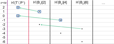
Figure 3. Spectral sequence for $T^{*}\mathbb{C}P^{1}$

Example 7.3.

$T^{*}\mathcal{B}_{p}\rightarrow\overline{\mathcal{O}_{p_{+}^{*}}}.$

The first three columns are $H^{*}(S(T^{*}\mathcal{B}_{p}))$ shifted down by $d=\dim_{\mathbb{R}}\mathcal{B}_{p}$, $2d$ and $3d$. Only the first two can hit the 0-th column via iterated differentials. The second column can hit only $H^{0}(T^{*}\mathcal{B}_{p})$. As $H^{*}(S(T^{*}\mathcal{B}_{p}))$ has no mid-degree classes, rows $0$ and $-1$ of the first column are zero, so no class in it can hit $1\in H^{0}(T^{*}\mathcal{B}_{p}),$ thus it gets killed by the second column. Altogether, the filtration is

(70) $$0\subset H^{\geq 2}(T^{*}\mathcal{B}_{p})\subset H^{*}(T^{*}\mathcal{B}_{p}).$$

For example, for the decomposition $p=(1,n)$ of $n+1$, we have $\mathcal{B}_{p}=\mathbb{C}\mathbb{P}^{n}$, $p_{+}^{*}=(2,1,1,\ldots,1)$ (with $n-1$ copies of $1$), and (69) becomes $T^{*}\mathbb{C}\mathbb{P}^{n}\rightarrow\overline{\mathcal{O}_{21\dots 1}}=\{A\in\mathfrak{sl}_{n+1}\mid A^{2}=0,\ \text{rk}(A)=1\}$, and the filtration is $0\subset H^{\geq 2}(\mathbb{C}\mathbb{P}^{n})\subset H^{*}(\mathbb{C}\mathbb{P}^{n})\cong H^{*}(T^{*}\mathbb{C}\mathbb{P}^{n})$.

Remark 7.4.

Repeating the argument verbatim, the same filtration (70) holds for Springer resolutions of any type, so $T^{*}(G/P),$ for $G$ reductive and $P$ parabolic. We discussed type A here, as we later consider Slodowy varieties of type A, in Section 7.3. Notice also that the filtration (70) is a consequence of 6.16, but we compute it here directly for the readers’ convenience.

In order to get filtrations finer than (70) on the cohomology of a flag variety, we can compose the action $\varphi$ that contracts the fibres of $T^{*}\mathcal{B}_{p}$ with a 1-parameter subgroup $G=(G_{t})_{t\in\mathbb{C}^{*}}$ of the maximal torus $T\leq GL(n,\mathbb{C}),$ as it induces a holomorphic $\mathbb{C}^{*}$-action on $T^{*}\mathcal{B}_{p}$ that commutes with $\varphi.$ The subgroups $G\leq T$ form a lattice isomorphic to $\mathbb{Z}^{n},$ via the map

$$h=(h_{1},\dots,h_{n})\in\mathbb{Z}^{n}\mapsto t^{h}:=\text{diag}(t^{h_{1}},\dots,t^{h_{n}})\leq T.$$

However, to keep the composition of $\varphi$ and $G$ contracting, it reduces the choice to a finite convex subset of this lattice. More precisely, fixing an integer $s>0$ there is a finite convex subset

$$K_{s}:=\{h\mid t^{h}\varphi^{s}\text{ is a contracting action on }T^{*}\mathcal{B}_{p}\}\subset\mathbb{Z}^{n}.$$

It is not hard to prove that $K_{1}=\emptyset$, $K_{s}\subset K_{s^{\prime}}$ for $s<s^{\prime}$ and $\cup_{s}K_{s}=\mathbb{Z}^{n}.$ Moreover, we obtain:

Proposition 7.5.

Given any integer $s>0,$ there is a map

$$K_{s}\rightarrow\{\text{filtrations of }H^{*}(\mathcal{B}_{p})\text{ by cup-ideals}\},\ h\mapsto\mathscr{F}_{\lambda}^{t^{h}\varphi^{s}}.$$

Example 7.6.

$T^{*}\mathbb{C}P^{n-1}\rightarrow\overline{\mathcal{O}_{21\dots 1}}$, with a twisted action. (See Figure 4)

Let $h=(0,1,\dots,n-1).$ The action $t^{h}\varphi^{n}|_{\mathbb{C}P^{n-1}}=t^{h}\curvearrowright\mathbb{C}P^{n-1}$ is $[z_{0},tz_{1},\dots,t^{n-1}z_{n-1}].$ The fixed points are $\mathfrak{F}_{i}:=[0,\dots,1,\dots,0],\ i=0,\dots,n-1,$ where $1$ is in the $i$-th position. There is a $(t\rightarrow\infty)$ $\mathbb{C}^{*}$-flowline from $\mathfrak{F}_{i}$ to $\mathfrak{F}_{j}$ if and only if $i<j,$ and it is $\mathbb{Z}/(j-i)$-torsion. This way we get the weight decompositions of $\mathfrak{F}_{i}$ in $\mathbb{C}P^{n-1}.$ For example, the weights of $\mathfrak{F}_{n-1}$ are $(-1,-2,\dots,-(n-1)).$ To get the full decompositions in $T^{*}\mathbb{C}P^{n-1}$, we use the $\omega_{\mathbb{C}}$-pairing $H_{k}\leftrightarrow H_{n-k}$ ((36), here the action has weight $s=n$). This yields additional weights $(n+1,n+2,\dots,2n-1)$ to $\mathfrak{F}_{n-1}.$ Similarly, we deduce the weights for the other $\mathfrak{F}_{i},$ and we observe that for each integer $k\in[n+1,2n-1]$ and $i\in[k-n,n-1]$, there is a 1-dimensional $k$-weight space in $\mathfrak{F}_{i}$. Each one of them yields a $\mathbb{Z}/k$-torsion line bundle $\mathcal{H}_{k}\rightarrow\mathfrak{F}_{i}$ in $T^{*}\mathbb{C}P^{n-1},$ whose corresponding Morse–Bott submanifold is $B_{1/k,i}\cong S^{1}.$ By (64),

$$\mu(B_{1/k,i})=2(k-n-1).$$

Thus, for $c=1,\dots,n-1,$ the $c$-th column or equivalently, time$-\frac{1}{2n-c}$ column of the spectral sequence consists of $c$ copies of $H^{*}(S^{1})[2n-2-2c],$ and a certain linear combination of its $H^{1}(S^{1})$-classes is killing the $H^{2n-2c}(\mathbb{C}P^{n-1})$ class in the $0$-th column. There are no other columns between these, as $\frac{1}{n+1}<\frac{2}{2n-1}.$ Thus, these columns kill all the cohomology except for the unit $1=H^{0}(\mathfrak{F}_{0})=H^{0}(\mathbb{C}P^{n-1}),$ which due to (10) gets killed by time $t\geq\frac{1}{n-1}$ columns. In fact, a careful estimate of indices implies that it has to be killed precisely at time-$\frac{1}{n-1}.$ Altogether, the filtration on $H^{*}(T^{*}\mathbb{C}P^{n-1})=\mathbb{K}[x]/x^{n},\ |x|=2$ is

$$0\subset\mathscr{F}_{\frac{1}{2n-1}}=\langle x^{n-1}\rangle\subset\mathscr{F}_{\frac{1}{2n-2}}=\langle x^{n-2}\rangle\subset\cdots\subset\mathscr{F}_{\frac{1}{n+1}}=\langle x\rangle\subset\mathscr{F}_{\frac{1}{n-1}}=H^{*}(T^{*}\mathbb{C}P^{n-1}),$$

so the Schubert cells in $\mathbb{C}P^{n}$ are killed by certain (linear combinations of) torsion $S^{1}$-orbits. Figure 4 is the case $n=4.$ We match by blue boxes the sets of classes that are killed one from the other by the green edge-differentials (in general we do not know whether these maps are diagonalisable). The 4-star symbol is the point of local central symmetry (6.5). Asterisk signs $*$ in the shifts of some columns indicate that shifts of their connected components are different.

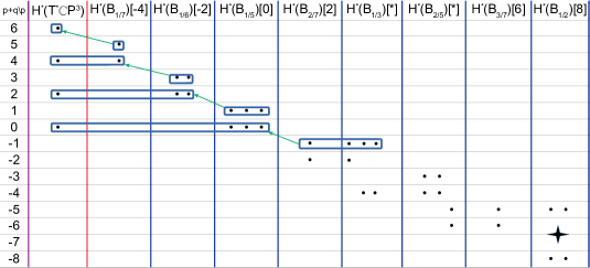
Figure 4. Spectral sequence for $T^{*}\mathbb{C}P^{3}$ with twisted action

7.2. Resolutions of ADE singularities

The CSRs of the lowest dimension are resolutions of ADE singularities. They are the minimal resolutions of quotient singularities

$$\pi_{\Gamma}:X_{\Gamma}\rightarrow\mathbb{C}^{2}/\Gamma,$$

for any finite subgroup $\Gamma\leq SL(2,\mathbb{C}).$ Such groups $\Gamma$ (up to conjugation) are in bijection with ADE Dynkin graphs $Q_{\Gamma}$. This McKay graph $Q_{\Gamma}$ encodes representation-theoretic properties of $\Gamma$. The core $\pi_{\Gamma}^{-1}(0)$ is a union of 2-spheres intersecting transversely according to $Q_{\Gamma}$. Any $\mathbb{C}^{*}$-action on $X_{\Gamma}$ preserving the core will induce a $\mathbb{C}^{*}$-action on each sphere, so the intersection points of those spheres must lie in the fixed locus $\mathfrak{F}$. The Dynkin graph $A_{n}$ corresponds to the cyclic group $\mathbb{Z}/(n+1)$; the graph $D_{n}$ corresponds to the binary dihedral group $BD_{4(n-2)}$; the graphs $E_{6},E_{7}$ and $E_{8}$ correspond to the binary tetrahedral, octahedral and icosahedral groups.

Klein showed that the coordinate ring $\mathbb{C}[\mathbb{C}^{2}/\Gamma]=\mathbb{C}[\mathbb{C}^{2}]^{\Gamma}$ is generated by three polynomials, hence the variety $\mathbb{C}^{2}/\Gamma$ embeds into $\mathbb{C}^{3}$ via a polynomial map $(z_{1},z_{2})\mapsto(f,g,h)\subset\mathbb{C}^{3}$ (see e.g. [Dol07, Sec.1.2]). Using $(X,Y,Z)$ as coordinates on $\mathbb{C}^{3}$, the embeddings for types A and D are:

(71) $$\Gamma=\mathbb{Z}/n:\ \ \ (z_{1},z_{2})\mapsto(z_{1}^{n},z_{2}^{n},z_{1}z_{2}),\text{the image is }XY-Z^{n}=0,$$

$$\Gamma=BD_{4n}:\ (z_{1},z_{2})\mapsto((z_{1}^{2n}-z_{2}^{2n})z_{1}z_{2},z_{1}^{2n}+z_{2}^{2n},z_{1}^{2}z_{2}^{2}),\text{the image is }X^{2}-Y^{2}Z+4Z^{n+1}=0.$$

The standard action on $X_{\Gamma}\rightarrow\mathbb{C}^{2}/\Gamma$ is induced from the dilation action $t\cdot(z_{1},z_{2})=(tz_{1},tz_{2})$ on $\mathbb{C}^{2}.$ It is a weight-2 conical action. 7.2 is the $A_{1}$-singularity, i.e. $\Gamma=\mathbb{Z}/2$ case.

We first consider type $A$. In the $\mathbb{C}^{3}$ coordinates of (71), the standard action is

$$t\cdot X=t^{k}X,\ \ \text{ }t\cdot Y=t^{k}Y,\ \ \text{ }t\cdot Z=t^{2}Z.$$

The torsion subvarieties are the (complex) lines $l_{1}=(0,Y,0)$ and $l_{2}=(X,0,0),$ which have $\mathbb{Z}/k$-isotropy. The torsion submanifolds in $X_{\mathbb{Z}/k}$ are the two $\mathbb{Z}/k$-torsion lines, $\widetilde{l_{1}}$ and $\widetilde{l_{2}}$ that converge to the two outer fixed points of the core. For $p=-1,\dots,-(k-1)$, the intersections $B_{p,i}=\widetilde{l}_{i}\cap\Sigma_{p}$ with each slice $\Sigma_{p}$ yields two Morse–Bott submanifolds

$$B_{p,1}\cong B_{p,2}\cong S^{1}.$$

By Lemma 6.12, the hypersurface $B_{k}$ has $H^{*}(B_{k})\cong H^{*}(S^{3}/(\mathbb{Z}/k))\cong H^{*}(S^{3})\cong\mathbb{K}_{0}\oplus\mathbb{K}_{3}.$ As the core of $X_{\Gamma}$ is an $A_{k-1}$-tree of 2-spheres, $H^{*}(X_{\Gamma})=\mathbb{K}_{0}\oplus\mathbb{K}_{2}^{k-1}.$ To compute the shifts $\mu(B_{p,i})$ we consider the weight decomposition at the two outer fixed points. The weight decomposition at any fixed point is $\mathbb{C}_{k}\oplus\mathbb{C}_{2-k},$ for some $k$, due to the duality $H_{k}\xleftrightarrow{\omega_{\mathbb{C}}}H_{2-k}$ induced by the weight-2 action. The next step depends on the parity of $k$.

Example 7.7.

$\Gamma=\mathbb{Z}/k,$ for odd $k\geq 3$. ($A_{k-1}$-singularity)

For this parity, $\tfrac{k-1}{2}$ is an integer, and by (64) the shifts are:

$$\mu(B_{p,1})=\mu(B_{p,2})=1-\mathbb{W}(\tfrac{-p}{k}k)-\mathbb{W}(\tfrac{-p}{k}(2-k))=1+\mathbb{W}(\tfrac{2p}{k})=\begin{cases*}-2,&$p<-\frac{k-1}{2},$\\ 0,&$p\geq-\frac{k-1}{2}.$\end{cases*}$$

Hence, the first $\frac{k-1}{2}$ columns of $E_{1}$ consist of two copies of $H^{*}(S^{1})$; the next $\frac{k-1}{2}$ columns consist of two copies of $H^{*}(S^{1})$ shifted down by 2; the next column is $H^{*}(S^{3}/(\mathbb{Z}/k))\cong H^{*}(S^{3})$ shifted down by $2\mu=s\cdot\dim_{\mathbb{C}}X_{\Gamma}=2\cdot 2=4$. The classes $H^{2}(X_{\Gamma})$ in the 0-th column will vanish two by two at each page, and by 6.11(2) the unit $1\in H^{0}(X_{\Gamma})$ gets killed precisely by time-1 column, thus vanishes on page $E_{k+1}$. The filtration is rank-wise

(72) $$0\ \subset\ \mathbb{K}_{2}^{2}\ \subset\ \mathbb{K}_{2}^{4}\ \subset\cdots\ \subset\ \mathbb{K}_{2}^{k-1}\ \subset\ \mathbb{K}_{0}\oplus\mathbb{K}_{2}^{k-1}=H^{*}(X_{\mathbb{Z}/k}).$$

Figure 5 shows the spectral sequence for $k=5.$

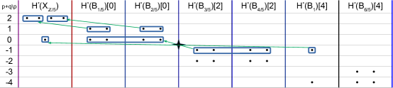
Figure 5. Spectral sequence for $X_{\mathbb{Z}/5}$

Example 7.8.

$\Gamma=\mathbb{Z}/k,$ for even $k\geq 2$. ($A_{k-1}$-singularity)

This time the action is even. By considering its square-root of weight-1, the time-$1$ column of the $E_{1}$-page is $H^{*}(\Sigma_{p})[2],$ and later columns repeat with shift $2\cdot 1=2$. The classes in $H^{2}(X_{\Gamma})$ vanish two by two until the last one is hit by the top class of the time-$1$ column, and $1\in H^{0}(X_{\Gamma})$ is killed by time-$2$ column (thus vanishes on page $E_{k+1}$) due to 6.11(1). The filtration is rank-wise

$$0\ \subset\ \mathbb{K}_{2}^{2}\ \subset\ \mathbb{K}_{2}^{4}\ \subset\cdots\ \subset\ \mathbb{K}_{2}^{k-2}\ \subset\ \mathbb{K}_{2}^{k-1}\ \subset\ \mathbb{K}_{0}\oplus\mathbb{K}_{2}^{k-1}=H^{*}(X_{\mathbb{Z}/k}).$$

Figure 6 shows the spectral sequence for $k=6.$

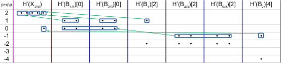
Figure 6. Spectral sequence for $X_{\mathbb{Z}/6}$

Example 7.9.

$\Gamma=\mathbb{Z}/3,$ with a non-standard action. ($A_{2}$-singularity)

We consider the non-standard weight-$2$ action induced by

$$t\cdot X=tX,\text{ }t\cdot Y=t^{2}Y,\text{ }t\cdot Z=tZ.$$

Here, there is only a $\mathbb{Z}/2$-torsion line $l_{1}=(0,Y,0).$ Its resolution $\widetilde{l_{1}}$ is a $\mathbb{Z}/2$-torsion line that converges to a fixed point $\mathfrak{F}_{1}$ with weight decomposition $\mathbb{C}_{2}\oplus\mathbb{C}_{-1}.$ By (64) the shift of the Morse–Bott submanifold $B_{1/2}=\widetilde{l_{1}}\cap\Sigma_{1}$ is $\mu(B_{1/2})=0.$ The time-1 column has shift $\mu(B_{1})=-2.$ The later columns we get by periodicity (6.4). As in the previous example, the unit gets killed by $H^{top}(B_{2})$.

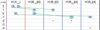
Figure 7. Spectral sequence for $X_{\mathbb{Z}/3}$ with a non-standard action.

The spectral sequence is shown on Figure 7. From it, we obtain the filtration (rank-wise)

$$0\ \subset\ \mathscr{F}_{1/2}=\mathbb{K}_{2}\ \subset\ \mathfrak{F}_{1}=\mathbb{K}_{2}^{2}\ \subset\ \mathfrak{F}_{2}=\mathbb{K}_{0}\oplus\mathbb{K}_{2}^{2}=H^{*}(X_{\mathbb{Z}/3}),$$

and together with Equation 10 we get $\mathscr{F}_{1/2}=H^{0}(\mathfrak{F}_{1})[2]=[S_{2}^{2}]$ which determines the filtration completely

$$0\ \subset\ \mathscr{F}_{1/2}=[S_{2}^{2}]\ \subset\ \mathscr{F}_{1}=\mathbb{K}_{2}^{2}\ \subset\ \mathscr{F}_{2}=\mathbb{K}_{0}\oplus\mathbb{K}_{2}^{2}=H^{*}(X_{\mathbb{Z}/3}),$$

which is different from the filtration obtained by the standard action in Example 7.7, for $k=3$:

$$0\ \subset\ \mathscr{F}_{1/3}=\mathbb{K}_{2}^{2}\ \subset\ \mathscr{F}_{1}=\mathbb{K}_{0}\oplus\mathbb{K}_{2}^{2}=H^{*}(X_{\mathbb{Z}/3}).$$

So these yield two different Floer-theoretic presentations of the ordinary cohomology of $X_{\mathbb{Z}/3},$ and determine two different filtrations by ideals on $H^{*}(X_{\mathbb{Z}/3})$.

Now consider type D. The standard action on a $D_{n+2}$-singularity, in the $\mathbb{C}^{3}$ coordinates of (71), is $t\cdot X=t^{2n+2}X$, $t\cdot Y=t^{2n}Y$, $t\cdot Z=t^{4}Z.$ For convenience, we will consider its weight-1 square root:

(73) $$t\cdot X=t^{n+1}X,\ \text{ }t\cdot Y=t^{n}Y,\ \text{ }t\cdot Z=t^{2}Z.$$

Example 7.10.

$\Gamma=BD_{8k}$ ($D_{2k+2}$-singularity), $k\geq 1.$ (See Figure 8)

For $n=2k$, (73) is $t\cdot X=t^{2k+1}X$, $t\cdot Y=t^{2k}Y$, $t\cdot Z=t^{2}Z.$ There are three torsion lines

$$\alpha=(0,Y,0),\ \beta_{1}=(0,2Z^{k},Z),\ \beta_{2}=(0,-2Z^{k},Z),$$

with respective torsion groups $\mathbb{Z}/2k,\mathbb{Z}/2,\mathbb{Z}/2$. As it is a weight-1 action, it has a (unique) fixed core component [Ž22], which is the sphere corresponding to the unique trivalent vertex of the graph $D_{2k+2}.$ The resolutions $\widetilde{\alpha},\widetilde{\beta_{1}},\widetilde{\beta_{2}}$ of the torsion lines $\alpha,\beta_{1},\beta_{2}$ are lines again, and they converge to the fixed points of the spheres that correspond to the leaves of the graph $D_{2k+2}$ (because these are the leaves of the attraction graph, and by Proposition 2.9 each such leaf has a torsion bundle that converges to it).

Using formula (64), as in the previous examples, one can calculate the degree shifts $\mu(B_{p,c})$ of the Morse Bott submanifolds $B_{p,c}\cong S^{1}$ which are intersections of the lines $\widetilde{\alpha},\widetilde{\beta_{1}},\widetilde{\beta_{2}}$ with the slices $\Sigma_{p}$. They all have zero shift, for $T_{p}<1.$ Then, $B_{1}=\Sigma_{1}$ has a shift down by 2 (as the action has weight 1), and the other columns are determined by Corollary 6.4. The filtration is rank-wise:

$$\text{for }k=1:\ 0\subset\mathbb{K}_{2}^{3}\subset\mathbb{K}_{2}^{4}\subset\mathbb{K}_{0}\oplus\mathbb{K}_{2}^{4}=H^{*}(X_{\Gamma}),$$

$$\text{for }k\geq 2:\ 0\subset\mathbb{K}_{2}\subset\dots\subset\mathbb{K}_{2}^{k-1}\subset\mathbb{K}_{2}^{k+2}\subset\mathbb{K}_{2}^{k+3}\dots\subset\mathbb{K}_{2}^{2k+1}\subset\mathbb{K}_{2}^{2k+2}\subset H^{*}(X_{\Gamma}).$$

In both cases, the jump in rank by $3$ occurs at the time-$\frac{1}{2}$ column, as all three lines are $\mathbb{Z}/2$-torsion.

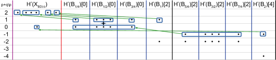
Figure 8. Spectral sequence for $D_{6}$ ($k=2$, $n=4$).

Example 7.11.

$\Gamma=BD_{8k+4}$ ($D_{2k+3}$-singularity), $k\geq 1.$ (See Figure 9)

For $n=2k+1$, (73) is $t\cdot X=t^{2k+2}X$, $t\cdot Y=t^{2k+1}Y$, $t\cdot Z=t^{2}Z.$ There are three torsion lines

$$\alpha=(0,Y,0),\ \beta_{1}=(2iZ^{k+1},0,Z),\ \beta_{2}=(-2iZ^{k+1},0,Z),$$

with respective isotropies $\mathbb{Z}/(2k+1),\mathbb{Z}/2,\mathbb{Z}/2$. Again they give rise to circles $B_{p,\beta}$ with zero shifts. The novelty now is the time $\frac{1}{2}$-column: there are two Morse–Bott submanifolds, so the filtration at time $\frac{1}{2}$ jumps by rank 2 in degree 2. Thus, the filtration is rank-wise

$$0\subset\mathbb{K}_{2}\subset\dots\subset\mathbb{K}_{2}^{k}\subset\mathbb{K}_{2}^{k+2}\subset\mathbb{K}_{2}^{k+3}\subset\dots\subset\mathbb{K}_{2}^{2k+3}\subset H^{*}(X_{\Gamma}).$$

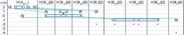
Figure 9. Spectral sequence for $D_{5}$ ($k=1$, $n=3$).

Example 7.12.

$D_{n}$ via the attraction graph. It soon becomes desirable to obtain descriptions of the Morse–Bott manifolds that avoid the coordinate presentations like (71), instead using the attraction graph (2.8). We illustrate this for $D_{n}$. The core consists of a Dynkin tree $D_{n}$, each vertex corresponds to a sphere, and each edge corresponds to an intersection of spheres which in turn is a fixed point of the action, and the sphere $C$ at the unique trivalent vertex is fixed (as it carries three fixed points). At each fixed point, $\omega_{\mathbb{C}}$-duality implies that the weight decomposition is $H_{k}\oplus H_{2-k}$, each summand having $\dim_{\mathbb{C}}=1$. If a sphere in the core is fixed, it has a weight $k=0$, thus $H_{0}\oplus H_{2}$ and the Morse–Bott index is $0$. By Equation 6 there can be only one fixed sphere, which is $C$, so the other spheres must carry exactly two fixed points (by considering the rank in Equation 6). By 2.7, it is now easy to write out the weight decompositions at all fixed points, and the attraction graph is again a $D_{n}$-Dynkin graph. It is preferable to use the square-root of the action, which exists as there is a fixed component $C$ of maximal ($\omega_{\mathbb{C}}$-Lagrangian) dimension in the core. This is based on the analytic continuation of the square-root that exists on the torsion bundle $\mathcal{H}_{2}\rightarrow C,$ see [Ž22, Lem.5.4. and Prop.5.5]. Now, as the square-root is a weight-1 conical action, $\omega_{\mathbb{C}}$-duality gives $H_{k}\oplus H_{1-k}$ decompositions. We have $H_{0}\oplus H_{1}$ at $C$, e.g. at intersections points $p_{1},p_{2},p_{3}$ with the adjacent spheres $C_{1},C_{2},C_{3}$; at the second fixed points $q_{1},q_{2},q_{3}$ of $C_{1},C_{2},C_{3}$ we get $H_{-1}\oplus H_{2}$ by 2.7 ($C_{i}$ defines a $\mathbb{C}^{*}$-flow from $p_{i}$ to $q_{i}$). For $D_{4}$, the $q_{i}$ are leaf nodes in the attraction graph, and their $H_{2}$ defines a $\mathbb{Z}/2$-torsion line bundle $\mathcal{H}_{2}$, yielding Morse–Bott manifolds $S^{1}$ when intersecting with slices. For $D_{n}$ with $n>4$, the same applies to two of those $q_{i}$. The third corresponds to where additional edges arise in the $D_{n}$ Dynkin diagram: they correspond to fixed points with $H_{-2}\oplus H_{3}$, $H_{-3}\oplus H_{4}$, $\ldots$, $H_{-(n-3)}\oplus H_{n-2},$ yielding a $\mathbb{Z}/(n-2)$-torsion line bundle at the leaf (and so again $S^{1}$ Morse–Bott manifolds). So we recover Examples 7.10 and 7.11 without needing (71).

Example 7.13.

$E_{6}$, $E_{7}$, $E_{8}$ Singularities. (See Figure 11)

We use the method from 7.12, as the previous method that uses the invariant polynomials becomes too complicated. The core for $E_{6}$ is the $E_{6}$-Dynkin tree of spheres, and the sphere $C$ that corresponds to the trivalent node of $E_{6}$ is fixed. Thus, like in the previous example, the standard action has a square-root, which is a weight-1 conical action, and its weight decomposition at $C$ is $H_{0}\oplus H_{1}.$ The attraction graph is an $E_{6}$ Dynkin diagram. We get a $\mathbb{Z}/2$-torsion and two $\mathbb{Z}/3$-torsion line bundles over fixed points that correspond to the leaves, Figure 10.

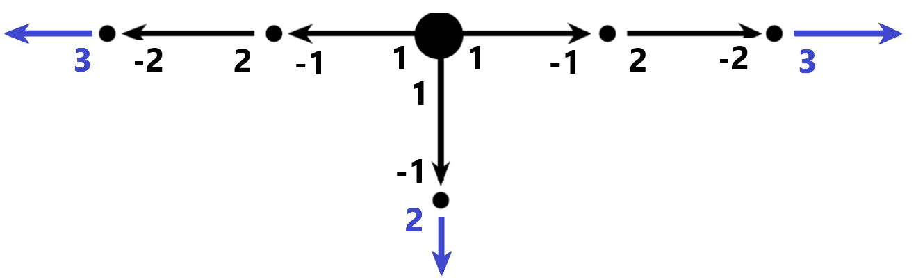
Figure 10. $E_{6}$-singularity: extended attraction graph of the minimal resolution.

Thus, the Morse–Bott submanifolds are circles, and their shifts are calculated in the usual way from the weight decompositions $H_{-1}\oplus H_{2}$, $H_{-2}\oplus H_{3}$, $H_{-2}\oplus H_{3}$ of their converging points.

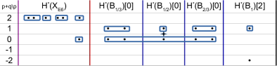
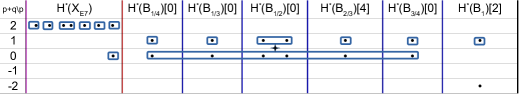
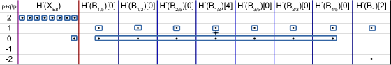
Figure 11. Spectral sequence for $E_{6}$, $E_{7}$, $E_{8}$ (omitting edge-differentials for readability)

The three torsion line bundles over fixed points at leaves of the attraction graph for $E_{6}$ were $\mathbb{Z}/2$, $\mathbb{Z}/3$, $\mathbb{Z}/3$; for $E_{7}$ this becomes $\mathbb{Z}/2$, $\mathbb{Z}/3$, $\mathbb{Z}/4$; for $E_{8}$: $\mathbb{Z}/2,\mathbb{Z}/3,$ $\mathbb{Z}/5.$ The filtrations are:

$$\small\begin{split}E_{6}:&\;0\subset\mathbb{K}_{2}^{2}\subset\mathbb{K}_{2}^{3}\subset\mathbb{K}_{2}^{5}\subset\mathbb{K}_{2}^{6}\subset\mathbb{K}_{0}\oplus\mathbb{K}_{2}^{6}=H^{*}(X_{\Gamma}).\\ E_{7}:&\;0\subset\mathbb{K}_{2}\subset\mathbb{K}_{2}^{2}\subset\mathbb{K}_{2}^{4}\subset\mathbb{K}_{2}^{5}\subset\mathbb{K}_{2}^{6}\subset\mathbb{K}_{2}^{7}\subset\mathbb{K}_{0}\oplus\mathbb{K}_{2}^{7}=H^{*}(X_{\Gamma}).\\ E_{8}:&\;0\subset\mathbb{K}_{2}\subset\mathbb{K}_{2}^{2}\subset\mathbb{K}_{2}^{3}\subset\dots\subset\mathbb{K}_{2}^{7}\subset\mathbb{K}_{2}^{8}\subset\mathbb{K}_{0}\oplus\mathbb{K}_{2}^{8}=H^{*}(X_{\Gamma}).\end{split}$$

7.3. Slodowy varieties of type A

We will now consider resolutions of ordinary Slodowy varieties of type A, with the Kazhdan $\mathbb{C}^{*}$-action. Recall that the nilpotent cone $\mathcal{N}$ of the Lie algebra $\mathfrak{sl}_{n}$ is the variety of all nilpotent matrices, and it has an associated (ordinary) Springer resolution,

(74) $$\nu:\widetilde{\mathcal{N}}\rightarrow\mathcal{N},\ \{(e,F=(0=F_{0}\subset F_{1}\subset\dots\subset F_{n-1}\subset F_{n}=\mathbb{C}^{n}))\mid eF_{i}\subset F_{i-1}\}\mapsto e,$$

which is a special case of the map (69), when $p=(1,\dots,1),$ as then $\mathcal{N}=\overline{\mathcal{O}_{n}}.$ Recall $\widetilde{\mathcal{N}}\cong T^{*}\mathcal{B},$ where $\mathcal{B}=\mathcal{B}_{1\dots 1}$ is the ordinary flag variety in $\mathbb{C}^{n}.$ The fibres of the map (74) are called Springer fibres. It is a standard fact that they are equidimensional projective varieties, whose irreducible components are labelled bijectively by Standard Young Tableaux of the shape that corresponds to the Jordan partition of the nilpotent matrix, [Spa76]. Given a nilpotent matrix $e\in\mathcal{N},$ by the Jacobson-Morozov theorem there is an $\mathfrak{sl}_{2}$-triple $(e,f,h)$ of nilpotent matrices. Choosing such a triple, one constructs the Slodowy slice

$$S_{e}=\{x\in\mathfrak{sl}_{n}\mid[x-e,f]=0\}=e+\text{ker}(\text{ad}f).$$

The Slodowy variety and its resolution are defined as $\mathcal{S}_{e}:=S_{e}\cap\mathcal{N},$ $\widetilde{\mathcal{S}}_{e}:=\nu^{-1}(\mathcal{S}_{e}).$ On the Slodowy slice and Slodowy variety, the Kazhdan action is $t\cdot x=t^{2}\text{Ad}(t^{-h})x.$ Its lift to $\widetilde{\mathcal{S}}_{e}$ is given by

(75) $$t\cdot(x,F)=(t^{2}\mathrm{Ad}(t^{-h})x,t^{-h}F).$$

The map $\nu:\widetilde{\mathcal{S}}_{e}\rightarrow\SS_{e}$ is a weight-2 CSR with that action. Its core is the Springer fibre $\mathcal{B}^{e}=\nu^{-1}(e).$ Picking a Jordan basis $(v_{i})$ for the triple $(e,f,h),$ that action on a matrix $x=(X_{ij})$ becomes

(76) $$t\cdot(X_{ij})=(t^{2+h_{j}-h_{i}}X_{ij}),$$

whereas the action on flags is induced by the action on $\mathbb{C}^{n}$ given by

(77) $$t\cdot v_{i}=t^{-h_{i}}v_{i},$$

where $h=\text{diag}(h_{1},\dots,h_{n})$ in the basis $v_{i}.$ Given a partition $\lambda=(\lambda_{1},\dots,\lambda_{k}),$ we will use the nilpotent element $e_{\lambda}:=\text{diag}(J_{\lambda_{1}},\dots,J_{\lambda_{k}})$ given by the standard Jordan canonical form for the partition $\lambda$ (so $\lambda_{i}\times\lambda_{i}$ Jordan blocks with eigenvalue zero). There is a choice of an $\mathfrak{sl}_{2}$-triple $(e_{\lambda},f_{\lambda},h_{\lambda})$ such that they have the same Jordan basis and $h_{\lambda}$ becomes diagonal in this basis. One can also explicitly compute the corresponding Slodowy slice $S_{\lambda}:=S_{e_{\lambda}}.$ For the details of this, see [Ž20, Sec.5.2.1-5.2.2], in particular [Ž20, Prop.5.2.14.] for the description for $S_{\lambda}.$ One additional observation that we prove here is

Lemma 7.14.

The fixed points of the Kazhdan action on $\widetilde{\mathcal{S}}_{\lambda}$ are isolated, or equivalently, its corresponding $S^{1}$-moment map is Morse if $\lambda=(m,n),$ and $m\neq n\ \mathrm{(mod\ 2)}.$

Proof.

From the description of $h_{\lambda}$ given in [Ž20, p.112], it is clear that if $\lambda=(m,n),$ $m\neq n\ \mathrm{(mod\ 2)},$ then $h_{\lambda}$ has distinct entries (explicitly: $h_{\lambda}=(m-1,m-3,\dots,-(m-1),n-1,n-3,\dots,-(n-1))$). Thus there is no Kazhdan-invariant subspace on $\mathbb{C}^{n},$ and all fixed flags on $\mathcal{B}$ are isolated. Now recall that fixed points in $\widetilde{\mathcal{S}}_{\lambda}$ are contained in its core, which is $\mathcal{B}^{\lambda}\subset\mathcal{B}.$ ∎

The basic algorithm we use is that we first find the torsion points $\{\mathcal{T}_{\mathbb{Z}/{m}}\}_{m\geq 2}$ in the Slodowy slice $S_{\lambda},$ then we restrict to the nilpotent cone $\mathcal{N}$ in order to get the torsion points

$$\mathcal{P}_{\mathbb{Z}/{m}}:=\mathcal{T}_{\mathbb{Z}/{m}}\cap\mathcal{N}$$

in the Slodowy variety $\mathcal{S}_{\lambda}.$ Then, using the Springer resolution $\nu$, we find the corresponding torsion points in $\widetilde{\mathcal{S}}_{\lambda}=\nu^{-1}(\mathcal{S}_{\lambda}),$ denoted by $\{\mathcal{R}_{\mathbb{Z}/{m}}\}_{m\geq 2}.$ As the fibres of the resolution $\nu$ depend on the nilpotent orbit $\mathcal{O}_{\gamma}$ where they are taken, we will keep track of $\gamma$ in the intersections

$$\mathcal{P}_{\mathbb{Z}/{m,\gamma}}:=\mathcal{T}_{\mathbb{Z}/{m}}\cap\mathcal{O}_{\gamma},\ \ \mathcal{P}_{\mathbb{Z}/{m}}=\sqcup_{\gamma}\mathcal{P}_{\mathbb{Z}/{m,\gamma}}.$$

In addition, when the Kazhdan action is even, we will consider a square-root of it, in order to avoid all points trivially being $\mathbb{Z}/2$-torsion. We will use the notation $B_{T_{p}}$ instead of $B_{p}$ for the Morse–Bott submanifolds, so that it agrees with the spectral sequence labelling.

Example 7.15.

Slodowy variety $\mathcal{S}_{22}.$ For $\lambda=(2,2)$, $n=4,$ using [Ž20, Prop.5.2.14.] one gets the description of the Slodowy slice $S_{22}$ in $\mathfrak{sl}_{4}$ at the nilpotent element $e_{22}=\text{diag}(J_{2},J_{2}).$ In particular, $h_{22}=\text{diag}(1,-1,1,-1).$

$$\small S_{22}=\left\{\begin{bmatrix}a&1&c&0\\ m&a&p&c\\ e&0&-a&1\\ x&e&w&-a\end{bmatrix}\middle|\ a,c,e,m,p,x,w\in\mathbb{C}\right\}.$$

As $t^{h_{22}}=diag(t,t^{-1},t,t^{-1})$, by formula (76) the Kazhdan action on $S_{22}$ is

(78) $$\small t\cdot\begin{bmatrix}a&1&c&0\\ m&a&p&c\\ e&0&-a&1\\ x&e&w&-a\end{bmatrix}=\begin{bmatrix}t^{2}a&1&t^{2}c&0\\ t^{4}m&t^{2}a&t^{4}p&t^{2}c\\ t^{2}e&0&-t^{2}a&1\\ t^{4}x&t^{2}e&t^{4}w&-t^{2}a\end{bmatrix}.$$

Thus, we see that the action is even, so we take a square root of it. Then, we only have powers $t^{1}$ and $t^{2}$ of $t$ in equation (78), hence we get only $\mathbb{Z}/2$-torsion points in $S_{22},$

$$\small\mathcal{T}_{\mathbb{Z}/{2}}=\left\{\begin{bmatrix}0&1&0&0\\ m&0&p&0\\ 0&0&0&1\\ x&0&w&0\end{bmatrix}\middle|m,p,x\in\mathbb{C}\right\}.$$

Intersecting it with the nilpotent cone $\mathcal{N}=\{A\mid A^{4}=0\},$ after some amount of computations one gets the set of $\mathbb{Z}/2$-torsion points in Slodowy variety $\mathcal{S}_{22}:$

(79) $$\small\mathcal{P}_{\mathbb{Z}/{2}}=\left\{\begin{bmatrix}0&1&0&0\\ m&0&p&0\\ 0&0&0&1\\ x&0&w&0\end{bmatrix}\middle|\ m^{2}+px=0,\ m,p,x\in\mathbb{C}\right\}\cong\mathbb{C}^{2}/(\mathbb{Z}/2).$$

One can check that these matrices, except for the zero matrix, all lie in the regular orbit $\mathcal{O}_{4},$ hence are bijectively lifted to $\widetilde{\mathcal{S}}_{22}$ under the Springer resolution. Denoting by $A_{mpx}$ the matrix in equation (79), for $(m,p,x)\neq(0,0,0),$ its lift is the Springer fibre $(A_{mpx},F_{mpx}).$ Thus the flag

$$F_{mpx}=(0\subset F_{1}\subset F_{2}\subset F_{3}\subset\mathbb{C}^{4})$$

is defined by $A_{mpx}F_{i}\subset F_{i-1}.$ Let $(v_{1},v_{2},v_{3},v_{4})$ be the basis in which these matrices are given. Then

$$F_{mpx} =(0\subset\langle pv_{1}-mv_{3}\rangle\subset\langle pv_{1}-mv_{3},pv_{2}-mv_{4}\rangle\subset\langle v_{1},v_{3},pv_{2}-mv_{4}\rangle\subset\mathbb{C}^{4}),\text{when }(p,m)\neq(0,0),$$

$$F_{mpx} =(0\subset\langle mv_{1}+xv_{3}\rangle\subset\langle mv_{1}+xv_{3},mv_{2}+xv_{4}\rangle\subset\langle v_{1},v_{3},mv_{2}+xv_{4}\rangle\subset\mathbb{C}^{4}),\text{when }(m,x)\neq(0,0).$$

Using (77), we see that the Kazhdan action acts on $\mathbb{C}^{n}$ by

$$t\cdot(v_{1},v_{2},v_{3},v_{4})=(t^{-1}v_{1},tv_{2},t^{-1}v_{3},tv_{4}),$$

thus the induced action makes the flag $F_{mpx}$ fixed. Hence, the fixed locus to which $\mathcal{R}_{\mathbb{Z}/{2}}$ converges (when $t\rightarrow 0$) is a ${\mathbb{P}}^{1}$ in the core:

$$\mathfrak{F}_{mpx}:=(0\subset\langle\alpha v_{1}+\beta v_{3}\rangle\subset\langle\alpha v_{1}+\beta v_{3},\alpha v_{2}+\beta v_{4}\rangle\subset\langle v_{1},v_{3},\alpha v_{2}+\beta v_{4}\rangle\subset\mathbb{C}^{4}\mid[\alpha:\beta]\in{\mathbb{P}}^{1}).$$

Thus, $\mathcal{R}_{\mathbb{Z}/{2}}$ has a single connected component, which is a torsion bundle $\mathcal{R}_{\mathbb{Z}/{2}}=\mathcal{H}_{2}\rightarrow\mathfrak{F}_{mpx}.$ Being a resolution of the cone $\mathcal{P}_{\mathbb{Z}/{2}}\cong\mathbb{C}^{2}/(\mathbb{Z}/2),$ it is a $A_{1}$ singularity resolution, hence $\mathcal{H}_{2}\cong T^{*}\mathbb{C}P^{1}.$ So, the cohomology of its hypersurface $B_{1/2}=\mathcal{S}_{1/2}\cap\mathcal{H}_{2}$ is isomorphic to the cohomology of the unit bundle $S(T^{*}\mathbb{C}P^{1})\cong\mathbb{R}P^{3},$ by 6.12. As we work over the field $\mathbb{K}$ of characteristic zero,

$$H^{*}(B_{1/2})\cong H^{*}(\mathbb{R}P^{3})=\mathbb{K}_{0}\oplus\mathbb{K}_{3}.$$

The cohomology of the space $\widetilde{\mathcal{S}}_{22}$ is isomorphic to the cohomology of its core, the Springer fibre $\mathcal{B}^{22}.$ Vector space generators of $H^{*}(\mathcal{B}^{\lambda})$ are labelled by row-standard tableaux of shape $\lambda,$ and the degrees of the generators can be easily computed by some tableaux combinatorics [Fre09, Sec.1.3]. Using the prescribed method therein, one obtains

$$H^{*}(\widetilde{\mathcal{S}}_{22})\cong H^{*}(\mathcal{B}^{22})\cong\mathbb{K}_{0}\oplus\mathbb{K}_{2}^{3}\oplus\mathbb{K}_{4}^{2}.$$

Thus, from 6.14 and 6.15 one obtains the cohomology of the slice. We now find the degree shifts. As the weight decomposition of $\mathfrak{F}_{mpx}$ has $H_{0}\oplus H_{2}$ as a summand, by $\omega_{\mathbb{C}}$-duality it also has $H_{1-2}=H_{-1}$ and $H_{1-0}=H_{1}$ (recall we square-rooted the action so $\omega_{\mathbb{C}}$ has weight 1). Thus we have $T_{\mathfrak{F}_{mpx}}\widetilde{\mathcal{S}}_{22}=H_{-1}\oplus H_{0}\oplus H_{1}\oplus H_{2},$ and then by (64) we find $\mu(B_{1/2})=0.$ By 6.11(1), the unit is killed by the top class of the time-2 column. We obtain Figure 12, where we crop at the mid-dimensional cohomology of the time-$2$ slice. Thus, the rank-wise filtration on $H^{*}(\widetilde{\mathcal{S}}_{22})$ is

(80) $$0\subset\mathbb{K}_{4}\subset\mathbb{K}_{2}^{3}\oplus\mathbb{K}_{4}^{2}\subset\mathbb{K}_{0}\oplus\mathbb{K}_{2}^{3}\oplus\mathbb{K}_{4}^{2}=H^{*}(\widetilde{\mathcal{S}}_{22}).$$

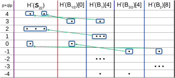
Figure 12. Spectral sequence for $\mathcal{S}_{22}$

Moreover, using Equation 10 we get that $\mathscr{F}_{1/2}=H^{2}(\mathfrak{F}_{mpx})[2]$, since here we have only two fixed components (due to 2.19(12)), the other one being $\mathfrak{F}_{min}$. In the Atiyah–Bott decomposition $H^{*}(\widetilde{\mathcal{S}}_{22})=H^{*}(\mathfrak{F}_{\min})\oplus H^{*}(\mathfrak{F}_{mpx})[-2]$, the class $H^{2}(\mathfrak{F}_{mpx})[-2]=[\overline{\mathfrak{L}_{mpx}}]$ corresponds to the class of the irreducible core component $\overline{\mathfrak{L}_{mpx}}$ arising as the closure of the downward flow from $\mathfrak{F}_{mpx}$. In the Springer-theoretic notation, this irreducible component is labelled $\overline{\mathfrak{L}_{mpx}}=\mathcal{K}_{T}$ by the standard Young tableaux $T=\ytableau 1&2\\ 34$ and $\mathfrak{F}_{min}=\mathcal{K}_{T^{\prime}}$ is labelled by $T^{\prime}=\ytableau 1&3\\ 24$. Thus, we get the complete description:

(81) $$0\subset\mathscr{F}_{1/2}=[\mathcal{K}_{T}]\subset\mathscr{F}_{1}=\mathbb{K}_{2}^{3}\oplus\mathbb{K}_{4}^{2}\subset\mathscr{F}_{2}=\mathbb{K}_{0}\oplus\mathbb{K}_{2}^{3}\oplus\mathbb{K}_{4}^{2}=H^{*}(\widetilde{\mathcal{S}}_{22}).$$

Example 7.16.

Slodowy variety $\mathcal{S}_{32}.$ For $\lambda=(3,2)$, $n=5,$ as before one computes the slice $S_{32}:$

$$\small S_{32}=\left\{\begin{bmatrix}2a&1&0&0&0\\ f&2a&1&j&0\\ l&f&2a&p&2j\\ 2y&0&0&-3a&1\\ w&y&0&x&-3a\end{bmatrix}\middle|\ a,f,j,l,p,x,y,w\in\mathbb{C}\right\}.$$

and $h_{32}=\text{diag}(2,0,-2,1,-1).$ As $t^{h_{32}}=\text{diag}(t^{2},t^{0},t^{-2},t^{1},t^{-1}),$ the Kazhdan action on $S_{32}$ by (76) is

$$\small t\cdot\begin{bmatrix}2a&1&0&0&0\\ f&2a&1&j&0\\ l&f&2a&p&2j\\ 2y&0&0&-3a&1\\ w&y&0&x&-3a\end{bmatrix}=\begin{bmatrix}2t^{2}a&1&0&0&0\\ t^{4}f&2t^{2}a&1&t^{3}j&0\\ t^{6}l&t^{4}f&2t^{2}a&t^{5}p&2t^{3}j\\ 2t^{3}y&0&0&-3t^{2}a&1\\ t^{5}w&t^{3}y&0&t^{4}x&-3t^{2}a\end{bmatrix}.$$

Thus, we see that $S_{32}$ has $\mathbb{Z}/k$-torsion points for all $k=2,3,4,5,6.$ Restricting to $\SS_{32}=\{A\in S_{32}\mid A^{5}=0\},$ some matrix calculations by computer show that only $\mathbb{Z}/3$ and $\mathbb{Z}/5$-torsion points remain on it. Explicitly (where in lower indices we label the coordinates used on $\mathbb{C}^{2}$ and $\mathbb{C}$):

(82) $$\small\mathcal{P}_{\mathbb{Z}/{3}}=\left\{A_{jy}:=\begin{bmatrix}0&1&0&0&0\\ 0&0&1&j&0\\ -5jy&0&0&0&2j\\ 2y&0&0&0&1\\ 0&y&0&0&0\end{bmatrix}\middle|\ j,y\in\mathbb{C}\right\}\cong\mathbb{C}^{2}_{j,y},$$

(83) $$\small\mathcal{P}_{\mathbb{Z}/{5}}=\left\{A_{pw}:=\begin{bmatrix}0&1&0&0&0\\ 0&0&1&0&0\\ 0&0&0&p&0\\ 0&0&0&0&1\\ w&0&0&0&0\end{bmatrix}\middle|\ pw=0\right\}\cong\mathbb{C}_{p}\cup\mathbb{C}_{w},$$

$\mathbb{Z}/5$ torsion points: Apart from the zero matrix, $\mathcal{P}_{\mathbb{Z}/{5}}$ lies in the regular orbit $\mathcal{O}_{5}.$ Therefore it is bijectively lifted to $\widetilde{\mathcal{S}}_{32}$ under the Springer resolution, to pairs $(A_{p0},F_{p})$ and $(A_{0w},F_{w})$ where

$$F_{p}:=(0\subset\langle v_{1}\rangle\subset\langle v_{1},v_{2}\rangle\subset\langle v_{1},v_{2},v_{3}\rangle\subset\langle v_{1},v_{2},v_{3},v_{4}\rangle\subset\mathbb{C}^{5})$$

$$F_{w}:=(0\subset\langle v_{4}\rangle\subset\langle v_{4},v_{5}\rangle\subset\langle v_{1},v_{4},v_{5}\rangle\subset\langle v_{1},v_{2},v_{4},v_{5}\rangle\subset\mathbb{C}^{5})$$

as one can easily compute from the Springer fibre conditions $A_{0w}F_{w}\subset F_{w},\ A_{p0}F_{p}\subset F_{p}.$ Here, $(v_{1},v_{2},v_{3},v_{4})$ is the basis in which the matrices are given. In the limit $t\rightarrow 0$ of the Kazhdan action,

$$\lim_{t\rightarrow 0}t\cdot(A_{p0},F_{p})=(e_{32},F_{p}),\ \ \ \lim_{t\rightarrow 0}t\cdot(A_{0w},F_{w})=(e_{32},F_{w})$$

hence, these two $\mathbb{Z}/5$-torsion lines converge to two points $F_{p}$ and $F_{w}$ in the Springer fibre $\mathcal{B}^{32}.$ They yield two Morse–Bott submanifolds

$$B_{1/5}=B_{1/5,1}\sqcup B_{1/5,2}\cong S^{1}\sqcup S^{1},$$

but we cannot compute the shifts $\mu(B_{1/5,i})$ yet, as we lack information on the weight decomposition at $\mathscr{F}_{p}$ and $\mathscr{F}_{w}$ in the core $\mathcal{B}^{32}.$ We will be able to do it after considering the $\mathbb{Z}/3$-torsion points.

$\mathbb{Z}/3$ torsion points: By checking for which $j,y\in\mathbb{C}$ we have $A_{jy}^{4}=0,$ we find that in $\mathcal{P}_{\mathbb{Z}/{3}}$ the two lines $j=0$ and $y=0$ lie on the subregular orbit $\mathcal{O}_{41},$ whereas the rest lie in $\mathcal{O}_{5}.$ Thus, for $j,y\neq 0$ the fibre above $A_{jy}$ is $(A_{jy},F_{jy})$ where, after some computation,

$$F_{jy}=(0\subset\langle jv_{3}-v_{4}\rangle\subset\langle jv_{3}-v_{4},v_{1}+yv_{5}\rangle\subset\langle jv_{3}-v_{4},v_{1}+yv_{5},v_{2}\rangle\subset\langle v_{2},v_{3},v_{4},v_{1}+yv_{5}\rangle\subset\mathbb{C}^{5}).$$

This flag also makes sense for $j=0$ or $y=0,$ and due to continuity, we get a slice

$$S_{jy}=\{(A_{jy},F_{jy})\mid j,y\in\mathbb{C}\}\cong\mathbb{C}^{2}.$$

By (77), the Kazhdan action acts on $\mathbb{C}^{n}$ by $t\cdot(v_{1},v_{2},v_{3},v_{4},v_{5})=(t^{-2}v_{1},v_{2},t^{2}v_{3},t^{-1}v_{4},tv_{5}),$ thus one immediately gets $\displaystyle\lim_{t\rightarrow 0}t\cdot(A_{jy},F_{jy})=(e_{32},F_{big}),$ where

$$F_{big}:=(0\subset\langle v_{4}\rangle\subset\langle v_{1},v_{4}\rangle\subset\langle v_{1},v_{2},v_{4}\rangle\subset\langle v_{1},v_{2},v_{3},v_{4}\rangle\subset\mathbb{C}^{5}).$$

Thus the whole slice $S_{jy}$ converges to the flag $F_{big},$ yielding a trivial rank 2 torsion bundle $\mathcal{H}_{3}\rightarrow F_{big}.$ The corresponding Morse–Bott submanifold $B_{1/3,big}$ is cohomologically isomorphic to the sphere bundle

(84) $$H^{*}(B_{1/3,big})\cong H^{*}(S(\mathcal{H}_{3}))\cong H^{*}(S^{3})=\mathbb{K}_{0}\oplus\mathbb{K}_{3},$$

and knowing the weight decomposition $H_{3}\oplus H_{3}\oplus H_{-1}\oplus H_{-1}$ of $F_{big}$ we also compute $\mu(B_{1/3,big})=0.$

Now let us consider the $\mathbb{Z}/3$-torsion points in the fibre over $A_{j0},$ where $j\neq 0.$ The Springer fibre over $A_{j0}$ is a Dynkin $A_{4}$-tree of spheres ${\mathbb{P}}_{1}^{1}\cup{\mathbb{P}}_{2}^{1}\cup{\mathbb{P}}_{3}^{1}\cup{\mathbb{P}}_{4}^{1}$ that intersect transversally. Standard computations from Springer theory yield their explicit flag description:

$${\mathbb{P}}_{1}^{1}[\alpha:\beta]= (0\subset\langle\alpha v_{1}+\beta(\tfrac{1}{j}v_{4}-v_{3})\rangle\subset\langle v_{1},\tfrac{1}{j}v_{4}-v_{3}\rangle\subset\langle v_{1},v_{2},\tfrac{1}{j}v_{4}-v_{3}\rangle\subset\langle v_{1},v_{2},v_{3},v_{4}\rangle\subset\mathbb{C}^{5})$$

$${\mathbb{P}}_{2}^{1}[\alpha:\beta]= (0\subset\langle v_{1}\rangle\subset\langle v_{1},\alpha v_{2}+\beta(\tfrac{1}{j}v_{4}-v_{3})\rangle\subset\langle v_{1},v_{2},\tfrac{1}{j}v_{4}-v_{3}\rangle\subset\langle v_{1},v_{2},v_{3},v_{4}\rangle\subset\mathbb{C}^{5})$$

$${\mathbb{P}}_{3}^{1}[\alpha:\beta]= (0\subset\langle v_{1}\rangle\subset\langle v_{1},v_{2}\rangle\subset\langle v_{1},v_{2},\alpha v_{3}+\beta\tfrac{1}{j}v_{4}\rangle\subset\langle v_{1},v_{2},v_{3},v_{4}\rangle\subset\mathbb{C}^{5})$$

$${\mathbb{P}}_{4}^{1}[\alpha:\beta]= (0\subset\langle v_{1}\rangle\subset\langle v_{1},v_{2}\rangle\subset\langle v_{1},v_{2},2v_{3}+\tfrac{1}{j}v_{4}\rangle\subset\langle v_{1},v_{2},2v_{3}+\tfrac{1}{j}v_{4},\alpha v_{3}+\beta\tfrac{1}{j}v_{5}\rangle\subset\mathbb{C}^{5})$$

Recall that the Kazhdan action is $t\cdot(v_{1},v_{2},v_{3},v_{4},v_{5})=(t^{-2}v_{1},v_{2},t^{2}v_{3},t^{-1}v_{4},tv_{5}),$ which for the primitive third root of unity $\varepsilon$ gives

$$\varepsilon\cdot(v_{1},v_{2},v_{3},v_{4},v_{5})=(\varepsilon v_{1},v_{2},\varepsilon^{-1}v_{3},\varepsilon^{-1}v_{4},\varepsilon v_{5}).$$

Notice that the $\mathbb{Z}/3$-torsion points in the fibre are exactly the flags fixed by the $\varepsilon$ action. Thus, we get that the $\mathbb{Z}/3$-torsion points in the Springer fibre above $A_{j0}$ are

$${\mathbb{P}}_{1}^{1}[0:1],\ \ {\mathbb{P}}_{1}^{1}[1:0],\ \ {\mathbb{P}}_{3}^{1}[\alpha:\beta],\ \ {\mathbb{P}}_{4}^{1}[0:1],$$

so three points and a sphere. Note the point ${\mathbb{P}}_{1}^{1}[0:1]=F_{j0}$ is already contained in the slice $S_{jy}.$ One computes directly that $\displaystyle\lim_{t\rightarrow 0}t\cdot(A_{j0},{\mathbb{P}}_{1}^{1}[1:0])=(e_{32},F_{j}^{3}),$ and $\displaystyle\lim_{t\rightarrow 0}t\cdot(A_{j0},{\mathbb{P}}_{4}^{1}[0:1])=(e_{32},F_{j}^{1}),$ where

$$F_{j}^{3}:=(0\subset\langle v_{1}\rangle\subset\langle v_{1},v_{4}\rangle\subset\langle v_{1},v_{2},v_{4}\rangle\subset\langle v_{1},v_{2},v_{3},v_{4}\rangle\subset\mathbb{C}^{5})$$

$$F_{j}^{1}:=(0\subset\langle v_{1}\rangle\subset\langle v_{1},v_{2}\rangle\subset\langle v_{1},v_{2},v_{4}\rangle\subset\langle v_{1},v_{2},v_{4},v_{5}\rangle\subset\mathbb{C}^{5}).$$

Thus, these two yield $\mathbb{Z}/3$-torsion line bundles over the points $F_{j}^{3}$ and $F_{j}^{1}.$ Hence, their Morse–Bott submanifolds are circles,

$$B_{1/3,j^{3}}\cong B_{1/3,j^{1}}\cong S^{1}.$$

The convergence (under Kazhdan action and $t\rightarrow 0$) of the spheres

(85) $$\small{\mathbb{P}}_{3}^{1}[\alpha:\beta]_{j}=(0\subset\langle v_{1}\rangle\subset\langle v_{1},v_{2}\rangle\subset\langle v_{1},v_{2},\alpha v_{3}+\beta\tfrac{1}{j}v_{4}\rangle\subset\langle v_{1},v_{2},v_{3},v_{4}\rangle\subset\mathbb{C}^{5}\mid[\alpha:\beta]\in{\mathbb{P}}^{1})$$

is a bit more involved. Namely, (85) converges to

$$F_{p}= (0\subset\langle v_{1}\rangle\subset\langle v_{1},v_{2}\rangle\subset\langle v_{1},v_{2},v_{3}\rangle\subset\langle v_{1},v_{2},v_{3},v_{4}\rangle\subset\mathbb{C}^{5}),\text{when }\beta=0$$

$$F_{j}^{\prime}:= (0\subset\langle v_{1}\rangle\subset\langle v_{1},v_{2}\rangle\subset\langle v_{1},v_{2},v_{4}\rangle\subset\langle v_{1},v_{2},v_{3},v_{4}\rangle\subset\mathbb{C}^{5}),\text{otherwise.}$$

Notice also that there is a $\mathbb{Z}/3$-torsion sphere in the core between these two points:

$$C_{jp}=\{(0\subset\langle v_{1}\rangle\subset\langle v_{1},v_{2}\rangle\subset\langle v_{1},v_{2},\alpha v_{3}+\beta v_{4}\rangle\subset\langle v_{1},v_{2},v_{3},v_{4}\rangle\subset\mathbb{C}^{5})\mid[\alpha:\beta]\in{\mathbb{P}}^{1}\}.$$

Thus, altogether with ${\mathbb{P}}_{3}^{1}[\alpha:\beta]$ we get a $\mathbb{Z}/3$-torsion line bundle over the (non-fixed) sphere $C_{jp}:$

$$\{(A_{j0},F)\mid j\in\mathbb{C}\}\mapsto F\in C_{jp}.$$

This bundle is trivial, and by Lemma 6.12 the corresponding Morse–Bott submanifold $B_{1/3,jp}$ is cohomologically isomorphic to its sphere bundle,

(86) $$H^{*}(B_{1/3,jp})\cong H^{*}(S^{2}\times S^{1})\cong\mathbb{K}_{0}\oplus\mathbb{K}_{1}\oplus\mathbb{K}_{2}\oplus\mathbb{K}_{3}.$$

The weight-decomposition of $F_{j}^{\prime}$ is $H_{3}\oplus H_{3}\oplus H_{-1}\oplus H_{-1},$ thus by formula (64) one computes the grading $\mu(B_{1/3,jp})=0.$ Now we compute the gradings of the Morse–Bott submanifolds $B_{1/3,j^{3}}$ and $B_{1/3,j^{1}}.$ We claim that the weight-decompositions of their corresponding fixed loci $F_{j}^{3}$ and $F_{j}^{1}$ are both

(87) $$H_{3}\oplus H_{-1}\oplus H_{1}\oplus H_{1},$$

due to the following accumulative argument. Assuming the contrary and that there is a weight-space $H_{2},$ it then yields a $\mathbb{C}^{*}$-flowline in the core (as there are no $\mathbb{Z}/2$-torsion points outside of the core) which converges to another fixed set to weight-space $H_{-2}$ (2.7). Thus, by $\omega_{\mathbb{C}}$-duality, that fixed set has an $H_{4}$ weight-space, which again yields a $\mathbb{C}^{*}$-orbit etc. As the number of components of the fixed locus is finite, this process must stop and we get a contradiction. The same would happen if we had assumed that there was a weight-space $H_{k\geq 4}$ in $F_{j}^{3}$ and $F_{j}^{1}.$ Otherwise, assume that $H_{3}$ is 2-dimensional. That would mean that there are more outer $\mathbb{Z}/3$-torsion points converging to $F_{j}^{3}$ and $F_{j}^{1},$ so again, a contradiction. Thus the weight-decompositions (87) hold, and by (64) we get

$$\mu(B_{1/3,j^{3}})=\mu(B_{1/3,j^{1}})=0.$$

Completely analogously, considering $A_{0y}$ and its fibres we get (cohomologically) the same Morse–Bott submanifolds together with the same gradings. Also, we get analogous fixed points $F_{y}^{3},F_{y}^{1},F_{y}^{\prime}.$

Similarly to the last example, by counting the row-standard Young tableaux of shape $(3,2)$ with grading defined in [Fre09, Sec.1.3] we get the ordinary cohomology

$$H^{*}(\widetilde{\mathcal{S}}_{32})\cong H^{*}(\mathcal{B}^{32})\cong\mathbb{K}_{0}\oplus\mathbb{K}_{2}^{4}\oplus\mathbb{K}_{4}^{5}.$$

Observe Figure 13. At time-$\frac{2}{3}$ column, the four copies of $S^{1}$ have shift 2 whereas $S^{3}$ and the two $S^{2}\times S^{1}$ have shift 4, hence we use (as before) the asterisk notation to denote mixed shifts. By 6.11(2), $1\in H^{0}(\widetilde{\mathcal{S}}_{32})$ is killed by the top class of the time-1 column. The filtration is

(88) $$0\ \subset\ \mathscr{F}_{1/5}=\mathbb{K}_{4}^{2}\ \subset\ \mathscr{F}_{1/3}=\mathbb{K}_{2}^{r}\oplus\mathbb{K}_{4}^{5}\subset\mathscr{F}_{2/5}=\mathbb{K}_{2}^{4}\oplus\mathbb{K}_{4}^{5}\subset\ \mathscr{F}_{1}=\mathbb{K}_{0}\oplus\mathbb{K}_{2}^{4}\oplus\mathbb{K}_{4}^{5}=H^{*}(\widetilde{\mathcal{S}}_{32}),$$

where $r\in\{2,3,4\}$ remains unknown, due to potential vertical differentials in column $B_{1/3}$.

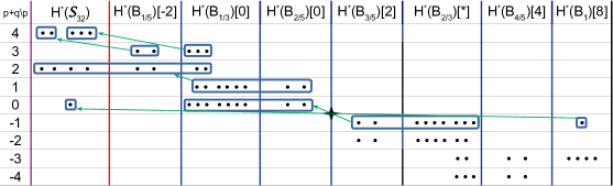
Figure 13. Spectral sequence for $\mathcal{S}_{32}$

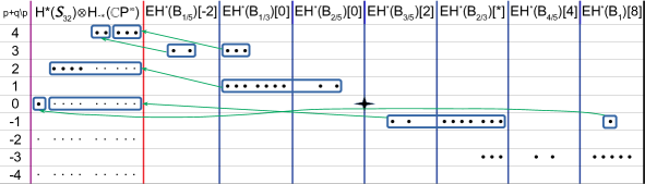
Figure 14. $S^{1}$-Equivariant spectral sequence for $\mathcal{S}_{32}$

Example 7.17.

Slodowy variety $\mathcal{S}_{32},$ using the $S^{1}$-equivariant spectral sequence.

Figure 14 shows the $S^{1}$-equivariant spectral sequence for $ESH^{*}(Y,\varphi)$. The $0$-th column $H^{*}(Y;\mathbb{K})\otimes_{\mathbb{K}}\mathbb{F}$ consists of copies of the $\mathbb{K}[u]$-module $\mathbb{F}=\mathbb{K}(\!(u)\!)/u\mathbb{K}[\![u]\!]\cong H_{-*}(\mathbb{C}{\mathbb{P}}^{\infty})$ mentioned in Section 1.8: the larger dots correspond to the $u^{0}$-part, and the smaller dots correspond to the $u^{-j}$-copies of that generator for $j\geq 1$. This example illustrates 1.31 (and one can see explicitly how 1.33 arises in practice).

The edge-differentials preserve the $u$-action, but unfortunately the $u$-action has been mostly forgotten once we pass to the $E_{1}$-page. The first three dots in degree $1$ for the $B_{1/3}$-column have a non-trivial vertical $u$-action (see 1.8), so they must hit $u^{<0}$-classes in the $0$-th column. However, the other four dots in degree $1$ for the $B_{1/3}$-column may have non-trivial $u$-action hitting the $B_{1/5}$-column, so in principle we only know that at least two of the first four dots in the $0$-th column in degree 2 (which are $u^{0}$-terms) get killed. This ambiguity is precisely the unknown value $r\in\{2,3,4\}$ in (88).

Remark 7.18.

Equation 9 and 5.16 can also be used to deduce information about the cohomology of fixed components $\mathfrak{F}_{\alpha}$ from the spectral sequence. The $0$-th column in Figure 13 has a total rank of $10$, and this rank must persist as we add new columns provided we take into account all the green arrows. So if we consider the block given by all columns $p$ whose periods $T_{p}$ are below a certain slope, we must get total rank $10$. By Corollary 9 the degrees in which these ranks live will shift in complicated ways, as we increase the slope. Observing how the gradings shift can reveal information about the cohomology of individual fixed components $\mathfrak{F}_{\alpha}$. In Figure 13 an extreme example occurs: if we consider all columns up to $B_{2/5}$, we see that all of the rank $10$ is supported in degree $0$. By Equation 9, that means each $\mathfrak{F}_{\alpha}$ has cohomology supported in just one degree, so each $\mathfrak{F}_{\alpha}$ is a point. So $\mathfrak{F}={\widetilde{\mathcal{S}}_{32}}^{\mathbb{C}^{*}}$ consists of 10 points. Alternatively, this follows from 7.14.

Example 7.19.

Slodowy varieties $\mathcal{S}_{211},\mathcal{S}_{311},\mathcal{S}_{33},\mathcal{S}_{42}.$

In addition, we show the spectral sequences $E(\varphi)^{pq}_{r}$ for $\mathcal{S}_{211}$ and $\mathcal{S}_{311}$ (Figure 15), $\mathcal{S}_{33}$ (Figure 16) and $\mathcal{S}_{42}$ (Figure 17), that we obtain analogously to previous examples. For convenience, we denote the cohomology ranks of the $B_{1}/B_{2}$ in some entries by a number rather than by black dots. As before, from them one can read-off the filtrations on ordinary cohomology (rank-wise).

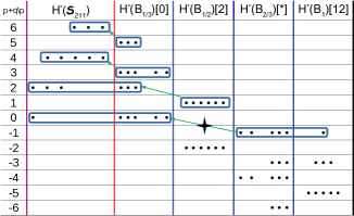
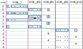
Figure 15. Spectral sequences for $\mathcal{S}_{211}$ and $\mathcal{S}_{311}$

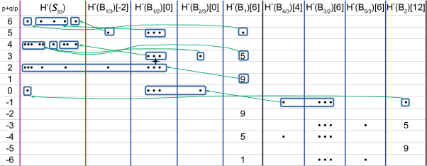
Figure 16. Spectral sequence for $\mathcal{S}_{33}$

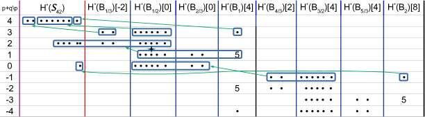
Figure 17. Spectral sequence for $\mathcal{S}_{42}$

7.4. Moduli of Higgs bundles

The last class of examples that we consider are moduli spaces of Higgs bundles. They come with a hyperkähler structure $(\mathcal{M},I,J,K,g)$ and a canonical $I$-holomorphic $\mathbb{C}^{*}$-action $\varphi$ that acts with weight-1 on the holomorphic symplectic form

(89) $$t\cdot\omega_{\mathbb{C}}=t\omega_{\mathbb{C}},\ \omega_{\mathbb{C}}:=\omega_{I}+i\omega_{J}$$

and the $S^{1}$-part preserves the Kähler form $\omega_{I}.$ There is a proper holomorphic map, the Hitchin fibration,

$$\Psi:\mathcal{M}\to B\cong\mathbb{C}^{\frac{1}{2}\dim_{\mathbb{C}}\mathcal{M}},$$

equivariant w.r.t. a certain linear action on the base. $(\mathcal{M},\omega_{I})$ is a symplectic $\mathbb{C}^{*}$-manifold globally defined over the convex base $B$ via $\Psi.$ Given $G\in\{GL(n,\mathbb{C}),\ SL(n,\mathbb{C})\},$ $d\in\mathbb{N}_{0}$ coprime to $n,$ consider $\mathcal{M}_{G}(d,g),$ the moduli of $G$-Higgs bundles of degree $d$ over a Riemann surface of genus $g\geq 2.$

Proposition 7.20.

[RŽ23a] $Q_{\varphi}=0$ for $\mathcal{M}_{G}(d,g),$ so $\mathscr{F}_{1}^{\varphi}=H^{*}(\mathcal{M}_{G}(d,g)).$

Example 7.21.

$G=GL(1,\mathbb{C}),$ $\mathcal{M}_{G}(d,g)\cong T^{*}T^{2g}.$

For $G=GL(1,\mathbb{C}),$ the moduli space is the cotangent bundle of the torus $T^{2g}$ (for $SL(1,\mathbb{C})$ it is a point), with the standard weight-1 $\mathbb{C}^{*}$-action on fibres. The Maslov index is $\mu=\frac{1}{2}\dim_{\mathbb{C}}\mathcal{M}=g,$ and the columns in the spectral sequence (after the 0-column) are cohomologies of the sphere bundle $H^{*}(B_{k})=H^{*}(S^{*}T^{2g})$ shifted by $2g,4g,6g,\dots.$ Due to the Gysin sequence and $\chi(T^{2g})=0,$ we get $H^{*}(B_{k})\cong H^{*}(T^{2g})\otimes H^{*}(S^{2g-1}).$ By 7.20, the filtration is trivial,

$$\mathscr{F}^{\varphi}_{0}=0\subset H^{*}(\mathcal{M}_{GL(1,\mathbb{C})}(d,g))=\mathscr{F}^{\varphi}_{1}.$$

Interestingly, one cannot conclude this just by looking at the spectral sequence itself (see Figure 18, left). The unit $1\in H^{0}(\mathcal{M})$ could in principle be killed by $H^{top}(B_{2}),$ but the triviality of the intersection form (used in the proof of 7.20) prevents this. Thus the unit gets killed by a mid-degree class from the time-1 column (lower yellow box in Figure 18). This is very different from CSRs, whose intersection form is non-degenerate, and mid-degrees in the time-1 column vanish, so differentials from $H^{top}(B_{2})$ can hit the unit $1\in H^{0}(\mathcal{M})$ (e.g. Figure 3).

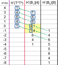
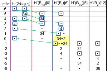
Figure 18. Spectral sequence for $GL(1,\mathbb{C})$ and $SL(2,\mathbb{C})$ Higgs moduli over $g=2$

Example 7.22.

$G=SL(2,\mathbb{C}),$ $g=2.$

The topology of Higgs moduli for $G=SL(2,\mathbb{C})$ are well-understood. The $\mathbb{C}^{*}$-fixed locus is completely described [Hit87, Prop.7.1]. For $g=2$ we have two fixed components, $\mathfrak{F}_{0}=\mathfrak{F}_{\min}$ and $\mathfrak{F}_{1}$,

$$H^{*}(\mathfrak{F}_{0})\cong\mathbb{K}_{0}\oplus\mathbb{K}_{2}\oplus\mathbb{K}_{3}^{4}\oplus\mathbb{K}_{4}\oplus\mathbb{K}_{6},\ \ \ \ H^{*}(\mathfrak{F}_{1})\cong\mathbb{K}_{0}\oplus\mathbb{K}_{1}^{34}\oplus\mathbb{K}_{2},$$

with Morse–Bott indices $\mu_{0}=0$, $\mu_{1}=4.$ The attraction graph is quite simple: by $\omega_{\mathbb{C}}$-duality, there are only $H_{0}$ and $H_{1}$ weight spaces at $\mathfrak{F}_{0},$ so there is a weight-1 flow from $\mathfrak{F}_{0}$ to $\mathfrak{F}_{1},$ creating a $H_{-1}$ weight space at $\mathfrak{F}_{1}.$ Due to the Morse–Bott index, $H_{-1}$ is 2-dimensional. By $\omega_{\mathbb{C}}$-duality, there is 2-dimensional $H_{2},$ creating a torsion bundle $\mathcal{H}_{2}\rightarrow\mathfrak{F}_{1}$ of rank 2. Thus, the associated Morse–Bott manifold has

$$H^{*}(B_{1/2})\cong H^{*}(S\mathcal{H}_{2})\cong H^{*}(S^{3})\otimes H^{*}(\mathfrak{F}_{1})\cong\mathbb{K}_{0}\oplus\mathbb{K}_{1}^{34}\oplus\mathbb{K}_{2}\oplus\mathbb{K}_{3}\oplus\mathbb{K}_{4}^{34}\oplus\mathbb{K}_{5}.$$

The time-1 column is computed via 6.14 and the fact that the intersection form is trivial, by Hausel [Hau98]. The spectral sequence (see Figure 18, right) yields the filtration

$$0\subset\mathbb{K}_{2}^{r}\oplus\mathbb{K}_{3}^{s}\oplus\mathbb{K}_{4}\oplus\mathbb{K}_{5}^{34}\oplus\mathbb{K}_{6}\subset H^{*}(\mathcal{M}_{SL(2,\mathbb{C})}(d,2))$$

where $(r,s)\in\{0,1\}\times\{0,1\}$ remains unknown. Notice that the minimal component $\mathfrak{F}_{0}$ has only weights 0 and 1, due to weight-1 condition (89) and $\omega_{\mathbb{C}}$-duality (36). However, due to $H^{odd}(\mathfrak{F}_{0})\neq 0,$ we cannot use Equation 10, which would have given us $\mathscr{F}^{\varphi}_{1/2}\subset H^{*}(\mathfrak{F}_{1})[-4],$ hence $r=s=0.$

Example 7.23.

Parabolic Higgs bundles of $\dim_{\mathbb{C}}=2.$

One can also consider moduli of so-called parabolic Higgs bundles, where we add marked points to the Riemann surface where poles of the Higgs field of certain types are allowed. All parabolic Higgs moduli in the lowest complex dimension $2$ are given as crepant resolutions

(90) $$\pi:\mathcal{M}_{\Gamma}\rightarrow(T^{*}E)/\Gamma,$$

where $E$ is an elliptic curve, and $\Gamma$ is a finite group of automorphisms of $E$, [Gro14, Zha17]. Composing $\pi$ and the projection to $\mathbb{C}$ coming from the isomorphism $T^{*}E\cong E\times\mathbb{C}$, yields the Hitchin fibration

(91) $$\Psi:\mathcal{M}_{\Gamma}\rightarrow\mathbb{C}.$$

The core of $\mathcal{M}_{\Gamma}$ is the central fibre $\Psi^{-1}(0)$ whose irreducible components are curves intersecting according to affine Dynkin graphs $Q_{\Gamma}=\widetilde{A_{0}},\ \widetilde{D_{4}},\ \widetilde{E_{6}},\ \widetilde{E_{7}},\ \widetilde{E_{8}},$ when the group $\Gamma={0},\ \mathbb{Z}/2,\ \mathbb{Z}/3,\ \mathbb{Z}/4,\ \mathbb{Z}/6,$ respectively. In particular, the case $\Gamma=\{0\}$ gives us $\mathcal{M}_{\Gamma}=T^{*}E;$ in other cases all curves are $\mathbb{C}P^{1}$s.

Similarly to Examples 7.12, 7.13, we get the spectral sequence via the attraction graph, which for the $\Gamma=\mathbb{Z}/6$ case are given in Figures 19 and 20. The $\mathbb{C}P^{1}$ corresponding to the (3+)-valent vertex of the graph is fixed, thus it is precisely the minimal component $\mathfrak{F}_{\min}$ [Ž20] of the $\mathbb{C}^{*}$-action.

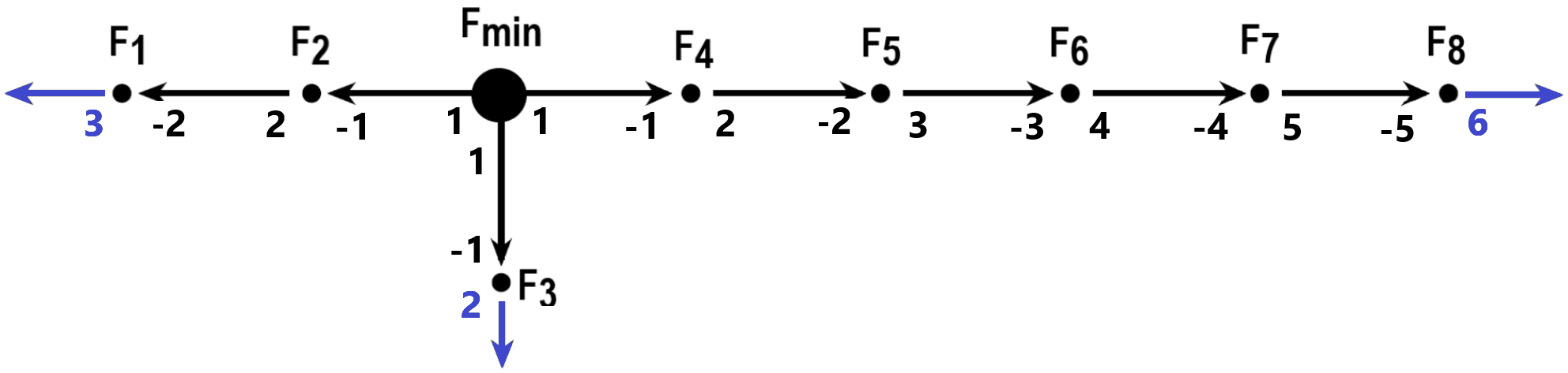
Figure 19. Extended attraction graph for $\mathcal{M}_{\mathbb{Z}/6}$

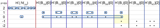
Figure 20. Spectral sequence for $\mathcal{M}_{\mathbb{Z}/6}$ ($Q=\widetilde{E_{8}}$), omitting edge-differentials

An interesting new phenomenon is that $\mathscr{F}^{\varphi}_{1}\neq H^{*}(\mathcal{M}_{\Gamma}),$ whereas the spectral sequence alone cannot prove it: the mid-cohomologies of the time-1 column (lower light-yellow box in Figure 20) could potentially kill the unit. The first observation is due to $\mathfrak{F}_{\min}\cong{\mathbb{P}}^{1}$ having non-zero Euler characteristic and the result [RŽ23a, Cor.7.28] from our previous paper. Each mid-cohomology of the time-1 column has rank 1 due to 6.14 (and Equation 68 in it), as $H^{1}(\mathcal{M}_{\Gamma})=0$ and the intersection form matrix on $H_{2}(\mathcal{M}_{\Gamma})\cong H_{2}(\Psi^{-1}(0))$ equals minus the Cartan matrix of an affine Dynkin graph $Q_{\Gamma}$, thus has 1-dimensional kernel. From the spectral sequences, we obtain $\mathscr{F}^{\varphi}_{\lambda}$ for $\mathcal{M}_{\Gamma}:$

(92) $$\small\begin{split}\widetilde{A_{0}}:&\;0\subset\mathbb{K}_{0}\oplus\mathbb{K}_{1}^{2}\oplus\mathbb{K}_{2}=H^{*}(\mathcal{M}_{\Gamma}).\\ \widetilde{D_{4}}:&\;0\subset\mathbb{K}_{2}\subset\mathbb{K}_{2}^{5}\subset\mathbb{K}_{0}\oplus\mathbb{K}_{2}^{5}=H^{*}(\mathcal{M}_{\Gamma}).\\ \widetilde{E_{6}}:&\;0\subset\mathbb{K}_{2}^{3}\subset\mathbb{K}_{2}^{6}\subset\mathbb{K}_{2}^{7}\subset\mathbb{K}_{0}\oplus\mathbb{K}_{2}^{7}=H^{*}(\mathcal{M}_{\Gamma}).\\ \widetilde{E_{7}}:&\;0\subset\mathbb{K}_{2}^{2}\subset\mathbb{K}_{2}^{5}\subset\mathbb{K}_{2}^{7}\subset\mathbb{K}_{2}^{8}\subset\mathbb{K}_{0}\oplus\mathbb{K}_{2}^{8}=H^{*}(\mathcal{M}_{\Gamma}).\\ \widetilde{E_{8}}:&\;0\subset\mathbb{K}_{2}\subset\mathbb{K}_{2}^{3}\subset\mathbb{K}_{2}^{5}\subset\mathbb{K}_{2}^{7}\subset\mathbb{K}_{2}^{8}\subset\mathbb{K}_{2}^{9}\subset\mathbb{K}_{0}\oplus\mathbb{K}_{2}^{9}=H^{*}(\mathcal{M}_{\Gamma}).\end{split}$$

Interestingly, the filtrations obtained on the $H^{2}(\mathcal{M}_{\Gamma})$ have representation-theoretic meaning, and we thank Alexandre Minets for pointing it out to us. Namely, consider the root system of the affine Dynkin graph $Q:=Q_{\Gamma}$ (where $Q^{0}$ denotes its vertices):

$$R_{Q}=\{\alpha_{i}\mid i\in Q^{0}\}\sqcup\langle\mathbb{Z}-{0}\rangle\delta.$$

It contains simple roots $\alpha_{i}$, labelled by vertices of the graph $Q,$ and multiples of the imaginary root

(93) $$\delta=\sum_{i\in{Q^{0}}}n_{i}\alpha_{i}$$

that generates the kernel of the corresponding Cartan matrix $C_{Q}.$ An example of these numbers $n_{i}$ for the graph $\widetilde{E_{8}}$ is given in Figure 21, and the others can be found in [KJ16, Fig.1.3].

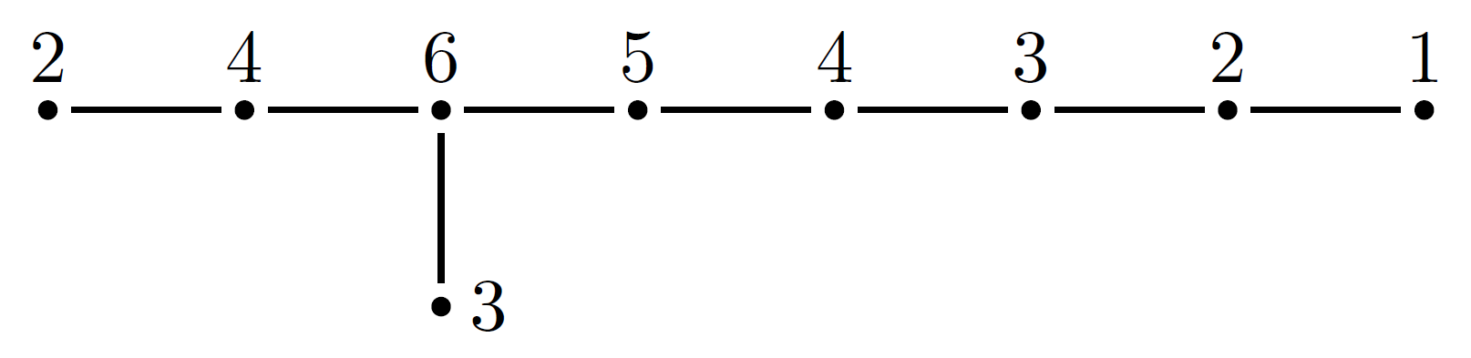
Figure 21. $\widetilde{E_{8}}$ with imaginary root labelling

The irreducible components of the core of $\mathcal{M}_{\Gamma}$ form the base for its top-cohomology $H^{2}(\mathrm{Core}(\mathcal{M}_{\Gamma}))\cong H^{2}(\mathcal{M}_{\Gamma}),$ and are labeled by $Q^{0},$ thus we have $H^{2}(\mathcal{M}_{\Gamma})=\mathbb{K}\langle Q^{0}\rangle.$ By direct comparison of (92) with the numbers $n_{i}$ from (93) we get (where $|V|$ denotes the dimension over $\mathbb{K}$):

Proposition 7.24.

Denoting by $\mathscr{F}_{k}$ the $k$-th step of the filtration $\mathscr{F}^{\varphi}_{\lambda}$ of $H^{2}(\mathcal{M}_{\Gamma}),$ we have

$\displaystyle|\mathscr{F}_{k}|=\#\{i\in Q^{0}\mid n_{i}\leq k\}.$ ∎

Let us now compare our filtration with the perverse filtration for $\Psi,$ which is proved in [Zha17] to be equal to the weight filtration of the associated character variety $\mathcal{M}_{\Gamma}^{\prime},$ confirming the famous “$P=W$” conjecture of [dCHM12] in this case. Since the two filtrations are of different type (the perverse filtration has the unit in the first filtered level, whereas in ours it is at the last level), it makes sense to compare them only degree-wise, which here amounts to considering $H^{2}(\mathcal{M}_{\Gamma})$:

Proposition 7.25.

The filtration $\mathscr{F}^{\varphi}_{\lambda}(H^{2}(\mathcal{M}_{\Gamma}))$ refines the perverse, thus $P=W$, filtration.

Proof.

In the trivial example $T^{*}E,$ the filtrations are equal, thus let us consider $\Gamma\neq\{0\}.$ The perverse filtration on $H^{2}(\mathcal{M}_{\Gamma})$ due to [Zha17, Prop.5.4] has two steps:

$$(P_{0}H^{2}(\mathcal{M}_{\Gamma})=0)\subset(P_{1}H^{2}(\mathcal{M}_{\Gamma})=\langle[E_{i}]\mid i\rangle)\subset(P_{2}H^{2}(\mathcal{M}_{\Gamma})=H^{2}(\mathcal{M}_{\Gamma}))$$

where $E_{i}$ are the exceptional divisors of (90), which are the components of the core $\Psi^{-1}(0)$ except the minimal component $\mathfrak{F}_{\min}$ corresponding to the (3+)-valent vertex $c$ of Dynkin graph $Q.$ As $\mathfrak{F}_{min}$ is fixed, its weight decomposition is $H_{0}\oplus H_{1}$, due to $\omega_{\mathbb{C}}$-duality (36) for the weight-1 action (89). Thus, by Equation 10, the penultimate filtered level is

(94) $$\mathscr{F}^{\varphi}_{1^{-}}(H^{2}(\mathcal{M}_{\Gamma}))=\oplus_{i}H^{0}(\mathfrak{F}_{i})[-2],$$

where $\mathfrak{F}_{i}$ are the other fixed points, labelled bijectively by $i\in Q^{0}\setminus\{c\}$ via their $(t\rightarrow\infty)$-flow: $E_{i}=\overline{\mathfrak{L}_{i}},$ where $\mathfrak{L}_{i}:=\{p\mid\lim_{t\rightarrow\infty}t\cdot p=\mathfrak{F}_{i}\}.$ Since the classes in the Atiyah–Bott decomposition (94) correspond to the classes $[E_{i}]$ of their downward flows, we conclude that $\mathscr{F}^{\varphi}_{1^{-}}(H^{2}(\mathcal{M}_{\Gamma})=\langle[E_{i}]\rangle=P_{1}H^{2}(\mathcal{M}_{\Gamma}).$ ∎

Appendix A Morse–Bott–Floer complex and cascades

A.1. Cascades, drops and ledges: the Morse–Bott–Floer complex

We refer the reader to Bourgeois–Oancea and Frauenfelder [BO09a, BO09b, Fra04] for the original implementations of this construction, and also to the applications thereof in [KvK16, App.B] and [MR23, App.E].

The arguments in this section are quite general, so $(Y,\omega)$ will denote a symplectic manifold for which Hamiltonian Floer cohomology and continuation maps can be defined for a suitable class of “admissible” Hamiltonians. For example, closed symplectic manifolds, or Liouville manifolds using Hamiltonians radial at infinity, or symplectic $\mathbb{C}^{*}$-manifolds $Y$ over a convex base using admissible Hamiltonians as in [RŽ23a]. We fix an $\omega$-compatible almost complex structure $I$ on $Y$, and we use the Riemannian metric $\omega(\cdot,I\cdot)$ when defining gradients and Morse flowlines.

Call $H:Y\to\mathbb{R}$ a Morse–Bott–Floer Hamiltonian if it is an admissible Hamiltonian whose $1$-orbits consist of finitely many closed connected submanifolds $B_{i}\subset Y$ (these parametrise the initial points of the $1$-orbits) and $B_{i}$ is Morse–Bott for $H$, which is the condition from 5.6:

(95) $$T_{y}B_{i}=\mathrm{Ker}\,(d\varphi^{1}_{H}-\mathrm{id})|_{y}\textrm{ for all }y\in B_{i}.$$

Equivalently, the intersection of the graph of $\varphi^{1}_{H}$ in $(Y\times Y,\omega\oplus-\omega)$ with the diagonal is a clean intersection (of two Lagrangian submanifolds) and equals the diagonal of $B_{i}$. One can also allow $H$ to be time-dependent. Given a Morse–Bott–Floer Hamiltonian $H$, we choose auxiliary Morse functions $f_{i}:B_{i}\to\mathbb{R}$. Simplify notation further by denoting $B=\sqcup_{i}B_{i}=\mathrm{Crit}(H)$, and $f:B\to\mathbb{R}$ the Morse function defined by the $f_{i}$. As in Section 5.1, a point $x_{0}\in B$ corresponds to the initial point $x(0)=x_{0}$ of a $1$-orbit $x(t)$; we call it the associated $1$-orbit. If $x_{0}\in\mathrm{Crit}(f)$ is a critical point, we call $x(t)\subset Y$ a critical $1$-orbit. Thus the critical $1$-orbits are an isolated subset of the space of $1$-orbits of $H$. We will abusively blur the distinction between a critical point and its associated critical $1$-orbit.

The Morse–Bott Floer complex $BCF^{*}(H)$ is freely generated over the Novikov field $\mathbb{K}$ by the critical $1$-orbits, equivalently (by blurring the above distinction) the generators are the subset $\mathrm{Crit}(f)\subset B$ of critical points. As usual, there are various possible choices of $\mathbb{K}$ depending on the setup (Section 2.3); this is not important in our discussion. The differential on $BCF^{*}(H)$ is a count of isolated cascades, which we define below, yielding a cohomology group $BHF^{*}(H)$. When we say “count”, we always mean an oriented count, with weights depending on the choice of $\mathbb{K}$. Often $\mathbb{K}$ involves a variable $T$ to encode energy, and the “weight” means $T^{E(u)}$ where $E(u)$ is the energy of the cascade in B.1.

The discussion of orientation signs is rather subtle [BO09b, Prop.3.9]. Bourgeois–Oancea [BO09b, Sec.4.4] discussed these in detail when the Morse–Bott manifolds are circles. Kwon – van Koert [KvK16, Lem.B.7] studied orientations in detail for the local Floer cohomology of a class of Morse–Bott manifolds satisfying a certain symplectic triviality condition. We suggest a general construction of orientation signs in LABEL:Section_{\MBF}_theory:_orientations assuming only that $c_{1}(Y)=0$, building on Appendices B–C.

In general, only when $c_{1}(Y)=0$ there is a well-defined $\mathbb{Z}$-grading on $BCF^{*}(H)$ (rather than just a $\mathbb{Z}/2$ grading), with $T$ lying in degree zero. The grading of the critical $1$-orbits uses the conventions of [MR23, App.C] explained in Section 2.4: for a critical $1$-orbit $x$ associated to $x_{0}\in\mathrm{Crit}(f_{i})\subset B_{i}$,

(96) $$|x|:=\mu_{f_{i}}(x_{0})+\mu_{H}(B_{i})=\mu_{f_{i}}(x_{0})+\dim_{\mathbb{C}}\,Y-\tfrac{1}{2}\dim_{\mathbb{R}}B_{i}-RS(B_{i},H),$$

where $\mu_{f_{i}}$ is the Morse index, and $RS(B_{i},H)=RS(x,H)$ is the Robbin–Salamon index of $x$ (which only depends on the connected Morse–Bott manifold $B_{i}$). The motivation for this grading follows from the proof of C.9.

A ledge is any flowline of $-\nabla f$ inside $B$ (using the Riemannian metric on $B$ restricted from $Y$). We say the ledge is modelled on an interval $\mathrm{Int}\subset\mathbb{R}\cup\{\pm\infty\}$ if the flowline is a map $\mathrm{Int}\to B$ (which will land in some component $B_{i}\subset B$). We say that a Floer solution is non-trivial if it has strictly positive energy, $E(u)=\int\|\partial_{s}u\|^{2}\,ds\wedge dt>0$. Trivial Floer trajectories have zero energy, so $\partial_{t}u-X_{H}=0$, so $t\mapsto u(s,t)$ is an $s$-independent $1$-orbit; we will prohibit these inside cascades. A drop is any non-trivial Floer trajectory $u:\mathbb{R}\times S^{1}\to Y$ for $u$ asymptotic to any (possibly non-critical) associated $1$-orbits $u(-\infty,\cdot)=c$ and $u(+\infty,\cdot)=b$. We call $c$ the crest and $b$ the base of the drop. A cascade consists of an alternating succession of ledges and drops, as in the picture below: the ledges are the bold lines; the cylinders are the drops; the shaded planes denote the Morse–Bott manifold $B=\mathrm{Crit}(H)$.
                                       
A cascade that contributes to the coefficient of a critical $1$-orbit $x_{-}$ in the differential $d(x_{+})$ therefore consists of the data of a finite sequence of points

$$c_{1},\ b_{1},\ c_{2},\ b_{2},\ \ldots,\ b_{k}\in B=\mathrm{Crit}(H),$$

together with drops with crest $c_{i}$ and base $b_{i}$ (using associated $1$-orbits), admitting ledges in between. Here $c_{i},b_{i}$ are non-critical points, except in the special cases that occur if $x_{-}=c_{1}$ or $b_{k}=x_{+}$ (which involve a constant ledge solution at $x_{-}$ or $x_{+}$ respectively).

The in-between ledges involve: a ledge from $x_{-}$ to $c_{1}$ modelled on $(-\infty,0]$, ledges joining $b_{i}$ to $c_{i+1}$ modelled on $[0,T_{i}]$ for some finite positive length $T_{i}>0$, and a ledge from $b_{k}$ to $x_{+}$ modelled on $[0,+\infty)$. The exception to this rule are the simple cascades consisting of just one ledge from $x_{-}$ to $x_{+}$ modelled on $(-\infty,+\infty)$. For simple cascades both $x_{\pm}$ belong to the same component $B_{j}\subset B$, and such ledges are given by the moduli space of Morse trajectories in $B_{j}$ joining $x_{\pm}$. Thus the simple cascade contributions to the differential coincide with the differential for the Morse complex of $(B,f)$.

The ledges are uniquely determined by the points $x_{\pm},c_{i},b_{i}$ by ODE theory (except for the simple cascades which we saw arise in moduli spaces), whereas the drops can arise in moduli spaces. This fact can be used to express the moduli space of cascades as a complicated union of fibre products of moduli spaces of drops. Here, when we speak of moduli spaces, it is always understood that we quotient by automorphisms: there is an $\mathbb{R}$-reparametrisation action on simple cascades, and there is an $\mathbb{R}$-reparametrisation action for each drop. Transversality for the moduli spaces of cascades requires a generic perturbation of the almost complex structure to ensure that moduli spaces of drops are cut out transversely, and requires generic choices of $f_{i}$ so that the $-\nabla f_{i}$ flow on each $B_{i}$ is Morse–Smale as well as ensuring transversality for the evaluation maps involved in the fibre products. Orientation signs will be discussed in LABEL:Section_{\MBF}_theory:_orientations, specifically in LABEL:Subsection_Orientation_signs_for_{\MBF}_theory. For now, we warn the reader that the orientation signs are not simply obtained by a fibre product construction, using Morse-theoretic orientation signs on ledges. It is necessary to use Floer-theoretic orientation signs on the ledges, which corresponds to having a local system of coefficients in play for the ledges (see LABEL:Subsection_Orientation_signs_for_{\MBF}_theory)

The proof that the differential squares to zero is a standard Floer theory argument. Namely, in a $1$-family $\mathcal{M}$ of cascade solutions, there are three types of breaking that describe the boundary of the compactification of $\mathcal{M}$: (1) Morse trajectory breaking, when a ledge breaks at a critical point because one of the parameters $T\to+\infty$; (2) Floer trajectory breaking, when a $1$-family of drops converge to a once-broken Floer trajectory; and (3) one of the ledge parameters $T\to 0$. Notice that the broken configurations arising in (2) and (3) both involve a broken cascade where two drops are joined at a critical $1$-orbit. The counts of types (2) and (3) cancel out, whereas type (1) is counted by $d^{2}(x_{+})$, so $d^{2}(x_{+})=0$ as it is the oriented count of boundaries of a compact $1$-manifold.

Remark A.1 (Hamiltonian Perturbations).

The above complex is supposed to model the Floer complex of an infinitesimal perturbation $\widetilde{H}$ of $H$, as follows. We first perform a perturbation

$$\widetilde{H}=H+\epsilon\sum\rho_{i}f_{i}$$

where $\epsilon>0$ is a small constant, $\rho_{i}$ is a cut-off function supported in a tubular neighbourhood of $B_{i}$, and $f_{i}:B_{i}\to\mathbb{R}$ is extended to that neighbourhood to be constant in the normal fibre directions. For small $\epsilon>0$, this ensures that the autonomous Hamiltonian $\widetilde{H}$ has transversally non-degenerate orbits, it is a Morse–Bott–Floer Hamiltonian whose Morse–Bott manifolds are circles (non-constant $1$-orbits) or points (constant $1$-orbits). To get rid of the time-translation symmetry of non-constant $1$-orbits, a second perturbation is necessary, which is time-dependent near those orbits. Such perturbations were first studied by Cieliebak–Floer–Hofer–Wysocki [CFHW96, Prop.2.2], and we also refer to adaptations in more general settings by Oancea [Oan04, Sec.3.3] and Kwon – van Koert [KvK16, App.B]. Explicitly, for each orbit $Y\supset\mathcal{O}\cong S^{1}=\mathbb{R}/\mathbb{Z}$ parametrised by $\sigma$, one picks a Morse function $f_{\mathcal{O}}:\mathcal{O}\to\mathbb{R}$ with exactly two critical points, one extends $f_{\mathcal{O}}$ trivially in normal directions, one introduces a bump function $\rho_{\mathcal{O}}$ supported near $\mathcal{O}$, and finally one adds $\epsilon\rho_{\mathcal{O}}\cdot f_{\mathcal{O}}(\sigma-kt)$ in the definition of $\widetilde{H}$, where $1/k$ is the minimal period of the orbit $\mathcal{O}$ (so the orbit is a $k$-fold cover, $\sigma\mapsto k\sigma$). For small $\epsilon>0$, the $1$-orbits of $\widetilde{H}$ are precisely the critical $1$-orbits. With these choices, one expects that for sufficiently small $\epsilon>0$ the Floer trajectories for $\widetilde{H}$ are arbitrarily close to cascades (after taking associated $1$-orbits for the ledges to get cylinders). Bourgeois–Oancea [BO09a, BO09b] proved this rigorously in the setup of a Liouville manifold $Y$ with an autonomous Hamiltonian radial at infinity whose $1$-orbits are transversally non-degenerate (i.e. the Morse–Bott manifolds are circles or points). For a sufficiently small time-dependent perturbation as above, Bourgeois and Oancea show that the Floer complex for the perturbed Hamiltonian agrees (at the level of complexes) with the Morse–Bott Floer complex. A similar proof is expected to hold for Liouville manifolds with any Morse–Bott manifolds (not necessarily circles), however as far as we know this has not appeared in the literature. For the manifolds $Y$ considered in this paper, the absence of a priori energy estimates would force us to use energy-bracketed Floer complexes (Section 4), but with that proviso, the proof should be the same as in the Liouville case. A trickier aspect are the limits in Section 4: one needs to show that chain level identifications can be made compatibly with continuation maps, for small perturbations. Due to these complications, we decided to work at the cohomology level in LABEL:Subsection_{\MB}_Floer_cohomology_agrees_with_perturbed_Floer_cohomology.
Finally, we remark that for Morse cohomology the discussion by Frauenfelder [Fra04, Appendix] works with arbitrary Morse–Bott submanifolds, and Banyaga–Hurtubise [BH13] proved that the Morse–Bott complex agrees with the perturbed Morse complex for suitable small perturbations.

A.2. Morse–Bott Floer cohomology agrees with perturbed Floer cohomology

Denote by $\widetilde{H}$ any generic perturbation of $H$ within the class of admissible Hamiltonians so that the $1$-orbits become non-degenerate, in particular isolated (as we work at the cohomology level, it does not need to be of the type described in A.1). If there are non-constant $1$-orbits then $\widetilde{H}$ will have to be time-dependent near those $1$-orbits. For the sake of clarity, we will suppress the (straightforward but messy) discussion of energy-bracketing as in Section 4 needed when $Y$ is not Liouville. The results in this section rely on constructing orientation signs for Morse–Bott–Floer theory as in LABEL:Subsection_Orientation_signs_for_{\MBF}_theory.

Corollary A.2.

There is an isomorphism $BHF^{*}(H)\cong HF^{*}(\widetilde{H})$ between Morse–Bott Floer cohomology and perturbed Floer cohomology. Such isomorphisms are compatible with continuation maps.

Proof.

Note that $BCF^{*}(\widetilde{H})=CF^{*}(\widetilde{H})$ since by definition the only possible isolated cascade solutions for $\widetilde{H}$ consist of a single drop (so $x_{-}=c_{1}$ and $b_{1}=x_{+}$ above, with constant ledges at $x_{-}$ and $x_{+}$). So the claim follows from A.3 below. ∎

For sake of clarity in the phrasing of the next Theorem, when $Y$ is non-compact we assume there is a notion of “slope at infinity” for admissible Hamiltonians, so that if slope($\widetilde{H}$)$\,\geq\,$slope($H$) then there is a notion of “admissible homotopy” $H_{s}$ from $\widetilde{H}$ to $H$ so that Floer continuation solutions satisfy a suitable maximum principle at infinity. Thus if slope($\widetilde{H}$)$\,=\,$slope($H$) we have admissible homotopies in both directions, and we further assume there is a generic $1$-parameter family of admissible homotopies from their concatenation to the constant homotopy (and each homotopy in the family satisfies the maximum principle at infinity). These assumptions are of course known to hold for Liouville manifolds for Hamiltonians radial at infinity using monotone homotopies, and in this paper we discussed in Section 3.7 that these assumptions also hold for symplectic $\mathbb{C}^{*}$-manifolds over a convex base using admissible Hamiltonians and admissible homotopies. For closed symplectic manifolds $Y$ these assumptions are not necessary (so define slope$\,=0$ for all Hamiltonians).

Theorem A.3.

Let $H,\widetilde{H}$ be any two Morse–Bott–Floer Hamiltonians with slope($\widetilde{H}$)$\,\geq\,$slope($H$). Then one can construct continuation maps

$$BCF^{*}(H)\to BCF^{*}(\widetilde{H})$$

which define the same map $BHF^{*}(H)\to BHF^{*}(\widetilde{H})$ on cohomology, satisfying the following.

1. Identity continuation map: if $\widetilde{H}=H$ and $H_{s}=H$ is constant, and we use the same auxiliary data $f=\widetilde{f}$ on $B=\mathrm{Crit}(H)$, then the continuation map is the identity.

2. Compatibility of continuation maps: composing $BHF^{*}(H)\to BHF^{*}(\widetilde{H})\to BHF^{*}({\mathchoice{\widetilde{\hbox{\set@color$\displaystyle\widetilde{H}$}}}{\widetilde{\hbox{\set@color$\textstyle\widetilde{H}$}}}{\widetilde{\hbox{\set@color$\scriptstyle\widetilde{H}$}}}{\widetilde{\hbox{\set@color$\scriptscriptstyle\widetilde{H}$}}}})$ yields the continuation map $BHF^{*}(H)\to BHF^{*}({\mathchoice{\widetilde{\hbox{\set@color$\displaystyle\widetilde{H}$}}}{\widetilde{\hbox{\set@color$\textstyle\widetilde{H}$}}}{\widetilde{\hbox{\set@color$\scriptstyle\widetilde{H}$}}}{\widetilde{\hbox{\set@color$\scriptscriptstyle\widetilde{H}$}}}})$.

3. If slope($\widetilde{H}$)$\,=\,$slope($H$), the two continuation maps $BHF^{*}(H)\rightleftarrows BHF^{*}(\widetilde{H})$ are inverse to each other, so $BHF^{*}(H)\to BHF^{*}(\widetilde{H})$ is an isomorphism compatible with continuations maps.

Proof.

For the analogous claims for Morse–Bott cohomology we refer to Frauenfelder [Fra04, (A.136), (A.137)], to whom we are indebted as the following argument builds upon those ideas. We should however mention that our approach appears to differ from [Fra04, (A.134)]: that approach would be analogous to prohibiting an arbitrary number of drops in between two continuation cylinders, whereas we will see that this needs to be allowed as it naturally arises from composing two continuation maps.

We are given $H,\widetilde{H}$ and auxiliary Morse functions: $f:B=\mathrm{Crit}(H)\to\mathbb{R}$ and $\widetilde{f}:\widetilde{B}=\mathrm{Crit}(\widetilde{H})\to\mathbb{R}$. Let $H_{s}$ be any admissible homotopy with $H_{s}=\widetilde{H}$ for $s\ll 0$ and $H_{s}=H$ for $s\gg 0$. We need to define the continuation cascades counted by the continuation map. A continuation drop for $H_{s}$ is any Floer continuation solution $u:\mathbb{R}\times S^{1}\to Y$ for $H_{s}$, asymptotic to any (possibly non-critical) associated $1$-orbits $u(-\infty,\cdot)=c$ and $u(+\infty,\cdot)=b$ (in this setting, we do not prohibit trivial Floer continuation solutions, i.e. those which are $s$-independent). Here the crest $c$ is a $1$-orbit of $\widetilde{H}$ and the base $b$ is a $1$-orbit of $H$. A continuation cascade consists of three parts:

1. an alternating succession of ledges for $\widetilde{f}$ and drops for $\widetilde{H}$, ending in a ledge;

2. a continuation drop for $H_{s}$; and

3. an alternating succession of ledges for $f$ and drops for $H$, ending in a ledge.

Note that (1) are the cascades one sees at the negative ends of cascades used in the definition of $BCF^{*}(\widetilde{H})$, and (3) are the cascades on the positive ends for $BCF^{*}(H)$. This ensures we can run the standard Floer theory argument that a continuation map is a chain map. Namely, the boundary of $1$-dimensional moduli spaces of such solutions consists of solutions that are broken at one of the two ends: one of the ledges breaks at a critical point (Morse trajectory breaking). Such broken configurations are counted by the two possible ways of composing the differential with the continuation map.

When considering moduli spaces, we quotient by automorphisms as before, so modulo $\mathbb{R}$-actions on all drops (but not on the continuation drop). Transversality for the moduli spaces of isolated continuation cascades requires that for the continuation drop one uses a generic small domain-dependent perturbation of the almost complex structure (recall that for the spaces $Y$ considered in this paper, where a priori energy estimates are not available, we must run the energy-bracketing procedure of Section 4 to achieve transversality).

The count of isolated continuation cascades defines the required map $BCF^{*}(H)\to BCF^{*}(\widetilde{H})$. The choice of $H_{s}$ means we have in fact several such maps, but all these maps agree on cohomology by a standard Floer theory argument. Namely, one considers the parameterised moduli space of continuation cascades for $H_{s,\lambda}$ for each parameter value $\lambda$, where $H_{s,\lambda}$ is a family of homotopies that interpolate two given choices of a homotopy $H_{s}$ as above. The count of the boundaries of such $1$-dimensional parameterised moduli spaces shows that the two continuation maps are chain homotopic (we will use a similar argument again below, providing more details).

We now prove Claim (2) of the Theorem. The proof is similar to the standard Floer theory argument, which shows that the continuation map of a concatenation of two homotopies is chain-homotopic to the composition of two continuation maps for the two homotopies. We consider a more general type of continuation cascade, which involves two continuation drops. More precisely, they consist of five parts: the first, third and fifth parts are alternations of ledges/drops (respectively for the three pairs $(H,f)$, $(\widetilde{H},\widetilde{f})$ and $({\mathchoice{\widetilde{\hbox{\set@color$\displaystyle\widetilde{H}$}}}{\widetilde{\hbox{\set@color$\textstyle\widetilde{H}$}}}{\widetilde{\hbox{\set@color$\scriptstyle\widetilde{H}$}}}{\widetilde{\hbox{\set@color$\scriptscriptstyle\widetilde{H}$}}}},{\mathchoice{\widetilde{\hbox{\set@color$\displaystyle\widetilde{f}$}}}{\widetilde{\hbox{\set@color$\textstyle\widetilde{f}$}}}{\widetilde{\hbox{\set@color$\scriptstyle\widetilde{f}$}}}{\widetilde{\hbox{\set@color$\scriptscriptstyle\widetilde{f}$}}}})$); whereas the second and fourth parts involve continuation drops for the two respective homotopies $H_{s}$ and $\widetilde{H}_{s}$. Call $2$-continuation cascades these solutions. Suppose we have a $1$-family of $2$-continuation cascades, and consider how these solutions might break. When a ledge in the third part breaks, we see the broken solutions that contribute to the composition $BCF^{*}(H)\to BCF^{*}(\widetilde{H})\to BCF^{*}({\mathchoice{\widetilde{\hbox{\set@color$\displaystyle\widetilde{H}$}}}{\widetilde{\hbox{\set@color$\textstyle\widetilde{H}$}}}{\widetilde{\hbox{\set@color$\scriptstyle\widetilde{H}$}}}{\widetilde{\hbox{\set@color$\scriptscriptstyle\widetilde{H}$}}}})$. When a ledge in the first or fifth part breaks, we obtain a (non-continuation) cascade of index $1$ (counted by the Morse–Bott Floer differential) glued to a $2$-continuation cascade of index $-1$ (the so-called “rogue solutions” because they normally would not occur in view of the negative index, but can arise in $1$-families). The count of rogue solutions defines a chain homotopy. As in a previous footnote, we may ignore drop-breaking, as these will cancel with cases when a ledge parameter shrinks to zero. This accounts for cases where the ledge-parameter shrinks to zero, for ledges not involving the continuation cylinders. A ledge that lies between a continuation cylinder and a drop may have its ledge-parameter shrink to zero: these contributions cancel with the contributions coming from the breaking of a Floer continuation cylinder (the standard breaking of a Floer continuation cylinder, which breaks off a Floer trajectory at one end). There is one final ledge-shrinking case: when the third part consists of just one ledge which shrinks to zero, so the ledge lies between the two continuation cylinders. In that case, we apply the standard glueing argument for Floer continuation cylinders: the two continuation cylinders glue to give a continuation cylinder for a concatenation of the two homotopies $H_{s}$ and $\widetilde{H}_{s}$.

Claim (3) of the Theorem follows from (1) and (2) by using that the continuation map on cohomology is independent of the choice of homotopy (the concatenation of the two homotopies involved in (3) can thus be replaced by a constant homotopy, and then we use (1)). Claim (1) relies on a standard Floer theory argument: the $s$-independence of $H_{s}$ means there is a free $\mathbb{R}$-action on the continuation drop (in this setup transversality can be achieved using an $s$-independent perturbation of the almost complex structure), so these must be constant if the continuation cascade is isolated. This means that the two ledges adjacent to the constant continuation drop will glue. If either of those ledges was modelled on a finite interval with a free parameter $T$, then the continuation cascade solution would not be isolated: it would arise in a family as one could vary $T$. The final case is when the adjacent ledges are modelled on semi-infinite intervals, i.e. they are the ledges joined to $x_{\pm}$. In that case, glueing those two ledges (since the continuation drop is constant) gives rise to $-\nabla f$ flowlines $(-\infty,+\infty)\to B$: these have a free $\mathbb{R}$-translation action, so they are only isolated if they are constant. Thus the continuation endomorphism we get on $BCH^{*}(H)$ is the identity map, proving Claim (1). ∎

Remark A.4 (The choice of auxiliary Morse functions).

Of course $BCF^{*}(H)=BCF^{*}(H;f)$ depends on the choice of auxiliary Morse function $f:\mathrm{Crit}(H)\to\mathbb{R}$. A small perturbation of $f$ would yield a natural bijection of generators, but would affect the Morse flows for the ledges. In general, however, different Morse functions $f,\widetilde{f}:\mathrm{Crit}(H)\to\mathbb{R}$ will have unrelated generators (critical points). Nonetheless, there is an isomorphism on cohomology $BHF^{*}(H;f)\to BHF^{*}(H;\widetilde{f})$ given by the continuation map. Indeed, we can view the variation of auxiliary Morse functions as a special case of A.3(3): the continuation map $BHF^{*}(H,f)\to BHF^{*}(\widetilde{H},\widetilde{f})$ is an isomorphism when $\widetilde{H}=H$ (so equal slopes).

Appendix B Morse–Bott–Floer theory: cascades near a Morse–Bott manifold

B.1. Low-energy cascades and the self-drop exclusion theorem

A drop $u$ is a self-drop if the crest $c$ and base $b$ lie in the same Morse–Bott submanifold $B_{i}$. For ordinary Morse–Bott cohomology of a Morse–Bott–Floer function $H$ that is constant on each $B_{i}$, these would not arise: the energy $E(u)=\int\|\partial_{s}u\|^{2}\,ds\wedge dt=H(c)-H(b)$ would be zero since $H$ is constant on $B_{i}$, and trivial drops are prohibited in a cascade. We now prove an analogous result in the Morse–Bott Floer setting. For Floer trajectories, such an a priori estimate will fail in general, as the Floer action functional is multi-valued.

Definition B.1.

The energy of a cascade is the sum of the energies of its ledges and drops. Any ledge in $B_{i}$ from $b$ to $c$ has an a priori energy estimate $E(u)=\epsilon(f_{i}(b(0))-f_{i}(c(0)))$. The Morse–Bott Floer differential counts isolated cascades with weight $T^{E}$ where $E$ is the energy of the cascade.

Definition B.2.

The Morse–Bott submanifold $B_{i}$ is called simple if it admits a neighbourhood $B_{i}\subset N_{i}\subset Y$ such that all cascades in $N_{i}$ are simple cascades, i.e. Morse trajectories in $B_{i}$. For example, this holds if all drops in $N_{i}$ are trivial.

Let $b_{i}\in[S^{1},B_{i}]$ be the free homotopy class of $1$-orbits in $B_{i}$. Then $\omega$ is orbit-atoroidal on $B_{i}$ if

$$\textstyle\int v^{*}\omega=0\textrm{ for all smooth }v:S^{1}\times S^{1}\to B_{i}\textrm{ with }[v|_{1\times S^{1}}]=b_{i}.$$

Remark B.3.

If $\omega$ is exact on $B_{i}$ (e.g. if $H^{2}(B_{i};\mathbb{R})=0$), then it is orbit-atoroidal by Stokes’s theorem. So the Theorem applies to any Liouville manifold $Y$ as $\omega$ is globally exact. For $B_{i}\subset Y^{\mathrm{out}}$ it also applies to symplectic manifolds $Y$ that are convex at infinity, as $\omega$ is exact on $Y^{\mathrm{out}}$.

If $\omega$ is orbit-atoroidal then it is aspherical, i.e. $[\omega]$ vanishes on $\pi_{2}(B_{i})$. If a (hence any) $1$-orbit of $B_{i}$ is contractible inside $B_{i}$, then being orbit-atoroidal is equivalent to being aspherical.

We can strengthen the orbit-atoroidal condition by allowing maps $v:S^{1}\times S^{1}\to S_{i}$ landing in a subset $S_{i}\subset Y$ that is possibly larger than $B_{i}$ (and keeping the same condition for $v|_{1\times S^{1}}$). Call this orbit-atoroidal on $S_{i}$. If $S_{i}$ contains a null-homotopy of a (hence any) $1$-orbit of $B_{i}$, then being orbit-atoroidal on $S_{i}$ is equivalent to being aspherical on $S_{i}$.

For symplectic $\mathbb{C}^{*}$-manifolds $Y$, a subset $S_{i}$ that contains such a null-homotopy (by 2.7) is:

$$S_{i}:=\overline{\cup_{t\in(0,1]}\varphi_{t}(B_{i})}=\cup\{-\nabla H\textrm{ flowlines from }B_{i}\textrm{ including convergence points}\},$$

and if $\pi_{2}(S_{i})=0$ then $\omega$ is orbit-atoroidal for $B_{i}$. In general however the presence of a non-constant holomorphic sphere in $B_{i}$ will obstruct the orbit-atoroidal condition.

Theorem B.4.

If $\omega$ is orbit-atoroidal on $B_{i}$ then all drops near $B_{i}$ are trivial and $B_{i}$ is simple.

More generally: let $C\subset Y$ be any subset such that $C\cap B_{i}$ is a path-connected subset of $1$-orbits, $C$ does not intersect other $B_{j}$, and $\omega$ is orbit-atoroidal on $C$. Then any drop in $C$ is trivial.

Proof.

Recall that there is a definition of the Floer action functional for $H$,

(97) $$\textstyle\mathcal{A}(x,u_{x})=-\int u_{x}^{*}\omega+\int H(x(t))\,dt,$$

which depends on a choice of “filling” $u_{x}$, which we define below, and which is related to the energy of a Floer trajectory $u$ from $x$ to $y$ by

(98) $$E(u)=\mathcal{A}(x,u_{x})-\mathcal{A}(y,u_{x}\#u),$$

where $\#$ denotes concatenation. We claim that the orbit-atoroidal condition ensures that $\mathcal{A}(x,u_{x})$ does not depend on the choice of $u_{x}$. More generally, if $\mathcal{A}$ is independent of the filling, we will prove that $\mathcal{A}$ only depends on $B_{i}$, not on the choice of $x\in B_{i}$. It follows that self-drops $u$ have energy $E(u)=0$, so they are trivial and are not allowed in a cascade (see Appendix A).

We begin with an observation: given $1$-orbits $x,y$ in $B_{i}$ then, since $B_{i}$ is connected, we can pick a path $s\mapsto v(s,t)$ of $1$-orbits in $B_{i}$ from $x$ to $y$. Being $1$-orbits, they satisfy $\partial_{t}v=X_{H}$, so

$$\textstyle\int v^{*}\omega=\int v(\partial_{s}v,\partial_{t}v)\,ds\wedge dt=\int dH(\partial_{s}v)\,ds\wedge dt=\int\partial_{s}(H(v))\,ds\wedge dt=\int(H(y(t))-H(x(t)))\,dt.$$

This also shows that all $1$-orbits of $B_{i}$ lie in the same free homotopy class of loops in $B_{i}$. Let $\gamma:S^{1}\to B_{i}$ be any loop representing this class. A filling of a $1$-orbit $x$ in $B_{i}$ is any smooth free homotopy $s\mapsto u_{x}(s,t)$ in $B_{i}$ from $\gamma$ to $x$. In (98) the homotopy $u_{x}\#u$ need not lie in $B_{i}$, so it is not strictly a filling in this sense. However, if we assume that $u$ lies in the neighbourhood of $B_{i}$ where $\omega$ is orbit-atoroidal, then we can join the $1$-orbits $x,y$ at the ends of $u$ via a path $v$ of $1$-orbits in $B_{i}$ using the previous observation. The orbit-atoroidal assumption implies that $\int u^{*}\omega=\int v^{*}\omega$, so for the purpose of defining $\mathcal{A}(x,u_{x}\#u)$ we may replace $u$ by $v$, and $u_{x}\#v$ lies in $B_{i}$ so it is a filling in the strict sense above. Note also that $\mathcal{A}$ is independent of the choice of $u_{x}$, as we obtain a torus by concatenating $u_{x}$ with the reverse $-\widetilde{u}_{x}$ of another choice (concatenating both at $\gamma$ and at $x$), so $\int u_{x}^{*}\omega=\int\widetilde{u}_{x}^{*}\omega$.

Independence of the choice of fillings also implies that $\mathcal{A}(x)$ is independent of the $1$-orbit $x$:

$$\textstyle\mathcal{A}(y,u_{x}\#u)=\mathcal{A}(y,u_{x}\#v)=\mathcal{A}(x,u_{x})-\int v^{*}\omega-\int H(x(t))\,dt+\int H(y(t))\,dt=\mathcal{A}(x,u_{x}).$$

The final claim includes the assumptions needed above: the assumption on $B_{j}$ ensures drops in $C$ have ends on $B_{i}$; the path-connectedness assumption ensures the above observation can build $v$ inside $C\cap B_{i}$ when $x,y\subset C\cap B_{i}$; the orbit-atoroidal assumption ensures the $\int u^{*}\omega=\int v^{*}\omega$ trick when $u\subset C$. ∎

Proposition B.5.

Given any neighbourhoods $N_{i}\subset Y$ of the Morse–Bott submanifolds $B_{i}\subset Y$, there is a constant $E_{0}>0$ such that any Floer trajectory $u$ of $H$ with ends in $\cup B_{i}$ and with energy $E(u)\leq E_{0}$ must be trivial.

Proof.

We first prove that drops for $H$ with small energy must have crest and base in the same $B_{i}$. If $E_{0}$ did not exist, then there would be a sequence $u_{n}$ of drops for $H$ with energies $E(u_{n})\to 0$, whose crest $u_{n}(-\infty,t)$ and base $u_{n}(+\infty,t)$ lie in different Morse–Bott submanifolds. By passing to a subsequence still denoted $u_{n}$, we may assume that the $u_{n}$ have crest in $B_{i}$ and bases in $B_{j}\neq B_{i}$, for fixed $i,j$ (using that there are finitely many Morse–Bott submanifolds, and that they are closed submanifolds). By Gromov compactness, after passing to a subsequence still denoted $u_{n}$, the $u_{n}$ would converge to a (possibly broken) Floer trajectory $u_{\infty}$ for $H$ with zero energy, with negative end in $B_{i}$ and positive end in $B_{j}$. As it has zero energy, no bubbling has occurred, and $u_{\infty}$ is $s$-independent, so it is equal to a $1$-orbit. This contradicts that the ends lie in different Morse–Bott submanifolds $B_{i}\neq B_{j}$.

We claim that given a small $\epsilon>0$, there is an $E_{0}>0$ such that any drop of $H$ of energy $E(u)\leq E_{0}$ must lie in a tubular neighbourhood of a $1$-orbit of width $\epsilon$, and must therefore be constant by B.4 since $\omega$ is orbit-atoroidal on such a neighbourhood (as it has the homotopy type of a circle or of a point). This is proved by contradiction: suppose $u_{n}$ does not lie in an $\epsilon$-neighbourhood of a $1$-orbit. The above Gromov-limit argument shows that a subsequence $u_{n}$ lies in an $\epsilon$-neighbourhood of a limit $u_{\infty}$ for large $n$. But this zero-energy $u_{\infty}$ is an $s$-independent $1$-orbit, contradiction. ∎

B.2. Local Floer cohomology and the Energy spectral sequence

Let $B_{S}=\cup\{B_{i}:i\in S\}$ be a sub-collection of the Morse–Bott submanifolds indexed by $S$. Suppose there are open sets $U,V$ s.t.

1. $B_{S}\subset U\subset\overline{U}\subset V\subset Y;$

2. if $B_{i}$ intersects $V$ then $i\in S$;

3. any Floer trajectory for $H$ in $V$ asymptotic to $1$-orbits in $B_{S}$ lies in $U$.

Then one can define the local Morse–Bott Floer cohomology

$$BHF^{*}_{\mathrm{loc}}(U;H),$$

by considering only $1$-orbits in $B_{S}$ and redefining the Morse–Bott Floer differential to only count cascades lying entirely in $V$. By assumption (3), cascades in $V$ must in fact lie in $U$, as all drops lie in $U$ and all ledges lie in $B_{S}\subset U$. By assumption (1), if a $1$-family of cascades contains a cascade in $U$ then all cascades in the family lie in $U$. This ensures that the $1$-dimensional moduli spaces of cascades considered in the proof of $d^{2}=0$ lie in $U$. Condition (2) ensures that broken cascades in the proof of $d^{2}=0$ only involve $1$-orbits that are generators of the local complex.

Condition (3) holds for example when there is a well-defined Floer action functional $\mathcal{A}$ independent of fillings in the sense of the proof of B.4, and such that $\mathcal{A}$ takes the same value on all $1$-orbits in $B_{S}$ (if $B_{S}=B_{i}$ is just one Morse–Bott submanifold, then this second condition follows from independence of fillings as in the proof of B.4). Just as in the proof of B.4 it would follow that the drops are trivial, and that all cascades are simple cascades, so (3) holds, thus

(99) $$BHF^{*}_{\mathrm{loc}}(U;H)\cong\oplus_{i\in S}H^{*-\mu_{H}(B_{i})}(B_{i};\mathcal{L}_{B_{i}}),$$

where the ordinary cohomology is computed as the Morse cohomology of $f_{i}$ except that orientation signs are assigned by a local system of coefficients $\mathcal{L}_{B_{i}}$ (with values in $\{\pm 1\}$) that we will construct in Section D.3. The grading shift by $\mu_{H}(B_{i})$ is due to the grading convention in (96). By A.2,

(100) $$BHF^{*}_{\mathrm{loc}}(U;H)\cong HF^{*}_{\mathrm{loc}}(U;\widetilde{H})$$

for a generic small time-dependent perturbation $\widetilde{H}$ of $H$. The local Floer cohomology group for $\widetilde{H}$ is still meaningful because condition (3) will hold also for a small enough perturbation $\widetilde{H}$, by a standard Gromov compactness argument. The idea of defining a local Floer cohomology (in a setting where $B_{S}$ was a circle) goes back to Cieliebak–Floer–Hofer–Wysocki [CFHW96, Sec.2].

Condition (3) also holds if there is a filtration $F$ on $1$-orbits for $H$ s.t.

1. $F$ is equal on $1$-orbits in $B_{S}$;

2. if there exists a Floer trajectory $u$ for $H$ from $c$ to $b$ then $F(c)\geq F(b)$;

3. moreover if $u$ enters $V\setminus U$ then $F(c)>F(b)$.

For example, we built such a filtration in Section 3.4 for the Hamiltonian $H_{\lambda}$, which would apply to the above discussion if we let $B_{S}$ be the union of the $B_{i}$ arising with the same period value $c^{\prime}(H)=p$. Condition (ii) holds by 3.3. When Floer trajectories exit some neighbourhood $U$ of the region where $c^{\prime}(H)=p$ they will enter the region where the filtration action becomes strictly negative on Floer trajectories, thus ensuring condition (iii). Note that (ii) and (iii) implies condition (3). In our setting, where $F$ is obtained from a functional on loops whose differential is negative on Floer trajectories for $H$, it is clear that condition (3) continues to hold for small perturbations $\widetilde{H}$, by a Gromov compactness argument. So (100) holds (and is well-defined). We cannot deduce (99) in this case because in general we cannot rule out the presence of drops in $U$. We only know the following general result.

Proposition B.6.

Assume Floer cohomology is defined using a Novikov ring such as $\mathbb{K}_{\geq 0}$ or $\mathbb{K}_{E}$ as in Section 4.4. Then there is a spectral sequence $E_{r}^{pq}$ converging to $BHF^{*}_{\mathrm{loc}}(U;H)$ such that

$$E_{1}^{pq}=\oplus_{i\in S}H^{*-\mu_{H}(B_{i})}(B_{i};\mathcal{L}_{B_{i}}),$$

where $\mathcal{L}_{B_{i}}$ is a local system constructed in Section D.3, and the grading shift $\mu_{H}(B_{i})$ is as in (96). D.3 mentions settings in which $\mathcal{L}_{B_{i}}$ can be ignored (e.g. symplectic $\mathbb{C}^{*}$-manifolds).

Proof.

There is an “energy filtration” on the complex given by letting $F^{p}(C^{k})$ be generated over $\mathbb{K}$ by $T^{p}x$ for all $1$-orbits $x$ in $B_{S}$, for $p\geq 0$ (here we use that we only allow $T^{p}$ for $p\geq 0$ in the Novikov ring). This filtration is exhausting and bounded. So the spectral sequence associated to the filtration will converge as claimed. The Morse–Bott Floer differential splits as

$$d=d_{0}+d_{+}$$

where $d_{0}$ counts cascades with zero energy, so simple cascades, i.e.  Morse trajectories in $B_{S}=\sqcup_{i\in S}B_{i}$. The claim follows since $E_{1}^{pq}$ arises from $H^{*}(E_{0}^{pq},d_{0})\cong\oplus H^{*-\mu_{H}(B_{i})}(B_{i};\mathcal{L}_{B_{i}})$ (Section D.3 will explain why the local system arises, which has to do with orientation signs, and the degree shift $\mu_{H}(B_{i})$ arises in view of the grading convention (96)). ∎

Appendix C Morse–Bott–Floer theory: perturbations

C.1. Periodic flows in a local model near a Morse–Bott manifold of orbits

We now generalise the Morse–Bott perturbation argument [CFHW96, KvK16]. The method in [CFHW96] to deal with a circle $B$ arising as a Morse–Bott manifold of $1$-orbits of $H$, was to introduce a Hamiltonian $S^{1}$-action $p_{t}$ near $B$ extending the $1$-periodic flow $\varphi_{H}^{t}|_{B}$. They use the reversed $\Delta_{t}=p_{-t}$ “unwrapping” transformation to obtain an equivalent Hamiltonian system where $B$ becomes a Morse–Bott manifold of critical points. The proof actually only relies on $\Delta_{t}$ being a loop of Hamiltonian symplectomorphisms.

Kwon – van Koert [KvK16, Prop.B.4] generalised [CFHW96] to Liouville manifolds, for Morse–Bott manifolds $B\subset\Sigma_{\tau}$ arising in a level set $\Sigma_{\tau}={h^{\prime}(R)=\tau}$ of a radial Hamiltonian $H=h(R)$. However, in their argument on p.220 of [KvK16] the Hamiltonian $K=-\tau R$ which generates their flow $\Delta_{t}$ is not actually $1$-periodic. One really needs a loop of Hamiltonian symplectomorphisms near $B$.

We will try to remedy this by providing in Section D.5 a general argument for how to construct a loop of Hamiltonian symplectomorphisms near $B$. For the purposes of this paper, we prove a stronger result for our Morse–Bott–Floer manifolds, as we always have a very nice local model, as follows.

C.2. The local model

Recall $(Y,\omega)$ is a symplectic manifold, $I$ is an $\omega$-compatible almost complex structure. We consider the following local model, working in some open subset $U\subset Y$.

Lemma C.1.

Suppose that:

1. $B$ is a connected Morse–Bott manifold of $1$-orbits of a Hamiltonian $H$;

2. there is a function $K$ defined near $B$ such that the time-$t$ flow $\psi_{t}$ of $X_{K}$ is pseudoholomorphic;

3. $B$ lies in a regular level set of $K$;

4. and $H=c(K)$ for a function $c$ with $c^{\prime\prime}(K(B))>0$.

Let $\tau:=c^{\prime}(K(B))$ and let $X_{\mathbb{R}_{+}}:=\nabla K$. Then

1. $X_{\mathbb{R}_{+}}$ commutes with $X_{K}$;

2. there is a connected $I$-holomorphic submanifold $C$ defined near $B$ with $\psi_{\tau}|_{C}=\mathrm{id}$;

3. $C$ is a Morse–Bott manifold of $\tau$-orbits of $K$.

Proof.

As $(\psi_{t})_{*}$ commutes with $I$, it also preserves its gradient:

$$(\psi_{t})_{*}(\nabla K)=(\psi_{t})_{*}(-IX_{K})=-I(\psi_{t})_{*}(X_{K})=-IX_{K}=\nabla K.$$

Locally near $B$ we can therefore define $X_{\mathbb{R}_{+}}:=\nabla K$. As $\psi_{t}$ preserves $X_{\mathbb{R}_{+}}$, the Lie derivative $\mathcal{L}_{X_{K}}X_{\mathbb{R}_{+}}=0$, so $[X_{K},X_{\mathbb{R}_{+}}]=0$. 5.5 becomes:

$$(\phi_{\tau}^{c(K)})_{*}X_{\mathbb{R}_{+}}=X_{\mathbb{R}_{+}}+\tau c^{\prime\prime}(H)\left\lVert\nabla K\right\rVert^{2}X_{K}.$$

The proof is essentially identical, using $(\psi_{t})_{*}X_{\mathbb{R}_{+}}=X_{\mathbb{R}_{+}}$ in the last line of the proof. Define the submanifold $C\cong(-\varepsilon,+\varepsilon)\times B$ near $B$ by integrating $\pm X_{\mathbb{R}_{+}}$ starting from $B$. On $B$, $\varphi_{H}^{t}|_{B}=\psi_{\tau t}|_{B}$. As $B$ consists of $1$-orbits of $H$, it consists of $\tau$-orbits of $K$, and as $X_{\mathbb{R}_{+}}$ commutes with $X_{K}$, $C$ also consists of $\tau$-orbits of $K$. The Morse–Bott assumption is $TB=\ker((\varphi_{H}^{1})_{*}-\mathrm{id})$. It follows that $TC=\mathbb{R}X_{\mathbb{R}_{+}}\oplus TB=\ker((\psi_{\tau})_{*}-\mathrm{id})$. As $I$ commutes with $(\psi_{\tau})_{*}$ it follows that it commutes with $((\psi_{\tau})_{*}-\mathrm{id})$, therefore $C$ is $I$-pseudoholomorphic. ∎

Example C.2 (The local model arising from $S^{1}$-actions).

The above local model arises naturally in Section 5.1, where $H_{\lambda}$ and $H$ play the roles of the above $H$ and $K$, respectively. In that setup we have:

1. A Hamiltonian $K=K_{t}:U\to\mathbb{R}$ generating a pseudoholomorphic $S^{1}$-action $(\psi_{t})_{t\in\mathbb{R}/\mathbb{Z}}$ on $U$.

2. A choice of integer $m\geq 1$, so the time $1/m$ flow defines a fixed locus

   $$C:=\mathrm{Fix}(\psi_{1/m})=\{\mathbb{Z}/m\textrm{-torsion points in }U\},$$

   and we assume $C\subset U$ is connected.

3. We pick a subset $B\subset C$ lying in a regular level set of $K$ (so $B$ lies inside the slice $\{K=K(B)\}$). For a given “slope” $\tau\in\tfrac{1}{m}\mathbb{Z}$, we pick a real-valued function $c$ with $c^{\prime}(K(B))=\tau$ and $c^{\prime\prime}(K(B))>0$. Finally define the reparametrised Hamiltonian $H:=c(K):U\to\mathbb{R}$.

As $C$ is the fixed locus of a compact Lie group action, $C$ is a closed submanifold of $Y$. Also, $C$ is $I$-holomorphic (and thus symplectic) since $\psi_{1/m}$ is pseudoholomorphic. $B$ is a real codimension one subset of $C$. By shrinking $U$ if necessary, we may assume that $B$ is also connected. By construction, $H$ is constant on $B$, and any point of $B$ is the initial point of a $1$-orbit of $X_{H}$ since $X_{H}|_{B}=\tau\cdot X_{K}$. Since $X_{H}=c^{\prime}(K)X_{K}$, the flows are related by $\varphi_{H}^{t}(y)=\psi_{c^{\prime}(K(y))t}(y)$. By 2.1, and shrinking $U$ if necessary, we can extend the $S^{1}$-action to a (partially defined) $\mathbb{C}^{*}$-action on $U$. We get a (partially defined) $\mathbb{R}_{+}$-action with $X_{\mathbb{R}_{+}}=\nabla K=-IX_{K}$. Then $B\subset C$ is a slice for the $\mathbb{R}_{+}$-action on $C$, and $H^{-1}(H(B))$ is a slice for the $\mathbb{R}_{+}$-action on $U$. Shrinking $U$ if necessary, $H$ is Morse–Bott–Floer and $B$ is its only Morse–Bott component of $1$-orbits in $U$, and $C$ is the only Morse–Bott component of $(1/m)$-periodic orbits for $K$.

Note that $X_{H}=c^{\prime}(K)\,X_{K}$ is $1$-periodic on $B$, as $X_{K}$ is $1/m$-periodic on $B$. However, these periodic flows do not extend to periodic flows near $B$. Our trick is to create a new flow by tweaking $H$.

C.3. The $\omega$-normal bundle

We need some preliminary remarks about the $\omega$-normal bundle $\pi:\nu_{C}\to C$, whose fibre is $\nu_{c}=T_{c}C^{\perp\omega}\subset T_{c}Y$. It has a symplectic structure $\omega_{vert}(v_{1},v_{2}):=\omega(v_{1},v_{2})$, a complex structure $I|_{\textrm{fibre}}$, and a Hermitian metric $\langle v,w\rangle:=\omega_{vert}(v,Iw)+i\omega_{vert}(v,w)$. We pick a compatible Hermitian connection, which splits $T_{v}\nu_{C}\cong\nu_{c}\oplus T_{\pi(v)}C$ into vertical and horizontal vectors, allowing us to extend $\omega_{vert}$ and $\langle\cdot,\cdot\rangle$ to $T_{v}\nu_{C}$. We want to build a closed $2$-form $\Omega$ on $\nu_{C}$ which agrees with $\omega_{vert}$ in the fibre directions, and this is a standard procedure (e.g. see [GG04, Sec.4] and [Rit14, Sec.7.2]): define a radial coordinate $r^{2}:=\langle v,v\rangle$ and an angular one-form $\theta_{v}:=\tfrac{1}{2\pi r^{2}}\langle Iv,\cdot\rangle$, then let

$$\Omega:=d(\pi r^{2}\theta)=\tfrac{1}{2}d\langle Iv,\cdot\rangle=\tfrac{1}{2}d(\omega_{vert}(v,\cdot)).$$

This $\Omega$ equals $\omega_{vert}$ on the fibres. Let $\omega_{C}$ be the pull-back of $\omega$ to $C$, and let $K_{C}:=K|_{C}$.

Lemma C.3.

The horizontal lift $\mathcal{K}$ of $X_{K}$ defines a $1/m$-periodic flow on $\nu_{C}$.

Proof.

On $B$ the flow of $X_{K}$ is $1/m$-periodic. Picking a unitary trivialisation of $\nu_{C}$ along a closed orbit (such a trivialisation exists since the unitary group is path-connected), observe that the fibre coordinates (whose derivatives span the vertical vectors) must remain constant under the flow of $\mathcal{K}$ since $\mathcal{K}$ is horizontal. ∎

Our key trick is to replace $\Omega$ by its average $\textstyle\Omega_{\nu}:=\int_{0}^{1}\varphi_{t}^{*}\Omega\,dt=m\int_{0}^{1/m}\varphi_{t}^{*}\Omega\,dt,$ where $\varphi_{t}$ is the flow for time $t$ of $\mathcal{K}$. We then obtain a new two-form

$$\textstyle\omega_{\nu}:=\int_{0}^{1}\varphi_{t}^{*}(\pi^{*}\omega_{C}+\widetilde{\Omega})\,dt=\pi^{*}\omega_{C}+\Omega_{\nu}.$$

Lemma C.4.

The two-form $\omega_{\nu}$ is a symplectic form in a neighbourhood $\mathcal{N}$ of the zero section of $\nu_{C}$, such that on $TY|_{C}$ vectors we have $\omega_{\nu}|_{TC}=\omega_{C}+\Omega|_{C}=\omega_{C}+\omega_{vert}|_{C}=\omega$.

On $\mathcal{N}$, the vector field $\mathcal{K}$ is a Hamiltonian vector field for $\omega_{\nu}$ and generates a $1/m$-periodic flow, which on $C$ coincides with the flow of $X_{K_{C}}$.

After shrinking $\mathcal{N}$ if necessary, a neighbourhood of $C\subset U$ (endowed with the symplectic form $\omega$) is symplectomorphic to $(\mathcal{N},\omega_{\nu})$.

Proof.

The form $\omega_{\nu}$ is closed by construction. That $\omega_{C}+\Omega|_{C}=\omega_{C}+\omega_{vert}|_{C}=\omega$ on vectors in $TY|_{C}$ follows by construction. As $\omega$ is symplectic, this implies that $\omega_{\nu}$ is symplectic near the zero section. As $\omega_{\nu}$ is invariant under the flow $\varphi_{t}$ of $\mathcal{K}$ by construction, the flow $\varphi_{t}$ is symplectic. Therefore $i_{\mathcal{K}}\omega_{\nu}$ is a closed form. The flow is exact precisely if that is also an exact form. We may assume $\mathcal{N}$ is a tubular neighbourhood of the zero section $C$ in $\nu_{C}$, so it deformation retracts to $C$, thus $[i_{\mathcal{K}}\omega_{\nu}]=0\in H^{1}(\mathcal{N};\mathbb{R})$ if and only if the pull-back $[i_{\mathcal{K}}\omega_{\nu}]|_{C}=0\in H^{1}(C;\mathbb{R})$. As $\mathcal{K}|_{C}=X_{K_{C}}$, the pull-back of that form is exact: $\omega_{\nu}(\mathcal{K}|_{C},\cdot)|_{TC}=\omega_{C}(X_{K_{C}},\cdot)=-dK_{C}$. Thus $\mathcal{K}$ is a Hamiltonian vector field. The periodicity of the flow is C.3. The final claim follows by a general argument for any $I$-holomorphic submanifold $C\subset Y$. A tubular neighbourhood of $C\subset Y$ can be identified with a neighbourhood of the zero section of the normal bundle of $C$, and the latter can be identified with $\nu_{C}$ as the fibre of $\nu_{C}$ is $I$-orthogonal to and complementary to $TC\subset TY$ (using that $C$ is an $I$-holomorphic symplectic submanifold, and $I$ is an $\omega$-compatible almost complex structure). Thus we have two symplectic forms near $C$, $\omega_{\nu}$ and $\omega$, which agree on $TC$. A symplectic version of the Weinstein neighbourhood theorem [MS17, Thm.3.4.10] now implies the final claim. ∎

C.4. Construction of the $1$-periodic Hamiltonian flow in the local model

Lemma C.5.

After shrinking $U$ to a smaller neighbourhood of $C\subset Y$, there is a $1/m$-periodic Hamiltonian flow on $(U,\omega)$ generated by a time-dependent Hamiltonian $k:U\to\mathbb{R}$, satisfying $X_{k}|_{C}=X_{K_{C}}$, $k|_{C}=K_{C}$, and $k-K$ is $C^{1}$-small near $C$.

Proof.

We shrink $U$ so that the symplectomorphism of the previous result is $\mathcal{N}\cong U$ (in particular this is a connected subset of $Y$). Via this map, $\mathcal{K}$ defines a Hamiltonian vector field $X_{k}$ on $(U,\omega)$, where $k:U\to\mathbb{R}$ is determined up to addition of a constant ($\mathcal{N}\cong U$ is connected). As the isomorphism $\mathcal{N}\cong U$ is the identity map on $C$, its differential maps $\mathcal{K}|_{C}=X_{K}|_{C}\in TC\subset TY|_{C}$ to $X_{k}|_{C}$ by the identity, so $X_{k}|_{C}=X_{K}|_{C}$. Thus on $TY|_{C}$ we have $dk|_{C}=\omega(\cdot,X_{k})|_{C}=\omega(\cdot,X_{K})|_{C}=dK|_{C}$, so $d(k-K)=0$ on $TY|_{C}$. The claim follows (we add a constant to $k$ so that $k-K=0$ on $C$). ∎

Corollary C.6.

There is a Hamiltonian circle action $p_{t}$ on $U$ with Hamiltonian $P=\tau\cdot k:U\to\mathbb{R}$, where $\tau=c^{\prime}(K(B))\in\tfrac{1}{m}\mathbb{Z}$, and after adding a constant to $P$: $P|_{B}=H|_{B}$, $P-H$ is $C^{1}$-small near $B$,

$$p_{t}|_{B}=\varphi_{H}^{t}|_{B},\quad dp_{t}|_{TB}=d\varphi_{H}^{t}|_{TB},\quad dp_{t}|_{TC}=d\psi_{\tau t}|_{TC},\quad dp_{t}^{-1}\circ I\circ dp_{t}|_{TC}=I|_{TC}.$$

Proof.

The claim about $P=\tau\cdot k$ follows immediately from the fact that $H=c(K)$ and $c^{\prime}(K(B))=\tau\in\tfrac{1}{m}\mathbb{Z}$. The vector field $X_{P}=\tau X_{k}$ is time-independent (since via the symplectomorphism it corresponds to the time-independent $\tau\mathcal{K}$). This time-independence ensures the group property of the $1$-periodic flow $p_{t}$, so $p_{t}$ is a circle action. As $B$ is connected, and $X_{P}|_{B}=X_{H}|_{B}$, we may add a constant to $P$ so that $(P-H)|_{B}=0$. As $d(k-K)|_{TC}=0$, $d(P-c(K))|_{B}=(\tau\,dk-c^{\prime}(K)dK)|_{B}=\tau(dk-dK)|_{B}=0$, so $P-H$ is $C^{1}$-small near $B$. The other claims are immediate, in particular $dp_{t}|_{TC}=d\psi_{\tau t}|_{TC}$, $I\cdot TC\subset TC$ and pseudoholomorphicity of $\psi_{t}$ imply the claim $I\circ dp_{t}|_{TC}=dp_{t}\circ I|_{TC}.$ ∎

C.5. Hamiltonian perturbations

We first recall some machinery due to Seidel [Sei97], following the notation from [Rit14, Sec.3.2]. Let $P,G:Y\to\mathbb{R}$ be time-dependent Hamiltonians. Let $p=p_{t}$ be the flow of $X_{P}$ for time $t\in\mathbb{R}$. The pull-backs of $G$ and $I$ are

$$p^{*}G:=G_{t}\circ p_{t}-P_{t}\circ p_{t},\qquad p^{*}I:=dp_{t}^{-1}\circ I\circ dp_{t},$$

which depend on $t\in\mathbb{R}$. In this notation, $p$ is pseudoholomorphic if and only if $p^{*}I=I$. If $P$ generates an $S^{1}$-action (as in the example of symplectic $\mathbb{C}^{*}$-manifolds), then $t\in S^{1}=\mathbb{R}/\mathbb{Z}$. When $P$ is time-independent, we have $P\circ p_{t}=P$. On Hamiltonian vector fields,

$$X_{p^{*}G}=dp^{-1}\cdot(X_{G}-X_{P}).$$

For the Floer action $1$-form $d_{x}\mathcal{A}_{G}\cdot\xi:=-\int\omega(\xi,\partial_{t}x-X_{G})\,dt$ where $x:[0,1]\to Y$ and $\xi\in x^{*}TY$,

$$p^{*}d\mathcal{A}_{G}:=d\mathcal{A}_{G}\circ dp=d\mathcal{A}_{p^{*}G}.$$

Suppose $P$ generates a $1$-periodic flow. Then we get a 1-to-1 correspondence between $1$-orbits of $p^{*}G$ and $1$-orbits of $G$, via $x(t)\mapsto p_{t}\circ x(t)$, and non-degeneracy of one implies non-degeneracy of the other. Under the transformation $x\mapsto p\circ x$ the grading changes by a shift, $|p\circ x|=|x|-2\,\textrm{Maslov}(p)$ for a certain Maslov index associated to $p$. There is also a 1-to-1 correspondence between Floer trajectories for $(p^{*}G,p^{*}I)$ and those for $(G,I)$, via $v(s,t)\mapsto p_{t}\circ v(s,t)$, and transversality for one pair implies transversality for the other [Sei97, Lem.4.3]. Under that correspondence, energy is preserved.

We now come back to our local model, using C.6. Consider a time-dependent perturbation of $H$ on $U$ of type

$$\widetilde{H}=\widetilde{H}_{t}:=H+\epsilon f_{\pi}\circ p_{t}^{-1}$$

where $\epsilon>0$ is a small constant, $\rho$ is a cut-off function supported in a tubular neighbourhood $\mathcal{N}$ of $B\subset U$, $f:B\to\mathbb{R}$ is a Morse function which we extend to a function $f_{\pi}:\mathcal{N}\to\mathbb{R}$ which is constant in normal directions to $B$. Explicitly, identify $\mathcal{N}$ with a neighbourhood of the zero section of $\nu_{C}$, we project with $\pi:\nu_{C}\to C$ and then we use the $\mathbb{R}_{+}$-action to project from $C$ to $B$ near $B$. Let

$$p^{*}\widetilde{H}=p_{t}^{*}H+\epsilon f_{\pi}=(H-P_{t})\circ p_{t}+\epsilon f_{\pi}.$$

By construction,  $p^{*}\widetilde{H}|_{B}=\epsilon f_{\pi}$,  $X_{p^{*}\widetilde{H}}|_{B}=\epsilon X_{f_{\pi}}|_{B}$,  $dp_{t}|_{TB}=d\varphi_{H}^{t}|_{TB}$,  and  $p^{*}I|_{TC}=I|_{TC}$.

Let $\nabla^{B}f$ denote the gradient of $f:B\to\mathbb{R}$ with respect to the restricted Riemannian metric $\omega(\cdot,I\cdot)|_{TB}$, and $\nabla f_{\pi}$ the gradient of $f_{\pi}:U\to\mathbb{R}$ with respect to $\omega(\cdot,I\cdot)$.

Lemma C.7.

$\nabla f_{\pi}|_{B}=\nabla^{B}f\in TB$. If $v(s,t)$ is a Floer solution of $(p^{*}I,p^{*}\widetilde{H})$ and $\mathrm{Image}(v)\subset B$, then its Floer equation is $\partial_{s}v+I\partial_{t}v=-\epsilon\nabla^{B}f$.

Proof.

As $f_{\pi}=f\circ\pi$ is constant in the normal directions to $B$, $\nabla f_{\pi}$ is perpendicular to the normal fibres to $B$, so $\nabla f_{\pi}|_{B}\in TB$. So $\nabla f_{\pi}|_{B}$ is determined by the restricted metric $g|_{B}=\omega(\cdot,I\cdot)|_{TB}.$ By definition, $g|_{B}(\cdot,\nabla f_{\pi})=df_{\pi}|_{TB}=df=g|_{B}(\cdot,\nabla^{B}f).$ Thus $\nabla f_{\pi}|_{B}=\nabla^{B}f$. Also

$$X_{p^{*}\widetilde{H}}|_{B}=\epsilon X_{f_{\pi}}|_{B}=\epsilon I\nabla f_{\pi}|_{B}=\epsilon I\nabla^{B}f|_{B}\in TC.$$

The Floer equation for $(p^{*}I,p^{*}\widetilde{H})$ is $\partial_{s}v+(p^{*}I)(\partial_{t}v-X_{p^{*}\widetilde{H}})=0$. Recall $(p^{*}I)|_{TC}=I$. As $v\subset B$, $\partial_{t}v\in TB$ so $(p^{*}I)\partial_{t}v=I\partial_{t}v$. Finally, $(p^{*}I)X_{p^{*}\widetilde{H}}|_{B}=-\epsilon\nabla^{B}f$. ∎

Definition C.8.

A Floer trajectory $u(s,t)=p_{t}(v(s))$ of $(I,\widetilde{H})$ corresponding to a $-\epsilon\nabla f$-trajectory $v=v(s)$ in $B$ is an expected trajectory. It consists of the associated $1$-orbits in $B$ for points along the $-\epsilon\nabla f$-trajectory $u(s,0)=v(s)$. As the energies of $v,u$ agree, they have energy $\epsilon(f(x_{-}(0))-f(x_{+}(0)))$. Define the relative energy of a Floer solution $u(s,t)$ for $(\widetilde{H},I)$ by

$$\textstyle E_{\mathrm{rel}}(u)=E(u)-\int(\widetilde{H}_{t}(x_{-}(t))-\widetilde{H}_{t}(x_{+}(t)))\,dt=\int u^{*}\omega.$$

As $H$ is constant on $B$, and $x_{\pm}$ are $1$-orbits of $H$ in $B$, that $\widetilde{H}$-integral equals $\epsilon(f(x_{-}(0))-f(x_{+}(0)))$. For expected trajectories the latter also equals $E(u)$, so $E_{rel}(u)=0$.

Theorem C.9.

There is a $1:1$ correspondence

$$\{1\textrm{-orbits of }p^{*}\widetilde{H}\}\stackrel{{\scriptstyle 1:1}}{{\longleftrightarrow}}\{1\textrm{-orbits of }\widetilde{H}\},\;x(t)\mapsto p_{t}\circ x(t).$$

For small $\epsilon>0$, and shrinking $U$ if necessary, the $1$-orbits of $p^{*}\widetilde{H}$ are precisely the critical points of $f:B\to\mathbb{R}$ and they are non-degenerate $1$-orbits. The $1$-orbits of $\widetilde{H}$ are the critical $1$-orbits, they are non-degenerate, and their grading is

(101) $$|x|=\mu_{f}(x_{0})-RS(B,\tau K)+\mathrm{codim}_{\mathbb{C}}\,C,$$

where $RS(B,\tau K)$ is the Robbin–Salamon index contribution for the flow of $\tau K$, where $\tau:=c^{\prime}(K(B))$.

Similarly, we obtain a correspondence for Floer trajectories in $U$,

$$\{\textrm{Floer trajectories of }(p^{*}\widetilde{H},p^{*}I)\}\stackrel{{\scriptstyle 1:1}}{{\longleftrightarrow}}\{\textrm{Floer trajectories of }(\widetilde{H},I)\},\;v(s,t)\mapsto u(s,t):=p_{t}\circ v(s,t).$$

Under this correspondence, $-\epsilon\nabla f$-trajectories $v(s,t)=v(s)$ in $B$ correspond to the expected trajectories.

If one can exclude sphere bubbling in $Y$ near $B$ (see B.2) then for small $\epsilon>0$, and shrinking $U$ if necessary, all Floer trajectories in $U$ are expected trajectories. Otherwise, this holds at least for Floer trajectories of sufficiently small relative energy.

Proof.

The $1$-orbits of $H$ are in $1:1$ correspondence with the $1$-orbits of $p_{t}^{*}H=(H-P)\circ p_{t}$ via $x\mapsto p_{-t}\circ x(t)$. The $1$-orbits of $H$ in $U$ are labelled by their initial point in $B$, and they are precisely the $1$-orbits of $p_{t}$ since $X_{P}|_{B}=X_{H}|_{B}$, so $p_{-t}\circ x(t)$ is constant. Thus the $1$-orbits of $p_{t}^{*}H$ on $U$ are constant loops at points in $B$, in other words the critical points $B=\mathrm{Crit}(p_{t}^{*}H)$.

Notice that we are now in the analogous setup of the proof of [CFHW96, Prop.2.2]. By a standard compactness argument [CFHW96, Lem.2.1(1)], given a small neighbourhood $U$ of $B$ inside $\mathcal{N}$, for sufficiently small $\epsilon>0$ the $1$-orbits of $p^{*}\widetilde{H}=p_{t}^{*}H+\epsilon f_{\pi}$ in $\mathcal{N}$ are trapped in $U$ and $W^{1,2}$-close to the $1$-orbits of $p_{t}^{*}H$. As the latter are constant, we can now reduce to working in a Darboux chart around one such point. Thus we may run the calculation of [CFHW96, Prop.2.2, Step 2]: for sufficiently small $\epsilon>0$ and provided the chart is small enough, the $1$-orbits of $p_{t}^{*}H+\epsilon f_{\pi}$ are constant orbits at the critical points of $f$. As $B$ is compact, we may assume we chose $\epsilon$ and a small enough tubular neighbourhood $\mathcal{N}$ of $B$, so that the $1$-orbits of $p_{t}^{*}H+\epsilon f_{\pi}$ are the critical points of $f$.

The computation of the grading of such a critical $1$-orbit is carried out as in [Oan04, Sec.3.3] (which is based on [CFHW96, Lem.2.2, Step 3.]), the main ideas are summarised in the proof of 6.1. That computation used a splitting of the tangent space arising from a contact distribution $\xi$; in our case the analogous splitting is (60) which instead uses $\xi:=(\mathbb{C}\cdot X_{H})^{\perp}\subset TY$ (we replace $H_{\lambda}$ by $H$ in our current notation). The analogue of the $2\times 2$ shear matrix in the differential $d\varphi_{t}(z)$ of the flow in [Oan04, Sec.3.3] in our case is precisely 5.5 (together with $(\phi_{t}^{H})_{*}X_{H}=X_{H}$). This shear contributes $\tfrac{1}{2}$ to the Robbin–Salamon index (this uses that $c^{\prime\prime}(K)>0$ along $B$), and so the Robbin–Salamon index satisfies

$$RS(x,H)=\tfrac{1}{2}+RS(B,H,\xi),$$

where $RS(B,H,\xi)$ only counts contributions from the differential of the flow of $X_{H}$ in $\xi$ directions along the critical $1$-orbit $x\subset B$ (and where by invariance properties of the RS index, $x$ can be replaced by any $1$-orbit in $B$, so we wrote $RS(B,\cdots)$). In the $\xi$ directions, that flow agrees with the flow of $\tau\cdot X_{K}$ where $\tau:=c^{\prime}(K(B))$ (recall $H=c(K)$), so $RS(B,H,\xi)=RS(B,\tau K,\xi)$. As the differential of the flow of $\tau K$ is the identity on the summand $\xi^{\perp}=\mathbb{C}\cdot X_{H}$ which previously gave rise to a shear, we can just write $RS(B,\tau K)$. The computation [Oan04, Sec.3.3] (equivalently [CFHW96, Lem.2.2, Step 3.]) also shows that adding a Morse function term $\epsilon f_{\pi}$ to a Hamiltonian will yield an additional contribution to the Robbin–Salamon index that is half the signature of the Hessian of $f:B\to\mathbb{R}$ at the critical point $x_{0}\in\mathrm{Crit}(f)$ corresponding to the critical $1$-orbit. By definition, the signature equals $\dim_{\mathbb{R}}B-2\mu_{f}(x_{0})$, where $\mu_{f}(x_{0})$ is the Morse index. Although gradings change by a Maslov index shift when applying $p$, in our case we only care about how the relative grading of a critical $1$-orbit $x$ changes when passing from an unperturbed Hamiltonian to a Hamiltonian perturbed by an auxiliary Morse function, so it suffices that we justified the shift by the Morse index $\mu_{f}(x_{0})$ after applying $p$. In summary, following the grading conventions of [MR23, App.C] and [BR20, App.B], we proved:

(102) $$\begin{split}|x|&:=\dim_{\mathbb{C}}Y-RS(x,\widetilde{H})\\ &=\dim_{\mathbb{C}}Y-(RS(x,H)+\tfrac{1}{2}\dim_{\mathbb{R}}B-\mu_{f}(x_{0}))\\ &=\dim_{\mathbb{C}}Y-(RS(x,\tau K,\xi)+\tfrac{1}{2}+\tfrac{1}{2}\dim_{\mathbb{R}}B-\mu_{f}(x_{0}))\\ &=\mu_{f}(x_{0})-RS(x,\tau K,\xi)+\dim_{\mathbb{C}}Y-\tfrac{1}{2}\dim_{\mathbb{R}}B-\tfrac{1}{2},\end{split}$$

or succinctly: $\mu_{f}(x_{0})-RS(x,\tau K)+\mathrm{codim}_{\mathbb{C}}\,C$.

We now wish to run the analogue of the computation [CFHW96, Lem.2.2, Step 4.] for Floer trajectories, and the key is to reduce the problem to a neighbourhood whose homotopy type is $S^{1}$ on which we have a symplectic trivialisation – then the cited computation will apply.

First recall a standard result in Floer theory, that there are no non-constant pseudoholomorphic spheres of arbitrarily low energy in a compact symplectic manifold (e.g. [Sal97, Lem.3.2]).

Let $E_{2}$ be the minimal energy of a pseudoholomorphic sphere near $B$. Let $E_{0}$ be as in B.5. Then pick $E_{1}>0$ and $\epsilon>0$ small enough, so that

$$E_{1}+\epsilon(\max f-\min f)<\min(E_{0},E_{2}).$$

Call small-drop any Floer trajectory for $\widetilde{H}$ with relative energy $E_{\mathrm{rel}}\leq E_{1}$. For sufficiently small $\epsilon>0$, we may assume that small drops $u$ are very close to $B_{i}$. Indeed once we fix the size of a compact subset of the infinite cylinder $\mathbb{R}\times S^{1}$ (up to $s$-translation) a small drop restricted to this subset will land in a small neighbourhood of a $1$-orbit of $H$ in $B_{i}$. This follows from a Gromov-compactness argument: a subsequence of drops $u_{n}$ for $\epsilon=\epsilon_{n}\to 0$ will converge in $C^{\infty}_{loc}$ to a drop for $H$, and the latter is trivial by B.5. Here note that we avoided bubbling phenomena for Gromov-limits of small drops, in view of the minimal sphere-energy $E_{0}$ condition.

So far we have proved that small-drops $u$ have Gromov-limits in $B$ as $\epsilon\to 0$. Via the unwrapping $v(s,t)=p_{t}^{-1}(u(s,t))$, we deduce that drops of $(p^{*}\widetilde{H},p^{*}I)$ of small relative energy also have Gromov-limits in $B$ (since $p_{t}$ preserves the set $B$).

We claim that for a sufficiently small $\epsilon>0$, $E_{1}>0$, and a sufficiently small neighbourhood $U$ of $B$, the only drops of $(p^{*}\widetilde{H},p^{*}I)$ in $U$ are the expected trajectories. It will be helpful in the argument to assume that $U,E_{1}$ are small in relation to $\epsilon>0$, so let us say

(103) $$\sup_{U}\epsilon^{-2}|X_{p_{t}^{*}H}|\leq 1\qquad\qquad\epsilon^{-1}E_{1}\leq 1.$$

We argue by contradiction. Suppose $u_{n}$ are small-drops for $n$-dependent data $\epsilon=\epsilon_{n}\to 0$, $E_{1}=E_{1,n}\to 0$, and neighbourhoods $U=U_{n}$ approaching $B$, satisfying (103). Let $v_{n}=p_{-t}(u_{n})$ be the unwrapping of $u_{n}$. Pick positive integers $\delta_{n}\to\infty$ such that $\delta_{n}\epsilon_{n}\to 1$, in particular also $\sup_{U_{n}}\delta_{n}|X_{p_{t}^{*}H}|\to 0$ by (103). The $\delta_{n}$-fold covers

$$w_{n}:\mathbb{R}\times[0,1]\to Y,\;w_{n}(s,t):=v_{n}(s\delta_{n},t\delta_{n})$$

satisfy the Floer equation $\partial_{s}w_{n}+(p^{*}I)(\partial_{t}w_{n}-\delta_{n}X_{p_{t}^{*}H})=-\delta_{n}\epsilon_{n}\nabla f_{\pi}$. The key observation is that

(104) $$-\delta_{n}\epsilon_{n}\nabla f_{\pi}\to-\nabla^{B}f,$$

by C.7, and $\delta_{n}X_{p_{t}^{*}H}\to 0$, both uniformly on the image of $w_{n}$ in $U_{n}$, as $n\to\infty$. Their energy is bounded since

$$E(w_{n})=\delta_{n}E(u_{n})=\delta_{n}E_{rel}(u_{n})+\delta_{n}\epsilon_{n}(f(x_{n,-}(0))-f(x_{n,+}(0))),$$

and using that $\delta_{n}E_{rel}(u_{n})\leq\delta_{n}E_{1,n}$ and $\delta_{n}\epsilon_{n}(\max f-\min f)$ are both bounded. So a subsequence of the $w_{n}$ has a (possibly broken but without bubbling) Gromov limit $w_{\infty}$ lying in $B$. As $w_{n}(s,t)$ is invariant under $t\mapsto t+\delta_{n}^{-1}$, it follows that $w_{\infty}$ has the same property for a subsequence of values $n$ that grow to infinity (and $\delta_{n}^{-1}\to 0$). By continuity in $t$, it follows that $w_{\infty}$ is time-independent. Thus $w_{\infty}$ is a $-\nabla f$ trajectory in $B$. Restricting $n$ to the above subsequence for large $n$, $v_{n}$ is close to the $-\epsilon_{n}\nabla f$ trajectory $w_{\infty}(s\delta_{n}^{-1})$, and $u_{n}(s,t)=p_{t}v_{n}(s,t)$ is close to the expected trajectory associated to $w_{\infty}(s\delta_{n}^{-1})$. In particular, we may assume that $v_{n}$ lies in a tubular neighbourhood of such a negative gradient trajectory, so the neighbourhood has the homotopy type of a line. Applying $p_{t}$ we deduce that the $u_{n}(s,t)=p_{t}v_{n}(s,t)$ lie in a neighbourhood whose homotopy type is that of a circle. So far, this proves that for small $\epsilon,U,E_{1}$ (in the sense above) a drop for $\widetilde{H}$ must lie in a neighbourhood of an expected trajectory and the neighbourhood can be assumed to have the homotopy type of a circle.

Any symplectic vector bundle on a neighbourhood with this homotopy type is trivial. Now we can apply the same calculation as in the proof of [CFHW96, Lem.2.2, Step 4.] (we comment on the almost complex structure later). It shows that after applying $p_{t}$, for small enough $\epsilon>0$, the only Floer solutions of $(p^{*}\widetilde{H},p^{*}I)$ in a small neighbourhood of a negative gradient trajectory of $\epsilon f$ are also negative gradient trajectories of $\epsilon f$ (lying in $B$). Thus, before applying $p_{t}$, the Floer trajectories for $(\widetilde{H},I)$ in a neighbourhood of an expected trajectory are also expected trajectories, as required.

Finally, we make a technical comment about the almost complex structure in the proof of [CFHW96, Prop.2.2]. In their argument, after changes of coordinates, they use a standard complex structure $J_{0}$. The actual $J$ of the proposition [CFHW96, Prop.2.2] is the time-dependent almost complex structure induced by $J_{0}$ after transforming back to the original coordinates. By [CFHW96, Lem.2.1] the local Floer homology groups are invariant under changing the almost complex structure in this way. We instead apply their Steps 2 and 4 by replacing the standard almost complex structure $J_{0}$ by the time-dependent almost complex structure $I_{t}:=p^{*}I$. Their space $N$ of constant solutions corresponds to our Morse–Bott manifold $B$. Their operator $F$ becomes $F(x)=-I_{t}(\partial_{t}x-X_{p^{*}H})$, and their gradient function “$f(x)(t)=h^{\prime}(x(t))$” is $I_{t}X_{f_{\pi}}$ in our setting (in particular, $I_{t}X_{f_{\pi}}|_{B}=-\nabla^{B}f$). Their Step 2 then proves that the only $1$-orbits of $p^{*}\widetilde{H}$ are constant orbits at critical points of $f$. In Step 4, the same Fredholm theory still applies in the time-dependent case (see [SZ92]). In our final argument above we work in a tubular neighbourhood of a given $-\nabla f$ trajectory $w_{\infty}$ in $B$, so we can use $\mathbb{R}^{2n}$ to parametrise it (this plays the same role as the $\mathbb{R}^{2n}$ in the proof of [CFHW96, Prop.2.2, Step.2], in particular the same Hilbert spaces $E,G$ as in their proof can be used). The time-dependence does not affect the argument, in particular does not affect the validity of their usage of [RS95, Prop.3.14] which is a very general. In particular, the assumption of [RS95, Prop.3.14] holds because in our case $\|\dot{A}(t)\|$ is small when $\epsilon$ is small – as explained in [CFHW96, bottom of p.38] with $A(t)$ being their $DF(x_{a(s)})|_{W\cap E}$ (with their $s$ being the $t$ of $A(t)$, and their $\delta$ being our $\epsilon$) – and $\|A(t)^{-1}\|$ is bounded independently of $\epsilon$ by $\max_{x_{a}\in B}\|DF(x_{a})|_{W\cap E}^{-1}\|$, using that $B$ is compact. ∎

Appendix D Morse–Bott–Floer theory: orientations

D.1. Overview of the orientation issue

In C.9 we established that Floer trajectories of a specific small perturbation $\widetilde{H}$ of $H$, near the Morse–Bott manifold $B$ and for small $\epsilon>0$, are in $1:1$ correspondence with $-\epsilon\nabla f$ trajectories in $B$. However, the orientation sign used in the Floer complex to count rigid Floer trajectories need not agree with orientation signs used in the Morse complex (e.g. the phenomenon of “bad orbits” [BO09b, Lem.4.29]). Subject to conditions on the Morse–Bott manifold $B$ that we discuss below, Kwon – van Koert [KvK16, pp.220-225] carried out a detailed construction of a local system of coefficients $\mathcal{L}_{B}$ on $B$ (with values in the orthogonal group $O(1)=\{\pm 1\}$) that one must use for the Morse complex $MC^{*}(B,\epsilon f;\mathcal{L}_{B})$, in order for this complex to agree with the local (and small relative energy) Floer complex $CF^{*}_{loc}(U,\widetilde{H};I)$ of a small neighbourhood $U$ of $B\subset Y$.

What we just stated is slightly different from what is stated in Kwon – van Koert [KvK16, p.220], so we briefly explain our understanding of that argument. For the Morse complex, one uses the time-independent metric $g:=\omega(\cdot,I\cdot)$, not the time-dependent one induced by $p^{*}I$, and we may assume that $\omega(\cdot,I\cdot)|_{B}$ is Morse–Smale for $f:B\to\mathbb{R}$ by perturbing $f$ if necessary. We are trying to prove that Morse cohomology $MH^{*}(B,\epsilon f,g,\mathcal{L}_{B})\cong HF^{*}_{loc}(U,p^{*}\widetilde{H},p^{*}I)$ (the latter here is understood to mean we only consider small relative energy solutions). By making $\epsilon>0$ small, the Hamiltonian $\epsilon f$ will be sufficiently $C^{2}$-small to force the (small energy) Floer complex for $(U,\epsilon f_{\pi},I)$ to coincide with the Morse complex for $(B,\epsilon f,g)$ by Salamon–Zehnder [SZ92]. This in turn coincides, by C.9, to the complex $CF^{*}_{loc}(U,p^{*}\widetilde{H},p^{*}I)$ apart from orientation signs. We get an identification of complexes

(105) $$CF^{*}_{loc}(U,p^{*}\widetilde{H},p^{*}I)\equiv CF^{*}_{loc}(U,\epsilon f_{\pi},I,\mathcal{L})$$

provided one uses a local system $\mathcal{L}$ to correct the orientation signs, so that on the right the same signs are used in solution counts as those prescribed on the left.

The local system constructed in [KvK16, pp.221-223] only involves $H$, rather than the perturbation $\widetilde{H}$, even though in [KvK16, p.220] it is described as being induced by the coherent system of orientations $\mathcal{O}$ for $\widetilde{H}$, so we will try to explain our understanding of this step. Once one fixes a system of coherent orientations for Floer theory (e.g. see [Rit13, App.B.11]), then orientation signs are determined on any Floer complex by considering the asymptotic operators associated to Floer’s PDE equation over the $1$-orbits. The coherent system induces orientation signs for $CF^{*}_{loc}(U,\widetilde{H},I)$, and via $p^{*}$ these induce the signs to use on the left in (105), which in turn determines $\mathcal{L}$. The orientation sign of a Floer trajectory is essentially obtained by abstractly capping off the asymptotic operators at the two ends, to obtain a Fredholm operator defined over $\mathbb{C}P^{1}$, and comparing its orientation with the canonical orientation of a Cauchy–Riemann operator over $\mathbb{C}P^{1}$ (more precisely, see [Rit13, App.B.5]). We essentially want to compare the orientations induced by using $(\widetilde{H},I)$ versus $(H,I)$. More accurately, $H$ is only Morse–Bott–Floer so a stabilisation is needed to get a Fredholm operator [KvK16, Lem.B.5]. We call it stabilisation because it adds a summand $\mathbb{R}^{\dim_{\mathbb{R}}B}$ to the domain of the Fredholm operator, denoted $\mathcal{T}_{\gamma}\Sigma\cong\mathbb{R}^{\dim\Sigma}$ in [KvK16, pp.221-222], and arising as $\mathbb{R}^{1}$ in various notations $\underline{V}$, $\overline{V}$ or $V_{\pm}$ in Bourgeois–Oancea [BO09b, pp.155-156] where $B\cong S^{1}$.

The key observation is that, after the abstract capping off, one can homotope the Fredholm operators obtained for $(\widetilde{H},I)$ to the stabilised ones obtained for $(H,I)$, by homotoping $\epsilon$ to zero while switching on the stabilisation. Since they are homotopic, they induce the same orientation, so they will either both agree or both disagree with the canonical orientation of a Cauchy–Riemann operator. Thus they induce the same sign for a given expected Floer trajectory.

Finally, the local system $\mathcal{L}_{B}$ is induced by identifying

$$CF^{*}_{loc}(U,\epsilon f_{\pi},I,\mathcal{L})\equiv MC^{*}(B,\epsilon f,g,\mathcal{L}_{B}),$$

and arises from studying the stabilised asymptotic operators for $(H,I)$ associated to expected Floer trajectories [KvK16, pp.223-225]. They worked in the setup of a Liouville manifold $Y$, with $c_{1}(Y)=0$, with $B$ arising inside a level set of a radial Hamiltonian, so that they could construct $\Delta_{t}=p_{-t}$. In Section C.2 we constructed $p_{t}$ without any conditions on $B,Y$. To discuss orientations, Kwon – van Koert also needed a restrictive assumption called symplectic triviality [KvK16, p.218] that held for the spaces they were considering, but unfortunately does not usually hold for the spaces in our paper. We will prove that this assumption is not needed, and that $c_{1}(Y)=0$ suffices.

D.2. Admissible trivialisations

From now on assume our symplectic manifold $(Y,\omega)$ satisfies

$$c_{1}(Y):=c_{1}(TY;I)=0.$$

The real symplectic group deformation retracts to the unitary group, so investigating the triviality of the symplectic vector bundle $TY$ over subsets is essentially equivalent to studying the triviality of the bundle viewed as a complex vector bundle for the $\omega$-compatible almost complex structure $I$. Let $\text{det}\,TY=\Lambda_{\mathbb{C}}^{top}(TY),$ and recall that $c_{1}(TY)=-c_{1}(T^{*}Y)=-c_{1}(\text{det}\,T^{*}Y)$. As $c_{1}(Y)=0$, we can pick a global non-vanishing smooth section $\Omega$ of $\text{det}\,T^{*}Y$. If $v_{1},\ldots,v_{n}$ are sections that trivialise $TY$ over some subset $X$ of $Y$, we call them admissible if $\Omega(v_{1}\wedge\ldots\wedge v_{n})=1$. Any trivialising sections $v_{i}$ can be made admissible by rescaling $v_{1}$ by $1/f$, where $f=\Omega(v_{1},\ldots,v_{n}):X\to\mathbb{C}^{*}$. For a loop $\gamma:S^{1}\to Y$, $c_{1}(\gamma^{*}TY)=\gamma^{*}c_{1}(Y)$ (and similarly for det). A basis of sections $v_{1},\ldots,v_{n}$ trivialising $\gamma^{*}TY$ is admissible if $\Omega|_{\gamma(z)}(v_{1}(z),\ldots,v_{n}(z))=1$ for all $z\in S^{1}$. For a smooth map $u:S\to Y$ from a surface, $c_{1}(u^{*}TY)=u^{*}c_{1}(Y)$, and we define admissible trivialisations of $u^{*}TY$ analogously.

Lemma D.1.

If $X\subset Y$ is an open subset whose homotopy type is that of a $2$-complex (in the sense of CW complexes), then $TY|_{X}$ is symplectically trivial.

Proof.

Recall that the isomorphism class of a complex vector bundle only depends on the base up to homotopy, so we may just consider a complex vector bundle $E$ over a $2$-complex $X$ with $c_{1}(E)=0$ ($E$ is the pull-back of $TY|_{X}$ to the $2$-complex via its homotopy equivalence with $X$). By obstruction theory, the top Chern class $c_{r}(E)$ of a complex vector bundle $E$ over a CW complex $X$ is the only obstruction to building a non-vanishing smooth section of $E$ on the $2r$-skeleton of $X$. In our case, since $X$ is equal to its $2$-skeleton, we can split off trivial complex line bundle summands from $E$ until we get $E=L\oplus\varepsilon$ for a complex line bundle $L$, where $\varepsilon$ is a trivial complex subbundle. The obstruction for $L$ to have a non-vanishing smooth section is $c_{1}(L)$. Finally, $c_{1}(L)=c_{1}(L\oplus\varepsilon)=c_{1}(E)=0$. ∎

Corollary D.2.

Let $X_{0}$ be the union of the (finitely many) rigid expected trajectories of $(\widetilde{H},I)$ in a Morse–Bott manifold $B$ (C.8). Then there is a neighbourhood $X$ of $X_{0}\subset B$ such that the symplectic vector bundle $TY|_{X}$ is trivial, so it admits admissible trivialising sections $v_{1},\ldots,v_{n}$.

Let $\gamma$ be a $1$-orbit of $H$ in $X$ and suppose there is a smooth filling $u:D^{2}\to Y$, $u|_{S^{1}}=\gamma$. Then an admissible trivialisation of $TY|_{X}$ induces an admissible trivialisation of $\gamma^{*}TY$ which extends to an admissible trivialisation of $u^{*}TY$.

Proof.

The first claim follows from D.1, by picking $X$ to have the homotopy type of a CW $2$-complex. This can be constructed explicitly by first considering the compact embedded graph in $Y$ arising from the images of all rigid $-\nabla f$ trajectories in $B$, picking an open neighbourhood in $Y$ that deformation retracts onto this CW $1$-complex, and finally applying $(p_{t})_{t\in S^{1}}$ to this neighbourhood.

Recall we can make trivialising sections $v_{i}$ of $TY|_{X}$ admissible. By D.1, $u^{*}TY$ admits trivialising sections $w_{i}$ and we may assume these are admissible (by rescaling $w_{1}$). If $A(t)\in GL(n,\mathbb{C})$ is the change of basis from the $v_{i}$ to the $w_{i}$ over $\gamma(t)$, then $v_{1}\wedge\cdots\wedge v_{n}=\text{det}\,A(t)\,w_{1}\wedge\cdots\wedge w_{n}\in\text{det}\,\gamma^{*}TY$. Evaluating $\Omega$ and using admissibility, $\text{det}\,A(t)=1$. The obstruction to extending $v_{i}\in C^{\infty}(\gamma^{*}TY)$ to trivialising sections of $u^{*}TY$ is the class $[A(t)]\in\pi_{1}(GL(n,\mathbb{C}))$. Recall $\pi_{1}(GL(n,\mathbb{C}))\cong\pi_{1}(\mathbb{C}^{*})\cong\mathbb{Z}$ via $[A(t)]\mapsto[\text{det}\,A(t)]$. Thus they extend. ∎

D.3. Construction of the local system

Theorem D.3.

Let $(Y,\omega)$ be any symplectic manifold with $c_{1}(Y)=0$. Let $H:Y\to\mathbb{R}$ be a Hamiltonian with a closed Morse–Bott component of $1$-orbits $B\subset Y$. Let $\widetilde{H}=H+\epsilon f_{\pi}\circ p_{t}^{-1}$ be a perturbation of $H$ as in C.9, working with small $\epsilon>0$, in a small neighbourhood $U$ of $B$, considering only small relative energy Floer solutions. We also assume that the Morse function $f:B\to\mathbb{R}$ is generic enough so that the Riemannian metric $g=\omega(\cdot,I\cdot)$ is Morse–Smale for $f$. Then there is a subset $X\subset B$ as in D.2, such that a $\{\pm 1\}$-valued local system $\mathcal{L}_{X}$ can be constructed on $X$ as in Kwon – van Koert [KvK16, pp.220-225], so that

(106) $$CF^{*}_{loc}(U,\widetilde{H},I)\cong MC^{*}(B,\epsilon f,g,\mathcal{L}_{X}),$$

noting that the Morse complex only requires the local system of coefficients to be defined in a neighbourhood of the rigid $-\epsilon\nabla f$ trajectories.

The local system $\mathcal{L}_{X}$ corresponds to a class in $H^{1}(X;\mathbb{Z}/2)$, e.g. it is trivial if $H^{1}(X;\mathbb{Z}/2)=0$.

Finally, the pseudoholomorphicity of $\psi_{t}$ implies that $\mathcal{L}_{X}$ is trivial and can be ignored in (106).

Proof.

This follows from a combination of the construction of $p_{t}$ from Section C.2 which is used in place of the $\Delta_{-t}$ of [KvK16, p.220]; using C.9 to show that the chain complexes (106) have the same generators and their differentials count the same moduli spaces except possibly for orientation signs; and using D.2 instead of the (ST) assumption in [KvK16, p.222] to build the local system (on which we comment further) that takes care of the orientation signs.

Regarding the construction of the local system: the operators considered in [KvK16, p.222] only depend on a neighbourhood of the expected trajectories, so it is not necessary to work with a neighbourhood of $B$. In [KvK16, p.222] a finite good cover $U_{a}$ of $B$ is used (e.g. strongly geodesically convex sets): in our setup, it suffices to pick such $U_{a}$ inside $X$ and covering $X_{0}$, then by the compactness of $X_{0}$ reduce to a finite subcover, and finally we replace $X$ by the union of that subcover (by D.2, $TY|_{X}$ is still trivial on that smaller set).

For the final claim, we need to adapt the argument of Kwon – van Koert [KvK16, Lem.B.7]. For now, we assume as they do that one (hence all) $1$-orbits in $B$ are contractible in $Y$. Their argument uses a splitting argument from Bourgeois–Oancea [BO09b, Proofs of Prop.4.8 and 4.9], which in turn appeared in Dragnev [Dra04, Lemma 2.3 and equation (3.1)]. In their setup, on a conical end of a Liouville manifold or a symplectisation, $TY=\mathbb{R}R\partial_{R}\oplus\mathbb{R}\mathcal{R}\oplus\xi$ where $R\partial_{R}$ is the Liouville field, $\mathcal{R}=X_{R}$ is the Reeb field, $\xi=\ker\alpha$ is the contact structure, and they assume that the almost complex structure $I$ preserves $\xi$ and satisfies the contact type condition $I(R\partial_{R})=\mathcal{R}$. They use the split metric $g:=dR^{\otimes 2}+\alpha^{\otimes 2}+d\alpha(\cdot,I\cdot)$ and the Levi-Civita connection $\nabla$ for $g$. The discussion of the orientation sign associated to the asymptotic operator in Floer theory reduces to the computation of $S=I\nabla X_{H}$ for a radial Hamiltonian $H=c(R)$ [KvK16, p.225]. By Leibniz’s rule, $S=-c^{\prime\prime}(R)\,R\partial_{R}+c^{\prime}(R)\widetilde{S}$, where $\widetilde{S}=I\nabla\mathcal{R}$ since $X_{H}=c^{\prime}(R)\,\mathcal{R}$. The whole argument in [KvK16, p.225] hinges on showing that the matrix $\widetilde{S}$ splits in the frame $R\partial_{R},\mathcal{R},v_{i}$ where $v_{i}$ is any unitary basis for $\xi$ (independent of the coordinate $R$), and this computation follows by Dragnev [Dra04, Lemma 2.3 and equation (3.1)]. We need to carry out this computation in our setup, to complete the proof.

By analogy, we make the following replacements:

$$R\;\leadsto\;K,\qquad\mathcal{R}=X_{R}\;\leadsto\;X_{K},\qquad R\partial R=\nabla R\;\leadsto\;\nabla K,$$

$$\alpha=-R^{-1}\,dR\circ I=-\|\mathcal{R}\|^{-2}\,dR\circ I\;\leadsto\;\beta:=-\|X_{K}\|^{-2}\,dK\circ I,$$

$$\xi=\ker\alpha\cap\ker dR\;\leadsto\;\ker\beta\cap\ker dK=(\mathbb{R}\nabla K\oplus\mathbb{R}X_{K})^{\perp}$$

(where $\nabla$ is the gradient for the usual metric $\omega(\cdot,I\cdot)$, and $\|\cdot\|$ is the norm for the usual metric). We split $TY=\mathbb{R}\nabla K\oplus\mathbb{R}X_{K}\oplus\xi$, where $\xi=(\mathbb{C}\,X_{K})^{\perp}$, and let $\pi_{\xi}:TY\to\xi$ denote orthogonal projection to $\xi$. We define the metric

$$g:=dK^{\otimes 2}+\beta^{\otimes 2}+\omega(\pi_{\xi}\cdot,I\pi_{\xi}\cdot).$$

Let $\nabla$ be the Levi-Civita connection for $g$. We will prove that $\nabla X_{K}$ (hence $\widetilde{S}:=I\nabla X_{K}$) splits in the frame $\nabla K$, $X_{K}$, $v_{i}$, where $v_{i}$ is a unitary frame for $\xi$. We will adapt ideas from [Dra04, Lem.2.3].

Note that $\beta(X_{K})=1$ so $X_{K}$ has unit length for $g$. Recall $B$ lies in a regular level set $\Sigma:=K^{-1}(K_{0})$ where $K_{0}=K(B)$. The local coordinate $K$ has level set isomorphic to $\Sigma$, and these level sets are integral manifolds for $\mathbb{R}\,X_{K}\oplus\xi$ (noting however that $\xi$ alone is usually not integrable). So locally near $\Sigma$ we have a product manifold $(K_{0}-\delta,K_{0}+\delta)\times\Sigma$ with a split metric $g=dK^{\otimes 2}+g_{\Sigma}$. The level sets of $K$ map into each other via the flow of $\|\nabla K\|^{-2}\nabla K$. Recall in the local model we have a partially defined $\mathbb{C}^{*}$-action, so $X_{S^{1}}=X_{K}$ and $X_{\mathbb{R}_{+}}=\nabla K$ commute: $[X_{K},\nabla K]=0$. We claim that

$$\left[X_{K},\|\nabla K\|^{-2}\nabla K\right]=0.$$

By the Leibniz rule, it suffices to show that $X_{K}\cdot\|\nabla K\|^{2}=0$. But $\|\nabla K\|^{2}=\omega(\nabla K,I\nabla K)$, and $X_{K}$ preserves $\omega$, $\nabla K=X_{\mathbb{R}_{+}}$, and $I$. So $X_{K}$ preserves $\|\nabla K\|^{2}$, as required.

It follows that $X_{K}$, viewed in $(K_{0}-\delta,K_{0}+\delta)\times\Sigma$, does not depend on the local coordinate $K$. Some caution is needed because in general $\xi=X_{K}^{\perp}\cap T\Sigma$ may depend on $K$, as we do not assume that the flow of $\|\nabla K\|^{-2}\nabla K$ preserves the $\omega(\cdot,I\cdot)$-metric which defines the orthogonal space $X_{K}^{\perp}$.

As in [Dra04, Eq.(3.1)], the Levi-Civita connection “splits”: if $\tilde{k}_{1}$ is a vector field on $(K_{0}-\delta,K_{0}+\delta)$ independent of the coordinates of $\Sigma$, and $\tilde{\sigma}$ is a vector field on $\Sigma$ independent of the coordinate $K$,

$$\nabla_{(k_{1},\sigma)}(\tilde{k}_{1},\tilde{\sigma})=(\nabla_{k_{1}}\tilde{k}_{1},\overline{\nabla}_{\sigma}\tilde{\sigma}),$$

where $\overline{\nabla}$ is the Levi-Civita connection on the level set $\Sigma_{K}:=\{K\}\times\Sigma$ for the restricted metric $g|_{\Sigma_{K}}$.

Sub-claim: $\nabla_{v}X_{K}\in\xi$ for any vector $v$.
Proof of Sub-claim. By the above splitting, and using that $X_{K}$ does not depend on $K$, we have $\nabla_{\partial/\partial K}X_{K}=0$ and $\nabla_{v}X_{K}=\overline{\nabla}_{v}X_{K}\in T\Sigma$ for any $v\in T\Sigma$. As $g(X_{K},X_{K})=1$, we also have $0=v\cdot g(X_{K},X_{K})=g(2\nabla_{v}X_{K},X_{K})$, so $\nabla_{v}X_{K}\in\ker\beta$. Thus $\nabla_{v}X_{K}\in\ker\beta\cap T\Sigma=\xi$ for $v\in T\Sigma$. $\blacksquare$

To prove that $\nabla X_{K}$ splits in the frame mentioned above, we now show that $\nabla_{X_{K}}X_{K}$ (which is in $\xi$ by the sub-claim) is zero. We need to show that $\nabla_{X_{K}}X_{K}$ is orthogonal to any vector $v\in\xi$.

Extend $v$ to a local vector field in $\xi$. As $X_{K}\cdot g(X_{K},v)=g(\nabla_{X_{K}}X_{K},v)+g(X_{K},\nabla_{X_{K}}v)$, and $g(X_{K},v)=0$, we want $g(X_{K},\nabla_{X_{K}}v)=0$. It suffices to show $\nabla_{X_{K}}v\in\xi$. By torsion-freeness, the latter equals $\nabla_{v}X_{K}+[X_{K},v]$, and we already have $\nabla_{v}X_{K}\in\xi$, so we need $[X_{K},v]\in\xi=T\Sigma\cap\ker\beta$.

Let $\sigma_{i}$ denote a local basis of vector fields for $T\Sigma\subset T((K_{0}-\delta,K_{0}+\delta)\times\Sigma)$. So $v=\sum f_{i}(K)\sigma_{i}\in\xi$ for some local functions $f_{i}(K)$ on $\Sigma$ that may also depend on $K$. Then

$$[X_{K},v]=\sum f_{i}(K)[X_{K},\sigma_{i}]+\sum(X_{K}\cdot f_{i})(K)\sigma_{i},$$

which is in $T\Sigma$ since $[X_{K},\sigma_{i}]\in T\Sigma$ (as $X_{K},\sigma_{i}$ are $K$-independent vector fields on $\Sigma$). To show $[X_{K},v]\in\ker\beta$, we use a general fact for $1$-forms: $d\beta(X_{K},v)=X_{K}\cdot\beta(v)-v\cdot\beta(X_{K})-\beta[X_{K},v]$. As $\beta(v)=0$, $\beta(X_{K})=1$, it remains to show $d\beta(X_{K},v)=0$. By Cartan formula, and $\beta(X_{K})=1,$

$$d\beta(X_{K},v)=(i_{X_{K}}d\beta)(v)=(\mathcal{L}_{X_{K}}\beta)(v)-d(i_{X_{K}}\beta)(v)=(\mathcal{L}_{X_{K}}\beta)(v).$$

To prove $\mathcal{L}_{X_{K}}\beta=0$ we now show that the flow of $X_{K}$ preserves $\beta$. We already saw that the flow of $X_{K}$ preserves $\|\nabla K\|^{2}=\|X_{K}\|^{2}$, and since it preserves $K,I$ it also preserves $\beta=-\|X_{K}\|^{-2}\,dK\otimes I$.

In conclusion, we have shown that $I\nabla X_{K}$ has the required form for the orientation-argument of Kwon – van Koert [KvK16, p.225] to adapt to our setting.

Finally, we address the case when the $1$-orbits in $B$ are not contractible in $Y$. In this case, one needs to recall how coherent orientations are built, e.g. [Rit13, Appendix B.11 and B.17]: one uses abstract “cappings” of the operators living over $1$-orbits, i.e. one considers an abstract standard trivial bundle $\mathrm{triv}\to\mathbb{C}$ over $\mathbb{C}$ carrying a prescribed Fredholm operator, rather than a trivialisation for the geometrically obtained bundle $u_{\gamma}^{*}TY$ depending on a capping $u_{\gamma}:D^{2}\to Y$ of $\gamma\subset B$ in $Y$. The asymptotic operator obtained in the admissible trivialisation of $\gamma^{*}TY$ is then used over $\{|z|\geq 1\}\subset\mathbb{C}$; one constructs the auxiliary sections $e_{\gamma,i}^{a}$ needed in the Morse–Bott setup as in [KvK16, p.222] extended over $\mathbb{C}$ by the same cut-off function argument; finally the “stabilised” operator [KvK16, (B5) p.223] is essentially the Fredholm operator [KvK16, Lem.B.5] that one uses on the abstract bundle $\mathrm{triv}\to\mathbb{C}$ to establish orientations by the standard methods [Rit13, Appendix B.11 and B.17]. ∎

D.4. Orientation signs for Morse–Bott–Floer theory

Any ledge $v:\mathrm{Int}\to B$ of a cascade can be viewed as a (partial) Floer trajectory $u=p_{t}\circ v:\mathrm{Int}\times S^{1}\to B\subset Y$ of $\widetilde{H}$ (see C.8). Thus a cascade can be viewed as an alternating succession of Floer cylinders for $\widetilde{H}$ and for $H$, and the sum of their energies equals the energy of the cascade from B.1.

In Section D.1 we explained that in the construction of a coherent system of orientations, by a homotopy argument one may replace the Fredholm operators (and asymptotic operators) for $(\widetilde{H},I)$ by the “stabilised” versions for $(H,I)$ [KvK16, Lem.B.5]. In particular, these stabilised operators for $(H,I)$ on the above succession of Floer cylinders will now glue as the asymptotic operators agree at each crest and base of the cascade, and we can forget about the stabilisation where we glue. In fact, since (after the homotopy argument) we can glue the two operators over $1$-orbits, for this argument the stabilisation is irrelevant, so we do not require $c_{1}(Y)=0$ here. In summary, for the purposes of deciding orientation signs for Morse–Bott–Floer theory, a cascade can now be treated as if it were just one cylinder, and one can run the usual axiomatic construction of a system of coherent orientations [Rit13, App.B]. Equivalently one can rephrase this using orientation lines [Rit13, App.B.17]. As anticipated in Section A.1, notice that we are using a Floer-theoretic local system of coefficients for the ledges (called $\mathcal{L}$ in Section D.1), rather than using Morse-theoretic orientation signs on ledges.

For simple cascades the resulting orientation sign for an expected Floer trajectory $u(s,t)$ in $B$ corresponds to the orientation sign prescribed by $\mathcal{L}$ in Section D.1. When $c_{1}(Y)=0$, this becomes the local system $\mathcal{L}_{X}$ of D.3 which prescribes an orientation sign to the $-\epsilon\nabla f$ Morse trajectory $u(s,0)$. So the simple cascades determine a twisted Morse complex, and in view of the pseudoholomorphicity of $\psi_{t}$ we have that $\mathcal{L}_{X}$ is trivial by D.3.

This construction of orientation signs is also consistent with the continuation isomorphisms from LABEL:Subsection_{\MB}_Floer_cohomology_agrees_with_perturbed_Floer_cohomology. This follows by a homotopy argument analogous to Section D.1 where we related the operators for the perturbation $(\widetilde{H},I)$ and the stabilised operators for the Morse–Bott–Floer $(H,I)$.

D.5. Generalisation to all Morse–Bott manifolds

As promised in Section C.2, we now prove that there is a loop of Hamiltonian symplectomorphisms $p_{t}$ near any Morse–Bott manifold $B$ of $1$-orbits for a Hamiltonian $H:Y\to\mathbb{R}$ on a symplectic manifold $(Y,\omega)$, extending the $1$-periodic flow $\varphi_{H}^{t}|_{B}$. Recall in Section C.2 we built instead a Hamiltonian circle action $p_{t}$ which used stronger assumptions (the local model). The following proof is instead very general and topological. We thank Mark McLean for suggesting to prove this via homotopy methods by viewing the Lagrangians in $Y\times Y$.

Lemma D.4.

Let $B\subset Y$ be a closed Morse–Bott manifold of $1$-orbits of a Hamiltonian $H:Y\to\mathbb{R}$. Then there is a loop of Hamiltonian symplectomorphisms $p_{t}$ in a neighbourhood of $B$ with $p_{t}|_{B}=\varphi_{H}^{t}|_{B}$.

Proof.

The diagonal $\Delta=\{(y,y):y\in Y\}$ and the graph $G_{t}=\{(y,\varphi_{H}^{t}(y)):y\in Y\}$ are two Lagrangians in $(Y\times Y,\omega\oplus-\omega)$. The Morse–Bott property says $\Delta\cap G_{1}=\Delta_{B}:=\{(b,b):b\in B\}$ is a clean intersection. We first prove the result with the simplifying assumption that $(\varphi_{H}^{1})_{*}|_{B}:TY|_{B}\to TY|_{B}$ has no negative real eigenvalues. Working close to $B$, $(\varphi_{H}^{1})_{*}$ has no eigenvalue equal to $-1$, so the tangent space to $G_{1}$ does not contain a vector of type $(v,-v)\in TY\oplus TY$, thus $TG_{1}$ has no vector orthogonal to $T\Delta$. Therefore $TG_{1}$ is transverse to the fibres of $T^{*}\Delta\to\Delta$ near $\Delta_{B}$ (where by Weinstein’s neighbourhood theorem we are viewing the normal bundle to the Lagrangian $\Delta\subset Y\times Y$ as $T^{*}\Delta$). It follows that $G_{1}$ is a graph over $\Delta$ near $\Delta_{B}$. By the Lagrangian neighbourhood theorem, close to $\Delta_{B}$ we can therefore view the Lagrangian $G_{1}$ also as a graph in $T^{*}\Delta$,

$$L_{1}:=\mathrm{gr}(\alpha)=\{(\delta,\alpha|_{\delta})):\delta\in\Delta\}\subset T^{*}\Delta,$$

for a closed $1$-form $\alpha$ on $\Delta$ (defined near $\Delta_{B}$). We can homotope this through graphs

$$L_{t}:=\mathrm{gr}(t\alpha)\subset T^{*}\Delta,\quad\textrm{for }t\in[0,1],$$

in particular $L_{t}$ is Lagrangian and we may view it as a subset of $Y\times Y$ defined near $\Delta_{B}$.

We want to show that $L_{t}$ is also a graph in $Y\times Y$ near $\Delta_{B}$. So we need to check that the level set $\{y\}\times Y$ intersects $L_{t}\subset Y\times Y$ once transversely for $y$ close to $B$. To prove this, it suffices to show that $T_{\delta}L_{t}$ for $\delta\in\Delta_{B}$ does not have non-zero vectors in $0\oplus TY\subset TY\oplus TY$. In the Weinstein neighbourhood theorem, the fibre of $T_{\delta}^{*}\Delta$ is identified with the normal directions to $\Delta\subset Y$ at $\delta.$ So tangent vectors to $L_{t}$ at $\delta$ have the form $(v,v)+t(-w,w)\in TY\oplus TY$ (where $(v,v)=\partial_{s}|_{s=0}\delta_{s}$, and $(-w,w)=\partial_{s}|_{s=0}\alpha|_{\delta_{s}}$ for a smooth curve $\delta_{s}\in Y$ with $\delta_{0}=\delta$). The transversality claim fails precisely if $v=tw$ occurs. Suppose the latter occurs. Writing $e:=v-w=(t-1)w$, then $(\varphi_{H}^{1})_{*}(e)=v+w=(t+1)w=\tfrac{t+1}{t-1}e$ contradicts that $(\varphi_{H}^{1})_{*}$ does not have a negative real eigenvalue.

Thus $L_{t}=\{(y,\psi_{t}(y)):y\in Y\}\subset Y\times Y$ for a smooth map $\psi_{t}:Y\to Y$ close to the identity defined near $B$. It satisfies $\psi_{t}|_{B}=\mathrm{id}$ since $\Delta_{B}=\{\delta\in\Delta:\alpha|_{\delta}=0\}$. As $L_{t}$ is Lagrangian in $(Y\times Y,\omega\oplus-\omega)$, the map $\psi_{t}$ is symplectic. We claim that it is also Hamiltonian. Its generating vector field $v_{t}(y)=\partial_{t}(\psi_{t}(y))$ (which is typically time-dependent) yields a closed form $\omega(v_{t},\cdot)$ since $\psi_{t}$ is symplectic, and we need to show the form is exact. We may assume that we work in a tubular neighbourhood of $B$, which deformation retracts to $B$. So the obstruction to exactness is the class $[\omega(v_{t},\cdot)]\in H^{1}(B;\mathbb{R})$. But $\omega(v_{t},\cdot)|_{B}=0$ since $v_{t}(b)=\partial_{t}(\mathrm{id}(b))=0$ for $b\in B$. So $v_{t}=X_{K_{t}}$ for some Hamiltonian $K_{t}:Y\to\mathbb{R}$. Our problem is now essentially solved by the Lagrangian

$$F_{t}:=(\mathrm{id}\times\psi_{t}^{-1})G_{t}=\{(y,\mu_{t}(y)):y\in Y\},\quad\textrm{where }\mu_{t}:=\psi_{t}^{-1}\varphi_{H}^{t}.$$

Note $\mu_{t}|_{B}=\varphi_{H}^{t}|_{B}$ as $\psi_{t}|_{B}=\mathrm{id}$; $\mu_{0}=\mathrm{id}$ as $L_{0}=\Delta$; and $\mu_{1}=\mathrm{id}$ since $F_{1}=(\mathrm{id}\times\psi_{1}^{-1})L_{1}=\Delta$. So $\mu_{t}$ is a loop of symplectomorphisms. It is Hamiltonian as the generating vector field is $\partial_{t}\mu_{t}=d\psi_{t}^{-1}X_{H}-v_{t}=X_{H\circ\psi_{t}}-X_{K_{t}}=X_{H\circ\psi_{t}-K_{t}}$.

Coming back to the simplifying assumption: we claim that we can achieve that assumption after a Hamiltonian isotopy $\varphi_{h}^{1}$ supported near $B$, which fixes $B$ (say, by imposing $h=0$ on $B$). Once this is achieved, we replace $\varphi_{H}^{t}$ by $\varphi_{h}^{1}\circ\varphi_{H}^{t}$ in the above argument, to get $p_{t}$ with $p_{t}|_{B}=\varphi_{h}^{1}\varphi_{H}^{t}|_{B}=\varphi_{H}^{t}|_{B}$ (as $\varphi_{h}^{1}|_{B}=\mathrm{id}_{B}$). To build the Hamiltonian isotopy, we first consider the local problem. In a neighbourhood of a point in $B$, a generic small Hamiltonian isotopy $\varphi_{h}^{1}$ (with $h|_{B}=0$) will ensure that $(\varphi_{h}^{1}\circ\varphi_{H}^{1})_{*}=(\varphi_{h}^{1})_{*}\circ(\varphi_{H}^{1})_{*}$ does not have eigenvalues in $(-\infty,0)\subset\mathbb{C}$. As $B$ is compact, a finite number of such locally supported perturbations will ensure the global statement. Note in our setting that not having negative real eigenvalues is a generic property: the zero eigenvalues precisely come from the eigenvectors $TB$ and those we leave unchanged, and eigenvalues outside of $(-\infty,0]$ will vary continuously in the perturbation parameter. ∎

In the absence of the assumptions of C.1, it is unclear how to obtain C.7 and C.9. There is a work-around, but at the cost of working at the cohomology level:

$$HF^{*}_{loc}(p^{*}\widetilde{H},p^{*}I)\cong HF^{*}_{loc}(p^{*}\widetilde{H},I),$$

via a continuation isomorphism, by choosing a homotopy $I_{s}$ from $I$ to $p^{*}I$ within the space of $\omega$-compatible almost complex structures. This can be done locally near $B$ (so $I_{s}=p^{*}I$ away from $B$), by using a cut-off function supported near $B$ applied to the $s$-parameter of a chosen homotopy $I_{s}$. Note that we keep $\omega$ unchanged, so the periodic orbits have not changed. In the proof of C.9, the crucial step (104) holds automatically, as the Floer equation is $\partial_{s}w_{n}+I(\partial_{t}w_{n}-\delta_{n}X_{p_{t}^{*}H})=\delta_{n}\epsilon_{n}IX_{f_{\pi}}$ and $IX_{f_{\pi}}|_{B}=-\nabla f_{\pi}|_{B}=-\nabla^{B}f$ (see the proof of C.7). The [CFHW96, Lem.2.2, Step.4] argument is then applied to the pair $(p^{*}\widetilde{H},I)$ rather than $(p^{*}\widetilde{H},p^{*}I)$. The local system from Equation 106 can be constructed under the additional assumption $c_{1}(Y)=0$ (otherwise one would have to work over characteristic $2$). Equation (106) now only holds at the cohomology level,

$$HF^{*}_{loc}(p^{*}\widetilde{H},p^{*}I)\cong HF^{*}_{loc}(p^{*}\widetilde{H},I)\cong MH^{*}(B,\epsilon f;g,\mathcal{L}_{X}).$$

References

- [AB83] M. F. Atiyah and R. Bott, The Yang-Mills equations over Riemann surfaces, Philos. Trans. Roy. Soc. London Ser. A 308 (1983), no. 1505, 523–615.
- [Bar09] D Baraglia, G2 geometry and integrable systems, Ph.D. thesis, Oxford University, UK, 2009.
- [Bar15] D. Baraglia, Cyclic Higgs bundles and the affine Toda equations, Geom. Dedicata 174 (2015), 25–42.
- [BH13] A. Banyaga and D. E. Hurtubise, Cascades and perturbed Morse–Bott functions, Algebr. Geom. Topol. 13 (2013), no. 1, 237–275.
- [BO09a] F. Bourgeois and A. Oancea, An exact sequence for contact- and symplectic homology, Invent. Math. 175 (2009), no. 3, 611–680.
- [BO09b] by same author, Symplectic homology, autonomous Hamiltonians, and Morse-Bott moduli spaces, Duke Math. J. 146 (2009), no. 1, 71–174.
- [BR20] G. Benedetti and A. F. Ritter, Invariance of symplectic cohomology and twisted cotangent bundles over surfaces, Internat. J. Math. 31 (2020), no. 9, 2050070, 56.
- [Bre72] G. E. Bredon, Introduction to compact transformation groups, Academic press, 1972.
- [CFHW96] K. Cieliebak, A. Floer, H. Hofer, and K. Wysocki, Applications of symplectic homology. II. Stability of the action spectrum, Math. Z. 223 (1996), no. 1, 27–45.
- [dCHM12] M. A. A. de Cataldo, T. Hausel, and L. Migliorini, Topology of Hitchin systems and Hodge theory of character varieties: the case , Ann. of Math. (2012), 1329–1407.
- [DK00] J. J. Duistermaat and J. A. C. Kolk, Lie groups, Universitext, Springer, 2000.
- [DL20] S. Dai and Q. Li, On cyclic higgs bundles, Math. Ann. 376 (2020), no. 3-4, 1225–1260.
- [Dol07] I. V. Dolgachev, McKay Correspondence, University of Michigan, Ann Arbor, 2007.
- [Dra04] D. L. Dragnev, Fredholm theory and transversality for noncompact pseudoholomorphic maps in symplectizations, Comm. Pure Appl. Math. 57 (2004), no. 6, 726–763.
- [DS93] S. Dostoglou and D. Salamon, Instanton homology and symplectic fixed points, Symplectic geometry, London Math. Soc. Lecture Note Ser., vol. 192, Cambridge Univ. Press, Cambridge, 1993, pp. 57–93.
- [FHS95] A. Floer, H. Hofer, and D. Salamon, Transversality in elliptic Morse theory for the symplectic action, Duke Math. J. 80 (1995), no. 1, 251–292.
- [Fra59] T. Frankel, Fixed Points and Torsion on Kähler Manifolds, Ann. of Math. 70 (1959), no. 1, 1–8.
- [Fra04] U. Frauenfelder, The Arnold-Givental conjecture and moment Floer homology, Int. Math. Res. Not. (2004), no. 42, 2179–2269.
- [Fre09] L. Fresse, Betti numbers of Springer fibers in type A, J. Algebra 322 (2009), no. 7, 2566–2579.
- [GG04] V. L. Ginzburg and B. Z. Gürel, Relative Hofer-Zehnder capacity and periodic orbits in twisted cotangent bundles, Duke Math. J. 123 (2004), no. 1, 1–47.
- [Gro14] M. Groechenig, Hilbert schemes as moduli of Higgs bundles and local systems, Int. Math. Res. Not. 2014 (2014), no. 23, 6523–6575.
- [Hau98] T. Hausel, Vanishing of intersection numbers on the moduli space of higgs bundles, Adv. Theor. Math. Phys. 2 (1998), no. 5, 1011–1040.
- [Hit87] N. J. Hitchin, The self-duality equations on a Riemann surface, Proc. Lond. Math. Soc. 3 (1987), no. 1, 59–126.
- [HMMS22] T. Hausel, A. Mellit, A. Minets, and O. Schiffmann, via , arXiv:2209.05429 (2022), 1–54.
- [HS95] H. Hofer and D. Salamon, Floer homology and Novikov rings, The Floer memorial volume, Progr. Math., vol. 133, Birkhäuser, Basel, 1995, pp. 483–524.
- [KJ16] A. Kirillov Jr, Quiver representations and quiver varieties, vol. 174, American Mathematical Soc., 2016.
- [KvK16] M. Kwon and O. van Koert, Brieskorn manifolds in contact topology, Bull. Lond. Math. Soc. 48 (2016), no. 2, 173–241.
- [MR23] M. McLean and A. F. Ritter, The McKay correspondence for isolated singularities via Floer theory, J. Differential Geom. 124 (2023), no. 1, 113 – 168.
- [MS17] D. McDuff and D. Salamon, Introduction to Symplectic Topology, third ed., Oxford University Press, 2017.
- [MS22] D. Maulik and J. Shen, The conjecture for , arXiv:2209.02568 (2022), 1–23.
- [Nam08] Y. Namikawa, Flops and Poisson deformations of symplectic varieties, Publ. Res. Inst. Math. Sci 44 (2008), no. 2, 259–314.
- [Oan04] A. Oancea, A survey of Floer homology for manifolds with contact type boundary or symplectic homology, Ensaios Matemáticos 7 (2004), 51–91.
- [Ono95] K. Ono, On the Arnol’d conjecture for weakly monotone symplectic manifolds, Invent. Math. 119 (1995), no. 3, 519–537.
- [PSS96] S. Piunikhin, D. Salamon, and M. Schwarz, Symplectic Floer-Donaldson theory and quantum cohomology, in Contact and symplectic geometry, Publ. Newton Inst. 8, Cambridge University Press, 171–200, 1996.
- [Rit10] A. F. Ritter, Deformations of symplectic cohomology and exact Lagrangians in ALE spaces, Geom. Funct. Anal. 20 (2010), no. 3, 779–816.
- [Rit13] by same author, Topological quantum field theory structure on symplectic cohomology, J. Topol. 6 (2013), no. 2, 391–489.
- [Rit14] by same author, Floer theory for negative line bundles via Gromov-Witten invariants, Adv. Math. 262 (2014), 1035–1106.
- [Rit16] by same author, Circle actions, quantum cohomology, and the Fukaya category of Fano toric varieties, Geom. Topol. 20 (2016), no. 4, 1941–2052.
- [RS95] J. Robbin and D. Salamon, The spectral flow and the Maslov index, Bull. London Math. Soc. 27, 1–33, 1995.
- [RS21] S. Rayan and E. Sundbo, Twisted cyclic quiver varieties on curves, Eur. J. Math. 7 (2021), no. 1, 205–225.
- [RŽ23a] A. F. Ritter and F. Živanović, Symplectic -manifolds I: Filtration on Quantum Cohomology, arXiv:2304.13026 (2023), 1–70.
- [RŽ23b] by same author, Symplectic -manifolds III: Torus actions and equivariant theory, 2023.
- [Sal97] D. Salamon, Lectures on Floer homology. Symplectic geometry and topology, IAS/Park City Math. Ser., 7 (1997), 143–229.
- [Sei97] P. Seidel, of symplectic automorphism groups and invertibles in quantum homology rings, Geom. Funct. Anal. 7 (1997), no. 6, 1046–1095.
- [Spa76] N. Spaltenstein, The Fixed Point Set of a Unipotent Transformation on the Flag Manifold, Indag. Math. (Proceedings) 79 (1976), no. 5, 452–456.
- [SZ92] D. Salamon and E. Zehnder, Morse theory for periodic solutions of Hamiltonian systems and the Maslov index, Comm. Pure Appl. Math. 45 (1992), no. 10, 1303–1360.
- [Var21] U. Varolgunes, Mayer–Vietoris property for relative symplectic cohomology, Geom. Topol. 25 (2021), no. 2, 547–642.
- [Vit96] C. Viterbo, Functors and Computations in Floer homology with Applications Part II, arXiv:1805.01316 (1996), 1–26.
- [Ž20] F. Živanović, Symplectic geometry of conical symplectic resolutions, DPhil thesis, University of Oxford (2020), 1–263.
- [Ž22] by same author, Exact Lagrangians from contracting -actions, arXiv:2206.06361 (2022), 1–46.
- [Zha17] Z. Zhang, Multiplicativity of perverse filtration for Hilbert schemes of fibered surfaces, Adv. Math. 312 (2017), 636–679.