High moments of the SHE in the clustering regimes

Abstract.

We analyze the high moments of the Stochastic Heat Equation (SHE) via a transformation to the attractive Brownian Particles (BPs), which are Brownian motions interacting via pairwise attractive drift. In those scaling regimes where the particles tend to cluster, we prove a Large Deviation Principle (LDP) for the empirical measure of the attractive BPs. Under what we call the 1-to-$n$ initial-terminal condition, we characterize the unique minimizer of the rate function and relate the minimizer to the spacetime limit shapes of the Kardar–Parisi–Zhang (KPZ) equation in the upper tails. The results of this paper are used in the companion paper [LT23] to prove an $n$-point, upper-tail LDP for the KPZ equation and to characterize the corresponding spacetime limit shape.

1. Introduction

This paper is motivated by the study of the large deviations and spacetime limit shapes of the Kardar–Parisi–Zhang (KPZ) equation. Introduced in [KPZ86], the KPZ equation

$$\partial_{t}h=\tfrac{1}{2}\partial_{xx}h+\tfrac{1}{2}(\partial_{x}h)^{2}+\eta, h=h(t,x),\ \ (t,x)\in(0,\infty)\times\mathbb{R}$$ (1.1)

describes the evolution of a randomly growing interface, where $\eta=\eta(t,x)$ denotes the spacetime white noise. This equation a central model in nonequilibrium statistical mechanics and has been widely studied in mathematics and physics; we refer to [Qua11, Cor12, QS15, CW17, CS19] for reviews on the mathematical literature related to the KPZ equation.

This paper and the companion paper [LT23] use the moments of the Stochastic Heat Equation (SHE) to obtain a Large Deviation Principle (LDP) and the corresponding spacetime limit shape of the KPZ equation. Recall that the SHE

$$\partial_{t}Z=\tfrac{1}{2}\partial_{xx}Z+\eta Z$$ (1.2)

gives the solution of (1.1) via $h:=\log Z$, so the moment generating function of the KPZ equation is related to the moments of the SHE. This relation serves as a gateway to studying the KPZ equation, since the moments of the SHE are accessible from a number of tools, including the delta Bose gas and Feynman–Kac formula. At the one-point level, this relation has led to fruitful results on the one-point upper tail of the KPZ equation [Che15, CG20a, DT21, DG21, Lin21, GL23].

The goal of this paper is to characterize the multi-point moment Lyapunov exponents

$$\lim_{N\to\infty}\frac{1}{N^{3}T_{N}}\log\mathbf{E}\Big{[}\prod_{\mathfrak{c}=1}^{n}Z(T\mathfrak{t},NT\mathbf{x}_{\mathfrak{c}})^{N\mathfrak{m}_{\mathfrak{c}}}\Big{]}$$ (1.3)

for all positive powers, $N\mathfrak{m}_{\mathfrak{c}}\in(0,\infty)$. Hereafter $T=T_{N}$ is the scale of time, and $N$ is the scale of the powers. The only conditions we impose on $N$ and $T=T_{N}$ are

$$N\to\infty,\qquad N^{2}T=N^{2}T_{N}\to\infty.$$ (1.4)

We take $T=T_{N}$ for the convenience of notation; our results actually hold for any $T=A/N^{2}$ with $(N,A)\to(\infty,\infty)$. Note that (1.4) allows $T_{N}\to 0$, $T_{N}\to 1$, and $T_{N}\to\infty$. The second condition in (1.4) underscores what we call the clustering behaviors of the attractive BPs, as explained in the paragraph after next. The first condition in (1.4) reduces the task of characterizing (1.3) for positive powers, $N\mathfrak{m}_{\mathfrak{c}}\in(0,\infty)$, to that of integer powers. Indeed, $N\mathfrak{m}_{\mathfrak{c}}\in\mathbb{Z}_{>0}$ translates into $\mathfrak{m}_{\mathfrak{c}}\in\frac{1}{N}\mathbb{Z}_{>0}$, which becomes a denser and denser subset of $(0,\infty)$ as $N\to\infty$.

Let us briefly describe our methods and results; the full description will be given in Section 2. To analyze the moment Lyapunov exponents, we express the integer moments of the SHE in terms of a system of attractive Brownian Particles (BPs), which are Brownian Motions (BMs) interacting via pairwise attractive drift. The task of analyzing the moment Lyapunov exponents turns into proving the LDP for the attractive BPs. Theorem 2.2 gives the sample-path LDP for the empirical measure of the attractive BPs. Next, we specialize the setting into what we call $1$-to-$n$ initial-terminal condition, which characterizes (1.3) for the delta(-like) initial condition. Theorem 2.3 explicitly characterizes the unique minimizer of the rate function (of the LDP for the attractive BPs) under the $1$-to-$n$ initial-terminal condition. We call the minimizer the optimal deviation. Corollary 2.4 gives the limit of (1.3) under the delta(-like) initial condition. Finally, in Theorem 2.5, we show how the moment Lyapunov exponents and optimal deviation are related to the corresponding rate function and limit shape of the KPZ equation. The results of this paper are used in the companion paper [LT23] to prove an $n$-point, upper-tail LDP for the KPZ equation and to characterize the corresponding spacetime limit shape.

Under (1.4), the attractive BPs exhibit what we can the clustering behavior. Two effects contribute to the evolution of the attractive BPs: the attractive drift and diffusive effect. The drift pulls the particles together, while the diffusive effect spreads them out. As will be explained in Section 2.2, under the second condition in (1.4), the attractive drift dominates the diffusive effect, so the BPs tend to cluster. Theorem 2.3 (also Theorem 2.5(b)) shows that, under the $1$-to-$n$ initial-terminal condition, the optimal deviation consists of a number of clusters and explicitly describes the spacetime trajectories of the clusters. In the context of the upper-tail LDPs for the KPZ equation, the clustering behavior (of the attractive BPs) corresponds to what is called the noise-corridor effect in [LT23, Sect. 1.3]. Those noise corridors are exactly the trajectories of the clusters.

Our proof does not rely on integrability or explicit formulas. Thanks to the integrability of the delta Bose gas, moments of the SHE enjoy explicit formulas. The formulas offers a potential path to obtain the limit in (1.3), but they do not seem to provide information for proving a localization result like Corollary 2.4(b), which is a crucial technical input for the proof in [LT23]. Still, it is interesting to see if one can obtain the limit in (1.3) also from the formulas.

Let us compare (1.4) with two commonly-considered scaling regimes. First, $T_{N}=A/N^{2}$, with $A<\infty$ fixed and $N\to\infty$, corresponds to the Freidlin–Wentzell/weak-noise LDP for the KPZ equation. At the level of the attractive BPs, this is the diffusive regime, and the LDP is proven in [DSVZ16] for a general class of rank-based diffusions that includes the attractive BPs. The LDP in [DSVZ16] and the LDP proven here are very different in nature, as will be explained in Section 2.2. Next, $N=1$ and $T\to\infty$ correspond to the hyperbolic scaling regime, in long time, of the KPZ equation, namely $h_{T}(t,x):=T^{-1}h(Tt,Tx)$. This is perhaps the most natural scaling regime in long time, while (1.4) allows us to probe any deviation much larger than those in the hyperbolic regime. For the hyperbolic scaling regime, since $N^{2}T=T\to\infty$, we also expect the clustering behaviors to happen. One may seek to generalize our approach to obtain the multipoint, positive-integer moment Lyapunov exponents in this regime.

We end the introduction with a brief literature review. The moments of the SHE and its variant have been use to study the intermittency property [GM90, GKM07, Kho14], large deviations, and the density function of the SHE (and its variants) in [CJK13, GS13, BC14, Che15, CD15, KKX17, Jan15, HL22, CG20a, CHN21, DT21, DG21, Lin21]. The connection between the delta Bose gas and attractive BPs has been used in the physics work [LD22] to study their hydrodynamic limits. The attractive BPs is a special case of diffusions with rank-based drifts, or rank-based diffusions for short. We refer to [Fer02, BFK05, PP08, FK09, IK10, BFI⁺11, Shk11, IKS13, Sar15, DSVZ16, DT17, IS17, Sar17a, Sar17b, ST17, Tsa18, CDSS19, DJO19, Sar19, BB22, BB23] and the references therein for the literature on rank-based diffusions. Recently, there has been much interest in the LDPs for the KPZ equation in mathematics and physics. Several strands of methods produce detailed information on the one-point tail probabilities and the one-point rate function. This includes the physics works [LDMRS16, LDMS16, KLD17, SMP17, CGK⁺18, KLD18a, KLD18b, KLDP18, KLD18b, Kra19, KLD19, LD20], the simulation works [HLDM⁺18, HMS19, HKLD20, HMS21], and the mathematics works [CG20a, CG20b, CCR21, DT21, DG21, Kim21, Lin21, CC22, GL23, GH22, Tsa22a]. For the Freidlin–Wentzell/weak-noise LDP, behaviors of the one-point rate function and the corresponding most probable shape(s) for various initial conditions and boundary conditions have been predicted [KK07, KK08, KK09, MKV16, KMS16, MS17, MV18, SM18, SMS18, ALM19, SMV19], some of which recently proven [LT21, LT22, GLLT23]; an intriguing symmetry breaking and second-order phase transition has been discovered in [JKM16, SKM18] via numerical means and analytically derived in [KLD17, KLD22]; a connection to integrable PDEs is recently established and studied in the physics works [Kra20, KLD21, KLD22, KLD23] and the mathematically rigorous work [Tsa22b].

Outline

In Section 2, we state the results and present some discussions. In Section 3, we introduce some notation, definitions, and tools. Sections 4–6 make up the proof of Theorem 2.2, the LDP for the attractive BPs: We establish properties of the rate function in Section 4, prove the LDP upper bound in Section 5, and prove the LDP lower bound in Section 6. In Section 7, we specialize the setting into the $1$-to-$n$ initial condition and establish results on the moment Lyapunov exponents, stated as Theorem 2.3 and Corollary 2.4. Finally, in Section 8, we prove Theorem 2.5 that relates the moment Lyapunov exponent and optimal deviation to the rate function and spacetime limit shape of the KPZ equation.

Acknowledgments

I thank Ivan Corwin and Jeremy Quastel for showing me the derivation described in Remark A.1 and thank Ivan Corwin for suggesting the possibility of extracting tail information from the exact formulas of the integer moments of the SHE. The knowledge has inspired me to pursue this work. I thank Jeremy Quastel for many useful discussions about the large deviations of KPZ-related models and thank Yau-Yuan Mao for the help with some of the figures in this paper. The research of Tsai was partially supported by the NSF through DMS-2243112 and the Sloan Foundation Fellowship.

2. Results and discussions

2.1. Moment Lyapunov exponents, attractive BPs

The first goal of this paper is to prove that the $n$-point Lyapunov exponent (1.3) exists and to characterize it, for suitable initial conditions for $Z$. In (1.3) and hereafter, $\mathfrak{t}\in(0,\infty)$, $\mathbf{x}_{1}<\ldots<\mathbf{x}_{n}\in\mathbb{R}$, and $\mathfrak{m}_{1},\ldots,\mathfrak{m}_{n}\in(0,\infty)$. Throughout this paper we will only work with integer moments, so an integer part is implicitly taken whenever needed; for example, $N\mathfrak{m}_{\mathfrak{c}}:=\lceil N\mathfrak{m}_{\mathfrak{c}}\rceil$ in (1.3). As will be shown in Theorem 2.5(a), the limit of (1.3) is continuous in $\vec{\mathfrak{m}}\in[0,\infty)^{n}$. Hence, once we obtain the limit for $\lceil N\mathfrak{m}_{\mathfrak{c}}\rceil\in(\mathbb{Z}_{>0})^{n}$, the result automatically extends to $N\mathfrak{m}_{\mathfrak{c}}\in[0,\infty)^{n}$.

To access (1.3), we express the moments in terms of the attractive BPs. Invoke the Feynman–Kac formula $Z(t,y)=\mathbb{E}_{\scriptscriptstyle\mathrm{BM}}[\exp(\int_{0}^{t}\mathrm{d}s\,\eta(t-s,X(t-s)))Z(0,X(t))]$, where $X=\text{(standard BM)}+x$ under $\mathbb{E}_{\scriptscriptstyle\mathrm{BM}}$, and the exponential is in the Wick sense. Using the Feynman–Kac formula to evaluate the $n$-point moment gives

$$\mathbf{E}\Big{[}\prod_{i=1}^{N\mathfrak{m}}Z(t,y_{i})\Big{]}=\mathbb{E}_{\scriptscriptstyle\mathrm{BM}}\Big{[}e^{\sum_{i<j}\int_{0}^{t}\mathrm{d}s\,\delta_{0}(X_{i}(t-s)-X_{j}(t-s))}\prod_{i=1}^{N\mathfrak{m}}Z(0,X_{i}(t))\Big{]},$$ (2.1)

where $X_{1}(s)-y_{1}$, …, $X_{N\mathfrak{m}}(s)-y_{N\mathfrak{m}}$ are independent standard BMs under $\mathbb{E}_{\scriptscriptstyle\mathrm{BM}}$, and the integrals are interpreted as localtimes. Hereafter, $\mathfrak{m}\in(0,\infty)$ is fixed and is taken to be $\mathfrak{m}=\mathfrak{m}_{1}+\ldots+\mathfrak{m}_{n}$ whenever we analyze (1.3). The localtimes in (2.1) can be removed by transforming $\mathbb{E}_{\scriptscriptstyle\mathrm{BM}}$ into a different law $\mathbb{E}$. This transformation is carried out in Appendix A, and the result is

$$\mathbb{E}_{\scriptscriptstyle\mathrm{BM}}\big{[}e^{\sum_{i<j}\int_{0}^{t}\mathrm{d}s\,\delta_{0}(X_{i}(t-s)-X_{j}(t-s))}(\,{\raisebox{-2.15277pt}{\scalebox{1.8}{$\cdot$}}}\,)\big{]}=e^{N\mathfrak{m}((N\mathfrak{m})^{2}-1)\frac{t}{24}}\ \mathbb{E}\big{[}\psi_{\scriptscriptstyle\mathrm{gd}}(\vec{X}(0))(\,{\raisebox{-2.15277pt}{\scalebox{1.8}{$\cdot$}}}\,)/\psi_{\scriptscriptstyle\mathrm{gd}}(\vec{X}(t))\big{]},$$ (2.2)

where $\psi_{\scriptscriptstyle\mathrm{gd}}(\vec{x}):=\exp(-\frac{1}{2}\sum_{i,j}|x_{i}-x_{j}|)$ and, under $\mathbb{E}$, the processes $X_{1},\ldots,X_{N\mathfrak{m}}$ evolve as a system of attractive BPs according to

$$\mathrm{d}X_{i}(s)=\sum_{j=1}^{N\mathfrak{m}}\frac{1}{2}\mathrm{sgn}(X_{j}(s)-X_{i}(s))\,\mathrm{d}s+\mathrm{d}B_{i}(s),$$ (2.3)

where $B_{1},\ldots,B_{N\mathfrak{m}}$ are independent standard BMs, and $\mathrm{sgn}(x):=(x/|x|)\mathbf{1}_{\{x\neq 0\}}$. We index the particles so that they are ordered at the start: $X_{1}(0)\leq X_{2}(0)\leq\ldots$, and the particles can exchange orders as time evolves. By [IKS13], the equations (2.3) have a unique strong (pathwise) solution.

To analyze the attractive BPs, we will mostly work with the (scaled) empirical measure

$$\boldsymbol{\mu}_{N}(s):=\frac{1}{N}\sum_{i=1}^{N\mathfrak{m}}\delta_{X_{i}(Ts)/(NT)}.$$ (2.4)

Hereafter, we write $T=T_{N}$, with the understanding that $N\to\infty$ is always taken under (1.4). Writing $\langle\lambda,\mathsf{f}\rangle:=\int_{\mathbb{R}}\lambda(\mathrm{d}x)\,\mathsf{f}(x)$ for the action of a Borel measure $\lambda$ on $\mathsf{f}$, we rewrite (2.2) as

$$\mathbb{E}_{\scriptscriptstyle\mathrm{BM}} \big{[}e^{\sum_{i<j}\int_{0}^{N\mathfrak{t}}\mathrm{d}s\,\delta_{0}(X_{i}(N\mathfrak{t}-s)-X_{j}(N\mathfrak{t}-s))}(\,{\raisebox{-2.15277pt}{\scalebox{1.8}{$\cdot$}}}\,)\big{]}$$ (2.5a)

$$=\exp\big{(}N^{3}T\mathfrak{m}^{3}\,(1-\tfrac{1}{(N\mathfrak{m})^{2}})\tfrac{\mathfrak{t}}{24}\big{)}\ \mathbb{E}\Big{[}\exp\Big{(}N^{3}T\big{\langle}\boldsymbol{\mu}_{N}(s)^{\otimes 2},\tfrac{1}{2}|x-x^{\prime}|\big{\rangle}\big{|}_{s=0}^{s=\mathfrak{t}}\Big{)}\ \big{(}\ {\raisebox{-2.15277pt}{\scalebox{1.8}{$\cdot$}}}\ \big{)}\Big{]},$$ (2.5b)

where $\lambda^{\otimes 2}:=\lambda\otimes\lambda$ stands for the product measure that acts on $\mathbb{R}^{2}=\{(x,x^{\prime})\}$.

Convention 2.1.

We have and will continue to use $t$ to denote the time variable of the SHE, and use $s$ to denote the time variable of $X_{1},X_{2},\ldots$. We call $Z(t,{\raisebox{-2.15277pt}{\scalebox{1.8}{$\cdot$}}})|_{t=0}$ and $Z(t,{\raisebox{-2.15277pt}{\scalebox{1.8}{$\cdot$}}})|_{t=N\mathfrak{t}}$ respectively the initial and terminal conditions of the SHE, and call $X_{i}(s)|_{s=0}$ and $X_{i}(s)|_{s=N\mathfrak{t}}$ respectively the starting and ending conditions of $X_{i}$. Since $t=N\mathfrak{t}-s$, there is a time reversal between $t$ and $s$.

2.2. Result: LDP for the attractive BPs

The task of analyzing the Lyapunov exponent (1.3) turns into studying the large deviations of the attractive BPs. Indeed, the quantities in (2.5) are of exponential scales, so the expectation is controlled by the large deviations of the attractive BPs.

Our result gives the sample-path LDP for $\boldsymbol{\mu}_{N}$. Let $(\mathfrak{m}\mathscr{P}(\mathbb{R}))$ denote the space of positive Borel measures on $\mathbb{R}$ with total mass $\mathfrak{m}$, and endow the space with the weak* topology, namely the topology induced by convergence in distribution, which is denoted by $\Rightarrow$. Consider $\mathscr{C}([0,\mathfrak{t}\hskip 1.0pt],\mathfrak{m}\mathscr{P}(\mathbb{R}))$. A sequence $\mu_{k}$ converging to $\mu$ in this space means $\sup_{s\in[0,\mathfrak{t}\hskip 1.0pt]}|\langle\mu_{k}(s)-\mu(s),\varphi\rangle|\to 0$ for any $\varphi\in\mathscr{C}_{\mathrm{b}}(\mathbb{R})$. Endow $\mathscr{C}([0,\mathfrak{t}\hskip 1.0pt],\mathfrak{m}\mathscr{P}(\mathbb{R}))$ with the topology induced by the convergence sequences. In Section 3.2, we will introduce metrics for these topologies. Given a topological space $\mathscr{X}$, a sequence of $\mathscr{X}$-valued random variables $R_{N}$ satisfying the LDP with the speed $s_{N}$ and rate function $I$ means that $-\inf_{O}I\leq\liminf_{N\to\infty}\frac{1}{s_{N}}\log\mathbb{P}[R_{N}\in O]$ and $\limsup_{N\to\infty}\frac{1}{s_{N}}\log\mathbb{P}[R_{N}\in C]\leq-\inf_{C}I$ for every open $O\subset\mathscr{X}$ and closed $C\subset\mathscr{X}$. A function $I:\mathscr{X}\to[0,\infty]$ being a good rate function means that its is lower-semicontinuous and $\{I\leq r\}$ is compact for any $r<\infty$. Deferring the definition of $\mathcal{I}$ and $\mathbb{I}$, we state the LDP for $\boldsymbol{\mu}_{N}$ now.

Theorem 2.2.

Fix any $\mathfrak{t},\mathfrak{m}\in(0,\infty)$ and a starting condition $\mu_{\mathrm{sc}}\in\mathfrak{m}\mathscr{P}(\mathbb{R})$. Assume (1.4).

Started from a deterministic $\boldsymbol{\mu}_{N}(0)$ such that $\boldsymbol{\mu}_{N}(0)\Rightarrow\mu_{\mathrm{sc}}$, the empirical measure $\boldsymbol{\mu}_{N}$ satisfies the LDP on $\mathscr{C}([0,\mathfrak{t}\hskip 1.0pt],\mathfrak{m}\mathscr{P}(\mathbb{R}))$ with the speed $N^{3}T=N^{3}T_{N}$ and the rate function

$$\mathcal{I}_{\star}(\mu):=\begin{cases}\mathcal{I}(\mu)=\mathbb{I}(\mu)&\text{when }\mu(0)=\mu_{\mathrm{sc}},\\ +\infty&\text{when }\mu(0)\neq\mu_{\mathrm{sc}},\end{cases}$$ (2.6)

and $\mathcal{I}_{\star}$ is a good rate function.

We now define $\mathcal{I}$ and $\mathbb{I}$. We will refer to $\mathcal{I}_{\star}$, $\mathcal{I}$, and $\mathbb{I}$ all as rate functions. (As shown in Sections 4, they are lower semicontinuous, nonnegative, and not identically infinite.) For $\lambda\in\mathfrak{m}\mathscr{P}(\mathbb{R})$, set

$$\Phi[\lambda](x):=\langle\lambda,\tfrac{1}{2}\mathrm{sgn}({\raisebox{-2.15277pt}{\scalebox{1.8}{$\cdot$}}}-x)\rangle=-\tfrac{1}{2}\langle\lambda,\mathbf{1}_{(-\infty,x)}\rangle+\tfrac{1}{2}\langle\lambda,\mathbf{1}_{(x,\infty)}\rangle.$$ (2.7)

Recall that $\mathrm{sgn}(0):=0$, so the right hand side excludes the mass of $\lambda$ at $x$. This function gives the amount of drift a particle feels in the system of attractive BPs. More explicitly, the drift in (2.3) is equal to $N\Phi[\lambda](x)$ with $\lambda=\boldsymbol{\mu}_{N}(s)$ and $x=X_{i}(Ts)/(NT)$. Next, let ${\mathscr{C}_{\mathrm{b}}}^{1,1}([0,\mathfrak{t}\hskip 1.0pt],\mathbb{R})$ be the space of functions $\mathsf{h}=\mathsf{h}(s,x)$ with continuous and bounded first derivatives in time and space. Let

$$\Lambda(\mu,\mathsf{h}) :=\langle\mu(s),\mathsf{h}(s)\rangle\big{|}^{s=\mathfrak{t}}_{s=0}-\int_{0}^{\mathfrak{t}}\mathrm{d}s\,\langle\mu,\partial_{s}\mathsf{h}\rangle-\int_{0}^{\mathfrak{t}}\mathrm{d}s\,\langle\mu,\Phi[\mu]\partial_{x}\mathsf{h}\rangle,$$ (2.8)

$$\mathcal{I}(\mu) :=\sup\Big{\{}\Lambda(\mu,\mathsf{h})-\int_{0}^{\mathfrak{t}}\mathrm{d}s\,\frac{1}{2}\big{\langle}\mu,(\partial_{x}\mathsf{h})^{2}\big{\rangle}\ :\ \mathsf{h}\in\mathscr{C}_{\mathrm{b}}^{1,1}([0,\mathfrak{t}\hskip 1.0pt],\mathbb{R})\Big{\}}.$$ (2.9)

Hereafter, we adopt shorthand notation such as $\mathsf{h}(s):=\mathsf{h}(s,{\raisebox{-2.15277pt}{\scalebox{1.8}{$\cdot$}}})$, $\langle\mu,\partial_{s}\mathsf{h}\rangle:=\langle\mu(s),\partial_{s}\mathsf{h}(s)\rangle$, and $\Phi[\mu]:=\Phi[\mu(s)](x)$. Expressions like (2.9) arise in the martingale method [KOV89] for proving LDP upper bounds. To prove the LDP lower bound and to analyze $\mathcal{I}$, it will be convenient to have an expression more explicit than (2.9). Given any $\lambda\in\mathfrak{m}\mathscr{P}(\mathbb{R})$, let

$$F[\lambda](x):=\langle\lambda,\mathbf{1}_{(-\infty,x]}\rangle,\qquad\mathfrak{X}[\lambda](a):=\inf\{x\in\mathbb{R}:a\leq F[\lambda](x)\},$$ (2.10)

be the Cumulative Distribution Function (CDF) and quantile function, aka inverse CDF. We refer to $a\in[0,\mathfrak{m}]$ as the quantile coordinate. As will be shown in Section 4.1, the rate function $\mathcal{I}$ permits a quantile representation $\mathbb{I}$. Namely, $\mathcal{I}=\mathbb{I}$, where

$$\mathbb{I}(\mu):=\int_{0}^{\mathfrak{t}}\mathrm{d}s\int_{0}^{\mathfrak{m}}\mathrm{d}a\,\frac{1}{2}\big{(}\partial_{s}(\mathfrak{X}[\mu])-\Phi[\mu](\mathfrak{X}[\mu])\big{)}^{2},$$ (2.11)

where $\mathfrak{X}[\mu]:=\mathfrak{X}[\mu(s)](a)$. Given that $|\Phi[\mu]|\leq\mathfrak{m}/2$, when $\partial_{s}(\mathfrak{X}[\mu])\notin\mathcal{L}^{2}([0,\mathfrak{t}\hskip 1.0pt]\times[0,\mathfrak{m}])$, we define the integral in (2.11) to be $+\infty$.

As mentioned previously, the condition $N^{2}T\to\infty$ underscores the clustering behaviors. In (2.3), the drift pulls the particles together, while the diffusive effect spreads them out. For $O(N)$ particles evolving over time $O(T)$, the contribution of the drift is $O(NT)$, while the contribution of the diffusive effect is $O(\sqrt{T})$. The condition $N^{2}T\to\infty$ amounts to saying that the drift dominates the diffusive effect. Under this condition, the attractive BPs tend to cluster, so we refer to the regimes with $N^{2}T\to\infty$ as the clustering regimes. In these regimes, deviations $\mu\in\mathscr{C}([0,\mathfrak{t}\hskip 1.0pt],\mathfrak{m}\mathscr{P}(\mathbb{R}))$ with atoms are relevant.

We emphasize that Theorem 2.2 differs from the LDP proven in [DSVZ16]. The work [DSVZ16] considered a general class of rank-based diffusions and proved their LDPs under the scaling regime that corresponds to $N\to\infty$ and $TN^{2}=A<\infty$, which we refer to as the diffusive regime. In the diffusive regime, the drift and diffusive effect compete at the same footing. We hence do not expect deviations with atoms (that persist over time) to be relevant. This distinction has a significant implication in the proof, which is explained in the next paragraph.

Let us describe the major challenge in proving Theorem 2.2. The challenge stems from the discontinuity of the drift, which is common in the study of rank-based diffusions. With the presence of atomic deviations, however, the issue of discontinuity becomes much more severe. To see why, take any deviation $\mu\in\mathscr{C}([0,\mathfrak{t}\hskip 1.0pt],\mathfrak{m}\mathscr{P})$. At the macroscopic level, when the attractive BPs follow $\mu$, the drift should approximate $\Phi[\mu(s)](x)$. For a non-atomic $\mu(s)$, the macroscopic drift $\Phi[\mu(s)](x)$ is continuous in $x$, but for an atomic $\mu(s)$, the macroscopic drift is not continuous: for example $\Phi[\delta_{0}](x)=(\mathbf{1}_{(-\infty,0)}(x)-\mathbf{1}_{(0,\infty)}(x))/2$. Put it differently, in the diffusive regime, the effect of the discontinuity in the drift diminishes in the $N\to\infty$ limit, while in the clustering regimes, the effect of the discontinuity persists. This issue renders many commonly-used tools non-applicable and manifests itself in the proof of the LDP lower bound, where we (have to) use a cluster approximation with the help of the quantile representation (2.11) of the rate function.

2.3. Result: applications to the moment Lyapunov exponents

We start by introducing the quantities that describe the moment Lyapunov exponents. Recall the transformation (2.5). Consider

$$\tfrac{\mathfrak{t}\mathfrak{m}^{3}}{24}+\big{\langle}\mu(s)^{\otimes 2},\tfrac{1}{2}|x-x^{\prime}|\big{\rangle}\big{|}^{s=\mathfrak{t}}_{s=0}-\mathbb{I}(\mu).$$ (2.12)

This quantity is related to (2.5b). One should view $\exp(N^{3}T\,\eqref{e.mom})$ as the contribution (in (2.5b)) of those realizations of the attractive BPs (namely the $X_{i}$s under $\mathbb{E}$) such that the empirical measure approximates $\mu$: The first two terms in (2.12) account for the exponential factors in (2.5b), while $\mathbb{I}(\mu)$ gives the rate of having the empirical measure approximate $\mu$. The identity below, which we prove in Appendix A, transforms (2.12) to its analog in (2.5a):

$$\eqref{e.mom}=\mathbb{L}_{[0,\mathfrak{t}\hskip 1.0pt]}(\mu),\qquad\mathbb{L}_{[s_{1},s_{2}]}(\mu):=\int_{s_{1}}^{s_{2}}\mathrm{d}s\,\Big{(}\sum_{x}\frac{1}{24}\langle\mu,\mathbf{1}_{\{x\}}\rangle^{3}-\int_{0}^{\mathfrak{m}}\mathrm{d}a\,\frac{1}{2}\big{(}\partial_{s}\mathfrak{X}[\mu]\big{)}^{2}\Big{)},$$ (2.13)

where the sum runs over the atoms of $\mu(s)$, and the right hand side is interpreted as $-\infty$ when $\partial_{s}\mathfrak{X}[\mu]\notin\mathcal{L}^{2}([0,\mathfrak{t}]\times[0,\mathfrak{m}])$. One should view $\exp(N^{3}T\,\mathbb{L}_{[0,\mathfrak{t}\hskip 1.0pt]}(\mu))$ as the contribution(in (2.5a)) of those realizations of the BMs (namely the $X_{i}$s under $\mathbb{E}_{\scriptscriptstyle\mathrm{BM}}$) such that the empirical measure approximates $\mu$: The first integrand in (2.13) accounts for the contribution of the localtimes, while the second integrand accounts for the sample-path LDP for the BMs. We arrive at $\mathbb{L}_{[0,\mathfrak{t}\hskip 1.0pt]}(\mu)$ in an indirect fashion: by first transforming the moments to the attractive BPs, establishing the LDP, and transforming the rate function back.

Next, we specialize the initial condition into a particular one. For $\mathbf{x}^{{\scriptscriptstyle\prime}}\in\mathbb{R}$ and a small $\alpha>0$, let $Z_{\alpha}=Z_{\alpha}(t,x)$ be the solution of the SHE with the delta-like initial condition

$$Z_{\alpha}(0,NT{\raisebox{-2.15277pt}{\scalebox{1.8}{$\cdot$}}}\,):=\mathbf{1}_{[-\alpha+\mathbf{x}^{{\scriptscriptstyle\prime}},\mathbf{x}^{{\scriptscriptstyle\prime}}+\alpha]}.$$ (2.14)

We will send $N\to\infty$ first and $\alpha\to 0$ later. More explicitly, by the Feynman–Kac formula,

$$Z_{N,\alpha}(t,x):=Z_{\alpha}(Tt,NTx):=\mathbb{E}_{\scriptscriptstyle\mathrm{BM}}\big{[}e^{\int_{0}^{Tt}\mathrm{d}s\,\eta(Tt-s,X(s))}\mathbf{1}_{[-\alpha+\mathbf{x}^{{\scriptscriptstyle\prime}},\mathbf{x}^{{\scriptscriptstyle\prime}}+\alpha]}(\tfrac{1}{NT}X(Tt))\big{]},$$ (2.15)

where $X=\text{(standard BM)}+NTx$. For the purpose of studying the LDPs and limit shapes of the KPZ equation, the delta-like initial condition well approximates the true delta initial condition $\delta_{\mathbf{x}^{{\scriptscriptstyle\prime}}}$; this is seen in the analysis of the companion paper [LT23].

Given the meaning of $\mathbb{L}_{[0,\mathfrak{t}\hskip 1.0pt]}(\mu)$ described above and under the delta-like initial condition, we expect (and will show in Corollary 2.4(a)) that the moment Lyapunov exponent is

$$L_{\scriptscriptstyle\mathrm{SHE}} \big{(}\mathbf{x}^{{\scriptscriptstyle\prime}}\xrightarrow{\mathfrak{t}}(\vec{\mathbf{x}},\vec{\mathfrak{m}}))\big{)}:=\sup\Big{\{}\mathbb{L}_{[0,\mathfrak{t}\hskip 1.0pt]}(\mu)\ :$$ (2.16a)

$$\mu\in\mathscr{C}([0,\mathfrak{t}\hskip 1.0pt],\mathfrak{m}\mathscr{P}(\mathbb{R})),\ \mu(0)=\sum_{\mathfrak{c}=1}^{n}\mathfrak{m}_{\mathfrak{c}}\delta_{\mathbf{x}_{\mathfrak{c}}},\ \mu(\mathfrak{t})=\mathfrak{m}\delta_{\mathbf{x}^{{\scriptscriptstyle\prime}}}\Big{\}},$$ (2.16b)

where $\vec{\mathfrak{m}}=(\mathfrak{m}_{1},\ldots,\mathfrak{m}_{n})$ and $\mathfrak{m}:=\mathfrak{m}_{1}+\ldots+\mathfrak{m}_{n}$. Recall the time reversal from Convention 2.1. The starting condition $\sum_{\mathfrak{c}}\mathfrak{m}_{\mathfrak{c}}\delta_{\mathbf{x}_{\mathfrak{c}}}$ corresponds to the points $NT\mathbf{x}_{1},\ldots,NT\mathbf{x}_{n}$ in (1.3), while the ending condition $\mathfrak{m}\delta_{\mathbf{x}^{{\scriptscriptstyle\prime}}}$ corresponds to the delta-like initial condition in (2.14).

Our result below explicitly constructs the unique minimizer of (2.16).

Theorem 2.3.

The optimal deviation $\boldsymbol{\xi}$ constructed below is the unique minimizer of (2.16).

To construct the optimal deviation, we begin by introducing what we call inertia clusters. The inertia clusters are point masses $\mathfrak{m}_{1},\ldots,\mathfrak{m}_{n}$ that start at $s=0$ from $\mathbf{x}_{1}<\ldots<\mathbf{x}_{n}$ with velocities $\phi_{\mathfrak{c}}:=\frac{1}{2}(\ldots-m_{\mathfrak{c}-1}+m_{\mathfrak{c}+1}+\ldots)$, $\mathfrak{c}=1,\ldots,n$. They travel at constant velocities until they meet, and when they meet, they merge according to the conservation of momentum. For example, if $\boldsymbol{\zeta}_{\mathfrak{c}}$ and $\boldsymbol{\zeta}_{\mathfrak{c}+1}$ meet, they merged into a single cluster with mass $(\mathfrak{m}_{\mathfrak{c}}+\mathfrak{m}_{\mathfrak{c}+1})$ and velocity $(\mathfrak{m}_{\mathfrak{c}}\phi_{\mathfrak{c}}+\mathfrak{m}_{\mathfrak{c}+1}\phi_{\mathfrak{c}+1})/(\mathfrak{m}_{\mathfrak{c}}+\mathfrak{m}_{\mathfrak{c}+1})$. Let $\boldsymbol{\zeta}_{\mathfrak{c}}=\boldsymbol{\zeta}_{\mathfrak{c}}(s)\in\mathscr{C}[0,\mathfrak{t}\hskip 1.0pt]$, $\mathfrak{c}=1,\ldots,n$ denote the trajectories of the inertial clusters. Examine which inertia clusters have merged within $(0,\mathfrak{t})$ and lump the indices of those clusters together. Doing so gives a partition of $\{1,\ldots,n\}$ into intervals. We let $\mathfrak{B}$ denote this partition, and call an element $\mathfrak{b}$ in $\mathfrak{B}$ a branch. Namely, $\mathfrak{c},\mathfrak{c}^{\prime}\in\mathfrak{b}$ if and only if $\boldsymbol{\zeta}_{\mathfrak{c}}$ and $\boldsymbol{\zeta}_{\mathfrak{c}^{\prime}}$ merged with $s\in(0,\mathfrak{t})$. All the inertia clusters within a branch end up at the same position at $s=\mathfrak{t}$, namely $\boldsymbol{\zeta}_{\mathfrak{c}}(\mathfrak{t})=\boldsymbol{\zeta}_{\mathfrak{c}^{\prime}}(\mathfrak{t})$ for all $\mathfrak{c},\mathfrak{c}^{\prime}\in\mathfrak{b}$; call this position $\boldsymbol{\zeta}_{\mathfrak{b}}(\mathfrak{t})$. In general, $\boldsymbol{\zeta}_{\mathfrak{b}}(\mathfrak{t})\neq\mathbf{x}^{{\scriptscriptstyle\prime}}$. To bring the clusters to $\mathbf{x}^{{\scriptscriptstyle\prime}}$ at the ending time, apply a constant drift:

$$\boldsymbol{\xi}_{\mathfrak{c}}(s):=\boldsymbol{\zeta}_{\mathfrak{c}}(s)+v_{\mathfrak{b}}s,\qquad v_{\mathfrak{b}}:=(\mathbf{x}^{{\scriptscriptstyle\prime}}-\boldsymbol{\zeta}_{\mathfrak{b}}(\mathfrak{t}))/\mathfrak{t},\qquad\mathfrak{c}\in\mathfrak{b},\ \mathfrak{b}\in\mathfrak{B}.$$ (2.17)

The resulting deviation $\boldsymbol{\xi}=\sum_{\mathfrak{c}=1}^{n}\mathfrak{m}_{\mathfrak{c}}\delta_{\boldsymbol{\xi}_{\mathfrak{c}}}$ is the optimal deviation and we call $\boldsymbol{\xi}_{1},\ldots,\boldsymbol{\xi}_{n}$ the optimal clusters. See Figure 2. By construction, $\boldsymbol{\xi}_{\mathfrak{c}}$ and $\boldsymbol{\xi}_{\mathfrak{c}^{\prime}}$ merge within $(0,\mathfrak{t})$ if and only if $\mathfrak{c},\mathfrak{c}^{\prime}\in\mathfrak{b}$.

We are now ready to state our result on the moment Lyapunov exponents. First, let us define a localized version of $Z_{N,\alpha}$. For $f\in\mathscr{C}[0,Ts^{\prime}]$, set $\mathrm{Dist}_{N,s}(f,\boldsymbol{\xi}):=\min_{\mathfrak{c}=1,\ldots,n}\{|f(Ts)/(NT)-\boldsymbol{\xi}_{\mathfrak{c}}(s)|\}$ and $\mathrm{Dist}_{N,[0,s^{\prime}]}(f,\boldsymbol{\xi}):=\sup_{s\in[0,s^{\prime}]}\mathrm{Dist}_{N,s}(f,\boldsymbol{\xi})$. Define

$$Z^{\beta\text{-}\mathrm{loc}}_{N,\alpha}(t,x):=\mathbb{E}_{\scriptscriptstyle\mathrm{BM}}\big{[}\text{(same as \eqref{e.Z})}\cdot\mathbf{1}_{\{\mathrm{Dist}_{N,[0,t]}(X,\boldsymbol{\xi}(\cdot+(\mathfrak{t}-t)))\leq\beta\}}\big{]},$$ (2.18)

where $X=\text{(standard BM)}+NTx$. The indicator in (2.18) constrains the BM to stay close to $\boldsymbol{\xi}$, in the post-scale units. By construction, $Z^{{\beta\text{-}\mathrm{loc}}}_{N,\alpha}\leq Z_{N,\alpha}$.

Corollary 2.4.

2. $\displaystyle\limsup_{\alpha\to 0}\limsup_{N\to\infty}\Big{|}\frac{1}{N^{3}T}\log\mathbf{E}\Big{[}\prod_{\mathfrak{c}=1}^{n}Z_{N,\alpha}(\mathfrak{t},\mathbf{x}_{\mathfrak{c}})^{N\mathfrak{m}_{\mathfrak{c}}}\Big{]}-L_{\scriptscriptstyle\mathrm{SHE}}(\vec{\mathfrak{m}})\Big{|}=0.$

3. For any nonempty $A\subset\{1,\ldots,n\}$ and $\beta>0$,
   $\displaystyle\limsup_{\alpha\to 0}\limsup_{N\to\infty}\frac{1}{N^{3}T}\log\mathbf{E}\Big{[}\prod_{\mathfrak{c}\in A}\big{(}Z_{N,\alpha}-Z^{\beta\text{-}\mathrm{loc}}_{N,\alpha}\big{)}(\mathfrak{t},\mathbf{x}_{\mathfrak{c}})^{N\mathfrak{m}_{\mathfrak{c}}}\cdot\prod_{\mathfrak{c}\notin A}Z_{N,\alpha}(\mathfrak{t},\mathbf{x}_{\mathfrak{c}})^{N\mathfrak{m}_{\mathfrak{c}}}\Big{]}<L_{\scriptscriptstyle\mathrm{SHE}}(\vec{\mathfrak{m}}).$

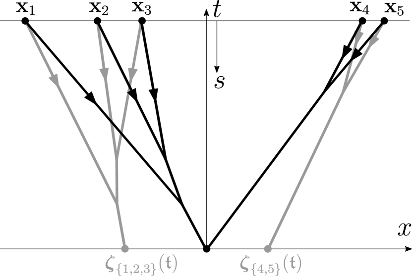
Figure 1. The inertia clusters (gray) and optimal clusters (black). In this figure, $\mathfrak{B}=\{\{1,2,3\},\{4,5\}\}$, and $\mathbf{x}^{{\scriptscriptstyle\prime}}=0$.

Figure 2. Intermediate-time configuration. In this figure, $\mathfrak{C}(1)=\{1\}$, $\mathfrak{C}(2)=\{2\}$, $\mathfrak{C}(3)=\{3\}$, $\mathfrak{C}(4)=\{4,5\}$.

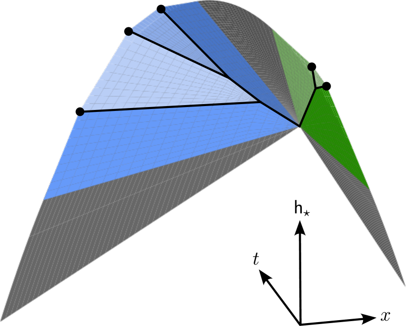
Figure 3. The limit shape. In the gray regions $\mathsf{h}_{\mathrm{\star}}=\mathsf{p}$; in the colored regions $\mathsf{h}_{\mathrm{\star}}$ is piecewise linear.

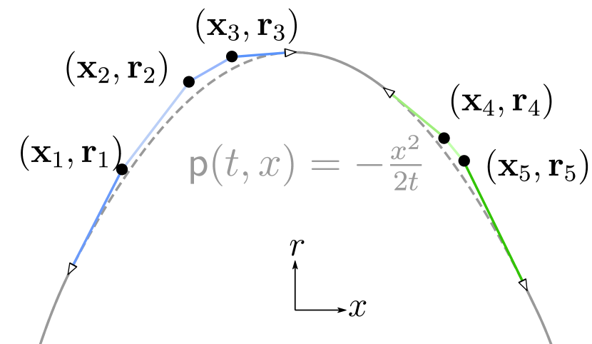
Figure 4. $\mathsf{f}_{\star}=\mathsf{f}_{\star,t,\vec{\mathbf{x}},\vec{\mathbf{r}}}$

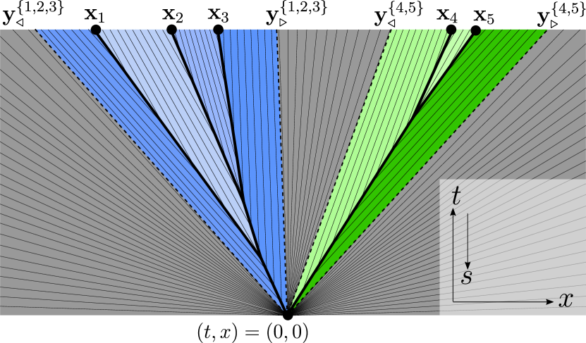
Figure 5. The shocks (thick solid lines) and characteristics (thin solid lines)

2.4. Result: Connection to $I_{\scriptscriptstyle\mathrm{KPZ}}$ and the limit shape

Here, we describe the $n$-point upper-tail rate function $I_{\scriptscriptstyle\mathrm{KPZ}}$ of the KPZ equation and the corresponding limit shape, and show how the moment Lyapunov exponent and the optimal deviation are related to them.

To describe the rate function, fix $t\in(0,\mathfrak{t}\hskip 1.0pt]$, $\mathbf{x}_{1}<\ldots<\mathbf{x}_{n}$. Let $\mathsf{p}(t)=\mathsf{p}(t,x):=-x^{2}/(2t)$. For $\mathbf{r}_{\mathfrak{c}}\geq-\mathsf{p}(t,\mathbf{x}_{\mathfrak{c}})$, $\mathfrak{c}=1,\ldots,n$, let $\mathsf{f}_{\star,t,\vec{\mathbf{x}},\vec{\mathbf{r}}}=\mathsf{f}_{\star}$ be the piecewise $\mathscr{C}^{1}$ function on $\mathbb{R}$ characterized by the properties: $\mathsf{f}_{\star}(\mathbf{x}_{\mathfrak{c}})=\mathbf{r}_{\mathfrak{c}}$, for all $\mathfrak{c}$; $\mathsf{f}_{\star}\geq\mathsf{p}(t)$; $\mathsf{f}_{\star}(x)=\mathsf{p}(t,x)$ for all $|x|$ large enough; $\partial_{x}\mathsf{f}_{\star}$ is constant on $\{\mathsf{f}_{\star}>\mathsf{p}(t)\}\setminus\{\mathbf{x}_{1},\ldots,\mathbf{x}_{n}\}$; $\mathsf{f}_{\star}$ is $\mathscr{C}^{1}$ except at $\mathbf{x}_{1},\ldots,\mathbf{x}_{n}$. See Figure 5. The rate function is

$$I_{\scriptscriptstyle\mathrm{KPZ}}(t,\vec{\mathbf{x}},\vec{\mathbf{r}}):=\int_{\mathbb{R}}\mathrm{d}x\,\big{(}\tfrac{1}{2}(\partial_{x}\mathsf{f}_{\star,t,\vec{\mathbf{x}},\vec{\mathbf{r}}})^{2}-\tfrac{1}{2}(\partial_{x}\mathsf{p}(t))^{2}\big{)}.$$ (2.19)

This rate function coincides with that of a BM that evolves in $x$ conditioned to stay above the parabola $\mathsf{p}(t,x)=-x^{2}/(2t)$. Such a coincidence can be understood from the perspective of Gibbs line ensembles [CH14, CH16], though we arrive at (2.19) through taking the Legendre transform of the moment Lyapunov exponents. This rate function should describe all upper-tail deviations in

$$\mathscr{R}(t,\vec{\mathbf{x}}):=\{\vec{\mathbf{r}}=(\mathbf{r}_{\mathfrak{c}})_{\mathfrak{c}=1}^{n}:\mathbf{r}_{\mathfrak{c}}\geq\mathsf{p}(t,\mathbf{x}_{\mathfrak{c}})\},$$ (2.20)

while positive moments give access the subspace of deviations

$$\mathscr{R}_{\mathrm{conc}}(t,\vec{\mathbf{x}}):=\{\vec{\mathbf{r}}\in\mathscr{R}(t,\vec{\mathbf{x}}):\mathsf{f}_{\star,t,\vec{\mathbf{x}},\vec{\mathbf{r}}}\text{ is concave}\}.$$ (2.21)

Next, let us describe the limit shape $\mathsf{h}_{\mathrm{\star}}=\mathsf{h}_{\mathrm{\star}}(t,x)$. The shape at $t=\mathfrak{t}$ is just $\mathsf{h}_{\mathrm{\star}}(\mathfrak{t}):=\mathsf{f}_{\star}$. For $t<\mathfrak{t}$, the shape is obtained by solving $\partial_{t}\mathsf{h}_{\mathrm{\star}}=\frac{1}{2}(\partial_{x}\mathsf{h}_{\mathrm{\star}})^{2}$ backward in $t$ from $\mathsf{h}(\mathfrak{t})=\mathsf{f}_{\star}$. More precisely, the shape is the entropy solution of the backward equation, which will be described in more detail in Section 8.3. As will be seen there, despite being the entropy solution of the backward equation, $\mathsf{h}_{\mathrm{\star}}$ is a non-entropy solution of the forward equation. In particular, when viewed in forward time, the shocks of $\mathsf{h}_{\mathrm{\star}}$ are non-entropy; see Figure 5 for an illustration.

The result below connects the moment Lyapunov exponent and optimal deviation of the attractive BPs to the rate function and limit shape of the KPZ equation.

Notation for Theorem 2.5.

2. Fix $t$ and $\vec{\mathbf{x}}$; view $I_{\scriptscriptstyle\mathrm{KPZ}}(t,\vec{\mathbf{x}},\vec{\mathbf{r}})=:I_{\scriptscriptstyle\mathrm{KPZ}}(\vec{\mathbf{r}})$ and $L_{\scriptscriptstyle\mathrm{SHE}}(0\xrightarrow{t}(\vec{\mathbf{x}},\vec{\mathfrak{m}}))=:L_{\scriptscriptstyle\mathrm{SHE}}(\vec{\mathfrak{m}})$ as functions on $\mathscr{R}_{\mathrm{conc}}(t,\vec{\mathbf{x}})$ and on $[0,\infty)^{n}$, respectively.

3. Fix any $(\mathbf{x}_{1}<\ldots<\mathbf{x}_{n})$, consider the terminal time $\mathfrak{t}$, take any pair $(\vec{\mathbf{r}},\vec{\mathfrak{m}})\in\mathscr{R}_{\mathrm{conc}}(\mathfrak{t},\vec{\mathbf{x}})^{\circ}\times(0,\infty)^{n}$ that satisfies $(\nabla_{\vec{\mathbf{r}}}I_{\scriptscriptstyle\mathrm{KPZ}})(t,\vec{\mathbf{x}},\vec{\mathbf{r}})=\vec{\mathfrak{m}}$, and let $\mathsf{h}_{\mathrm{\star}}$ and $\boldsymbol{\xi}$ be the corresponding limit shape and optimal deviation, respectively.

4. Let $\vec{\mathbf{x}}$, $\vec{\mathbf{r}}$, and $\vec{\mathfrak{m}}$ be as in Part (b) and take any intermediate time $\mathfrak{t}^{{\scriptscriptstyle\prime}}\in(0,\mathfrak{t}\hskip 1.0pt]$. Traveling in backward time, some of the optimal clusters may have merged by time $s=\mathfrak{t}-\mathfrak{t}^{{\scriptscriptstyle\prime}}$. Let $\{\boldsymbol{\xi}_{\mathfrak{c}}(\mathfrak{t}-\mathfrak{t}^{{\scriptscriptstyle\prime}})\}_{\mathfrak{c}=1}^{n}=\{\mathbf{x}^{{\scriptscriptstyle\prime}}_{1}<\ldots<\mathbf{x}^{{\scriptscriptstyle\prime}}_{n^{\prime}}\}$ denote the distinct positions of the clusters at that time. Accordingly, let $\vec{\mathbf{r}}{}^{\hskip 1.0pt{\scriptscriptstyle\prime}}:=(\mathsf{h}_{\mathrm{\star}}(\mathfrak{t}^{{\scriptscriptstyle\prime}},\mathbf{x}^{{\scriptscriptstyle\prime}}_{\mathfrak{a}}))_{\mathfrak{a}=1}^{n^{\prime}}$, $\mathfrak{C}(\mathfrak{a}):=\{\mathfrak{c}:\boldsymbol{\xi}_{\mathfrak{c}}(\mathfrak{t}-\mathfrak{t}^{{\scriptscriptstyle\prime}})=\mathbf{x}^{{\scriptscriptstyle\prime}}_{\mathfrak{a}}\}$, $\mathfrak{m}^{\hskip 1.0pt{\scriptscriptstyle\prime}}_{\mathfrak{a}}:=\sum_{\mathfrak{c}\in\mathfrak{C}(\mathfrak{a})}\mathfrak{m}_{\mathfrak{c}}$, and $\vec{\mathfrak{m}}{}^{{\scriptscriptstyle\prime}}:=(\mathfrak{m}^{\hskip 1.0pt{\scriptscriptstyle\prime}}_{\mathfrak{a}})_{\mathfrak{a}=1}^{n^{\prime}}$; see Figure 2 for an illustration.

Theorem 2.5.

Notation as above.

1. The functions $I_{\scriptscriptstyle\mathrm{KPZ}}$ and $L_{\scriptscriptstyle\mathrm{SHE}}$ are continuous, strictly convex, and the Legendre transform of each other. Further, $\nabla I_{\scriptscriptstyle\mathrm{KPZ}}=\nabla_{\vec{\mathbf{r}}}I_{\scriptscriptstyle\mathrm{KPZ}}:\mathscr{R}_{\mathrm{conc}}(t,\vec{\mathbf{x}})\to[0,\infty)^{n}$ is a homeomorphism.

2. The trajectories of the shocks in $\mathsf{h}_{\mathrm{\star}}$ and the trajectories of the optimal clusters in $\boldsymbol{\xi}$ coincide.

3. We have

   $$(\nabla_{\vec{\mathbf{r}}}I_{\scriptscriptstyle\mathrm{KPZ}})(\mathfrak{t}^{{\scriptscriptstyle\prime}},\vec{\mathbf{x}}{}^{\hskip 1.0pt{\scriptscriptstyle\prime}},\vec{\mathbf{r}}{}^{\hskip 1.0pt{\scriptscriptstyle\prime}}) =\vec{\mathfrak{m}}{}^{{\scriptscriptstyle\prime}},$$ (2.22)

   $$L_{\scriptscriptstyle\mathrm{SHE}}\big{(}0\xrightarrow{\mathfrak{t}}(\vec{\mathbf{x}},\vec{\mathfrak{m}})\big{)} =L_{\scriptscriptstyle\mathrm{SHE}}\big{(}0\xrightarrow{\mathfrak{t}^{{\scriptscriptstyle\prime}}}(\vec{\mathbf{x}}{}^{\hskip 1.0pt{\scriptscriptstyle\prime}},\vec{\mathfrak{m}}{}^{{\scriptscriptstyle\prime}})\big{)}+\sum_{\mathfrak{a}=1}^{n^{\prime}}L_{\scriptscriptstyle\mathrm{SHE}}\big{(}\mathbf{x}^{{\scriptscriptstyle\prime}}_{\mathfrak{a}}\xrightarrow{\mathfrak{t}-\mathfrak{t}^{{\scriptscriptstyle\prime}}}(\mathbf{x}_{\mathfrak{c}},\mathfrak{m}_{\mathfrak{c}})_{\mathfrak{c}\in\mathfrak{C}(\mathfrak{a})}\big{)}.$$ (2.23)

3. Notation, definitions, tools

3.1. Reduction to $\mathfrak{m}=1$

We begin by explaining how Theorem 2.2, Theorem 2.3, and Corollary 2.4 follow from the special case of $\mathfrak{m}=1$. The key lies in certain scaling relations. Consider the scaling operator $\langle\mathfrak{S}_{\mathfrak{m}}\lambda,\mathsf{f}\rangle:=\langle\mu,\mathsf{f}({\raisebox{-2.15277pt}{\scalebox{1.8}{$\cdot$}}}/\mathfrak{m})\rangle$. The map $\frac{1}{\mathfrak{m}}\mathfrak{S}_{\mathfrak{m}}:\mathfrak{m}\mathscr{P}(\mathbb{R})\to\mathscr{P}(\mathbb{R})$ is a homeomorphism. Applying $\frac{1}{\mathfrak{m}}\mathfrak{S}_{\mathfrak{m}}$ to $\boldsymbol{\mu}_{N}(s)$ gives $\frac{1}{\mathfrak{m}}\mathfrak{S}_{\mathfrak{m}}\boldsymbol{\mu}_{N}(s)=\frac{1}{N\mathfrak{m}}\sum_{i=1}^{N\mathfrak{m}}\delta_{X_{i}(Ts)/(N\mathfrak{m}T)}$. This can be viewed as a unit-mass empirical measure with $N^{\prime}:=N\mathfrak{m}$ being the scaling parameter. We will verify in Appendix A the scaling identities

$$\mathcal{I}\big{(}\tfrac{1}{\mathfrak{m}}\mathfrak{S}_{\mathfrak{m}}\mu)=\tfrac{1}{\mathfrak{m}^{3}}\mathcal{I}(\mu), \mathbb{I}\big{(}\tfrac{1}{\mathfrak{m}}\mathfrak{S}_{\mathfrak{m}}\mu)=\tfrac{1}{\mathfrak{m}^{3}}\mathbb{I}(\mu), \text{for all }\mu\in\mathscr{C}([0,\mathfrak{t}\hskip 1.0pt],\mathfrak{m}\mathscr{P}(\mathbb{R})).$$ (3.1)

The $1/\mathfrak{m}^{3}$ factor absorbs the change in the LDP speed by going from $N$ to $N^{\prime}=N\mathfrak{m}$. Combining what said above shows that Theorem 2.2, Theorem 2.3, and Corollary 2.4 follow from the special case of $\mathfrak{m}=1$.

3.2. The spaces $\mathscr{P}(\mathbb{R})$ and $\mathscr{C}([0,\mathfrak{t}\hskip 1.0pt],\mathscr{P}(\mathbb{R}))$

By Section 3.1, we consider $\mathfrak{m}=1$ only.

Let us introduce some metrics on $\mathscr{P}(\mathbb{R})$ and $\mathscr{C}([0,\mathfrak{t}\hskip 1.0pt],\mathscr{P}(\mathbb{R}))$. Recall the $1$-Wasserstein metric

$$\mathcal{W}(\lambda,\lambda^{\prime}):=\inf\big{\{}\langle\pi,|x-x^{\prime}|\rangle:\pi\in\mathscr{P}(\mathbb{R}^{2}),\,\langle\pi,{\raisebox{-2.15277pt}{\scalebox{1.8}{$\cdot$}}}\otimes 1\rangle=\lambda,\,\langle\pi,1\otimes{\raisebox{-2.15277pt}{\scalebox{1.8}{$\cdot$}}}\rangle=\lambda^{\prime}\big{\}}.$$ (3.2)

The 1-Wasserstein metric on $\mathscr{P}(\mathbb{R})$ permits the inverse-CDF formula:

$$\mathcal{W}(\lambda,\lambda^{\prime}) =\int_{\mathbb{R}}\mathrm{d}x\,\big{|}F[\lambda](x)-F[\lambda^{\prime}](x)\big{|}=\int_{0}^{1}\mathrm{d}a\,\big{|}\mathfrak{X}[\lambda](a)-\mathfrak{X}[\lambda^{\prime}](a)\big{|}.$$ (3.3)

With $\mathbb{R}$ being non-compact, the 1-Wasserstein metric produces a topology stronger than the weak* topology on $\mathscr{P}(\mathbb{R})$. To metrize the weak* topology, we introduce

$$\mathrm{dist}(\lambda,\lambda^{\prime}):=\sum_{k=1}^{\infty}2^{-k}\min\Big{\{}1,\,\int_{-k}^{k}\mathrm{d}x\,\big{|}F[\lambda](x)-F[\lambda^{\prime}](x)\big{|}\Big{\}}.$$ (3.4)

It is not hard to check that $\mathrm{dist}$ metrizes the weak* topology on $\mathscr{P}(\mathbb{R})$. Accordingly,

$$\mathrm{dist}_{[0,\mathfrak{t}\hskip 1.0pt]}(\mu,\mu^{\prime}):=\sup\big{\{}\mathrm{dist}(\mu(s),\mu^{\prime}(s)):s\in[0,\mathfrak{t}\hskip 1.0pt]\big{\}}$$ (3.5)

metrizes the topology on $\mathscr{C}([0,\mathfrak{t}\hskip 1.0pt],\mathscr{P}(\mathbb{R}))$ introduced in Section 2.2. Let us note two useful inequalities related to these metrics. First, by (3.3)–(3.4), $\mathrm{dist}(\lambda,\lambda^{\prime})\leq\mathcal{W}(\lambda,\lambda^{\prime}).$ Next, for any $v_{1},v_{2},\ldots\in(0,1]$ that add to $1$ and any $y_{1},y_{2},\ldots,y^{\prime}_{1},y^{\prime}_{2},\ldots\in\mathbb{R}$,

$$\mathrm{dist}\Big{(}\sum\nolimits_{i}v_{i}\delta_{y_{i}},\sum\nolimits_{i}v_{i}\delta_{y^{\prime}_{i}}\Big{)}\leq\mathcal{W}\Big{(}\sum\nolimits_{i}v_{i}\delta_{y_{i}},\sum\nolimits_{i}v_{i}\delta_{y^{\prime}_{i}}\Big{)}\leq\sum\nolimits_{i}v_{i}\big{|}y_{i}-y^{\prime}_{i}\big{|},$$ (3.6)

which holds thanks to the coupling $\pi(\{y_{i},y^{\prime}_{i}\})=v_{i}$, $i=1,2,\ldots$.

We will need a criterion for a set $S\subset\mathscr{C}([0,\mathfrak{t}\hskip 1.0pt],\mathscr{P}(\mathbb{R}))$ to be precompact. First, by a generalized version of the Arzelá–Ascoli theorem, the set $S$ is precompact if it is equi-continuous and if $\{\mu(s):\mu\in S,s\in[0,\mathfrak{t}\hskip 1.0pt]\}$ is precompact in $\mathscr{P}(\mathbb{R})$; see [Mun00, Thm. 47.1] for example. By the Banach–Alaoglu theorem, for any $b<\infty$, the set $\{\lambda\in\mathscr{P}(\mathbb{R}):\mathrm{supp}(\lambda)\subset[-b,b]\}$ is compact. From this property, it is not hard to show that, for any $b_{1},b_{2},\ldots\to\infty$, the set $\cap_{k=1}^{\infty}\{\lambda\in\mathscr{P}(\mathbb{R}):\lambda(\mathbb{R}\setminus[-b_{k},b_{k}])\leq 1/k\}$ is precompact in $\mathscr{P}(\mathbb{R})$. These properties give the following criterion.

Lemma 3.1.

A set $S\subset\mathscr{C}([0,\mathfrak{t}\hskip 1.0pt],\mathscr{P}(\mathbb{R}))$ is precompact if

1. the set $S$ is equicontinuous with respect to $\mathrm{dist}$, and

2. there exists $b_{k}\to\infty$ such that $\langle\mu(s),\mathbf{1}_{\mathbb{R}\setminus[-b_{k},b_{k}]}\rangle\leq 1/k$, for all $k\in\mathbb{Z}_{>0}$, $\mu\in S$, and $s\in[0,\mathfrak{t}\hskip 1.0pt]$.

Here is a list of useful properties.

Lemma 3.2.

2. For any $\lambda\in\mathscr{P}(\mathbb{R})$ and $\mathsf{f}\in\mathcal{L}^{1}(\mathbb{R},\lambda)$, $\langle\lambda,\mathsf{f}\rangle=\int_{0}^{1}\mathrm{d}a\,\mathsf{f}(\mathfrak{X}[\lambda](a)).$

3. For any $\mu\in\mathscr{C}([0,\mathfrak{t}\hskip 1.0pt],\mathscr{P}(\mathbb{R}))$, the tail mass $\sup_{s\in[0,\mathfrak{t}\hskip 1.0pt]}\langle\mu(s),\mathbf{1}_{\mathbb{R}\setminus[-b,b]}\rangle$ tends to zero as $b\to\infty$.

4. For any $\mu\in\mathscr{C}([0,\mathfrak{t}\hskip 1.0pt],\mathscr{P}(\mathbb{R}))$, for Lebesgue almost every $a\in[0,1]$, $\mathfrak{X}[\mu({\raisebox{-2.15277pt}{\scalebox{1.8}{$\cdot$}}})](a)\in\mathscr{C}[0,\mathfrak{t}\hskip 1.0pt]$.

Part (a) is the standard inverse-CDF formula; Parts (b)–(c) are proven in Appendix A.

3.3. Expressing $\Phi[\lambda]$ in the quantile coordinate

For any $\lambda\in\mathscr{P}(\mathbb{R})$ and $a\in[0,1]$, let

$$a_{-}=a_{-}[\lambda](a) :=\inf\{a^{\prime}\in[0,1]:\mathfrak{X}[\lambda](a^{\prime})=\mathfrak{X}[\lambda](a)\},$$ (3.7a)

$$a_{+}=a_{+}[\lambda](a) :=\sup\{a^{\prime}\in[0,1]:\mathfrak{X}[\lambda](a^{\prime})=\mathfrak{X}[\lambda](a)\}.$$ (3.7b)

Note that $a_{-}<a_{+}$ if and only if $\lambda$ has an atom at $\mathfrak{X}[\lambda](a)$. Refer to the second expression of $\Phi[\lambda]$ in (2.7) and note that $\lambda((-\infty,\mathfrak{X}[\lambda](a)))=a_{-}$ and $\lambda((\mathfrak{X}[\lambda](a),\infty))=(1-a_{+})$. We have

$$\Phi[\lambda]\big{(}\mathfrak{X}[\lambda](a)\big{)}=\begin{cases}\frac{1}{2}-a,&\text{ when }a_{-}=a_{+},\\ \frac{1}{2}-\frac{a_{-}+a_{+}}{2}=\frac{1}{a_{+}-a_{-}}\int_{a_{-}}^{a_{+}}\mathrm{d}a\,(\frac{1}{2}-a),&\text{ when }a_{-}<a_{+}.\end{cases}$$ (3.8)

Since $\mathfrak{X}[\lambda]|_{(a_{-},a_{+})}$ is constant, the expression (3.8) gives, for any $\mathsf{f}\in\mathcal{L}^{1}(\mathbb{R},\lambda)$,

$$\int_{0}^{1}\mathrm{d}a\,\mathsf{f}\big{(}\mathfrak{X}[\lambda](a)\big{)}\cdot\Phi[\lambda]\big{(}\mathfrak{X}[\lambda](a)\big{)}=\int_{0}^{1}\mathrm{d}a\,\mathsf{f}\big{(}\mathfrak{X}[\lambda](a)\big{)}\,(\tfrac{1}{2}-a).$$ (3.9)

3.4. Dividing a measure

Let us introduce a procedure of dividing a given $\mu\in\mathscr{C}([0,\mathfrak{t}\hskip 1.0pt],\mathscr{P}(\mathbb{R}))$ into pieces with constant masses. Fix any $\mathfrak{m}_{1},\ldots,\mathfrak{m}_{n}\in(0,1]$ that add up to $\mathfrak{m}=1$. For any $s\in[0,\mathfrak{t}\hskip 1.0pt]$ and $\mathfrak{c}\in\{1,\ldots,n\}$, consider $F_{\mathfrak{c}}(s,x):=\max\{\min\{F[\mu(s)](x)-(\mathfrak{m}_{1}+\ldots+\mathfrak{m}_{\mathfrak{c}-1}),\mathfrak{m}_{\mathfrak{c}}\},0\}$. Namely, we consider the graph of $F[\mu(s)]({\raisebox{-2.15277pt}{\scalebox{1.8}{$\cdot$}}})$ between the horizontal levels $(\mathfrak{m}_{1}+\ldots+\mathfrak{m}_{\mathfrak{c}-1})$ and $(\mathfrak{m}_{1}+\ldots+\mathfrak{m}_{\mathfrak{c}})$ and shift the graph down so that the lower level is at $0$. The result $F_{\mathfrak{c}}(s,x)$ is the CDF of a measure with total mass $\mathfrak{m}_{\mathfrak{c}}$, and we let $\mu_{\mathfrak{c}}(s)\in\mathfrak{m}_{\mathfrak{c}}\mathscr{P}(\mathbb{R})$ denote that measure.

Here are a few properties of $\mu_{\mathfrak{c}}$. First, $\mu_{\mathfrak{c}}(s)$ is continuous in $s$. To see why, note that, by construction, $|F_{\mathfrak{c}}(s^{\prime},x)-F_{\mathfrak{c}}(s,x)|\leq|F(s^{\prime},x)-F(s,x)|$. Using this property in conjunction with (3.4) and the continuity of $\mu$ gives the continuity of $\mu_{\mathfrak{c}}$. Next, by construction, the measure $\mu_{\mathfrak{c}}(s)$ is supported in $[\mathfrak{X}[\mu(s)](\mathfrak{m}_{1}+\ldots+\mathfrak{m}_{\mathfrak{c}-1}),\mathfrak{X}[\mu_{s}](\mathfrak{m}_{1}+\ldots+\mathfrak{m}_{\mathfrak{c}})]$. Finally, note that $\mu_{\mathfrak{c}}(s)$ and $\mu_{\mathfrak{c}+1}(s)$ can both have an atom at $\mathfrak{X}[\mu(s)](\mathfrak{m}_{1}+\ldots+\mathfrak{m}_{\mathfrak{c}})$.

4. LDP for the attractive BPs: properties of the rate functions

As explained in Section 3.1, we will only consider $\mathfrak{m}=1$, so all deviations take value in $\mathscr{P}(\mathbb{R})$.

4.1. The quantile representation

Here, we show that $\mathcal{I}=\mathbb{I}$ on $\mathscr{C}([0,\mathfrak{t}\hskip 1.0pt],\mathscr{P}(\mathbb{R}))$. To simplify notation, write $\mathfrak{X}[\mu(s)](a)=\mathfrak{X}(s,a)$, $\Phi[\mu(s)](x)=\Phi(s,x)$, and $F[\mu(s)](x):=F(s,x)$.

Case 1: $\boldsymbol{\partial_{s}\mathfrak{X}[\mu]\in\mathcal{L}^{2}([0,\mathfrak{t}\hskip 1.0pt]\times[0,1])}$. We seek to express the terms in (2.9) in the quantile coordinate. Take any $\mathsf{h}\in{\mathscr{C}_{\mathrm{b}}}^{1,1}([0,\mathfrak{t}\hskip 1.0pt],\mathbb{R})$. Under the assumption of Case 1, $\mathfrak{X}(s,a)$ is differentiable in $s$ Lebesgue almost everywhere (a.e.) on $[0,\mathfrak{t}\hskip 1.0pt]\times[0,1]$, so $\frac{\mathrm{d}~{}}{\mathrm{d}s}\mathsf{h}(s,\mathfrak{X}(s,a))-\partial_{s}\mathsf{h}(s,\mathfrak{X}(s,a))=\partial_{x}\mathsf{h}(s,\mathfrak{X}(s,a))\partial_{s}\mathfrak{X}(s,a)$ Lebesgue a.e. Apply $\int\!\!{}_{[0,\mathfrak{t}\hskip 1.0pt]}\mathrm{d}s\int_{0}^{1}\mathrm{d}a$ to both sides. On the left hand side of the result, use Lemma 3.2(a) in reverse to turn the result into $\langle\mu(s),\mathsf{h}(s)\rangle|_{0}^{\mathfrak{t}\hskip 1.0pt}-\int\!\!{}_{[0,\mathfrak{t}\hskip 1.0pt]}\mathrm{d}s\langle\mu,\partial_{s}\mathsf{h}\rangle$, which gives the first two terms in (2.8). Next, use Lemma 3.2(a) to express the last term in (2.8) and the integral term in (2.9) in the quantile coordinate. Collecting the preceding results gives

$$\mathcal{I}(\mu)=\sup_{\mathsf{h}}\int_{0}^{\mathfrak{t}}\mathrm{d}s\int_{0}^{1}\mathrm{d}a\,\Big{(}(\partial_{x}\mathsf{h})_{\mathfrak{X}}(\partial_{s}\mathfrak{X}-\Phi_{\mathfrak{X}})-\frac{1}{2}\big{(}(\partial_{x}\mathsf{h})_{\mathfrak{X}}\big{)}^{2}\Big{)},$$ (4.1)

where the subscript $(\varphi_{\mathfrak{X}})(s,a):=\varphi(t,\mathfrak{X}(s,a))$ means transformation to the quantile coordinate.

Let us simplify (4.1). Within the integral, write $\partial_{x}\mathsf{h}=\mathsf{g}$ and complete the square to get $-\frac{1}{2}(\mathsf{g}_{\mathfrak{X}}-\partial_{s}\mathfrak{X}+\Phi_{\mathfrak{X}})^{2}+\frac{1}{2}(\partial_{s}\mathfrak{X}-\Phi_{\mathfrak{X}})^{2}$, and recognize the contribution of $\frac{1}{2}(\partial_{s}\mathfrak{X}-\Phi_{\mathfrak{X}})^{2}$ as $\mathbb{I}(\mu)$. The supremum is taken over $\mathsf{h}\in{\mathscr{C}_{\mathrm{b}}}^{1,1}([0,\mathfrak{t}\hskip 1.0pt],\mathbb{R})$. Via an approximation argument, we can replace those $\mathsf{h}$s with the $\mathsf{g}$s with $\int\!\!{}_{[0,\mathfrak{t}\hskip 1.0pt]}\mathrm{d}s\,\langle\mu,\mathsf{g}^{2}\rangle<\infty$. Doing so gives

$$\mathcal{I}(\mu)=\mathbb{I}(\mu)-\inf\Big{\{}\int_{0}^{\mathfrak{t}}\mathrm{d}s\int_{0}^{1}\mathrm{d}a\,\frac{1}{2}\big{(}\mathsf{g}_{\mathfrak{X}}-\partial_{s}\mathfrak{X}+\Phi_{\mathfrak{X}}\big{)}^{2}\,:\,\int_{0}^{\mathfrak{t}}\mathrm{d}s\,\langle\mu,\mathsf{g}^{2}\rangle<\infty\Big{\}}.$$ (4.2)

It remains only to show that the infimum in (4.2) is zero. When the CDF $F(s,x)$ strictly increases in $x$ for all $s$, choosing $\mathsf{g}=(\partial_{s}\mathfrak{X})_{F}-\Phi$ completes the proof. Otherwise, take any partition $\Gamma=\{0=s_{0}<s_{1}<\ldots<s_{|\Gamma|}=\mathfrak{t}\}$ of $[0,\mathfrak{t}\hskip 1.0pt]$, let

$$(\partial_{\Gamma}\varphi)(s):=\sum_{j=1}^{|\Gamma|}\frac{\varphi(s_{j})-\varphi(s_{j-1})}{s_{j}-s_{j-1}}\mathbf{1}_{[s_{j-1},s_{j})}(s)$$ (4.3)

denote the discrete time derivative with respect to $\Gamma$, and take $\mathsf{g}(s,x):=(\partial_{\Gamma}\mathfrak{X}({\raisebox{-2.15277pt}{\scalebox{1.8}{$\cdot$}}},F({\raisebox{-2.15277pt}{\scalebox{1.8}{$\cdot$}}},x))(s)-\Phi(s,x)$. Insert this $\mathsf{g}$ into (4.2). The terms $-\Phi_{\mathfrak{X}}$ and $\Phi_{\mathfrak{X}}$ cancel each other. For the discrete-derivative term, note that $\mathfrak{X}(s_{j},F(s_{j},x))_{\mathfrak{X}}:=\mathfrak{X}(s_{j},F(s_{j},\mathfrak{X}(s_{j},a)))$. It is not hard to check that, for every $s_{j}$, the last expression is equal to $\mathfrak{X}(s_{j},a)$ Lebesgue a.e. on $[0,\mathfrak{t}\hskip 1.0pt]$. The resulting integral hence reads $\int\!\!{}_{[0,\mathfrak{t}\hskip 1.0pt]}\mathrm{d}s\int_{0}^{1}\mathrm{d}a\,\frac{1}{2}(\partial_{\Gamma}\mathfrak{X}-\partial_{s}\mathfrak{X})^{2}$. Under the assumption of Case 1, this integral tends to zero as the mesh of $\Gamma$ tends to zero. This completes the proof for Case 1.

Case 2: $\boldsymbol{\partial_{s}\mathfrak{X}[\mu]\notin\mathcal{L}^{2}([0,\mathfrak{t}\hskip 1.0pt]\times[0,1])}$. In this case, by definition, $\mathbb{I}(\mu):=\infty$. Take any partition $\Gamma=\{0=s_{0}<s_{1}<\ldots<s_{|\Gamma|}=\mathfrak{t}\}$ of $[0,\mathfrak{t}\hskip 1.0pt]$ and let $\partial_{\Gamma}$ be as in (4.3). We will show that

$$\mathcal{I}(\mu)+\frac{\mathfrak{t}}{4}\geq\frac{1}{4}\int_{0}^{\mathfrak{t}}\mathrm{d}s\int_{0}^{1}\mathrm{d}a\,\big{(}\partial_{\Gamma}\mathfrak{X}\big{)}^{2}.$$ (4.4)

By the assumption of Case 2 and Lemma 3.2(c), the right hand side of (4.4) tends to $\infty$ as the mesh of $\Gamma$ tends to zero. Hence proving (4.4) will give the desired result $\mathcal{I}(\mu)=\mathbb{I}(\mu)=\infty$.

The proof will invoke a variant of $\mathcal{I}$. Let us introduce this variant and its properties.

$$\mathcal{I}^{\circ}{}_{[s^{\prime},s^{\prime\prime}]}(\mu):=\sup_{\mathsf{h}\in{\mathscr{C}_{\mathrm{b}}}^{1,1}([s^{\prime},s^{\prime\prime}],\mathbb{R})}\Big{\{}\langle\mu(s),\mathsf{h}(s)\rangle\big{|}_{s^{\prime}}^{s^{\prime\prime}}-\int_{s^{\prime}}^{s^{\prime\prime}}\mathrm{d}s\,\langle\mu,\partial_{s}\mathsf{h}\rangle-\int_{s^{\prime}}^{s^{\prime\prime}}\mathrm{d}s\,\langle\mu,(\partial_{x}\mathsf{h})^{2}\rangle\Big{\}}.$$ (4.5)

The following properties are not difficult to verify, which we do in Appendix A.

1. Additivity in time: $\mathcal{I}^{\circ}{}_{[s_{1},s_{2}]}+\mathcal{I}^{\circ}{}_{[s_{2},s_{3}]}=\mathcal{I}^{\circ}{}_{[s_{1},s_{3}]}$.

2. Monotonicity in time: For all $[s_{2},s_{3}]\subset[s_{1},s_{4}]$, $\mathcal{I}^{\circ}{}_{[s_{2},s_{3}]}\leq\mathcal{I}^{\circ}{}_{[s_{1},s_{4}]}$.

3. Convexity: $\mu\mapsto\mathcal{I}^{\circ}{}_{[s^{\prime},s^{\prime\prime}]}(\mu)$ is convex.

4. Space translation invariance: $\mathcal{I}^{\circ}{}_{[s^{\prime},s^{\prime\prime}]}(\mathsf{T}_{0,y}\mu)=\mathcal{I}^{\circ}{}_{[s^{\prime},s^{\prime\prime}]}(\mu)$, where $\mathsf{T}_{0,y}$ translates $\mu$ in space by $y$, namely $\langle\mathsf{T}_{0,y}\mu(s),\mathsf{f}\rangle:=\langle\mu(s),\mathsf{f}({\raisebox{-2.15277pt}{\scalebox{1.8}{$\cdot$}}}-y)\rangle$ for $\mathsf{f}\in\mathscr{C}_{\mathrm{b}}(\mathbb{R})$.

5. For any time-independent $\lambda\in\mathscr{P}(\mathbb{R})$, $\mathcal{I}^{\circ}{}_{[s^{\prime},s^{\prime\prime}]}(\lambda)=0$.

We begin by bounding $\mathcal{I}(\mu)$ from below. Young’s inequality and the property $|\Phi[\mu]|\leq 1/2$ together give $-\Phi[\mu]\partial_{x}\mathsf{h}\geq-\frac{1}{4}-\frac{1}{2}(\partial_{x}\mathsf{h})^{2}$. Insert this inequality into (2.8)–(2.9), and, within the result, move the term $\int\!\!_{[0,\mathfrak{t}\hskip 1.0pt]}\mathrm{d}s\,\langle\mu,-1/4\rangle=-\mathfrak{t}/4$ to the left hand side. Doing so gives $\mathcal{I}(\mu)+\mathfrak{t}/4\geq\mathcal{I}^{\circ}{}_{[0,\mathfrak{t}\hskip 1.0pt]}(\mu)$. Next, we mollify $\mu$. Define the time-space translation operator by $\langle(\mathsf{T}_{s,y}\nu)(s^{\prime}),\mathsf{f}\rangle:=\langle\nu(s^{\prime}+s),\mathsf{f}({\raisebox{-2.15277pt}{\scalebox{1.8}{$\cdot$}}}-y)\rangle$, take $\varphi_{\delta}(x):=\exp(-x^{2}/(2\delta))/\sqrt{2\pi\delta}$, and use $\varphi_{\delta}$ to mollify $\mu$ to get $\mu_{\delta}:=\int_{\mathbb{R}}\mathrm{d}s\int_{\mathbb{R}}\mathrm{d}y\,\varphi_{\delta}(s)\varphi_{\delta}(y)\mathsf{T}_{s,y}\mu$, with the convention $\mu(s)|_{s<0}:=\mu(0)$ and $\mu(s)|_{s>\mathfrak{t}}:=\mu(\mathfrak{t})$. Using Properties (c) and (d) in order gives $\mathcal{I}^{\circ}{}_{[0,\mathfrak{t}\hskip 1.0pt]}(\mu_{\delta})\leq\int_{\mathbb{R}}\mathrm{d}s\int_{\mathbb{R}}\mathrm{d}y\,\varphi_{\delta}(s)\varphi_{\delta}(y)\mathcal{I}^{\circ}{}_{[0,\mathfrak{t}\hskip 1.0pt]}(\mathsf{T}_{s,y}\mu)=\int_{\mathbb{R}}\mathrm{d}s\,\varphi_{\delta}(s)\mathcal{I}^{\circ}{}_{[0,\mathfrak{t}\hskip 1.0pt]}(\mathsf{T}_{s,0}\mu).$ For $s\geq 0$, using Properties (a), (e), and (b) in order gives $\mathcal{I}^{\circ}{}_{[0,\mathfrak{t}\hskip 1.0pt]}(\mathsf{T}_{s,0}\mu)=\mathcal{I}^{\circ}{}_{[0,s]}(\mu(0))+\mathcal{I}^{\circ}{}_{[s,\mathfrak{t}\hskip 1.0pt]}(\mu)\leq 0+\mathcal{I}^{\circ}_{[0,\mathfrak{t}\hskip 1.0pt]}(\mu),$ and similarly for $s<0$. Hence

$$\mathcal{I}^{\circ}{}_{[0,\mathfrak{t}\hskip 1.0pt]}(\mu_{\delta})\leq\Big{(}\int_{\mathbb{R}}\mathrm{d}s\,\varphi_{\delta}(s)\Big{)}\,\mathcal{I}^{\circ}{}_{[0,\mathfrak{t}\hskip 1.0pt]}(\mu)=\mathcal{I}^{\circ}{}_{[0,\mathfrak{t}\hskip 1.0pt]}(\mu)\leq\mathcal{I}(\mu)+\frac{\mathfrak{t}}{4}.$$ (4.6)

Write $\mathcal{I}^{\circ}_{j}:=\mathcal{I}^{\circ}{}_{[s_{j-1},s_{j}]}$. The last bound and Property (a) give $\mathcal{I}(\mu)+\mathfrak{t}/4\geq\mathcal{I}^{\circ}_{1}(\mu_{\delta})+\ldots+\mathcal{I}^{\circ}_{|\Gamma|}(\mu_{\delta})$.

We next bound $\mathcal{I}^{\circ}_{j}(\mu_{\delta})$ from below. Write $F_{\delta}(s,x):=F[\mu_{\delta}(s)](x)$ and $\mathfrak{X}_{\delta}(s,a):=\mathfrak{X}[\mu_{\delta}(s)](a)$ to simplify notation. By the construction of $\mu_{\delta}$, both functions are $\mathscr{C}^{\infty}$. Further, since the mollifier $\varphi_{\delta}$ is strictly positive everywhere, $F_{\delta}(s,x)$ strictly increases in $x$, whereby $F_{\delta}(s,\mathfrak{X}_{\delta}(s,a))=a$ for all $s$ and $a$. Fix any $v\in\mathscr{C}_{\mathrm{c}}^{\infty}(\mathbb{R})$ and let $\mathsf{h}(s,x):=\int_{-\infty}^{x}\mathrm{d}y\,v(F_{\delta}(s,y))$. For this test function, $\frac{\mathrm{d}~{}}{\mathrm{d}s}\mathsf{h}(s,\mathfrak{X}_{\delta}(s,x))=(\partial_{s}\mathsf{h})_{\mathfrak{X}_{\delta}}+(\partial_{x}\mathsf{h})_{\mathfrak{X}_{\delta}}\partial_{s}\mathfrak{X}_{\delta}$ and $(\partial_{x}\mathsf{h})_{\mathfrak{X}_{\delta}}=(v\circ F_{\delta})_{\mathfrak{X}_{\delta}}$, which is equal to $v$ thanks to the relation $F_{\delta}(s,\mathfrak{X}_{\delta}(s,a))=a$. Hence $\frac{\mathrm{d}~{}}{\mathrm{d}s}\mathsf{h}(s,\mathfrak{X}_{\delta}(s,x))-(\partial_{s}\mathsf{h})_{\mathfrak{X}_{\delta}}-(\partial_{x}\mathsf{h})_{\mathfrak{X}_{\delta}}^{2}=v\,\partial_{s}\mathfrak{X}_{\delta}-v^{2}$. Apply $\int\!\!{}_{[s_{j-1},s_{j}]}\mathrm{d}s\int\!\!{}_{[0,1]}\mathrm{d}a$ to both sides and compare the result with (4.5). Doing so gives $\mathcal{I}^{\circ}_{j}(\mu)\geq\int_{0}^{1}\mathrm{d}a\,(v(a)\mathfrak{X}_{\delta}(s,a)|_{s_{j-1}}^{s_{j}}-v(a)^{2}(s_{j}-s_{j-1})).$ Optimizing over $v\in\mathscr{C}_{\mathrm{c}}^{\infty}(\mathbb{R})$ gives $\mathcal{I}^{\circ}_{j}(\mu)\geq(s_{j}-s_{j-1})\int_{0}^{1}\mathrm{d}a\,\frac{1}{4}(\frac{\mathfrak{X}_{\delta}(s_{j},a)-\mathfrak{X}_{\delta}(s_{j-1},a)}{s_{j}-s_{j-1}})^{2}.$

We are now ready to conclude the desired result. Combining the results in the last two paragraphs gives $\mathcal{I}(\mu)+\frac{\mathfrak{t}\hskip 1.0pt}{4}\geq\frac{1}{4}\int\!\!{}_{[0,\mathfrak{t}\hskip 1.0pt]}\mathrm{d}s\int\!\!{}_{[0,1]}\mathrm{d}a\,(\partial_{\Gamma}\mathfrak{X}_{\delta})^{2}.$ With the aid of Lemma 3.2(c), it is not hard to check that $\mathfrak{X}_{\delta}\to\mathfrak{X}$ Lebesgue a.e. on $[0,\mathfrak{t}\hskip 1.0pt]\times[0,1]$. Sending $\delta\to 0$ in the last inequality with the aid of Fatou’s lemma gives the desired result (4.4).

4.2. The rate function $\mathcal{I}_{\star}$ is a good

Here we prove that $\mathcal{I}_{\star}$ is good. Recall from (2.6) that $\mathcal{I}_{\star}$ consists of $\mathcal{I}$ and a dependence on the initial condition. It suffices to show that $\mathcal{I}=\mathbb{I}$ is a good rate function when restricted to $\{\mu:\mu(0)=\mu_{\mathrm{sc}}\}$. We will show that $\mathcal{I}$ is lower-semicontinuous on $\mathscr{C}([0,\mathfrak{t}\hskip 1.0pt],\mathscr{P}(\mathbb{R}))$ and that $S:=\{\mu:\mathbb{I}(\mu)\leq r,\mu(0)=\mu_{\mathrm{sc}}\}$ is precompact.

Let us show the lower semicontinuity of $\mathcal{I}$. We begin with some reductions. Recall from (2.9) that $\mathcal{I}$ is defined as a supremum. Since the supremum of any set of continuous functions is lower semicontinuous, it suffices to check that, for any $\mathsf{h}\in{\mathscr{C}_{\mathrm{b}}}^{1,1}([0,\mathfrak{t}\hskip 1.0pt],\mathbb{R})$,

$$\mathscr{C}([0,\mathfrak{t}\hskip 1.0pt],\mathscr{P}(\mathbb{R}))\to\mathbb{R},\quad\mu\longmapsto\Lambda(\mu,\mathsf{h})-\int_{0}^{\mathfrak{t}}\mathrm{d}s\,\frac{1}{2}\langle\mu,(\partial_{x}\mathsf{h})^{2}\rangle\quad\text{is continuous.}$$ (4.7)

Every term in (2.8) and (2.9) is readily seen to be continuous except for $\int\!\!{}_{[0,\mathfrak{t}\hskip 1.0pt]}\mathrm{d}s\,\langle\mu,\Phi[\mu](\partial_{x}\mathsf{h})\rangle$. It hence suffices to show that, for any $\mathsf{f}\in\mathscr{C}_{\mathrm{b}}(\mathbb{R})$, the map $\mathscr{P}(\mathbb{R})\to\mathbb{R}$: $\lambda\mapsto\langle\lambda,\Phi[\lambda]\mathsf{f}\rangle$ is continuous. To this end, combine Lemma 3.2(a) and the identify (3.9) to get $\langle\lambda,\Phi[\lambda]\mathsf{f}\rangle=\int_{0}^{1}\mathrm{d}a\,(\tfrac{1}{2}-a)\,\mathsf{f}(\mathfrak{X}(a)).$ Take any sequence $\lambda_{k}\Rightarrow\lambda$. Note that $\lambda_{k}\Rightarrow\lambda$ implies to $\mathfrak{X}[\lambda_{k}]\to\mathfrak{X}[\lambda]$ Lebesgue a.e. on $[0,1]$. This property together with the bounded convergence theorem gives $\langle\lambda_{k},\Phi[\lambda_{k}]\mathsf{f}\rangle=\int_{0}^{1}\mathrm{d}a\,(\tfrac{1}{2}-a)\,\mathsf{f}(\mathfrak{X}[\lambda_{k}](a))\to\int_{0}^{1}\mathrm{d}a\,(\tfrac{1}{2}-a)\,\mathsf{f}(\mathfrak{X}(a))=\langle\lambda,\Phi[\lambda]\mathsf{f}\rangle$.

To prepare for the proof of the precompactness, we derive a time-continuity estimate. Recall from (2.11) that $\mathbb{I}$ is defined as an integral over time. Fix $s^{\prime}<s^{\prime\prime}\in[0,\mathfrak{t}\hskip 1.0pt]$, forgo the integral outside $[s^{\prime},s^{\prime\prime}]$, factor out $(s^{\prime\prime}-s^{\prime})$ from the integral, and apply Jensen’s inequality with respect to $(s^{\prime\prime}-s^{\prime})^{-1}\int\!\!{}_{[s^{\prime},s^{\prime\prime}]}\mathrm{d}s\int\!\!{}_{[0,1]}\mathrm{d}a$. Doing so gives $\mathbb{I}(\mu)\geq(s^{\prime\prime}-s^{\prime})((s^{\prime\prime}-s^{\prime})^{-1}\int_{0}^{1}\mathrm{d}a\,\mathfrak{X}[\mu(s)]|_{s^{\prime}}^{s^{\prime\prime}}-(s^{\prime\prime}-s^{\prime})^{-1}\int\!\!{}_{[s^{\prime},s^{\prime\prime}]}\mathrm{d}s\int\!\!{}_{[0,1]}\mathrm{d}a\,\Phi[\mu])^{2}.$ Call the first and second terms within the last square $b$ and $b^{\prime}$ respectively. Use the inequality $(b-b^{\prime})^{2}\geq\frac{1}{2}b^{2}-2{b^{\prime}}^{2}$ and note that $|b^{\prime}|\leq\|\Phi[\mu]\|_{\infty}\leq 1/2$. After being simplified, the result reads $(s^{\prime\prime}-s^{\prime})\mathbb{I}(\mu)+(s^{\prime\prime}-s^{\prime})^{2}/2\geq\int\!\!{}_{[0,1]}\mathrm{d}a\,(\mathfrak{X}[\mu(s^{\prime\prime})]-\mathfrak{X}[\mu(s^{\prime})])^{2}$. By the Cauchy–Schwarz inequality, the last integral is bounded from below by $\int\mathrm{d}a|\mathfrak{X}[\mu(s^{\prime\prime})]-\mathfrak{X}[\mu(s^{\prime})]|$. We arrive at the time-continuity estimate:

$$\int_{0}^{1}\mathrm{d}a\big{|}\,\mathfrak{X}[\mu(s^{\prime\prime})]-\mathfrak{X}[\mu(s^{\prime})]\,\big{|}\leq(s^{\prime\prime}-s^{\prime})\mathbb{I}(\mu)+\tfrac{1}{2}(s^{\prime\prime}-s^{\prime})^{2}.$$ (4.8)

Based on (4.8), we fix $r\in[0,\infty)$ and $\mu_{\mathrm{sc}}\in\mathscr{P}(\mathbb{R})$ and show the precompactness of $S:=\{\mu:\mathbb{I}(\mu)\leq r,\mu(0)=\mu_{\mathrm{sc}}\}$. We will do so by verifying the conditions in Lemma 3.1. Referring to the definition (3.4) of $\mathrm{dist}$, we see that $\mathrm{dist}(\mu(s^{\prime\prime}),\mu(s^{\prime}))$ is bounded by the left hand side of (4.8). Hence the equicontinuity of $S$, which is required by Lemma 3.1(i), follows. To verify the condition in Lemma 3.1(ii), take any $\mu\in S$ and write $\langle\mu(s),\mathbf{1}_{\mathbb{R}\setminus[-b,b]}\rangle$ as $\int\mathrm{d}a\,\mathbf{1}\{|\mathfrak{X}[\mu(s)]|>b\}$. Bound the last integral by $\int\mathrm{d}a\,\mathbf{1}\{|\mathfrak{X}[\mu(0)]|>b/2\}+\int\mathrm{d}a\,\mathbf{1}\{|\mathfrak{X}[\mu(s)]-\mathfrak{X}[\mu(0)]|>b/2\}$. Recognize the former integral as $\langle\mu(0),\mathbf{1}_{\mathbb{R}\setminus[-b/2,b/2]}\rangle$ and bound the second integral by using Markov’s inequality and (4.8) for $(s^{\prime},s^{\prime\prime})=(0,s)$. Doing so gives the bound $(2/b)(s\mathbb{I}(\mu)+s^{2}/2)$, which is at most $(2r\mathfrak{t}+\mathfrak{t}^{2})/b$. Hence, $\langle\mu(s),\mathbf{1}_{\mathbb{R}\setminus[-b,b]}\rangle\leq\langle\mu_{\mathrm{sc}},\mathbf{1}_{\mathbb{R}\setminus[-b/2,b/2]}\rangle+(2r\mathfrak{t}+\mathfrak{t}^{2})/b$. From this, we see that the condition in Lemma 3.1(ii) is satisfied for a suitable choice of $b_{k}\to\infty$.

5. LDP for the attractive BPs: upper bound

Here we prove the LDP upper bound in Theorem 2.2. We achieve this by first establishing the exponential tightness of $\boldsymbol{\mu}_{N}$ (defined at the beginning of Section 5.1) and then proving the weak LDP upper bound (defined at the beginning of Section 5.2). As was explained in Section 3.1, we consider $\mathfrak{m}=1$ only.

5.1. Exponential tightness

Recall that $\boldsymbol{\mu}_{N}$ being exponentially tight means, for any $\varepsilon>0$, there exists a precompact $S\subset\mathscr{C}([0,\mathfrak{t}\hskip 1.0pt],\mathscr{P}(\mathbb{R}))$ such that $\limsup_{N\to\infty}(N^{3}T)^{-1}\log\mathbb{P}[\boldsymbol{\mu}_{N}\notin S]\leq-1/\varepsilon.$

The first step is to device events to control the BMs $B_{i}$ in (2.3). Consider the events $\mathcal{U}_{N}([s_{1},s_{2}],v):=\{\sum_{i=1}^{N}\sup_{s\in[s_{1},s_{2}]}|B_{i}(Ts)-B(Ts_{1})|\leq N^{2}Tv|s_{2}-s_{1}|^{1/3}\}$ and

$$\mathcal{U}_{N}(v) :=\bigcap_{\ell\geq 1}\bigcap_{j=1}^{\ell}\mathcal{U}_{N}\big{(}\big{[}\tfrac{j-1}{\ell}\mathfrak{t},\tfrac{j}{\ell}\mathfrak{t}\hskip 1.0pt\big{]},v\big{)}\,\cap\,\mathcal{U}_{N}\big{(}[0,\mathfrak{t}\hskip 1.0pt],v\big{)}.$$ (5.1)

The random variable $\sum_{i}\sup_{s\in[s_{1},s_{2}]}|B_{i}(Ts)-B_{i}(Ts_{1})|$ has the same law as $\sqrt{T(s_{2}-s_{1})}\sum_{i}|B_{i}(1)|$. Bound the moment generating function of it with the aid of the inequality $\exp(|r|)\leq 2\cosh r$. Use Chernoff’s inequality to turn the bound into $\mathbb{P}[\,\mathcal{U}_{N}([s_{1},s_{2}],v)^{\mathrm{c}}]\leq 2^{N}\exp(-N^{3}Tv^{2}|s_{2}-s_{1}|^{-1/3}/2).$ Under (1.4), the factor $2^{N}$ is negligible compared to $\exp(O(N^{3}T))$. Use the previous bound to fix a large enough $v$ such that $\limsup_{N\to\infty}(N^{3}T)^{-1}\log\mathbb{P}[\mathcal{U}_{N}(v)^{\mathrm{c}}]\leq-1/\varepsilon.$ With $v$ having been fixed, write $\mathcal{U}_{N}(v)=\mathcal{U}_{N}$ hereafter.

We next show that, under $\mathcal{U}_{N}$, all samples of $\boldsymbol{\mu}_{N}$ are contained in a fixed precompact set, which will imply the desired exponential tightness. This amounts to verifying the conditions in Lemma 3.1 — for all realizations of $\boldsymbol{\mu}_{N}$ under $\mathcal{U}_{N}$ — with a fixed choice of $b_{1},b_{2},\ldots\to\infty$.

To verify the equicontinuity required by Lemma 3.1(i), take any $s<s^{\prime}\in[0,\mathfrak{t}\hskip 1.0pt]$ and apply (3.6) to get $\mathrm{dist}(\boldsymbol{\mu}_{N}(s),\boldsymbol{\mu}_{N}(s^{\prime}))\leq\mathcal{W}(\boldsymbol{\mu}_{N}(s),\boldsymbol{\mu}_{N}(s^{\prime}))\leq N^{-1}\sum_{i}|X_{i}(Ts)-X_{i}(Ts^{\prime})|/(NT)$. To bound the last sum, integrate (2.3) over $[Ts,Ts^{\prime}]$ and use $|\mathrm{sgn}|\leq 1/2$. Doing so gives $N^{-1}\sum_{i}|X_{i}(Ts)-X_{i}(Ts^{\prime})|/(NT)\leq|s^{\prime}-s|/2+N^{-1}\sum_{i}|B_{i}(Ts^{\prime})-B_{i}(Ts)|/(NT)$. Further bounding the last sum by the conditions imposed by $\mathcal{U}_{N}$ gives

$$\text{under }\mathcal{U}_{N},\ \frac{1}{N}\sum_{i=1}^{N}\frac{1}{NT}|X_{i}(Ts)-X_{i}(Ts^{\prime})|\leq\frac{1}{2}|s^{\prime}-s|+2v|s^{\prime}-s|^{1/3},\ s<s^{\prime}\in[0,\mathfrak{t}\hskip 1.0pt].$$ (5.2)

Under $\mathcal{U}_{N}$, $\mathrm{dist}(\boldsymbol{\mu}_{N}(s),\boldsymbol{\mu}_{N}(s^{\prime}))\leq|s^{\prime}-s|/2+2v|s^{\prime}-s|^{1/3}$, so the desired equicontinuity holds.

To verify the condition in Lemma 3.1(ii), start by writing

$$\langle\boldsymbol{\mu}_{N}(s),\mathbf{1}_{\mathbb{R}\setminus[-2b,2b]}\rangle\leq\frac{1}{N}\sum_{i=1}^{N}\mathbf{1}\{\tfrac{1}{NT}|X_{i}(Ts)-X_{i}(0)|>b\}+\langle\boldsymbol{\mu}_{N}(0),\mathbf{1}_{\mathbb{R}\setminus(-b,b)}\rangle.$$ (5.3)

The $\limsup_{N\to\infty}$ of the last term is bounded by $\langle\mu_{\mathrm{sc}},\mathbf{1}_{\mathbb{R}\setminus(-b,b)}\rangle$, because $\boldsymbol{\mu}_{N}(0)\Rightarrow\mu_{\mathrm{sc}}$ and because $\mathbb{R}\setminus(-b,b)$ is closed. Next, bound the summand in (5.3) by $b^{-1}|X_{i}(Ts)-X_{i}(0)|/(NT)$ and apply (5.2). The result gives that, under $\mathcal{U}_{N}$, the first term on the right side of (5.3) is bounded by $b^{-1}(s\cdot 2^{-1}+2vs^{1/3})\leq b^{-1}(\mathfrak{t}/2+2v\mathfrak{t}^{1/3})$. These bounds together verify the condition in Lemma 3.1(ii) for $b_{k}:=(\mathfrak{t}/2+2v\mathfrak{t}^{1/3})2k$.

5.2. The weak upper bound

We begin by stating the goal. First, given the exponential tightness, it suffices to prove a weak LDP upper bound, namely the LDP upper bound where the closed set is assumed to be compact. Fix any compact $K\subset\mathscr{C}([0,\mathfrak{t}\hskip 1.0pt],\mathscr{P}(\mathbb{R}))$. Recall $\mathcal{I}_{\star}$ from (2.6). If $K\cap\{\mu:\mu(0)=\mu_{\mathrm{sc}}\}=\emptyset$, then $\inf_{K}\mathcal{I}_{\star}=+\infty$ and the desired upper bound follows trivially. We hence assume $K\cap\{\mu:\mu(0)=\mu_{\mathrm{sc}}\}\neq\emptyset$, whereby $\inf_{K}\mathcal{I}_{\star}=\inf_{K}\mathcal{I}$. Further, recall from (2.9) that $\mathcal{I}$ is defined as a supremum over $\mathsf{h}\in{\mathscr{C}_{\mathrm{b}}}^{1,1}([0,\mathfrak{t}\hskip 1.0pt],\mathbb{R})$. Via an approximation argument, the supremum can be replaced by the one over $\mathsf{h}\in{\mathscr{C}_{\mathrm{c}}}^{\infty}([0,\mathfrak{t}\hskip 1.0pt],\mathbb{R})$. Hence our goal is to show

$$\limsup_{N\to\infty}\frac{1}{N^{3}T}\log\mathbb{P}\big{[}\boldsymbol{\mu}_{N}\in K\big{]}\leq-\inf_{\mu\in K}\sup_{\mathsf{h}\in\mathscr{C}_{\mathrm{c}}^{\infty}([0,\mathfrak{t}\hskip 1.0pt],\mathbb{R})}\Big{\{}\Lambda(\mu,\mathsf{h})-\int_{0}^{\mathfrak{t}\hskip 1.0pt}\mathrm{d}s\,\frac{1}{2}\big{\langle}\mu,(\partial_{x}\mathsf{h})^{2}\big{\rangle}\Big{\}}.$$ (5.4)

Let us use the martingale method [KOV89] to prove (5.4). Take any $\mathsf{h}\in{\mathscr{C}_{\mathrm{c}}}^{\infty}([0,\mathfrak{t}\hskip 1.0pt],\mathbb{R})$ and apply Itô’s calculus to $N^{3}T\langle\boldsymbol{\mu}_{N}(s),\mathsf{h}(s)\rangle=N^{2}T\sum_{i}\mathsf{h}(s,X_{i}(Ts)/(NT))$ with the aid of (2.3) to get

$$N^{3}T\langle\boldsymbol{\mu}_{N}(s),\mathsf{h}(s)\rangle\Big{|}_{0}^{s^{\prime}} -N^{3}T\int_{0}^{s^{\prime}}\mathrm{d}s\,\big{\langle}\boldsymbol{\mu}_{N},\partial_{s}\mathsf{h}+\Phi[\boldsymbol{\mu}_{N}](\partial_{x}\mathsf{h})+\tfrac{1}{2N^{2}T}\partial_{xx}\mathsf{h}\big{\rangle}$$ (5.5a)

$$=NT^{1/2}\sum_{i=1}^{N}\int_{0}^{s^{\prime}}\mathrm{d}B_{i}(s)\,(\partial_{x}\mathsf{h})\big{(}s,\tfrac{1}{NT}X_{i}(Ts)\big{)}.$$ (5.5b)

This result implies that the expression in (5.5a), when viewed as a process in $s^{\prime}$, is a martingale with the quadratic variant $N^{3}T\int_{0}^{s^{\prime}}\mathrm{d}s\,\frac{1}{2}\langle\boldsymbol{\mu}_{N},(\partial_{x}\mathsf{h})^{2}\rangle$. Hence $\mathbb{E}[\exp(N^{3}TU_{N}(\boldsymbol{\mu}_{N}))]=1$, where

$$U_{N}(\mu):=\Lambda(\mu,\mathsf{h})-\int_{0}^{\mathfrak{t}}\mathrm{d}s\,\frac{1}{2}\langle\mu,(\partial_{x}\mathsf{h})^{2}\rangle-\frac{1}{2N^{2}T}\int_{0}^{\mathfrak{t}}\mathrm{d}s\,\langle\mu,\partial_{xx}\mathsf{h}\rangle,$$ (5.6)

and $\Lambda$ was defined in (2.8). Given any Borel $A\subset\mathscr{C}([0,\mathfrak{t}\hskip 1.0pt],\mathscr{P}(\mathbb{R}))$, write

$$\mathbb{P}[\boldsymbol{\mu}_{N}\in A]=\mathbb{E}[\mathbf{1}_{A}(\boldsymbol{\mu}_{N})\exp(-N^{3}TU_{N}(\boldsymbol{\mu}_{N}))\exp(N^{3}TU_{N}(\boldsymbol{\mu}_{N}))],$$ (5.7)

bound the first two factors together by $\sup_{\mu\in A}\exp(-N^{3}TU_{N}(\mu))$, use $\mathbb{E}[\exp(N^{3}TU_{N}(\boldsymbol{\mu}_{N}))]=1$ for the remaining factor, and apply $\limsup_{N}(N^{3}T)^{-1}\log({\raisebox{-2.15277pt}{\scalebox{1.8}{$\cdot$}}})$ to both sides of the result. Doing so gives $\limsup_{N\to\infty}(N^{3}T)^{-1}\log\mathbb{P}[\boldsymbol{\mu}_{N}\in A]\leq\lim_{N\to\infty}\sup_{\mu\in A}U_{N}(\mu)=-\inf_{\mu\in A}\{\Lambda(\mu,\mathsf{h})-\int\!\!{}_{[0,\mathfrak{t}\hskip 1.0pt]}\mathrm{d}s\,\frac{1}{2}\langle\mu,(\partial_{x}\mathsf{h})^{2}\rangle\}.$ Since this holds for all $\mathsf{h}\in{\mathscr{C}_{\mathrm{c}}}^{\infty}([0,\mathfrak{t}\hskip 1.0pt],\mathbb{R})$, we further obtain

$$\limsup_{N\to\infty}\frac{1}{N^{3}T}\log\mathbb{P}\big{[}\boldsymbol{\mu}_{N}\in A\big{]}\leq-\sup_{\mathsf{h}\in\mathscr{C}_{\mathrm{c}}^{\infty}([0,\mathfrak{t}\hskip 1.0pt],\mathbb{R})}\inf_{\mu\in A}\Big{\{}\Lambda(\mu,\mathsf{h})-\int_{0}^{\mathfrak{t}}\mathrm{d}s\,\frac{1}{2}\langle\mu,(\partial_{x}\mathsf{h})^{2}\rangle\Big{\}}.$$ (5.8)

We seek to swap the supremum and infimum on the right hand side. To this end, apply Lemmata 3.2–3.3 in Appendix A.2 in [KL98], with $J_{\mathsf{h}}(\mu)=-\Lambda(\mu,\mathsf{h})+\int\!\!{}_{[0,\mathfrak{t}\hskip 1.0pt]}\mathrm{d}s\,\frac{1}{2}\langle\mu,(\partial_{x}\mathsf{h})^{2}\rangle$. This $J_{\mathsf{h}}(\mu)$ is continuous in $\mu$, as shown after (4.7). The result shows that we can swap the supremum and infimum in (5.8) when $A$ is compact, whereby concluding the desired weak upper bound (5.4).

6. LDP for the attractive BPs: lower bound

We begin by setting up the goal of the proof. As mentioned in Section 3.1, we consider $\mathfrak{m}=1$ only. Indeed, proving the LDP lower bound amounts to proving that, for any $\mu\in\mathscr{C}([0,\mathfrak{t}\hskip 1.0pt],\mathscr{P}(\mathbb{R}))$ and $\varepsilon>0$, $-\mathcal{I}_{\star}(\mu)\leq\liminf_{\varepsilon\to 0}\liminf_{N\to\infty}(N^{3}T)^{-1}\log\mathbb{P}[\mathrm{dist}_{[0,\mathfrak{t}\hskip 1.0pt]}(\boldsymbol{\mu}_{N},\mu)<\varepsilon].$ Recall from (2.6) that, when $\mathcal{I}_{\star}(\mu)<\infty$, we have $\mu(0)=\mu_{\mathrm{sc}}$ and $\mathcal{I}_{\star}(\mu)=\mathbb{I}(\mu)$. Our goal is hence as follows.

Proposition 6.1.

For any $\mu\in\mathscr{C}([0,\mathfrak{t}\hskip 1.0pt],\mathscr{P}(\mathbb{R}))$ with $\mu(0)=\mu_{\mathrm{sc}}$ and $\mathbb{I}(\mu)<\infty$,

$$\liminf_{\varepsilon\to 0}\liminf_{N\to\infty}\frac{1}{N^{3}T}\log\mathbb{P}\big{[}\mathrm{dist}_{[0,\mathfrak{t}\hskip 1.0pt]}(\boldsymbol{\mu}_{N},\mu)<\varepsilon\big{]}\geq-\mathbb{I}(\mu).$$ (6.1)

6.1. Proving a preliminary version of Proposition 6.1

Let us introduce some classes of deviations. We call a deviation $\xi\in\mathscr{C}([0,\mathfrak{t}\hskip 1.0pt],\mathscr{P}(\mathbb{R}))$ clustering if it is of the form $\xi(s)=\sum_{\mathfrak{c}=1}^{n}\mathfrak{m}_{\mathfrak{c}}\delta_{\xi_{\mathfrak{c}}(s)}$, for some $\xi_{1}\leq\ldots\leq\xi_{\mathfrak{c}}\in\mathscr{C}[0,\mathfrak{t}\hskip 1.0pt]$ and some $\mathfrak{m}_{1},\ldots,\mathfrak{m}_{n}\in(0,1]$ that add up to $\mathfrak{m}=1$. We call $\xi_{1},\ldots,\xi_{n}$ the clusters or the trajectories of clusters. We call a deviation Piecewise-Linear(PL)-clustering if it is clustering and the trajectories of its clusters are piecewise linear.

As a first step toward proving Proposition 6.1, here we prove a preliminary version of it where $\mu$ is replaced by a PL-clustering deviation $\xi$. For a PL-clustering deviation, we will use a different way (than $\mathrm{dist}_{[0,\mathfrak{t}\hskip 1.0pt]}$) to measure how close the empirical measure is to the deviation. Recall that the attractive BPs are ordered at the start: $X_{1}(0)\leq\ldots\leq X_{N}(0)$. For a given PL-clustering $\xi$, to each $X_{i}$ assign a cluster $\xi_{\mathfrak{c}}$ via the ordering of the indices:

$$\mathfrak{c}_{N,\xi}(i):=\max\{\mathfrak{c}:\mathfrak{m}_{1}+\ldots+\mathfrak{m}_{\mathfrak{c}}\geq i/N\}, \mathfrak{I}_{N,\xi}(\mathfrak{c}):=\mathfrak{c}_{N,\xi}^{-1}(\{\mathfrak{c}\})=\{i:\mathfrak{c}_{N,\xi}(i)=\mathfrak{c}\}.$$ (6.2)

For $\vec{x}\in(\mathscr{C}[0,T\mathfrak{t}\hskip 1.0pt])^{N}$, set $\mathfrak{D}\mathrm{ist}_{N,s}(\vec{x},\xi):=\max\{|x_{i}(Ts)/(NT)-\xi_{\mathfrak{c}_{N,\xi}(i)}(s)|:i=1,\ldots,N\}$ and $\mathfrak{D}\mathrm{ist}_{N,[s,^{\prime},s^{\prime\prime}]}(\vec{x},\xi):=\sup_{s\in[s^{\prime},s^{\prime\prime}]}\mathfrak{D}\mathrm{ist}_{N,s}(\vec{x},\xi).$ We measure how close the system of attractive BPs is to $\xi$ by $\mathfrak{D}\mathrm{ist}_{N,s}(\vec{X},\xi)$, which is a (much) finer measurement than $\mathrm{dist}(\boldsymbol{\mu}_{N}(s),\xi(s))$. By (3.6),

$$\mathrm{dist}(\boldsymbol{\mu}_{N}(s),\xi(s))\leq\mathfrak{D}\mathrm{ist}_{N,s}\big{(}\vec{X},\xi\big{)}.$$ (6.3)

Hereafter, $c=c(v_{1},v_{2},\ldots)$ denotes a constant that depends only on the designated variables $v_{1},v_{2},\ldots$. We seek to prove the following preliminary version of Proposition 6.1.

Proposition 6.2.

Given any PL-clustering $\xi$, there exists a $c=c(\xi)\in[1,\infty)$ such that

$$\liminf_{r\to 0}\liminf_{N\to\infty} \inf_{\mathfrak{D}\mathrm{ist}_{N,0}(\vec{X},\xi)\leq r}\Big{\{}\frac{1}{N^{3}T}\log\mathbb{P}\big{[}\mathfrak{D}\mathrm{ist}_{N,[0,\mathfrak{t}\hskip 1.0pt]}(\vec{X},\xi)\leq cr\,\big{|}\,\vec{X}(0)\big{]}\Big{\}}\geq-\mathbb{I}(\mu).$$ (6.4)

In (6.4) and similarly hereafter, the conditional probability $\mathbb{P}[\ldots|\vec{X}(0)]$ is viewed as a function of $\vec{X}(0)$, and the infimum is taken over those $\vec{X}(0)$s that satisfy $\mathfrak{D}\mathrm{ist}_{N,0}(\vec{X},\xi)\leq r$.

Proof.

We begin by setting up the notation and outlining the proof. Let $0=s_{0}<s_{1}<\ldots<s_{\ell}=\mathfrak{t}$ be the time between which the clusters of $\xi$ are linear. For a small $\delta>0$ to be fixed shortly, we call $[s_{0},s_{1}-\delta]$, $[s_{1}+\delta,s_{2}-\delta]$, …, $[s_{\ell-1}+\delta,s_{\ell}]$ the linear segments, and call $[s_{1}-\delta,s_{1}+\delta]$, $[s_{2}-\delta,s_{2}+\delta]$, …, the transition segments. To fix the value of $\delta$, consider the maximum speed of all clusters $\dot{\xi}_{\mathrm{max}}:=\sup_{[0,\mathfrak{t}],\mathfrak{c}}|\dot{\xi}_{\mathfrak{c}}|$, and note that, by the definition of the $s_{j}$s, within each $(s_{j-1},s_{j})$, the clusters of $\xi$ either never meet or completely coincide. We fix a small enough $\delta$ such that

$$4\delta\dot{\xi}_{\mathrm{max}}\leq 2\cdot 3^{0}\,r,$$ (6.5)

$$\text{either}\quad|\xi_{\mathfrak{c}}-\xi_{\mathfrak{c}^{\prime}}|_{\text{a linear segment}}>2\cdot 3^{2\ell}r\quad\text{or}\quad(\xi_{\mathfrak{c}}-\xi_{\mathfrak{c}^{\prime}})|_{\text{a linear segment}}=0.$$ (6.6)

Within each linear or transition segment $[s^{\prime},s^{\prime\prime}]$, we seek to prove a bound of the form:

$$\liminf_{N\to\infty}\inf_{\mathfrak{D}\mathrm{ist}_{N,s^{\prime}}(\vec{X},\xi)\leq\text{error}}\Big{\{}\frac{1}{N^{3}T}\log\mathbb{P}\big{[}\,\text{controlling event}[s^{\prime},s^{\prime\prime}]\,\big{|}\,\vec{X}(Ts^{\prime})\,\big{]}\Big{\}}\geq-\text{cost}[s^{\prime},s^{\prime\prime}].$$

The precise version of this inequality will be stated in (6.9) and (6.18). The controlling event ensures that $\mathfrak{D}\mathrm{ist}_{N,[s^{\prime},s^{\prime\prime}]}(\vec{X},\xi)$ is small. To facilitate the control, we will choose a suitable error and require $\mathfrak{D}\mathrm{ist}_{N,s^{\prime}}(\vec{X},\xi)\leq\text{error}$. We will construct these events in such a way that, for any consecutive segments, the controlling event of the former implies the required error bound of the latter. This way the results within the segments can be concatenated. Within a linear segment, we will take $\text{cost}[s^{\prime},s^{\prime\prime}]=\mathbb{I}_{[s^{\prime},s^{\prime\prime}]}(\xi)$, which is optimal. Within a transition segment, we will take a cost that, despite being suboptimal, is negligible as $\delta\to 0$.

Let us carry out the analysis within the linear segments and transition segments separately.

Step 1: analysis within a linear segment. Let us set up the notation and state the desired bound precisely. Fix a linear segment $[s^{\prime},s^{\prime\prime}]$ and define the controlling event as

$$\mathcal{C}_{N,\beta}[s^{\prime},s^{\prime\prime}]:=\big{\{}\mathfrak{D}\mathrm{ist}_{N,[s^{\prime},s^{\prime\prime}]}(\vec{X},\xi)<3^{\beta}r\big{\}}.$$ (6.7)

Hereafter, $\beta\in\mathbb{Z}\cap[0,2\ell)$ is an auxiliary parameter. Let $\mathbb{I}_{[s^{\prime},s^{\prime\prime}]}$ be the analog of $\mathbb{I}$ where the time integral (see (2.11)) is restricted to $[s^{\prime},s^{\prime\prime}]$ and let $\dot{\varphi}:=\mathrm{d}\varphi/\mathrm{d}s$. It is readily checked that

$$\text{for a clustering }\nu=\sum\nolimits_{\mathfrak{c}}\mathfrak{m}_{\mathfrak{c}}\delta_{\nu_{\mathfrak{c}}},\qquad\mathbb{I}_{[s^{\prime},s^{\prime\prime}]}(\nu)=\int_{s^{\prime}}^{s^{\prime\prime}}\mathrm{d}s\,\sum\nolimits_{\mathfrak{c}}\frac{\mathfrak{m}_{\mathfrak{c}}}{2}\big{(}\dot{\nu_{\mathfrak{c}}}-\Phi[\nu](\nu_{\mathfrak{c}})\big{)}^{2}.$$ (6.8)

The desired bound within the linear segment $[s^{\prime},s^{\prime\prime}]$ is

$$\liminf_{N\to\infty}\inf_{\mathfrak{D}\mathrm{ist}_{N,s^{\prime}}(\vec{X},\xi)\leq 3^{\beta}r}\Big{\{}\frac{1}{N^{3}T}\log\mathbb{P}\big{[}\,\mathcal{C}_{N,\beta+1}[s^{\prime},s^{\prime\prime}]\,\big{|}\,\vec{X}(Ts^{\prime})\,\big{]}\Big{\}}\geq-\mathbb{I}_{[s^{\prime},s^{\prime\prime}]}(\xi).$$ (6.9)

Recall from (6.6) that, within $[s^{\prime},s^{\prime\prime}]$, any pair of clusters either stay strictly apart or completely coincide. After combining those clusters that completely coincide, we have

$$|\xi_{\mathfrak{c}}-\xi_{\mathfrak{c}^{\prime}}|_{[s^{\prime},s^{\prime\prime}]}>2\cdot 3^{2\ell}r,\qquad\forall\mathfrak{c}\neq\mathfrak{c}^{\prime}.$$ (6.10)

The first step of proving (6.9) is to set up Girsanov’s transform. Within $[s^{\prime},s^{\prime\prime}]$, the cluster $\xi_{\mathfrak{c}}$ travels at a constant velocity $\mathrm{d}\xi_{\mathfrak{c}}/\mathrm{d}s:=\dot{\xi}_{\mathfrak{c}}$. Letting $v_{\mathfrak{c}}:=\dot{\xi}_{\mathfrak{c}}-\phi_{\mathfrak{c}}$, where $\phi_{\mathfrak{c}}:=\tfrac{1}{2}(\ldots-\mathfrak{m}_{\mathfrak{c}-1}+\mathfrak{m}_{\mathfrak{c}+1}+\ldots)$, we seek to apply Girsanov’s transform to turn $\mathbb{P}$ into another law $\mathbb{Q}$ where

$$\text{under }\mathbb{Q},\qquad\mathrm{d}X_{i}=\sum_{j=1}^{N}\frac{1}{2}\mathrm{sgn}(X_{j}-X_{i})\mathrm{d}s+Nv_{\mathfrak{c}_{N,\xi}(i)}\mathrm{d}s+\mathrm{d}B_{i}.$$ (6.11)

In plain words, we pursue a “strategy” where each $X_{i}$ receives an additional drift $Nv_{\mathfrak{c}_{N,\xi}(i)}$. The term $\dot{\xi}_{\mathfrak{c}}$ in $v_{\mathfrak{c}}$ helps $X_{i}(T{\raisebox{-2.15277pt}{\scalebox{1.8}{$\cdot$}}})/(NT)$ follow the cluster $\xi_{\mathfrak{c}}$, while the term $-\phi_{\mathfrak{c}}$ counters the “pulling” from those particles with a different assigned cluster, namely the effect of the drift $\sum_{j\notin\mathfrak{I}_{N,\xi}(\mathfrak{c})}\mathrm{sgn}(X_{j}-X_{i})/2$. Hereafter, we will use the phrase “pulling” similarly, to refer to the effect of the drift coming from a set of particles.

The next step is to set up a stopping time and prepare the relevant properties. Let $\sigma$ be the first time when the condition required by $\mathcal{C}_{N,\beta+1}[s^{\prime},s^{\prime\prime}]$ is violated, namely $\sigma:=\inf\{s\in[s^{\prime},s^{\prime\prime}]:|X_{i}(Ts)/(NT)-\xi_{\mathfrak{c}_{N,\xi}(i)}(s)|=3^{\beta+1}r,\text{for some }i\}$. Since $\beta<2\ell$, by (6.10), particles with different assigned clusters stay strictly ordered within $[s^{\prime},\sigma]$. This property implies, for any $i\in\mathfrak{I}_{N,\xi}(\mathfrak{c})$, the pulling from particles outside $\mathfrak{I}_{N,\xi}(\mathfrak{c})$ is given by $\sum_{j\notin\mathfrak{I}_{N,\xi}(\mathfrak{c})}\frac{1}{2}\mathrm{sgn}(j-i)$. The last expression sums to $N\frac{1}{2}(\ldots-\mathfrak{m}_{\mathfrak{c}-1}+\mathfrak{m}_{\mathfrak{c}+1}+\ldots)=N\phi_{\mathfrak{c}}$. Hence, within $s\in[s^{\prime},\sigma]$ and for each $i\in\mathfrak{I}_{N,\xi}(\mathfrak{c})$,

$$\sum_{j=1}^{N}\frac{1}{2}\mathrm{sgn}\big{(}\tfrac{1}{NT}X_{j}(Ts)-\tfrac{1}{NT}X_{i}(Ts)\big{)}=\sum_{j\in\mathfrak{I}_{N,\xi}(\mathfrak{c})}\frac{1}{2}\mathrm{sgn}\big{(}\tfrac{1}{NT}X_{j}(Ts)-\tfrac{1}{NT}X_{i}(Ts)\big{)}+N\phi_{\mathfrak{c}}.$$ (6.12)

Having set up the stopping time $\sigma$, we next analyze the evolution of the particles within $s\in[s^{\prime},\sigma]$ and under the condition $\mathfrak{D}\mathrm{ist}_{N,s^{\prime}}(\vec{X},\xi)\leq 3^{\beta}r,$ which is required in (6.9). We will analyze separately the evolution of the center of mass (defined later) relative to their assigned clusters and the evolution of a particle relative to its center of mass. Hereafter, unless otherwise noted, $s\in[s^{\prime},\sigma]$.

We now define the center of masses and analyze their evolution. Let $X_{\mathfrak{c}}:=\sum_{i\in\mathfrak{I}_{N,\xi}(\mathfrak{c})}X_{i}/(N\mathfrak{m}_{\mathfrak{c}})$ be the center of mass. Take the average of (6.11) over $i\in\mathfrak{I}_{N,\xi}(\mathfrak{c})$. The pulling from within $i\in\mathfrak{I}_{N,\xi}(\mathfrak{c})$ averages to zero; the pulling from outside of $\mathfrak{I}_{N,\xi}(\mathfrak{c})$ averages to $\phi_{\mathfrak{c}}$ by (6.12). Hence $\mathrm{d}X_{\mathfrak{c}}=N\dot{\xi}_{\mathfrak{c}}\mathrm{d}s+\mathrm{d}B_{\mathfrak{c}}$, where $B_{\mathfrak{c}}:=\sum_{i\in\mathfrak{I}_{N,\xi}(\mathfrak{c})}B_{i}/(N\mathfrak{m}_{\mathfrak{c}})$. Integrating this equation gives $|X_{\mathfrak{c}}(Ts)/(NT)-\xi_{\mathfrak{c}}(s)|\leq|X_{\mathfrak{c}}(Ts^{\prime})/(NT)-\xi_{\mathfrak{c}}(s^{\prime})|+|B_{\mathfrak{c}}(Ts)-B_{\mathfrak{c}}(Ts^{\prime})|/(NT)$. Under the condition $\mathfrak{D}\mathrm{ist}_{N,s^{\prime}}(\vec{X},\xi)\leq 3^{\beta}r,$ the first term on the right hand side is at most $3^{\beta}r$, so $|X_{\mathfrak{c}}(Ts)/(NT)-\xi_{\mathfrak{c}}(s)|\leq 3^{\beta}r+|B_{\mathfrak{c}}(Ts)-B_{\mathfrak{c}}(Ts^{\prime})|/(NT)$.

We next analyze the motion of a particle relative to its center of mass. Fix any $\mathfrak{c}$. As seen in (6.12), a particle with $i\in\mathfrak{I}_{N,\xi}(\mathfrak{c})$ feels the pulling from within and outside of $\mathfrak{I}_{N,\xi}(\mathfrak{c})$. The former should only pull particles in $\mathfrak{I}_{N,\xi}(\mathfrak{c})$ closer together. To make this statement precise, consider the particles without the inner pulling: $\mathrm{d}Y_{i}=N\phi_{\mathfrak{c}}\mathrm{d}s+\mathrm{d}B_{i},$ for $i\in\mathfrak{I}_{N,\xi}(\mathfrak{c})$ and with $Y_{i}(Ts^{\prime})=X_{i}(Ts^{\prime})$. The center of mass of these $Y_{i}$s coincides with $X_{\mathfrak{c}}$, as can be seen by averaging the preceding evolutionary equations of $Y_{i}$. To compare $X_{i}$ and $Y_{i}$ relative to their center of mass, we consider their gap processes and use a comparison result from [Sar19]. Write $\mathfrak{I}_{N,\xi}(\mathfrak{c})=\{i_{1},i_{1}+1,\ldots\}$, rank $\{X_{i}(Ts)\}_{i\in\mathfrak{I}_{N,\xi}}$ to get $X_{(i_{1})}(Ts)\leq X_{(i_{1}+1)}(Ts)\leq\ldots$, and let $Z_{i}(Ts):=X_{(i+1)}(Ts)-X_{(i)}(Ts)$ be the gap process. Do the same for the $Y_{i}$s and call the gap process $\overline{Z}_{i}$. Theorem 3.1 from [Sar19], which is a pathwise comparison result, gives that $Z_{i}\leq\overline{Z}_{i}$ on $[Ts^{\prime},T\sigma]$. This together with the fact that the $X_{i}$s and $Y_{i}$s have the same center of mass gives $\max\{|X_{i}(Ts)-X_{\mathfrak{c}}(Ts)|:i\in\mathfrak{I}_{N,\xi}(\mathfrak{c})\}\leq\max\{|Y_{i}(Ts)-X_{\mathfrak{c}}(Ts)|:i\in\mathfrak{I}_{N,\xi}(\mathfrak{c})\}$. To bound the right hand side, integrate the evolutionary equations of $Y_{i}$ and of $X_{\mathfrak{c}}$ over $[Ts^{\prime},Ts]$ and take the difference of the results to get $|Y_{i}(Ts)-X_{\mathfrak{c}}(Ts)|\leq|X_{i}(Ts^{\prime})-X_{\mathfrak{c}}(Ts^{\prime})|+|(B_{i}-B_{\mathfrak{c}})(Ts)-(B_{i}-B_{\mathfrak{c}})(Ts^{\prime})|$. Under the condition $\mathfrak{D}\mathrm{ist}_{N,s^{\prime}}(\vec{X},\xi)\leq 3^{\beta}r,$ the first term on the right hand side is at most $NT3^{\beta}r$. Hence, for all $i\in\mathfrak{I}_{N,\xi}(\mathfrak{c})$ and within $s\in[s^{\prime},\sigma]$, $|X_{i}(Ts)-X_{\mathfrak{c}}(Ts)|\leq NT3^{\beta}r+\max\{|(B_{i}-B_{\mathfrak{c}})(Ts)-(B_{i}-B_{\mathfrak{c}})(Ts^{\prime})|:i\in\mathfrak{I}_{N,\xi}(\mathfrak{c})\}.$

Based on what we obtained so far, we now complete the proof of (6.9). The results in the last two paragraphs give, under the condition $\mathfrak{D}\mathrm{ist}_{N,s^{\prime}}(\vec{X},\xi)\leq 3^{\beta}r$ and within $s\in[s^{\prime},\sigma]$,

$$\big{|}\tfrac{1}{NT}X_{i}(Ts)-\xi_{\mathfrak{c}_{N,\xi}(i)}(s)\big{|}\leq 2\cdot 3^{\beta}r+\tfrac{3}{NT}\max\big{\{}|B_{i}(Ts)-B_{i}(Ts^{\prime})|:i=1,\ldots,N\big{\}}.$$ (6.13)

Invoke a small parameter $r^{\prime}$ and consider the event $\mathcal{E}_{N}(r^{\prime}):=\{|B_{i}(Ts)-B_{i}(Ts^{\prime})|<NTr^{\prime},\forall s\in[s^{\prime},s^{\prime\prime}],\forall i=1,\ldots,N\}$. Under $\mathcal{E}_{N}(r^{\prime})$ and for $r^{\prime}<3^{\beta}r/3$, the right hand side of (6.13) is strictly less than $3^{\beta+1}r$. Hence, given $\mathfrak{D}\mathrm{ist}_{N,s^{\prime}}(\vec{X},\xi)\leq 3^{\beta}r$, $\mathcal{E}_{N}(r^{\prime})\subset\{\sigma>s^{\prime\prime}\}\subset\mathcal{C}_{N,\beta}[s^{\prime},s^{\prime\prime}]$. Now apply Lemma C.1(a) with the $v_{i}=v_{\mathfrak{c}_{N,\xi}(i)}$ defined above (6.11) and with $\mathcal{E}=\mathcal{E}_{N}(r^{\prime})$. In the result, recognize that $(s^{\prime\prime}-s^{\prime})\sum_{i=1}^{N}v_{\mathfrak{c}_{N,\xi}(i)}^{2}/(2N)=\mathbb{I}_{[s^{\prime},s^{\prime\prime}]}(\xi)$ with the aid of (6.8). Then, bound $\sum_{i=1}^{N}|v_{\mathfrak{c}_{N,\xi}(i)}|r^{\prime}/(NT)\leq c(\xi)r^{\prime},$ and $(N^{3}T)^{-1}\log\mathbb{Q}[\mathcal{E}_{N}(r^{\prime})]\geq-c\exp(-N^{2}Tr^{\prime}{}^{2}/(c\,(s^{\prime\prime}-s^{\prime})))/(N^{2}T).$ Sending $N\to\infty$ first and $r^{\prime}\to 0$ later yields the desired result (6.9).

Step 2: analysis within a transition segment. Let us set up the notation and state the desired bound precisely. Fix a transition segment $[s^{\prime},s^{\prime\prime}]$, consider the line (in the $(s,x)$ plane) that connects $(s^{\prime},\xi_{\mathfrak{c}_{N,\xi}(i)}(s^{\prime}))$ and $(s^{\prime\prime},\xi_{\mathfrak{c}_{N,\xi}(i)}(s^{\prime\prime}))$, and let

$$w_{i}=w_{i}[s^{\prime},s^{\prime\prime}]:=\frac{\xi_{\mathfrak{c}_{N,\xi}(i)}(s^{\prime\prime})-\xi_{\mathfrak{c}_{N,\xi}(i)}(s^{\prime})}{s^{\prime\prime}-s^{\prime}}=\frac{N}{s^{\prime\prime}-s^{\prime}}\int_{(i-1)/N}^{i/N}\mathrm{d}a\,\big{(}\mathfrak{X}[\xi(s^{\prime\prime})]-\mathfrak{X}[\xi(s^{\prime})]\big{)}$$ (6.14)

be the velocity when traveling along the line. Define the controlling event and and the cost as

$$\mathcal{C}^{\prime}_{N,\beta}[s^{\prime},s^{\prime\prime}] :=\Big{\{}\,\Big{|}\tfrac{1}{NT}X_{i}(Ts)-\xi_{\mathfrak{c}_{N,\xi}(i)}(s^{\prime})-(s-s^{\prime})w_{i}\Big{|}\leq 3^{\beta}r,\forall s\in[s^{\prime},s^{\prime\prime}],\forall i\Big{\}},$$ (6.15)

$$\mathrm{Cost}_{[s^{\prime},s^{\prime\prime}]}(\lambda,\lambda^{\prime}) :=\frac{s^{\prime\prime}-s^{\prime}}{2}\Big{(}\int_{0}^{1}\mathrm{d}a\,\Big{(}\frac{|\mathfrak{X}[\lambda^{\prime}]-\mathfrak{X}[\lambda]|}{s^{\prime\prime}-s^{\prime}}+\frac{1}{2}\Big{)}^{2},$$ (6.16)

By (6.5), it is not hard to check from (6.15) that

$$\mathcal{C}^{\prime}_{N,\beta}[s^{\prime},s^{\prime\prime}]\subset\big{\{}\mathfrak{D}\mathrm{ist}_{N,[s^{\prime},s^{\prime\prime}]}\big{(}\vec{X},\xi\big{)}\leq 3^{\beta+1}r\big{\}}.$$ (6.17)

The desired bound within the transition segment is

$$\liminf_{N\to\infty}\ \inf\Big{\{}\frac{1}{N^{3}T}\log\mathbb{P}\big{[}\,\mathcal{C}^{\prime}_{N,\beta+1}[s^{\prime},s^{\prime\prime}]\,\big{|}\, \vec{X}(Ts^{\prime})\big{]}\Big{\}}\geq-\mathrm{Cost}_{[s^{\prime},s^{\prime\prime}]}(\xi(s^{\prime}),\xi(s^{\prime\prime})),$$ (6.18)

where the infimum runs over $\mathfrak{D}\mathrm{ist}_{N,s^{\prime}}(\vec{X},\xi(s^{\prime}))\leq 3^{\beta}r$, just like in Step 1. As said, the cost here is suboptimal. Later when applying (6.18), we will make the segment $[s^{\prime},s^{\prime\prime}]$ short so that the collective cost (over all transition segments) becomes negligible.

To prove (6.18), consider the law $\mathbb{Q}$ under which $\mathrm{d}X_{i}=Nw_{\mathfrak{c}_{N,\xi}(i)}\mathrm{d}s+\mathrm{d}B_{i}.$ Apply Lemma C.1(b) with $v_{i}=w_{\mathfrak{c}_{N,\xi}(i)}$, $J_{i}=\{1,\ldots,N\}$, $\mathcal{E}=\mathcal{C}^{\prime}_{N,\beta}[s^{\prime},s^{\prime\prime}]$, and $p=2$. It is readily checked that $\inf_{\mathfrak{D}\mathrm{ist}_{N,s^{\prime}}(\vec{X},\xi(s^{\prime}))\leq 3^{\beta}r}(N^{3}T)^{-1}\log\mathbb{Q}[\,\mathcal{C}^{\prime}_{N,\beta+1}[s^{\prime},s^{\prime\prime}]\,|\,\vec{X}(Ts^{\prime})\,]$ tends to zero as $N\to\infty$. To bound $(s^{\prime\prime}-s^{\prime})(2N)^{-1}\sum_{i}(w_{i}{}^{2}+1/2)$, add $1/2$ to both sides of (6.14), square both sides, apply the Cauchy–Schwarz inequality over $\int\!\!{}_{[(i-1)/N,i/N]}\mathrm{d}a$, and apply $(s^{\prime\prime}-s^{\prime})(2N)^{-1}\sum_{i}$. Doing so gives $(s^{\prime\prime}-s^{\prime})(2N)^{-1}\sum_{i}(w_{i}{}^{2}+1/2)\leq\mathrm{Cost}_{[s^{\prime},s^{\prime\prime}]}(\xi(s^{\prime}),\xi(s^{\prime\prime})).$ The desired result (6.18) hence follows.

Step 3: Combining Steps 1–2 to complete the proof. Apply (6.9) and (6.18) in alternating order over the segments $[s_{0},s_{1}-\delta]$, $[s_{1}-\delta,s_{1}+\delta]$, …, with $\beta=0,1,\ldots,2\ell-1$. By (6.7) and (6.15), $\mathcal{C}_{N,1}[s_{0},s_{1}-\delta]\subset\{\mathfrak{D}\mathrm{ist}_{N,s_{1}-\delta}(\vec{X},\xi)\leq 2\cdot 3^{1}\}$, $\mathcal{C}^{\prime}_{N,2}[s_{1}-\delta,s_{1}+\delta]\subset\{\mathfrak{D}\mathrm{ist}_{N,s_{1}+\delta}(\vec{X},\xi)\leq 2\cdot 3^{2}\}$, …, so the resulting bounds can be concatenated. Recall that $\delta$ is chosen so that (6.6) holds. With $\xi$ being PL-clustering, we can indeed choose $\delta$ such that $\delta\leq c(\xi)r$. By (6.7) and (6.17), under the controlling events, $|X_{i}(Ts)/(NT)-\xi_{\mathfrak{c}_{N,\xi}(i)(s)}|\leq 3^{2\ell}r$, for all $s\in[0,\mathfrak{t}\hskip 1.0pt]$ and $i=1,\ldots,N$. Finally, the collective cost of achieving the controlling events is $\sum\mathbb{I}_{[s^{\prime},s^{\prime\prime}]}(\xi)+\sum\mathrm{Cost}_{[s^{\prime},s^{\prime\prime}]}(\xi(s^{\prime}),\xi(s^{\prime\prime}))$, where the first sum runs over all linear segments and the second runs over all transition segments. The first sum is at most $\mathbb{I}(\xi)$, while the second sum tends to zero as $\delta$ tends to zero, as is readily checked from (6.16). Recall that $\delta$ is chosen so that (6.5)–(6.6) hold. As $r\to 0$, the so chosen $\delta$ also tends to $0$. This completes the proof of Proposition 6.2. ∎

6.2. Proving Proposition 6.1 under Assumption 6.3

Based on the results in Section 6.1, here we prove Proposition 6.1 under an additional assumption. Identify $\{\lambda\in\mathscr{P}(\mathbb{R}):\mathrm{supp}(\lambda)\subset[-b,b]\}$ with $\mathscr{P}[-b,b]$. Namely, view those measures supported in $[-b,b]$ as measures on $[-b,b]$.

Assumption 6.3.

There exists a $b<\infty$ such that $\{\boldsymbol{\mu}_{N}(0)\}_{N\in\mathbb{Z}_{>0}},\{\mu(s)\}_{s\in[0,\mathfrak{t}\hskip 1.0pt]}\subset\mathscr{P}[-b,b]$.

Namely, we assume that $\boldsymbol{\mu}_{N}(0)$ and $\mu(s)$ have a compact support, uniformly over $N\in\mathbb{Z}_{>0}$ and $s\in[0,\mathfrak{t}\hskip 1.0pt]$. Fixing a $\mu$ and $\boldsymbol{\mu}_{N}(0)$ that satisfy $\mathbb{I}(\mu)<\infty$, $\boldsymbol{\mu}_{N}(0)\Rightarrow\mu(0)$, and Assumption 6.3, we seek to prove (6.1) for this $\mu$ and $\boldsymbol{\mu}_{N}(0)$.

The proof requires an approximation tool. We state it here and put its proof in Appendix B:

$$\inf\big{\{} \mathrm{dist}_{[s^{\prime},s^{\prime\prime}]}(\xi,\mu)+|\mathbb{I}_{[s^{\prime},s^{\prime\prime}]}(\xi)-\mathbb{I}_{[s^{\prime},s^{\prime\prime}]}(\mu)|\,:$$ (6.19a)

$$\xi\text{ is PL-clustering },\mathrm{supp}(\xi(s))\subset[-b,b],\forall s\in[s^{\prime},s^{\prime\prime}]\big{\}}=0.$$ (6.19b)

Let us outline the proof. We will construct a small $s_{0}$ and use (6.19) to construct a PL-clustering $\xi$ that approximates $\mu$, and perform analysis over $[0,s_{0}]$ and $[s_{0},\mathfrak{t}\hskip 1.0pt]$ separately.

Let us construct $s_{0}$ and $\xi$. Fix $\varepsilon>0$. By the assumption $\mathbb{I}(\mu)<\infty$, $\partial_{s}\mathfrak{X}[\mu]\in\mathcal{L}^{2}([0,\mathfrak{t}\hskip 1.0pt]\times[0,1])$. Using this property and the time continuity of $\mu$ to find an $s_{0}$ such that $\mathrm{Cost}_{[0,s_{0}]}(\mu(0),\mu(s_{0}))<\varepsilon$ and $\sup_{[0,s_{0}]}\mathrm{dist}(\mu(s),\mu(s_{0}))<\varepsilon$. Turning to the construction of $\xi$, we begin by noting that $\mathrm{Cost}_{[0,s_{0}]}:(\mathscr{P}[-b,b])^{2}\to\mathbb{R}$ is continuous, which is not hard to verified from (3.4) and (6.16). Granted this continuity, use (6.19) for $[s^{\prime},s^{\prime\prime}]=[s_{0},\mathfrak{t}\hskip 1.0pt]$ to obtain a PL-clustering $\xi$ such that $\mathrm{dist}_{[s_{0},\mathfrak{t}\hskip 1.0pt]}(\xi,\mu)<\varepsilon$, $|\mathbb{I}_{[s_{0},\mathfrak{t}\hskip 1.0pt]}(\xi)-\mathbb{I}_{[s_{0},\mathfrak{t}\hskip 1.0pt]}(\mu)|<\varepsilon$, and $\mathrm{Cost}_{[0,s_{0}]}(\mu(0),\xi(s_{0}))<\varepsilon$. Given that $\mathrm{dist}(\boldsymbol{\mu}_{N}(0),\mu(0))\to 0$, for all $N$ large enough, $\mathrm{Cost}_{[0,s_{0}]}(\boldsymbol{\mu}_{N}(0),\xi(s_{0}))<\varepsilon$.

Let us perform analysis over $[0,s_{0}]$ and $[s_{0},\mathfrak{t}\hskip 1.0pt]$, beginning with the former. We seek to adapt the argument in Step 2 in Section 6.1. More precisely, we seek to apply the argument there with $w_{i}[s^{\prime},s^{\prime\prime}]$ (defined in (6.14)) replaced by $w_{i}(s_{0}):=(\xi_{\mathfrak{c}_{N,\xi}(i)}(s_{0})-X_{i}(0)/(NT))/s_{0}$ and $\mathcal{C}^{\prime}_{N,\beta}[s^{\prime},s^{\prime\prime}]$ (defined in (6.15)) replaced by

$$\mathcal{C}^{\prime\prime}_{N,r}[0,s_{0}]:=\big{\{}\,\big{|}\tfrac{1}{NT}X_{i}(Ts)-\tfrac{1}{NT}X_{i}(0)-w_{i}(s_{0})s\big{|}<r,\forall s\in[0,s_{0}],\forall i\big{\}}.$$ (6.20)

Applying the argument in Step 2 in Section 6.1 with these adaptations gives

$$\liminf_{r\to 0}\liminf_{N\to\infty}\frac{1}{N^{3}T}\log\mathbb{P}\big{[}\,\mathcal{C}^{\prime\prime}_{N,r}[0,s_{0}]\big{]}\geq-\liminf_{N\to\infty}\mathrm{Cost}_{[0,s_{0}]}(\boldsymbol{\mu}_{N}(0),\xi(s_{0})).$$ (6.21)

Unlike in (6.18), we need not impose any constraint on $\vec{X}(0)$ in (6.21). This is because when defining the controlling event in (6.20), we use the reference point $X_{i}(0)/(NT)$ instead of $\xi_{\mathfrak{c}_{N,\xi}(i)}(0)$; compare with (6.15). The right hand side of (6.21) is $\geq-\varepsilon$, as stated at the end of the previous paragraph. Given that $\mathrm{dist}_{[0,s_{0}]}(\mu(s),\mu(0))<\varepsilon$, $\mathrm{dist}_{[0,\mathfrak{t}\hskip 1.0pt]}(\xi,\mu)<\varepsilon$, and $\mathrm{dist}(\boldsymbol{\mu}_{N}(0),\mu(0))\to 0$, for all $N$ large enough we have $\mathcal{C}^{\prime\prime}_{N,r}[0,s_{0}]\subset\{\mathrm{dist}_{[0,s_{0}]}(\boldsymbol{\mu}_{N},\mu)<r+2\varepsilon\}$. Also, note that $\mathcal{C}^{\prime\prime}_{N,r}[0,s_{0}]\subset\{\mathfrak{D}\mathrm{ist}_{N,s_{0}}(\vec{X},\xi)\leq r\}$. Move on to $[s_{0},\mathfrak{t}\hskip 1.0pt]$. Apply Proposition 6.2 with $[0,\mathfrak{t}\hskip 1.0pt]\mapsto[s_{0},\mathfrak{t}\hskip 1.0pt]$. In the result, use (6.3) and $\mathrm{dist}_{[s_{0},\mathfrak{t}\hskip 1.0pt]}(\xi,\mu)<\varepsilon$. Doing so gives

$$\liminf_{r\to 0}\liminf_{N\to\infty}\ \inf\Big{\{}\frac{1}{N^{3}T}\log\mathbb{P}\big{[}\,\mathrm{dist}_{[s_{0},\mathfrak{t}\hskip 1.0pt]}(\boldsymbol{\mu}_{N},\xi)<\varepsilon+cr\,\big{|}\,\vec{X}(Ts_{0})\,\big{]}\Big{\}}\geq-\mathbb{I}_{[s_{0},\mathfrak{t}\hskip 1.0pt]}(\mu),$$ (6.22)

where the infimum runs over $\mathfrak{D}\mathrm{ist}_{N,s_{0}}(\vec{X},\xi)\leq r$. The right hand side is $\geq-\mathbb{I}_{[0,\mathfrak{t}\hskip 1.0pt]}(\mu)=-\mathbb{I}(\mu)$.

Combining (6.21)–(6.22) and the properties stated below them gives (6.1) under Assumption 6.3.

6.3. Removing Assumption 6.3

Having proven (6.1) under Assumption 6.3, we explain how the same result follows without the assumption. Taking any $\mu\in\mathscr{C}([0,\mathfrak{t}\hskip 1.0pt],\mathscr{P}(\mathbb{R}))$ with $\mathbb{I}(\mu)<\infty$ and $\mu(0)=\mu_{\mathrm{sc}}$, we seek to show that (6.1) holds for $\boldsymbol{\mu}_{N}$ and this $\mu$.

We begin by truncating $\mu$ and $\boldsymbol{\mu}_{N}$ so that the result satisfies Assumption 6.3. Fix a sequence $1/2>r_{1}>r_{2}>\ldots\to 0$ such that $\mathfrak{X}[\mu_{\mathrm{sc}}]$ is continuous at every $r_{k}$ and $1-r_{k}$. Fix any $k$. Recall the scaling operator $\mathfrak{S}_{\mathfrak{m}}$ from Section 3.1. Apply the procedure in Section 3.4 with $(\mathfrak{m}_{1},\mathfrak{m}_{2},\mathfrak{m}_{3})=(r_{k},1-2r_{k},r_{k})$ to get $\mu_{1},\mu_{2},\mu_{3}$ and set $\nu:=(1-2r_{k})^{-1}\mathfrak{S}_{1-2r_{k}}\mu_{2}$ to be the truncated deviation. By Lemma 3.2(b), the truncated deviation $\nu$ satisfies Assumption 6.3. Next, truncate the empirical measure similarly. Recall that $X_{1}(0)\leq\ldots\leq X_{N}(0)$. Set $N_{-}:=\lceil Nr_{k}\rceil$, $N_{+}:=\lfloor N(1-r_{k})\rfloor$, $N^{\prime}:=N_{+}-N_{-}$, and $\boldsymbol{\nu}_{N}(s):=\frac{1}{N^{\prime}}\sum_{N_{-}\leq i\leq N_{+}}\delta_{X_{i}(Ts)/(N^{\prime}T)}=(N/N^{\prime})\mathfrak{S}_{N^{\prime}/N}\boldsymbol{\mu}_{N}(s).$ Note that $\boldsymbol{\mu}_{N}(0)\Rightarrow\mu_{\mathrm{sc}}$ is equivalent to $\mathfrak{X}[\boldsymbol{\mu}_{N}(0)]$ converging to $\mathfrak{X}[\mu_{\mathrm{sc}}]$ everywhere the latter is continuous. Recall that $\mathfrak{X}[\mu_{\mathrm{sc}}]$ is continuous at each $r_{k}$ and $1-r_{k}$. These properties imply, as $N\to\infty$, $\boldsymbol{\nu}_{N}(0)\Rightarrow\nu(0)$, $X_{N_{-}}(0)/(NT)\to\mathfrak{X}[\mu_{\mathrm{sc}}](r_{k})$, and $X_{N_{+}}(0)/(NT)\to\mathfrak{X}[\mu_{\mathrm{sc}}](1-r_{k})$. The last two convergences show that $\boldsymbol{\nu}_{N}(0)$ is supported in an $N$-independent bounded interval.

Let us examine how close the pre- and post-truncation deviations and empirical measures are. We begin with $\mu$ and $\nu$. Recall from the previous paragraph that $\nu:=(1-2r_{k})^{-1}\mathfrak{S}_{1-2r_{k}}\mu_{2}$ and that $\mu=\mu_{1}+\mu_{2}+\mu_{3}$. To is not hard to verify from (3.4) that $\mathrm{dist}$ enjoys the inequality: For any $\lambda_{j}\in\mathscr{P}(\mathfrak{m}_{j}\mathbb{R})$, $j=1,2,3$, with $\mathfrak{m}_{1}+\mathfrak{m}_{2}+\mathfrak{m}_{3}=1$, $\mathrm{dist}(\lambda_{2}/\mathfrak{m}_{2},\lambda_{1}+\lambda_{2}+\lambda_{3})\leq c\cdot(\mathfrak{m}_{1}+\mathfrak{m}_{3}),$ where $c=\sum_{k=1}^{\infty}k2^{-k+1}$. Applying this inequality gives $\mathrm{dist}_{[0,\mathfrak{t}\hskip 1.0pt]}(\mathfrak{S}_{1/(1-2r_{k})}\nu,\mu)\leq c\,r_{k}$. The same argument gives $\mathrm{dist}_{[0,\mathfrak{t}\hskip 1.0pt]}(\mathfrak{S}_{1/(1-2r_{k})}\boldsymbol{\nu}_{N},\boldsymbol{\mu}_{N})\leq c\,r_{k}$.

Next, we would like to apply the result of Section 6.2 with $\boldsymbol{\mu}_{N}$ and $\mu$ being replaced by $\boldsymbol{\nu}_{N}$ and $\nu$. However, note that the particles in $\boldsymbol{\nu}_{N}$ are not autonomous and feel the pulling from particles outside of $\boldsymbol{\nu}_{N}$. Namely, after being restricted to $i\in[N_{-},N_{+}]$, the system of equations (2.3) still contain terms $\frac{1}{2}\mathrm{sgn}(X_{j}-X_{i})$ from outside of the system $j\notin[N_{-},N_{+}]$. To resolve this issue, consider the law $\mathbb{Q}$ under which

$$\mathrm{d}X_{i}=\sum_{j\in[N_{-},N_{+}]}\frac{1}{2}\mathrm{sgn}(X_{j}-X_{i})\mathrm{d}s+\mathrm{d}B_{i}, \text{ for all }i\in[N_{-},N_{+}],$$ (6.23)

$$\mathrm{d}X_{i}=\sum_{j=1}^{N}\frac{1}{2}\mathrm{sgn}(X_{j}-X_{i})\mathrm{d}s+\mathrm{d}B_{i}, \text{ for all }i\notin[N_{-},N_{+}].$$ (6.24)

Under $\mathbb{Q}$, the truncated empirical measure $\boldsymbol{\nu}_{N}$ evolves autonomously. Apply Lemma C.1(b) with $[s^{\prime},s^{\prime\prime}]=[0,\mathfrak{t}\hskip 1.0pt]$, $v_{i}=0$, $J_{i}=\{1,\ldots,N_{-}-1,N_{+}+1,\ldots,N\}$ for $i\in[N_{-},N_{+}]$, and $J_{i}=\emptyset$ for $i\notin[N_{-},N_{+}]$. In the result, bound $|J_{i}|/(2N)$ by $cr_{k}$. Then, apply the result of Section 6.2 to $\boldsymbol{\nu}_{N}$ and $\nu$ under the law $\mathbb{Q}$. Doing so gives, for any $\varepsilon>0$, $p>1$, and $k\in\mathbb{Z}_{>0}$,

$$\liminf_{N\to\infty}\frac{1}{N^{\prime}{}^{3}T}\log\mathbb{P}\big{[}\mathrm{dist}_{[0,\mathfrak{t}\hskip 1.0pt]}(\boldsymbol{\nu}_{N},\nu)<\varepsilon\big{]}\geq-p\mathbb{I}(\nu)-\frac{(cr_{k})^{2}\mathfrak{t}}{2(p-1)}.$$ (6.25)

We are now ready to complete the proof. So far we have omitted most $k$ dependence. Restore it by writing $\nu=\nu_{k}$, $\boldsymbol{\nu}_{N}=\boldsymbol{\nu}_{N,k}$, and $N^{\prime}=N^{\prime}_{k}$. The results from the second last paragraph give $\mathrm{dist}_{[0,\mathfrak{t}\hskip 1.0pt]}(\boldsymbol{\nu}_{N,k},\nu_{k})+\mathrm{dist}_{[0,\mathfrak{t}\hskip 1.0pt]}(\boldsymbol{\mu}_{N},\mu)\leq 4r_{k}$. By the construction of $\nu=\nu_{k}$ and the assumption $\mathbb{I}(\mu)<\infty$, it is not hard to check that $\mathbb{I}(\nu_{k})\to\mathbb{I}(\mu)$ as $k\to\infty$. Note that $\lim_{N\to\infty}N^{\prime}_{k}/N=1-2r_{k}$, which tends to $1$ as $k\to\infty$. In (6.25), send $k\to\infty$ with the aid of these properties. Finally sending $p\to 1$ completes the proof.

7. applications to the moment Lyapunov exponents

As was explained in Section 3.1, we consider $\mathfrak{m}=1$ only.

7.1. Proof of Theorem 2.3

We begin with some notation. Let $\mathbf{x}_{\mathfrak{c}}$, $\mathbf{x}^{{\scriptscriptstyle\prime}}$, $\mathfrak{m}_{\mathfrak{c}}$, and the optimal deviation $\boldsymbol{\xi}=\sum_{\mathfrak{c}=1}^{n}\mathfrak{m}_{\mathfrak{c}}\delta_{\boldsymbol{\xi}_{\mathfrak{c}}}$ be as in Section 2.3. Recall branches from there and recall that $\mathfrak{B}$ denotes the set of branches. Let $\mathfrak{m}_{\mathfrak{b}}:=\sum_{\mathfrak{c}\in\mathfrak{b}}\mathfrak{m}_{\mathfrak{c}}$ be the total mass within a given branch $\mathfrak{b}$. By definition, branches are disjoint intervals in $\{1,\ldots,n\}$, so we can order them, and we use $<$ and $\leq$ to denote the ordering. For a given branch $\mathfrak{b}$, we write $\mathfrak{b}\ominus 1$ and $\mathfrak{b}\oplus 1$ for the respective branches that precedes and succeeds $\mathfrak{b}$ in $\mathfrak{B}$.

To facilitate the proof, let us prepare a few properties of the optimal clusters $\boldsymbol{\xi}_{1},\ldots,\boldsymbol{\xi}_{n}$. From their definition given after Theorem 2.3, it is not hard to check that

$$\dot{\boldsymbol{\xi}}_{\mathfrak{c}}=\Phi[\boldsymbol{\xi}](\boldsymbol{\xi}_{\mathfrak{c}})+v_{\mathfrak{b}},\quad\text{for all }\mathfrak{c}\in\mathfrak{b}\text{ and for all }s\in[0,\mathfrak{t}\hskip 1.0pt]\text{ except when a merge happens},$$ (7.1)

where $v_{\mathfrak{b}}$ is given in (2.17). Recall also that those $\boldsymbol{\xi}_{\mathfrak{c}}$ and $\boldsymbol{\xi}_{\mathfrak{c}^{\prime}}$ belonging to different branches do not meet within $(0,\mathfrak{t}\hskip 1.0pt)$. Using this property to take the mass-weighted average of (7.1) over $\mathfrak{c}\in\mathfrak{b}$ gives

$$\dot{\boldsymbol{\xi}}_{\mathfrak{b}}=\phi_{\mathfrak{b}}+v_{\mathfrak{b}},\qquad\phi_{\mathfrak{b}}:=\tfrac{1}{2}(\ldots-m_{\mathfrak{b}\ominus 1}+m_{\mathfrak{b}\oplus 1}+\ldots).$$ (7.2)

This equation shows that $\dot{\boldsymbol{\xi}}_{\mathfrak{b}}$ is a constant. Combining (7.1)–(7.2) gives $\dot{\boldsymbol{\xi}}_{\mathfrak{c}}-\Phi[\boldsymbol{\xi}](\boldsymbol{\xi}_{\mathfrak{c}})=\dot{\boldsymbol{\xi}}_{\mathfrak{b}}-\phi_{\mathfrak{b}}$, for all $\mathfrak{b}\in\mathfrak{c}$. Inserting this identity into (6.8) for $\nu=\boldsymbol{\xi}$ and $[s^{\prime},s^{\prime\prime}]=[0,\mathfrak{t}\hskip 1.0pt]$ gives

$$\mathbb{I}(\boldsymbol{\xi})=\sum_{\mathfrak{b}\in\mathfrak{B}}\mathfrak{t}\frac{\mathfrak{m}_{\mathfrak{b}}}{2}(\dot{\boldsymbol{\xi}}_{\mathfrak{b}}-\phi_{\mathfrak{b}})^{2}.$$ (7.3)

We now begin the proof, starting with a reduction. Set the starting and ending conditions to be $\mu_{\mathrm{sc}}:=\sum_{\mathfrak{c}}\mathfrak{m}_{\mathfrak{c}}\delta_{\mathbf{x}_{\mathfrak{c}}}$ and $\mu_{\mathrm{ec}}:=\delta_{\mathbf{x}^{{\scriptscriptstyle\prime}}}$, with $1=\mathfrak{m}_{1}+\ldots+\mathfrak{m}_{n}$. Using (2.13) in reverse in (2.16) gives

$$\eqref{e.mini}=\tfrac{\mathfrak{t}}{24}+\big{\langle}\mu_{\mathrm{sc}}^{\otimes 2},\tfrac{1}{2}|x-x^{\prime}|\big{\rangle}-\big{\langle}\mu_{\mathrm{ec}}^{\otimes 2},\tfrac{1}{2}|x-x^{\prime}|\big{\rangle}-\inf\big{\{}\mathbb{I}(\mu):\mu(0)=\mu_{\mathrm{sc}},\mu(\mathfrak{t})=\mu_{\mathrm{ec}}\big{\}}.$$ (7.4)

Take any $\mu\in\mathscr{C}([0,\mathfrak{t}\hskip 1.0pt],\mathscr{P}(\mathbb{R}))$ with $\mu(0)=\mu_{\mathrm{sc}}$ and $\mu(\mathfrak{t}\hskip 1.0pt)=\mu_{\mathrm{ec}}$. Given (7.4), it suffices to prove that $\mathbb{I}(\mu)\geq\mathbb{I}(\boldsymbol{\xi})$ and that the equality holds only if $\mu=\boldsymbol{\xi}$. Without loss of generality, assume $\mathbb{I}(\mu)<\infty$, which implies $\partial_{s}\mathfrak{X}[\mu]\in\mathcal{L}^{2}([0,\mathfrak{t}\hskip 1.0pt]\times[0,1])$.

Step 1: proving that $\mathbb{I}(\mu)\geq\mathbb{I}(\boldsymbol{\xi})$. We begin with some notation. First, write $\mathfrak{X}[\mu(s)](a)=\mathfrak{X}(s,a)$ and $\Phi[\mu(s)](\mathfrak{X}(s,a))=\Phi_{\mathfrak{X}}(s,a)$ to simplify notation. Next, apply the procedure in Section 3.4 with $(\mathfrak{m}_{1},\mathfrak{m}_{2},\ldots)=(\mathfrak{m}_{\mathfrak{b}})_{\mathfrak{b}\in\mathfrak{B}}$ to get $(\mu_{\mathfrak{b}})_{\mathfrak{b}\in\mathfrak{B}}$, where the branches are ordered as described previously. Let $M_{\mathfrak{b}}:=\sum_{\mathfrak{b}^{\prime}\leq\mathfrak{b}}\mathfrak{m}_{\mathfrak{b}^{\prime}}$ be the cumulative mass.

Let us derive a lower bound on $\mathbb{I}(\mu)$. Refer to (2.11) for the definition of $\mathbb{I}(\mu)$ and divide the integral $\int_{0}^{1}\mathrm{d}a$ into $\int_{M_{\mathfrak{b}\ominus 1}}^{M_{\mathfrak{b}}}\mathrm{d}a$, $\mathfrak{b}\in\mathfrak{B}$, with the convention that $M_{\text{(first cluster)}\ominus 1}:=0$. Note that this procedure is equivalent to the procedure of dividing $\mu$ in the previous paragraph. In each of the resulting integral, multiply and divide by $\mathfrak{t}\mathfrak{m}_{\mathfrak{b}}$ and apply Jensen’s inequality to get

$$\mathbb{I}(\mu) =\sum_{\mathfrak{b}\in\mathfrak{B}}\mathfrak{t}\frac{\mathfrak{m}_{\mathfrak{b}}}{2}\int_{0}^{\mathfrak{t}}\frac{\mathrm{d}s}{\mathfrak{t}}\int_{M_{\mathfrak{b}\ominus 1}}^{M_{\mathfrak{b}}}\frac{\mathrm{d}a}{\mathfrak{m}_{\mathfrak{b}}}\,\Big{(}\partial_{s}\mathfrak{X}-\Phi_{\mathfrak{X}}\Big{)}^{2}$$ (7.5)

$$\geq\sum_{\mathfrak{b}\in\mathfrak{B}}\mathfrak{t}\frac{\mathfrak{m}_{\mathfrak{b}}}{2}\Big{(}\int_{0}^{\mathfrak{t}}\frac{\mathrm{d}s}{\mathfrak{t}}\int_{M_{\mathfrak{b}\ominus 1}}^{M_{\mathfrak{b}}}\frac{\mathrm{d}a}{\mathfrak{m}_{\mathfrak{b}}}\,\partial_{s}\mathfrak{X}-\int_{0}^{\mathfrak{t}}\frac{\mathrm{d}s}{\mathfrak{t}}\int_{M_{\mathfrak{b}\ominus 1}}^{M_{\mathfrak{b}}}\frac{\mathrm{d}a}{\mathfrak{m}_{\mathfrak{b}}}\,\Phi_{\mathfrak{X}}\Big{)}^{2}.$$ (7.6)

Next we derive an expression for the first integral in (7.6). Evaluate the integral over $[0,\mathfrak{t}\hskip 1.0pt]$ by the fundamental theorem of calculus, recognize the result as $\langle\mu_{\mathfrak{b}}(s),x\rangle|^{\mathfrak{t}}_{0}/(\mathfrak{t}\mathfrak{m}_{\mathfrak{b}})$, and use $\mu(0)=\boldsymbol{\xi}(0)$ and $\mu(\mathfrak{t}\hskip 1.0pt)=\boldsymbol{\xi}(\mathfrak{t}\hskip 1.0pt)$. Recall the center of mass $\boldsymbol{\xi}_{\mathfrak{b}}:=\sum_{\mathfrak{c}\in\mathfrak{b}}(\mathfrak{m}_{\mathfrak{c}}\boldsymbol{\xi}_{\mathfrak{c}})/\mathfrak{m}_{\mathfrak{b}}$. The resulting expression is hence $\boldsymbol{\xi}_{\mathfrak{b}}(s)|_{0}^{\mathfrak{t}}/\mathfrak{t}$. As shown in (7.2), $\dot{\boldsymbol{\xi}}_{\mathfrak{b}}$ is a constant, so

$$\int_{0}^{\mathfrak{t}}\frac{\mathrm{d}s}{\mathfrak{t}}\int_{M_{\mathfrak{b}\ominus 1}}^{M_{\mathfrak{b}}}\frac{\mathrm{d}a}{\mathfrak{m}_{\mathfrak{b}}}\,\partial_{s}\mathfrak{X}=\dot{\boldsymbol{\xi}}_{\mathfrak{b}}.$$ (7.7)

Next we derive an expression for the last integral in (7.6). Recall from (3.8) that the integrand takes two different forms depending on whether $a_{-}=a_{+}$ or $a_{-}<a_{+}$, where $a_{\pm}=a_{\pm}[\mu(s)](a)$ is defined in (3.7). This dichotomy is particularly relevant at $a=M_{\mathfrak{b}\ominus 1}$ and $a=M_{\mathfrak{b}}$, which are the boundaries of the last integral in (7.6). With this in mind, set $M^{\pm}_{\mathfrak{b}}=M^{\pm}_{\mathfrak{b}}(s):=a_{\pm}[\mu(s)](M_{b})$. Divide the integral over $[M_{\mathfrak{b}\ominus 1},M_{\mathfrak{b}}]$ into integrals over $[M_{\mathfrak{b}\ominus 1},M_{\mathfrak{b}\ominus 1}^{+}]$, $[M^{+}_{\mathfrak{b}\ominus 1},M^{-}_{\mathfrak{b}}]$, and $[M^{-}_{\mathfrak{b}},M_{\mathfrak{b}}]$ and use (3.8) to evaluate the integrals:

$$\int_{M_{\mathfrak{b}\ominus 1}}^{M_{\mathfrak{b}}}\frac{\mathrm{d}a}{\mathfrak{m}_{\mathfrak{b}}}\,\Phi_{\mathfrak{X}}=\frac{1}{\mathfrak{m}_{\mathfrak{b}}}\Big{(}A+\int_{M^{+}_{\mathfrak{b}\ominus 1}}^{M^{-}_{\mathfrak{b}}}\mathrm{d}a\,(\tfrac{1}{2}-a)+A^{\prime}\Big{)},$$ (7.8)

where $A:=\frac{1}{2}(M^{+}_{\mathfrak{b}\ominus}-M_{\mathfrak{b}\ominus 1})(1-M^{+}_{\mathfrak{b}\ominus 1}-M^{-}_{\mathfrak{b}\ominus 1})$ and $A^{\prime}=\frac{1}{2}(M_{\mathfrak{b}}-M^{-}_{\mathfrak{b}})(1-M^{+}_{\mathfrak{b}}-M^{-}_{\mathfrak{b}}).$ Recall $\phi_{\mathfrak{b}}$ from (7.2) and write it as

$$\phi_{\mathfrak{b}}=\frac{1}{\mathfrak{m}_{\mathfrak{b}}}\int_{M_{\mathfrak{b}\ominus 1}}^{M_{\mathfrak{b}}}\mathrm{d}a\,(\tfrac{1}{2}-a)=\frac{1}{\mathfrak{m}_{\mathfrak{b}}}\Big{(}A^{\prime\prime}+\int_{M^{+}_{\mathfrak{b}\ominus 1}}^{M^{-}_{\mathfrak{b}}}\mathrm{d}a\,(\tfrac{1}{2}-a)+A^{\prime\prime\prime}\Big{)},$$ (7.9)

where $A^{\prime\prime}:=\frac{1}{2}(M^{+}_{\mathfrak{b}\ominus 1}-M_{\mathfrak{b}\ominus 1})(1-M^{+}_{\mathfrak{b}\ominus 1}-M_{\mathfrak{b}\ominus 1})$ and $A^{\prime\prime\prime}:=\frac{1}{2}(M_{\mathfrak{b}}-M^{-}_{\mathfrak{b}})(1-M_{\mathfrak{b}}-M^{-}_{\mathfrak{b}}).$ Subtracting (7.9) from (7.8) and simplify $(A-A^{\prime\prime})$ and $(A^{\prime}-A^{\prime\prime\prime})$ in the result. Doing so gives

$$\int_{M_{\mathfrak{b}\ominus 1}}^{M_{\mathfrak{b}}}\frac{\mathrm{d}a}{\mathfrak{m}_{\mathfrak{b}}}\,\Phi_{\mathfrak{X}}=\phi_{\mathfrak{b}}+\frac{1}{\mathfrak{m}_{\mathfrak{b}}}D_{\mathfrak{b}\ominus 1}-\frac{1}{\mathfrak{m}_{\mathfrak{b}}}D_{\mathfrak{b}},$$ (7.10)

where $D_{\mathfrak{b}}:=\frac{1}{2}(M^{+}_{\mathfrak{b}}-M_{\mathfrak{b}})(M_{\mathfrak{b}}-M^{-}_{\mathfrak{b}})$, with the convention that $D_{\text{(first branch)}\ominus 1}:=0$.

We are now ready to complete the proof of Step 1. Insert (7.7) and (7.10) into (7.6), expand the resulting square, and compare the result with (7.3). Doing so gives

$$\mathbb{I}(\mu)\geq\mathbb{I}(\boldsymbol{\xi})+\sum_{\mathfrak{b}\in\mathfrak{B}}\int_{0}^{\mathfrak{t}}\frac{\mathrm{d}s}{\mathfrak{t}\hskip 1.0pt}\,\Big{(}\frac{1}{2\mathfrak{m}_{\mathfrak{b}}}\big{(}D_{\mathfrak{b}}-D_{\mathfrak{b}\ominus 1}\big{)}^{2}+\big{(}-\dot{\boldsymbol{\xi}}_{\mathfrak{b}\oplus 1}+\dot{\boldsymbol{\xi}}_{\mathfrak{b}}+\phi_{\mathfrak{b}\oplus 1}-\phi_{\mathfrak{b}}\big{)}\,D_{\mathfrak{b}}\Big{)},$$ (7.11)

with the convention that $\dot{\boldsymbol{\xi}}_{\text{(last branch)}\oplus 1}:=0$ and $\phi_{\text{(last branch)}\oplus 1}:=0$. By (7.2), $(-\dot{\boldsymbol{\xi}}_{\mathfrak{b}\oplus 1}-\dot{\boldsymbol{\xi}}_{\mathfrak{b}}+\phi_{\mathfrak{b}\oplus 1}-\phi_{\mathfrak{b}})=-v_{\mathfrak{b}\oplus 1}+v_{\mathfrak{b}}$. This quantity is strictly positive, as is readily checked from (2.17). Also, $D_{\mathfrak{b}}$ is nonnegative by definition. Hence $\mathbb{I}(\mu)\geq\mathbb{I}(\boldsymbol{\xi})$.

Step 2: proving that $\mathbb{I}(\mu)=\mathbb{I}(\boldsymbol{\xi})$ implies $\mu=\boldsymbol{\xi}$. The strategy is to extract information on $\mu$ from the condition $\mathbb{I}(\mu)=\mathbb{I}(\boldsymbol{\xi})$. Set $\mathfrak{X}_{\mathfrak{b}}(s):=\mathfrak{X}[\mu(s)](M_{\mathfrak{b}})$ and note that $\mu_{\mathfrak{b}}(s)$ is supported in $[\mathfrak{X}_{\mathfrak{b}\ominus 1}(s),\mathfrak{X}_{\mathfrak{b}}(s)]$. As explained after (7.11), $(\dot{\boldsymbol{\xi}}_{\mathfrak{b}\oplus 1}-\dot{\boldsymbol{\xi}}_{\mathfrak{b}}-\phi_{\mathfrak{b}\oplus 1}+\phi_{\mathfrak{b}})>0$; recall that $D_{\mathfrak{b}}\geq 0$ by definition. Using these properties and the condition $\mathbb{I}(\mu)=\mathbb{I}(\boldsymbol{\xi})$ in (7.11) gives $D_{\mathfrak{b}}=0$ for all $\mathfrak{b}$. Recall that $D_{\mathfrak{b}}:=\frac{1}{2}(M^{+}_{\mathfrak{b}}-M_{\mathfrak{b}})(M_{\mathfrak{b}}-M^{-}_{\mathfrak{b}})$ and recall that $M^{\pm}_{\mathfrak{b}}=M^{\pm}_{\mathfrak{b}}(s)=a_{\pm}[\mu(s)](M_{\mathfrak{b}})$. The property $D_{\mathfrak{b}}=0$ forces $M^{-}_{\mathfrak{b}}=M^{+}_{\mathfrak{b}}$. This being true for all $\mathfrak{b}$ implies that $\mu_{\mathfrak{b}}(s)$ has no atoms at $\mathfrak{X}_{\mathfrak{b}\ominus 1}(s)$ and $\mathfrak{X}_{\mathfrak{b}}(s)$.

We continue to extract information from the condition $\mathbb{I}(\mu)=\mathbb{I}(\boldsymbol{\xi})$. The condition forces the inequality in (7.6) to be an equality, which in turn forces $\partial_{s}\mathfrak{X}-\Phi_{\mathfrak{X}}$ to be a constant Lebesgue a.e. on $[0,\mathfrak{t}\hskip 1.0pt]\times[M_{\mathfrak{b}\ominus 1},M_{\mathfrak{b}}]$. By (7.7), (7.10), and $D_{\mathfrak{b}}=0$, the constant is $\dot{\boldsymbol{\xi}}_{\mathfrak{b}}-\phi_{\mathfrak{b}}$. Hence

$$\partial_{s}\mathfrak{X}-\Phi_{\mathfrak{X}}=\dot{\boldsymbol{\xi}}_{\mathfrak{b}}-\phi_{\mathfrak{b}},\qquad\text{Lebesgue a.e.\ on }[0,\mathfrak{t}\hskip 1.0pt]\times[M_{\mathfrak{b}\ominus 1},M_{\mathfrak{b}}].$$ (7.12)

We seek to “localize” (7.12) onto $\mu_{\mathfrak{b}}$. More precisely, we seek to rewrite (7.12) in terms of $\mathfrak{X}[\mu_{\mathfrak{b}}]$ and $\Phi[\mu_{\mathfrak{b}}]$. First, by the construction of $\mu_{\mathfrak{b}}$ in the first paragraph in Step 1, $\mathfrak{X}[\mu_{\mathfrak{b}}(s)](a+M_{\mathfrak{b}\ominus 1})=\mathfrak{X}(s,a)$ for all $a\in[0,\mathfrak{m}_{\mathfrak{b}}]$, so $(\partial_{s}\mathfrak{X})|_{(s,a+M_{\mathfrak{b}\ominus 1})}=(\partial_{s}\mathfrak{X}[\mu_{\mathfrak{b}}])|_{(s,a)}$. Next, the definition (2.7) of $\Phi[{\raisebox{-2.15277pt}{\scalebox{1.8}{$\cdot$}}}]$ gives

$$\Phi[\mu(s)](x)=\Phi[\mu_{\mathfrak{b}}(s)](x)-\frac{1}{2}\sum_{\mathfrak{b}^{\prime}<\mathfrak{b}}\langle\mu_{\mathfrak{b}^{\prime}}(s),\mathbf{1}_{(-\infty,x)}\rangle+\frac{1}{2}\sum_{\mathfrak{b}^{\prime}>\mathfrak{b}}\langle\mu_{\mathfrak{b}^{\prime}}(s),\mathbf{1}_{(x,\infty)}\rangle.$$ (7.13)

Since $\mu_{\mathfrak{b}}(s)$ is supported in $[\mathfrak{X}_{\mathfrak{b}\ominus 1}(s),\mathfrak{X}_{\mathfrak{b}}(s)]$, we consider those $x$ in this interval only. As mentioned in the previous paragraph, $\mu_{\mathfrak{b}^{\prime}}(s)$ has not atoms at $\mathfrak{X}_{\mathfrak{b}^{\prime}\ominus 1}(s)$ and $\mathfrak{X}_{\mathfrak{b}^{\prime}}(s)$, for all $\mathfrak{b}^{\prime}$. Using this property in (7.13) simplifies the last two sums together into $\phi_{\mathfrak{b}}$, defined in (7.2). We can now rewrite (7.12) as $\partial_{s}\mathfrak{X}[\mu_{\mathfrak{b}}]-\Phi[\mu_{\mathfrak{b}}](\mathfrak{X}[\mu_{\mathfrak{b}}])=\dot{\boldsymbol{\xi}}_{\mathfrak{b}}.$ Further using (7.2) gives

$$\partial_{s}\mathfrak{X}[\mu_{\mathfrak{b}}]-\Phi[\mu_{\mathfrak{b}}](\mathfrak{X}[\mu_{\mathfrak{b}}])=\phi_{\mathfrak{b}}+v_{\mathfrak{b}},\quad\text{Lebesgue a.e.\ on }[0,\mathfrak{t}\hskip 1.0pt]\times[0,\mathfrak{m}_{\mathfrak{b}}].$$ (7.14)

Apply the procedure in Section 3.4 to divide $\mu_{\mathfrak{b}}$ according to the masses $(\mathfrak{m}_{\mathfrak{c}})_{\mathfrak{c}\in\mathfrak{b}}$ to get $(\mu_{\mathfrak{c}})_{\mathfrak{c}\in\mathfrak{b}}$.

Taking any $\mathfrak{c}\in\mathfrak{b}$, let us show that $\mu_{\mathfrak{c}}(s)$ is supported at a single point. This amounts to showing that $\mathfrak{X}[\mu_{\mathfrak{b}}(s)]|_{a\in U_{\mathfrak{c}}}$ is a constant, where $U_{\mathfrak{c}}:=(\sum_{\mathfrak{c}^{\prime}\in\mathfrak{b},\mathfrak{c}^{\prime}<\mathfrak{c}}\mathfrak{m}_{\mathfrak{c}^{\prime}},\sum_{\mathfrak{c}^{\prime}\in\mathfrak{b},\mathfrak{c}^{\prime}\leq\mathfrak{c}}\mathfrak{m}_{\mathfrak{c}^{\prime}})$. Take any $a_{1}<a_{2}\in U_{\mathfrak{c}}$ such that the evolutionary equation $\partial_{s}\mathfrak{X}[\mu_{\mathfrak{b}}(s)](a_{j})-\Phi[\mu_{\mathfrak{b}}(s)](\mathfrak{X}[\mu_{\mathfrak{b}}])(a_{j})=\dot{\boldsymbol{\xi}}_{\mathfrak{b}}$ holds for Lebesgue a.e. $s\in[0,\mathfrak{t}\hskip 1.0pt]$. It is readily checked from (2.7) and (2.10) that $\Phi[\lambda](x)$ is nonincreasing in $x$ and $\mathfrak{X}[\lambda](a)$ is nondecreasing in $a$. Hence $\Phi[\mu_{\mathfrak{b}}(s)](\mathfrak{X}[\mu_{\mathfrak{b}}])(a_{1})\geq\Phi[\mu_{\mathfrak{b}}(s)](\mathfrak{X}[\mu_{\mathfrak{b}}])(a_{2})$. Take the difference of the preceding evolutionary equations for $j=1$ and $j=2$, use the last inequality, integrate the result over $[0,s]$, and use $\mathfrak{X}[\mu(0)](a_{1})=\mathfrak{X}[\mu(0)](a_{2})=\mathbf{x}_{\mathfrak{c}}$. The result gives $\mathfrak{X}[\mu(s)](a_{1})\geq\mathfrak{X}[\mu(s)](a_{2})$. Since $\mathfrak{X}[\lambda](a)$ is nondecreasing in $a$, $\mathfrak{X}[\mu(s)]|_{a\in[a_{1},a_{2}]}$ is a constant. Sending $[a_{1},a_{2}]\to U_{\mathfrak{c}}$ shows that $\mathfrak{X}[\mu_{\mathfrak{b}}(s)]|_{a\in U_{\mathfrak{c}}}$ is a constant. Hence $\mu_{\mathfrak{c}}(s)$ is supported at a single point; let $x_{\mu,\mathfrak{c}}(s^{\prime})$ denote this point.

It remains only to show that $x_{\mu,1},\ldots,x_{\mu,n}$ coincidence with $\boldsymbol{\xi}_{1},\ldots,\boldsymbol{\xi}_{n}$. The measure $\mu(s)$ being continuous in $s$ implies that $x_{\mu,\mathfrak{c}}(s)$ is too. Hence, there exists an $s_{0}>0$ such that $x_{\mu,1},\ldots,x_{\mu,n}$ do not meet within $[0,s_{0})$. Within $s\in[0,s_{0})$, the equation (7.14) gives $\dot{x}_{\mu,\mathfrak{c}}=\Phi[\mu_{\mathfrak{b}}](x_{\mu,\mathfrak{c}})+\phi_{\mathfrak{b}}+v_{\mathfrak{b}}$, for $\mathfrak{c}\in\mathfrak{b}$. The first two term on the right hand side add to $\frac{1}{2}(-\mathfrak{m}_{1}-\ldots-\mathfrak{m}_{\mathfrak{c}-1}+\mathfrak{m}_{\mathfrak{c}+1}+\ldots+\mathfrak{m}_{n})=:\phi_{\mathfrak{c}}$, so $x_{\mu,1},\ldots,x_{\mu,n}$ move at the constant velocity $\phi_{\mathfrak{c}}+v_{\mathfrak{b}}$ within $[0,s_{0})$. This description of evolution matches that of the optimal clusters $\boldsymbol{\xi}_{1},\ldots,\boldsymbol{\xi}_{n}$, so $x_{\mu,\mathfrak{c}}|_{[0,s_{0}]}=\boldsymbol{\xi}_{\mathfrak{c}}|_{[0,s_{0}]}$, for all $\mathfrak{c}$. By a time-continuity argument, this equality extends the first time when a merge happens in the optimal clusters. Take this first merge time as the new starting time and run the same argument. Continuing inductively completes the proof.

7.2. Proof of Corollary 2.4

Recall that we consider $\mathfrak{m}=1$ only.

(a) Combining (2.1), (2.5), and (7.4), we see that the proof amounts to showing that

$$\frac{1}{N^{3}T}\log\mathbb{P}\big{[}\,\big{|}\tfrac{1}{NT}X_{i}(T\mathfrak{t})-\mathbf{x}^{{\scriptscriptstyle\prime}}\big{|}\leq\alpha,\forall i\big{]}+\inf\Big{\{}\mathbb{I}(\mu):\mu(0)=\sum_{\mathfrak{c}=1}^{n}\mathfrak{m}_{\mathfrak{c}}\delta_{\mathbf{x}_{\mathfrak{c}}},\mu(\mathfrak{t})=\delta_{\mathbf{x}^{{\scriptscriptstyle\prime}}}\Big{\}}$$ (7.15)

tends to zero as $N\to\infty$ first and $\alpha\to 0$ later, where the attractive BPs start from $X_{i}(0)/(NT)=\mathbf{x}_{\mathfrak{c}_{N,\boldsymbol{\xi}}(i)}$ or equivalently $\boldsymbol{\mu}_{N}(0)=\sum_{\mathfrak{c}=1}^{n}\mathfrak{m}_{\mathfrak{c}}\delta_{\mathbf{x}_{\mathfrak{c}}}$. By (3.6), the event $\{|X_{i}(T\mathfrak{t})/NT-\mathbf{x}^{{\scriptscriptstyle\prime}}|\leq r,\forall i\}$ implies $\mathrm{dist}(\boldsymbol{\mu}_{N}(\mathfrak{t}),\mu_{\mathrm{ec}})\leq r$. Hence, by Theorem 2.2 and the contraction principle, the limit of (7.15) is $\leq 0$. To prove the reverse inequality, note that, by Theorem 2.3, the infimum in (7.15) is $\mathbb{I}(\boldsymbol{\xi})$. Applying Proposition 6.2 with $\xi=\boldsymbol{\xi}$ gives the reversed inequality $\geq 0$.

(b) Let us set up the notation and goal. Fix a nonempty $A\subset\{1,\ldots,n\}$, recall $\mathfrak{c}_{N,\boldsymbol{\xi}}$ from (6.2), and let $\mathfrak{I}_{N,\boldsymbol{\xi}}(A)=\{i:\mathfrak{c}_{N,\boldsymbol{\xi}}(i)\in A\}$. Since $A$ is nonempty, $(|\mathfrak{I}_{N,\boldsymbol{\xi}}(A)|/N)\geq\min\{\mathfrak{m}_{1},\ldots,\mathfrak{m}_{n}\}:=\mathfrak{m}_{*}>0$. Recall $\mathrm{Dist}_{N,[s^{\prime},s^{\prime\prime}]}$ from before (2.18), and, for $\beta>0$, consider the event $\mathcal{D}_{N}:=\{\mathrm{Dist}_{N,[0,\mathfrak{t}\hskip 1.0pt]}(X_{i},\boldsymbol{\xi})>\beta,\forall i\in\mathfrak{I}_{N}(A)\}$. Similar to (a), proving (b) amounts to proving that

$$\liminf_{\alpha\to 0}\liminf_{N\to\infty}\frac{1}{N^{3}T}\log\mathbb{P}\big{[}\big{\{}\big{|}\tfrac{1}{NT}X_{i}(T\mathfrak{t})-\mathbf{x}^{{\scriptscriptstyle\prime}}\big{|}\leq\alpha,\forall i\big{\}}\cap\mathcal{D}_{N}\big{]}<-\mathbb{I}(\boldsymbol{\xi}).$$ (7.16)

The strategy of proving (7.16) is to derive a lower bound on $\mathrm{dist}_{[0,\mathfrak{t}\hskip 1.0pt]}(\boldsymbol{\mu}_{N},\boldsymbol{\xi})$ from the condition imposed by $\mathcal{D}_{N}$. First, it is not hard to check from (3.4) that, for a large enough $k_{0}=k_{0}(\boldsymbol{\xi})$,

$$\mathrm{dist}_{[0,\mathfrak{t}]}(\boldsymbol{\mu}_{N},\boldsymbol{\xi})\geq\mathrm{dist}(\boldsymbol{\mu}_{N}(s),\boldsymbol{\xi}(s))\geq 2^{-k_{0}}\min\Big{\{}1,\frac{1}{N}\sum_{i=1}^{N}\mathrm{Dist}_{N,s}\big{(}X_{i},\boldsymbol{\xi}\big{)}\Big{\}}.$$ (7.17)

Under $\mathcal{D}_{N}$, for every $i\in\mathfrak{I}_{N,\boldsymbol{\xi}}(A)$, there exists a random $s(i)\in[0,\mathfrak{t}\hskip 1.0pt]$ such that $\mathrm{Dist}_{N,s(i)}(X_{i},\boldsymbol{\xi})>\beta$. If these $s(i)$s happen to be all the same, by (7.17), $\mathrm{dist}_{[0,\mathfrak{t}]}(\boldsymbol{\mu}_{N},\boldsymbol{\xi})\geq 2^{-k_{0}}\mathfrak{m}_{*}\min\{1,\beta\}$. In general, those $s(i)$s are different, so we need some time-continuity estimates. Recall the event $\mathcal{U}_{N}(v)$ from (5.1). Use the bounds derived after (5.1) to fix a $v$ so that $\limsup_{N\to\infty}(N^{3}T)^{-1}\log\mathbb{P}[\mathcal{U}_{N}(v)^{\mathrm{c}}]<-\mathbb{I}(\boldsymbol{\xi}),$ and write $\mathcal{U}_{N}(v)=\mathcal{U}_{N}$ hereafter. We claim that, there exists a $c_{1}=c_{1}(v,\boldsymbol{\xi})<\infty$ such that

$$\text{under }\mathcal{D}_{N}\cap\mathcal{U}_{N},\quad\sup_{s\in[0,\mathfrak{t}\hskip 1.0pt]}\big{\{}\big{|}\{i\in\mathfrak{I}^{\prime}_{N}(A):\mathrm{Dist}_{N,s}(X_{i},\boldsymbol{\xi})>\beta/2\}\big{|}\big{\}}\geq N\mathfrak{m}_{*}/c_{1}.$$ (7.18)

Namely, under $\mathcal{U}_{N}(v)$, a $1/c_{1}$ fraction of $i\in\mathfrak{I}^{\prime}_{N}(A)$ simultaneously satisfy $\mathrm{Dist}_{N,s}(X_{i},\boldsymbol{\xi})>\beta/2$ at least once within $s\in[0,\mathfrak{t}\hskip 1.0pt]$. To see why, divide $[0,\mathfrak{t}\hskip 1.0pt]$ into $\ell$ equally spaced subintervals. Within each subinterval, apply the continuity estimate (5.2) and use the continuity of $\boldsymbol{\xi}_{\mathfrak{c}}(s)$, $\mathfrak{c}=1,\ldots,n$. By choosing $\ell$ large enough (depending only on $v$ and $\boldsymbol{\xi}$), we ensure that, for “most” $i$, the quantity $|X_{i}(T{\raisebox{-2.15277pt}{\scalebox{1.8}{$\cdot$}}})/(NT)-\boldsymbol{\xi}_{\mathfrak{c}_{N,\boldsymbol{\xi}}(i)}({\raisebox{-2.15277pt}{\scalebox{1.8}{$\cdot$}}})|$ changes by at most $\beta/2$ within all subintervals. Here, “most” means at most $\mathfrak{m}_{*}/2$ fraction of $i\in\{1,\ldots,N\}$ violate the said condition. The claim (7.18) hence follows with $c_{1}=1/(2\ell)$. Set $c_{2}:=2^{-k_{0}}\min\{1,\beta\mathfrak{m}_{*}/(2c_{1})\}>0$. Combining (7.17)–(7.18) gives

$$\mathcal{D}_{N}\cap\mathcal{U}_{N}\subset\big{\{}\mathrm{dist}_{[0,\mathfrak{t}]}(\boldsymbol{\mu}_{N},\boldsymbol{\xi})\geq c_{2}\big{\}}.$$ (7.19)

Let us complete the proof of (7.16). First, by (7.19) and Theorems 2.2,

$$\liminf_{\alpha\to 0}\liminf_{N\to\infty}\frac{1}{N^{3}T}\log\mathbb{P}\big{[}\big{\{}\big{|}\tfrac{1}{NT}X_{i}(T\mathfrak{t})-\mathbf{x}^{{\scriptscriptstyle\prime}}\big{|}\leq\alpha,\forall i\big{\}}\cap\mathcal{D}_{N}\cap\mathcal{U}_{N}\big{]}$$ (7.20)

is bounded above by $\inf\{\mathbb{I}(\mu):\mathrm{dist}_{[0,\mathfrak{t}\hskip 1.0pt]}(\mu,\boldsymbol{\xi})\geq c_{2}:\mu(0)=\sum_{\mathfrak{c}}\mathfrak{m}_{\mathfrak{c}}\delta_{\mathbf{x}_{\mathfrak{c}}},\mu(\mathfrak{t}\hskip 1.0pt)=\mathfrak{m}\delta_{\mathbf{x}^{{\scriptscriptstyle\prime}}}\}.$ By Theorem 2.3, this quantity is strictly smaller than $-\mathbb{I}(\boldsymbol{\xi})$. Given that $\limsup_{N\to\infty}(N^{3}T)^{-1}\log\mathbb{P}[\mathcal{U}_{N}^{\mathrm{c}}]<-\mathbb{I}(\boldsymbol{\xi}),$ we can remove the $\cap\,\mathcal{U}_{N}$ in (7.20) while maintaining the bound $<-\mathbb{I}(\boldsymbol{\xi})$. Doing so gives the desired result (7.16).

8. Connection to $I_{\scriptscriptstyle\mathrm{KPZ}}$ and the limit shape

Here, we establish a few properties of $I_{\scriptscriptstyle\mathrm{KPZ}}$ and the limit shape. In doing so, we prove Theorem 2.5: Part (a) is proven in Sections 8.1, 8.2, and 8.4; Parts (b)–(c) are proven in Section 8.3.

8.1. Basic properties of $I_{\scriptscriptstyle\mathrm{KPZ}}$

Fixing $t$ and $(\mathbf{x}_{1}<\ldots<\mathbf{x}_{n})$ and writing $I_{\scriptscriptstyle\mathrm{KPZ}}(t,\vec{\mathbf{x}},\vec{\mathbf{r}})=I_{\scriptscriptstyle\mathrm{KPZ}}(\vec{\mathbf{r}})$, $\mathsf{f}_{\star,t,\vec{\mathbf{x}},\vec{\mathbf{r}}}=\mathsf{f}_{\star,\vec{\mathbf{r}}}$, $\mathscr{R}(t,\vec{\mathbf{x}})=\mathscr{R}$, and $\mathscr{R}_{\mathrm{conc}}(t,\vec{\mathbf{x}})=\mathscr{R}_{\mathrm{conc}}$ to simplify notation, we show that $I_{\scriptscriptstyle\mathrm{KPZ}}:\mathscr{R}\to[0,\infty)$ is strictly convex, which implies that $I_{\scriptscriptstyle\mathrm{KPZ}}|_{\mathscr{R}_{\mathrm{conc}}}$ is strictly convex. The key is to recognize $\mathsf{f}_{\star,\vec{\mathbf{r}}}$ as the minimizer of a variational problem. Recall that $\mathsf{p}(t,x)=-x^{2}/(2t)$. For any piecewise $\mathscr{C}^{1}$ function $\mathsf{f}:\mathbb{R}\to\mathbb{R}$ such that $\mathsf{f}\geq\mathsf{p}(t)$ and $\mathsf{f}(x)\geq\mathsf{p}(t,x)$ for all large enough $|x|$, consider $I_{\scriptscriptstyle\mathrm{BM}}(\mathsf{f}):=\int_{\mathbb{R}}\mathrm{d}x\,(\frac{1}{2}(\partial_{x}\mathsf{f})^{2}-\frac{1}{2}(\partial_{x}\mathsf{p}(t))^{2}$. It is not hard to check that

$$I_{\scriptscriptstyle\mathrm{KPZ}}(\vec{\mathbf{r}}):=I_{\scriptscriptstyle\mathrm{BM}}(\mathsf{f}_{\star,\vec{\mathbf{r}}})=\inf\big{\{}I_{\scriptscriptstyle\mathrm{BM}}(\mathsf{f})\,:\,\mathsf{f}(\mathbf{x}_{\mathfrak{c}})=\mathbf{r}_{\mathfrak{c}},\,\mathfrak{c}=1,\ldots,n\big{\}}.$$ (8.1)

Use the convexity of $u\mapsto u^{2}/2$ to write, for any $\gamma\in(0,1)$,

$$\tfrac{1}{2}\big{(}\gamma\partial_{x}\mathsf{f}_{\star,\vec{\mathbf{r}}_{1}}+(1-\gamma)\partial_{x}\mathsf{f}_{\star,\vec{\mathbf{r}}_{2}}\big{)}^{2}\leq\gamma\tfrac{1}{2}\big{(}\partial_{x}\mathsf{f}_{\star,\vec{\mathbf{r}}_{1}}\big{)}^{2}+(1-\gamma)\tfrac{1}{2}\big{(}\partial_{x}\mathsf{f}_{\star,\vec{\mathbf{r}}_{2}}\big{)}^{2}.$$ (8.2)

Subtract $(\partial_{x}(-\mathsf{p}(t)))^{2}/2$ from both sides and integrate both sides over $x\in\mathbb{R}$. The right hand side is $\gamma I_{\scriptscriptstyle\mathrm{KPZ}}(\vec{\mathbf{r}}_{1})+(1-\gamma)I_{\scriptscriptstyle\mathrm{KPZ}}(\vec{\mathbf{r}}_{2})$. The left hand side is at most $I_{\scriptscriptstyle\mathrm{KPZ}}(\gamma\vec{\mathbf{r}}_{1}+(1-\gamma)(\vec{\mathbf{r}}_{2}))$ by the variational characterization (8.1). This proves the convexity. To prove the strictness, note that the equality in (8.2) holds only if $\partial_{x}\mathsf{f}_{\star,\vec{\mathbf{r}}_{1}}=\partial_{x}\mathsf{f}_{\star,\vec{\mathbf{r}}_{2}}$. This being true for Lebesgue a.e. $x\in\mathbb{R}$ forces $\vec{\mathbf{r}}_{1}=\vec{\mathbf{r}}_{2}$.

Next, we show that, for every $\vec{\mathbf{r}}\in\mathscr{R}$,

$$\partial_{\mathfrak{c}}I_{\scriptscriptstyle\mathrm{KPZ}}(\vec{\mathbf{r}}):=\partial_{\mathbf{r}_{\mathfrak{c}}}I_{\scriptscriptstyle\mathrm{KPZ}}(t,\vec{\mathbf{x}},\vec{\mathbf{r}})=(\partial_{x}\mathsf{f}_{\star,\vec{\mathbf{r}}})(\mathbf{x}_{\mathfrak{c}}^{-})-(\partial_{x}\mathsf{f}_{\star,\vec{\mathbf{r}}})(\mathbf{x}_{\mathfrak{c}}^{+}),\quad\text{for all }\mathfrak{c}=1,\ldots,n.$$ (8.3)

Let $\mathbf{x}_{\mathfrak{c},-}:=\inf\{x\geq\mathbf{x}_{\mathfrak{c}-1}:\partial_{x}\mathsf{f}_{\star,\vec{\mathbf{r}}}(x)=\partial_{x}\mathsf{f}_{\star,\vec{\mathbf{r}}}(\mathbf{x}_{\mathfrak{c}}^{-})\}$, with the convention $\mathbf{x}_{0}:=-\infty$. Namely, $\mathbf{x}_{\mathfrak{c},-}$ is $\mathbf{x}_{\mathfrak{c}-1}$ when the line connecting $(\mathbf{x}_{\mathfrak{c}-1},\mathbf{r}_{\mathfrak{c}-1})$ and $(\mathbf{x}_{\mathfrak{c}},\mathbf{r}_{\mathfrak{c}})$ stays above $\mathsf{p}(t)$, otherwise $\mathbf{x}_{\mathfrak{c},-}$ is the “tangent point” to the left of $\mathbf{x}_{\mathfrak{c}}$; the tangent points are those labeled by triangles in Figure 5. Define $\mathbf{x}_{\mathfrak{c},+}$ similarly. Perturbing $\mathbf{r}_{\mathfrak{c}}$ changes $\mathsf{f}_{\star,\vec{\mathbf{r}}}$ only within $x\in[\mathbf{x}_{\mathfrak{c},-},\mathbf{x}_{\mathfrak{c}}]\cup[\mathbf{x}_{\mathfrak{c}},\mathbf{x}_{\mathfrak{c},+}]$, so

$$\partial_{\mathfrak{c}}I_{\scriptscriptstyle\mathrm{KPZ}}(\vec{\mathbf{r}})=\partial_{\mathbf{r}_{\mathfrak{c}}}\int_{\mathbf{x}_{\mathfrak{c},-}}^{\mathbf{x}_{\mathfrak{c}}}\mathrm{d}x\,\big{(}\tfrac{1}{2}(\partial_{x}\mathsf{f}_{\star,\vec{\mathbf{r}}})^{2}-\tfrac{1}{2}(\partial_{x}(-\tfrac{x^{2}}{2t}))^{2}\big{)}+\partial_{\mathbf{r}_{\mathfrak{c}}}\int_{\mathbf{x}_{\mathfrak{c}}}^{\mathbf{x}_{\mathfrak{c},+}}\mathrm{d}x\,\big{(}\text{same integrand}\big{)}.$$ (8.4)

Note that $\mathbf{x}_{\mathfrak{c},-}$ depends on $\mathbf{r}_{\mathfrak{c}}$ only when it is a tangent point. When this happens, $(\partial_{x}\mathsf{f}_{\star,\vec{\mathbf{r}}})(\mathbf{x}_{\mathfrak{c},-})=(\partial_{x}\mathsf{p})(t,\mathbf{x}_{\mathfrak{c},-})$, so the contribution of differentiating $\mathbf{x}_{\mathfrak{c},-}$ is zero. The same holds for $\mathbf{x}_{\mathfrak{c},+}$. What remains is the contribution of differentiating the integrands: $\int\!\!{}_{[\mathbf{x}_{\mathfrak{c},-},\mathbf{x}_{\mathfrak{c}}]}\mathrm{d}x\,(\partial_{x}\mathsf{f}_{\star,\vec{\mathbf{r}}})\,(1/(\mathbf{x}_{\mathfrak{c}}-\mathbf{x}_{\mathfrak{c},-}))+\int\!\!{}_{[\mathbf{x}_{\mathfrak{c}},\mathbf{x}_{\mathfrak{c},+}]}\mathrm{d}x\,(\partial_{x}\mathsf{f}_{\star,\vec{\mathbf{r}}})\,(-1/(\mathbf{x}_{\mathfrak{c},+}-\mathbf{x}_{\mathfrak{c}})).$ Note that the integrands are constant, so the last expression evaluates to the right hand side of (8.3).

8.2. The map $\nabla I_{\scriptscriptstyle\mathrm{KPZ}}:\mathscr{R}_{\mathrm{conc}}\to[0,\infty)^{n}$ is a homeomorphism

Notation as in Section 8.1.

First, by the strict convexity from Section 8.1, $\nabla I_{\scriptscriptstyle\mathrm{KPZ}}$ is injective, and from (8.3), it is not hard to check that $\nabla I_{\scriptscriptstyle\mathrm{KPZ}}$ is continuous.

To prepare for the rest of the proof, for any $\vec{\mathfrak{m}}\in[0,\infty)^{n}$, we consider $S(\vec{\mathfrak{m}}):=\{\vec{\mathbf{r}}\in\mathscr{R}_{\mathrm{conc}}:\partial_{\mathfrak{c}}I_{\scriptscriptstyle\mathrm{KPZ}}(\vec{\mathbf{r}})\leq\mathfrak{m}_{\mathfrak{c}},\mathfrak{c}=1,\ldots,n\}$ and establish a few properties of it. First, the set $S(\vec{\mathfrak{m}})$ is nonempty because it contains $(-\mathbf{x}_{\mathfrak{c}}^{2}/(2t))_{\mathfrak{c}=1}^{n}$. Next, we claim that, for any compact $K\subset\mathbb{R}^{n}$, $S(K):=\{S(\vec{\mathfrak{m}}):\vec{\mathfrak{m}}\in K\}$ is compact. It is not hard to check that $S(K)$ is closed. Every $\vec{\mathbf{r}}\in S(K)$ satisfies $\mathbf{r}_{\mathfrak{c}}\geq-x^{2}_{\mathfrak{c}}/(2t)$ by definition, so we need only an upper bound on $\mathbf{r}_{\mathfrak{c}}$. Sum the formula (8.3) over $\mathfrak{c},\ldots,n$ to get $(\partial_{x}\mathsf{f}_{\star,\vec{\mathbf{r}}})(\mathbf{x}^{-}_{\mathfrak{c}})-(\partial_{x}\mathsf{f}_{\star,\vec{\mathbf{r}}})(\mathbf{x}^{+}_{n})=\mathfrak{m}_{\mathfrak{c}}+\ldots+\mathfrak{m}_{n}.$ Recall $\mathbf{x}_{\mathfrak{c},\pm}$ from after (8.3), and note that $(\partial_{x}\mathsf{f}_{\star,\vec{\mathbf{r}}})(\mathbf{x}^{+}_{n})=(\partial_{x}\mathsf{p})(t,\mathbf{x}_{\mathfrak{c},+})\leq(\partial_{x}\mathsf{p})(t,\mathbf{x}_{n})$. Hence $\partial_{x}(\mathsf{f}_{\star,\vec{\mathbf{r}}})(\mathbf{x}^{-}_{\mathfrak{c}})$ is bounded from above, and the bound can be chosen uniformly over $\vec{\mathfrak{m}}\in K$. Using this property inductively for $\mathfrak{c}=1,\ldots,n$ shows that $\mathbf{r}_{\mathfrak{c}}$ is also bounded from above, uniformly over $\vec{\mathfrak{m}}\in K$.

Let us prove that $\nabla I_{\scriptscriptstyle\mathrm{KPZ}}$ is surjective. Consider the projection Let $\pi_{\mathfrak{c}}:\mathbb{R}^{n}\to\mathbb{R}$ onto the $\mathfrak{c}$th coordinate, take any $\vec{\mathfrak{m}}\in[0,\infty)^{n}$, consider $\mathbf{r}_{*,\mathfrak{c}^{\prime}}:=\sup\pi_{\mathfrak{c}^{\prime}}(S(\vec{\mathfrak{m}}))$, and set $\vec{\mathbf{r}}_{*}:=(\mathbf{r}_{*,\mathfrak{c}^{\prime}})_{\mathfrak{c}^{\prime}=1}^{n}$. Fix any $\mathfrak{c}$. By the construction of $\vec{\mathbf{r}}_{*}$ and the compactness of $S(\vec{\mathfrak{m}})=S(\{\vec{\mathfrak{m}}\})$, there exists a convergent sequence $\vec{\mathbf{r}}_{(k)}\to\vec{\mathbf{r}}_{(\infty)}$ in $S(\vec{\mathfrak{m}})$ such that $\mathbf{r}_{(\infty),\mathfrak{c}}=\mathbf{r}_{*,\mathfrak{c}}$ and $\mathbf{r}_{(\infty),\mathfrak{c}^{\prime}}\leq\mathbf{r}_{*,\mathfrak{c}^{\prime}}$ for all $\mathfrak{c}^{\prime}$. These properties together with the property that $\mathsf{f}_{\star,\vec{\mathbf{r}}_{(\infty)}}$ is concave give that $(\partial_{x}\mathsf{f}_{\star,\vec{\mathbf{r}}_{*}})(\mathbf{x}_{\mathfrak{c}}^{-})-(\partial_{x}\mathsf{f}_{\star,\vec{\mathbf{r}}_{*}})(\mathbf{x}_{\mathfrak{c}}^{+})\leq(\partial_{x}\mathsf{f}_{\star,\vec{\mathbf{r}}_{(\infty)}})(\mathbf{x}_{\mathfrak{c}}^{-})-(\partial_{x}\mathsf{f}_{\star,\vec{\mathbf{r}}_{(\infty)}})(\mathbf{x}_{\mathfrak{c}}^{+})$. The last quantity is at most $\mathfrak{m}_{\mathfrak{c}}$ because $\vec{\mathbf{r}}_{(\infty)}\in S(\vec{\mathfrak{m}})$. We arrive at the inequality $\partial_{\mathfrak{c}}I_{\scriptscriptstyle\mathrm{KPZ}}(\vec{\mathbf{r}}_{*})=(\partial_{x}\mathsf{f}_{\star,\vec{\mathbf{r}}_{*}})(\mathbf{x}_{\mathfrak{c}}^{-})-(\partial_{x}\mathsf{f}_{\star,\vec{\mathbf{r}}_{*}})(\mathbf{x}_{\mathfrak{c}}^{+})\leq\mathfrak{m}_{\mathfrak{c}}$, for all $\mathfrak{c}$. Next, for any $\vec{\mathbf{r}}\in\mathscr{R}$, when $\mathbf{r}_{\mathfrak{c}}$ increases while other components remain fixed, the quantity $\partial_{\mathfrak{c}}I_{\scriptscriptstyle\mathrm{KPZ}}=(\partial_{x}\mathsf{f}_{\star,\vec{\mathbf{r}}})(\mathbf{x}_{\mathfrak{c}}^{-})-(\partial_{x}\mathsf{f}_{\star,\vec{\mathbf{r}}})(\mathbf{x}_{\mathfrak{c}}^{+})$ increases while other ($\partial_{\mathfrak{c}^{\prime}}I_{\scriptscriptstyle\mathrm{KPZ}}$)s decrease or stay the same; this is readily seen from Figure 5. This property forces the last inequality to be an equality for all $\mathfrak{c}$. Otherwise we can increase a component of $\nabla I_{\scriptscriptstyle\mathrm{KPZ}}$ and still maintain all the inequalities, contradicting with the construction of $\vec{\mathbf{r}}_{*}$. The surjectivity follows: $\partial_{\mathfrak{c}}I_{\scriptscriptstyle\mathrm{KPZ}}(\vec{\mathbf{r}}_{*})=\mathfrak{m}_{\mathfrak{c}}$, for all $\mathfrak{c}$.

Finally, we prove that $(\nabla I_{\scriptscriptstyle\mathrm{KPZ}})^{-1}$ is continuous. The previous paragraph gives $(\nabla I_{\scriptscriptstyle\mathrm{KPZ}})(S(\vec{\mathfrak{m}}))\ni\vec{\mathfrak{m}}$. Take any $b<\infty$ and consider $S^{\prime}:=S([0,b]^{n})$. We have $(\nabla I_{\scriptscriptstyle\mathrm{KPZ}})(S^{\prime})\supset[0,b]^{n}$. Since $S^{\prime}$ is compact, the continuity of $\nabla I_{\scriptscriptstyle\mathrm{KPZ}}$ implies the continuity of $(\nabla I_{\scriptscriptstyle\mathrm{KPZ}})^{-1}$ on $[0,b]^{n}$.

8.3. Limit shape and its shocks

We begin by defining the limit shape $\mathsf{h}_{\mathrm{\star}}$. Consider

$$\partial_{t}\mathsf{h}=\tfrac{1}{2}(\partial_{x}\mathsf{h})^{2},\qquad\partial_{t}\mathsf{u}=\tfrac{1}{2}\partial_{x}(\mathsf{u}^{2}),\qquad(t,x)\in(0,\mathfrak{t}\hskip 1.0pt]\times\mathbb{R}.$$ (8.5)

The second equation is the inviscid Burgers equation while the first is its integral, namely $\partial_{x}\mathsf{h}=\mathsf{u}$. Being fully nonlinear, the equations can have multiple weak solutions under a given initial condition, but have a unique entropy solution. Consider also the backward version of (8.5)

$$\partial_{s}\mathsf{h}(\mathfrak{t}-s,x)=-\tfrac{1}{2}(\partial_{x}\mathsf{h}(\mathfrak{t}-s,x))^{2},\qquad\partial_{s}\mathsf{u}(\mathfrak{t}-s,x)=-\tfrac{1}{2}\partial_{x}(\mathsf{u}(\mathfrak{t}-s,x))^{2}.$$ (8.6)

As is readily checked, a weak solution of (8.6) is also a weak solution (8.5). On the other hand, an entropy solution of (8.6) is in general not an entropy solution of (8.5). Fix $\vec{\mathbf{r}}\in\mathscr{R}_{\mathrm{conc}}=\mathscr{R}_{\mathrm{conc}}(\mathfrak{t},\vec{\mathbf{x}})^{\circ}$. The limit shape $\mathsf{h}_{\mathrm{\star}}$ is the entropy solution of the backward equation (8.6) with the terminal condition $\mathsf{h}_{\mathrm{\star}}(\mathfrak{t},{\raisebox{-2.15277pt}{\scalebox{1.8}{$\cdot$}}})=\mathsf{f}_{\star}=\mathsf{f}_{\star,\mathfrak{t},\vec{\mathbf{x}},\vec{\mathbf{r}}}$. Hereafter, we will often drop the $\mathfrak{t},\vec{\mathbf{x}},\vec{\mathbf{r}}$ dependence to simplify notation.

Let us describe $\mathsf{h}_{\mathrm{\star}}$ more explicitly. Write $\mathsf{h}_{\mathrm{\star}}(\mathfrak{t})=\mathsf{f}_{\star}$ as an infimum of lines:

$$\mathsf{f}_{\star}=\min\big{\{} \min\big{\{}L^{\mathfrak{b}}_{\triangleleft},L^{\mathfrak{b}}_{\mathfrak{c},\mathfrak{c}+1},L^{\mathfrak{b}}_{\triangleright}:\mathfrak{b}\in\mathfrak{B}_{\star}\big{\}},$$ (8.7a)

$$\inf\big{\{}\text{tangent line of }\mathsf{p}(t)\text{ at places where }\mathsf{p}(t)=\mathsf{f}_{\star}\big{\}}\big{\}}.$$ (8.7b)

Here, $\mathfrak{B}_{\star}$ is a partition of $\{1,\ldots,n\}$ into intervals, where each $\mathfrak{b}\in\mathfrak{B}_{\star}$ is a maximal set of $\mathfrak{c}$s such that $(\mathsf{f}_{\star}-\mathsf{p}(t,\mathfrak{t}))|_{x\in[-\mathbf{x}_{\mathfrak{c}},\mathbf{x}_{\mathfrak{c}^{\prime}}]}>0$ for all $\mathfrak{c},\mathfrak{c}^{\prime}\in\mathfrak{b}$; we will show later that $\mathfrak{B}_{\star}=\mathfrak{B}$. Let $\mathbf{y}^{\mathfrak{b}}_{\triangleleft}$ and $\mathbf{y}^{\mathfrak{b}}_{\triangleright}$ be the left and right tangent points as depicted in Figure 7. The minimum in (8.7a) runs over all $\mathfrak{b}\in\mathfrak{B}_{\star}$ and $\mathfrak{c},\mathfrak{c}+1\in\mathfrak{b}$, and accounts for the piecewise linear part of $\mathsf{f}_{\star}$, as depicted in Figure 7. The infimum in (8.7b) accounts for the parabolic part of $\mathsf{f}_{\star}$, as depicted in Figure 7. Being the entropy solution of the backward equation, $\mathsf{h}_{\mathrm{\star}}$ can be expressed by the backward Hopf–Lax formula as $\mathsf{h}_{\mathrm{\star}}(\mathfrak{t}-s)=\mathrm{HL}^{\mathrm{bk}}_{s}(\mathsf{f}_{\star})$, where $(\mathrm{HL}^{\mathrm{bk}}_{s}(\mathsf{f}))(x):=\inf_{y\in\mathbb{R}}\{(x-y)^{2}/(2s)+\mathsf{f}(y)\}.$ For a linear function $L(x)=v_{1}x+v_{2}$, it is readily checked that $\mathrm{HL}^{\mathrm{bk}}_{s}(L)=L-(s/2)(\partial_{x}L)^{2}$ and that $\mathrm{HL}^{\mathrm{bk}}_{s}(\mathsf{p}(\mathfrak{t}))=\mathsf{p}(\mathfrak{t}-s)$. Hence, for $s\in(0,\mathfrak{t})$, the limit shape $\mathsf{h}_{\mathrm{\star}}(\mathfrak{t}-s)$ is obtained by vertically shifting the lines in Figures 7–7 by $-(s/2)\cdot(\text{slope})^{2}$ and taking the infimum of the result. Within each $\mathfrak{b}\in\mathfrak{B}_{\star}$, the leftmost and rightmost lines (those indexed by $\triangleleft$ and $\triangleright$) touch the parabola $\mathsf{p}(\mathfrak{t}-s)$ at tangent. At the tangent points, $\partial_{x}\mathsf{p}(\mathfrak{t}-s)=-x/(\mathfrak{t}-s)$ is equal to the slopes of those lines, so the $x$ coordinates of the tangent points are $(\mathfrak{t}-s)\mathbf{y}^{\mathfrak{b}}_{\triangleleft}/\mathfrak{t}$ and $(\mathfrak{t}-s)\mathbf{y}^{\mathfrak{b}}_{\triangleright}/\mathfrak{t}$. Also, every line stays above $\mathsf{p}(\mathfrak{t}-s)$, since $\mathrm{HL}^{\mathrm{bk}}_{s}$ preserves orders: Namely, $f_{1}\geq f_{2}$ implies $\mathrm{HL}^{\mathrm{bk}}_{s}(f_{2})\geq\mathrm{HL}^{\mathrm{bk}}_{s}(f_{2})$.

Figure 6. $\mathsf{f}_{\star}$ as an infimum of lines, the piecewise linear part. In this Figure, $\mathfrak{B}_{\star}=\{\{1,2,3\},\{4,5\}\}$.

Figure 7. $\mathsf{f}_{\star}$ as an infimum of lines, the parabolic part.

Based on the preceding description of $\mathsf{h}_{\mathrm{\star}}$, we infer some properties of $\mathsf{h}_{\mathrm{\star}}$ and its shocks. Let $\mathcal{C}_{\mathfrak{b}}:=\cup_{t\in[0,\mathfrak{t}\hskip 1.0pt]}\,\{t\}\times[(t/\mathfrak{t}\hskip 1.0pt)\mathbf{y}^{\mathfrak{b}}_{\triangleleft},(t/\mathfrak{t}\hskip 1.0pt)\mathbf{y}^{\mathfrak{b}}_{\triangleright}]$ be the spacetime region bounded by the tangent points.

1. Outside $\cup_{\mathfrak{b}\in\mathfrak{B}_{\star}}\mathcal{C}_{\mathfrak{b}}$, $\mathsf{h}_{\mathrm{\star}}(t,x)=\mathsf{p}(t,x)=-x^{2}/(2t)$, so the characteristics are straight lines that connect $(t,x)=(0,0)$ and $\{\mathfrak{t}\}\times\mathbb{R}$; see Figure 5.

2. Within each $\mathcal{C}_{\mathfrak{b}}$, $\mathsf{u}_{\mathrm{\star}}$ is piecewise constant, with values given by the slopes of $L^{\mathfrak{b}}_{\triangleleft}$, $L^{\mathfrak{b}}_{\triangleright}$, and a subset $\{L^{\mathfrak{b}}_{\mathfrak{c},\mathfrak{c}+1}:\mathfrak{c},\mathfrak{c}+1\in\mathfrak{b}\}$; the jumps of $\mathsf{u}_{\mathrm{\star}}$ occurs exactly along the shocks; see Figure 5.

Let $\boldsymbol{\sigma}_{\mathfrak{c}}=\boldsymbol{\sigma}_{\mathfrak{c}}(s)$ denote the shocks, in backward time. Let $\mathfrak{t}^{{\scriptscriptstyle\prime}},\mathbf{x}^{{\scriptscriptstyle\prime}}_{\mathfrak{a}}$ be as in the notation of Theorem 2.5(c). By the Rankine–Hugoniot relation,

$$\dot{\boldsymbol{\sigma}}_{\mathfrak{a}}|_{s=\mathfrak{t}-\mathfrak{t}^{{\scriptscriptstyle\prime}}}:=(\tfrac{\mathrm{d}~{}}{\mathrm{d}s}\boldsymbol{\sigma}_{\mathfrak{a}})(\mathfrak{t}-\mathfrak{t}^{{\scriptscriptstyle\prime}})=\tfrac{1}{2}(\mathsf{u}_{\star,\mathfrak{a}}^{-}+\mathsf{u}_{\star,\mathfrak{a}}^{+}),\quad\text{where }\mathsf{u}_{\star,\mathfrak{a}}^{\pm}:=\mathsf{u}_{\mathrm{\star}}(\mathfrak{t}^{{\scriptscriptstyle\prime}},\boldsymbol{\sigma}_{\mathfrak{a}}(\mathfrak{t}-\mathfrak{t}^{{\scriptscriptstyle\prime}})^{\pm}).$$ (8.8)

This relation and Properties (I) and (II) together give the following property.

1. For each $\mathfrak{b}\in\mathfrak{B}_{\star}$, those shocks $\boldsymbol{\sigma}_{\mathfrak{c}}$ with $\mathfrak{c}\in\mathfrak{b}$ stay within $\mathcal{C}_{\mathfrak{b}}$ and travel at constant velocities except when they meet. Further, shocks $\boldsymbol{\sigma}_{\mathfrak{c}}$ and $\boldsymbol{\sigma}_{\mathfrak{c}^{\prime}}$ merge within $s\in(0,\mathfrak{t}\hskip 1.0pt)$ if and only if they belong to the same $\mathfrak{b}\in\mathfrak{B}_{\star}$, so $\mathfrak{B}_{\star}=\mathfrak{B}$.

By Property (II), $\mathsf{h}_{\mathrm{\star}}$ is linear in a neighborhood on either side of a shock and hence solves (8.5) classically there. Using this property gives the following.

1. For all $t$ except when shocks merge (whence $\dot{\boldsymbol{\sigma}}_{\mathfrak{c}}$ is undefined), $\frac{\mathrm{d}~{}}{\mathrm{d}t}\mathsf{h}_{\mathrm{\star}}(t,\boldsymbol{\sigma}_{\mathfrak{c}}(\mathfrak{t}-t))=\frac{1}{2}(\mathsf{u}_{\star,\mathfrak{c}}^{-})^{2}-\mathsf{u}_{\star,\mathfrak{c}}^{-}\,\dot{\boldsymbol{\sigma}}_{\mathfrak{c}}$, where $\mathsf{u}_{\star,\mathfrak{c}}^{-}:=\mathsf{u}_{\mathrm{\star}}(t,\boldsymbol{\sigma}_{\mathfrak{c}}(\mathfrak{t}-t)^{-})$.

Let us prove Theorem 2.5(b). With $\vec{\mathbf{x}},\vec{\mathbf{r}}$ having been fixed, set $\vec{\mathfrak{m}}:=(\nabla I_{\scriptscriptstyle\mathrm{KPZ}})(\mathfrak{t},\vec{\mathbf{x}},\vec{\mathbf{r}})$. For this $\vec{\mathfrak{m}}$, let $(\boldsymbol{\xi}_{\mathfrak{c}})_{\mathfrak{c}=1}^{n}$ be the optimal clusters. Our goal is to prove $(\boldsymbol{\sigma}_{\mathfrak{c}})_{\mathfrak{c}=1}^{n}=(\boldsymbol{\xi}_{\mathfrak{c}})_{\mathfrak{c}=1}^{n}$. In (8.8), use(8.3) and $\nabla I_{\scriptscriptstyle\mathrm{KPZ}}=\vec{\mathfrak{m}}$ to telescope the right hand side to get

$$\dot{\boldsymbol{\sigma}}_{\mathfrak{c}}=\frac{1}{2}(\mathsf{u}_{\star,\triangleleft}^{\mathfrak{b}}+\mathsf{u}_{\star,\triangleright}^{\mathfrak{b}})+\frac{1}{2}\sum_{\mathfrak{c}^{\prime}\in\mathfrak{b}}\mathfrak{m}_{\mathfrak{c}^{\prime}}\,\mathrm{sgn}(\boldsymbol{\sigma}_{\mathfrak{c}^{\prime}}-\boldsymbol{\sigma}_{\mathfrak{c}}).$$ (8.9)

where $\mathfrak{c}\in\mathfrak{b}$, and $\mathsf{u}_{\star,\triangleleft}^{\mathfrak{b}}$ and $\mathsf{u}_{\star,\triangleright}^{\mathfrak{b}}$ are respectively the slopes of $L^{\mathfrak{b}}_{\triangleleft}$ and $L^{\mathfrak{b}}_{\triangleright}$. Let $\boldsymbol{\sigma}_{\mathfrak{b}}:=\sum_{\mathfrak{c}\in\mathfrak{b}}\mathfrak{m}_{\mathfrak{c}}\boldsymbol{\sigma}_{\mathfrak{c}}/\mathfrak{m}_{\mathfrak{b}}$. Taking the mass-weighted average of (8.9) gives $\dot{\boldsymbol{\sigma}}_{\mathfrak{b}}=\frac{1}{2}(\mathsf{u}_{\star,\triangleleft}^{\mathfrak{b}}+\mathsf{u}_{\star,\triangleright}^{\mathfrak{b}})$. Since the right hand side is a constant, we can write it as $\frac{1}{2}(-\mathfrak{m}_{\mathfrak{b}\ominus 1}+\mathfrak{m}_{\mathfrak{b}\oplus 1}+\ldots)+v_{\mathfrak{b}}^{\prime}$, for some constant $v_{\mathfrak{b}}^{\prime}$. Integrate $\dot{\boldsymbol{\sigma}}_{\mathfrak{b}}$ over $s\in[0,\mathfrak{t}\hskip 1.0pt]$, use $\boldsymbol{\sigma}_{\mathfrak{b}}(0)=\boldsymbol{\xi}_{\mathfrak{b}}(0)$ and $\boldsymbol{\sigma}_{\mathfrak{b}}(\mathfrak{t})=0=\boldsymbol{\xi}_{\mathfrak{b}}(\mathfrak{t})$, and compare the result with (2.17). Doing so shows that $v_{\mathfrak{b}}^{\prime}=v_{\mathfrak{b}}$. Hence (8.9) becomes $\dot{\boldsymbol{\sigma}}_{\mathfrak{c}}=\frac{1}{2}\sum_{\mathfrak{c}^{\prime}=1}^{n}\mathfrak{m}_{\mathfrak{c}^{\prime}}\,\mathrm{sgn}(\boldsymbol{\sigma}_{\mathfrak{c}^{\prime}}-\boldsymbol{\sigma}_{\mathfrak{c}})+v_{\mathfrak{b}}$. This together with the property that $\boldsymbol{\sigma}_{\mathfrak{c}}$ are piecewise linear (from Property (III)) shows that $(\boldsymbol{\sigma}_{\mathfrak{c}})_{\mathfrak{c}=1}^{n}=(\boldsymbol{\xi}_{\mathfrak{c}})_{\mathfrak{c}=1}^{n}$.

Let us prove Theorem 2.5(c). To prove (2.22), recall that $\nabla_{\vec{\mathbf{r}}}I_{\scriptscriptstyle\mathrm{KPZ}}(\mathfrak{t},\vec{\mathbf{x}},\vec{\mathbf{r}})=\vec{\mathfrak{m}}$ and combine this relation with the formula (8.3) for $t=\mathfrak{t}$ to get $\mathsf{u}_{\star,\mathfrak{c}}^{-}-\mathsf{u}_{\star,\mathfrak{c}}^{+}=\mathfrak{m}_{\mathfrak{c}}$. Next, use the formula (8.3) for $t=\mathfrak{t}^{{\scriptscriptstyle\prime}}$ to get $\nabla_{\vec{\mathbf{r}}}I_{\scriptscriptstyle\mathrm{KPZ}}(\mathfrak{t}^{{\scriptscriptstyle\prime}},\vec{\mathbf{x}}{}^{\hskip 1.0pt{\scriptscriptstyle\prime}},\vec{\mathbf{r}}{}^{\hskip 1.0pt{\scriptscriptstyle\prime}})=\mathsf{u}_{\star,\mathfrak{a}}^{-}-\mathsf{u}_{\star,\mathfrak{a}}^{+}$, telescope the right hand side as $\sum_{\mathfrak{c}\in\mathfrak{C}(\mathfrak{a})}(\mathsf{u}_{\star,\mathfrak{c}}^{-}-\mathsf{u}_{\star,\mathfrak{c}}^{+})$, use $\mathsf{u}_{\star,\mathfrak{c}}^{-}-\mathsf{u}_{\star,\mathfrak{c}}^{+}=\mathfrak{m}_{\mathfrak{c}}$, and recognize the resulting sum as $\mathfrak{m}^{\hskip 1.0pt{\scriptscriptstyle\prime}}_{\mathfrak{a}}$. Doing so concludes (2.22). To prove (2.23), let $\boldsymbol{\xi}$ be the optimal deviation for (2.16) with $\mathbf{x}^{{\scriptscriptstyle\prime}}=0$. From the definition of the optimal deviation (in Section 2.3), it is readily checked that $\boldsymbol{\xi}({\raisebox{-2.15277pt}{\scalebox{1.8}{$\cdot$}}}+(\mathfrak{t}-\mathfrak{t}^{{\scriptscriptstyle\prime}}))|_{[0,\mathfrak{t}^{{\scriptscriptstyle\prime}}]}$ is the optimal deviation for (2.16) with $[0,\mathfrak{t}]\mapsto[0,\mathfrak{t}^{{\scriptscriptstyle\prime}}]$, $\mathbf{x}^{{\scriptscriptstyle\prime}}=0$, $(\vec{\mathbf{x}},\vec{\mathfrak{m}})\mapsto(\vec{\mathfrak{m}}{}^{{\scriptscriptstyle\prime}},\vec{\mathbf{x}}{}^{\hskip 1.0pt{\scriptscriptstyle\prime}})$. Similarly, for each $\mathfrak{a}=1,\ldots,n^{\prime}$, the deviation $\sum_{\mathfrak{c}\in\mathfrak{C}(\mathfrak{a})}\mathfrak{m}_{\mathfrak{c}}\delta_{\boldsymbol{\xi}_{\mathfrak{c}}}|_{[0,\mathfrak{t}-\mathfrak{t}^{{\scriptscriptstyle\prime}}]}$ is the optimal deviation for (2.16) with $[0,\mathfrak{t}]\mapsto[0,\mathfrak{t}-\mathfrak{t}^{{\scriptscriptstyle\prime}}]$, $\mathbf{x}^{{\scriptscriptstyle\prime}}=\mathbf{x}^{{\scriptscriptstyle\prime}}_{\mathfrak{a}}$, $(\vec{\mathbf{x}},\vec{\mathfrak{m}})\mapsto(\mathbf{x}_{\mathfrak{c}},\mathfrak{m}_{\mathfrak{c}})_{\mathfrak{c}\in\mathfrak{C}(\mathfrak{a})}$. These properties together with Theorem 2.3 give (2.23).

8.4. Legendre transform

Here we prove the first statement in Theorem 2.5(a), by showing that the Legendre transform of $I_{\scriptscriptstyle\mathrm{KPZ}}(\vec{\mathbf{r}})$ gives $L_{\scriptscriptstyle\mathrm{SHE}}(\vec{\mathfrak{m}})$. Once this is done, since $I_{\scriptscriptstyle\mathrm{KPZ}}$ is strictly convex and since $\nabla I_{\scriptscriptstyle\mathrm{KPZ}}:\mathscr{R}_{\mathrm{conc}}\to[0,\infty)^{n}$ is a homeomorhism, it will follow that $L_{\scriptscriptstyle\mathrm{SHE}}(\vec{\mathfrak{m}})$ is also strictly convex and is the Legendre transform of $I_{\scriptscriptstyle\mathrm{KPZ}}(\vec{\mathbf{r}})$. Still use the notation in Theorem 2.5. Set $G:=\vec{\mathfrak{m}}\cdot\vec{\mathbf{r}}-I_{\scriptscriptstyle\mathrm{KPZ}}(\vec{\mathbf{r}})$, where the dot denotes the Euclidean inner product. Our goal is to show $G=L_{\scriptscriptstyle\mathrm{SHE}}(\vec{\mathfrak{m}})$. To this end, we device a time-dependent version of $G$:

$$G(t):=\sum_{\mathfrak{c}=1}^{n}\mathfrak{m}_{\mathfrak{c}}\mathsf{h}_{\mathrm{\star}}(t,\boldsymbol{\sigma}_{\mathfrak{c}}(\mathfrak{t}-t))-\sum_{\mathfrak{b}\in\mathfrak{B}_{\star}}\int_{t\mathbf{y}^{\mathfrak{b}}_{\triangleleft}/\mathfrak{t}}^{t\mathbf{y}^{\mathfrak{b}}_{\triangleright}/\mathfrak{t}}\mathrm{d}x\,\Big{(}\frac{1}{2}\mathsf{u}_{\mathrm{\star}}(t)^{2}-\frac{1}{2}\big{(}\partial_{x}\mathsf{p}(t)\big{)}^{2}\Big{)}.$$ (8.10)

At $t=\mathfrak{t}$, using $\mathsf{h}_{\mathrm{\star}}(\mathfrak{t})=\mathsf{f}_{\star}$, $\boldsymbol{\sigma}_{\mathfrak{c}}(\mathfrak{t}-\mathfrak{t})=\mathbf{x}_{\mathfrak{c}}$, and Property (I) verifies that $G(\mathfrak{t})=G$. Also, it is not hard to check that $G(t)\to 0$ as $t\to 0$. We seek to show that, for all $\mathfrak{t}^{{\scriptscriptstyle\prime}}$ except when shocks merge,

$$\big{(}\tfrac{\mathrm{d}~{}}{\mathrm{d}t}G\big{)}(\mathfrak{t}^{{\scriptscriptstyle\prime}})=\frac{1}{24}\sum_{\mathfrak{a}=1}^{n^{\prime}}{\mathfrak{m}^{\hskip 1.0pt{\scriptscriptstyle\prime}}_{\mathfrak{a}}}^{3}-\sum_{\mathfrak{a}=1}^{n^{\prime}}\frac{1}{2}\mathfrak{m}^{\hskip 1.0pt{\scriptscriptstyle\prime}}_{\mathfrak{a}}\,\dot{\boldsymbol{\sigma}}_{\mathfrak{a}}^{2}.$$ (8.11)

Once this is done, using $\boldsymbol{\sigma}_{\mathfrak{c}}=\boldsymbol{\xi}_{\mathfrak{c}}$, integrating both sides over $t\in(0,\mathfrak{t}\hskip 1.0pt]$, and comparing the result with $L_{\scriptscriptstyle\mathrm{SHE}}(\vec{\mathfrak{m}})=\mathbb{L}_{[0,\mathfrak{t}\hskip 1.0pt]}(\sum_{\mathfrak{c}}\mathfrak{m}_{\mathfrak{c}}\boldsymbol{\xi}_{\mathfrak{c}})$ given in (2.12) will yield the desired result $G=L_{\scriptscriptstyle\mathrm{SHE}}(\vec{\mathfrak{m}})$.

Let us differentiate the first sum in (8.10) at $t=\mathfrak{t}^{{\scriptscriptstyle\prime}}$ and simplify the result. Take any $\mathfrak{t}^{{\scriptscriptstyle\prime}}$ at which no shocks merge, write the first sum as $\sum_{\mathfrak{a}=1}^{n^{\prime}}\mathfrak{m}^{\hskip 1.0pt{\scriptscriptstyle\prime}}_{\mathfrak{a}}\mathsf{h}_{\mathrm{\star}}(t,\boldsymbol{\sigma}_{\mathfrak{a}}(\mathfrak{t}-t))$, differentiate this expression in $t$ with the aid of Properties (IV). Doing so gives

$$\frac{\mathrm{d}~{}}{\mathrm{d}t}\text{(first sum in \eqref{e.matching.G})}\big{|}_{t=\mathfrak{t}^{{\scriptscriptstyle\prime}}}=\sum_{\mathfrak{a}=1}^{n^{\prime}}\mathfrak{m}^{\hskip 1.0pt{\scriptscriptstyle\prime}}_{\mathfrak{a}}\cdot\big{(}\tfrac{1}{2}(\mathsf{u}_{\star,\mathfrak{a}}^{-})^{2}-\dot{\boldsymbol{\sigma}}_{\mathfrak{a}}\cdot\mathsf{u}_{\star,\mathfrak{a}}^{-}\big{)}.$$ (8.12)

Combine (8.8), (8.3), and (2.22) to get the relation $\mathsf{u}_{\star,\mathfrak{a}}^{-}=\frac{1}{2}\mathfrak{m}^{\hskip 1.0pt{\scriptscriptstyle\prime}}_{\mathfrak{a}}+\dot{\boldsymbol{\sigma}}_{\mathfrak{a}}$ and insert it into the right hand side of (8.12). The result gives $\frac{\mathrm{d}~{}}{\mathrm{d}t}\text{(first sum in \eqref{e.matching.G})}|_{t=\mathfrak{t}^{{\scriptscriptstyle\prime}}}=\frac{1}{8}\sum_{\mathfrak{a}=1}^{n^{\prime}}{\mathfrak{m}^{\hskip 1.0pt{\scriptscriptstyle\prime}}_{\mathfrak{a}}}^{3}-\sum_{\mathfrak{a}=1}^{n^{\prime}}\frac{1}{2}\mathfrak{m}^{\hskip 1.0pt{\scriptscriptstyle\prime}}_{\mathfrak{a}}\,\dot{\boldsymbol{\sigma}}_{\mathfrak{a}}^{2}.$

Next we treat the second sum in (8.10). The contribution of differentiating the boundary points $t\mathbf{y}^{\mathfrak{b}}_{\triangleleft}/\mathfrak{t}$ and $t\mathbf{y}^{\mathfrak{b}}_{\triangleright}/\mathfrak{t}$ is zero, because the integrand evaluates to zero at those points by Property (I). Next, recall from Property (II) that $\mathsf{u}_{\mathrm{\star}}$ is piecewise constant within the integral in (8.10). This property gives $\int_{\triangleleft}^{\triangleright}\mathrm{d}x\,\partial_{t}\frac{1}{2}(\mathsf{u}_{\mathrm{\star}})^{2}=\frac{1}{2}\sum_{\mathfrak{a}:\mathfrak{C}(\mathfrak{a})\subset\mathfrak{b}}((\mathsf{u}_{\star,\mathfrak{a}}^{+})^{2}-(\mathsf{u}_{\star,\mathfrak{a}}^{-})^{2})\dot{\boldsymbol{\sigma}}_{\mathfrak{a}}$, where $\triangleleft:=t\mathbf{y}^{\mathfrak{b}}_{\triangleleft}/\mathfrak{t}$ and $\triangleright:=t\mathbf{y}^{\mathfrak{b}}_{\triangleright}/\mathfrak{t}$. At the same time, we have $\int_{\triangleleft}^{\triangleright}\mathrm{d}x\,\partial_{t}\frac{1}{2}(\partial_{x}\mathsf{p}(t))^{2}=\frac{1}{3}(\partial_{x}\mathsf{p}(t,x))^{3}|^{x=\triangleright}_{x=\triangleleft}$. This relation is verified by straightforward calculations; one can also use the machinery of entropy-entropy flux pairs to see it, which we will not do here. By Property (I), the quantity $\frac{1}{3}(\partial_{x}\mathsf{p}(t,x))^{3}|^{x=\triangleright}_{x=\triangleleft}$ is equal to $\frac{1}{3}\mathsf{u}_{\mathrm{\star}}(t,x)^{3}|^{x=\triangleright}_{x=\triangleleft}$. Telescope the last expression into $\frac{1}{3}\sum_{\mathfrak{a}:\mathfrak{C}(\mathfrak{a})\subset\mathfrak{b}}((\mathsf{u}_{\star,\mathfrak{a}}^{+})^{3}-(\mathsf{u}_{\star,\mathfrak{a}}^{-})^{3})$. So far, we have

$$\frac{\mathrm{d}~{}}{\mathrm{d}t}\text{(second sum in \eqref{e.matching.G})}\big{|}_{t=\mathfrak{t}^{{\scriptscriptstyle\prime}}}=\sum_{\mathfrak{a}=1}^{n^{\prime}}\Big{(}\frac{((\mathsf{u}_{\star,\mathfrak{a}}^{+})^{2}+(\mathsf{u}_{\star,\mathfrak{a}}^{-})^{2})(-\dot{\boldsymbol{\sigma}}_{\mathfrak{a}})}{2}-\frac{(\mathsf{u}_{\star,\mathfrak{a}}^{+})^{3}-(\mathsf{u}_{\star,\mathfrak{a}}^{-})^{3}}{3}\Big{)}.$$ (8.13)

Inset (8.8) into the right hand side of (8.13) and simplify the result. Doing so gives
$\frac{\mathrm{d}~{}}{\mathrm{d}t}\text{(second sum in \eqref{e.matching.G})}|_{t=\mathfrak{t}^{{\scriptscriptstyle\prime}}}=-\sum_{\mathfrak{a}=1}^{n^{\prime}}(\mathsf{u}_{\star,\mathfrak{a}}^{+}-\mathsf{u}_{\star,\mathfrak{a}}^{-})^{3}/12.$ By (2.22) and (8.3), the last expression is equal to $-\sum_{\mathfrak{a}=1}^{n^{\prime}}{\mathfrak{m}^{\hskip 1.0pt{\scriptscriptstyle\prime}}_{\mathfrak{a}}}^{3}/12$.

Combining the results in the last two paragraphs gives (8.11) and hence completes the proof.

Appendix A Basic properties

Proof of the transformation (2.2).

Apply Tanaka’s formula $\int_{0}^{t}\mathrm{d}s\,\delta_{0}(X_{i}-X_{j})=-\int_{0}^{t}\mathrm{d}(X_{i}-X_{j})\,\frac{1}{2}\mathrm{sgn}(X_{i}-X_{j})+\frac{1}{2}|X_{i}(s)-X_{j}(s)|\,|_{s=0}^{s=t}$ in (2.1), note that $-\sum_{i<j}\int_{0}^{t}\mathrm{d}(X_{i}-X_{j})\,\frac{1}{2}\mathrm{sgn}(X_{i}-X_{j})$ has quadratic variation $t((\mathfrak{m}N)^{3}-(\mathfrak{m}N))/12$ under $\mathbb{E}_{\scriptscriptstyle\mathrm{BM}}$, and use Girsanov’s theorem. Doing so gives (2.2). We note that a similar application of Tanaka’s formula was used in [Che15] to access the one-point integer moments of the SHE. ∎

Remark A.1.

The transformation (2.2) can also be derived by conjugating the Hamiltonian of the delta Bose gas by its ground state; see [LD22, Eq. (5)–(6)].

Proof of the scaling identities (3.1).

First, it is not hard to check that, for any $\lambda\in\mathfrak{m}\mathscr{P}(\mathbb{R})$,

$$F[\tfrac{1}{\mathfrak{m}}\mathfrak{S}_{\mathfrak{m}}\lambda](x)=\tfrac{1}{\mathfrak{m}}F[\lambda](\mathfrak{m}x),\ \mathfrak{X}[\tfrac{1}{\mathfrak{m}}\mathfrak{S}_{m}\lambda](a)=\tfrac{1}{\mathfrak{m}}\mathfrak{X}[\lambda](\mathfrak{m}a),\ \Phi[\tfrac{1}{\mathfrak{m}}\mathfrak{S}_{\mathfrak{m}}\lambda](x)=\tfrac{1}{\mathfrak{m}}\Phi[\lambda](\mathfrak{m}x).$$ (A.1)

Using the preceding scaling relations for $\mathfrak{X}$ and $\Phi$ in (2.11) and performing a change of variables $\mathfrak{m}a\mapsto a$ give the desired scaling relation $\mathbb{I}(\frac{1}{\mathfrak{m}}\mathfrak{S}_{\mathfrak{m}}\mu)=\mathbb{I}(\mu)/\mathfrak{m}^{3}$ for $\mathbb{I}$. To prove the scaling relation for $\mathcal{I}$, use (A.1) in (2.9) and call $\mathsf{g}(s,x):=\mathsf{h}(s,x/\mathfrak{m})$. After being simplified, the result reads

$$\mathcal{I}(\tfrac{1}{\mathfrak{m}}\mathfrak{S}_{\mathfrak{m}}\mu)=\sup_{\mathsf{g}}\Big{\{}\frac{1}{\mathfrak{m}}\Lambda(\mu,\mathsf{g})-\frac{\mathfrak{m}}{2}\int_{0}^{\mathfrak{t}}\mathrm{d}s\,\langle\mu,(\partial_{x}\mathsf{g})^{2}\rangle\Big{\}}.$$ (A.2)

A supremum of this form can be expressed as a supremum of a Rayleigh quotient: For $u,v\in(0,\infty)$, $\sup_{\mathsf{g}}\{u\Lambda(\mu,\mathsf{g})-(v/2)\int\!\!{}_{[0,\mathfrak{t}\hskip 1.0pt]}\mathrm{d}s\,\langle\mu,(\partial_{x}\mathsf{g})^{2}\rangle\}=\sup_{\mathsf{g}}(u\Lambda(\mu,\mathsf{g}))^{2}/(2v\int\!\!{}_{[0,\mathfrak{t}\hskip 1.0pt]}\mathrm{d}s\,\langle\mu,(\partial_{x}\mathsf{g})^{2}\rangle)$, with the convention that $0/0:=0$ and that $b^{2}/0:=\infty$ for $b\neq 0$. To see why, rewrite the supremum on the left hand side as a supremum over $b\mathsf{g}$, with $b\in\mathbb{R}$, and optimize over $b$ for a fixed $\mathsf{g}$. Using the Rayleigh quotient expression in (A.2) gives $\mathcal{I}(\tfrac{1}{\mathfrak{m}}\mathfrak{S}_{\mathfrak{m}}\mu)=\mathcal{I}(\mu)/\mathfrak{m}^{3}$. ∎

Proof of Lemma 3.2(b)–(c).

To prove Part (b), assume the contrary: There exist $s_{1},s_{2},\ldots\in[0,\mathfrak{t}\hskip 1.0pt]$ and $\varepsilon_{0}>0$ such that $\langle\mu(s_{k}),\mathbf{1}_{\mathbb{R}\setminus(-k,k)}\rangle\geq\varepsilon_{0}>0$ for all $k$. After passing to a subsequence, we assume $s_{k}\to s_{0}\in[0,\mathfrak{t}\hskip 1.0pt]$. Since $\mathbb{R}\setminus(-k,k)$ is closed and since $\mu(s)$ is continuous in $s$, $\limsup_{\ell\to\infty}\langle\mu(s_{\ell}),\mathbf{1}_{\mathbb{R}\setminus(-k,k)}\rangle\leq\langle\mu(s_{0}),\mathbf{1}_{\mathbb{R}\setminus(-k,k)}\rangle$ for every $k\in\mathbb{Z}_{>0}$. The left hand side is at least $\varepsilon_{0}$. Sending $k\to\infty$ gives $0<\varepsilon_{0}\leq\liminf_{k\to\infty}\langle\mu(s_{0}),\mathbf{1}_{\mathbb{R}\setminus[-k,k]}\rangle$, contradicting $\mu(s_{0})\in\mathscr{P}(\mathbb{R})$.

To prove Part (c), write $\mathfrak{X}[\mu(s)](a)=\mathfrak{X}(s,a)$ and let $\omega(s,a):=\limsup_{s^{\prime}\to s}\mathfrak{X}(s^{\prime},a)-\liminf_{s^{\prime}\to s}\mathfrak{X}(s^{\prime},a)$ denote the oscillation in time of $\mathfrak{X}$ at $(s,a)$. Fix $k$, refer to (3.4), and write $\mathrm{dist}(\mu(s_{1}),\mu(s_{2}))\geq 2^{-1}\min\{1,\int\mathrm{d}a|\mathfrak{X}(s_{1},a)-\mathfrak{X}(s_{2},a)|\mathbf{1}\{|\mathfrak{X}(s_{1},a)|\leq k\}\mathbf{1}\{|\mathfrak{X}(s_{2},a)|\leq k\}\}$. This inequality and the continuity of $\mu(s)$ in $s$ imply that the set $\{a\in[0,1]:\omega(s,a)>0,\text{ for some }s\text{ with }|\mathfrak{X}(s,a)|<k\}$ has zero Lebesgue measure. Combining this with the result of Part (b) gives the desired result. ∎

Proof of Properties (a)–(e) after (4.5).

To prove Property (a), observe that ${\mathscr{C}_{\mathrm{b}}}^{1,1}([s_{1},s_{3}],\mathbb{R})$ is embedded into ${\mathscr{C}_{\mathrm{b}}}^{1,1}([s_{1},s_{2}],\mathbb{R})$ and ${\mathscr{C}_{\mathrm{b}}}^{1,1}([s_{2},s_{3}],\mathbb{R})$ by restriction in time, so the inequality $\geq$ follows. For the reverse inequality, take any $\mathsf{h}_{12}\in{\mathscr{C}_{\mathrm{b}}}^{1,1}([s_{1},s_{2}],\mathbb{R})$ and $\mathsf{h}_{23}\in{\mathscr{C}_{\mathrm{b}}}^{1,1}([s_{2},s_{3}],\mathbb{R})$ and “concatenate” them. More precisely, take a $\varphi\in\mathscr{C}^{\infty}$ that is increasing, with $\varphi|_{(-\infty,0]}=0$ and $\varphi|_{[1,\infty)}=1$, set $\varphi_{\delta}(s):=\varphi(s/\delta)$, and consider $\mathsf{h}_{\delta}(s,x):=\mathsf{h}_{12}(s,x)\varphi_{\delta}(s_{2}-s)+\mathsf{h}_{23}(s,x)\varphi_{\delta}(s-s_{2})\in\mathscr{C}_{\mathrm{b}}^{1,2}([s_{1},s_{3}],\mathbb{R})$. Indeed, $\int_{s_{1}}^{s_{3}}\mathrm{d}s\,\langle\mu,(\partial_{x}\mathsf{h}_{\delta})^{2}\rangle\to\int_{s_{1}}^{s_{2}}\mathrm{d}s\,\langle\mu,(\partial_{x}\mathsf{h}_{12})^{2}\rangle+\int_{s_{2}}^{s_{3}}\mathrm{d}s\,\langle\mu,(\partial_{x}\mathsf{h}_{23})^{2}\rangle$ as $\delta\to 0$. Next, write $\int_{s_{1}}^{s_{3}}\mathrm{d}s\,\langle\mu,\partial_{s}\mathsf{h}_{\delta}\rangle-\int_{s_{1}}^{s_{2}}\mathrm{d}s\,\langle\mu,\partial_{s}\mathsf{h}_{12}\rangle-\int_{s_{2}}^{s_{3}}\mathrm{d}s\,\langle\mu,\partial_{s}\mathsf{h}_{23}\rangle$ as $-\int_{s_{2}-\delta}^{s_{2}}\mathrm{d}s\,\langle\mu,\mathsf{h}_{12}\partial_{s}\varphi_{\delta}\rangle+\int_{s_{2}}^{s_{2}+\delta}\mathrm{d}s\,\langle\mu,\mathsf{h}_{23}\partial_{s}\varphi_{\delta}\rangle+O(\delta)$. It is not hard to check that the last expression converges to $-\langle\mu(s_{2}),\mathsf{h}_{12}(s_{2})\rangle+\langle\mu(s_{2}),\mathsf{h}_{23}(s_{2})\rangle$. The preceding results together verify Property (a).

Property (b) follows from Property (a) and $\mathcal{I}^{\circ}{}_{[s^{\prime},s^{\prime\prime}]}\geq 0$, which is readily seen from (4.5). Property (c) follows since the expression within the supremum in (4.5) is linear in $\mu$. Property (d) follows by renaming the test function $\mathsf{h}(s,x-y):=\widetilde{h}(s,x)$ in (4.5). Property (e) follows since for a time-independent $\mu=\lambda$ the first two terms within the supremum in (4.5) cancel with each other, and the last term is nonpositive. ∎

Proof of the representation (2.13) of $\mathbb{L}_{[0,\mathfrak{t}]}$.

We consider $\mathfrak{m}=1$ only; the result for general $\mathfrak{m}>0$ follows from the result for $\mathfrak{m}=1$ through the scaling argument in the proof of (3.1). Without loss of generality, assume $\partial_{s}\mathfrak{X}[\mu]\in\mathcal{L}^{2}([0,\mathfrak{t}\hskip 1.0pt]\times[0,1])$; otherwise (2.12) and (2.13) are both $+\infty$ by definition. Write $\mathfrak{X}[\mu(s)](a)=\mathfrak{X}(s,a)$ and $\Phi[\mu(s)](x)=\Phi(s,x)$. Refer to (2.11), expand the integrand, and write the integral as $A_{1}-A_{2}+A_{3}$, where $A_{1}:=\int\!\!{}_{[0,\mathfrak{t}\hskip 1.0pt]}\mathrm{d}s\int\!\!{}_{[0,1]}\mathrm{d}a\,\frac{1}{2}(\partial_{s}\mathfrak{X})^{2},$ $A_{2}:=\int\!\!{}_{[0,\mathfrak{t}\hskip 1.0pt]}\mathrm{d}s\int\!\!{}_{[0,1]}\mathrm{d}a\,(\partial_{s}\mathfrak{X})\,\Phi,$ and $A_{3}:=\int\!\!{}_{[0,\mathfrak{t}\hskip 1.0pt]}\mathrm{d}s\int\!\!{}_{[0,1]}\mathrm{d}a\,\frac{1}{2}\Phi^{2}.$ The term $-A_{1}$ contributes to the last term in (2.13). Turning to $A_{2}$, we claim that we can replace $\Phi(s,a)$ with $(\tfrac{1}{2}-a)$ to get

$$A_{2}=\int_{0}^{\mathfrak{t}\hskip 1.0pt}\mathrm{d}s\int_{0}^{1}\mathrm{d}a\,\big{(}\partial_{s}\mathfrak{X}[\mu]\big{)}\,\big{(}\tfrac{1}{2}-a\big{)}.$$ (A.3)

Recall $a_{\pm}[\mu(s)](a)$ from (3.7) and write them as $a_{\pm}(s,a)$. Given (3.8), this claim follows if we can show, for almost every $(s,a)$, $(\partial_{s}\mathfrak{X})(s,{\raisebox{-2.15277pt}{\scalebox{1.8}{$\cdot$}}})$ is almost everywhere a constant on $(a_{-}(s,a),a_{+}(s,a))$. Fix any $(s_{0},a_{0})$ such that $\mathfrak{X}$ is differentiable in $s$ at $(s_{0},a_{0})$ and write $a_{\pm}(s_{0},a_{0})=:a_{0,\pm}$. For every $a\in(a_{0,-},a_{0})$, $\mathfrak{X}(s_{0},a)=\mathfrak{X}(s_{0},a_{0})$ and $\mathfrak{X}(s,a)\leq\mathfrak{X}(s,a_{0})$ for all $s$. If $\mathfrak{X}$ is differentiable in $s$ at $(s_{0},a)$, the preceding properties forces $(\partial_{s}\mathfrak{X})(s_{0},a)=(\partial_{s}\mathfrak{X})(s_{0},a_{0})$. The same conclusion holds for $a\in(a_{0},a_{0,+})$. Under the assumption that $\partial_{s}\mathfrak{X}[\mu]\in\mathcal{L}^{2}([0,\mathfrak{t}\hskip 1.0pt]\times[0,1])$, $\mathfrak{X}$ is differentiable in $s$ Lebesgue a.e., so the claim follows. Evaluate the $s$ integral in (A.3) and use Lemma 3.2(a) in reverse to get $A_{2}=\langle\mu(s),x\Phi[\mu(s)]\rangle|^{\mathfrak{t}}_{0}$. Recalling $\Phi[\mu(s)]$ from (2.7), we recognize the last expression as $A_{2}=\langle\mu(s)^{\otimes 2},\frac{1}{2}|x-x^{\prime}|\rangle|^{\mathfrak{t}}_{0}$. As for $A_{3}$, the identity (3.8) gives $A_{3}=\frac{1}{2}\int\!\!{}_{[0,\mathfrak{t}\hskip 1.0pt]}\mathrm{d}s(\int\!\!{}_{[0,1]}\mathrm{d}a\,(\frac{1}{2}-a)^{2}-\sum(\int_{a_{-}}^{a_{+}}\mathrm{d}a\,(\frac{1}{2}-a)^{2}-\frac{1}{2}(1-a_{-}-a_{+})^{2}))$, where the sum runs over all pairs of $(a_{-},a_{+})$ such that $a_{-}<a_{+}$. Evaluating the integrals and simplifying the result give $A_{3}=\frac{1}{24}-\int\!\!{}_{[0,\mathfrak{t}\hskip 1.0pt]}\mathrm{d}s\,\frac{1}{24}\sum_{x}\langle\mu,\mathbf{1}_{\{x\}}\rangle^{3}$. Combining these expressions of $A_{1}$, $A_{2}$, and $A_{3}$ gives (2.13). ∎

Appendix B Proof of (6.19)

We take $[s^{\prime},s^{\prime\prime}]=[0,\mathfrak{t}\hskip 1.0pt]$ (whence $\mathbb{I}_{[0,\mathfrak{t}\hskip 1.0pt]}({\raisebox{-2.15277pt}{\scalebox{1.8}{$\cdot$}}}):=\mathbb{I}({\raisebox{-2.15277pt}{\scalebox{1.8}{$\cdot$}}})$) to simplify notation.

We say $\mu$ well approximates $\mu^{\prime}$ if both $\mathrm{dist}_{[0,\mathfrak{t}\hskip 1.0pt]}(\mu,\mu^{\prime})$ and $|\mathbb{I}(\mu)-\mathbb{I}(\mu^{\prime})|$ are small.

As the first step, we well approximate $\mu$ by some clustering deviations. For $n\in\mathbb{Z}_{>0}$, apply the procedure in Section 3.4 with $\mathfrak{m}_{1}=\ldots=\mathfrak{m}_{n}=1/n$ to get $\mu_{c}$, $\mathfrak{c}=1,\ldots,n$. As explained there, each $\mu_{\mathfrak{c}}(s)$ is continuous in $s$. Let $x_{\gamma,\mathfrak{c}}(s):=n\langle\mu_{\mathfrak{c}}(s),x\rangle$, which belongs to $\mathscr{C}[0,\mathfrak{t}\hskip 1.0pt]$ thanks to the continuity of $\mu_{\mathfrak{c}}$ and thanks to Assumption 6.3. Set $\gamma^{(n)}(s):=\frac{1}{n}\sum_{\mathfrak{c}}\delta_{x_{\gamma,\mathfrak{c}}(s)}$, which is clustering. Consider (twice of) the total variation norm $\|\lambda-\lambda^{\prime}\|_{\mathrm{tv}}:=\sup_{x\in\mathbb{R}}|F[\lambda](x)-F[\lambda^{\prime}](x)|.$ We claim that $\|\gamma^{(n)}(s)-\mu(s)\|_{\mathrm{tv}}\leq 1/n.$ To see why, consider $S_{\mathfrak{c}}:=\{x:F[\mu(s)](x)\in[(\mathfrak{c}-1)/n,\mathfrak{c}/n)\}$ for $\mathfrak{c}=1,\ldots,n$ separately. Within each $S_{\mathfrak{c}}$, the function $F[\gamma^{(n)}(s)]$ makes a single jump from the level $(\mathfrak{c}-1)/n$ to the level $\mathfrak{c}/n$; this is seen from the construction of $\gamma^{(n)}$. Hence the difference $|F[\gamma^{(n)}(s)](x)-F[\mu(s)](x)|$ is at most $1/n$, so the claim follows. We have that $\gamma^{(n)}(s)\to\mu(s)$ in the total variation norm, uniformly over $s\in[0,\mathfrak{t}\hskip 1.0pt]$. This implies $\mathrm{dist}_{[0,\mathfrak{t}]}(\gamma^{(n)},\mu)\to 0$. Next, we show $\mathbb{I}(\gamma^{(n)})\to\mathbb{I}(\mu)$. Note that by construction, $\mathfrak{X}[\gamma^{(n)}(s)]|_{a\in I_{\mathfrak{c}}}=\gamma_{\mathfrak{c}}(s):=n\langle\mu(s),x\rangle=n\int_{I_{\mathfrak{c}}}\mathrm{d}a\,\mathfrak{X}[\mu(s)](a),$ where $I_{\mathfrak{c}}:=[(\mathfrak{c}-1)/n,\mathfrak{c}/n)$. Namely, $\mathfrak{X}[\gamma^{(n)}(s)]$ is obtained by averaging $\mathfrak{X}[\mu(s)]$ over intervals of length $1/n$. By using this property and $\partial_{s}\mathfrak{X}[\mu]\in\mathcal{L}^{2}([0,\mathfrak{t}\hskip 1.0pt]\times[0,1])$, which follows from the assumption $\mathcal{I}(\mu)=\mathbb{I}(\mu)<\infty$, it is not hard to check that $\partial_{s}\mathfrak{X}[\gamma^{(n)}]\to\partial_{s}\mathfrak{X}[\mu]$ in $\mathcal{L}^{2}([0,\mathfrak{t}\hskip 1.0pt]\times[0,1])$. Also, $\|\Phi[\gamma^{(n)}(s)]-\Phi[\mu(s)]\|_{\infty}\leq\|\mathrm{sgn}\|_{\infty}\|\gamma^{(n)}(s)-\mu(s)\|_{\mathrm{tv}}=\|\gamma^{(n)}(s)-\mu(s)\|_{\mathrm{tv}}/2\leq 1/(2n)$. Combining these properties gives $\mathbb{I}(\gamma^{(n)})\to\mathbb{I}(\mu)$.

As the second step, writing $\gamma^{(n)}=:\gamma$ to simplify notation, we well approximate $\gamma$ by a finitely-changing-clustering $\zeta$. A deviation $\zeta$ being finitely-changing-clustering means that it is clustering and that there exist $0=s_{0}<s_{1}<\ldots<s_{\ell}=\mathfrak{t}$ such that, within each $(s_{k-1},s_{k})$, each pair of clusters either never touch or completely coincide. Fix an arbitrary $\varepsilon>0$. We will construct a sequence $\zeta^{(1)},\ldots,\zeta^{(n)}$ of clustering deviations that satisfy the following conditions.

1. $\mathrm{dist}_{[0,\mathfrak{t}\hskip 1.0pt]}(\zeta^{(j-1)},\zeta^{(j)})\leq\varepsilon/n$ and $|\mathbb{I}(\zeta^{(j-1)})-\mathbb{I}(\zeta^{(j)})|\leq\varepsilon/n$, with the convention $\zeta^{(0)}:=\gamma$.

2. Each $\zeta^{(j)}$ has $n$ clusters $\zeta^{(j)}_{1}\leq\ldots\leq\zeta^{(j)}_{n}$ of mass $1/n$, and the finitely-changing property hold for up to the index $j$. More precisely, there exist $0=s_{0}<s_{1}<\ldots<s_{\ell}=\mathfrak{t}$, which may depend on $j$, such that within each $(s_{k-1},s_{k})$, each pairs in $\zeta^{(j)}_{1},\ldots,\zeta^{(j)}_{j}$ either never touch or completely coincide.

Once constructed, $\zeta^{(n)}$ gives the desired $\zeta=\zeta^{(n)}$ that well approximates $\gamma$.

We now construct the $\zeta^{(j)}$s by induction on $j$. For $j=1$, simply take $\zeta^{(1)}=\gamma$. Assume $\zeta^{(1)},\ldots,\zeta^{(j-1)}$ have been constructed. We will construct $\zeta^{(j)}=:\zeta^{\text{\tiny{}new}}$ out of $\zeta^{(j-1)}=:\zeta^{\text{\tiny{}old}}$. To begin the construction, keep all but the $j$th clusters unchanged: $\zeta^{\text{\tiny{}new}}_{j^{\prime}}:=\zeta^{\text{\tiny{}old}}_{j^{\prime}}$ for all $j^{\prime}\neq j$. Next, to construct the $j$th cluster for $\zeta^{\text{\tiny{}new}}$, consider $O=\{s\in(0,\mathfrak{t}\hskip 1.0pt):\zeta^{\text{\tiny{}old}}_{j-1}(s)<\zeta^{\text{\tiny{}old}}_{j}(s)\}$, which is open, and write $O$ as the union of countable disjoint open intervals $(a_{1},b_{1}),(a_{2},b_{2}),\ldots$. By Condition (i), $\mathbb{I}(\zeta^{\text{\tiny{}old}})<\infty$, so $\dot{\zeta}^{\text{\tiny{}old}}_{\mathfrak{c}}\in\mathcal{L}^{2}[0,\mathfrak{t}\hskip 1.0pt]$ for all $\mathfrak{c}$. Given this property, find an $\ell_{0}$ large enough such that, with $O^{\prime\prime}:=\cup_{\ell>\ell_{0}}(a_{\ell},b_{\ell})$,

$$\int_{O^{\prime\prime}}\mathrm{d}s\,\sum_{\mathfrak{c}=j-1,j}\frac{1}{n}\big{|}\dot{\zeta}^{\text{\tiny{}old}}_{\mathfrak{c}}\big{|}\leq\frac{\varepsilon}{n}, \int_{O^{\prime\prime}}\mathrm{d}s\,\frac{1}{2n}\sum_{\mathfrak{c}=j-1,j}\big{(}\big{|}\dot{\zeta}^{\text{\tiny{}old}}_{\mathfrak{c}}\big{|}+1\big{)}^{2}\leq\frac{\varepsilon}{n}.$$ (B.1)

Set $O^{\prime}:=(a_{1},b_{1})\cup\ldots\cup(a_{\ell_{0}},b_{\ell_{0}})$. Keep the $j$th cluster unchanged within $O^{\prime}$ and perturb it to match the $(j-1)$th cluster outside $O^{\prime}$. More explicitly, $\zeta^{\text{\tiny{}new}}_{j}|_{O^{\prime}}:=\zeta^{\text{\tiny{}old}}_{j}|_{O^{\prime}}$ and $\zeta^{\text{\tiny{}new}}_{j}|_{[0,\mathfrak{t}\hskip 1.0pt]\setminus O^{\prime}}:=\zeta^{\text{\tiny{}old}}_{j-1}|_{[0,\mathfrak{t}\hskip 1.0pt]\setminus O^{\prime}}$.

We next check that the $\zeta^{\text{\tiny{}new}}$ so constructed satisfies the required conditions. First, given that $\zeta^{\text{\tiny{}old}}$ satisfies Condition (ii) for the index $j-1$, it is not hard to check that $\zeta^{\text{\tiny{}new}}$ satisfies Condition (ii) for the index $j$. Move on to checking Condition (i). Recall that $\zeta^{\text{\tiny{}new}}$ differs from $\zeta^{\text{\tiny{}old}}$ only at the $j$th cluster. Further, the difference occurs only on $O^{\prime\prime}$. On $O^{\prime\prime}$, where $\zeta^{\text{\tiny{}new}}_{j}$ and $\zeta^{\text{\tiny{}old}}_{j}$ differ, we have $\zeta^{\text{\tiny{}new}}_{j}|_{O^{\prime\prime}}=\zeta^{\text{\tiny{}old}}_{j-1}|_{O^{\prime\prime}}$. These properties together with (6.8) and $|\Phi[{\raisebox{-2.15277pt}{\scalebox{1.8}{$\cdot$}}}]|\leq 1/2$ give

$$\sup_{s\in[0,\mathfrak{t}\hskip 1.0pt]}\frac{1}{n}\sum_{\mathfrak{c}=1}^{n}\big{|}\zeta^{\text{\tiny{}new}}_{\mathfrak{c}}(s)-\zeta^{\text{\tiny{}old}}_{\mathfrak{c}}(s)\big{|} \leq\int_{O^{\prime\prime}}\mathrm{d}s\,\frac{1}{n}\big{|}\dot{\zeta}^{\text{\tiny{}old}}_{j-1}-\dot{\zeta}^{\text{\tiny{}old}}_{j}\big{|}$$ (B.2)

$$|\mathbb{I}(\zeta^{\text{\tiny{}new}})-\mathbb{I}(\zeta^{\text{\tiny{}old}})| \leq\int_{O^{\prime\prime}}\mathrm{d}s\,\frac{1}{2n}\sum_{\mathfrak{c}=j-1,j}\big{(}|\dot{\zeta}^{\text{\tiny{}old}}_{\mathfrak{c}}|+\tfrac{1}{2}\big{)}^{2}.$$ (B.3)

By (B.1), the right hand sides of (B.2)–(B.3) are bounded by $\varepsilon/n$. By (3.6), the left hand side of (B.2) bounds $\mathrm{dist}_{[0,\mathfrak{t}\hskip 1.0pt]}(\zeta^{\text{\tiny{}new}},\zeta^{\text{\tiny{}old}})$ from above.

Finally, we well approximate $\zeta$ by a PL-clustering $\xi$. Let $0=s_{0}<s_{1}<\ldots<s_{\ell}=\mathfrak{t}$ prescribe the intervals on which the clusters of $\zeta$ either never touch or completely coincide. Further partition each $[s_{k-1},s_{k}]$ into smaller intervals of equal length. Linearly interpolate the trajectories of the clusters of $\zeta$ with respect to the smaller intervals. Use the resulting piecewise linear trajectories to build $\xi$. Within each $(s_{k-1},s_{k})$, since the clusters of $\zeta$ either never touch or completely coincide, the same property holds for $\xi$. By using this property, (3.6), and (6.8), it is not hard to check that, as the mesh of the sub partitions tends to zero, $\mathrm{dist}_{[0,\mathfrak{t}\hskip 1.0pt]}(\xi,\zeta)\to 0$ and $\mathbb{I}(\xi)\to\mathbb{I}(\zeta)$.

Appendix C Girsanov’s transform

Here, we pack Girsanov’s transform in ways convenient for our applications. Fix $[s^{\prime},s^{\prime\prime}]\subset[0,\mathfrak{t}\hskip 1.0pt]$, let $\mathbb{P}$ be the law of $(X_{i}(s))_{s\in[Ts^{\prime},Ts^{\prime\prime}],i=1,\ldots,N}$ under (2.3) given $(X_{i}(Ts^{\prime}))_{i=1,\ldots,N}$, take deterministic $v_{i}$ and $J_{i}\subset\{1,\ldots,N\}$, $i=1,\ldots,N$, and consider the law $\mathbb{Q}$ such that

$$\text{under }\mathbb{Q},\quad\mathrm{d}X_{i}=\sum_{j\in\{1,\ldots,N\}\setminus J_{i}}\frac{1}{2}\mathrm{sgn}(X_{j}-X_{i})\,\mathrm{d}s+Nv_{i}\,\mathrm{d}s+\mathrm{d}B_{i},\ s\in[Ts^{\prime},Ts^{\prime\prime}],$$ (C.1)

with the same given $(X_{i}(Ts^{\prime}))_{i=1,\ldots,N}$.

Lemma C.1.

2. Assume $J_{i}=\emptyset$ for all $i$ and take any $r^{\prime}\in(0,\infty)$. For any measurable $\mathcal{E}\subset\mathscr{C}([s^{\prime},s^{\prime\prime}],\mathbb{R})^{N}$ with $\mathcal{E}\subset\{|B_{i}(Ts)-B_{i}(Ts^{\prime})|<NTr^{\prime},\forall s\in[s^{\prime},s^{\prime\prime}],i=1,\ldots,N\}$,

   $$\frac{1}{N^{3}T}\log\mathbb{P}\big{[}\mathcal{E}\big{]}\geq\frac{1}{N^{3}T}\log\mathbb{Q}\big{[}\mathcal{E}\big{]}-\frac{(s^{\prime}-s)}{2N}\sum_{i=1}^{N}v_{i}^{2}-\frac{r^{\prime}}{N}\sum_{i=1}^{N}|v_{i}|.$$ (C.2)

3. For any $p>1$ and any measurable $\mathcal{E}\subset\mathscr{C}([s^{\prime},s^{\prime\prime}],\mathbb{R})^{N}$,

   $$\frac{1}{N^{3}T}\log\mathbb{P}\big{[}\mathcal{E}\big{]}\geq\frac{p}{N^{3}T}\log\mathbb{Q}\big{[}\mathcal{E}\big{]}-\frac{(s^{\prime\prime}-s^{\prime})}{p-1}\frac{1}{2N}\sum_{i=1}^{N}\Big{(}|v_{i}|+\frac{|J_{i}|^{2}}{2N}\Big{)}^{2}.$$ (C.3)

Proof.

Set $A:=\int_{Ts^{\prime}}^{Ts^{\prime\prime}}\sum_{i=1}^{N}\mathrm{d}B_{i}\,(Nv_{i}-\sum_{j\in J_{i}}\mathrm{sgn}(X_{j}-X_{i})/2)$ and let $\langle A\rangle=\int_{Ts^{\prime}}^{Ts^{\prime\prime}}\sum_{i=1}^{N}\mathrm{d}s\,(Nv_{i}-\sum_{j\in J_{i}}\mathrm{sgn}(X_{j}-X_{i})/2)^{2}$ denote its quadratic variation. Slightly abusing notation, we write the expectation under $\mathbb{Q}$ also as $\mathbb{Q}$. Girsanov’s transform gives $\mathbb{P}[\mathcal{E}]=\mathbb{Q}[\mathbf{1}_{\mathcal{E}}\exp(A-\langle A\rangle/2)].$ For Part (a), using $\mathbf{1}_{\mathcal{E}}A\geq-N^{2}Tr^{\prime}\sum_{i}N|v_{i}|$ and $\langle A\rangle=N^{3}T(s^{\prime\prime}-s^{\prime})\sum_{i}v_{i}^{2}$ gives the desired result. For Part (b), use Hölder’s inequality $\mathbb{Q}[\mathcal{E}]\leq\mathbb{Q}[\mathbf{1}_{\mathcal{E}}\exp(A-\langle A\rangle/2)]^{1/p}\mathbb{Q}[\exp((-A+\langle A\rangle/2)/(p-1))]^{(p-1)/p}$, evaluate the last expectation

$$\mathbb{Q}\Big{[}e^{\frac{1}{p-1}(-A+\frac{1}{2}\langle A\rangle)}\Big{]}=\mathbb{Q}\Big{[}\exp\Big{(}\frac{p}{2(p-1)^{2}}\int_{Ts^{\prime}}^{Ts^{\prime\prime}}\mathrm{d}s\sum_{i}\Big{(}Nv_{i}+\sum_{j\in J_{i}}\frac{1}{2}\mathrm{sgn}(X_{j}-X_{i})\Big{)}^{2}\,\Big{]},$$ (C.4)

bound the summand in $\sum_{i}$ by $(N|v_{i}|+|J_{i}|/2)^{2}$, and simplify the result. ∎

References

- [ALM19] Tomer Asida, Eli Livne, and Baruch Meerson. Large fluctuations of a Kardar–Parisi–Zhang interface on a half line: The height statistics at a shifted point. Phys Rev E, 99(4):042132, 2019.
- [BB22] Sayan Banerjee and Amarjit Budhiraja. Domains of attraction of invariant distributions of the infinite Atlas model. The Annals of Probability, 50(4):1610–1646, 2022.
- [BB23] Sayan Banerjee and Brendan Brown. Dimension-free local convergence and perturbations for reflected Brownian motions. The Annals of Applied Probability, 33(1):376–416, 2023.
- [BC14] Alexei Borodin and Ivan Corwin. Moments and lyapunov exponents for the parabolic Anderson model. Ann Appl Probab, 24(3):1172–1198, 2014.
- [BFI+11] Adrian D Banner, E Robert Fernholz, Tomoyuki Ichiba, Ioannis Karatzas, and Vassilios Papathanakos. Hybrid Atlas models. Ann Appl Probab, 21(2):609–644, 2011.
- [BFK05] Adrian D Banner, Robert Fernholz, and Ioannis Karatzas. Atlas models of equity markets. Ann Appl Probab, 15(4):2296–2330, 2005.
- [CC22] Mattia Cafasso and Tom Claeys. A Riemann–Hilbert approach to the lower tail of the Kardar–Parisi–Zhang equation. Comm Pure Appl Math, 75(3):493–540, 2022.
- [CCR21] Mattia Cafasso, Tom Claeys, and Giulio Ruzza. Airy kernel determinant solutions to the KdV equation and integro-differential Painlevé equations. Commun Math Phys, 386(2):1107–1153, 2021.
- [CD15] Le Chen and Robert C Dalang. Moments and growth indices for the nonlinear stochastic heat equation with rough initial conditions. Ann Probab, 43(6):3006–3051, 2015.
- [CDSS19] Manuel Cabezas, Amir Dembo, Andrey Sarantsev, and Vladas Sidoravicius. Brownian particles with rank-dependent drifts: Out-of-equilibrium behavior. Communications on Pure and Applied Mathematics, 72(7):1424–1458, 2019.
- [CG20a] Ivan Corwin and Promit Ghosal. KPZ equation tails for general initial data. Electron J Probab, 25, 2020.
- [CG20b] Ivan Corwin and Promit Ghosal. Lower tail of the KPZ equation. Duke Math J, 169(7):1329–1395, 2020.
- [CGK+18] Ivan Corwin, Promit Ghosal, Alexandre Krajenbrink, Pierre Le Doussal, and Li-Cheng Tsai. Coulomb-gas electrostatics controls large fluctuations of the Kardar–Parisi–Zhang equation. Phys Rev Lett, 121(6):060201, 2018.
- [CH14] Ivan Corwin and Alan Hammond. Brownian Gibbs property for Airy line ensembles. Invent Math, 195(2):441–508, 2014.
- [CH16] Ivan Corwin and Alan Hammond. KPZ line ensemble. Probab Theory Related Fields, 166:67–185, 2016.
- [Che15] Xia Chen. Precise intermittency for the parabolic anderson equation with an -dimensional time–space white noise. In Annales de l’IHP Probabilités et statistiques, volume 51, pages 1486–1499, 2015.
- [CHN21] Le Chen, Yaozhong Hu, and David Nualart. Regularity and strict positivity of densities for the nonlinear stochastic heat equation, volume 273. American Mathematical Society, 2021.
- [CJK13] Daniel Conus, Mathew Joseph, and Davar Khoshnevisan. On the chaotic character of the stochastic heat equation, before the onset of intermitttency. Ann Probab, 41(3B):2225–2260, 2013.
- [Cor12] Ivan Corwin. The Kardar–Parisi–Zhang equation and universality class. Random Matrices: Theory Appl, 1(01):1130001, 2012.
- [CS19] Ivan Corwin and Hao Shen. Some recent progress in singular stochastic PDEs. Bull Amer Math Soc, 57:409–454, 2019.
- [CW17] Ajay Chandra and Hendrik Weber. Stochastic PDEs, regularity structures, and interacting particle systems. In Annales de la faculté des sciences de Toulouse Mathématiques, volume 26, pages 847–909, 2017.
- [DG21] Sayan Das and Promit Ghosal. Law of iterated logarithms and fractal properties of the KPZ equation. arXiv:2101.00730, 2021.
- [DJO19] Amir Dembo, Milton Jara, and Stefano Olla. The infinite Atlas process: Convergence to equilibrium. Ann Inst H Poincaré Probab Statist, 55(2):607–619, 2019.
- [DSVZ16] Amir Dembo, Mykhaylo Shkolnikov, SR Srinivasa Varadhan, and Ofer Zeitouni. Large deviations for diffusions interacting through their ranks. Commun Pure Appl Math, 69(7):1259–1313, 2016.
- [DT17] Amir Dembo and Li-Cheng Tsai. Equilibrium fluctuation of the Atlas model. Ann Probab, 45(6B):4529–4560, 2017.
- [DT21] Sayan Das and Li-Cheng Tsai. Fractional moments of the stochastic heat equation. Annales de l’Institut Henri Poincaré, Probabilités et Statistiques, 57(2):778–799, 2021.
- [Fer02] E Robert Fernholz. Stochastic portfolio theory. In Stochastic Portfolio Theory, pages 1–24. Springer, 2002.
- [FK09] Robert Fernholz and Ioannis Karatzas. Stochastic portfolio theory: an overview. Handbook of numerical analysis, 15:89–167, 2009.
- [GH22] Shirshendu Ganguly and Milind Hegde. Sharp upper tail estimates and limit shapes for the KPZ equation via the tangent method. arXiv:2208.08922, 2022.
- [GKM07] Jürgen Gärtner, Wolfgang König, and Stanislav Molchanov. Geometric characterization of intermittency in the parabolic Anderson model. Ann Probab, 35(2):439–499, 2007.
- [GL23] Promit Ghosal and Yier Lin. Lyapunov exponents of the SHE under general initial data. In Annales de l’Institut Henri Poincare (B) Probabilites et statistiques, volume 59, pages 476–502. Institut Henri Poincaré, 2023.
- [GLLT23] Pierre Yves Gaudreau Lamarre, Yier Lin, and Li-Cheng Tsai. KPZ equation with a small noise, deep upper tail and limit shape. Probab Theory Related Fields, pages 1–36, 2023.
- [GM90] Jürgen Gärtner and Stanislav A Molchanov. Parabolic problems for the Anderson model. Comm Math Phys, 132(3):613–655, 1990.
- [GS13] Nicos Georgiou and Timo Seppäläinen. Large deviation rate functions for the partition function in a log-gamma distributed random potential. Ann Probab, 41(6):4248–4286, 2013.
- [HKLD20] Alexander K Hartmann, Alexandre Krajenbrink, and Pierre Le Doussal. Probing large deviations of the Kardar–Parisi–Zhang equation at short times with an importance sampling of directed polymers in random media. Phys Rev E, 101(1):012134, 2020.
- [HL22] Yaozhong Hu and Khoa Lê. Asymptotics of the density of parabolic Anderson random fields. 58(1):105–133, 2022.
- [HLDM+18] Alexander K Hartmann, Pierre Le Doussal, Satya N Majumdar, Alberto Rosso, and Gregory Schehr. High-precision simulation of the height distribution for the KPZ equation. EPL (Europhysics Letters), 121(6):67004, 2018.
- [HMS19] Alexander K Hartmann, Baruch Meerson, and Pavel Sasorov. Optimal paths of nonequilibrium stochastic fields: The Kardar-Parisi-Zhang interface as a test case. Physical Review Research, 1(3):032043, 2019.
- [HMS21] Alexander K Hartmann, Baruch Meerson, and Pavel Sasorov. Observing symmetry-broken optimal paths of the stationary Kardar–Parisi–Zhang interface via a large-deviation sampling of directed polymers in random media. Phys Rev E, 104(5):054125, 2021.
- [IK10] Tomoyuki Ichiba and Ioannis Karatzas. On collisions of Brownian particles. Ann Appl Probab, 20(3):951–977, 2010.
- [IKS13] Tomoyuki Ichiba, Ioannis Karatzas, and Mykhaylo Shkolnikov. Strong solutions of stochastic equations with rank-based coefficients. Probab Theory Related Fields, 156(1-2):229–248, 2013.
- [IS17] Tomoyuki Ichiba and Andrey Sarantsev. Yet another condition for absence of collisions for competing Brownian particles. Electron Commun Probab, 22(8):1–7, 2017.
- [Jan15] Chris Janjigian. Large deviations of the free energy in the O’Connell–Yor polymer. J Stat Phys, 160(4):1054–1080, 2015.
- [JKM16] Michael Janas, Alex Kamenev, and Baruch Meerson. Dynamical phase transition in large-deviation statistics of the Kardar–Parisi–Zhang equation. Phys Rev E, 94(3):032133, 2016.
- [Kho14] Davar Khoshnevisan. Analysis of stochastic partial differential equations, volume 119. American Mathematical Soc., 2014.
- [Kim21] Yujin H Kim. The lower tail of the half-space KPZ equation. Stochastic Processes and their Applications, 142:365–406, 2021.
- [KK07] IV Kolokolov and SE Korshunov. Optimal fluctuation approach to a directed polymer in a random medium. Phys Rev B, 75(14):140201, 2007.
- [KK08] IV Kolokolov and SE Korshunov. Universal and nonuniversal tails of distribution functions in the directed polymer and Kardar–Parisi–Zhang problems. Phys Rev B, 78(2):024206, 2008.
- [KK09] IV Kolokolov and SE Korshunov. Explicit solution of the optimal fluctuation problem for an elastic string in a random medium. Phys Rev E, 80(3):031107, 2009.
- [KKX17] Davar Khoshnevisan, Kunwoo Kim, and Yimin Xiao. Intermittency and multifractality: A case study via parabolic stochastic pdes. Ann Probab, 45(6A):3697–3751, 2017.
- [KL98] Claude Kipnis and Claudio Landim. Scaling limits of interacting particle systems, volume 320. Springer Science & Business Media, 1998.
- [KLD17] Alexandre Krajenbrink and Pierre Le Doussal. Exact short-time height distribution in the one-dimensional Kardar–Parisi–Zhang equation with Brownian initial condition. Phys Rev E, 96(2):020102, 2017.
- [KLD18a] Alexandre Krajenbrink and Pierre Le Doussal. Large fluctuations of the KPZ equation in a half-space. SciPost Phys, 5:032, 2018.
- [KLD18b] Alexandre Krajenbrink and Pierre Le Doussal. Simple derivation of the tail for the 1D KPZ equation. J Stat Mech Theory Exp, 2018(6):063210, 2018.
- [KLD19] Alexandre Krajenbrink and Pierre Le Doussal. Linear statistics and pushed Coulomb gas at the edge of -random matrices: Four paths to large deviations. EPL (Europhysics Letters), 125(2):20009, 2019.
- [KLD21] Alexandre Krajenbrink and Pierre Le Doussal. Inverse scattering of the Zakharov–Shabat system solves the weak noise theory of the Kardar–Parisi–Zhang equation. Phys Rev Lett, 127(6):064101, 2021.
- [KLD22] Alexandre Krajenbrink and Pierre Le Doussal. Inverse scattering solution of the weak noise theory of the Kardar–Parisi–Zhang equation with flat and Brownian initial conditions. Phys Rev E, 105:054142, 2022.
- [KLD23] Alexandre Krajenbrink and Pierre Le Doussal. Crossover from the macroscopic fluctuation theory to the Kardar–Parisi–Zhang equation controls the large deviations beyond Einstein’s diffusion. Physical Review E, 107(1):014137, 2023.
- [KLDP18] Alexandre Krajenbrink, Pierre Le Doussal, and Sylvain Prolhac. Systematic time expansion for the Kardar–Parisi–Zhang equation, linear statistics of the GUE at the edge and trapped fermions. Nucl Phys B, 936:239–305, 2018.
- [KMS16] Alex Kamenev, Baruch Meerson, and Pavel V Sasorov. Short-time height distribution in the one-dimensional Kardar–Parisi–Zhang equation: Starting from a parabola. Phys Rev E, 94(3):032108, 2016.
- [KOV89] Claude Kipnis, Stefano Olla, and SR Srinivasa Varadhan. Hydrodynamics and large deviation for simple exclusion processes. Commun Pure Appl Math, 42(2):115–137, 1989.
- [KPZ86] Mehran Kardar, Giorgio Parisi, and Yi-Cheng Zhang. Dynamic scaling of growing interfaces. Phys Rev Lett, 56(9):889, 1986.
- [Kra19] Alexandre Krajenbrink. Beyond the typical fluctuations: a journey to the large deviations in the Kardar-Parisi-Zhang growth model. PhD thesis, PSL Research University, 2019.
- [Kra20] Alexandre Krajenbrink. From Painlevé to Zakharov–Shabat and beyond: Fredholm determinants and integro-differential hierarchies. J Phys Math Theor, 54(3):035001, 2020.
- [LD20] Pierre Le Doussal. Large deviations for the Kardar–Parisi–Zhang equation from the Kadomtsev–Petviashvili equation. J Stat Mech Theory Exp, 2020. 043201.
- [LD22] Pierre Le Doussal. Ranked diffusion, delta Bose gas, and Burgers equation. Physical Review E, 105(1):L012103, 2022.
- [LDMRS16] Pierre Le Doussal, Satya N Majumdar, Alberto Rosso, and Grégory Schehr. Exact short-time height distribution in the one-dimensional Kardar–Parisi–Zhang equation and edge fermions at high temperature. Phys Rev Lett, 117(7):070403, 2016.
- [LDMS16] Pierre Le Doussal, Satya N Majumdar, and Grégory Schehr. Large deviations for the height in 1D Kardar-Parisi-Zhang growth at late times. EPL (Europhysics Letters), 113(6):60004, 2016.
- [Lin21] Yier Lin. Lyapunov exponents of the half-line SHE. J Stat Phys, 183(3):1–34, 2021.
- [LT21] Yier Lin and Li-Cheng Tsai. Short time large deviations of the KPZ equation. Commun Math Phys, 386(1):359–393, 2021.
- [LT22] Yier Lin and Li-Cheng Tsai. A lower-tail limit in the weak noise theory. arXiv:2210.05629, 2022.
- [LT23] Yier Lin and Li-Cheng Tsai. Spacetime limit shapes of the KPZ equation in the upper tails. preprint, 2023.
- [MKV16] Baruch Meerson, Eytan Katzav, and Arkady Vilenkin. Large deviations of surface height in the Kardar–Parisi–Zhang equation. Phys Rev Lett, 116(7):070601, 2016.
- [MS17] Baruch Meerson and Johannes Schmidt. Height distribution tails in the Kardar–Parisi–Zhang equation with brownian initial conditions. J Stat Mech Theory Exp, 2017(10):103207, 2017.
- [Mun00] James Munkres. Topology. Pearson College Div, 2 edition, 2000.
- [MV18] Baruch Meerson and Arkady Vilenkin. Large fluctuations of a Kardar-Parisi-Zhang interface on a half line. Physical Review E, 98(3):032145, 2018.
- [PP08] Soumik Pal and Jim Pitman. One-dimensional Brownian particle systems with rank-dependent drifts. Ann Appl Probab, 2008.
- [QS15] Jeremy Quastel and Herbert Spohn. The one-dimensional KPZ equation and its universality class. J Stat Phys, 160(4):965–984, 2015.
- [Qua11] Jeremy Quastel. Introduction to KPZ. Current developments in mathematics, 2011(1), 2011.
- [Sar15] Andrey Sarantsev. Triple and simultaneous collisions of competing Brownian particles. Electron J Probab, 20(29):1–28, 2015.
- [Sar17a] Andrey Sarantsev. Infinite systems of competing Brownian particles. Ann Inst H Poincaré Probab Statist, 53(4):2279–2315, 2017.
- [Sar17b] Andrey Sarantsev. Two-sided infinite systems of competing Brownian particles. ESAIM: Probability and Statistics, 21:317–349, 2017.
- [Sar19] Andrey Sarantsev. Comparison techniques for competing Brownian particles. J Theoret Probab, 32(2):545–585, 2019.
- [Shk11] Mykhaylo Shkolnikov. Competing particle systems evolving by interacting Lévy processes. Ann Appl Probab, 21(5):1911–1932, 2011.
- [SKM18] Naftali R Smith, Alex Kamenev, and Baruch Meerson. Landau theory of the short-time dynamical phase transitions of the Kardar–Parisi–Zhang interface. Phys Rev E, 97(4):042130, 2018.
- [SM18] Naftali R Smith and Baruch Meerson. Exact short-time height distribution for the flat Kardar–Parisi–Zhang interface. Phys Rev E, 97(5):052110, 2018.
- [SMP17] Pavel Sasorov, Baruch Meerson, and Sylvain Prolhac. Large deviations of surface height in the 1+1-dimensional Kardar–Parisi–Zhang equation: exact long-time results for . J Stat Mech Theory Exp, 2017(6):063203, 2017.
- [SMS18] Naftali R Smith, Baruch Meerson, and Pavel Sasorov. Finite-size effects in the short-time height distribution of the Kardar–Parisi–Zhang equation. J Stat Mech Theory Exp, 2018(2):023202, 2018.
- [SMV19] Naftali R Smith, Baruch Meerson, and Arkady Vilenkin. Time-averaged height distribution of the Kardar–Parisi–Zhang interface. J Stat Mech Theory Exp, 2019(5):053207, 2019.
- [ST17] Andrey Sarantsev and Li-Cheng Tsai. Stationary gap distributions for infinite systems of competing Brownian particles. Electron J Probab, 22(56):1–20, 2017.
- [Tsa18] Li-Cheng Tsai. Stationary distributions of the Atlas model. Electron Commun Probab, 23(10):1–10, 2018.
- [Tsa22a] Li-Cheng Tsai. Exact lower-tail large deviations of the KPZ equation. Duke Math J, 1(1):1–44, 2022.
- [Tsa22b] Li-Cheng Tsai. Integrability in the weak noise theory. arXiv:2204.00614, 2022.