A Versatile Low-Complexity Feedback Scheme
for FDD Systems via Generative Modeling

Abstract

We propose a versatile feedback scheme for both single- and multi-user multiple-input multiple-output (MIMO) frequency division duplex (FDD) systems. Particularly, we propose utilizing a Gaussian mixture model (GMM) with a reduced number of parameters for codebook construction, feedback encoding, and precoder design. The GMM is fitted offline at the base station (BS) to uplink training samples to approximate the channel distribution of all possible mobile terminals (MTs) within the BS cell. Subsequently, a codebook is constructed, with each element based on one GMM component. Extracting directional information from the codebook or exploiting the GMM’s sample generation ability facilitates joint precoder design for a multi-user MIMO system using state-of-the-art precoding algorithms. After offloading the GMM to the MTs, they can easily determine their feedback by selecting the index of the GMM component with the highest responsibility for their received pilot signal. This strategy exhibits low complexity and supports parallelization. Simulations demonstrate that the proposed approach outperforms conventional methods, which either estimate the channel and utilize a Lloyd codebook or use a deep neural network to determine the feedback in terms of spectral efficiency or sum-rate. The performance gains can be exploited to deploy systems with fewer pilots or feedback bits.

I Introduction

In multiple-input multiple-output (MIMO) communication systems, channel state information (CSI) has to be acquired at the base station (BS) in regular time intervals. In frequency division duplex (FDD) mode, the BS and the mobile terminal (MT) transmit in the same time slot but at different frequencies. This breaks the reciprocity between the instantaneous uplink (UL) CSI and downlink (DL) CSI. Accordingly, acquiring DL CSI in FDD operation is difficult [2]. The most common solution is to avoid direct feedback of the CSI by using only a small number of feedback bits, i.e., limited feedback systems are considered [3, 4, 5].

In conventional approaches, firstly the DL CSI is estimated at the MT and subsequently the feedback information is determined. For instance, the feedback can be used as an index for a predefined codebook of precoders or can represent quantized information (channel directions) about the DL CSI [3, 4, 5]. Thus, conventional methods heavily rely on accurate CSI estimation. To obtain accurate DL CSI at the MTs, many pilots typically need to be sent from the BS to the MTs. However, in massive MIMO FDD systems with typically many antenna elements at the BS, the pilot overhead to fully illuminate the channel is unaffordable [6]. Therefore, algorithms that yield relatively good system performances with a low pilot overhead, i.e., in cases where the number of pilots is less than the number of transmit antennas, are of great interest. It is desired to potentially circumvent explicit DL CSI estimation at the MT but instead directly infer the feedback information from pilot observations.

In this context, in recent work [7, 8, 9, 10, 11, 12, 13], a variety of end-to-end deep neural network (DNN) techniques have been proposed, which process the pilot observations through neural network modules to a feedback information. In particular, in [7], a DNN is employed in order to determine the feedback information for a single stream transmission in a single-user MIMO system, that outperforms conventional approaches. The work in [8] also uses a DNN for feedback encoding but supports transmissions over multiple streams with a single DNN for all signal-to-noise ratio (SNR) values. A similar approach was used in [9] for the multi-user case with single-antenna MTs. In [10], a variational autoencoder was used to provide the BS statistical information of each MT in combination with a stochastic iterative precoding algorithm to jointly design the precoders, again for the multi-user case with single-antenna MTs. More recently, it was investigated in [11] how existing feedback schemes can be leveraged in an end-to-end limited feedback approach for the multi-user single-antenna case. An extension to the multi-user MIMO (MU-MIMO) case, i.e., MTs with multiple antennas, was proposed in [12]. Therein, the authors considered the joint design of the feedback and the precoders but compared their approach exclusively to non-iterative precoding techniques. Another end-to-end DNN-based approach was proposed in [13], where sub-modules of the DNN were inspired by state-of-the-art iterative precoding algorithms.

Although the aforementioned end-to-end DNN approaches in [7, 8, 9, 10, 11, 12, 13] are optimized for a particular setting, they face some challenges which may potentially hinder their application in practical systems. Specifically, the DNN approaches are inflexible and allow support only for either the single- or multi-user mode, i.e., different task-dependent DNNs are required for each mode. This includes the adaptation to different SNR values, number of pilots, and number of users which usually needs additional and specifically trained networks. Moreover, the number of DNN parameters in [7, 8, 9, 10, 11, 12, 13] scales quadratically with the product of transmit and receive antennas, leading to difficulties in the training time and the convergence abilities. In fact, in [12, 13], only relatively small antenna configurations are considered which are not in accordance with trends towards massive MIMO. Even more disadvantageously, the offload amount in order to communicate the DNN parameters from the BS to the MTs is drastically increasing in the number of antennas, the supported SNR range, transmission modes, and for a varying number of pilots, resulting in unaffordable signaling overhead.

Machine learning (ML) techniques typically require a representative dataset of channels stemming from the BS cell for their training phase. In FDD mode, the MTs would have to collect large amounts of DL CSI and either need to perform the training themselves or to share the collected data with the BS. The corresponding computation and signaling overhead is generally unaffordable in practice. Recently, in [14], it has been shown that DL CSI training data can be replaced with UL CSI training data even for the design of DL functionalities. This completely eliminates the aforementioned overhead. The UL CSI can be acquired at the BS during the regular UL transmission. The observation in [14] was confirmed for various DL functionalities, e.g., in [15, 16, 8, 17]. Consequently, in this work, we also utilize the idea of centrally learning DL-related functionalities at the BS using UL training data.

Gaussian mixture models (GMMs) are widely adopted in the wireless communications literature. For example, in [18], [19], and [20], GMMs are used for predicting channel states, multi-path clustering, and pilot optimization, respectively. In [21], a GMM is used to approximate the true but unknown channel probability density function (PDF) and a powerful channel estimator is derived. The strong performance is justified by the universal approximation ability of GMMs, cf. [22]. The primary motivations for leveraging GMMs in this work to propose a versatile low-complexity feedback scheme for point-to-point MIMO and MU-MIMO FDD systems, apart from their universal approximation property, are the following. On the one hand, GMMs comprise a discrete latent space, which enables the clustering of channels and makes the inference of the latent variable, given an observation, tractable. These properties are exploited to design a novel codebook and propose a limited feedback scheme. On the other hand, GMMs are generative models. Generative models refer to techniques that aim to learn the underlying distribution of a training data set with the goal to enable the generation of new samples that resemble the original distribution. We propose to utilize this sample generation ability in combination with the feedback information to enhance the precoder design via a stochastic algorithm. In recent years, other generative concepts such as generative adversarial networks [23] and variational autoencoders [24] also gained a lot of attention. In the context of wireless communications, these generative models were utilized for, e.g., channel estimation [25], precoding [10], and as a channel modeling framework [26, 27].

The contributions of this work are summarized as follows:

1. The GMM can be centrally fitted at the BS using solely UL training data. We propose to cluster the training data according to the GMM components and design a codebook entry per GMM component, which yields a scenario-specific codebook and supports the single-user mode. By offloading the GMM to the MTs upon entering the coverage area of the BS, we propose to use the index, which represents the GMM component that yields the highest responsibility of the observed pilot signal of a MT as feedback information. Thereby, the responsibility evaluates the probability that the channel to a particular MT stems from the corresponding GMM component.

2. We further propose two approaches to support the multi-user mode. By extracting directional information as relevant features of the constructed codebook, jointly designing precoders for a MU-MIMO system with an arbitrary precoding algorithm, cf. [28, 29, 30, 31, 32, 33, 34], is possible. Alternatively, we propose to leverage the GMM’s sample generation ability in order to provide statistical information of each MT to the BS and design the precoders using a state-of-the-art stochastic iterative precoding algorithm, e.g., [35, 36]. Thus, the proposed scheme allows to influence the complexity of the precoder design at the BS depending on the selected transmission mode and the precoding algorithm.

3. The complexity of determining the feedback at the MT side by using the GMM does not scale with the number of transmit antennas, in contrast to conventional approaches, and even allows for parallelization. Due to the analytic representation of the GMM, the feedback scheme can be straightforwardly adapted to any SNR, pilot configuration, and number of users without retraining, which is in contrast to the end-to-end DNN-based approaches [12, 13]. Moreover, model-based insights can be leveraged to drastically decrease the training time and the offloading overhead, and allow to conveniently scale with larger antenna dimensions. Thus, the GMM-based feedback scheme is particularly beneficial for massive MIMO systems.

4. Despite exhibiting a lower complexity, the proposed GMM-based feedback scheme provides high robustness against CSI imperfections and outperforms conventional single- and multi-user precoding approaches, especially in settings with a low pilot overhead. With extensive simulations, we show that the performance gains achieved with our proposed scheme can be leveraged to deploy system setups with, e.g., a reduced number of pilots or with a smaller number of feedback bits, as compared to classical approaches.

The paper is structured as follows. The system models are introduced in Section II. In Section III and Section IV, we discuss conventional methods and present the proposed approaches. In Section V, we discuss the versatility of the proposed scheme. In Section VI, channel estimators are discussed and in Section VII a complexity analysis is provided. Simulation results are provided in Section VIII, and in Section IX conclusions are drawn.

Notation: Matrices and vectors are denoted with bold uppercase and bold lowercase letters, respectively. The transpose or conjugate transpose of a matrix $\bm{A}$ is denoted by $\bm{A}^{\operatorname{T}}$ or $\bm{A}^{\operatorname{H}}$, respectively. The all-zeros vector and the identity matrix with appropriate dimensions are denoted by $\mathbf{0}$ or $\mathbf{I}$, respectively. The Euclidean norm of a vector $\bm{a}\in\mathbb{C}^{N}$ is denoted by $\|\bm{a}\|$. The cardinality of a set $\mathcal{V}$ is denoted by $|\mathcal{V}|$. A complex-valued normal distribution with mean vector ${\bm{\mu}}$ and covariance matrix $\bm{C}$ is denoted by $\mathcal{N}_{\mathbb{C}}({\bm{\mu}},\bm{C})$ and $\sim$ stands for “distributed as”. The determinant or the trace of matrix $\bm{A}$ is given by $\det(\bm{A})$ and $\operatorname{tr}(\bm{A})$, respectively. The vectorization (stacking columns) of a matrix $\bm{A}\in\mathbb{C}^{m\times N}$ is written as $\bm{a}=\operatorname{vec}(\bm{A})\in\mathbb{C}^{mN}$, and the reverse operation is denoted by $\bm{A}=\operatorname{unvec}(\bm{a})$. The Kronecker product of two matrices $\bm{A}\in\mathbb{C}^{m_{1}\times N_{1}}$ and $\bm{B}\in\mathbb{C}^{m_{2}\times N_{2}}$ is $\bm{A}\otimes\bm{B}\in\mathbb{C}^{m_{1}m_{2}\times N_{1}N_{2}}$.

II System and Channel Models

II-A Data Transmission – Point-to-Point MIMO System

The DL received signal of a point-to-point MIMO system can be expressed as $\bm{y}^{\prime}=\bm{H}\bm{x}+\bm{n}^{\prime}$, where $\bm{y}^{\prime}\in\mathbb{C}^{N_{\mathrm{rx}}}$ is the receive vector, $\bm{x}\in\mathbb{C}^{N_{\mathrm{tx}}}$ is the transmit vector sent over the MIMO channel $\bm{H}\in\mathbb{C}^{N_{\mathrm{rx}}\times N_{\mathrm{tx}}}$, and $\bm{n}^{\prime}\sim\mathcal{N}_{\mathbb{C}}(\mathbf{0},\sigma_{n}^{2}\mathbf{I}_{N_{\mathrm{rx}}})$ denotes the additive white Gaussian noise (AWGN). In this paper, we consider configurations with $N_{\mathrm{rx}}<N_{\mathrm{tx}}$. The BS is equipped with a uniform rectangular array (URA) and the MT is equipped with a uniform linear array (ULA). If perfect CSI is known to both, the transmitter and receiver, and assuming transmit data with zero-mean Gaussian distribution, the capacity of the MIMO channel is $C=\max_{\bm{Q}\succeq{\bm{0}},\operatorname{tr}\bm{Q}\leq\rho}\log_{2}\det\left(\mathbf{I}+\frac{1}{\sigma_{n}^{2}}\bm{H}\bm{Q}\bm{H}^{\operatorname{H}}\right)$, e.g., [37, page 326], where $\bm{Q}\in\mathbb{C}^{N_{\mathrm{tx}}\times N_{\mathrm{tx}}}$ is the transmit covariance matrix, $\rho$ is the transmit power, and the transmit vector is given by $\bm{x}=\bm{Q}^{1/2}\bm{s}$ with $\operatorname{E}[\bm{s}\bm{s}^{\operatorname{H}}]=\mathbf{I}_{N_{\mathrm{tx}}}$ [3]. The optimal transmit covariance matrix $\bm{Q}^{\star}$ achieves the capacity and can be obtained by decomposing the channel into $N_{\mathrm{rx}}$ parallel streams and employing water-filling [38]. Since channel reciprocity does not hold in FDD systems, only the MT could compute the optimal transmit covariance matrix $\bm{Q}^{\star}$ if the DL CSI is estimated perfectly. This makes some form of feedback from the MT to the BS necessary. Ideally, the MT would feed the complete DL CSI back to the BS, which is infeasible in general. Instead, a small number of $B$ bits is fed back to the BS. The $B$ feedback bits are commonly used for encoding an index $k^{\star}\in\{1,2,\cdots,2^{B}\}$ that specifies an element from a set of $2^{B}$ pre-computed transmit covariance matrices $\mathcal{Q}=\{\bm{Q}_{1},\bm{Q}_{2},\dots,\bm{Q}_{2^{B}}\}$. Finally, the BS employs the transmit covariance matrix $\bm{Q}_{k^{\star}}$ for data transmission [3].

II-B Data Transmission – Multi-user MIMO System

We consider a single-cell MU-MIMO system in the DL, where linear precoding is adopted. The system consists of a BS equipped with $N_{\mathrm{tx}}$ transmit antennas and $J$ MTs. Each MT $j\in\mathcal{J}=\{1,2,\dots,J\}$ is equipped with $N_{\mathrm{rx}}$ antennas. Let the transmit signal vector corresponding to MT $j$ be $\bm{s}_{j}\in\mathbb{C}^{d_{j}}$, where $d_{j}$ is the number of data streams. We assume that $\operatorname{E}[\bm{s}_{j}]=\mathbf{0}$ and $\operatorname{E}[\bm{s}_{j}\bm{s}_{j}^{\operatorname{H}}]=\mathbf{I}_{d_{j}}$. Furthermore, the symbols sent to each MT are assumed to be independent of each other. The overall precoded DL data vector is $\bm{x}=\sum_{j=1}^{J}\bm{M}_{j}\bm{s}_{j}$ where $\bm{M}_{j}\in\mathbb{C}^{N_{\mathrm{tx}}\times d_{j}}$ is the precoding matrix applied at the BS to process the transmit signal of MT $j$ (without loss of generality $d_{j}=N_{\mathrm{rx}},\forall j$ is set in the following, if not mentioned otherwise). The precoders satisfy the transmit power constraint $\operatorname{tr}(\sum_{j=1}^{J}\bm{M}_{j}\bm{M}_{j}^{\operatorname{H}})=\rho$. Thus, the received signal at MT $j$ is

$$\bm{y}^{\prime}_{j}=\bm{H}_{j}\bm{M}_{j}\bm{s}_{j}+\sum_{m=1,m\neq j}^{J}\bm{H}_{j}\bm{M}_{m}\bm{s}_{m}+\bm{n}^{\prime}_{j},\ \forall j\in\mathcal{J}$$ (1)

where $\bm{H}_{j}\in\mathbb{C}^{N_{\mathrm{rx}}\times N_{\mathrm{tx}}}$ is the MIMO channel from the BS to MT $j$ and $\bm{n}^{\prime}_{j}\in\mathbb{C}^{N_{\mathrm{rx}}}\sim\mathcal{N}_{\mathbb{C}}(\bm{0},\sigma_{j}^{2}\mathbf{I}_{N_{\mathrm{rx}}})$ denotes the AWGN of MT $j$. The instantaneous achievable rate of MT $j$ can be written as

$$R_{j}^{\text{inst}}=\log_{2}\det\Big{(}\mathbf{I}+\bm{H}_{j}\bm{M}_{j}\bm{M}_{j}^{\operatorname{H}}\bm{H}_{j}^{\operatorname{H}}\\ \times\big{(}\sum_{m\neq j}\bm{H}_{j}\bm{M}_{m}\bm{M}_{m}^{\operatorname{H}}\bm{H}_{j}^{\operatorname{H}}+\sigma_{j}^{2}\mathbf{I}\big{)}^{-1}\Big{)}.$$ (2)

If the BS had access to the perfect DL CSI of each of the MTs, it could employ common non-iterative algorithms such as block diagonalization (BD) [28], regularized block diagonalization (RBD) [29], or regularized channel inversion (RCI) [30, 31], or iterative algorithms such as the iterative weighted minimum mean square error (WMMSE) algorithm [32, 33, 34], in order to jointly design the precoders $\bm{M}_{j}$ of all MTs, $j\in\mathcal{J}$. However, for the considered limited feedback, each MT $j$ is assumed to encode an index $k_{j}^{\star}$ with $B$ bits, representing quantized information regarding the DL CSI, and feeds this information back to the BS.

In the seminal work [5], such a limited feedback system was investigated, where quantized information regarding the CSI of each MT is fed back to the BS after determining the best entry of a randomly generated MT-specific codebook. The random quantization codebook of each MT is assumed to be perfectly known to the BS [5]. Then, BD was employed at the BS in order to jointly design the precoders. Multi-user systems with $J=\frac{N_{\mathrm{tx}}}{N_{\mathrm{rx}}}\geq 2$ were considered, i.e., the total number of receive antennas $JN_{\mathrm{rx}}$ equals the number of transmit antennas $N_{\mathrm{tx}}$, in order to omit having to select a subset of MTs for transmission [5]. We will also consider such setups in our simulations.

II-C Pilot Transmission Phase

In the pilot transmission phase, the DL received signal of each MT $j\in\mathcal{J}$ is

$$\bm{Y}_{j}=\bm{H}_{j}\bm{P}+\bm{N}_{j}\in\mathbb{C}^{N_{\mathrm{rx}}\times n_{p}}$$ (3)

where $n_{p}$ is the number of transmitted pilots and $\bm{N}_{j}=[\bm{n}^{\prime}_{j,1},\bm{n}^{\prime}_{j,2},\dots,\bm{n}^{\prime}_{j,n_{p}}]\in\mathbb{C}^{N_{\mathrm{rx}}\times n_{p}}$ with $\bm{n}^{\prime}_{j,l}\sim\mathcal{N}_{\mathbb{C}}(\bm{0},\sigma_{j}^{2}\mathbf{I}_{N_{\mathrm{rx}}}),\forall l$. The pilot matrix $\bm{P}\in\mathbb{C}^{N_{\mathrm{tx}}\times n_{p}}$ is a $2$D-DFT (sub)matrix, constructed by the Kronecker product of two discrete Fourier transform (DFT) matrices, $\bm{P}=\bm{P}_{\text{h}}\otimes\bm{P}_{\text{v}}$, where each column $\bm{p}_{p}$ of $\bm{P}$, for $p\in\{1,2,\dots,n_{p}\}$, is normalized such that $\|\bm{p}_{p}\|^{2}=\rho$ to fulfill the power constraint, since we employ a URA at the BS, see e.g., [39]. In this work, we consider $n_{p}\leq N_{\mathrm{tx}}$, i.e., the number of pilots is less than or equal to the number of transmit antennas. For what follows, it is convenient to vectorize (3), yielding $\bm{y}_{j}=\bm{A}\bm{h}_{j}+\bm{n}_{j}$, with the definitions $\bm{h}_{j}=\operatorname{vec}(\bm{H}_{j})$, $\bm{y}_{j}=\operatorname{vec}(\bm{Y}_{j})$, $\bm{n}_{j}=\operatorname{vec}(\bm{N}_{j})$, $\bm{A}=\bm{P}^{\operatorname{T}}\otimes\mathbf{I}_{N_{\mathrm{rx}}}$ and $\bm{n}_{j}\sim\mathcal{N}_{\mathbb{C}}(\mathbf{0},{\bm{\Sigma}})$ with ${\bm{\Sigma}}=\sigma_{n}^{2}\mathbf{I}_{N_{\mathrm{rx}}n_{p}}$. In case of a point-to-point MIMO system, we drop the index $j$ for notational convenience and end up with

$$\bm{y}=\bm{A}\bm{h}+\bm{n}\in\mathbb{C}^{N_{\mathrm{rx}}n_{p}}.$$ (4)

II-D Channel Model and Data Generation

The QuaDRiGa channel simulator [40, 41] is used to generate CSI for the UL and DL domains in an urban macrocell (UMa) scenario. The carrier frequencies are $2.53\text{\,}\mathrm{GHz}$ for the UL and $2.73\text{\,}\mathrm{GHz}$ for the DL, such that there is a frequency gap of $200\text{\,}\mathrm{MHz}$. The BS uses a URA with “3GPP-3D” antennas and the MTs use ULAs with “omni-directional” antennas. The BS covers a $120\text{\,}\mathrm{\SIUnitSymbolDegree}$ sector and is placed at $25\text{\,}\mathrm{m}$ height. The minimum and maximum distances between MTs and the BS are $35\text{\,}\mathrm{m}$ and $500\text{\,}\mathrm{m}$, respectively. In $80\ \%$ of the cases, the MTs are located indoors at different floor levels. The outdoor MTs have a height of $1.5\text{\,}\mathrm{m}$. A QuaDRiGa MIMO channel is given by $\bm{H}=\sum_{\ell=1}^{L}\bm{G}_{\ell}e^{-2\pi jf_{c}\tau_{\ell}}$ with $\ell$ being the path number, $L$ the number of multi-path components (MPCs), $f_{c}$ the carrier frequency, and $\tau_{\ell}$ the $\ell$th path delay. The number $L$ depends on whether there is line of sight (LOS), non-line of sight (NLOS), or outdoor-to-indoor (O2I) propagation: $L_{\text{LOS}}=37$, $L_{\text{NLOS}}=61$, or $L_{\text{O2I}}=37$ [41]. The coefficients matrix $\bm{G}_{\ell}$ consists of one complex entry for each antenna pair and comprises the attenuation of a path, the antenna radiation pattern weighting, and the polarization. The generated channels are post-processed to remove the path gain [41]. In the following, we denote by

$$\mathcal{H}=\{\bm{h}_{m}=\operatorname{vec}{(\bm{H}_{m})}\}_{m=1}^{M}$$ (5)

the training dataset consisting of $M$ channels from the scenario described above.

III Point-to-Point MIMO System:
Codebook Design & Feedback Encoding

III-A Conventional Codebook Construction and Encoding Scheme

In an offline training phase, one can construct a codebook $\mathcal{Q}$ with $K=2^{B}$ elements. A standard codebook construction approach uses Lloyd’s algorithm [42, 4]. Given a training dataset of channels $\mathcal{H}$, see (5)), the iterative Lloyd clustering algorithm alternates between two stages until a convergence criterion is met. Note that we use the channel matrix $\bm{H}$ and its vectorized expression $\bm{h}$ interchangeably in the following for ease of notation. We write $\{\bm{Q}_{k}^{(i)}\}_{k=1}^{K}$ for the codebook in iteration $i$. The two stages in iteration $i$ are:

1. Divide the training dataset $\mathcal{H}$ into $K$ clusters $\mathcal{V}_{k}^{(i)}$:

   $$\mathcal{V}_{k}^{(i)}=\{\bm{h}\in\mathcal{H}\mid r(\bm{H},\bm{Q}_{k}^{(i)})\geq r(\bm{H},\bm{Q}_{j}^{(i)})\text{ for }j\neq k\}.$$ (6)

2. Update the codebook:

   $$\bm{Q}_{k}^{(i+1)}=\operatorname*{arg\,max}_{\bm{Q}\succeq{\bm{0}}}\frac{1}{|\mathcal{V}_{k}^{(i)}|}\sum_{\operatorname{vec}(\bm{H})\in\mathcal{V}_{k}^{(i)}}r(\bm{H},\bm{Q})$$ (7)

   $$\text{subject to}\quad\operatorname{tr}(\bm{Q})\leq\rho$$

where for a channel matrix $\bm{H}$ and a covariance matrix $\bm{Q}$,

$$r(\bm{H},\bm{Q})=\log_{2}\det\left(\mathbf{I}+\frac{1}{\sigma_{n}^{2}}\bm{H}\bm{Q}\bm{H}^{\operatorname{H}}\right)$$ (8)

is the spectral efficiency. The optimization problem in stage 2) is solved via projected gradient ascent (PGA), cf. [8, 43]. To initialize the algorithm, stage 1) is replaced with a random partition of $\mathcal{H}$ in the first iteration.

Lau’s heuristic [4]: In order to avoid solving the costly optimization problem in stage 2) in every iteration, a heuristic for the codebook update is given in [4]: A representative matrix $\bm{S}_{k}^{(i)}=\frac{1}{|\mathcal{V}_{k}^{(i)}|}\sum_{\operatorname{vec}(\bm{H})\in\mathcal{V}_{k}^{(i)}}\bm{H}^{\operatorname{H}}\bm{H}$ is calculated for every cluster $\mathcal{V}_{k}^{(i)}$, and then the matrices $\bm{S}_{k}^{(i)}$ are decomposed into $N_{\mathrm{rx}}$ parallel streams and water-filling is employed, yielding the updated codebook entries $\bm{Q}_{k}^{(i+1)}$. However, as attested by the simulation results in [1], the heuristic approach leads to a performance loss as compared to the PGA approach. Thus, we will restrict our analysis to the PGA approach in this work.

In the online phase, following the pilot transmission phase, the MT is assumed to estimate the DL channel $\hat{\bm{H}}$ and then uses it to determine the best codebook entry $\bm{Q}_{k^{\star}}$ of the commonly shared codebook $\mathcal{Q}$ via:

$$k^{\star}=\operatorname*{arg\,max}_{k\in\{1,\dots,2^{B}\}}\log_{2}\det\left(\mathbf{I}+\frac{1}{\sigma_{n}^{2}}\hat{\bm{H}}\bm{Q}_{k}\hat{\bm{H}}^{\operatorname{H}}\right).$$ (9)

The feedback consists of the index $k^{\star}$ encoded by $B$ bits and the BS employs the transmit covariance matrix $\bm{Q}_{k^{\star}}$ for data transmission.

III-B Proposed Codebook Construction and Encoding Scheme

The channel characteristics of the whole propagation environment of a BS cell can be described by means of a PDF $f_{\bm{h}}$. This PDF $f_{\bm{h}}$ describes the stochastic nature of all channels in the whole coverage area of the BS. The channel of any MT within the BS cell is a realization of a random variable with PDF $f_{\bm{h}}$. The main problem is that this PDF is typically not available analytically. In this setting, ML approaches play an increasingly important role. They aim to implicitly learn the underlying PDF from representative data samples stemming from the BS cell, cf. [11, 8]. In contrast, motivated by universal approximation properties of GMMs [22], we fit a GMM $f_{\bm{h}}^{(K)}$ with $K$ components in order to approximate the unknown channel PDF $f_{\bm{h}}$, similar as in [21, 44] in an analytic form. In this work, the training data set stems from a stochastic-geometric channel simulator [40], similarly as in [11, 21]. Alternatively, training data can be acquired, for instance, from a measurement campaign [44] or by using a ray-tracing software [16]. In [45], it was shown that a GMM can be even learned from imperfect data. The analysis with these different training data sources and data imperfections is out of the scope of this work.

A GMM is a PDF of the form [46, Subsection 2.3.9]

$$f^{(K)}_{\bm{h}}(\bm{h})=\sum_{k=1}^{K}p(k)\mathcal{N}_{\mathbb{C}}(\bm{h};{\bm{\mu}}_{k},\bm{C}_{k})$$ (10)

where every summand is one of its $K$ components. Maximum likelihood estimates of the parameters of a GMM, viz., the means ${\bm{\mu}}_{k}$, the covariances $\bm{C}_{k}$, and the mixing coefficients $p(k)$, can be computed using a training dataset $\mathcal{H}$, see (5), and an expectation maximization (EM) algorithm, see [46, Subsection 9.2.2], which can be summarized with the following four steps: i) Initialize the parameters of the GMM and calculate the initial value of the log-likelihood; ii) E-step: Determine the responsibilities, which evaluate the probability that a given data point belongs to (or is explained by) a particular component of the GMM; iii) M-step: Update the parameters using the current responsibilities; iv) Evaluate the log-likelihood with the updated parameters and repeat the E-step and M-step until the convergence of the log-likelihood.

After a GMM is fitted, we can determine the likelihood that a particular channel $\bm{h}$ stems from one of the components by evaluating the responsibilities [46, Section 9.2]:

$$p(k\mid\bm{h})=\frac{p(k)\mathcal{N}_{\mathbb{C}}(\bm{h};{\bm{\mu}}_{k},\bm{C}_{k})}{\sum_{i=1}^{K}p(i)\mathcal{N}_{\mathbb{C}}(\bm{h};{\bm{\mu}}_{i},\bm{C}_{i})}.$$ (11)

Due to the joint Gaussianity of each GMM component and the AWGN, the approximate PDF of the observations is straightforwardly computed using the GMM from (10) as

$$f_{\bm{y}}^{(K)}(\bm{y})=\sum_{k=1}^{K}p(k)\mathcal{N}_{\mathbb{C}}(\bm{y};\bm{A}{\bm{\mu}}_{k},\bm{A}\bm{C}_{k}\bm{A}^{\operatorname{H}}+{\bm{\Sigma}}),$$ (12)

which is also a GMM (GMM of the observation). Since GMMs allow to calculate the responsibilities by evaluating Gaussian likelihoods, we can compute:

$$p(k\mid\bm{y})=\frac{p(k)\mathcal{N}_{\mathbb{C}}(\bm{y};\bm{A}{\bm{\mu}}_{k},\bm{A}\bm{C}_{k}\bm{A}^{\operatorname{H}}+{\bm{\Sigma}})}{\sum_{i=1}^{K}p(i)\mathcal{N}_{\mathbb{C}}(\bm{y};\bm{A}{\bm{\mu}}_{i},\bm{A}\bm{C}_{i}\bm{A}^{\operatorname{H}}+{\bm{\Sigma}})}.$$ (13)

The idea of the proposed method is to compute a codebook transmit covariance matrix $\bm{Q}_{k}$ for every component of the GMM and to use the responsibilities $p(k\mid\bm{y})$ to determine the feedback index. In detail, in an offline training phase, we take $K=2^{B}$ as the number of GMM components, use a training dataset of channels $\mathcal{H}$ to fit a $K$-components GMM $f_{\bm{h}}^{(K)}$, and compute a codebook $\mathcal{Q}=\{\bm{Q}_{k}\}_{k=1}^{K}$ of transmit covariance matrices—one matrix for every GMM component—exclusively at the BS. We explain the codebook construction in another paragraph below. During the online phase, when the objective is to determine a feedback index, we bypass explicit channel estimation and directly determine a feedback index using the responsibilities computed via $\bm{y}$:

$$k^{\star}=\operatorname*{arg\,max}_{k}{~{}p(k\mid\bm{y})},$$ (14)

i.e., the highest responsibility of the observed pilot signal of a MT serves as the feedback information. Thus, we find the feedback index $k^{\star}$ without requiring (estimated) CSI. Note, we thereby also avoid the evaluation of the $\log_{2}\det$ in (9). Furthermore, the knowledge of the codebook at the MT is not required. The MT only requires the parameters of the GMM to compute (14).

We can think of $p(k\mid\bm{y})$ as an approximation of $p(k\mid\bm{h})$ from (11) because of the fixed noise covariance of every component. That is, since there is a true underlying channel $\bm{h}$ leading to the current observation $\bm{y}=\bm{A}\bm{h}+\bm{n}$, the responsibility $p(k\mid\bm{y})$ can be seen as an approximation of the probability $p(k\mid\bm{h})$ that the channel $\bm{h}$ stems from the $k$th GMM component. To investigate the influence of using $p(k\mid\bm{y})$ instead of $p(k\mid\bm{h})$, it is interesting to look at the performance of the feedback information calculated as

$$k^{\star}=\operatorname*{arg\,max}_{k}~{}{p(k\mid\bm{h})}.$$ (15)

Note that this approach is infeasible in practice because the channel $\bm{h}$ would have to be known in the online phase. Nevertheless, it serves as a baseline for the performance analysis.

Proposed codebook construction: Once the training dataset $\mathcal{H}$ has been used to fit a $K$-components GMM, we cluster the training data according to their GMM responsibilities, i.e., channels exhibiting high similarities measured in terms of the responsibilities are assigned to the same component and thereby form a cluster. That is, we partition $\mathcal{H}$ into $K$ disjoint sets denoted by

$$\mathcal{V}_{k}=\{\bm{h}\in\mathcal{H}\mid p(k\mid\bm{h})\geq p(j\mid\bm{h})\text{ for }k\neq j\}$$ (16)

for $k=1,\dots,K$. We now determine the codebook $\mathcal{Q}=\{\bm{Q}_{k}\}_{k=1}^{K}$ by computing every transmit covariance matrix $\bm{Q}_{k}$ such that it maximizes the summed rate in $\mathcal{V}_{k}$:

$$\bm{Q}_{k}=\operatorname*{arg\,max}_{\bm{Q}\succeq{\bm{0}}}\frac{1}{|\mathcal{V}_{k}|}\sum_{\operatorname{vec}(\bm{H})\in\mathcal{V}_{k}}r(\bm{H},\bm{Q})$$ (17)

$$\text{subject to}\quad\operatorname{tr}(\bm{Q})\leq\rho$$

where $r(\bm{H},\bm{Q})$ is the spectral efficiency defined in (8). This optimization problem is solved via a PGA algorithm similar as in Section III-A, cf. [8, 43]. Analogously, we can replace the optimization problem in (17) with Lau’s heuristic from [4] (cf. III-A) to compute a transmit covariance matrix for every GMM component, which degrades the performance [1]. Thus, we again restrict our analysis to the PGA approach.

In summary, the GMM is used twice: Once for codebook construction (done offline) and afterwards for the determination of a feedback index (done online). For the latter, it is not necessary to estimate the channel and evaluating (9) is avoided. This is particularly beneficial for the online computational complexity, which is discussed in Section VII. Moreover, the GMM of the observations, see (12), can be straightforwardly adapted at the MT to any SNR and pilot configuration, by simply updating the means and covariances, cf. (12), without retraining.

IV Multi-User MIMO System:
Feedback Encoding & Precoder Design

IV-A Conventional Method

In [5], the authors considered limited feedback in the MU-MIMO setting, where BD was applied as precoding algorithm and a uniform power allocation policy was adopted, i.e., no water-filling across streams was conducted. Accordingly, the feedback conveys information regarding the spatial direction of each MT’s channel to the BS, and no magnitude information is fed back.

Consider the singular value decomposition (SVD) of the (estimated) channel $\hat{\bm{H}}_{j}=\bm{U}_{j}\bm{S}_{j}\bm{V}_{j}^{\operatorname{H}}$ of MT $j$, where $\bm{S}_{j}$ contains the singular values in descending order on its diagonal, and let $\bar{\bm{V}}^{\operatorname{H}}_{j}$ contain the first $N_{\mathrm{rx}}$ rows of $\bm{V}^{\operatorname{H}}_{j}$, cf. e.g., [47]. Given the matrix $\bar{\bm{V}}^{\operatorname{H}}_{j}$ , the idea from [5] is to feed back the information regarding $\bar{\bm{V}}^{\operatorname{H}}_{j}$ to the BS by using a random quantization codebook [48]. In particular, each MT-specific random quantization codebook is fixed beforehand and is known to the BS. That is, the codebook $\mathcal{Q}=\{\bm{W}_{1},\bm{W}_{2},\cdots,\bm{W}_{K}\}$ of a particular MT consists of $K=2^{B}$ sub-unitary matrices (i.e., $\bm{W}_{k}^{\operatorname{H}}\bm{W}_{k}=\mathbf{I}_{N_{\mathrm{rx}}}$, for $k=1,\dots,K$) which are chosen independently and are uniformly distributed over the Grassmann manifold [5, 49]. The elements of the random quantization codebook are thus constructed by generating an $N_{\mathrm{tx}}\times N_{\mathrm{rx}}$ dimensional matrix with i.i.d. complex Gaussian entries and then computing an $N_{\mathrm{tx}}\times N_{\mathrm{rx}}$ dimensional subspace spanned by the matrix using the procedure described in [50]. The selection method considered in [5] was the chordal distance metric, i.e., $k^{\star}_{j}=\operatorname*{arg\,min}_{k}\left({N_{\mathrm{rx}}-\operatorname{tr}(\bar{\bm{V}}_{j}^{\operatorname{H}}\bm{W}_{k}\bm{W}_{k}^{\operatorname{H}}\bar{\bm{V}}_{j})}\right)$, and other metrics were not investigated in [5]. We also considered the chordal distance in our simulations but found that using a capacity inspired selection metric (like in [47]) performed consistently better. Thus, we used the same evaluation principle per MT as in (9), but replaced the transmit covariance matrices by $\frac{\rho}{N_{\mathrm{rx}}}\bm{W}_{k}\bm{W}_{k}^{\operatorname{H}}$:

$$k^{\star}_{j}=\operatorname*{arg\,max}_{k}~{}\log_{2}\det\left(\mathbf{I}+\frac{\rho}{\sigma_{n}^{2}N_{\mathrm{rx}}}\hat{\bm{H}}_{j}\bm{W}_{k}\bm{W}_{k}^{\operatorname{H}}\hat{\bm{H}}_{j}^{\operatorname{H}}\right).$$ (18)

In this way, we also account for the SNR compared to the chordal distance metric, which does not depend on the SNR. For the sake of brevity, we will not show the results obtained by using the chordal distance metric in Section VIII, since we compare to the consistently better baseline.

Each MT reports $k^{\star}_{j}$ to the BS and the BS then represents each MT’s channel by $\widetilde{\bm{H}}_{j}=\bm{W}^{\operatorname{H}}_{k^{\star}_{j}}$. Given the quantized directional information regarding each MT’s channel, the BS can employ a common precoding algorithm in order to jointly design the precoders. The authors of [5] focused their analysis on BD and adopted the uniform power allocation policy. In contrast, we will consider a broad range of precoding algorithms, including non-iterative algorithms, RBD with the uniform power allocation policy [29] (an extension of BD), RCI [31], and the iterative WMMSE algorithm [34, Algorithm 1], in order to jointly design the precoders $\bm{M}_{j}$ of all MTs $j\in\mathcal{J}$.

IV-B Proposed Subspace-based Method

Inspired by the approach from [5], we propose to use the following approach to obtain quantized information regarding each MT’s channel. Each transmit covariance matrix of the Lloyd codebook, cf. Section III-A, or the GMM codebook, cf. Section III-B, contains quantized information regarding the spatial directions of each MT’s channel and power loadings per stream. We can extract the directional information of each codebook entry by simply performing an SVD of each transmit covariance matrix, that is,

$$\bm{Q}_{k}=\bm{X}_{k}\bm{T}_{k}\bm{X}_{k}^{\operatorname{H}},$$ (19)

where $\bm{T}_{k}$ contains the singular values in descending order, and taking the matrix $\bar{\bm{X}}_{k}$ which collects the first $N_{\mathrm{rx}}$ vectors of $\bm{X}_{k}$, as the respective directional information. Accordingly, we have $\mathcal{Q}=\{\bar{\bm{X}}_{1},\bar{\bm{X}}_{2},\cdots,\bar{\bm{X}}_{K}\}$, which thus constitutes a directional codebook. Note that, we have to ensure to take a codebook at sufficiently large SNR in order to guarantee that the matrices ${\bm{Q}}_{k}$ all have a rank larger than or equal to $N_{\mathrm{rx}}$. In our simulations this was the case with the codebooks constructed for an SNR of $25\text{\,}\mathrm{dB}$.

The described subspace-based method can be used in combination with both, the Lloyd codebook, cf. Section III-A, and the proposed GMM-based codebook, cf. Section III-B. In case of the subspaces extracted from the Lloyd codebook, the feedback per MT is calculated after channel estimation by evaluating

$$k^{\star}_{j}=\operatorname*{arg\,max}_{k}~{}\log_{2}\det\left(\mathbf{I}+\frac{\rho}{\sigma_{n}^{2}N_{\mathrm{rx}}}\hat{\bm{H}}_{j}\bar{\bm{X}}_{k}\bar{\bm{X}}_{k}^{\operatorname{H}}\hat{\bm{H}}_{j}^{\operatorname{H}}\right).$$ (20)

When using the GMM-based approach each MT determines its feedback by simply evaluating the responsibilities:

$$k^{\star}_{j}=\operatorname*{arg\,max}_{k}~{}{p(k\mid\bm{y}_{j})}.$$ (21)

In both cases, each MT reports $k^{\star}_{j}$ to the BS which represents each MT’s channel using the subspace information associated with the respective codebook entry $\widetilde{\bm{H}}_{j}=\bar{\bm{X}}^{\operatorname{H}}_{k^{\star}_{j}}$. The BS can then employ RBD with the uniform power allocation policy, RCI, or the iterative WMMSE algorithm [34, Algorithm 1], in order to jointly design the precoders $\bm{M}_{j}$ of all MTs $j\in\mathcal{J}$.

IV-C Proposed Generative Modeling-based Method

As an alternative to the aforementioned subspace-based method, the channel matrix of each MT may be modeled as a random variable, similar as in [35, 36], and the average/ergodic achievable rate $R_{j}=\operatorname{E}[R_{j}^{\text{inst}}]$ of each MT $j\in\mathcal{J}$ is considered (note that the expectation is taken with respect to the channel distribution). Then, the ergodic sum-rate maximization problem can be written as [35, 36]

$$\max_{\{\bm{M}_{j}|j\in\mathcal{J}\}}\sum_{j=1}^{J}\operatorname{E}[R_{j}^{\text{inst}}]~{}~{}\text{s.t.}~{}~{}\operatorname{tr}\left(\sum\nolimits_{j=1}^{J}\bm{M}_{j}\bm{M}_{j}^{\operatorname{H}}\right)=\rho.$$ (22)

In [35, 36], the authors proposed the stochastic WMMSE (SWMMSE) algorithm. It was shown that the algorithm is guaranteed to converge to the set of stationary points of the stochastic sum-rate maximization problem almost surely [35, 36]. In each iteration step, the SWMMSE algorithm requires channel samples that represent statistical information about each MT.

The discussed conventional methods are unable to perform the SWMMSE iterations since they are lacking of a generative model, i.e., a model that learns the underlying PDF of the channels and allows to generate new samples that resemble the original channel distribution. In contrast, the proposed GMM approach is able to generate samples following the channel’s distribution due to the GMM’s sample generation ability. This allows to jointly design the precoders via the SWMMSE algorithm by exploiting statistical information about the MTs given their feedback information. In particular, given the feedback index $k_{j}^{\star}$ of each MT, see (21), one can draw samples from the respective GMM components via

$$\bm{h}_{j,\text{sample}}\sim\mathcal{N}_{\mathbb{C}}({\bm{\mu}}_{k^{\star}_{j}},\bm{C}_{k^{\star}_{j}}),$$ (23)

which represents statistical information about the channel of MT $j$. The BS can subsequently design the precoders exploiting the SWMMSE algorithm based on the generated samples utilizing the GMM. In order to feed the channel samples to the SWMMSE algorithm, the channels have to be reshaped $\bm{H}_{j,\text{sample}}=\operatorname{unvec}(\bm{h}_{j,\text{sample}})$, cf., [35, 36] for more details on the SWMMSE. A summary of the proposed generative modeling-based precoder design method is given in Algorithm 1.

Algorithm 1 Generative Modeling-based MU-MIMO Precoder Design

1:  Set $i=0$, set max. iteration number $I_{\max}$, and randomly initialize the precoders such that $\operatorname{tr}(\sum_{j=1}^{J}\bm{M}_{j}\bm{M}_{j}^{\operatorname{H}})=\rho$.

2:  repeat

3:     $\bm{h}^{i}_{j}\sim\mathcal{N}_{\mathbb{C}}({\bm{\mu}}_{k^{\star}_{j}},\bm{C}_{k^{\star}_{j}}),\forall j$ {generate sample of the respective GMM component for each MT }

4:     $\bm{H}^{i}_{j}\leftarrow\operatorname{unvec}(\bm{h}^{i}_{j}),\forall j$

5:     $\bm{U}_{j}\leftarrow\big{(}\sum_{m=1}^{J}\bm{H}^{i}_{j}\bm{M}_{m}\bm{M}_{m}^{\operatorname{H}}\bm{H}^{i,{\operatorname{H}}}_{j}+\sigma_{j}^{2}\mathbf{I}\big{)}^{-1}\bm{H}^{i}_{j}\bm{M}_{j},\ \forall j$

6:     $\bm{W}_{j}\leftarrow\big{(}\mathbf{I}-\bm{U}_{j}^{\operatorname{H}}\bm{H}^{i}_{j}\bm{M}_{j}\big{)}^{-1},\ \forall j$

7:     $\bm{Z}_{j}\leftarrow\bm{M}_{j},\ \forall j$

8:     $\bm{A}_{j}\leftarrow\bm{A}_{j}+\beta\mathbf{I}+\sum_{m=1}^{J}\bm{H}^{i,{\operatorname{H}}}_{j}\bm{U}_{m}\bm{W}_{m}\bm{U}_{m}^{\operatorname{H}}\bm{H}^{i}_{j},\ \forall j$

9:     $\bm{B}_{j}\leftarrow\bm{B}_{j}+\beta\bm{Z}_{j}+\bm{H}^{i,{\operatorname{H}}}_{j}\bm{U}_{j}\bm{W}_{j},\ \forall j$

10:     $\bm{M}_{j}\leftarrow\big{(}\bm{A}_{j}+\mu^{\star}\mathbf{I}\big{)}^{-1}\bm{B}_{j},\ \forall j$

11:     $i\leftarrow i+1$

12:  until convergence or $i\geq I_{\max}$

V Discussion on the Versatility of the Proposed Feedback Scheme

As discussed earlier, after fitting the GMM centrally at the BS, codebooks to support the point-to-point transmission mode can be constructed, cf. Section III-B. Then, the GMM of the channels, cf. (10), is offloaded to every MT within the coverage area of the BS. In the online phase, the BS regularly sends pilots to the MTs. Depending on the SNR and the pilots, the GMM of the observations, cf. (12), can be straightforwardly constructed from the offloaded GMM of the channels. With the help of the GMM of the observations, the received observations at each MT are processed to a feedback index $k_{j}^{\star}$ by evaluating the responsibility via (21). Given the feedback information of each MT at the BS, the BS can decide for the point-to-point or multi-user mode. In case of the point-to-point mode, the BS can simply select the codebook entry $\bm{Q}_{k^{\star}_{j}}$, cf. (17), associated with MT $j$ that should be served for data transmission, and no further processing is required. In the multi-user mode, the BS can represent each MT’s channel using the subspace information associated with the respective $\bar{\bm{X}}^{\operatorname{H}}_{k^{\star}_{j}}$ extracted from the high SNR codebook, cf. (19), and jointly design the precoders for multi-user transmission using either non-iterative (RBD or RCI) or iterative approaches (WMMSE), thereby influencing the required processing time for designing the precoders. Alternatively, the BS can exploit the generative modeling capability of the GMM and design the precoders using the SWMMSE via sampling, cf. (23). The proposed versatile feedback scheme is summarized as a flowchart in Fig. 1, where red (blue) colored nodes represent processing steps that are performed at the BS (MTs).

This flexibility is not provided by the discussed state-of-the-art approaches, since the feedback for the point-to-point mode associated with the current SNR is determined by selecting an element via (9) out of a codebook constructed with this particular SNR (cf. Section III-A), whereas in the multi-user case, the codebook entry selection is based on another codebook, i.e., the random quantization codebook, cf. (18), or the directional codebook, cf. (20).

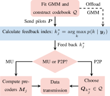
Figure 1: Flowchart of the proposed versatile feedback scheme. Red (blue) colored nodes are processed at the BS (MTs).

VI Baseline Channel Estimators

Conventionally, the DL channel is estimated firstly at each MT and subsequently, the best fitting codebook entry is determined. Thus, in this section, we present the baseline channel estimators which we consider in our simulations. Since channel estimation takes place at each MT separately, we present the estimators from a MT perspective and drop the index $j$ in the following for brevity. The mean squared error (MSE)-optimal channel estimate for the model (4) is given by the conditional mean estimator (CME) $\operatorname{E}[\bm{h}\mid\bm{y}]$, cf., e.g., [51, Section 8.1]. However, the true channel PDF is generally not known and, therefore, the CME can generally not be calculated analytically. Even if the true channel PDF was known, the CME $\operatorname{E}[\bm{h}\mid\bm{y}]$ might still not have an analytic expression.

In this work, we use the recently proposed GMM-based channel estimator $\hat{\bm{h}}_{\text{GMM}}$, see (24), from [21] as a baseline. The GMM-based channel estimator is proven to asymptotically converge to the optimal CME as the number of GMM components $K$ is increased, with the restriction that $\bm{A}$ is invertible, see (4). In our case, we would have to fulfil that $n_{p}=N_{\mathrm{tx}}$. However, even if $\bm{A}$ is not invertible ($n_{p}<N_{\mathrm{tx}}$) and for a moderate number for $K$, the GMM-based channel estimator is a powerful estimator as shown in [21]. The GMM-based channel estimator utilizes the same GMM as found in Subsection III-B. In particular, the MT can use the GMM (obtained through offloading) to estimate the channel by evaluating:

$$\hat{\bm{h}}_{\text{GMM}}(\bm{y})=\sum_{k=1}^{K}p(k\mid\bm{y})\hat{\bm{h}}_{\text{LMMSE},k}(\bm{y})$$ (24)

with the responsibilities $p(k\mid\bm{y})$ from (13) and

$$\hat{\bm{h}}_{\text{LMMSE},k}(\bm{y})=\bm{C}_{k}\bm{A}^{\operatorname{H}}(\bm{A}\bm{C}_{k}\bm{A}^{\operatorname{H}}+{\bm{\Sigma}})^{-1}(\bm{y}-\bm{A}{\bm{\mu}}_{k})+{\bm{\mu}}_{k}.$$ (25)

Accordingly, the estimator $\hat{\bm{h}}_{\text{GMM}}$ is given by a weighted sum of $K$ linear minimum mean square error (LMMSE) estimators—one for each component. The weights $p(k\mid\bm{y})$ are the probabilities that the current observation $\bm{y}$ corresponds to the $k$th component.

Another baseline is the LMMSE estimator, which utilizes the sample covariance matrix $\bm{C}_{s}=\frac{1}{M}\sum_{m=1}^{M}\bm{h}_{m}\bm{h}_{m}^{\operatorname{H}}$, which is calculated using the same set of training samples to fit the GMM, and calculate channel estimates as (cf. [15, 21]):

$$\hat{\bm{h}}_{\text{LMMSE}}=\bm{C}_{s}\bm{A}^{\operatorname{H}}(\bm{A}\bm{C}_{s}\bm{A}^{\operatorname{H}}+{\bm{\Sigma}})^{-1}\bm{y}.$$ (26)

Lastly, compressive sensing approaches commonly assume that the channel exhibits a certain structure: $\bm{h}\approx\bm{D}\bm{t}$, where $\bm{D}=\bm{D}_{\text{rx}}\otimes(\bm{D}_{\text{tx,h}}\otimes\bm{D}_{\text{tx,v}})$ is a dictionary with oversampled DFT matrices $\bm{D}_{\text{rx}}$, $\bm{D}_{\text{tx,h}}$, and $\bm{D}_{\text{tx,v}}$ (cf., e.g., [52]), because we have a URA at the BS and a ULA at the MT. A compressive sensing algorithm like orthogonal matching pursuit (OMP) [53] can now be used to obtain a sparse vector $\bm{t}$, and the estimated channel is then given by

$$\hat{\bm{h}}_{\text{OMP}}=\bm{D}\bm{t}.$$ (27)

Since the sparsity order is not known, but the algorithm’s performance crucially depends on it, we use a genie-aided approach to obtain a bound on the performance of the algorithm. Specifically, we use the true channel (perfect CSI knowledge) to choose the optimal sparsity order.

VII Complexity Analysis

The responsibilities in (13) are calculated by evaluating Gaussian densities. Since the GMM’s covariance matrices and mean vectors do not change for different observations, the inverse and the determinant of the densities can be pre-computed. Therefore, the online evaluation of the responsibilities $p(k\mid\bm{y})$ in (13) is dominated by matrix-vector multiplications and has a complexity of $\mathcal{O}(L^{2})$ per GMM component, with $L=N_{\mathrm{rx}}n_{p}$.

Correspondingly, determining the feedback using the GMM via (14) has a complexity of $\mathcal{O}(KN_{\mathrm{rx}}^{2}n_{p}^{2})$. Recall that in this case, no channel estimation needs to be conducted. One huge advantage is, that the complexity does not scale with the number of transmit antennas $N_{\mathrm{tx}}$. This is particularly beneficial if the BS is equipped with many antennas, as it is the case for massive MIMO systems. Moreover, the proposed method allows for parallelization with respect to the number of components $K$, i.e., all of the $K$ responsibilities can be evaluated in parallel.

When using the conventional approach of first estimating the channel and then searching for the best codebook entry, the complexity depends on the channel estimation complexity and the complexity of the selection method from (9). Among all considered conventional approaches, the GMM estimator from (24) in combination with the selection method that maximizes the rate expression from (9) performed best in our simulations, cf. Section VIII. Evaluating the GMM estimator from (24) has a complexity of $\mathcal{O}(KN_{\mathrm{rx}}^{2}n_{p}^{2}+KN_{\mathrm{rx}}^{2}N_{\mathrm{tx}}n_{p})$, due to the calculation of the responsibilities $p(k\mid\bm{y})$ and the evaluation of the LMMSE filters from (25) [21]. The responsibilities $p(k\mid\bm{y})$ from (13) to determine the feedback using the GMM according to (14) are the same responsibilities which are needed to evaluate the GMM estimator from (24). Evaluating the GMM estimator further requires the calculation of the LMMSE filters from (25). Thus, in terms of floating-point operations (FLOPS) our proposed method from (14) is in any case of lower complexity for the MT as compared to evaluating the GMM estimator from (24). In addition to that, with the conventional approach, the estimated channel has to be further processed to a feedback index by evaluating (9). The complexity of this selection method is $\mathcal{O}(KN_{\mathrm{tx}}N_{\mathrm{rx}}^{2}+KN_{\mathrm{rx}}^{3})$, when exploiting the QR decomposition [54, Section 5.2].

This complexity analysis also holds for the multi-user case since the feedback is determined at each MT separately by conducting similar steps, i.e., by first estimating the channel and then evaluating either (18) in the case of random codebooks, or (20) in the case of the directional codebook.

Kronecker Approximation for Reducing the Offloading Amount: In order for a MT to be able to compute feedback indices, the parameters of the GMM $f_{\bm{h}}^{(K)}$ need to be offloaded to the MT upon entering the BS’ coverage area. As demonstrated in a numerical example in Table I, the number of GMM parameters can be quite large. This is mainly due to the large number of parameters of the GMM’s covariance matrices. In order to reduce the number of GMM parameters, we can incorporate model-based insights without influencing the online computational complexity. For spatial correlation scenarios, a well-known assumption is that the scattering in the vicinity of the transmitter and receiver are independent of each other, cf. [55]. Similarly, as in [21], we use this assumption to constrain the GMM covariance matrices to a Kronecker factorization with fewer parameters, i.e., we construct a GMM consisting of covariance matrices of the form $\bm{C}_{k}=\bm{C}_{\text{tx},k}\otimes\bm{C}_{\text{rx},k}$. Thus, instead of fitting a single unconstrained GMM with $N\times N$-dimensional covariances, a transmit-side (receive-side) GMM with $N_{\text{tx}}\times N_{\text{tx}}$ ($N_{\text{rx}}\times N_{\text{rx}}$)-dimensional covariances and $K_{\text{tx}}$ ($K_{\text{rx}}$) components is fitted. Thereafter, a $K=K_{\mathrm{tx}}K_{\mathrm{rx}}$-components GMM with $N\times N$-dimensional covariances is obtained by combinatorially computing all Kronecker products of the respective transmit- and receive-side covariance matrices. It was observed in [21] that the Kronecker GMM performs almost equally well as compared to the unconstrained GMM. The advantages of the Kronecker GMM are a lower offline training complexity, the ability to parallelize the fitting process, and the need for fewer training samples since the Kronecker GMM has much fewer parameters.

Name	Online Complexity	Covariance Parameters	$(N_{\mathrm{tx}},N_{\mathrm{rx}})=(32,16)$, $(K_{\mathrm{tx}},K_{\mathrm{rx}})=(16,4)$
Full	$\mathcal{O}(KN_{\mathrm{rx}}^{2}n_{p}^{2})$	$\frac{1}{2}KN(N+1)$	$8.4\cdot 10^{6}$
Kronecker	$\mathcal{O}(KN_{\mathrm{rx}}^{2}n_{p}^{2})$	$\frac{1}{2}K_{\mathrm{rx}}N_{\mathrm{rx}}(N_{\mathrm{rx}}+1)$ $+\frac{1}{2}K_{\mathrm{tx}}N_{\mathrm{tx}}(N_{\mathrm{tx}}+1)$	$9\cdot 10^{3}$

TABLE I: Analysis of the number of parameters of the (structured) GMM.

Table I illustrates exemplarily the difference in the number of GMM covariance parameters (taking symmetries into account), where we plug in the simulation parameters of one of the settings with $B=6$, which we consider in Section VIII. We can see that, with the Kronecker GMM, the number of parameters that need to be offloaded is drastically reduced. For the remaining settings considered in Section VIII, the reduction factors due to the Kronecker GMM are in the order of approximately $10^{2}$ to $10^{3}$. For this reason, we solely consider the Kronecker GMM in Section VIII.

VIII Simulation Results

With trends towards massive MIMO, both the BS and the MTs are equipped with many antennas [56]. The BS equipped with a URA has in total $N_{\mathrm{tx}}=N_{\mathrm{tx,h}}N_{\mathrm{tx,v}}$ antenna elements, with $N_{\mathrm{tx,h}}$ horizontal and $N_{\mathrm{tx,v}}$ vertical elements. At the MT, we have a ULA with $N_{\mathrm{rx}}$ elements. We consider $B$ feedback bits and thus $K=2^{B}$. We generate datasets with $30\cdot 10^{3}$ channels for both the UL and DL domain of the scenario described in Section II-D: $\mathcal{H}^{\text{UL}}$ and $\mathcal{H}^{\text{DL}}$. The data samples are normalized such that $\operatorname{E}[\|\bm{h}\|^{2}]=N=N_{\mathrm{tx}}N_{\mathrm{rx}}$ holds for the vectorized channels. We further set $\rho=1$, which allows us to define the SNR as $\frac{1}{\sigma_{n}^{2}}$ for all MTs, i.e., when $\sigma^{2}_{j}=\sigma^{2}_{n},\forall j\in\mathcal{J}$. We split the two sets $\mathcal{H}^{\text{UL}}$ and $\mathcal{H}^{\text{DL}}$ into a training set with $M=20\cdot 10^{3}$ samples, and the remaining samples constitute an evaluation set, viz., $\mathcal{H}_{\text{train}}^{\text{UL}},\mathcal{H}_{\text{eval}}^{\text{UL}},\mathcal{H}_{\text{train}}^{\text{DL}},\ \text{and}\ \mathcal{H}_{\text{eval}}^{\text{DL}}.$ The following transmit strategies are always evaluated on $\mathcal{H}_{\text{eval}}^{\text{DL}}$, i.e., in the DL domain. When we fit the GMM based on $\mathcal{H}_{\text{train}}^{\text{UL}}$, we transpose all elements of the set to emulate a DL, cf. [8, 15, 17].

VIII-A Point-to-point MIMO

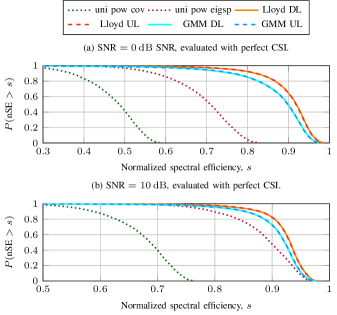
Figure 2: Empirical cCDFs of the normalized (by the optimal transmit strategy) spectral efficiencies achieved with different codebooks and transmit strategies evaluated with perfect CSI, for a system with $N_{\mathrm{tx}}=32$, $N_{\mathrm{rx}}=16$, and $B=6$ bits.

In the single-user case, we depict the normalized spectral efficiency (nSE) as performance measure. The spectral efficiency achieved with a given transmit covariance matrix is normalized by the spectral efficiency achieved with the optimal transmit covariance matrix, which is given by decomposing the channel into $N_{\mathrm{rx}}$ parallel streams and employing water-filling [38]. The empirical cCDF $P(\text{nSE}>s)$ of the normalized spectral efficiency, corresponds to the empirical probability that nSE exceeds a specific value $s$.

We consider the following baseline transmit strategies: The curves labeled “uni pow cov” represent uniform power allocation where the transmit covariance matrix is given by $\bm{Q}=\frac{\rho}{N_{\mathrm{tx}}}\mathbf{I}$. In this case, no CSI knowledge or codebook is used. Moreover, “uni pow eigsp” corresponds to the transmit strategy where a transmit covariance matrix is calculated by allocating equal power on the eigenvectors of the channel. That is, the channel is decomposed into $N_{\mathrm{rx}}$ parallel streams and $\frac{\rho}{N_{\mathrm{rx}}}$ power is allocated to each stream. Note that this approach is infeasible because the BS would require full knowledge of the DL channel (or its eigenvectors).

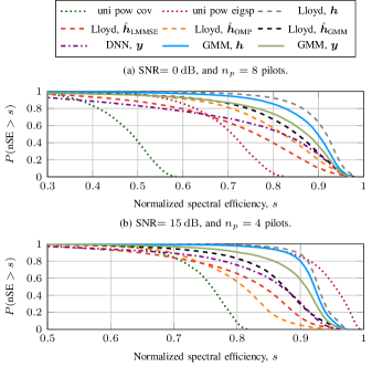
Figure 3: Empirical cCDFs of the normalized (by the optimal transmit strategy) spectral efficiencies achieved with different codebooks and transmit strategies evaluated for a system with $N_{\mathrm{tx}}=32$, $N_{\mathrm{rx}}=16$, different SNRs, different number of pilots $n_{p}$, and $B=6$ bits.

In the following, the simulation parameters are $N_{\mathrm{tx}}=32$ ($N_{\mathrm{tx,h}}=8,N_{\mathrm{tx,v}}=4$), $N_{\mathrm{rx}}=16$ and $B=6$ bits, thus $K=64$ ($K_{\text{tx}}=16$, $K_{\text{rx}}=4$). In Fig. 2(a), we set the $\text{SNR}=$0\text{\,}\mathrm{d}\mathrm{B}$$. The conventional codebook construction approach (cf. Section III-A) is denoted by “Lloyd UL/DL”, depending on whether $\mathcal{H}_{\text{train}}^{\text{UL}}$ or $\mathcal{H}_{\text{train}}^{\text{DL}}$ is used as training data to construct the codebooks, respectively. With these approaches, the codebook is known to the BS and the MT and, additionally, perfect CSI is assumed at the MT. Each MT then selects the best possible codebook entry by evaluating (9). We can observe that, using DL or UL training data, results in approximately the same performance. The proposed codebook construction and encoding scheme is denoted by “GMM UL/DL”, where we either use $\mathcal{H}_{\text{train}}^{\text{UL}}$ or $\mathcal{H}_{\text{train}}^{\text{DL}}$ as training data to fit the GMM and to construct the codebook as described in Section III-B. With our proposed approach, the knowledge of the codebook at the MT is not required. After offloading the GMM to the MT and given perfect CSI knowledge, the MT can then determine the feedback index by evaluating (15). Again, using DL or UL training data results in approximately the same performance, which is in accordance with the findings from [8, 15, 17]. The proposed GMM approach performs slightly worse than the Lloyd clustering approach, which is a consequence of the perfect CSI assumption. In Fig. 2(b), we set $\text{SNR}=$10\text{\,}\mathrm{d}\mathrm{B}$$, and observe similar results.

However, assuming perfect CSI at the MT is not feasible. In the following, we consider imperfect CSI, i.e., systems with reduced pilot overhead ($n_{p}\leq N_{\mathrm{tx}}$). In the remainder, we consider UL training data exclusively. Thus, we omit writing “UL” in the legend from now on.

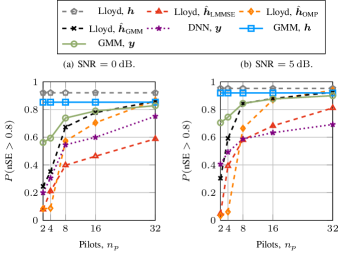
Figure 4: The probability that the nSE of a certain transmit strategy exceeds $s=80\%$ of the optimal transmit strategy’s spectral efficiency for a varying number of pilots, for a system with $N_{\mathrm{tx}}=32$, $N_{\mathrm{rx}}=16$, and $B=6$ bits.

In Fig. 3(a), the $\text{SNR}=$0\text{\,}\mathrm{d}\mathrm{B}$$ and we have $n_{p}=8$. We depict results for the conventional Lloyd codebook construction approach (cf. Section III-A), where we first estimate the channel either via OMP (27), the LMMSE approach (26), or via the GMM estimator (24), and then select a transmit covariance matrix by evaluating (9) given the estimated channel: “Lloyd, $\hat{\bm{h}}_{\text{OMP}}$”, “Lloyd, $\hat{\bm{h}}_{\text{LMMSE}}$”, or “Lloyd, $\hat{\bm{h}}_{\text{GMM}}$”, respectively. Moreover, we compare to the SNR-independent DNN approach from [8], denoted by “DNN $\bm{y}$”, where a classifier is employed to directly map the observation to a feedback index that specifies an element from the Lloyd codebook. During the training phase, the DNN was provided with input-output pairs $\{(\bm{Y}_{m}=\operatorname{unvec}(\bm{y}_{m}),k^{\star}_{m})\}_{m=1}^{M}$ for an SNR range of $0\text{\,}\mathrm{d}\mathrm{B}$ to $25\text{\,}\mathrm{d}\mathrm{B}$, with $5\text{\,}\mathrm{d}\mathrm{B}$ steps. We employ random search [57] to determine the hyperparameters of the DNN. The DNN consists of $D_{\text{CM}}$ convolutional modules, which comprise a convolutional layer, a batch normalization, and an activation function, where $D_{\text{CM}}$ is randomly chosen from the range $[2,5]$. Each of the convolutional layers consists of $D_{\text{K}}$ kernels, where $D_{\text{K}}$ is randomly chosen within $[16,64]$. After a subsequent two-dimensional max-pooling, the features are flattened, and a fully connected layer is employed with an output dimension of $K$. Depending on the randomly drawn parameters, the number of DNN parameters is at least the same as or even higher than the number of GMM parameters, and increases with the number of pilots. Moreover, note that a separate DNN per pilot configuration is needed. The complexity of the DNN approach is $\mathcal{O}(KD_{\text{K}}N_{\mathrm{rx}}n_{p})$. Further details can be found in [8]. As can be seen, estimating the channel via the GMM estimator gives the best performance when considering the conventional channel estimation-based approaches. The DNN approach, which also does not require any codebook knowledge, similar to our proposed GMM-based feedback scheme, achieves comparable performance as “Lloyd, $\hat{\bm{h}}_{\text{OMP}}$” or “Lloyd, $\hat{\bm{h}}_{\text{LMMSE}}$”. In contrast, with the proposed approach (cf. Section III-B) denoted by “GMM, $\bm{y}$”, where we bypass channel estimation and directly evaluate (14) for determining a feedback index, we achieve even better performance as compared to any of the conventional approaches. With the curves “Lloyd, $\bm{h}$” and “GMM, $\bm{h}$”, we depict the results for the utopian case of assuming perfect CSI knowledge at the MT. Although the Lloyd approach performs well if perfect CSI is available at the MT, the performance suffers significantly from CSI imperfections (due to noise and low pilot overhead). In contrast, the proposed GMM-based feedback scheme is superior in case of imperfect CSI available at the MT, which resembles practical system deployments. A similar observation can also be made in Fig. 3(b), where the $\text{SNR}=$15\text{\,}\mathrm{d}\mathrm{B}$$ and we only have $n_{p}=4$ pilots.

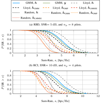
Figure 5: Empirical cCDFs of the sum-rate ($N_{\mathrm{tx}}=16$, $N_{\mathrm{rx}}=4$, and $J=4$ MTs) achieved with different feedback approaches and precoding techniques for different SNRs, different number of pilots $n_{p}$, and $B=6$ bits.

In Fig. 4(a), we set $\text{SNR}=$0\text{\,}\mathrm{d}\mathrm{B}$$ and in Fig. 4(b), we have $\text{SNR}=$5\text{\,}\mathrm{d}\mathrm{B}$$, where we fix $s=0.8$, thus, we consider $P(\text{nSE}>0.8)$ for a varying number of pilots $n_{p}$. We see that our proposed low-complexity feedback scheme is beneficial in the low number of pilots regime and outperforms the conventional approaches, which either require both channel estimation and the feedback evaluation via (9) or the DNN-based approach.

VIII-B Multi-user MIMO

In this subsection, we present simulation results for the multi-user setup and depict the sum-rate as performance measure, which is given by $\sum_{j=1}^{J}R_{j}^{\text{inst}}$, cf. (2). We depict the results for $2{,}500$ constellations, where for each constellation, we draw $J$ MTs randomly from our evaluation set $\mathcal{H}_{\text{eval}}^{\text{DL}}$. The empirical cCDF $P(\text{SR}>s)$ of the sum-rate, is used to depict the empirical probability that the sum-rate (SR) exceeds a specific value $s$.

In the following, with “GMM, $\bm{h}$” and “GMM, $\bm{y}$” we denote the cases, where either perfect CSI $\bm{h}_{j}$ is assumed or the observations $\bm{y}_{j}$ are used at each MT $j$ to determine a feedback index using the GMM feedback encoding approach, cf. (21). We omit the index $j$ in the legend for notational convenience. The channel of each MT is then represented by the subspace information extracted from the high-SNR GMM codebook, cf. Section IV-B. With “Lloyd, $\bm{h}$”, “Lloyd, $\hat{\bm{h}}_{\text{GMM}}$”, “Lloyd, $\hat{\bm{h}}_{\text{OMP}}$”, and “Lloyd, $\hat{\bm{h}}_{\text{LMMSE}}$”, or with “Random, $\bm{h}$”, “Random, $\hat{\bm{h}}_{\text{GMM}}$”, “Random, $\hat{\bm{h}}_{\text{OMP}}$”, and “Random, $\hat{\bm{h}}_{\text{LMMSE}}$”, we denote the cases where either perfect CSI is assumed at each MT, or the channel is firstly estimated at each MT and then the index of the best fitting subspace entry of the high-SNR Lloyd codebook or of the random codebook, is fed back from each MT to the BS, cf. Sections IV-B and IV-A.

The above mentioned approaches are evaluated using either RBD, RCI, or the iterative WMMSE to jointly design the precoders $\bm{M}_{j},\ \forall j\in\mathcal{J}$. In case of RBD and RCI, the used regularization factor is $\frac{JN_{\mathrm{rx}}\sigma_{n}^{2}}{\rho}$, and the precoders are normalized to satisfy the transmit power constraint, cf. [29, 30, 31]. In the case of the iterative WMMSE, we use [34, Algorithm 1]. Additionally, with “GMM samples, $\bm{h}$” and “GMM samples, $\bm{y}$”, we denote the cases where we generate samples which represent each MT’s distribution using the GMM and feed them to the SWMMSE algorithm, cf. Section IV-C. In all iterative approaches, we set $I_{\max}=300$ iterations.

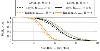
Figure 6: Empirical cCDFs of the sum-rate ($N_{\mathrm{tx}}=16$, $N_{\mathrm{rx}}=4$, and $J=4$ MTs) achieved with different feedback approaches when RBD is employed for a system with an $\text{SNR}=$10\text{\,}\mathrm{d}\mathrm{B}$$, $n_{p}=4$ pilots, and different bits $B$.

In the following, the simulation parameters are $N_{\mathrm{tx}}=16$ ($N_{\mathrm{tx,h}}=4,N_{\mathrm{tx,v}}=4$), $N_{\mathrm{rx}}=4$ and $B=6$ bits, thus $K=64$ ($K_{\text{tx}}=16$, $K_{\text{rx}}=4$). Accordingly, we have $J=4$ MTs. In Fig. 5(a), the $\text{SNR}=$5\text{\,}\mathrm{d}\mathrm{B}$$ and we have $n_{p}=8$ pilots. In this case, we use RBD in order to jointly design the precoders. We can observe that the random codebook performs worst. Even with perfect CSI assumed at the MTs, the random codebook approach cannot compete with the environment-aware approaches. The Lloyd directional codebook approach yields the best performance, if the GMM-based channel estimator from (24) is used prior to codebook entry selection. Similar to the point-to-point MIMO case, we can observe that the chosen channel estimator significantly impacts the performance. That is, using the LMMSE estimator from (26) or the genie OMP from (27) yield worse results as compared to the GMM-based channel estimator. Furthermore, our proposed GMM-based feedback approach (“GMM, $\bm{y}$”) even outperforms the best conventional approach (“Lloyd, $\hat{\bm{h}}_{\text{GMM}}$”). A similar behavior can be observed in Fig. 5(b), where we increased the SNR to $10\text{\,}\mathrm{d}\mathrm{B}$ and decreased the number of pilots $n_{p}=4$, and use RCI in order to jointly design the precoders.

In the following two figures (Fig. 6 and Fig. 7) we restrict our analysis to RBD as the precoder design algorithm for sake of brevity. The purpose of the next two figures is to quantify the performance gains obtained with our proposed approach from different perspectives. In particular, in Fig. 6 we have $\text{SNR}=$10\text{\,}\mathrm{d}\mathrm{B}$$ and $n_{p}=4$, and we consider systems with $B=4$ bits, thus, $K=16$ ($K_{\text{tx}}=8$, $K_{\text{rx}}=2$), or $B=8$ bits, thus $K=256$ ($K_{\text{tx}}=32$, $K_{\text{rx}}=8$) and compare the performance of our proposed GMM-based feedback approach (“GMM, $\bm{y},B\in\{4,8\}$”) to the best performing conventional Lloyd directional codebook (“Lloyd, $\hat{\bm{h}}_{\text{GMM}},B\in\{4,8\}$”) and random codebook (“Random, $\hat{\bm{h}}_{\text{GMM}},B\in\{4,8\}$”) approaches, which use the GMM-based channel estimator in the channel estimation phase. We can observe that our proposed feedback approach is superior to the conventional methods. In particular, our proposed feedback approach with only $B=4$ bits (“GMM, $\bm{y},B=4$”) even outperforms the conventional Lloyd directional codebook with twice as much, i.e., $B=8$, bits (“Lloyd, $\hat{\bm{h}}_{\text{GMM}},B=8$”).

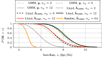
Figure 7: Empirical cCDFs of the sum-rate ($N_{\mathrm{tx}}=64$, $N_{\mathrm{rx}}=4$, and $J=16$ MTs) achieved with different feedback approaches when RBD is employed for systems with an $\text{SNR}=$5\text{\,}\mathrm{d}\mathrm{B}$$, different number of pilots $n_{p}$, and $B=6$ bits.

In Fig. 7, we consider a system with more transmit antennas and, accordingly, more MTs. The simulation parameters are $N_{\mathrm{tx}}=64$ ($N_{\mathrm{tx,h}}=8,N_{\mathrm{tx,v}}=8$), $N_{\mathrm{rx}}=4$, and $B=6$ bits, thus, $K=64$ ($K_{\text{tx}}=16$, $K_{\text{rx}}=4$), and the $\text{SNR}=$5\text{\,}\mathrm{d}\mathrm{B}$$. Accordingly, we have $J=16$ MTs. This time, we depict the performances for a varying number of pilots $n_{p}$. For a fixed number of pilots $n_{p}$, our proposed approach (“GMM, $\bm{y},n_{p}\in\{2,6,12\}$”) outperforms the conventional approaches (“Lloyd, $\hat{\bm{h}}_{\text{GMM}},n_{p}\in\{2,6,12\}$” and “Lloyd, $\hat{\bm{h}}_{\text{OMP}},n_{p}=12$”). Moreover, with only $n_{p}=2$ pilots, our proposed feedback approach (“GMM, $\bm{y},n_{p}=2$”), almost achieves the same performance as the conventional approaches, which require $n_{p}=6$ pilots in the case of “Lloyd, $\hat{\bm{h}}_{\text{GMM}},n_{p}=6$”, or even $n_{p}=12$ in the case of “Lloyd, $\hat{\bm{h}}_{\text{OMP}},n_{p}=12$” (i.e., the MTs are unaware of the GMM and use the OMP channel estimator). If random codebooks are used, the performance with even a large pilot overhead, i.e. $n_{p}=64$ pilots, is poor (“Random, $\hat{\bm{h}}_{\text{GMM}},n_{p}=64$”). Thus, with our proposed approach, systems with lower pilot overhead can be deployed, which would inherently increase the system throughput. Additionally, with fewer pilots, the complexity of determining the feedback index at the MTs with the proposed GMM-based approach decreases, cf. Section VII.

So far, we have only considered non-iterative precoding algorithms, i.e., RBD and RCI. In the remainder, we will focus our analysis on the iterative WMMSE and the SWMMSE precoding techniques. Due to the exclusive usage of channel directional information, i.e., no channel magnitude information is fed back to the BS, as in [5] (cf. Section IV-A), in case of random codebooks, or the Lloyd directional codebook from Section IV-B, or the GMM directional codebook from Section IV-B, changing the number of streams $d$ impacts the overall sum-rate which can be achieved using the iterative WMMSE. In fact, we observed that depending on the SNR, the number of pilots $n_{p}$, the chosen channel estimator (for the conventional approaches), and the selected codebook, the performance can be improved by varying $d\in\{1,2,\cdots,N_{\mathrm{rx}}\}$, and then setting $d$ to the value which gives the best average performance. In a practical deployment, the parameter $d$ can be pre-adjusted in the offline phase at the BS by emulating a DL system (for example using the set $\mathcal{H}_{\text{eval}}^{\text{UL}}$). However, things are different with the SWMMSE. There we observed that setting $d=N_{\mathrm{rx}}$ always yields the best performance. Intuitively, due to the sampling involved in the design procedure of the SWMMSE, (average) channel magnitude information is provided to and exploited by the SWMMSE algorithm, which enables the SWMMSE to adjust the stream powers accordingly.

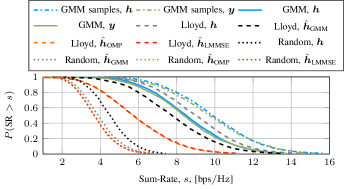
Figure 8: Empirical cCDFs of the sum-rate ($N_{\mathrm{tx}}=16$, $N_{\mathrm{rx}}=4$, and $J=4$ MTs) achieved with different feedback approaches when the iterative WMMSE or the SWMMSE are employed, for a system with an $\text{SNR}=$5\text{\,}\mathrm{d}\mathrm{B}$$, $n_{p}=8$ pilots, and $B=6$ bits.

In the remainder, the simulation parameters are again $N_{\mathrm{tx}}=16$ ($N_{\mathrm{tx,h}}=4,N_{\mathrm{tx,v}}=4$), $N_{\mathrm{rx}}=4$, yielding $J=4$ MTs, and $B=6$ bits, thus, $K=64$ ($K_{\text{tx}}=16$, $K_{\text{rx}}=4$). In Fig. 8, the $\text{SNR}=$5\text{\,}\mathrm{d}\mathrm{B}$$ and we have $n_{p}=8$ pilots. This is the same simulation setting as in Fig. 5(a), where RBD was used in order to design the precoders. By comparing Fig. 8 and Fig. 5(a), we can conclude that by using the iterative precoding techniques, the performances of the conventional and the proposed feedback approaches are improved tremendously. We can observe, that also in the case of iterative precoding techniques, the random codebook approach performs worst. Also in this case, the Lloyd directional codebook approach yields the best performance, if the GMM-based channel estimator from (24) is used prior to codebook entry selection whereas using the LMMSE estimator from (26) or the genie OMP from (27) deteriorates the performance. Furthermore, our proposed low-complexity GMM-based feedback approach (“GMM, $\bm{y}$”) again outperforms the best conventional approach (“Lloyd, $\hat{\bm{h}}_{\text{GMM}}$”). With our generative modeling-based approach from Section IV-C, i.e., the SWMMSE with samples generated by the GMM, denoted by “GMM samples, $\bm{h}$” or “GMM samples, $\bm{y}$”, we even outperform the performance bound of the Lloyd directional codebook approach (which uses the iterative WMMSE) with perfect CSI assumed at the MTs (“Lloyd, $\bm{h}$”). This shows the great potential of the generative modeling ability of the GMM.

In Fig. 9, we still consider a setting with $n_{p}=8$ pilots but vary the SNR. We depict the sum-rate averaged over all constellations. We can see, that our proposed GMM-based feedback approach, with either exploiting directional information (“GMM, $\bm{y}$”) or the generative modeling-based approach (“GMM samples, $\bm{y}$”) outperform the conventional approaches. We can observe, that in this case, up to an SNR of $\approx$15\text{\,}\mathrm{d}\mathrm{B}$$, the generative modeling-based method performs better, and for larger SNR values, the directional approach is superior. This is illustrated by the arrows in Fig. 9. Thus, the results suggest that jointly designing the precoders by solving the ergodic sum-rate maximization problem from (22) by utilizing the SWMMSE, is beneficial for low to medium SNR values, and the directional approach, which exploits the iterative WMMSE, is superior for larger SNR values.

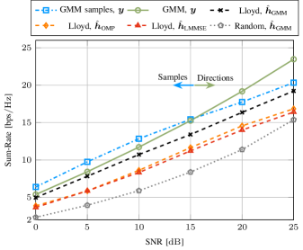
Figure 9: The average sum-rate ($N_{\mathrm{tx}}=16$, $N_{\mathrm{rx}}=4$, and $J=4$ MTs) over the SNR achieved with different feedback approaches when the iterative WMMSE or the SWMMSE are employed, for $n_{p}=8$ pilots, and $B=6$ bits.

This observation is also supported by the results in Fig. 10, where we depict the performances of our proposed approaches “GMM, $\bm{y}$” and “GMM samples, $\bm{y}$” and compare them to the best performing conventional method “Lloyd, $\hat{\bm{h}}_{\text{GMM}}$”, and the random codebook-based approach which uses the OMP estimator “Random, $\hat{\bm{h}}_{\text{OMP}}$” (i.e., no environment awareness) for a varying SNR and $n_{p}\in\{2,8,16\}$. There, dotted curves represent $n_{p}=2$, dashed curves $n_{p}=8$, and solid curves $n_{p}=16$ pilots. The approaches with no environment awareness, i.e., “Random, $\hat{\bm{h}}_{\text{OMP}}$” perform worst. Both of our proposed approaches, i.e., “GMM, $\bm{y}$” and “GMM samples, $\bm{y}$”, with only $n_{p}=2$ pilots, outperform the conventional “Lloyd, $\hat{\bm{h}}_{\text{GMM}}$” approach with four times more, i.e., $n_{p}=8$, pilots. When the number of pilots is equal to the number of transmit antennas (large pilot overhead), i.e., $n_{p}=N_{\mathrm{tx}}=16$, our proposed approaches which solely require the GMM at the MTs, at least can compete with the conventional “Lloyd, $\hat{\bm{h}}_{\text{GMM}}$” approach, which requires both the GMM and the Lloyd directional codebook at each MT. For SNRs up to about $15\text{\,}\mathrm{d}\mathrm{B}$ our proposed generative modeling-based approach even outperforms the conventional method based on the Lloyd directional codebook.

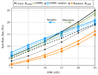
Figure 10: The average sum-rate ($N_{\mathrm{tx}}=16$, $N_{\mathrm{rx}}=4$, and $J=4$ MTs) over the SNR achieved with different feedback approaches using the iterative WMMSE or the SWMMSE, for different number of pilots $n_{p}$ (dotted: $n_{p}=2$, dashed: $n_{p}=8$, solid: $n_{p}=16$), and $B=6$ bits.

Finally, in Fig. 11, we present how the sum-rate evolves over the number of iterations in the case of the iterative WMMSE (solid curves), or over the number of drawn samples (per MT) in the case of the SWMMSE (dashed curves) for a setting with an $\text{SNR}=$5\text{\,}\mathrm{d}\mathrm{B}$$ and $n_{p}=8$ pilots. In comparison, we depict the performance of the case, where we applied RBD (dotted curves) in order to jointly design the precoders. Note that since RBD is a non-iterative approach, the respective curves are constant over the iterations. We can observe that in the case of random codebooks (“Random, $\hat{\bm{h}}_{\text{GMM}}$”) the performance gains achieved by using the iterative WMMSE, compared to using RBD, are relatively small. In contrast, using the Lloyd (“Lloyd, $\hat{\bm{h}}_{\text{GMM}}$”) or GMM (“GMM, $\bm{y}$”) directional codebook approaches, we obtain huge performance gains when we use the iterative precoding techniques. In these cases, already a small number of iterations is enough to reach the performance maximum. Interestingly, a small overshoot can be observed. This artefact is possibly due to the fact that the iterative WMMSE is designed for perfect CSI, but here we are restricted to using directional information due to the limited feedback. In contrast, when we use the generative modeling-based approach (“GMM samples, $\bm{y}$”) we can observe that the performance steadily improves over the number of drawn samples. We observed this behavior consistently for different SNR values and numbers of pilots.

IX Conclusion

In this work, we have investigated a novel GMM-based feedback scheme for FDD systems. In particular, we proposed to use a GMM for codebook construction, feedback encoding, and as a generator, which provides statistical information about the channels of the MTs to the BS. The proposed scheme exhibits lower computational complexity as compared to state-of-the-art approaches, and even allows for parallelization at the MTs. Moreover, the proposed scheme stands out through its versatility. That is, given the feedback information of the MTs at the BS, it is flexible in deciding for the single-user or the multi-user transmission mode. The versatility is even more pronounced through a convenient adaption at the MTs to any desired SNR and pilot configuration without retraining the GMM. This is a huge advantage as compared to existing end-to-end DNN approaches, which do not provide this versatility. Numerical results have demonstrated that the proposed feedback scheme outperforms conventional methods, especially in configurations with reduced pilot overhead. The achieved performance gains of the proposed scheme can be leveraged to deploy systems with lower pilot overhead or even fewer feedback bits as compared to state-of-the-art methods.

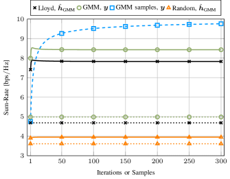
Figure 11: The average sum-rate ($N_{\mathrm{tx}}=16$, $N_{\mathrm{rx}}=4$, and $J=4$ MTs) over the number of iterations/samples achieved with different feedback approaches and precoding techniques (dotted: RBD (remains constant, since non-iterative), dashed: SWMMSE, solid: WMMSE) for a system with an $\text{SNR}=$5\text{\,}\mathrm{d}\mathrm{B}$$, $n_{p}=8$ pilots, and $B=6$ bits.

References

- [1] N. Turan, M. Koller, B. Fesl, S. Bazzi, W. Xu, and W. Utschick, “GMM-based codebook construction and feedback encoding in FDD systems,” in 56th Asilomar Conf. Signals, Syst., and Comput., 2022, pp. 37–42.
- [2] E. Björnson, L. Sanguinetti, H. Wymeersch, J. Hoydis, and T. L. Marzetta, “Massive MIMO is a reality–What is next? five promising research directions for antenna arrays,” Digit. Signal Process., vol. 94, pp. 3 – 20, 2019.
- [3] D. J. Love, R. W. Heath, V. K. N. Lau, D. Gesbert, B. D. Rao, and M. Andrews, “An overview of limited feedback in wireless communication systems,” IEEE J. Sel. Areas Commun., vol. 26, no. 8, pp. 1341–1365, 2008.
- [4] V. Lau, Y. Liu, and T.-A. Chen, “On the design of MIMO block-fading channels with feedback-link capacity constraint,” IEEE Trans. Commun., vol. 52, no. 1, pp. 62–70, 2004.
- [5] N. Ravindran and N. Jindal, “Limited feedback-based block diagonalization for the MIMO broadcast channel,” IEEE J. Sel. Areas Commun., vol. 26, no. 8, pp. 1473–1482, 2008.
- [6] E. Björnson, E. G. Larsson, and T. L. Marzetta, “Massive MIMO: ten myths and one critical question,” IEEE Commun. Mag., vol. 54, no. 2, pp. 114–123, 2016.
- [7] J. Jang, H. Lee, S. Hwang, H. Ren, and I. Lee, “Deep learning-based limited feedback designs for MIMO systems,” IEEE Wireless Commun. Lett., vol. 9, no. 4, pp. 558–561, 2020.
- [8] N. Turan, M. Koller, S. Bazzi, W. Xu, and W. Utschick, “Unsupervised learning of adaptive codebooks for deep feedback encoding in FDD systems,” in 55th Asilomar Conf. Signals, Syst., Comput., 2021, pp. 1464–1469.
- [9] F. Sohrabi, K. M. Attiah, and W. Yu, “Deep learning for distributed channel feedback and multiuser precoding in FDD massive MIMO,” IEEE Trans. Wireless Commun., vol. 20, no. 7, pp. 4044–4057, 2021.
- [10] Y. Li, K. Li, L. Cheng, Q. Shi, and Z.-Q. Luo, “Digital twin-aided learning to enable robust beamforming: Limited feedback meets deep generative models,” in IEEE 22nd Int. Workshop Signal Process. Adv. Wireless Commun. (SPAWC), 2021, pp. 26–30.
- [11] J. Guo, C.-K. Wen, M. Chen, and S. Jin, “Environment knowledge-aided massive MIMO feedback codebook enhancement using artificial intelligence,” IEEE Trans. Commun., vol. 70, no. 7, pp. 4527–4542, 2022.
- [12] K. Kong, W.-J. Song, and M. Min, “Knowledge distillation-aided end-to-end learning for linear precoding in multiuser MIMO downlink systems with finite-rate feedback,” IEEE Trans. Veh. Technol., vol. 70, no. 10, pp. 11 095–11 100, 2021.
- [13] J. Jang, H. Lee, I.-M. Kim, and I. Lee, “Deep learning for multi-user MIMO systems: Joint design of pilot, limited feedback, and precoding,” IEEE Trans. Commun., vol. 70, no. 11, pp. 7279–7293, 2022.
- [14] W. Utschick, V. Rizzello, M. Joham, Z. Ma, and L. Piazzi, “Learning the CSI recovery in FDD systems,” IEEE Trans. Wireless Commun., 2022.
- [15] B. Fesl, N. Turan, M. Koller, M. Joham, and W. Utschick, “Centralized learning of the distributed downlink channel estimators in FDD systems using uplink data,” in 25th Int. ITG Workshop Smart Antennas (WSA), 2021.
- [16] M. Baur, V. Rizzello, N. Alvarez Prado, and W. Utschick, “Empirical evaluation of distributional shifts in FDD systems based on ray-tracing,” in 26th Int. ITG Workshop Smart Antennas (WSA) and 13th Conf. Syst., Commun., Coding (SCC), 2023.
- [17] N. Turan, M. Koller, V. Rizzello, B. Fesl, S. Bazzi, W. Xu, and W. Utschick, “On distributional invariances between downlink and uplink MIMO channels,” in 25th Int. ITG Workshop Smart Antennas (WSA), 2021.
- [18] P. Mukherjee, D. Mishra, and S. De, “Gaussian mixture based context-aware short-term characterization of wireless channels,” IEEE Trans. Veh. Technol., vol. 69, no. 1, pp. 26–40, 2020.
- [19] Y. Li, J. Zhang, Z. Ma, and Y. Zhang, “Clustering analysis in the wireless propagation channel with a variational Gaussian mixture model,” IEEE Trans. Big Data, vol. 6, no. 2, pp. 223–232, 2020.
- [20] Y. Gu and Y. D. Zhang, “Information-theoretic pilot design for downlink channel estimation in FDD massive MIMO systems,” IEEE Trans. Signal Process., vol. 67, no. 9, pp. 2334–2346, 2019.
- [21] M. Koller, B. Fesl, N. Turan, and W. Utschick, “An asymptotically MSE-optimal estimator based on Gaussian mixture models,” IEEE Trans. Signal Process., vol. 70, pp. 4109–4123, 2022.
- [22] T. T. Nguyen, H. D. Nguyen, F. Chamroukhi, and G. J. McLachlan, “Approximation by finite mixtures of continuous density functions that vanish at infinity,” Cogent Math. Statist., vol. 7, no. 1, p. 1750861, 2020.
- [23] I. Goodfellow, J. Pouget-Abadie, M. Mirza, B. Xu, D. Warde-Farley, S. Ozair, A. Courville, and Y. Bengio, “Generative adversarial nets,” in Proc. Adv. Neural Inf. Process. Syst., 2014, pp. 2672–2680.
- [24] D. P. Kingma and M. Welling, “Auto-encoding variational Bayes,” in Proc. Int. Conf. Learn. Representations (ICLR), 2014.
- [25] E. Balevi, A. Doshi, A. Jalal, A. Dimakis, and J. G. Andrews, “High dimensional channel estimation using deep generative networks,” IEEE J. Sel. Areas Commun., vol. 39, no. 1, pp. 18–30, 2021.
- [26] Y. Yang, Y. Li, W. Zhang, F. Qin, P. Zhu, and C.-X. Wang, “Generative-adversarial-network-based wireless channel modeling: Challenges and opportunities,” IEEE Commun. Mag., vol. 57, no. 3, pp. 22–27, 2019.
- [27] H. Ye, L. Liang, G. Y. Li, and B.-H. Juang, “Deep learning-based end-to-end wireless communication systems with conditional GANs as unknown channels,” IEEE Trans. Wireless Commun., vol. 19, no. 5, pp. 3133–3143, 2020.
- [28] Q. Spencer, A. Swindlehurst, and M. Haardt, “Zero-forcing methods for downlink spatial multiplexing in multiuser MIMO channels,” IEEE Trans. Signal Process., vol. 52, no. 2, pp. 461–471, 2004.
- [29] V. Stankovic and M. Haardt, “Generalized design of multi-user MIMO precoding matrices,” IEEE Trans. Wireless Commun., vol. 7, no. 3, pp. 953–961, 2008.
- [30] C. Peel, B. Hochwald, and A. Swindlehurst, “A vector-perturbation technique for near-capacity multiantenna multiuser communication-part I: channel inversion and regularization,” IEEE Trans. Commun., vol. 53, no. 1, pp. 195–202, 2005.
- [31] H. Lee, K. Lee, B. M. Hochwald, and I. Lee, “Regularized channel inversion for multiple-antenna users in multiuser MIMO downlink,” in IEEE Int. Conf. Commun., 2008, pp. 3501–3505.
- [32] S. S. Christensen, R. Agarwal, E. De Carvalho, and J. M. Cioffi, “Weighted sum-rate maximization using weighted MMSE for MIMO-BC beamforming design,” IEEE Trans. Wireless Commun., vol. 7, no. 12, pp. 4792–4799, 2008.
- [33] Q. Shi, M. Razaviyayn, Z.-Q. Luo, and C. He, “An iteratively weighted MMSE approach to distributed sum-utility maximization for a MIMO interfering broadcast channel,” IEEE Trans. Signal Process., vol. 59, no. 9, pp. 4331–4340, 2011.
- [34] Q. Hu, Y. Cai, Q. Shi, K. Xu, G. Yu, and Z. Ding, “Iterative algorithm induced deep-unfolding neural networks: Precoding design for multiuser MIMO systems,” IEEE Trans. Wireless Commun., vol. 20, no. 2, pp. 1394–1410, 2021.
- [35] M. Razaviyayn, M. S. Boroujeni, and Z.-Q. Luo, “A stochastic weighted MMSE approach to sum rate maximization for a MIMO interference channel,” in IEEE 14th Int. Workshop Signal Process. Adv. Wireless Commun. (SPAWC), 2013, pp. 325–329.
- [36] M. Razaviyayn, M. Sanjabi, and Z.-Q. Luo, “A stochastic successive minimization method for nonsmooth nonconvex optimization with applications to transceiver design in wireless communication networks,” Math. Program., vol. 157, no. 2, p. 515–545, 2016.
- [37] A. Goldsmith, Wireless Communications. Cambridge Univ. Press, 2005.
- [38] I. E. Telatar, “Capacity of multi-antenna Gaussian channels,” Eur. Trans. on Telecommun., vol. 10, pp. 585–595, 1999.
- [39] Y. Tsai, L. Zheng, and X. Wang, “Millimeter-wave beamformed full-dimensional MIMO channel estimation based on atomic norm minimization,” IEEE Trans. Commun., vol. 66, no. 12, pp. 6150–6163, 2018.
- [40] S. Jaeckel, L. Raschkowski, K. Börner, and L. Thiele, “Quadriga: A 3-d multi-cell channel model with time evolution for enabling virtual field trials,” IEEE Trans. Antennas Propag., vol. 62, no. 6, pp. 3242–3256, 2014.
- [41] S. Jaeckel, L. Raschkowski, K. Börner, L. Thiele, F. Burkhardt, and E. Eberlein, “Quadriga: Quasi deterministic radio channel generator, user manual and documentation,” Fraunhofer Heinrich Hertz Institute, Berlin, Germany, Tech. Rep. v2.2.0, 2019.
- [42] Y. Linde, A. Buzo, and R. Gray, “An algorithm for vector quantizer design,” IEEE Trans. Commun., vol. 28, no. 1, pp. 84–95, Jan. 1980.
- [43] R. Hunger, D. A. Schmidt, M. Joham, and W. Utschick, “A general covariance-based optimization framework using orthogonal projections,” in 9th Int. Workshop Signal Process. Adv. Wireless Commun. (SPAWC), 2008, pp. 76–80.
- [44] N. Turan, B. Fesl, M. Grundei, M. Koller, and W. Utschick, “Evaluation of a Gaussian mixture model-based channel estimator using measurement data,” in 2022 Int. Symp. Wireless Commun. Syst. (ISWCS), 2022, pp. 1–6.
- [45] B. Fesl, N. Turan, M. Joham, and W. Utschick, “Learning a Gaussian mixture model from imperfect training data for robust channel estimation,” IEEE Wireless Commun. Lett., 2023.
- [46] C. M. Bishop, Pattern Recognition and Machine Learning (Information Science and Statistics). Berlin, Heidelberg: Springer-Verlag, 2006.
- [47] D. Love and R. Heath, “Limited feedback unitary precoding for spatial multiplexing systems,” IEEE Trans. Inf. Theory, vol. 51, no. 8, pp. 2967–2976, 2005.
- [48] W. Santipach and M. Honig, “Asymptotic capacity of beamforming with limited feedback,” in Int. Symp. Inf. Theory. (ISIT), 2004, p. 290.
- [49] W. Dai, Y. Liu, and B. Rider, “Quantization bounds on Grassmann manifolds and applications to MIMO communications,” IEEE Trans. Inf. Theory, vol. 54, no. 3, pp. 1108–1123, 2008.
- [50] F. Mezzadri, “How to generate random matrices from the classical compact groups,” Notices American Math. Soc., vol. 54, no. 5, pp. 592 – 604, May 2007.
- [51] L. L. Scharf and C. Demeure, Statistical signal processing: detection, estimation, and time series analysis. Prentice Hall, 1991.
- [52] A. Alkhateeb, G. Leus, and R. W. Heath, “Compressed sensing based multi-user millimeter wave systems: How many measurements are needed?” in IEEE Int. Conf. Acoust., Speech Signal Process. (ICASSP), 2015, pp. 2909–2913.
- [53] M. Gharavi-Alkhansari and T. Huang, “A fast orthogonal matching pursuit algorithm,” in IEEE Int. Conf. Acoust., Speech Signal Process. (ICASSP), vol. 3, 1998, pp. 1389–1392.
- [54] G. H. Golub and C. F. van Loan, Matrix Computations, 2nd ed. Johns Hopkins University Press, 1989.
- [55] J. Kermoal, L. Schumacher, K. Pedersen, P. Mogensen, and F. Frederiksen, “A stochastic MIMO radio channel model with experimental validation,” IEEE J. Sel. Areas Commun., vol. 20, no. 6, pp. 1211–1226, 2002.
- [56] J. G. Andrews, S. Buzzi, W. Choi, S. V. Hanly, A. Lozano, A. C. K. Soong, and J. C. Zhang, “What will 5G be?” IEEE J. Sel. Areas Commun., vol. 32, no. 6, pp. 1065–1082, 2014.
- [57] J. Bergstra and Y. Bengio, “Random search for hyper-parameter optimization,” J. of Mach. Learn. Res., vol. 13, p. 281–305, Feb. 2012.