Gauge fixing and gauge correlations in noncompact Abelian gauge models

Abstract

We investigate some general properties of linear gauge fixings and gauge-field correlators in lattice models with noncompact U(1) gauge symmetry. In particular, we show that, even in the presence of a gauge fixing, some gauge-field observables (like the photon-mass operator) are not well-defined, depending on the specific gauge fixing adopted and on its implementation. Numerical tests carried out in the three-dimensional noncompact lattice Abelian Higgs model fully support the analytical results and provide further insights.

I Introduction

Some nonperturbative features of quantum field theories (QFTs) can be studied from first principles by using the lattice discretization. In this formulation the Euclidean version of the theory is regularized on a space-time lattice, and the QFT problem is mapped to a statistical-mechanics one. Continuum physics emerges as the correlation length of the statistical system diverges, i.e., close to a continuous phase transition (critical point) of the lattice system. For this strategy to be feasible, there should exist a stable fixed point of the QFT renormalization group (RG) flow, which encodes the universal properties of the critical point of the statistical system.

This approach has been extensively used to investigate for example four-dimensional non-Abelian gauge theories and QCD in particular MM_book ; DGDT_book , and the $\phi^{4}$ QFTs associated with classical and quantum phase transitions in lower-dimensional systems ZJ_book ; Pelissetto:2000ek ; Sachdev_book . Only in a few cases is it possible to carry out this strategy with full analytical control Seiler_book ; GJ_book , so that one has to rely on numerical simulations of the discretized theory.

Four-dimensional non-Abelian gauge theories are peculiar, since the existence of a fixed point of the RG flow can be shown analytically by using one-loop perturbation theory Gross:1973id ; Politzer:1973fx ; Coleman:1973sx . For typical three-dimensional QFTs this is not the case, and the fixed point, if present, is generically in the strongly coupled regime. To analytically investigate its existence and extract universal information, nonperturbative approaches are required, like the expansion in the number of components MZ-03 or the continuation in the number of dimensions obtained by resumming the $\epsilon$-expansion series Wilson:1973jj ; ZJ_book .

Three-dimensional gauge theories coupled to matter fields have features in common both with four-dimensional non-Abelian gauge theories and with three-dimensional scalar models. On the one hand, the gauge coupling of three-dimensional gauge theories has positive mass dimension (the theory is super-renormalizable), thus the energy scaling of the coupling is dictated by dimensional analysis, and asymptotic freedom is clear already at tree level. On the other hand, there is also the possibility that nontrivial fixed points exist, at which the gauge coupling does not vanish, and which are usually referred to as charged fixed points. While the asymptotically free fixed points of three-dimensional Abelian and non-Abelian gauge theories have been thoroughly investigated by numerical simulations (see, e.g., Refs. Bhanot:1980pc ; Caselle:2014eka ; Athenodorou:2018sab ; Teper:1998te ; Athenodorou:2016ebg ; Bonati:2020orj ), the case of the charged fixed points has attracted less attention until quite recently, when the existence of strongly coupled charged fixed points has been suggested to explain some peculiar critical phenomena SBSVF-04 ; Fradkin_book ; Sachdev:2018ddg ; Moessner_book .

The existence of these charged fixed points, and their critical properties, can be investigated using several complementary techniques: the $\epsilon$ expansion close to four dimensions HLM-74 ; FH-96 ; IZMHS-19 ; Das:2018qmx ; Sachdev:2018nbk ; Bonati:2021tvg ; Bonati:2021rzx ; fermioni1 ; fermioni2 ; fermioni3 , the expansion in the number of components ZJ_book ; MZ-03 ; fermioni4 and numerical simulation of lattice models. Numerical studies have recently addressed this issue in the Abelian-Higgs (AH) model, i.e., in scalar quantum electrodynamics with $N$-component scalar fields, and there is by now compelling evidence that some lattice models undergo a continuous transition related to the AH QFT charged fixed point. This has been observed for $N\gtrsim 7$ using the noncompact discretization Bonati:2020jlm ; Bonati:2022ifi and the higher-charge compact discretization Bonati:2020ssr ; Bonati:2022oez , while only first-order phase transitions have been found in other cases Pelissetto:2019zvh ; Pelissetto:2019iic ; Pelissetto:2019thf ; Bracci-Testasecca:2022mxc and for smaller $N$ values Bonati:2020jlm ; Bonati:2020ssr ; MV-08 ; KMPST-08 . For $N=2$, continuous transitions were observed Pelissetto:2019zvh ; Pelissetto:2019thf , where gauge fields play no role. Topological excitations likely play an important role for the existence of the charge fixed point; however, this point is not yet fully understood MV-04 ; MS-90 ; SP-15 ; Pelissetto:2020yas ; Bonati:2022srq .

Analytical and numerical results thus support the fact that gauge-invariant correlators are well defined beyond perturbation theory in the Abelian Higgs QFT, if a large enough number of scalar flavors is present. It is then natural to ask if gauge-dependent correlators, which play a fundamental role in the usual perturbative treatment of gauge QFTs, can be given a similar nonperturbative status.

In this work we aim to investigate this point and, more generally, to clarify how the large-distance behavior of the gauge-field correlators depends on the gauge-fixing procedure adopted. For this purpose, we study gauge correlations in the noncompact formulation of Abelian gauge models. The relations that will be derived are independent of the matter content of the theory. Moreover, they are valid in the whole phase diagram of the model, and not only on the critical lines associated with charged fixed points. In the present paper, we also add a numerical study of the behavior of the gauge-field correlations in generic points of the phase diagram of the three-dimensional Abelian-Higgs model, which provides further insights on the role of the different gauge fixings. A detailed analysis of the critical behavior is left to a forthcoming paper BPV-in-prep .

To make gauge correlation functions well-defined, it is necessary to introduce a gauge-fixing term, that completely breaks the gauge invariance of the model. In noncompact discretizations, the gauge fixing plays a crucial role, since, only in the presence of a gauge fixing, the partition function and the average values of nongauge-invariant quantities are finite. This is at variance with what happens in compact formulations, in which a gauge fixing is not necessary. Also in the absence of it, the partition function is well-defined and so are average values of nongauge invariant quantities. In particular, correlations of nongauge invariant quantities are either trivial or equivalent to gauge-invariant observables, obtained by averaging the nongauge invariant quantity over the whole (compact) group of gauge transformations Elitzur:1975im ; DeAngelis:1977su ; IZ_book . The latter equivalence does not hold in noncompact formulations, since the group of gauge transformations is not compact and therefore, averages over all gauge transformations are not defined.

Once a gauge fixing is introduced, the first point to be investigated is whether and how results for nongauge-invariant quantities depend on it. Here we consider two widely used gauge fixings, the axial and the Lorenz one. We derive general results and perform a complementary numerical study in the AH model. They both indicate that gauge correlations depend somehow on the gauge choice made. In particular, we show that the photon-mass operator is well-defined only in what we call the hard Lorenz gauge (see Sec. II). Unphysical results are obtained when using the axial gauge and the soft Lorenz gauge. The conclusions of this work should be independent of the type of matter fields considered (fermions or bosons) as they only rely on some specific features of the gauge fixing functions.

The paper is organized as follows. In Sec. II we introduce the lattice model, define the gauge fixings and the gauge observable that we will focus on. In Sec. III we derive general relations, which are independent of the nature of the matter fields, between the gauge field correlation functions in the presence of different gauge fixings. In Sec. IV we present numerical results obtained in the scalar AH model, with the purpose of determining the behavior of gauge field correlation functions in the different phases present in the model. In Sec. V we review some field-theory results for the gauge dependence of the gauge field correlation functions. Finally, in Sec. VI we draw our conclusions. In App. A, we summarize some analytic results for the pure gauge model, while in App. B we derive some general relations for the gauge-dependent part of the gauge correlation functions.

II The lattice model

We consider a noncompact Abelian gauge theory on a $d$-dimensional cubic-like lattice of size $L$, with fermionic and bosonic matter fields that we collectively indicate with $\Psi$ and $\Phi$, respectively. The gauge interaction is mediated by real fields $A_{{\bm{x}},\mu}\in\mathbb{R}$, defined on the lattice links, each link being labeled by a lattice site ${\bm{x}}$ and a positive lattice direction $\hat{\mu}$ ($\mu=1,\ldots,d$). The action is given by

$$S=S_{\rm matter}(\Psi,\Phi,A)+S_{\rm gauge}(A),$$ (1)

where $S_{\rm matter}$ is the action for the matter fermionic and bosonic fields, and $S_{\rm gauge}(A)$ is the action for the gauge fields, which is given by

$$S_{\rm gauge}(A)=\frac{\kappa}{2}\sum_{{\bm{x}},\mu>\nu}(\Delta_{\mu}A_{{\bm{x}},\nu}-\Delta_{\nu}A_{{\bm{x}},\mu})^{2}\,.$$ (2)

Here $\kappa$ is the inverse lattice gauge coupling, $\Delta_{\mu}$ is a discrete derivative defined by $\Delta_{\mu}f_{{\bm{x}}}=f_{{\bm{x}}+\hat{\mu}}-f_{{\bm{x}}}$, and we have taken the lattice spacing equal to one. We assume that the action is invariant under local gauge transformations, which act on the gauge field as

$$A_{{\bm{x}},\mu}\to A_{{\bm{x}},\mu}^{\prime}=A_{{\bm{x}},\mu}-\Delta_{\mu}\phi_{\bm{x}}\;.$$ (3)

Matter fields do not couple with $A_{{\bm{x}},\mu}$ directly, but rather through $\lambda_{{\bm{x}},\mu}=\exp(iA_{{\bm{x}},\mu})$. This implies that, in a finite system with periodic boundary conditions, the action $S$ is also invariant under the transformation $A_{{\bm{x}},\mu}\to A_{{\bm{x}},\mu}+2\pi n_{\mu}$, where $n_{\mu}\in\mathbb{Z}$ depends on the direction $\mu$ but not on the point ${\bm{x}}$. This transformation makes the averages of some gauge-invariant quantities (for instance, of Polyakov loops, which, in noncompact formulations, are defined as the sum of the gauge fields along paths that wrap around the lattice), ill defined. To make the averages of all gauge-invariant observables well-defined on a finite lattice, we adopt $C^{*}$ boundary conditions Kronfeld:1990qu ; Lucini:2015hfa ; Bonati:2020jlm , that correspond to considering antiperiodic boundary conditions for the gauge fields, i.e., to

$$A_{{\bm{x}}+L\hat{\nu},\mu}=-A_{{\bm{x}},\mu}\ ,$$ (4)

for all lattice directions $\nu$. When using $C^{*}$ boundary conditions, the local U(1) gauge symmetry is preserved by using antiperiodic gauge transformations $\phi_{\bm{x}}$ in Eq. (3).

To study correlation functions of the gauge fields, it is necessary to add a gauge fixing. We consider gauge fixings that are linear in the fields and that are translation invariant. We introduce a gauge-fixing function

$$F_{\bm{x}}(A)=\sum_{{\bm{y}}\mu}M_{{\bm{x}}-{\bm{y}},\mu}A_{{\bm{y}},\mu},$$ (5)

where $M_{{\bm{x}},\mu}$ is a field-independent vector, and define the partition function as

$$Z_{\rm hard}=\int[\mathrm{d}\Phi\mathrm{d}\bar{\Phi}][\mathrm{d}\Psi\mathrm{d}\bar{\Psi}][dA]\;\left[\prod_{\bm{x}}\delta[F_{{\bm{x}}}(A)]\right]\,e^{-S},$$ (6)

where the product extends to all lattice sites. Note that the insertion of the gauge-fixing term does not change the expectation values of gauge-invariant quantities. In perturbation theory, one usually replaces the partition function (6) with a different one (see, e.g., Refs. MM_book ; ZJ_book ; R_book ), defined by adding a term of the form

$$S_{\rm GF}(A)={1\over 2\zeta}\sum_{\bm{x}}[F_{{\bm{x}}}(A)]^{2}$$ (7)

to the action. In this case one considers the partition function

$$Z_{\rm soft}=\int[\mathrm{d}\Phi\mathrm{d}\bar{\Phi}][\mathrm{d}\Psi\mathrm{d}\bar{\Psi}][dA]\;e^{-S-S_{\rm GF}(A)}.$$ (8)

Since the gauge-fixing function is linear in the gauge fields, no field-dependent Jacobian should be considered in the gauge-fixed model and, therefore, no Faddeev-Popov term should be added. The partition function $Z_{\rm soft}$ depends on the parameter $\zeta$. For $\zeta\to 0$, the model with partition function (8) is equivalent to the one with partition function (6). We will call the gauge fixings appearing in Eqs. (6) and (8) hard and soft gauge fixing, respectively.

In this work we will mainly focus on two widely used gauge fixing functions. We consider the axial gauge fixing with

$$F_{A,{\bm{x}}}(A)=A_{{\bm{x}},d},$$ (9)

and the Lorenz gauge fixing with

$$F_{L,{\bm{x}}}(A)=\sum_{\mu=1}^{d}(A_{{\bm{x}},\mu}-A_{{\bm{x}}-\hat{\mu},\mu}).$$ (10)

Note that in a finite system with $C^{*}$ boundary conditions, both gauge fixings completely fix the gauge (they are complete gauge fixings). Indeed, there are no distinct configurations $A_{{\bm{x}},\mu}$ and $A_{{\bm{x}},\mu}^{\prime}$ related by a gauge transformation such that $F_{{\bm{x}}}(A)=F_{{\bm{x}}}(A^{\prime})=0$ for all lattice points ${\bm{x}}$.

We consider correlation functions of the gauge fields. We define the Fourier transform of the field as 

$$\widetilde{A}_{\mu}(\bm{p})=e^{ip_{\mu}/2}\sum_{x}A_{{\bm{x}},\mu}e^{i{\bm{p}}\cdot{\bm{x}}}\,.$$ (11)

Under $C^{*}$ boundary conditions, $A_{{\bm{x}},\mu}$ is antiperiodic, so that the allowed momenta for $\widetilde{A}_{\mu}(\bm{p})$ are ${\bm{p}}=(2n_{1}+1,\ldots,2n_{d}+1)\pi/L$ ($n_{i}=0,\ldots L-1$). In particular, ${\bm{p}}=0$ is not an allowed momentum. The corresponding momentum-space two-point function is

$$\widetilde{G}_{\mu\nu}({\bm{p}})=\frac{1}{L^{d}}\langle\widetilde{A}_{\mu}(\bm{p})\widetilde{A}_{\nu}(-\bm{p})\rangle\,.\\$$ (12)

We assume that the matter action is invariant under charge conjugation. As this property is preserved by the $C^{*}$ boundary conditions and by linear gauge fixings, the full theory is also invariant under charge conjugation, which guarantees $\langle A_{{\bm{x}},\mu}\rangle=0$.

We also consider the composite operator

$$B_{\bm{x}}=\sum_{\mu}A^{2}_{{\bm{x}},\mu},$$ (13)

which, in perturbative approaches, is included in the action to provide a mass to the photon and therefore an infrared regulator to the theory (see, e.g., Ref. ZJ_book ). We define its Fourier transform

$$\widetilde{B}(\bm{p})=\sum_{x}B_{\bm{x}}e^{i{\bm{p}}\cdot{\bm{x}}}\,,$$ (14)

where ${\bm{p}}=(2n_{1},\ldots,2n_{d})\pi/L$ ($B_{\bm{x}}$ is periodic) and the correlation function

$$\widetilde{G}_{B}({\bm{p}})=\frac{1}{L^{d}}\left[\langle\widetilde{B}(\bm{p})\widetilde{B}(-\bm{p})\rangle-\langle\widetilde{B}(\bm{p})\rangle\langle\widetilde{B}(-\bm{p})\rangle\right]\,.$$ (15)

The long-distance properties of the correlators $\widetilde{G}_{\mu\nu}(\bm{p})$ and $\widetilde{G}_{B}(\bm{p})$ can be determined by studying the gauge susceptibilities

$$\chi_{\mu\nu}=\widetilde{G}_{\mu\nu}({\bm{p}}_{a})\,,\quad\chi_{B}=\widetilde{G}_{B}({\bm{0}})\ ,$$ (16)

where the momentum ${\bm{p}}_{a}$ is defined by

$${\bm{p}}_{a}=(p_{\rm min},\ldots,p_{\rm min})\qquad p_{\rm min}={\pi\over L}\;.$$ (17)

Note that, since $A_{{\bm{x}},\mu}$ is antiperiodic, each component of the momentum can ony take the values $(2n+1)p_{\rm min}$ and thus ${\bm{p}}_{a}$ is one of the acceptable momenta for which $|{\bm{p}}|$ is as small as possible.

III Correlation functions in different gauges

In this section we derive relations among correlation functions in different gauges. These relations will help us to understand the nonperturbative behavior of correlation functions, that will be discussed in Sec. IV. We focus on the axial and Lorenz gauge, but it is easy to generalize the discussion to any arbitrary gauge-fixing function that is linear in the gauge field. Moreover, all results concerning the gauge-field two-point correlation functions can in principle be generalized to any correlation function of the gauge fields. Finally, note that all results are independent of the nature of the matter fields.

III.1 Hard Lorenz and axial gauges

To relate Lorenz-gauge and axial-gauge results, we first determine a gauge transformation that maps the Lorenz gauge fixing onto the axial one. More precisely, given a field configuration $\{A_{{\bm{x}},\mu}\}$ we want to determine a gauge transformation (3), i.e. a function $\phi_{\bm{x}}$, such that

$${A^{\prime}}_{{\bm{x}},d}=\sum_{\mu}(A_{{\bm{x}},\mu}-A_{{\bm{x}}-\hat{\mu},\mu}).$$ (18)

Working in Fourier space, this corresponds to choosing

$$\widetilde{\phi}({\bm{p}})={i\over\hat{p}_{d}}\left(ie^{ip_{d}/2}\sum_{\mu}\hat{p}_{\mu}\widetilde{A}_{\mu}({\bm{p}})+\widetilde{A}_{d}({\bm{p}})\right),$$ (19)

where $\hat{p}_{\mu}=2\sin(p_{\mu}/2)$. This transformation is well defined on a finite lattice with $C^{*}$ boundary conditions as $\hat{p}_{d}$ never vanishes. It maps the action with a soft Lorenz gauge fixing onto the axial-gauge action with the same parameter $\zeta$. If we take the limit $\zeta\to 0$, it allows us to relate the two hard gauge-fixed models.

To relate correlation functions we interpret the gauge transformation with gauge function (19) as a change of variables. Since the transformation is linear in the fields, the Jacobian is independent of the fields and plays no role. Therefore, if $O(A_{{\bm{x}},\mu})$ is a gauge-dependent operator, we have

$$\left\langle O(A_{{\bm{x}},\mu})\right\rangle_{A,\zeta}=\left\langle O(A_{{\bm{x}},\mu}-\Delta_{\mu}\phi_{\bm{x}})\right\rangle_{L,\zeta}$$ (20)

where $\phi_{\bm{x}}$ is the anti-Fourier transform of Eq. (19) and the two average values refer to the models with axial (A) and Lorenz (L) soft gauge fixing, respectively, with the same parameter $\zeta$.

We can use Eq. (20) to relate $\widetilde{G}^{(A)}_{\mu\nu}({\bm{p}})$ and $\widetilde{G}^{(L)}_{\mu\nu}({\bm{p}})$ (axial and Lorenz gauge, respectively). Considering only the hard case ($\zeta=0$), using $\sum_{\mu}\hat{p}_{\mu}\widetilde{G}^{(L)}_{\mu\nu}({\bm{p}})=0$ (see App. B), we can express $\widetilde{G}^{(L)}_{d\mu}({\bm{p}})$ in terms of the components of the Lorenz function $\widetilde{G}^{(L)}_{\mu\nu}({\bm{p}})$ with $\mu,\nu\leq(d-1)$. This allows us to prove the relation ($1\leq\mu,\nu\leq d-1$) ,

$$\widetilde{G}^{(A)}_{\mu\nu}({\bm{p}})=\widetilde{G}^{(L)}_{\mu\nu}({\bm{p}})+{\hat{p}_{\mu}\hat{p}_{\nu}\over\hat{p}^{4}_{d}}\sum_{\alpha\beta}\hat{p}_{\alpha}\hat{p}_{\beta}\widetilde{G}^{(L)}_{\alpha\beta}({\bm{p}})+$$ (21)

$$+{\hat{p}_{\mu}\over\hat{p}^{2}_{d}}\sum_{\alpha}\hat{p}_{\alpha}\widetilde{G}^{(L)}_{\alpha\nu}({\bm{p}})+{\hat{p}_{\nu}\over\hat{p}^{2}_{d}}\sum_{\alpha}\hat{p}_{\alpha}\widetilde{G}^{(L)}_{\alpha\mu}({\bm{p}})\;,$$

where $\alpha$ and $\beta$ run from 1 to $(d-1)$ only. Obviously, as we are considering the hard gauge fixing, $\widetilde{G}^{(A)}_{\mu\nu}({\bm{p}})=0$, if $\mu$ or $\nu$ are equal to $d$. We can use Eq. (21) to relate $\chi_{\mu\nu}^{(A)}$ with $\chi_{\mu\nu}^{(L)}$. Because of the cubic symmetry of the lattice and of the momentum ${\bm{p}}_{\rm a}$ (see Eq (17)), only two components of $\widetilde{G}^{(L)}_{\mu\nu}({\bm{p}}_{a})$ are independent. Therefore, we can write

$$\chi^{(L)}_{\mu\nu}=\widetilde{G}^{(L)}_{\mu\nu}({\bm{p}}_{a})=c_{L1}\delta_{\mu\nu}+c_{L2}(1-\delta_{\mu\nu}),$$ (22)

where $c_{L2}=-c_{L1}/(d-1)$ because of the Lorenz condition (see App. B). Substituting in Eq. (21), we obtain (again $1\leq\mu,\nu\leq d-1$):

$$\chi^{(A)}_{\mu\nu}=\widetilde{G}^{(A)}_{\mu\nu}({\bm{p}}_{a})=c_{A1}\delta_{\mu\nu}+c_{A2}(1-\delta_{\mu\nu}),$$ (23)

with

$$c_{A1}={2d\over d-1}c_{L1},\qquad c_{A2}=-dc_{L2}.$$ (24)

The simple relations (24) and (21) do not extend, however, to composite operators. Indeed, the transformation with function (19) that relates the two gauges is singular in the limit $L\to\infty$, because of the factor $1/\hat{p}_{d}$, which diverges as $L\to\infty$. This shows up in the presence of singular coefficients in Eq. (21). As a consequence, as we discuss in Sec. IV, the average

$$\langle B_{\bm{x}}\rangle={1\over V}\sum_{\mu\nu}\sum_{p}\widetilde{G}_{\mu\nu}({\bm{p}})$$ (25)

behaves differently in the axial and Lorenz gauges.

III.2 Hard and soft axial gauges

Let us now determine how correlation functions vary in soft axial gauges as the parameter $\zeta$ varies. As before, we consider changes of variables that are gauge transformations. For the case at hand, we consider the gauge function

$$\widetilde{\phi}({\bm{p}})=\left(1-\sqrt{\zeta_{2}\over\zeta_{1}}\right){i\over\hat{p}_{d}}\widetilde{A}_{d}({\bm{p}}),$$ (26)

that allows us to map the model with parameter $\zeta_{1}$ onto the model with parameter $\zeta_{2}$. It is immediate to relate correlation functions. Using Eq. (20) modified for the case at hand, we obtain ($\mu,\nu\leq d-1$)

$$\widetilde{G}^{(A)}_{\mu\nu}({\bm{p}},\zeta_{2})=\widetilde{G}^{(A)}_{\mu\nu}({\bm{p}},\zeta_{1})+r^{2}{\hat{p}_{\mu}\hat{p}_{\nu}\over\hat{p}^{2}_{d}}\widetilde{G}_{dd}^{(A)}({\bm{p}},\zeta_{1})-$$ (27)

$$\quad\qquad-r{\hat{p}_{\mu}\over\hat{p}_{d}}\widetilde{G}_{\nu d}^{(A)}({\bm{p}},\zeta_{1})-r{\hat{p}_{\nu}\over\hat{p}_{d}}\widetilde{G}_{\mu d}^{(A)}({\bm{p}},\zeta_{1})\ ,$$

$$r=\left(1-\sqrt{\zeta_{2}\over\zeta_{1}}\right)\ .$$

To simplify this expression, we can use the Ward identity (see Sec. B):

$$\hat{p}_{d}\widetilde{G}_{d\mu}^{(A)}({\bm{p}},\zeta)=\zeta\hat{p}_{\mu}.$$ (28)

We end up with ($\mu,\nu\leq d-1$)

$$\widetilde{G}_{\mu\nu}^{(A)}({\bm{p}},\zeta_{2})=\widetilde{G}_{\mu\nu}^{(A)}({\bm{p}},\zeta_{1})+(\zeta_{2}-\zeta_{1}){\hat{p}_{\mu}\hat{p}_{\nu}\over\hat{p}_{d}^{2}}.$$ (29)

Taking the limit $\zeta_{1}\to 0$ his relation allows us to relate the hard-gauge and soft-gauge susceptibilities. We find

$$\chi_{\mu\nu,\zeta}=\chi_{\mu\nu,HA}+\zeta,$$ (30)

where the $\chi_{\mu\nu,\zeta}$ and $\chi_{\mu\nu,HA}$ are computed in the soft gauge with parameter $\zeta$ and in the hard gauge, respectively.

III.3 Hard and soft Lorenz gauges

The same calculation can be performed in the Lorenz case. We consider

$$\widetilde{\phi}({\bm{p}})=\left(1-\sqrt{\zeta_{2}\over\zeta_{1}}\right){1\over\hat{p}^{2}}\sum_{\mu}i\hat{p}_{\mu}\widetilde{A}_{\mu}({\bm{p}}),$$ (31)

that allows us to map the model with parameter $\zeta_{1}$ onto the model with parameter $\zeta_{2}$. Here $\hat{p}^{2}=\sum_{\mu}\hat{p}^{2}_{\mu}$. The calculation is analogous to that performed before. If we parametrize the susceptibilities as in Eq. (22), we obtain

$$c_{L1}(\zeta_{2}) = {d-1\over d}[c_{L1}(\zeta_{1})-c_{L2}(\zeta_{1})]$$

$$+{\zeta_{2}\over d\zeta_{1}}[c_{L1}(\zeta_{1})+(d-1)c_{L2}(\zeta_{1})],$$

$$c_{L2}(\zeta_{2}) = -{1\over d}[c_{L1}(\zeta_{1})-c_{L2}(\zeta_{1})]$$ (32)

$$+{\zeta_{2}\over d\zeta_{1}}[c_{L1}(\zeta_{1})+(d-1)c_{L2}(\zeta_{1})].$$

To simplify this expression, we use the Ward identity (see App. B)

$$\sum_{\mu}\hat{p}_{\mu}\widetilde{G}_{\mu\nu}^{(L)}({\bm{p}},\zeta)=\zeta{\hat{p}_{\nu}\over\hat{p}^{2}},$$ (33)

which implies

$$\sum_{\mu}\widetilde{G}_{\mu\nu}^{(L)}({\bm{p}}_{a},\zeta)={\zeta\over d\hat{p}^{2}_{\rm min}},$$ (34)

with $p_{\rm min}=\pi/L$. Substituting in Eq. (32) we obtain

$$c_{L1}(\zeta_{2}) = c_{L1}(\zeta_{1})+{1\over d^{2}\hat{p}_{\rm min}^{2}}(\zeta_{2}-\zeta_{1}),$$

$$c_{L2}(\zeta_{2}) = c_{L2}(\zeta_{1})+{1\over d^{2}\hat{p}_{\rm min}^{2}}(\zeta_{2}-\zeta_{1}).$$ (35)

IV Numerical results

To understand the role that the different gauge fixings play, we now discuss the behavior of the gauge correlations in the three-dimensional Abelian-Higgs (AH) model. This lattice model has been extensively studied Bonati:2020jlm ; MV-08 ; KMPST-08 and we will use it as a paradigmatic system to investigate how gauge correlations vary with the gauge fixing adopted.

We consider $N$-dimensional scalar fields ${\bm{z}}_{\bm{x}}$, which are defined on the lattice sites and satisfy the unit-length constraint $\overline{\bm{z}}\cdot{\bm{z}}=1$. The matter action is

$$S_{\rm matter}=-JN\sum_{{\bm{x}},\mu}\hbox{Re }({\overline{\bm{z}}}_{\bm{x}}\cdot\lambda_{{\bm{x}},\mu}z_{{\bm{x}}+\hat{\mu}}),$$ (36)

where the sum extends to all lattice sites and directions ($\mu$ runs from 1 to $d=3$), and $\lambda_{{\bm{x}},\mu}=\exp(iA_{{\bm{x}},\mu})$.

Figure 1: Sketch of the phase diagram of the three-dimensional lattice AH model with noncompact gauge fields and unit-length $N$-component complex scalar fields, for generic $N\geq 2$. Three transition lines can be identified: the Coulomb-to-Higgs (CH) line between the Coulomb and Higgs phases, the Coulomb-to-molecular (CM) line, and the molecular-to-Higgs (MH) line. For $\kappa=0$, the model is equivalent to the CP^N-1 model, for $\kappa\to\infty$ to the O($2N$) vector, and for $J\to\infty$ to the inverted XY or O(2) model.

The phase diagram is reported in Fig. 1. It displays three different phases characterized by the different behavior of the gauge field and by the possible breaking of the global SU($N$) symmetry. For small $J$-values the gauge field is expected to have long-range correlations as it occurs for $J=0$ and the SU($N$) symmetry is realized in the spectrum (Coulomb phase). For large $J$ two phases occur: the SU($N$) symmetry is broken in both phases, while the gauge field is expected to be long-ranged for small $\kappa$ (molecular phase) and short-ranged for large $\kappa$ (Higgs phase). The properties of the Higgs phase are supposedly those that are usually associated, in the perturbative setting, with the spontaneous breaking of the U(1) gauge symmetry. The transition line separating the Coulomb and the Higgs phases is the one along which (for $N\gtrsim 7$) the continuum limit associated with the AH QFT emerges, while the other two transition lines are associated with more conventional critical behaviors, see Ref. Bonati:2020jlm for more details.

In this work we consider scalar fields with $N=25$ components focusing on the large-size behavior of the gauge observables in the Higgs and Coulomb phases. We perform simulations for $(\kappa,J)=(0.4,0.2)$ and $(0.4,0.4)$ that lie in the Coulomb and Higgs phase, respectively (for $\kappa=0.4$, the transition between the Coulomb and Higgs phases occurs Bonati:2021vvs at $J=0.295515(4)$). We report results for four different gauge fixings. We consider the hard Lorenz and axial gauge fixings and the corresponding soft versions with $\zeta=1$. We show that the long-distance behavior of the gauge observables defined before depends, to some extent, on the gauge fixing used. For the Coulomb case, the results are consistent with the ones that can be analytically obtained for $J=0$, i.e., the noncompact Abelian lattice gauge theory without matter, which are summarized in App. A.

Simulations have been performed by using the same combination of Metropolis and microcanonical updates discussed in Ref. Bonati:2020jlm , which can be easily extended to the case of the soft gauges discussed in this paper. Hard-axial simulations have been carried out by fixing $A_{{\bm{x}},d}=0$ and updating only the $d-1$ nonvanishing components of $A_{{\bm{x}},\mu}$. To obtain the results in the hard Lorenz gauge, we have instead performed simulations with no gauge fixing and implemented the gauge fixing before each measure. Given the gauge configuration $\{A_{{\bm{x}},\mu}\}$ obtained in the simulation, we have determined a gauge transformation (3) so that the fields $\{A_{{\bm{x}},\mu}^{\prime}\}$ satisfy the condition $F_{L,{\bm{x}}}(A^{\prime})=0$ for all $\bm{x}$ (see Eq. (10)). Gauge correlations are then computed using the fields $\{A_{{\bm{x}},\mu}^{\prime}\}$. The gauge transformation has been determined by using a conjugate-gradient solver.

IV.1 Coulomb phase

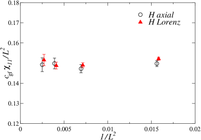
Figure 2: (Coulomb phase) Estimates of $c_{\rm gf}\chi_{11}/L^{2}$ versus $1/L^{2}$ in the hard Lorenz and hard axial gauge, where $c_{\rm gf}$ is a gauge-fixing dependent constant. We use $c_{\rm gf}=3$ for the Lorenz gauge fixing and $c_{\rm gf}=1$ for the axial one. Lorenz gauge data have been slightly shifted toward the right to improve readability. Results in the Coulomb phase, for $J=0.2$.

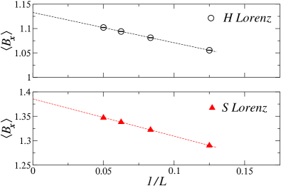
Figure 3: (Coulomb phase) Estimates of $\langle B_{\bm{x}}\rangle$ versus $1/L$ in the hard Lorenz (top) and soft Lorenz gauge with $\zeta=1$ (bottom). For $L\to\infty$ $\langle B_{\bm{x}}\rangle\approx 1.1328$ and $1.3857$ in the two cases, respectively. Results in the Coulomb phase, for $J=0.2$.

We start by investigating the behavior of the gauge model in the Coulomb phase (simulations for $J=0.2$). In the whole Coulomb phase the gauge field is expected to have long-range correlations, and thus $\chi_{\mu\nu}$ should diverge as $L$ increases, in all gauges considered. Results for the two hard gauges are reported in Fig. 2. We observe that $\chi_{\mu\nu}$ diverges as $L^{2}$ in both cases, a fact that is consistent with the analytic results for $J=0$ (in which case $1/L^{2}$ corrections are expected), see App. A. The relation Eq. (24) is fully confirmed by the data, see Fig. 2, and results in the soft gauges behave analogously and are in full agreement with relations (35) and (30).

Let us now consider the average of the photon mass operator $B_{\bm{x}}$. Results in the Lorenz gauges are reported in Fig. 3. In both case $\langle B_{\bm{x}}\rangle$ has a finite infinite-volume limit with corrections of order $1/L$. Again this is in agreement with the results for $J=0$ reported in App. A. We have determined the same quantity in the axial gauges obtaining a different result. In this case $\langle B_{\bm{x}}\rangle$ diverges with the system size as $L$ increases, see Fig. 4: $B_{\bm{x}}$ is not a well-defined operator in the infinite-volume limit. The different behavior can be understood by noting the completely different role the two gauge fixings play in infinite volume. In infinite volume, only the transformations $A_{{\bm{x}},\mu}^{\prime}=A_{{\bm{x}},\mu}+c_{\mu}$, where $c_{\mu}$ is a constant, leave the Lorenz gauge-fixed action invariant. Indeed, in the Lorenz gauge, a gauge transformation leaves $A_{{\bm{x}},\mu}$ invariant only if

$$\sum_{\mu}[\phi_{{\bm{x}}+\hat{\mu}}-2\phi_{\bm{x}}+\phi_{{\bm{x}}-\hat{\mu}}]=0$$ (37)

for all points ${\bm{x}}$. By working in Fourier space, one can show that all solutions of this equation can be written as $\phi_{\bm{x}}=a+\sum_{\mu}c_{\mu}x_{\mu}$, so that, $\Delta_{\mu}\phi_{\bm{x}}=c_{\mu}$. Note that these gauge transformations are valid only in infinite volume. In a finite volume with $C^{*}$ boundary conditions, the gauge fixing is complete and $c_{\mu}$ necessarily vanishes.

On the other hand, in the axial gauge, any gauge transformation with function $\phi_{\bm{x}}=\phi(x,y,z)$ that only depends on $x$ and $y$ leaves the action invariant. Thus, the axial-gauge action is invariant under a large set of space-dependent transformations and this causes the divergence of $\langle B_{\bm{x}}\rangle$. This result can also be understood by looking at the relation between the axial and Lorenz correlation functions, see Eq. (21). While the Lorenz correlation function is expected to be singular only for $p=0$ (due to the presence of the zero modes discussed above), the axial correlation function is singular for $p_{d}=0$, irrespective of the value of the other components of the momentum, i.e., on a $(d-1)$-dimensional momentum surface. These singularities make the sum appearing in Eq. (25) diverge as $L\to\infty$.

It is well known that perturbation theory in the axial gauges is problematic ZJ_book ; Leibbrandt:1987qv . The results presented here show that the difficulties one encounters using axial gauges are not simply technical ones due to the infrared problems of the perturbative expansion. Also nonperturbatively, axial gauges do not allow a proper definition of some gauge-dependent quantities, for instance, the photon-mass operator, in the infinite-volume limit.

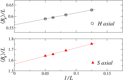
Figure 4: (Coulomb phase) Estimates of $\langle B_{\bm{x}}\rangle/L$ versus $1/L$ in the hard axial (top) and soft axial gauge with $\zeta=1$ (botton). For $L\to\infty$ $\langle B_{\bm{x}}\rangle/L\approx 0.5631$ and $1.563$ in the two cases, respectively. Results in the Coulomb phase, for $J=0.2$.

We have also determined the behavior of the susceptibility $\chi_{B}$, obtaining results that are analogous to those that hold for $J=0$. We find $\chi_{B}\sim L$ in Lorenz gauges and $\chi_{B}\sim L^{3}$ in axial gauges.

Finally, let us make a few comments on the apparently equivalent Lorenz gauge fixing

$$F_{L^{\prime},{\bm{x}}}(A)=\sum_{\mu=1}^{d}(A_{{\bm{x}}+\hat{\mu},\mu}-A_{{\bm{x}},\mu}),$$ (38)

which differs from the one reported in Eq. (10) in the choice of the lattice derivative (forward instead of backward). This gauge fixing function has several shortcomings. First of all, in even dimension, it does not represent a complete gauge fixing for some values of $L$. For instance, if $L=4n+2$ and $d=4$, transformations with [$\bm{x}=(x_{1},x_{2},x_{3},x_{4})$]

$$\phi_{\bm{x}}=A\cos\Bigl{[}{\pi\over 2}(x_{1}-x_{2})\Bigr{]}\cos\Bigl{[}{\pi\over 2}(x_{3}-x_{4})\Bigr{]}$$ (39)

leave $F_{L^{\prime},{\bm{x}}}(A)$ invariant and are consistent with the $C^{*}$ boundary conditions ($\phi_{\bm{x}}$ is antiperiodic). In $d=3$ the gauge fixing is complete in a finite volume. However, in infinite volume, $F_{L^{\prime},{\bm{x}}}(A)$ is invariant under a large set of gauge transformations, as it occurs in the axial case. Thus, we do not expect $B_{\bm{x}}$ to be a well-defined operator if $F_{L^{\prime},{\bm{x}}}(A)$ is used. For $J=0$, the average value of $B_{\bm{x}}$ diverges in the infinite-volume limit, see App. A. We have also performed some simulations for $J=0.2$, observing that also in this case $\langle B_{\bm{x}}\rangle$ increases as $L$ is varied.

IV.2 Higgs phase

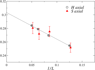
Figure 5: (Higgs phase) Estimates of $\chi_{11}$ (hard axial gauge) and $\chi_{11}-1$ (soft axial gauge with $\zeta=1$), versus $1/L$, in the Higgs phase, $J=0.4$. Soft axial gauge data have been slightly moved to the right to improve readability. The line is only meant to guide the eye, since we have no theoretical understanding of the possibile origin of the $1/L$ correction.

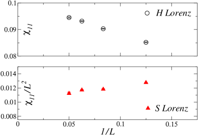
Figure 6: (Higgs phase) Top: Estimates of $\chi_{11}$ in the hard Lorenz gauge; bottom: Estimates of $\chi_{11}/L^{2}$ in the soft Lorenz gauge with $\zeta=1$. Results in the Higgs phase for $J=0.4$.

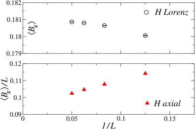
Figure 7: (Higgs phase) Top: Estimates of $\langle B_{\bm{x}}\rangle$ in the hard Lorenz gauge; bottom: Estimates of $\langle B_{\bm{x}}\rangle/L$ in the hard axial gauge. Results in the Higgs phase for $J=0.4$.

Let us now discuss the behavior of gauge-dependent observables in the Higgs phase (numerical simulations have been performed for $J=0.4$). In Fig. 5 we report the susceptibility $\chi_{11}$ for the hard and the soft axial gauge (with $\zeta=1$), versus $1/L$. In both cases $\chi_{11}$ has a finite limit as $L\to\infty$ and satisfies relation (30). The finite value in the Higgs phase is consistent with the presence of a finite photon mass. However, the apparent presence of size corrections that decay as $1/L$ points to an unusual behavior of the system, since in a standard massive phase corrections are typically expected to scale as $e^{-L/\xi}$.

In Fig. 6 we show results for the susceptibility $\chi_{11}$ in the Lorenz gauges. In the hard case, $\chi_{11}$ is finite in the infinite-volume limit and satisfies the exact relation (24) with the corresponding quantity in the hard axial gauge. Instead, in the soft Lorenz gauge, we find $\chi_{11}\sim L^{2}$. This divergence might be, erroneously, interpreted as an indication of the presence of physical long-range gauge correlations in the Higgs phase—this would be in contrast with the idea that the photon is massive. The correct interpretation is instead, that in the soft Lorenz gauge that are unphysical gauge modes that are long-ranged and contribute to $\chi_{\mu\nu}$, even though they do not have physical meaning. This interpretation is supported by Eq. (35) that we rewrite as

$$\chi_{11,L\zeta}=\chi_{11,HL}+{\zeta\over d^{2}\hat{p}_{\rm min}^{2}}\approx\chi_{11,HL}+{\zeta\over d^{2}\pi^{2}}L^{2}$$ (40)

where $\chi_{11,L\zeta}$ and $\chi_{11,HL}$ refer to the soft Lorenz gauge with parameter $\zeta$ and to the hard Lorenz gauge, respectively. Since $\chi_{11,HL}$ has a finite large-$L$ limit, this relation shows that the divergence of $\chi_{11,L\zeta}$ is only due to the last term, which has no physical meaning, and is related to the presence of propagating longitudinal modes that are instead completely suppressed in the hard gauge ($\zeta=0$).

Perturbation theory provides the recipe for the definition of a susceptibility that only couples the physical modes. We define

$$\widetilde{G}_{\rm tr}({\bm{p}})=\sum_{\mu\nu}\left(1-{\hat{p}_{\mu}\hat{p}_{\nu}\over\hat{p}^{2}}\right)\widetilde{G}_{\mu\nu}({\bm{p}}).$$ (41)

and a transverse susceptibility $\chi_{\rm tr}=\widetilde{G}_{\rm tr}({\bm{p}}_{a})$. Using the parametrization (22) we obtain

$$\chi_{\rm tr}=(d-1)(c_{L1}-c_{L2}).$$ (42)

Eq. (35) then implies

$$\chi_{\rm tr}(\zeta_{1})=\chi_{\rm tr}(\zeta_{2}).$$ (43)

The transverse susceptibility is independent of $\zeta$ and therefore is the same in hard and soft gauges. In particular, $\chi_{\rm tr}(\zeta)$ is finite in the Higgs phase for all values of $\zeta$, as expected.

The behavior of $\langle B_{\bm{x}}\rangle$ and of the corresponding susceptibility is analogous to that observed in the Coulomb phase, see Fig. 7. The average $\langle B_{\bm{x}}\rangle$ is well defined only for Lorenz gauges. In the axial gauge, we have instead $\langle B_{\bm{x}}\rangle\sim L$. This is not unexpected since the argument we have presented in the previous section, i.e., that the divergence of $\langle B_{\bm{x}}\rangle$ is related to the large number of quasi-zero modes present in the axial case, does not rely on any particular property of the two phases.

Finally, let us consider the susceptibility $\chi_{B}$. Not surprisingly, in the axial gauge data are consistent with a behavior $\chi_{B}\sim L^{3}$, as in the Coulomb phase. In the hard Lorenz case, we observe that $\chi_{B}$ is finite as $L$ increases. This is the expected behavior in the Higgs phase, in which the photon is massive. In the soft Lorenz gauge instead, data are consistent with $\chi_{B}\sim L$. It is easy to realize that this divergence is due to the contributions of the nonphysical longitudinal modes present for nonzero values of $\zeta$. The linear divergence with $L$ can be predicted by a simple argument. Let us assume that the hard-gauge correlation function has the form (at least for small values of $\bm{p}$)

$$\widetilde{G}_{\mu\nu}({\bm{p}},\zeta=0)={Z\over\hat{p}^{2}+M^{2}}\left(\delta_{\mu\nu}-{\hat{p}_{\mu}\hat{p}_{\nu}\over\hat{p}^{2}}\right),$$ (44)

and, as predicted by the Ward identities, that

$$\widetilde{G}_{\mu\nu}({\bm{p}},\zeta)=\widetilde{G}_{\mu\nu}({\bm{p}},\zeta=0)+\zeta{\hat{p}_{\mu}\hat{p}_{\nu}\over(\hat{p}^{2})^{2}}.$$ (45)

In a Gaussian approximation—we neglect irreducible four-field contributions—we have

$$\chi_{B}={2\over L^{d}}\sum_{\bm{p}}\sum_{\mu\nu}\widetilde{G}_{\mu\nu}({\bm{p}},\zeta)\widetilde{G}_{\mu\nu}(-{\bm{p}},\zeta),$$ (46)

and therefore,

$$\chi_{B} =2(d-1)Z^{2}{1\over L^{d}}\sum_{\bm{p}}{1\over(\hat{p}^{2}+M^{2})^{2}}+$$ (47)

$$+2\zeta{1\over L^{d}}\sum_{\bm{p}}{1\over(\hat{p}^{2})^{2}}.$$

The first sum has a finite limit as $L\to\infty$, while the second one, see App. A, diverges as $L$ and $\ln L$ in $d=3$ and $d=4$, respectively. Thus, in three dimensions the longitudinal modes give rise to a contribution that increases as $L$, in agreement with the numerical results. We conclude that the photon mass operator is not well-defined nonperturbatively in the Lorenz soft gauge, because of the contributions of the nonphysical longitudinal modes. Apparently, only the hard Lorenz gauge is a consistent gauge fixing in which the operator is correctly defined.

V Some field theory results

The results of the previous sections can be combined with QFT results to obtain some general predictions of the behavior of Abelian gauge systems at charged fixed points.

First, let us note that our previous results also allow us to predict that the anomalous dimension of the gauge field is the same in the axial gauge as in the Lorenz gauge. Indeed, as we have discussed before, the large-scale behavior of the susceptibilities $\chi_{\mu\nu}$ (for $\mu,\nu<d$) is the same for all gauge fixings (although some caution should be exercised in the soft Lorenz case). Indeed, a summary of the results obtained is the following:

1. the susceptibilities $\chi_{\mu\nu}$ ($\mu,\nu<d$) in the hard Lorenz and in the hard axial gauge differ only by a multiplicative constant: $2d/(d-1)$ for $\mu=\nu$ and $-d$ for $\mu\not=\nu$, see Eq. (24);

2. the susceptibilities in the hard and soft axial gauges differ by an additive constant, see Eq. (30);

3. the susceptibilities in the hard and soft Lorenz gauge behave differently, because of the coupling with the longitudinal modes. If one considers the transverse definition, see Eq. (41), results are independent of $\zeta$, i.e., are the same in the hard and soft case.

For the soft Lorenz gauge, one can prove to all orders of perturbation theory that HT96 ; ZJ_book $\eta_{A}=4-d$, independently of the nature of the matter fields. Indeed, the proof only relies on the relation $Z_{A}Z_{e}=1$ between the renormalization constants of the gauge field and of the electric charge $e$. This implies ZJ_book

$$\beta_{e^{2}}=\hat{e}_{r}^{2}(d-4+\eta_{A})\ ,$$ (48)

which connects the anomalous dimension $\eta_{A}$ of the gauge field, the $\beta$ function of the dimensionless charge $\hat{e}^{2}=e^{2}\mu^{d-4}$ ($\mu$ is the RG scale), and the renormalized dimensionless charge $\hat{e}_{r}$. At a transition which is associated with a charged fixed point, i.e., where the gauge theory provides the effective critical behavior, we have $\hat{e}_{r}^{2}\not=0$. Therefore, the fixed-point condition $\beta_{e^{2}}=0$ implies HT96

$$\eta_{A}=4-d.$$ (49)

Numerical results BPV-in-prep for the three-dimensional Abelian-Higgs model are in full agreement with this prediction.

A second interesting result concerns the parameter $\zeta$ that parametrizes the soft gauges. As a consequence of the Ward identities discussed in Sec. B, in the soft Lorenz gauge we have $\zeta=\zeta_{r}Z_{A}$, which implies

$$\beta_{\zeta}=-\zeta_{r}\eta_{A}.$$ (50)

The value $\zeta=0$ is a fixed point of this equation, as expected. Indeed, if we start from a model with a purely transverse gauge field, no longitudinal contributions are generated by the RG flow. Instead, if we start the flow from a value $\zeta\not=0$, $\zeta$ flows towards $+\infty$, indicating that the hard gauge fixing is an unstable fixed point, at least for $d<4$. Moreover, for $\zeta\not=0$ the large-scale behavior is singular, as the nongauge-invariant modes become unbounded under the RG transformations. Therefore, also QFT (which describes the critical behavior at charged transitions) predicts that only the hard Lorenz gauge fixing provides a consistent definition of nongauge-invariant quantities at the critical point in three dimensions.

Eqs. (49) and (50) allow us to predict the crossover behavior of $\chi_{\mu\nu}$ at a critical charged transition point in the soft Lorenz gauges. For $d<4$ we predict

$$\chi_{\mu\nu}(\alpha)=L^{2-\eta_{A}}f_{\mu\nu}(\zeta L^{\eta_{A}})=L^{d-2}f_{\mu\nu}(\zeta L^{4-d}).$$ (51)

This relation should hold for $L\to\infty$, $\zeta\to 0$ at fixed $\zeta L^{4-d}$. The function $f_{\mu\nu}(x)$ can be computed using Eq. (35). If $\chi_{\mu\nu}(\alpha=0)\approx a_{\mu\nu}L^{d-2}$ for $L\to\infty$, Eq. (35) implies

$$\chi_{\mu\nu}(\alpha) \approx a_{\mu\nu}L^{d-2}+{\zeta L^{2}\over d^{2}\pi^{2}}=$$ (52)

$$=L^{d-2}\left(a_{\mu\nu}+{1\over d^{2}\pi^{2}}\zeta L^{4-d}\right),$$

so that $f_{\mu\nu}(x)=a_{\mu\nu}+x/(d^{2}\pi^{2})$.

VI Conclusions

In this work we investigate the behavior of gauge correlations in Abelian gauge theories with noncompact gauge fields. Because of the unbounded nature of the fluctuations of the gauge fields, a rigorous definition of the model requires the introduction of a gauge fixing term. This is at variance with compact formulations (for instance, models with Wilson action), in which a gauge fixing is not required to make the model well defined. Here we consider two widely used gauge fixings, the axial and Lorenz one. We also distinguish between hard gauge fixings—in this case the partition function is given in Eq. (6)—and soft ones depending on a parameter $\zeta$—the corresponding partition function is given in Eq. (8).

Gauge-invariant correlations are obviously independent of the gauge-fixing procedure. On the other hand, the large-scale behavior of gauge-dependent quantities may have a nontrivial dependence. Here we first consider correlations of the gauge field $A_{{\bm{x}},\mu}$ and we derive general relations, independent of the nature of the matter couplings, between these correlations computed in the presence of different gauge fixings. Second, we consider the photon-mass composite operator $A_{{\bm{x}},\mu}^{2}$, which is usually introduced in the action, in perturbative calculations, as an infrared regulator of the theory.

As a specific example, we analyze the behavior of these correlation functions in the three-dimensional Abelian-Higgs model, in which an $N$-component complex scalar field is coupled with a noncompact real Abelian gauge field. In particular, we study their behavior in the so-called Coulomb and Higgs phases (see Fig. 1 for a sketch of the phase diagram). In the Coulomb phase, the correlation function $\widetilde{G}_{\mu\nu}({\bm{p}})$ of the gauge fields has the same small-momentum behavior as in the absence of matter fields, for all gauge fixings considered. In particular, the susceptibiity $\chi_{\mu\nu}$ defined in Eq. (16) diverges as $L^{2}$ in the infinite-volume limit. In the Higgs phase, we expect the photon to be massive and therefore $\chi_{\mu\nu}$ should be finite as $L\to\infty$. This turns out to be true for the axial soft and hard gauges and for the hard Lorenz gauge. On the other hand, $\chi_{\mu\nu}\sim L^{2}$ in the soft Lorenz gauge. This divergence is caused by the unphysical contributions due to the longitudinal modes that propagate in the soft Lorenz gauge.

While the behavior of $\widetilde{G}_{\mu\nu}({\bm{p}})$ in all gauges is consistent with the general picture that the photon is massless/massive in the Coulomb/Higgs phase, the interpretation of the results for the photon mass operator $B_{\bm{x}}=\sum_{\mu}A_{{\bm{x}},\mu}^{2}$ are more complicated. If we consider the soft and hard axial gauges, we find $\langle B_{\bm{x}}\rangle\sim L$ in both phases. The operator does not have a well-defined infinite-volume limit. The divergence is due to the presence of a $(d-1)$-dimensional family of quasi-zero modes, so that $A_{{\bm{x}},\mu}$ develops infinite-range fluctuations in the infinite-volume limit. Therefore, if an axial gauge fixing is used, $B_{\bm{x}}$ cannot be defined nonperturbatively. In the soft and hard Lorenz gauge, the average $\langle B_{\bm{x}}\rangle$ is finite as $L\to\infty$ in both phases, and thus the operator is well defined. However, in the Higgs phase, the susceptibility $\chi_{B}$ defined in Eq. (16) behaves differently in the hard and soft case. In the hard case, $\chi_{B}$ has a finite infinite-volume limit, as expected— the photon mass is finite. Instead, $\chi_{B}$ diverges as $L$ in the soft gauge. This divergence is due to the longitudinal modes that are not fully suppressed.

The results presented here show that neither the axial gauge nor the soft Lorenz gauge are appropriate for the study of generic gauge-dependent correlation functions. The first type of gauges suffers from the existence of an infinite family of quasi-zero modes, giving rise to spurious divergences, unrelated with the presence of long-range physical correlations. Soft Lorenz gauges suffer instead from the presence of propagating unphysical longitudinal modes, that, at least for $d<4$ and therefore in three dimensions, may hide the physical signal. Apparently, only the hard Lorenz gauge fixing provides a consistent model in which gauge-dependent correlations have the expected large-scale (small-momentum) behavior. It is interesting to observe that also QFT singles out the hard Lorenz gauge as the gauge of choice for the study of gauge correlations. Note that the shortcomings of the axial gauge and of the soft Lorenz gauge are not related to the nature of the matter fields but are due to intrinsic properties of the gauge fixings. Therefore, our conclusions should be relevant also for systems in which fermions are present.

Acknowledgement. Numerical simulations have been performed on the CSN4 cluster of the Scientific Computing Center at INFN-PISA.

Appendix A Critical behavior in the U(1) abelian gauge theory

In this Appendix we summarize the expressions of the observables defined in Sec. II for the free U(1) gauge theory, i.e., in the absence of matter fields. The susceptibilities $\chi_{\mu\nu}$ can be trivially derived from the small-momentum behavior of $\widetilde{G}_{\mu\nu}({\bm{p}})$, defined in Sec. II. Moreover, we have

$$\langle B_{\bm{x}}\rangle = {1\over V}\sum_{{\bm{p}}}\sum_{\mu\nu}\widetilde{G}_{\mu\nu}({\bm{p}}),$$ (53)

$$\chi_{B} = {2\over V}\sum_{{\bm{p}}}\sum_{\mu\nu}[\widetilde{G}_{\mu\nu}({\bm{p}})]^{2}\;.$$ (54)

Because of the $C^{*}$ boundary conditions the sums go over the momenta

$${\bm{p}}={\pi\over L}\left(2n_{1}+1,2n_{2}+1,2n_{3}+1\right),$$ (55)

with $0\leq n_{i}<L$.

A.1 Lorenz gauge

In the Lorenz gauge, the propagator $\widetilde{G}_{\mu\nu}({\bm{p}})$ is given by

$$\widetilde{G}_{\mu\nu}({\bm{p}})={1\over\kappa}{\delta_{\mu\nu}\over\hat{p}^{2}}+{\zeta\kappa-1\over\kappa}{\hat{p}_{\mu}\hat{p}_{\nu}\over(\hat{p}^{2})^{2}},$$ (56)

where $\hat{p}_{\mu}=2\sin p_{\mu}/2$ and $\hat{p}^{2}=\sum_{\mu}\hat{p}_{\mu}^{2}$. It follows that

$$\chi_{\mu\nu} =(d\delta_{\mu\nu}+\zeta\kappa-1){1\over\kappa d^{2}\hat{p}_{\rm min}^{2}}\ ,$$ (57)

$$\langle B_{\bm{x}}\rangle ={d-1+\zeta\kappa\over\kappa}I_{d,1}(L)\ ,$$

$$\chi_{B} ={2(d-1+\zeta^{2}\kappa^{2})\over\kappa^{2}}I_{d,2}(L)\ ,$$

where $p_{\rm min}=\pi/L$ and

$$I_{d,n}(L)={1\over L^{d}}\sum_{\bm{p}}{1\over(\hat{p}^{2})^{n}}.$$ (58)

The behavior of the sums $I_{d,n}$ depends on the dimension $d$. For $d>2$, $I_{d,1}$ has a finite limit for $L\to\infty$, while it diverges logarithmically in $d=2$. In particular, in $d=3$ we have GZ-77 ; JZ-01

$$I_{3,1}(L)\approx\int_{[-\pi,\pi]^{3}}{d^{3}p\over(2\pi)^{3}}{1\over\hat{p}}=$$ (59)

$$={1\over 192\pi^{3}}(\sqrt{3}-1)\Gamma\left({1\over 24}\right)^{2}\Gamma\left({11\over 24}\right)^{2}\approx$$

$$\approx 0.252731\ .$$

Instead, the sum $I_{d,2}$ diverges for $L\to\infty$ in dimension $d\leq 4$, as $L^{4-d}$ (as $\ln L$ in $d=4$). We find

$$I_{3,2}(L)\approx a_{2}L[1+O(L^{-1})] a_{2}\approx 0.015216\;,$$ (60)

$$I_{4,2}(L)\approx a_{2}\ln L+O(1) a_{2}\approx{1\over 8\pi^{2}}\;.$$

Thus, in three dimensions the susceptibilities $\chi_{\mu\nu}$ and $\chi_{B}$ diverge as $L^{2}$ and $L$, respectively, while $\langle B_{\bm{x}}\rangle$ is finite.

A.2 Axial gauge

In the axial gauge

$$\widetilde{G}_{\mu\nu}({\bm{p}}) = {1\over\kappa}{\delta_{\mu\nu}\over\hat{p}^{2}}+{\hat{p}_{\mu}\hat{p}_{\nu}\over\hat{p}_{d}^{2}}\left({1\over\kappa\hat{p}^{2}}+\zeta\right),$$ (61)

if both $\mu$ and $\nu$ are not equal to $d$. Otherwise, we have

$$\widetilde{G}_{\mu\nu}({\bm{p}}) = \zeta{\hat{p}_{\mu}\hat{p}_{\nu}\over\hat{p}_{d}^{2}}.$$ (62)

As for the susceptibilities, we find $\chi_{d\mu}=\zeta$ and, for $\mu,\nu<d$,

$$\chi_{\mu\nu}{\delta_{\mu\nu}+1\over d\kappa}{1\over\hat{p}_{\rm min}^{2}}+\zeta\approx{\delta_{\mu\nu}+1\over d\kappa\pi^{2}}L^{2},$$ (63)

where $p_{\rm min}=\pi/L$. As expected, $\chi_{d\mu}$ is finite (it vanishes in the hard axial gauge for which $\zeta=0$), while the other susceptibility components diverge as $L^{2}$. Although the large-$L$ behavior is the same as in the Lorenz case, here the asymptotic behavior is $\zeta$ independent: the susceptibilities behave identically in the hard and soft axial case, a result that does not hold in the Lorenz case.

As for $\langle B_{\bm{x}}\rangle$ and $\chi_{B}$ we find

$$\langle B_{\bm{x}}\rangle={1\over\kappa}((d-2)I_{d,1}+J_{1})+\zeta(1+(d-1)J_{1}J_{-1}),$$ (64)

$$\chi_{B}=2\zeta^{2}+$$

$$+2\zeta^{2}(d-1)(2J_{1}J_{-1}+(d-2)J_{2}J_{-1}^{2}+J_{2}J_{-2})$$

$$+{2\over\kappa^{2}}((d-2)I_{d,2}+J_{2}+2(d-1)\zeta\kappa J_{2}J_{-1}),$$

where the quantities $J_{n}(L)$ correspond to the one-dimensional sums ($p=(2n+1)\pi/L$ with $n=0,\dots,L-1$)

$$J_{n}(L)={1\over L}\sum_{p}\hat{p}^{-2n}.$$ (65)

Since we have (these expressions can be derived as in App. B.1.d of Ref. CP-98 )

$$J_{2} ={1\over 48}L(L^{2}+2),$$ (66)

$$J_{1} ={L\over 4},$$

$$J_{-1} =2,$$

$$J_{-2} =6,$$

we obtain for large values of $L$ for $d>2$:

$$\langle B_{\bm{x}}\rangle \approx{1+2(d-1)\zeta\kappa\over 4\kappa}L,$$ (67)

$$\chi_{B} \approx{1\over 24\kappa^{2}}[1+4(d-1)\zeta\kappa+$$

$$\quad+2(d-1)(2d-1)\zeta^{2}\kappa^{2}]L^{3}.$$

Note that $\langle B_{\bm{x}}\rangle$ diverges, at variance with what happens in the Lorenz case. From a technical point of view this is due to the fact that the axial-gauge propagator is more divergent than the Lorenz one: indeed, in the axial gauge $\widetilde{G}_{\mu\nu}({\bm{p}})$ diverges as $p_{d}\to 0$, for any value of the other momentum components, while in the Lorenz gauge a divergence is only observed as $|{\bm{p}}|\to 0$. More intuitively, note that, in infinite volume, the axial-gauge fixed Hamiltonian is still invariant under the gauge transformations (3) if the function $\phi_{\bm{x}}=\phi_{(x_{1},\ldots,x_{d})}$ depends on $x_{i}$ with $i<d$ only. This should be compared with the Lorenz case, in which only gauge transformations with $\Delta_{\mu}\phi_{\bm{x}}=c_{\mu}$, where $c_{\mu}$ is $x$-independent, leave the infinite-volume gauge-fixed Hamiltonian invariant. The presence of this large family of quasi-zero modes is responsible for the divergence of the variance of $A_{{\bm{x}},\mu}$ for $\mu<d$.

A.3 Some other gauge fixings

It is interesting to note that the results for the Lorenz gauge apply only to the discretization (10). If instead the discretization (38) is used, different results are obtained. Indeed, in the latter case, in the infinite-volume limit, the gauge-fixed Hamiltonian is invariant under a large family of gauge transformations. For instance, one can consider transformations like those reported in Eq. (39). To determine the full set of transformations that leave $F_{L^{\prime},\bm{x}}(A)$ invariant in infinite volume, we work in Fourier space and consider a function $\phi_{\bm{x}}$ of the form

$$\phi_{{\bm{x}}}=ae^{i{\bm{p}}\cdot{\bm{x}}}+\bar{a}e^{-i{\bm{p}}\cdot{\bm{x}}},$$ (68)

where $a$ is an arbitrary complex constant. These transformations leave $F_{L^{\prime},\bm{x}}(A)$ invariant, if at least one of these two conditions is satisfied:

$$\sum_{\mu}\cos p_{\mu}(1-\cos p_{\mu})=0,$$ (69)

$$\sum_{\mu}\sin p_{\mu}(1-\cos p_{\mu})=0.$$

If only the first (the second) equation is satisfied, then $a$ is necessarily real (purely imaginary). The transformation (39) corresponds to taking ${\bm{p}}=(\pi/2,-\pi/2,\pi/2,-\pi/2)$ and a real constant $a$. We have studied numerically the equations (69) in three dimensions, finding that both equations are satisfied on a two-dimensional surface in momentum space. The presence of this family of gauge transformations that leave the Hamiltonian invariant, implies that the correlation function $\widetilde{G}_{\mu\nu}(\bm{p})$ is singular in ${\bm{p}}$ space. In turn, this implies (we have performed a numerical check) the divergence of the variance of $A_{\bm{x}}$, as it also occurs in the axial gauge.

Finally, we would like to make some comments on the Coulomb gauge that we can define as

$$F_{L,{\bm{x}}}(A)=\sum_{\mu=1}^{d-1}(A_{{\bm{x}},\mu}-A_{{\bm{x}}-\hat{\mu},\mu}).$$ (70)

In the hard case $\zeta=0$, the correlation function is given by

$$\widetilde{G}_{\mu\nu}({\bm{p}}) = {1\over\kappa}{\delta_{\mu\nu}\over\hat{p}^{2}}-{1\over\kappa}{p_{\mu}p_{\nu}\over\hat{p}^{2}\hat{p}_{T}^{2}}\qquad\mu,\nu<d$$

$$\widetilde{G}_{d\mu} = 0\hphantom{xxxxxxxxxxxxxxxx}\mu<d$$

$$\widetilde{G}_{dd} = {1\over\kappa}{1\over\hat{p}_{T}^{2}}$$ (71)

where $\hat{p}_{T}^{2}=\sum_{\mu=1}^{d-1}\hat{p}_{\mu}^{2}$. The susceptibilities diverge as $L^{2}$ while $\langle B_{\bm{x}}\rangle$ is given by

$$\langle B_{\bm{x}}\rangle={1\over\kappa}(2I_{d,1}+I_{d-1,1}).$$ (72)

In four dimensions, both sums are finite, therefore $\langle B_{\bm{x}}\rangle$ is well defined. In three dimensions, however, the result depends on the two-dimensional sum $I_{2,1}$, which diverges logarithmically. Therefore, for $d=3$, the photon mass operator is not well-defined in the Coulomb gauge.

Appendix B Ward identities in different gauges

A crucial ingredient in the derivations presented in Sec. III are the Ward identities satisfied by the correlation functions. We derive them here for the generic gauge-fixing function introduced in Sec. III, see Eq. (5). The corresponding function $S_{\rm GF}(A)$, defined in Eq. (7) is given by

$$S_{M}(A) =\frac{1}{2\zeta V}\sum_{{\bm{p}}\,\alpha\beta}M_{\alpha}({\bm{p}})M_{\beta}(-{\bm{p}})e^{-i(p_{\alpha}-p_{\beta})/2}\times$$ (73)

$$\qquad\qquad\times\widetilde{A}_{\alpha}({\bm{p}})\widetilde{A}_{\beta}(-{\bm{p}}).$$

Under an infinitesimal gauge transformation, we have

$$\delta S_{M}={1\over V}\sum_{\bm{p}}\delta_{M}({\bm{p}})\widetilde{\phi}({\bm{p}}),$$ (74)

$$\delta_{M}({\bm{p}})={1\over\zeta}\sum_{\alpha\beta}M_{\alpha}({\bm{p}})M_{\beta}(-{\bm{p}})e^{-i(p_{\alpha}-p_{\beta})/2}\times$$

$$\qquad\qquad\times(i\hat{p}_{\alpha})\widetilde{A}_{\beta}(-{\bm{p}}).$$

If we now consider $\langle A_{{\bm{x}},\gamma}\rangle$ and require its invariance under changes of variable represented by infinitesimal gauge transformations, we obtain

$$\langle\Delta_{\gamma}\phi_{\bm{x}}+A_{{\bm{x}},\gamma}\delta S_{M}\rangle=0.$$ (75)

In Fourier space, this implies the relation

$${1\over\zeta}\sum_{\alpha\beta}M_{\alpha}({\bm{p}})M_{\beta}(-{\bm{p}})e^{-i(p_{\alpha}-p_{\beta})/2}\hat{p}_{\alpha}\widetilde{G}_{\gamma\beta}({\bm{p}})=\hat{p}_{\gamma}.$$ (76)

In the axial gauge we have $M_{\alpha}({\bm{p}})=\delta_{\alpha d}$, while in the Lorenz gauge we have $M_{\alpha}({\bm{p}})=-e^{ip_{\alpha}/2}i\hat{p}_{\alpha}$. Substituting these relations in Eq. (76), we obtain Eqs. (28) and (33).

References

- (1) I. Montvay and G. Münster, Quantum Fields on a Lattice, (Cambridge University Press, 1994).
- (2) T. DeGrand and C. DeTar, Lattice methods for Quantum Chromodynamics (World Scientific, 2006)
- (3) J. Zinn-Justin, Quantum Field Theory and Critical Phenomena (Clarendon Press, 2002)
- (4) A. Pelissetto and E. Vicari, Critical phenomena and renormalization group theory, Phys. Rept. 368, 549 (2002)
- (5) S. Sachdev, Quantum Phase Transitions (Cambridge University Press, 2011).
- (6) E. Seiler, Gauge theories as a problem of constructive quantum field theory and statistical mechanics Lect. Notes Phys. 159 (Springer-Verlag, 1982).
- (7) J. Glimm and A. Jaffe, Quantum Physics (Springer-Verlag, 1987)
- (8) D. J. Gross and F. Wilczek, Ultraviolet Behavior of Nonabelian Gauge Theories, Phys. Rev. Lett. 30, 1343 (1973).
- (9) H. D. Politzer, Reliable Perturbative Results for Strong Interactions?, Phys. Rev. Lett. 30, 1346 (1973).
- (10) S. R. Coleman and D. J. Gross, Price of asymptotic freedom, Phys. Rev. Lett. 31, 851 (1973).
- (11) M. Moshe and J. Zinn-Justin, Quantum field theory in the large limit: A review, Phys. Rep. 385, 69 (2003).
- (12) K. G. Wilson and J. B. Kogut, The Renormalization group and the epsilon expansion, Phys. Rept. 12, 75 (1974).
- (13) G. Bhanot and M. Creutz, The Phase Diagram of and (1) Gauge Theories in Three-dimensions, Phys. Rev. D 21, 2892 (1980)
- (14) M. Caselle, M. Panero, R. Pellegrini, and D. Vadacchino, A different kind of string, J. High Ener. Phys. 01, 105 (2015).
- (15) A. Athenodorou and M. Teper, On the spectrum and string tension of U(1) lattice gauge theory in 2 + 1 dimensions, J. High Ener. Phys. 01, 063 (2019).
- (16) M. J. Teper, SU(N) gauge theories in (2+1)-dimensions, Phys. Rev. D 59, 014512 (1999).
- (17) A. Athenodorou and M. Teper, SU(N) gauge theories in 2+1 dimensions: glueball spectra and k-string tensions, J. High. Ener. Phys. 02, 015 (2017).
- (18) C. Bonati and S. Morlacchi, Flux tubes and string breaking in three dimensional SU(2) Yang-Mills theory, Phys. Rev. D 101, 094506 (2020).
- (19) T. Senthil, L. Balents, S. Sachdev, A. Vishwanath and M. P. A. Fisher, Quantum Criticality beyond the Landau-Ginzburg-Wilson Paradigm, Phys. Rev. B 70, 144407 (2004).
- (20) E. Fradkin, Field Theories of Condensed Matter Physics (Cambridge University Press, 2013).
- (21) S. Sachdev, Topological order, emergent gauge fields, and Fermi surface reconstruction, Rept. Prog. Phys. 82, 014001 (2019).
- (22) R. Moessner, J. E. Moore, Topological Phases of Matter (Cambridge University Press, 2021).
- (23) B. I. Halperin, T. C. Lubensky, and S. K. Ma, First-Order Phase Transitions in Superconductors and Smectic-A Liquid Crystals, Phys. Rev. Lett. 32, 292 (1974).
- (24) R. Folk and Y. Holovatch, On the critical fluctuations in superconductors, J. Phys. A 29, 3409 (1996).
- (25) B. Ihrig, N. Zerf, P. Marquard, I. F. Herbut, and M. M. Scherer, Abelian Higgs model at four loops, fixed-point collision and deconfined criticality, Phys. Rev. B 100, 134507 (2019).
- (26) A. Das, Phase transition in gauge theory with many fundamental bosons, Phys. Rev. B 97, 214429 (2018).
- (27) S. Sachdev, H. D. Scammell, M. S. Scheurer and G. Tarnopolsky, Gauge theory for the cuprates near optimal doping, Phys. Rev. B 99, 054516 (2019).
- (28) C. Bonati, A. Franchi, A. Pelissetto and E. Vicari, Three-dimensional lattice SU() gauge theories with multiflavor scalar fields in the adjoint representation, Phys. Rev. B 104, 115166 (2021).
- (29) C. Bonati, A. Franchi, A. Pelissetto and E. Vicari, Phase diagram and Higgs phases of three-dimensional lattice SU() gauge theories with multiparameter scalar potentials, Phys. Rev. E 104, 064111 (2021).
- (30) J. Braun, H. Gies, L. Janssen, and D. Roscher, Phase structure of many-flavor QED3, Phys. Rev. D 90, 036002 (2014).
- (31) I. F. Herbut, Chiral symmetry breaking in three-dimensional quantum electrodynamics as fixed point annihilation, Phys. Rev. D 94, 025036 (2016).
- (32) B. Ihrig, L. Janssen, L. N. Mihaila, and M. M. Scherer, Deconfined criticality from the QED3-Gross-Neveu model at three loops, Phys. Rev. B 98, 115163 (2018).
- (33) J. A. Gracey, Fermion bilinear operator critical exponents at in the QED-Gross-Neveu universality class, Phys. Rev. D 98, 085012 (2018).
- (34) C. Bonati, A. Pelissetto and E. Vicari, Lattice Abelian-Higgs model with noncompact gauge fields, Phys. Rev. B 103, 085104 (2021).
- (35) C. Bonati and N. Francini, Noncompact lattice Higgs model with Abelian discrete gauge groups: Phase diagram and gauge symmetry enlargement, Phys. Rev. B 107, 035106 (2023).
- (36) C. Bonati, A. Pelissetto and E. Vicari, Higher-charge three-dimensional compact lattice Abelian-Higgs models, Phys. Rev. E 102, 062151 (2020).
- (37) C. Bonati, A. Pelissetto and E. Vicari, Critical behaviors of lattice U(1) gauge models and three-dimensional Abelian-Higgs gauge field theory, Phys. Rev. B 105, 085112 (2022)
- (38) A. Pelissetto and E. Vicari, Three-dimensional ferromagnetic CP(N-1) models, Phys. Rev. E 100, 022122 (2019).
- (39) A. Pelissetto and E. Vicari, Large- behavior of three-dimensional lattice CPN-1 models, J. Stat. Mech. 2003, 033209 (2020).
- (40) A. Pelissetto and E. Vicari, Multicomponent compact Abelian-Higgs lattice models, Phys. Rev. E 100, 042134 (2019).
- (41) G. Bracci-Testasecca and A. Pelissetto, Multicomponent gauge-Higgs models with discrete Abelian gauge groups, J. Stat. Mech.: Th. Expt. 043101 (2023).
- (42) O. I. Motrunich and A. Vishwanath, Comparative study of Higgs transition in one-component and two-component lattice superconductor models, [arXiv:0805.1494 [cond-mat.stat-mech]] (unpublished).
- (43) A. B. Kuklov, M. Matsumoto, N. V. Prokof’ev, B. V. Svistunov, and M. Troyer, Deconfined Criticality: Generic First-Order Transition in the SU(2) Symmetry Case, Phys. Rev. Lett. 101, 050405 (2008) [arXiv:0805.4334 [cond-mat.stat-mech]].
- (44) O. I. Motrunich and A. Vishwanath, Emergent photons and transitions in the O(3) -model with hedgehog suppression, Phys. Rev. B 10, 075104 (2004).
- (45) G. Murthy and S. Sachdev, Actions of hedgehogs instantons in the disordered phase of 2+1 dimensional CPN-1 model, Nucl. Phys. B 344, 557 (1990).
- (46) G. J. Sreejith and S. Powell, Scaling dimensions of higher-charge monopoles at deconfined critical points, Phys. Rev. B 92, 184413 (2015).
- (47) A. Pelissetto and E. Vicari, Three-dimensional monopole-free models, Phys. Rev. E 101, 062136 (2020).
- (48) C. Bonati, A. Pelissetto and E. Vicari, Three-dimensional monopole-free CPN-1 models: behavior in the presence of a quartic potential, J. Stat. Mech. 2206, 063206 (2022).
- (49) C. Bonati, A. Pelissetto, and E. Vicari, in preparation.
- (50) S. Elitzur, Impossibility of Spontaneously Breaking Local Symmetries, Phys. Rev. D 12, 3978 (1975).
- (51) G. F. De Angelis, D. de Falco and F. Guerra, A Note on the Abelian Higgs-Kibble Model on a Lattice: Absence of Spontaneous Magnetization, Phys. Rev. D 17, 1624 (1978).
- (52) C. Itzykson and J. M. Drouffe, Statistical field theory. vol. 1: from Brownian motion to renormalization and lattice gauge theory, (Cambridge University Press, 1989).
- (53) A. S. Kronfeld and U. J. Wiese, SU(N) gauge theories with C periodic boundary conditions. 1. Topological structure, Nucl. Phys. B 357, 521 (1991).
- (54) B. Lucini, A. Patella, A. Ramos and N. Tantalo, Charged hadrons in local finite-volume QED+QCD with C∗ boundary conditions, JHEP 02, 076 (2016).
- (55) H. J. Rothe Lattice gauge theories. An introduction (World Scientific, 2005).
- (56) C. Bonati, A. Pelissetto and E. Vicari, Breaking of Gauge Symmetry in Lattice Gauge Theories, Phys. Rev. Lett. 127, 091601 (2021)
- (57) G. Leibbrandt, Introduction to Noncovariant Gauges, Rev. Mod. Phys. 59, 1067 (1987)
- (58) I. F. Herbut and Z. Tešanović Critical Fluctuations in Superconductors and the Magnetic Field Penetration Depth, Phys. Rev. Lett. 76, 4588 (1996).
- (59) M. L. Glasser and I. J. Zucker, Extended Watson integrals for the cubic lattices, Proc. Natl. Acad. Sci. USA 74, 1800 (1977).
- (60) G. S. Joyce and I. J. Zucker, Evaluation of the Watson integral and associated logarithmic integral for the -dimensional hypercubic lattice, J. Phys. A: Math. Gen. 34, 7349 (2001).
- (61) S. Caracciolo and A. Pelissetto, Corrections to Finite-Size Scaling in the Lattice -Vector Model for , Phys. Rev. D 58,105007 (1998).