Hydra II: Characterisation of Aegean, Caesar, ProFound, PyBDSF, and Selavy source finders.

Abstract

We present a comparison between the performance of a selection of source finders using a new software tool called Hydra. The companion paper, Paper I, introduced the Hydra tool and demonstrated its performance using simulated data. Here we apply Hydra to assess the performance of different source finders by analysing real observational data taken from the Evolutionary Map of the Universe (EMU) Pilot Survey. EMU is a wide-field radio continuum survey whose primary goal is to make a deep ($20\mu$Jy/beam RMS noise), intermediate angular resolution ($15^{\prime\prime}$), 1 GHz survey of the entire sky south of $+30^{\circ}$ declination, and expecting to detect and catalogue up to 40 million sources. With the main EMU survey expected to begin in 2022 it is highly desirable to understand the performance of radio image source finder software and to identify an approach that optimises source detection capabilities. Hydra has been developed to refine this process, as well as to deliver a range of metrics and source finding data products from multiple source finders. We present the performance of the five source finders tested here in terms of their completeness and reliability statistics, their flux density and source size measurements, and an exploration of case studies to highlight finder-specific limitations.

1 Introduction

We are entering a new era of radio surveys, digging ever deeper and with greater sky coverage, providing catalogues with tens of millions of sources (Norris, 2017), with increasing data rates, up to hundreds of gigabytes per second (Whiting & Humphreys, 2012). This has created a need for source finder (SF) software tools that are up to the challenge (as discussed in Paper I). The motivation to assess the performance of and to characterise such tools has led to a number of data challenges in recent years (e.g., Hopkins et al., 2015; Bonaldi et al., 2021).

As a consequence, so-called NxGen SFs, capable of efficiently handling large image tiles through multiprocessing (see Paper I) have been developed, and include Aegean (Hancock et al., 2012, 2018) and Selavy (Whiting & Humphreys, 2012), for handling compact or marginally extended sources, and Caesar (Compact And Extended Source Automated Recognition, Riggi et al., 2016, 2021), for handling compact and extended sources with diffuse emission. SFs developed initially for use with optical images have also been explored to understand their performance on radio image data. These include CuTex (Curvature Threshold Extractor, Molinari et al., 2010) for its ability to extract compact sources in the presence of intense background fluctuations, SExtractor (Source Extractor, Bertin & Arnouts, 1996) for its ability to handle extended sources, and ProFound (Robotham et al., 2018; Hale et al., 2019; Boyce, 2020) for its ability to handle extended sources with diffuse emission. Traditional Gaussian fitting SFs, capable of handling compact sources, such as APEX (Astronomical Point source Extractor, Makovoz & Marleau, 2005), PyBDSF (Python Blob Detector and Source Finder, Mohan & Rafferty, 2015), and SAD (Search and Destroy, Condon et al., 1998), have also been tested in such challenges. These SFs are just the tip of the iceberg, with new tools and approaches continuing to be explored (e.g., Hopkins et al., 2015; Wu et al., 2018; Lukic et al., 2019; Sadr et al., 2019; Koribalski et al., 2020; Bonaldi et al., 2021; Magro et al., 2022). This wide variety of tools and techniques makes comparison studies challenging, as it requires expertise spanning an extensive set of quite diverse SF tools, and hence often requires large collaborative efforts (e.g., Hopkins et al., 2015; Bonaldi et al., 2021). We have developed a new software tool, Hydra (see Paper I), to ease this effort.

Hydra is an extensible multi-SF comparison and cataloguing tool, requiring minimal expert knowledge of the underlying SFs from the user. Hydra is extensible, with the scope for adding new SFs in a modular fashion, using containerisation. Hydra currently incorporates Aegean, Caesar, ProFound, PyBDSF, and Selavy.

Hydra is designed for SFs with RMS and island-like parameters, which are optimised by reducing the False Detection Rate (FDR, Whiting, 2012) through a Percentage Real Detections (PRD, e.g., Williams et al., 2016; Hale et al., 2019) metric (we use a 90% PRD cutoff, see Paper I). It also provides optional RMS box parameter pre-optimisation, using bane (Hancock et al., 2012) in a process to minimize the background noise (referred to as $\mu$–optimisation, see Paper I). Hydra is designed to handle simulated images with injected ($\mathcal{J}$) sources, and real (i.e., deep or $\mathcal{D}$) images through comparison of detections in shallow ($\mathcal{S}$) images (i.e., images with $5\sigma$ noise added), for which detections in the $\mathcal{D}$-images are assumed as real. This leads to a rich set of statistics, including completeness ($\mathcal{C}$) and reliability ($\mathcal{R}$) metrics. We define $\mathcal{C}$ as the ratio of SF detections to real sources, and $\mathcal{R}$ as the ratio of SF detections that are real to detected sources. In our terminology, for $\mathcal{D}$ or $\mathcal{S}$ images with known input sources $\mathcal{J}$, these are $\mathcal{C_{D}}$ and $\mathcal{R_{D}}$, or $\mathcal{C_{S}}$ and $\mathcal{R_{S}}$, respectively. For real images, we use $\mathcal{C_{DS}}$ and $\mathcal{R_{DS}}$ describing sources detected in an $\mathcal{S}$ image with respect to sources in $\mathcal{D}$ assumed to be real. For formal definitions see Paper I.

A match is defined as the overlap between source components (components or sources, interchangeably, herein), which is achieved through a clustering technique (see Paper I). The technique is also used to associate SF components, from all SF $\mathcal{D}$ and $\mathcal{S}$ catalogues (including $\mathcal{J}$), spatially together into clumps.

Hydra produces a cluster catalogue with sets of rows marked by clump ID (clump_id), defining image depths ($\mathcal{D,\,S}$), spatial positioning, component sizes, flux densities, etc., with links to SF $\mathcal{D}$ and $\mathcal{S}$ (including $\mathcal{J}$) catalogues. It also includes a match ID (match_id), indicating the closest $\mathcal{D}$ and $\mathcal{S}$ associations. This catalogue is used to create a rich set of diagnostic plots and and cutouts of annotated and unannotated images and residual images, which can be accessed through a local web-browser based Hydra Viewer tool (Paper I). The user can also mine Hydra’s database to produce other diagnostics.

This paper is part two of a two part series. In Paper I, we introduced the Hydra software suite and evaluated the tool using $2^{\circ}\times 2^{\circ}$ simulated-compact (CMP) and simulated-extended (EXT) images. In this paper, a comparison study of Aegean, Caesar, ProFound, PyBDSF, and Selavy is performed using a real $2^{\circ}\times 2^{\circ}$ EMU pilot survey (Norris et al., 2021) image sample, along with the previous simulated data. We precede this with a brief overview of relevant radio surveys.

2 Radio Surveys

Over the last two decades radio surveys have progressed in depth ($\sigma_{rms}$), resolution ($\delta\theta_{res.}$), and sky coverage, due to technological advancements. At the Karl G. Jansky Very Large Array (JVLA, or VLA) in New Mexico, the ongoing VLA Sky Survey (VLASS, Lacy et al., 2020; Gordon et al., 2020, 2021) has better angular resolution and sensitivity than its predecessors, the National Radio Astronomy Observatory (NRAO) VLA Sky Survey (NVSS, Condon et al., 1998) and the Faint Images of the Radio Sky at Twenty-cm survey (FIRST, Becker et al., 1995; Helfand et al., 2015). Other surveys with Northern hemisphere telescopes include the Tata Institute of Fundamental Research (TIFR) Giant Metrewave Radio Telescope (GMRT) Sky Survey – Alternative Data Release (TGSS–ADR, Intema et al., 2017) at the GMRT (Khodad India), the Low-Frequency Array (LOFAR) Two-metre Sky Survey (LoTSS, Shimwell et al., 2017, 2019, 2022) at the LOFAR network (spanning Europe, Röttgering, 2003; van Haarlem et al., 2013) survey, the Westerbork Observations of the Deep APERture Tile In Focus (APERTIF) Northern-Sky (WODAN, Röttgering, 2010; Riggi et al., 2016) at the Westerbork Synthesis Radio Telescope (WSRT; Netherlands, Oosterloo et al., 2009; Apertif, 2016), and the Allen Telescope Array (ATA) Transients Survey (ATATS, Croft et al., 2011) at the ATA (California). The upper partition of Table 1 summarises the characteristics of these surveys.

Table 1: Radio surveys in the Northern (upper partition) and Southern (lower partition) hemispheres, with columns indicating the telescope (Telescope), radio survey (Survey), percentage sky-coverage (Sky), resolution ($\delta\theta_{res.}$), frequency ($\nu$), and depth ($\sigma_{rms}$).

Telescope	Survey	Sky	$\delta\theta_{res.}$	$\nu$	$\sigma_{rms}$
					$\left(\!\frac{\mu\mbox{Jy}}{\mbox{beam}}\!\right)$
VLA	NVSS	82%	$45^{\prime\prime}$	1.4 GHz	450
	FIRST	25%	$5.4^{\prime\prime}$	1.4 GHz	130
	VLASS	82%	$2.5^{\prime\prime}$	3.0 GHz	70
GMRT	TGSS-ADR	90%	$25^{\prime\prime}$	150 MHz	5
LOFAR	LoTSS	50%	$6^{\prime\prime}$	144 MHz	70
WSRT	WODAN	1%	$15^{\prime\prime}$	1.3 GHz	10
ATA	ATATS	1.7%	$150^{\prime\prime}$	1.4 GHz	150
ASKAP	EMU	75%	$14^{\prime\prime}$	940 MHz	15
	WALLABY	75%	$30^{\prime\prime}$	1.4 GHz	1 600
	VAST	1.8–24%	$10^{\prime\prime}$	1.1–1.4 GHz	10–500
	RACS	83%	$15^{\prime\prime}$	890 MHz	250
MWA	GLEAM	60%	$2^{\prime}\;$	200 MHz	50 000
MeerKAT	MIGHTEE	0.05%	$6^{\prime\prime}$	0.9–1.7 GHz	1
SKAMP	SUMSS	25%	$45^{\prime\prime}$	840 MHz	8
	MGPS-2	25%	$2^{\prime\prime}$	840 MHz	8
ATCA	SCORPIO	0.0097%	$10^{\prime\prime}$	2.1 GHz	30
	ATLAS	0.0090%	$6^{\prime\prime}$	1.4 GHz	10

Surveys with Southern hemisphere telescopes include those with ASKAP (Johnston et al., 2007, 2008), at the Murchison Radio Observatory (MRO) in Australia, such as EMU (Norris et al., 2011, 2021), Widefield ASKAP L-band Legacy All-sky Blind surveY (WALLABY, Koribalski et al., 2020), Variables and Slow Transients (VAST, Banyer et al., 2012; Murphy et al., 2013, 2021), and Rapid ASKAP Continuum Survey (RACS, McConnell et al., 2020; Hale et al., 2021). MRO is also home to the Murchison Widefield Array (MWA, Lonsdale et al., 2009; Tingay et al., 2013; Wayth et al., 2015) which conducted the GaLactic and Extragalactic All-Sky MWA (GLEAM, Wayth et al., 2015; Hurley-Walker et al., 2017) survey. These facilities along with the Hydrogen Epoch of Reionisation Array (HERA, DeBoer et al., 2017) and Karoo Array Telescope (MeerKAT, Jonas, 2009, 2018), in the Karoo region South Africa, are precursors to the SKA. MeerKAT is conducting the MeerKAT International GigaHertz Tiered Extragalactic Exploration survey (MIGHTEE, Jarvis et al., 2018; Heywood et al., 2022). The lower partition of Table 1 summarises the characteristics of these surveys.

An earlier SKA precursor is the SKA Molonglo Prototype (SKAMP, Adams et al., 2004), in South Eastern Australia, which conducted the Sydney University Molonglo Sky Survey (SUMSS, Mauch et al., 2003) and Molonglo Galactic Plane Survey (MGPS-2, Murphy et al., 2007) surveys. Other surveys of note include the Stellar Continuum Originating from Radio Physics In Ourgalaxy (SCORPIO, Umana et al., 2015) and Australia Telescope Large Area Survey (ATLAS, Norris et al., 2006), conducted with the Australia Telescope Compact Array (ATCA) facility, in New South Wales, Australia.

As radio telescope technology improves, radio surveys are becoming rich in the number and types of sources detected. EMU is expected to detect up to about 40 million sources (Norris et al., 2011, 2021), expanding our knowledge in areas such as galaxy and star formation. VAST, operating at a cadence of $5s$, opens up areas of variable and transient research: e.g., flare stars, intermittent pulsars, X-ray binaries, magnetars, extreme scattering events, interstellar scintillation, radio supernovae, and orphan afterglows of gamma-ray bursts (Murphy et al., 2013, 2021). In short, surveys are approaching a point where the data volumes make transferring and reanalysis challenging at best. This places a strong demand on SF technology, requiring near- or real-time processing strategies.

3 Analysis

In this section we use Hydra to do a comparison study between the Aegean (Hancock et al., 2012, 2018), Caesar (Riggi et al., 2016, 2019), ProFound (Robotham et al., 2018; Hale et al., 2019), PyBDSF (Mohan & Rafferty, 2015), and Selavy (Whiting & Humphreys, 2012) SFs. The image data consists of three $2^{\circ}\times 2^{\circ}$ images. These are the simulated-compact (CMP) and simulated-extended (EXT) images from Paper I, and a subregion of a real EMU image (see § 3.1 below). The simulated images are detailed in Paper I, which also assessed the value of the $\mathcal{C_{DS}}$ and $\mathcal{R_{DS}}$ metrics. The image sizes were restricted to $2^{\circ}\times 2^{\circ}$ in order to keep processing times manageable through the development of Hydra.

In the analyses presented here, the total flux densities and component sizes are obtained from the component catalogues generated by each of the SFs. ProFound’s total flux densities are computed through pixel sums, whereas the other SFs obtain their total flux densities and component sizes from Gaussian fits (see detailed discussion in Paper I). ProFound characterises components through flux-weighted measurements of its detected segments (comparable to “islands”). Accordingly, they are constrained to lie within segment boundaries. This should be kept in mind when comparing total flux densities and source component sizes derived from ProFound with those of the other SFs, as they are measured differently.

3.1 Image Data

The simulated images are described in Paper I, and we summarise the key points here for convenience. The simulated beam size is set to 15^′′ FWHM at a 4^′′/pixel image-scale, with a $20\mu$Jy/beam (RMS) noise floor. The CMP and EXT images consist of 9 075 sources at 15^′′ in size, and 9 974 sources varying from 15^′′ to 45^′′ in size (with axis-ratios varying between 0.4 and 1), respectively. The CMP sources have a maximum peak flux density of $1\,$Jy and minimum of $50\,\mu$Jy. The EXT is a combination of simulated compact and extended sources with maxima of $1\,$Jy and $1\,$mJy, respectively. For our CMP and EXT images, the ratios ($\sigma_{A}$) of the total component area (i.e., $\pi\Sigma_{i=1}^{N}a_{i}b_{i}$ for N components with semi-major axes, $a_{i}$, and semi-minor axes, $b_{i}$) to total image area (i.e., $2^{\circ}\times 2^{\circ}$) are 0.031 and 0.055, respectively, and are thus still above the confusion limit.

Figure 1 shows a $2^{\circ}\times 2^{\circ}$ cutout from the centre of an EMU Phase 1 Pilot tile that we use for this analysis. This region provides a good mixture of compact, extended, and complex sources including diffuse extended emission. The simulated images do not include diffuse emission.

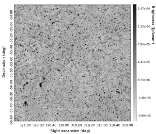
Figure 1: $2^{\circ}\times 2^{\circ}$ central cutout of an EMU pilot tile.

3.2 Processing Speeds

In the course of our analyses we were able to use Hydra to assess and compare the processing speeds of the different SFs. Table 2 shows order of magnitude CPU times for one PRD calculation step, during the optimisation process (Paper I).

Table 2: SF order of magnitude PRD CPU times (rounded to one significant figure) for CMP, EXT, and EMU images. The processing was done on a 2GHz 16 core (single threaded) Intel Xeon Processor with 60G of RAM running Ubuntu 20.04.3 LTS.

	PRD CPU Time (s)
SF	CMP	EXT	EMU
Aegean	300	600	200
Caesar	1 000	4 000	500
ProFound	90	90	40
PyBDSF	90	90	40
Selavy	1 000	4 000	3 000

Table 3: Typhon run statistics for $2^{\circ}\times 2^{\circ}$ CMP and EXT and EMU images, with SF, image depth ($\mbox{D}=\mathcal{D},\,\mathcal{S}$), RMS parameter ($n_{rms}$ [$\sigma$]) island parameter, ($n_{island}$ [$\sigma$]), source numbers (N), residual RMS [$\mu$Jy/beam], and residual MADFM (median absolute deviation from the median) [$\mu$Jy/beam] columns.^a The CMP and EXT results are reproduced from Paper I.

SF	D	CMP Sources					EXT Sources					EMU Sources
		$n_{rms}$	$n_{island}$	N	RMS	MADFM	$n_{rms}$	$n_{island}$	N	RMS	MADFM	$n_{rms}$	$n_{island}$	N	RMS	MADFM
Aegean	$\mathcal{D}$	3.074	3.070	6 016	20.0	19.0	3.074	3.070	4 112	67.0	56.0	2.676	2.674	8 538	91.0	26.0
Caesar	$\mathcal{D}$	3.074	3.000	4 084	19.0	16.0	3.206	3.000	3 618	54.0	44.0	2.809	2.806	7 838	27.0	23.0
ProFound	$\mathcal{D}$	2.412	2.409	4 997	18.0	16.0	2.412	2.409	3 730	52.0	43.0	2.279	2.277	11 484	24.0	19.0
PyBDSF	$\mathcal{D}$	2.809	2.806	5 991	22.0	19.0	2.809	2.806	4 688	106	54.0	2.941	2.938	8 292	1080	26.0
Selavy	$\mathcal{D}$	3.206	3.203	3 225	45.0	20.0	3.206	3.203	2 544	982	58.0	2.941	2.938	5 880	566	27.0
Aegean	$\mathcal{S}$	3.868	3.864	747	110	110	3.603	3.599	1 287	321	317	3.603	3.599	926	192	169
Caesar	$\mathcal{S}$	4.000	3.000	657	109	106	3.603	3.000	1 297	310	295	3.735	3.000	885	169	166
ProFound	$\mathcal{S}$	3.074	3.070	642	109	107	2.941	2.938	1 138	311	298	3.735	3.732	778	169	165
PyBDSF	$\mathcal{S}$	3.735	3.732	598	111	109	3.338	3.335	1 312	316	313	3.735	3.732	794	409	169
Selavy	$\mathcal{S}$	4.000	3.996	427	114	110	3.735	3.732	787	623	320	3.603	3.599	789	169	169
$\!\!{}^{a}$The MADFM estimators are normalised by 0.6744888 (Whiting, 2012).

The wide range in CPU times is due to the background and noise estimators being used. For Caesar and Selavy we are using robust statistics (Whiting & Humphreys, 2012; Riggi et al., 2016, Paper I), which has time complexity (Knuth, 2000) $\mathcal{O}(n\,\log\,n)$. Aegean also has the same time complexity, however it uses an Inter-Quartile Range (IQR) estimator (Hancock et al., 2012). PyBDSF uses the typical $\mu/\sigma$ estimator (Mohan & Rafferty, 2015), which goes as $\mathcal{O}(n)$. ProFound uses $\sigma$-clipping (Robotham et al., 2018), which is also of that order. The CPU times can be seen to vary, sometimes significantly, between images.

3.3 Typhon Statistics

3.3.1 Optimisation Run Results

Hydra’s Typhon software module (Paper I) was used to optimise Aegean, Caesar, ProFound, PyBDSF, and Selavy’s RMS and island parameters to a 90% PRD cutoff (Table 3). Aegean, PyBDSF, and Selavy RMS box parameters were pre-optimised (Table 4) using bane (Hancock et al., 2018) as part of a process to minimise the mean noise (i.e., $\mu$-optimisation, Paper I). Here we present the EMU $\mathcal{D/S}$-image results, with relevant CMP and EXT image results from Paper I incorporated as appropriate for comparison.

Table 4: Hydra $\mu$-optimised Aegean, PyBDSF, and Selavy box_size and step_size input parameters,^a for CMP, EXT, and EMU $\mathcal{D}/\mathcal{S}$-images. The CMP and EXT results have been incorporated from Paper I.

Image	Image	$\mu$	box_size	step_size
Type	Depth	($\mu$Jy/beam)	(′′)	(′′)
CMP	$\mathcal{D}$	21.81	240	120
	$\mathcal{S}$	108.2	180	88
EXT	$\mathcal{D}$	68.01	480	240
	$\mathcal{S}$	325.3	240	120
EMU	$\mathcal{D}$	35.28	720	270
	$\mathcal{S}$	171.23	216	80
$\!\!{}^{a}$Selavy only accepts box_size.

Table 3 summarises the Typhon run statistics for our image data. As noted in Paper I, the RMS and island parameters are similar for CMP and EXT $\mathcal{D}$-images for a given SF; however, they are slightly lower for the real $\mathcal{D}$-image. As for the $\mathcal{S}$-image, the simulated and real parameters are similar.

Table 4 summarizes the EMU $\mathcal{D/S}$-image optimized RMS box parameters for Aegean, PyBDSF, and Selavy. First, we note that $\mu_{\mathcal{S}}/\mu_{\mathcal{D}}\sim 5$ for all images. This is consistent with the factor of 5 noise increase for the $\mathcal{S}$-image. Secondly, $\mu^{\mbox{\tiny EMU}}_{\mathcal{D}}\sim 35\,\mu$Jy/beam falls between $\mu^{\mbox{\tiny CMP}}_{\mathcal{D}}\sim 22\,\mu$Jy/beam and $\mu^{\mbox{\tiny EXT}}_{\mathcal{D}}\sim 68\,\mu$Jy/beam (and similarly for $\mathcal{S}$-images), suggesting the simulated images are well suited for our analysis.

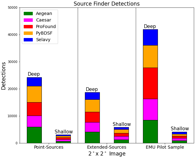
Figure 2: SF CMP, EXT, EMU $\mathcal{D/S}$-image detection stacked plots (from the N columns of Table 3).

Figure 2 shows stacked measures of $\mathcal{D/S}$ source detections (N) for the $\mathcal{D/S}$-images, where we have included the simulated data from Paper I. For the $\mathcal{S}$-images, for a given SF, N is similar between the CMP and EMU sources, but slightly higher for EXT sources. With the exception of Selavy, N is similar between SFs. As for the simulated $\mathcal{D}$-images, the relative proportion of N between SFs is roughly the same for CMP and EXT sources, except for Selavy. In the EMU image there is a significant increase in the relative proportion of N by ProFound. This suggests a possible excess of spurious detections, an increase in real detections missed by other SFs, real detections being split into more components than by other SFs, or a combination of these.

Table 5: $\mathcal{S:D}$ recovery rates.

SF	CMP	EXT	EMU
Aegean	12.4%	31.3%	10.8%
Caesar	16.1%	35.8%	11.3%
ProFound	12.8%	30.5%	6.8%
PyBDSF	10.0%	28.0%	9.6%
Selavy	13.2%	30.9%	13.4%

In Paper I we examined the ratios of deep-to-injected ($\mathcal{D:J}$) and shallow-to-deep ($\mathcal{S:D}$) source detections, or recovery rates. Table 5 shows the $\mathcal{S:D}$ recovery rates for our image data. The $\mathcal{S:D}$ recovery rates are roughly of the same order between the CMP and EMU images, indicating the real image has a large population of compact sources (c.f. Figure 1). The recovery rate is higher for the EXT image, by a factor around $2-3$, likely a reflection of the different flux density distribution of sources in this image. This would seem to suggest that the CMP image more closely models our real sample. This is also evident when the real image (Figure 1) is compared with the simulated images in Paper I.

Table 6: $\mathcal{D/S}$ (D) residual (res.) $|\mbox{RMS}-\mbox{MADFM}|/\mbox{MADFM}$ (%), RMS [$\mu$Jy/beam], and MADFM [$\mu$Jy/beam] statistics extracted from Table 3.

SF/Res.	D	CMP	EXT	EMU
Aegean	$\mathcal{D}$	5.3%	19.6%	250.0%
Caesar	$\mathcal{D}$	18.8%	22.7%	17.4%
ProFound	$\mathcal{D}$	12.5%	20.9%	26.3%
PyBDSF	$\mathcal{D}$	15.8%	80.4%	58.5%
Selavy	$\mathcal{D}$	125.0%	69.3%	109.6%
RMS	$\mathcal{D}$	$24.8\pm 10.2$	$56.4\pm 28.2$	$41.9\pm 28.8$
MADFM	$\mathcal{D}$	$18.0\pm 1.7\;\;$	$51.0\pm 6.3\;\;$	$24.2\pm 2.9\;\;$
Aegean	$\mathcal{S}$	0.0%	1.3%	13.6%
Caesar	$\mathcal{S}$	2.8%	5.1%	1.8%
ProFound	$\mathcal{S}$	1.9%	4.4%	2.4%
PyBDSF	$\mathcal{S}$	1.8%	1.0%	142.0%
Selavy	$\mathcal{S}$	3.6%	94.7%	0.0%
RMS	$\mathcal{S}$	$110.6\pm 1.9$	$376.2\pm 123.5$	$221.6\pm 94.1$
MADFM	$\mathcal{S}$	$108.4\pm 1.6$	$308.6\pm 10.2\;\;$	$167.6\pm 1.7\;\;$

For simulated and real images there is some variability in the residual RMS values, with Selavy being consistently high for $\mathcal{D}$-images and consistently low for $\mathcal{S}$-images. On the whole, however, the residual MADFMs are consistent between all SFs for a given image. Table 6 summarises these results. The $|\mbox{RMS}-\mbox{MADFM}|/\mbox{MADFM}$ percentage differences are a measure of the robustness of the SF residual models (which is also reflection of the Hydra optimisation schema, Paper I).

3.3.2 Source Size Distributions

Figure 3 shows the major-axis distribution for the EMU image data. Both the $\mathcal{D}$ and $\mathcal{S}$ source detections are combined, as the $\mathcal{S}$ data provides additional information. Although the underlying sources are in common between $\mathcal{D}$ and $\mathcal{S}$, the higher noise level means that the SFs are operating on quantitatively different pixel values, and may well derive different size estimates. Also, the numbers of detections for $\mathcal{S}$ are relatively small (Figure 2), so incorporating them here is unlikely to bias the results. Recall that size estimates for different SFs use different methods and are not necessarily directly comparable.

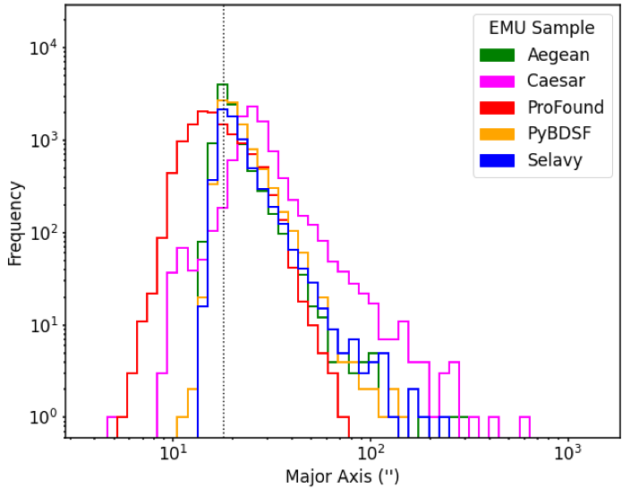
Figure 3: Major-axis distributions for EMU sources (showing size distributions from both $\mathcal{D}$ and $\mathcal{S}$ image measurements together). NB: Size estimates between SFs are not necessarily directly comparable as they are estimated using different methods (Paper I).

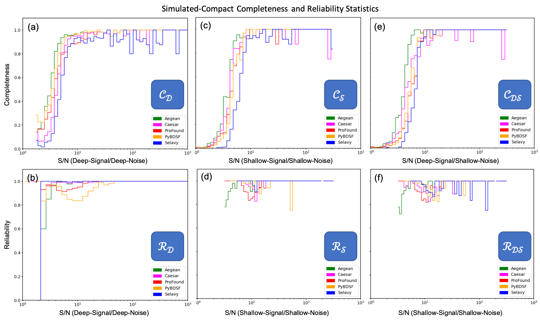
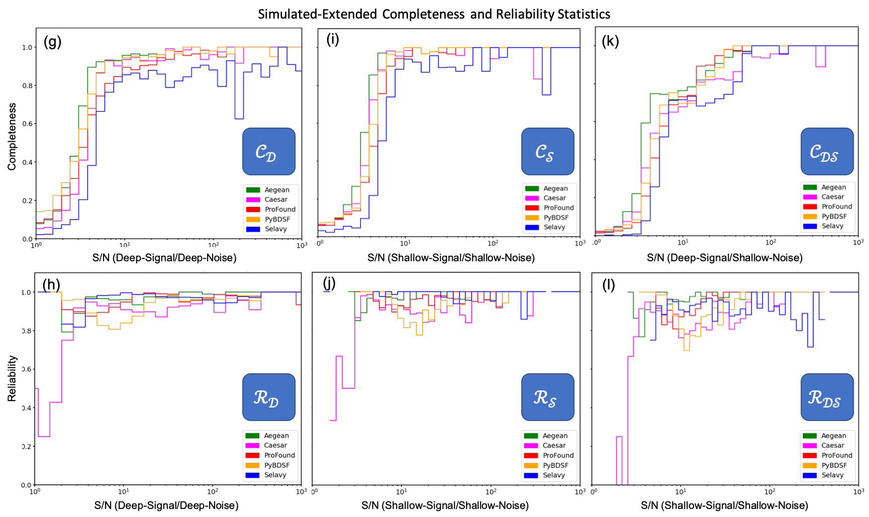
Figure 4: CMP and EXT $\mathcal{C_{D}}$ (a and g), $\mathcal{R_{D}}$ (b and h), $\mathcal{C_{S}}$ (c and i), $\mathcal{R_{S}}$ (d and j), $\mathcal{C_{DS}}$ (e and k), and $\mathcal{R_{DS}}$ (f and l) vs. S/N. These results are reproduced from Paper I, Figures 14, 15, and 16.

In Figure 3, all but one of the distributions peak at the scale corresponding to the beam size, consistent with point (i.e., compact) source detections. Caesar shows a distribution systematically offset by a factor of about 1.5 toward larger sizes. The results for Aegean, PyBDSF, and Selavy are similar, which is reassuring given that they use similar approaches in fitting elliptical Gaussians to source components (see Paper I). ProFound shows an excess of very small sources. Some of these will be due to noise spikes, and others to faint sources close to the detection threshold (Table 3) where ProFound only has a few pixels available from which to calculate its flux-weighted sizes, leading to underestimates. Caesar’s excess at small sizes is less than that from ProFound, although were the Caesar results to be shifted left by the factor 1.5 noted above, it would be roughly comparable. The origin of small sizes reported by Caesar might be due to deblending issues, as it has a relatively lower source detection number (Figure 2). In general, all SFs with detections below the beam size are expected to be contaminated, to some degree, by noise spikes.

As for EXT images, they have a similar behaviour to the EMU case, except to a lesser degree (Paper I). In the CMP case, there are significantly fewer detections below the beam size, with some overestimates of source sizes in the case of ProFound and PyBDSF. The overestimates are most likely due to nearby noise peaks being incorporated into a source fit, artificially enlarging the size.

3.4 Completeness and Reliability

In Paper I we explored $\mathcal{C_{D}}$ (and $\mathcal{C_{S}}$) and $\mathcal{R_{D}}$ (and $\mathcal{R_{S}}$) for CMP and EXT sources; for ease of discussion and comparison here, we have duplicated the relevant results in Figure 4, along with the new measurements from the EMU data in Figure 5. Aegean was found to have the best $\mathcal{C}$ statistic followed PyBDSF, ProFound, Caesar, and Selavy. Selavy, followed by Caesar, tended to miss bright sources, and were less reliable ($\mathcal{R}$) at high S/N. In general, the statistics for all SFs are poorer for the EXT case, but followed the same performance trends as the CMP case. Some of this can been attributed to confusion.

Figure 5 shows the newly measured $\mathcal{C_{DS}}$ and $\mathcal{R_{DS}}$ metrics for the EMU image. The results are similar to the CMP image case (Figure 4). Here, the detections appear fairly complete for all SFs, with high completeness ($\mathcal{C_{DS}}\gtrsim 0.9$) above $\mbox{S/N}\gtrsim 10$ dropping to $\mathcal{C_{DS}}\sim 0.5$ by $\mbox{S/N}\sim 5$. Reliability is also generally high ($\mathcal{R_{DS}}\gtrsim 0.9$) for most SFs, although Selavy’s performance here is notably poorer ($0.7\lesssim\mathcal{R_{DS}}\lesssim 0.9$) across almost the full range of S/N. All SFs drop in reliability below $\mbox{S/N}\sim 10-20$.

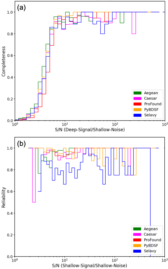
Figure 5: EMU-image $\mathcal{C_{DS}}$ vs. S/N (a) and $\mathcal{R_{DS}}$ (b) vs. S/N, with S/N expressed as $\mathcal{D}$-signal/$\mathcal{S}$-noise and $\mathcal{S}$-signal/$\mathcal{S}$-noise, respectively.

3.5 Flux Density Ratios and $n\sigma$ Scatter

Figure 6 shows the flux ratios, $S_{out}/S_{in}$, for each of the SFs. For the simulated images, $S_{in}$ (expressed as S/N) represents the $\mathcal{J}$-signal over the $\mathcal{D}$-noise. For the real images it represents the $\mathcal{D}$-signal over the $\mathcal{S}$-noise. $S_{out}$ represents the detected measurement. The horizontal (dotted) lines represent $S_{out}=S_{in}$, and the solid and dashed curves about these lines are the $1\sigma$ and $3\sigma$ deviations from $S_{in}$, respectively. The dot-dashed curves are the detection thresholds (i.e., the RMS parameters, $n_{rms}$, in Table 3, corresponding to 90% PRD), and the dotted curves represent nominal $5\sigma$ thresholds (c.f. Hopkins et al., 2015). The sharp vertical cut off below $\mbox{S/N}\sim 2$ for the CMP images is a consequence of having no artificial input sources fainter than that level.

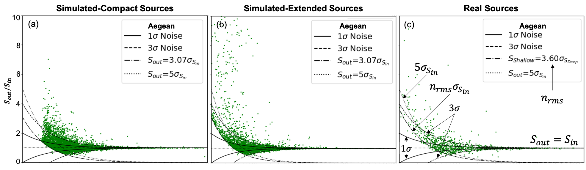
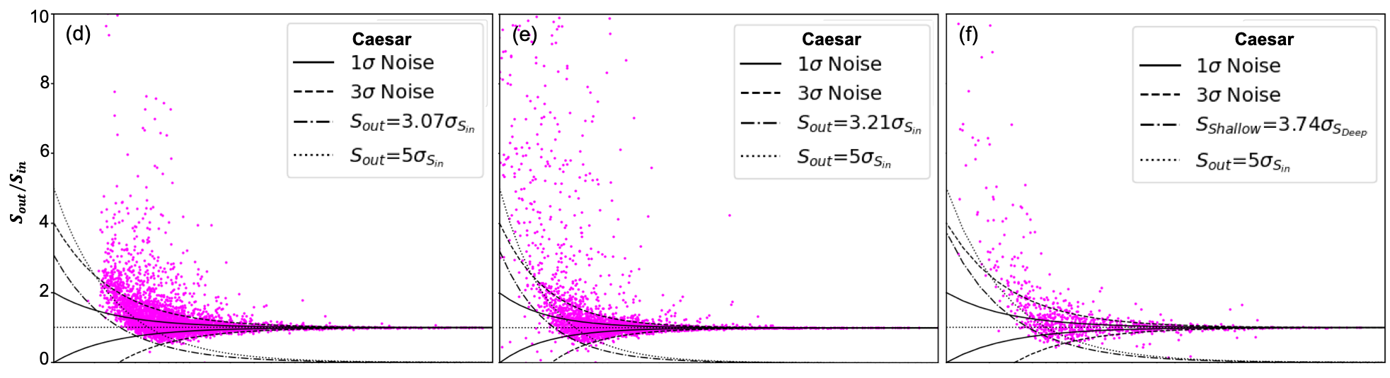
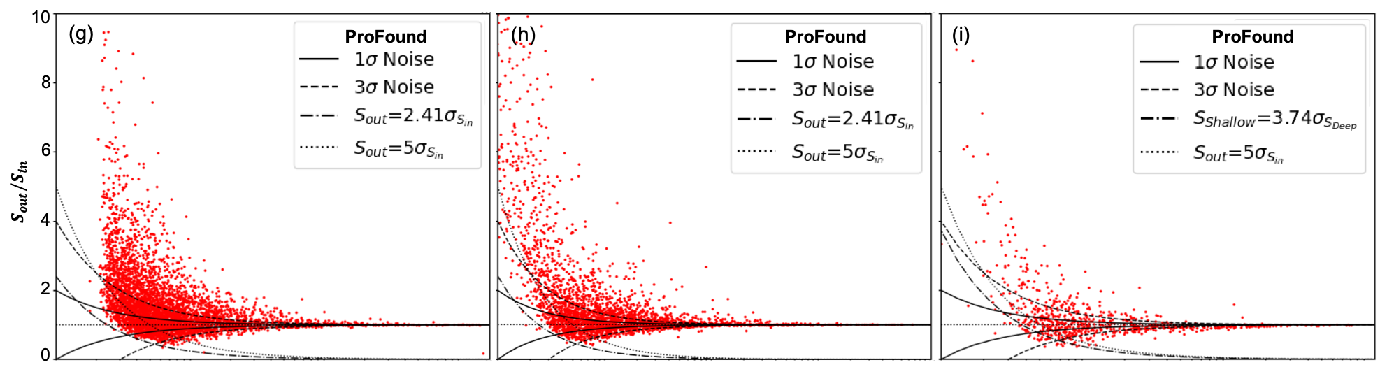
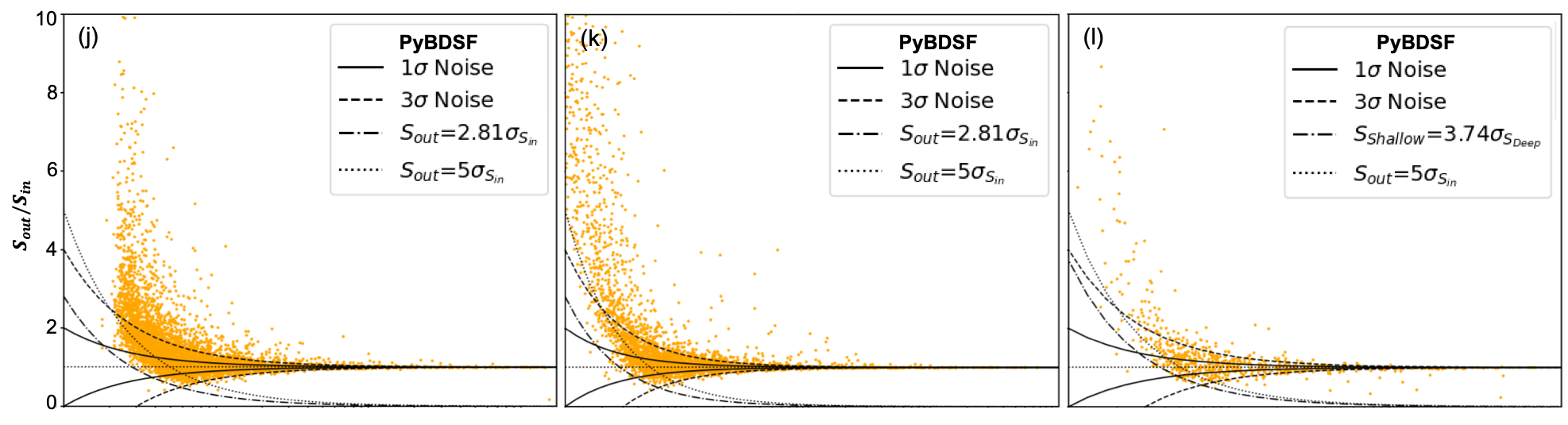
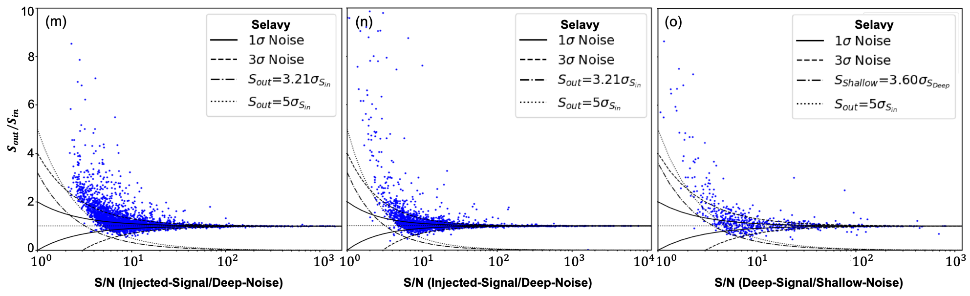
Figure 6: Flux density ratios ($S_{out}/S_{in}$) for CMP (left), simulated-extended (middle), and real (right) sources for Aegean (a, b, and c), Caesar (c, e, and f), ProFound (g, h, and i), PyBDSF (j, k, and l) and Selavy (m, n, and o) vs. S/N, expressed as $\mathcal{J}$-signal/$\mathcal{D}$-noise and $\mathcal{D}$-signal/$\mathcal{S}$-noise for simulated and real sources, respectively. The $1\sigma$ (solid) and $3\sigma$ (dashed) curves are RMS noise ($\sigma$) deviations from the $\mbox{flux-ratio}=1$ lines (dotted). Also shown are the detection threshold ($n_{rms}$; dot-dashed curves) and nominal $5\sigma$ threshold (dotted curves). These curves are annotated in (c).

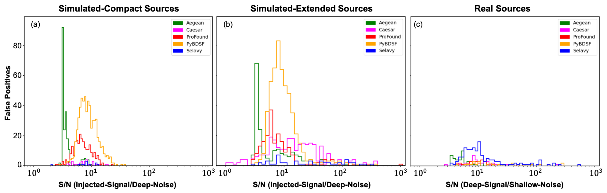
Figure 7: False positives vs. S/N for CMP (a), EXT (b), and real (c) sources, with S/N expressed as $\mathcal{J}$-signal/$\mathcal{S}$-noise and $\mathcal{D}$-signal/$\mathcal{S}$-noise for simulated and real sources, respectively.

Table 7: $3\sigma$ scatter ($s_{3\sigma}(\hat{S}_{i})$, Equation 2) at $\hat{S}_{i}=3,\,5,\,10$, for SF CMP, EXT, and EMU source flux density ratios (Figure 6). Also shown are averaged $3\sigma$ scatters.

	$3\sigma$ Scatter									Averaged $3\sigma$ Scatter
	CMP			EXT			EMU			$\langle[s_{3\sigma}(3),\,s_{3\sigma}(5),\,s_{3\sigma}(10)]\rangle$
SF	$s_{3\sigma}(3)$	$s_{3\sigma}(5)$	$s_{3\sigma}(10)$	$s_{3\sigma}(3)$	$s_{3\sigma}(5)$	$s_{3\sigma}(10)$	$s_{3\sigma}(3)$	$s_{3\sigma}(5)$	$s_{3\sigma}(10)$	CMP	EXT	EMU
Aegean	3.49%	3.91%	4.27%	9.20%	7.98%	7.48%	3.40%	4.88%	5.59%	3.89 $\pm$ 0.32%	8.22 $\pm$ 0.72%	4.62 $\pm$ 0.91%
Caesar	6.93%	7.11%	6.65%	11.02%	9.92%	9.08%	4.62%	4.33%	6.76%	6.90 $\pm$ 0.19%	10.01 $\pm$ 0.79%	5.24 $\pm$ 1.08%
ProFound	14.55%	16.70%	21.74%	14.20%	15.93%	20.28%	6.60%	6.94%	10.72%	17.66 $\pm$ 3.01%	16.80 $\pm$ 2.56%	8.09 $\pm$ 1.87%
PyBDSF	8.85%	6.20%	6.64%	10.80%	9.55%	9.57%	3.43%	3.18%	5.88%	7.23 $\pm$ 1.16%	9.97 $\pm$ 0.58%	4.16 $\pm$ 1.22%
Selavy	6.43%	6.92%	6.63%	10.25%	8.91%	9.06%	3.94%	3.77%	5.99%	6.66 $\pm$ 0.20%	9.41 $\pm$ 0.60%	4.57 $\pm$ 1.01%

The form of the flux ratio diagrams for the EMU image follow that of the simulated images, however its $\mathcal{DS}$ source numbers are lower due to relying on detections in the $\mathcal{S}$-image. Similar $\mathcal{DS}$ flux ratio statistics can be measured for the simulated cases (not shown). We use $\mathcal{D}$ diagnostics for the simulated images, as they are the most robust, whereas the $\mathcal{S}$ and $\mathcal{DS}$ metrics provide no extra useful information.

For the simulated cases all SFs, with the exception of Selavy, are seen to detect sources down to the specified RMS threshold (dot-dashed line). Selavy was given a $\sim 3.2\sigma$ threshold (Table 3), but only appears to recover sources down to a $5\sigma$ level (Figure 6 (m) and (n)). For the real image case, though, Selavy does appear to recover sources down to the nominal S/N threshold.

Figure 7 is a complementary diagnostic to Figure 6, and shows the corresponding false-positive distributions. This emphasises in another way the SF characteristics we have seen in earlier $\mathcal{R}$ distributions (§ 3.4). Specifically, for CMP sources (i.e., comparing Figures 4b and 7a), Aegean picks up false detections predominantly close to the S/N threshold, with ProFound and PyBDSF having false detections peaking between about S/N$\sim 5-10$, arising from blended sources and overestimated source sizes. The false sources seen by each SF correspond to their deficit in $\mathcal{R}$ (Figure 4 and Figure 5). In particular, Aegean displays higher levels of completeness, but at the expense of reliability at low S/N, with the converse being true for Selavy and Caesar. In this analysis, Aegean shows arguably the best performance, as is evident from its false-positive distribution being limited to low S/N, generally reliable flux densities seen in the limited scattering beyond $S_{out}/S_{in}>3\sigma$, and good completeness to low S/N. This is not surprising, though, as Aegean is well designed for identifying and fitting point sources, and the simulated data used here do not include anything else.

The false-positive distributions for the EXT case (cf., Figures 4h and 7b) have similar characteristics to the CMP case (Figures 4b and 7a), but are broadened somewhat. As for the real case (Figure 7c), the distribution for Selavy becomes more prominent, as reflected in its $\mathcal{R_{DS}}$ (Figure 5b).

Pleasingly, none of the SFs show any systematic overestimate or underestimate of the flux densities (Figure 6). To quantify the reliability of the flux density measurements, we focus on the scatter in the distribution of $S_{out}/S_{in}$ as a function of S/N. We first define the fraction of sources $r_{n\sigma}(\hat{S}_{i})$ above a S/N limit, $\hat{S}_{i}$, with $S_{out}/S_{in}$ lying between $1-n\sigma$ and $1+n\sigma$:

$$r_{n\sigma}(\hat{S}_{i})=\frac{\displaystyle\left|\left\{\!\frac{S_{out}}{S_{in}}\!\left|1\!\!-\!\!\frac{n}{\hat{S}_{in}}\!\leq\!\frac{S_{out}}{S_{in}}\!\leq 1\!+\!\!\frac{n}{\hat{S}_{in}}\!\ni\!\hat{S}_{in}\!\geq\!\hat{S_{i}}\right.\!\right\}\right|}{\displaystyle\left|\left\{\!\frac{S_{out}}{S_{in}}\!\left|\hat{S}_{in}\!\geq\!\hat{S_{i}}\!\right.\right\}\right|}\,,$$ (1)

where $S$ represents flux density, and $\hat{S}$ represents S/N. Using this, we define the scatter in $S_{out}/S_{in}$ outside an $n\sigma$ range as

$$s_{n\sigma}(\hat{S}_{i})=1-r_{n\sigma}(\hat{S}_{i})\,.$$ (2)

Table 7 shows the compiled statistics for $3\sigma$ scatter.

For the CMP case, Aegean and Selavy tend to show the least scatter. The scatter for PyBDSF and Selavy is slightly higher than that reported by Hopkins et al. (2015), who saw scatters above a $5\sigma$ detection threshold of 4.9% for PyBDSF and 3.3% for Selavy, compared to the values of $\sim 6\%$ seen here.

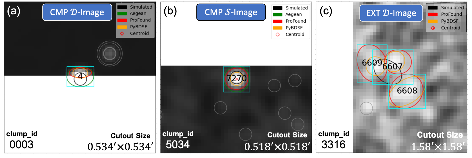
Figure 8: Edge Detection Infographic: Edge detection example cutouts for (a) CMP $\mathcal{D}$-image (from the $\mbox{S/N}\sim 1\,600\pm 110$ bin of $\mathcal{C_{D}}$, Figure 4a), (b) CMP $\mathcal{S}$-image (from the $\mbox{S/N}\sim 42.6\pm 2.9$ bin of $\mathcal{C_{S}}$, Figure 4c), and (c) EXT $\mathcal{D}$-image (from the $\mbox{S/N}\sim 0.318\pm 0.036$ bin of $\mathcal{C_{D}}$, Figure 4g). In examples (a) and (b), Caesar and Selavy failed to detected the injected sources at match_ids 4 and 7270, respectively. In example (c), there is an injected source at match_id 6607 ($\mbox{S/N}\sim 0.34$) which is detected by ProFound ($\mbox{S/N}\sim 4.82$) and PyBDSF ($\mbox{S/N}\sim 6.39$). The remaining detections, by both SFs, at match_ids 6608 and 6609 are spurious, due to noise fluctuations.

On the whole, the scatter is comparable between the CMP and EMU sources, with the highest scatter for EXT sources. Aegean tends to deliver the least scatter in the flux density estimates, with Caesar, PyBDSF, and Selavy showing similar results at the next level, and ProFound always with the highest scatter. The results in the EMU image appear to show the least scatter overall, but recall that these measurements result from comparing the detections in the $\mathcal{S}$-image against those in the $\mathcal{D}$-image for each SF against itself. These are not directly comparable with simulated image cases where the scatter compares measured against known input values. The implication here is that flux density estimates inferred from $\mathcal{D}/\mathcal{S}$ comparisons may not reflect the full extent of the true underlying uncertainties.

3.6 Hydra Viewer Cutout Case Studies

Here we present a gallery of Hydra Viewer cutouts, for the purpose of analysing frequently encountered anomalies and artifacts utilising the metrics explored in the previous subsections. They have been sorted into broad categories: edge detections (sources near image edges), blending/deblending, faint sources, component size errors, bright sources, and diffuse emission. With the exception of diffuse emission (seen only in the real image), all such artefacts are found in the SF catalogues in all of the images, to varying degrees.

3.6.1 Edge Detections

Detecting sources at or near the edges of images is problematic, as it can be difficult to estimate the noise and sometimes the source itself is truncated. For sources truncated near an edge, Aegean tends to extrapolate their shape, while ProFound estimates the remaining flux, and PyBDSF treats them as complete sources: e.g., for the CMP source in Figure 8a, Caesar and Selavy do not record this source, and hence it contributes to an underestimate of $\mathcal{C_{D}}$ at $\mbox{S/N}\sim 1\,600\pm 110$ for those finders (Figure 4a). Here S/N $\sim$ 1 519 for the injected source, and 621, 263, and 277 for Aegean, ProFound, and PyBDSF, respectively. So the source flux-density is underestimated. This does not appear as degradation in $\mathcal{C_{D}}$, but is reflected in the scatter of the flux-ratio (Figure 6).

SF performance is better when sources are just touching an edge: e.g., for the CMP source in Figure 8b. Here again Caesar and Selavy do not report this source, which falls in the $\mathcal{C_{S}}$ $\mbox{S/N}\sim 42.6\pm 2.9$ bin (Figure 4a). The other finders detect it and estimate the flux density for this source reliably. The injected source S/N is $\sim$ 41.66, and it is measured at 44.82, 44.92, and 45.19 for Aegean, ProFound, and PyBDSF, respectively.

Figure 8c shows an example of noise spikes appearing as low S/N detections, surrounding an $\mbox{S/N}\sim 0.34$ EXT source, near an edge. Only ProFound and PyBDSF make detections, and only in the $\mathcal{D}$-image. There is little difference in apparent flux density between the injected source detection at match_id 6607 and the spurious adjacent detections at match_ids 6608 and 6609.

A cursory scan suggests Caesar finds sources at image edges less often than other SFs, and Selavy tends not to identify them at all. Most likely, the island is there, but the fit has failed and no source component is recorded. As ProFound is capable of characterising irregularly shaped objects it tends to perform well for such truncated sources.

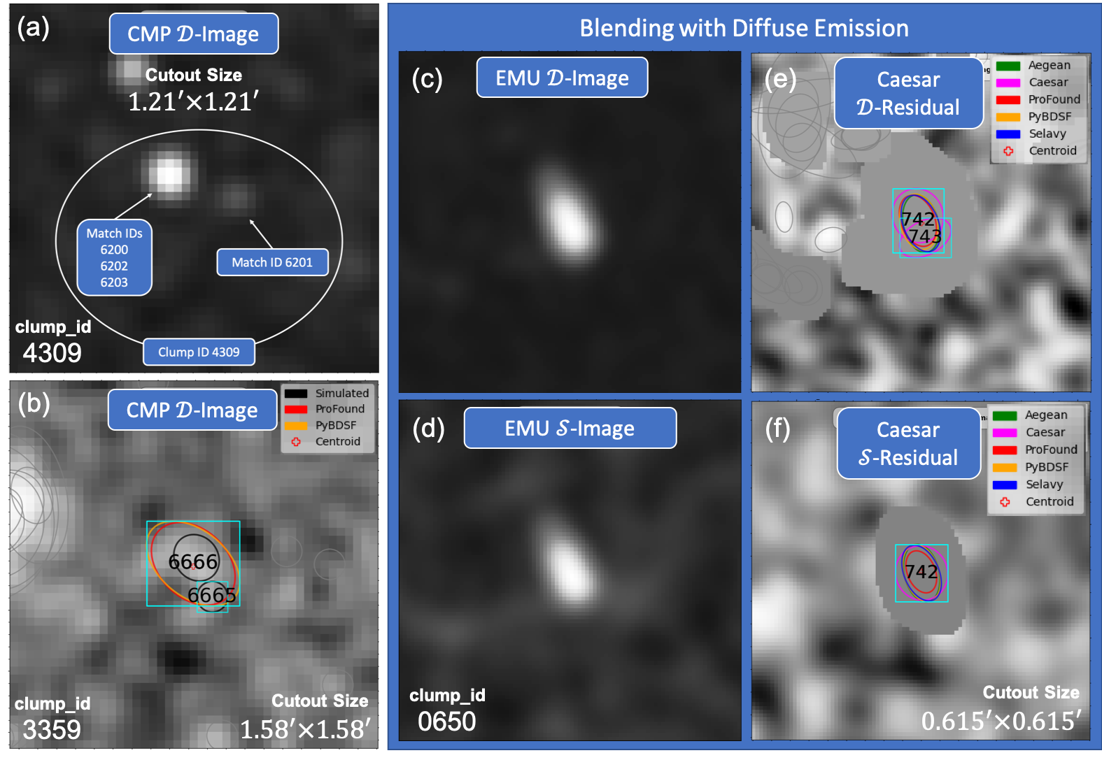
Figure 9: Blended Sources Infographic: CMP (a–b) and real (EMU; c–f) $\mathcal{D}$-image examples of blended sources. In example (a) (from the $\mbox{S/N}\sim 19.6\pm 1.3$ bin of $\mathcal{C_{D}}$, Figure 4a), only ProFound missed detection of the isolated source at match_id 6201. The remaining injected sources overlap to make up a single unresolved compact object, which is identified as match_id 6203 by all SFs. In example (b) (from the $\mbox{S/N}\sim 0.318\pm 0.036$ bin of $\mathcal{C_{D}}$, Figure 4a), there are two injected sources at match_ids 6665 ($\mbox{S/N}\sim 0.070$) and 6666 ($\mbox{S/N}\sim 0.336$). Only match_id 6666 is detected by ProFound ($\mbox{S/N}\sim 7.468$) and PyBDSF ($\mbox{S/N}\sim 12.446$). Examples (c) and (d) show a $\mathcal{D}$-image and $\mathcal{S}$-image cutouts, respectively, of a compact object with a diffuse tail. Only Caesar is able to resolve the $\mathcal{D}$-image (into two components; top), but not the $\mathcal{S}$-image (bottom) as the diffuse emission is washed out. Examples (e) and (f) are the corresponding a $\mathcal{D}$-residual and $\mathcal{S}$-residual image cutouts in the previous example, respectively, for Caesar. All SFs make $\mathcal{D}$ and $\mathcal{S}$ detections at match_id 742. Caesar separately detects the bright peak at match_id 743 in the $\mathcal{D}$-image, but with no corresponding $\mathcal{S}$ match. This contributes to a reduction in the inferred $\mathcal{C_{DS}}$ for Caesar at $\mbox{S/N}\sim 3.4$ in Figure 5a.

3.6.2 Blended Sources

For the simulated images there are example cases of unresolved compact sources: e.g., Figure 9a. Here match_ids 6200, 6202, and 6203, with injected flux densities of 0.0529, 0.4032, and 0.6928 mJy, respectively, appear as a single compact unresolved source. All SFs detect it, with measured flux densities of 1.1118, 1.1113, 1.2481, 1.1296, and 1.1230 mJy, for Aegean, Caesar, ProFound, PyBDSF, and Selavy, respectively. These values are consistent with the total injected flux $\sim 1.1489\,$mJy. So the total flux is accounted for. Regardless, this causes a degradation in the $\mathcal{C_{D}}$; in particular, the $\mbox{S/N}\sim 20$ bin of Figure 4a.

Blending is also encountered with overlapping point and extended sources, with the former having slightly lower S/N. Figure 9b shows an example of a very low S/N detection being influenced by an even fainter adjacent source. Here, only ProFound and PyBDSF, which have the lowest detection thresholds (Table 3), make detections, and only in the $\mathcal{D}$-image. Both SFs treat the two adjacent injected sources as a single source. This leads to a degradation in $\mathcal{C_{D}}$, but not $\mathcal{R_{S}}$ (Figure 4a–b).

For simple cases of real sources with diffuse emission, such as a compact object with a diffuse tail, Aegean, ProFound, PyBDSF, and Selavy tend to characterise them with a single flux-weighted component position, whereas Caesar tends to resolve them in $\mathcal{D}$-images, but not $\mathcal{S}$-images where the diffuse emission is diminished: e.g., Figure 9c–f. Here Caesar decomposes this object into two sources in the $\mathcal{D}$-image (e), but not in the $\mathcal{S}$-image (f). The remaining SFs detect this as a single source in both the $\mathcal{D}$ and $\mathcal{S}$ images. The diffuse emission is washed out in the $\mathcal{S}$-image, leading to a slight ($\sim 3$%) drop in the overall S/N.

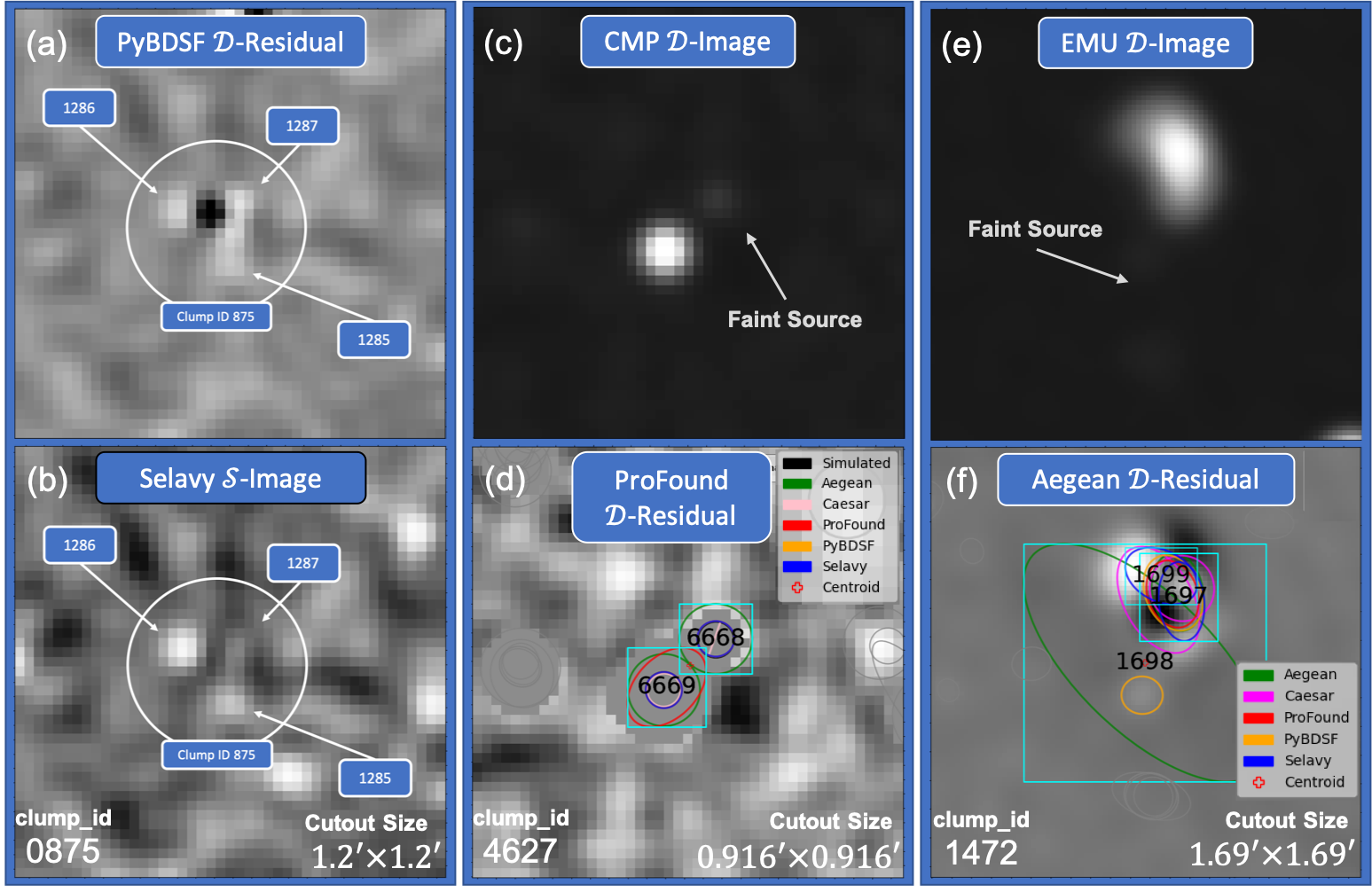
Figure 10: Deblending Issues Infographic: CMP PyBDSF $\mathcal{D}$-residual-image (a) with Selavy $\mathcal{S}$-residual-image (b) (from clump_id 875), CMP $\mathcal{D}$-image (c) with ProFound $\mathcal{D}$-residual-image (d) (from clump_id 4672), and real (EMU) $\mathcal{D}$-image (e) with Aegean $\mathcal{D}$-residual-image (f) (from clump_id 875) cutout examples of deblending issues. In example (a), only PyBDSF makes a detection at match_id 1287. In example (b), only Selavy makes a detection at match_id 1287. In example (c–d), ProFound provides a single flux-weighted component that blends these two adjacent sources, and which is best matched to match_id 6669. This leads to the result that match_id 6668 is deemed undetected in the $\mathcal{C_{D}}$ statistics (Figure 4a). In example (e–f), Aegean overestimates the extent of the vary faint (diffuse) source at match_id 1698 (bottom image, middle): i.e., $(a,b,\theta)\sim(130^{\prime\prime},\,57.6^{\prime\prime},\,45.8^{\circ})$, with major, minor, and position-angle components, respectively. There is no corresponding $\mathcal{S}$ match. This leads to a degradation in the $\mathcal{C_{DS}}$ S/N $\sim$ 25 bin of Figure 5a.

3.6.3 Deblending Issues

Deblending issues can occur in systems having a relatively low S/N neighbour to a brighter object, causing a positional fit which is offset from the true centre of the bright object: e.g., Figure 10a. This leads to a degradation in $\mathcal{R_{D}}$ (and $\mathcal{R_{DS}}$). In such cases, PyBDSF tends to bias its position estimates towards flux-weighted centers. The other SFs tend to be less biased in such a fashion: e.g., Figure 10b. ProFound tends to extend its component footprint to include faint sources: e.g., Figure 10d.

Figure 11 shows an example of an injected source with a flux density of $\sim 291\,\mu$Jy which is erroneously measured by Caesar as $\sim 0.664\,\mu$Jy. This is likely to be a consequence of a poor deblending of the two adjacent sources, initially identified by Caesar as a single island. The position is accurate, so it is counted as a correct match, but because $\mathcal{R_{D}}$ (Figure 4b) is calculated using the measured S/N, this source contributes to $\mathcal{R_{D}}$ at the unreasonably low value of $\mbox{S/N}\sim 0.033$. For this source, Aegean, PyBDSF, and Selavy correctly estimate the flux density as $281.9^{+4.2}_{-8.4}\,\mu$Jy, and it contributes to $\mathcal{R_{D}}$ for those SFs at $\mbox{S/N}\sim 12$. It is worth noting here that requiring flux-density matching in the reliability metric calculation would lead (for Caesar) to this source being deemed a false detection, although it has been detected at the correct location. ProFound does not separately detect match_id 6668 (Figure 10d) as it has blended it with match_id 6669. Comparing Figure 11 and 10d we can see the similar islands detected by ProFound and Caesar, although ProFound’s boundary is tighter, which provides a clear indication of why only a single match was identified.

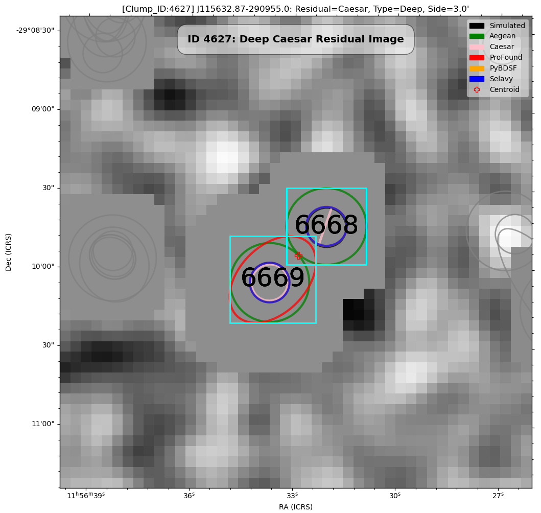
Figure 11: Caesar clump_id 4627 $\mathcal{D}$ $0.916^{\prime}\times 0.916^{\prime}$ residual-image cutout for simulate-compact sources. Caesar underestimates the flux density for match_id 6668 ($\sim 0.664\,\mu$Jy, compared to $\sim 291\,\mu$Jy for the injected source), resulting in an artifact in the calculated reliability, placing this source at an artificially low S/N. This information was extracted from the $\mathcal{R_{D}}$ $\mbox{S/N}\sim 0.0331\pm 0.0036$ bin (Figure 4b).

Figure 10e–f shows an example of a compact system with two roughly opposing diffuse tails, along with a faint diffuse neighbour to the south. All SFs detect the core at match_id 1697, in both the $\mathcal{D}$ and $\mathcal{S}$ images: e.g., Aegean in Figure 10f, and PyBDSF in Figure 12. Caesar and Selavy further detect aspects of the diffuse emission, with Caesar fitting it as an extended halo (with its fit slightly biased towards the faint neighbour at match_id 1698) and Selavy as a tail (match_id 1699), but only in the $\mathcal{D}$-image. As for the faint neighbouring source, only Aegean and PyBDSF detect it (match_id 1698), and only in the $\mathcal{D}$-image (Figure 10f). Aegean overestimates its extent (leading to an overestimated $\mbox{S/N}\sim 25$), likely due to inclusion of emission from the diffuse tails in its fit. As there are no corresponding $\mathcal{S}$ detections for match_ids 1698 and 1699, they contribute to a degradation in $\mathcal{C_{DS}}$. ProFound, on the other hand, includes both the bright source and the faint southern neighbour together in the $\mathcal{D}$-image (with its fit slightly biased towards the faint source, S/N $\sim$ 154) but detects only the bright source core in the $\mathcal{S}$-image (S/N $\sim$ 145). This is a further example of the impact on $\mathcal{C_{DS}}$ of extended or faint diffuse emission, characterised differently by different SFs in the $\mathcal{D}$-image but absent in the $\mathcal{S}$-image, resulting in mismatches between the reported sets of sources.

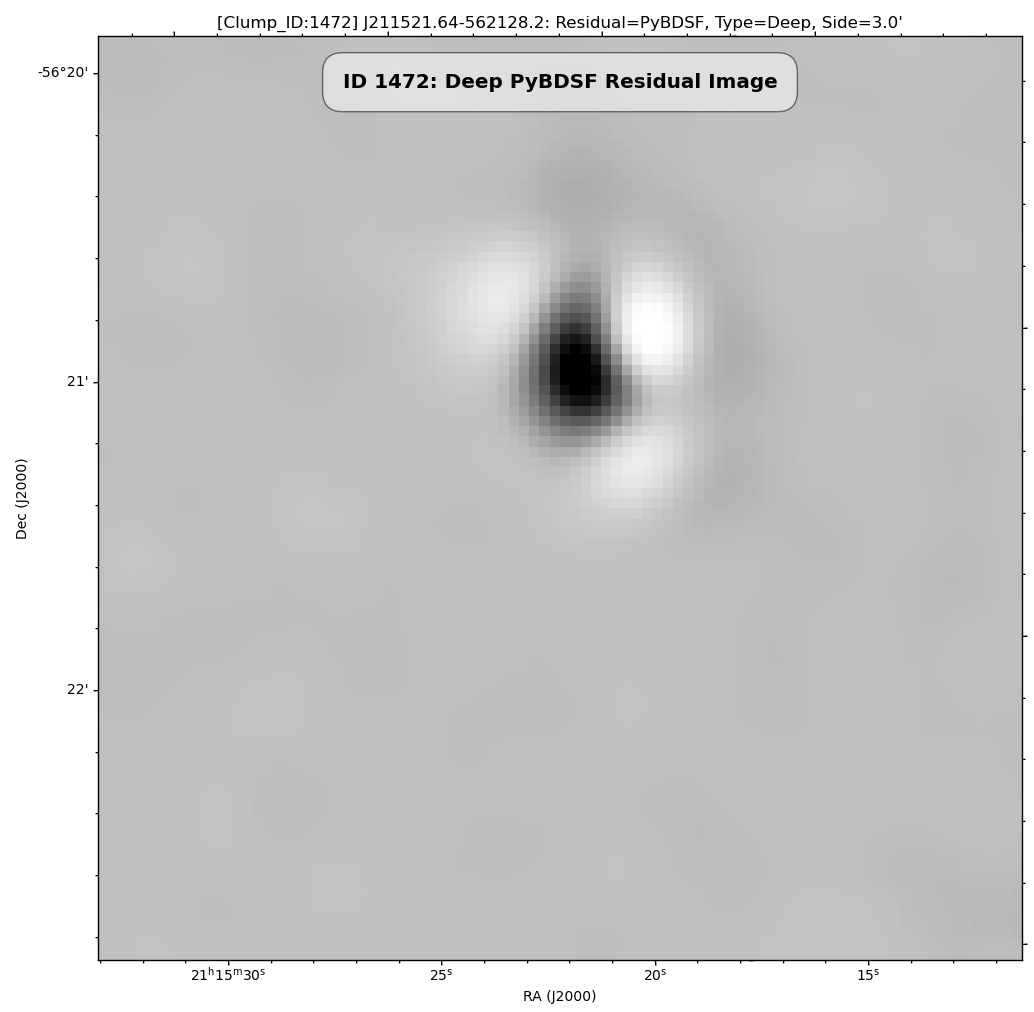
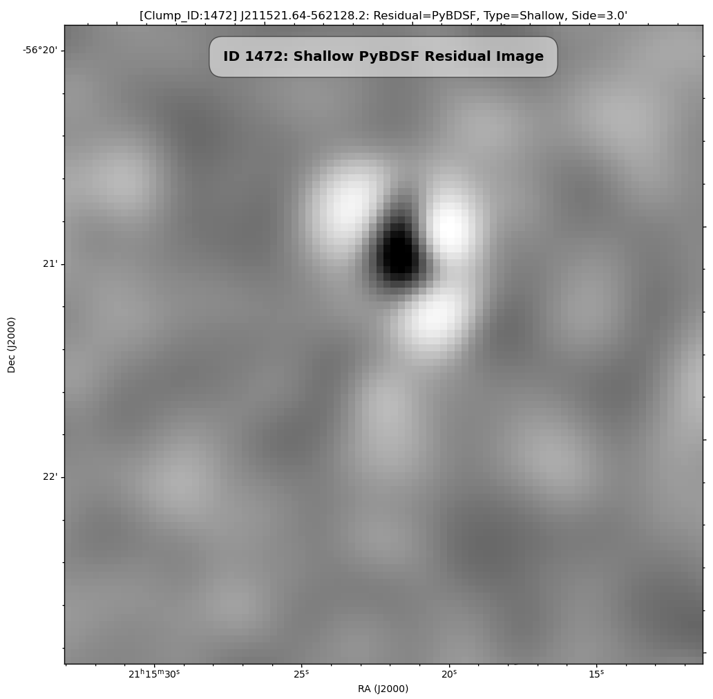
Figure 12: PyBDSF clump_id 1472 $\mathcal{D}$ (top) and $\mathcal{S}$ (bottom) $1.69^{\prime}\times 1.69^{\prime}$ residual-image cutouts for real (EMU) sources. PyBDSF fits the core of the source shown in Figure 10a, while leaving out the diffuse emission (i.e., it over-subtracts), in both $\mathcal{D}$ and $\mathcal{S}$ images. This contributes to the $\mathcal{C_{DS}}$ S/N $\sim$ 152 bin (Figure 4a).

3.6.4 Noise Spike Detection

All of the SFs detect noise spikes at low S/N that are impossible to distinguish from true sources, e.g., Figure 13. Such cases must be handled statistically, with a knowledge of the reliability of a given SF as a function of S/N, in order to treat the properties of such catalogues robustly. As image (and survey) sizes become larger, such false sources will be detected in higher numbers, as the number simply scales with the number of resolution elements sampled (Hopkins et al., 2002).

Figure 13: Noise Spike Detection Infographic: CMP $\mathcal{D}$-image (a), EMU PyBDSF $\mathcal{D}$-residual-image (b), and EMU $\mathcal{D}$-image (/w ProFound residual-image inset) (c) cutout examples of noise spike detection. In example (a) (from the $\mbox{S/N}\sim 12.4\pm 1.4$ bin of $\mathcal{R_{D}}$, Figure 4b), the detections within this clump are anomalous, as there is no injected source. In example (b), Aegean and PyBDSF detect a $\mathcal{D}$ source (match_id 1549) here, although visually this object is consistent with a noise spike. With no corresponding $\mathcal{S}$ detection, such results contribute to the inferred $\mathcal{C_{D}}$ at low S/N (Figure 5a). Example (c): At first glance, match_id 9535 appears to be part of a faint ring structure, something for which ProFound is uniquely suited. The size of the emission is on the order of common EMU’s beam size ($18^{\prime\prime}$), making it consistent with either a noise spike or a faint compact source.

3.6.5 Bright, High S/N Sources Missed

Figure 14 shows an EXT $\mathcal{D}$-image example of a bright source (clump_id 4142 /w $\mbox{S/N}\sim 226$) near a fainter source to the south (clump_id 4141 /w $\mbox{S/N}\sim 19$), representing a high $\mathcal{C_{D}}$ $\mbox{S/N}\sim 220$ bin (Figure 4g) failure mode. All SFs detected the bright source, except for Caesar. Only Selavy detects the fainter source.

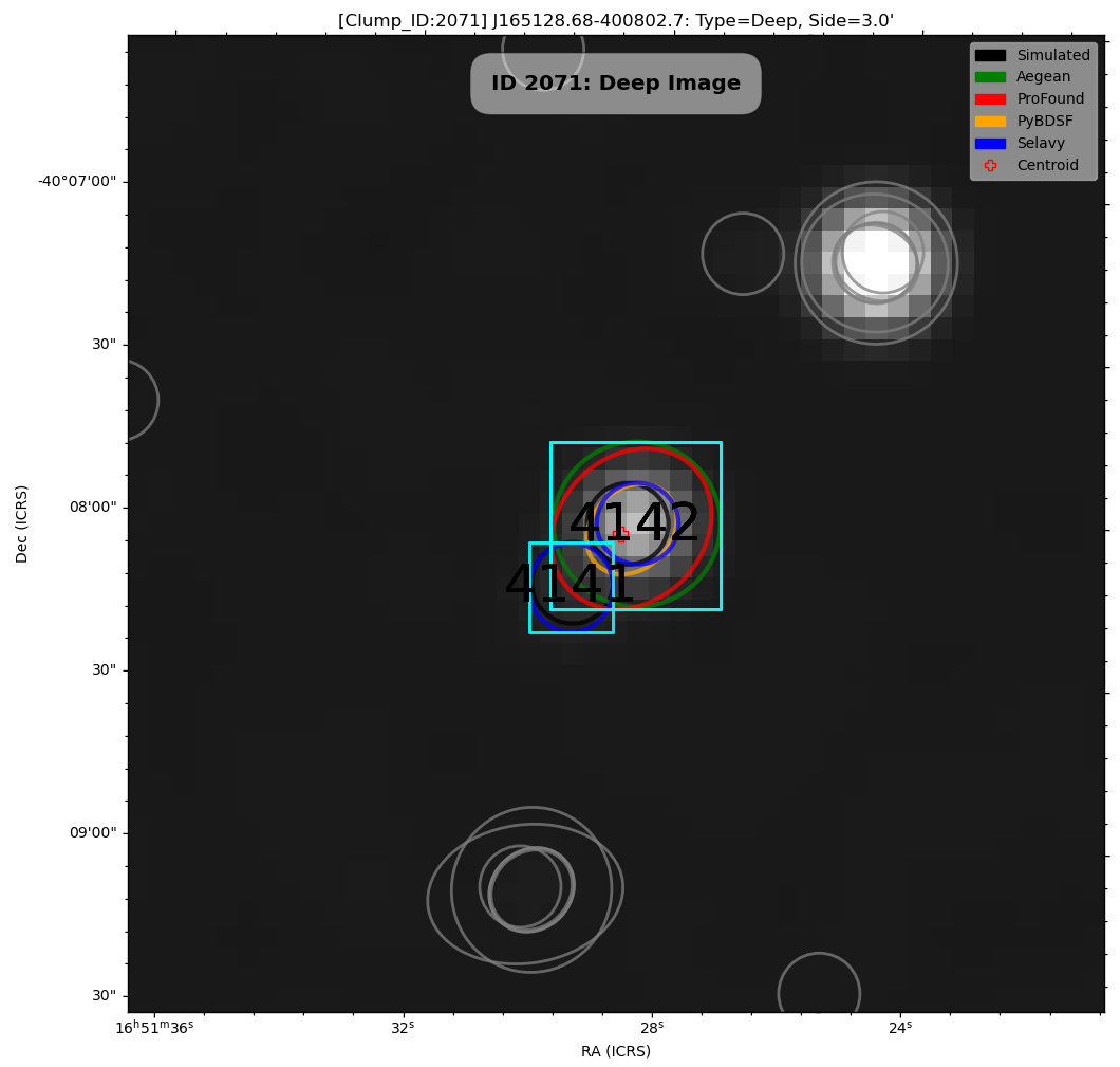
Figure 14: $3^{\prime}\times 3^{\prime}$ image cutout of clump_id 2071 of the EXT $\mathcal{D}$-image. All SFs detected the injected source ($\mbox{S/N}\sim 226$) at match_id 4142, except for Caesar. Only Selavy detects the adjacent fainter source, match_id 4141, where $(\mbox{S/N})_{injected}\sim 19$. This information was extracted from the $\mathcal{C_{D}}$ $\mbox{S/N}\sim 220\pm 25$ bin of Figure 4g.

Even at the brightest end, sources can be missed by SFs. An example is Selavy failing to detect one of two injected sources in the $C_{D}$ $\mbox{S/N}\sim 4130\pm 460$ bin (Figure 4g): i.e., it fails to detect the first of $\mbox{(S/N})_{\mathcal{D}}^{\mbox{\tiny Injected}}$ $\sim$ 4320 and 4540 at clump_ids 2363 and 270, respectively. Oddly, Selavy does detect this source in the $\mathcal{S}$-image (matching $\mbox{(S/N})_{\mathcal{S}}^{\mbox{\tiny Injected}}\sim 1365$ with $\sim 1364$), suggesting the failure in the $\mathcal{D}$-image may be related to its background estimation in this case.

3.6.6 Simulated Anomalies

Figure 15 shows an example of injected sources spanning $0.28<\mbox{S/N}<80$ in clump_id 50, with details in Table 8, for our EXT $\mathcal{D}$-image. This is an informative clump, as it encapsulates a moderately rich environment in which to explore detection anomalies. The $\mathcal{D}$-residual-image cutouts from the four SFs that make detections are shown in Figure 16. All SFs make detections in the $\mathcal{D}$ and $\mathcal{S}$ images, except for Selavy which only finds sources in the $\mathcal{S}$-image. This may arise from Selavy’s underlying Duchamp-style thresholding (Whiting, 2012).

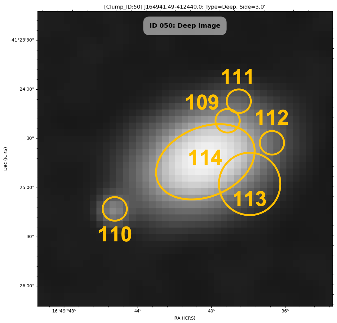
Figure 15: $3^{\prime}\times 3^{\prime}$ cutout of clump_id 50 of the EXT $\mathcal{D}$-image. The orange ellipses indicate injected sources, summarised in Table 8. The associated SF detections are shown in Figure 16. These sources span $0.28<\mbox{S/N}<80$ in $\mathcal{C_{D}}$ (Figure 4h).

Table 8: Summary of injected EXT-sources in Figure 15. The Detected column indicates if at least one SF has detected an injected source.

$\mathcal{C_{D}}$ S/N Bins	Injected	RMS	match_id	Detected
(Fig. 4g)	S/N	(mJy/beam)	(Fig. 15)	(Fig. 16)
$0.318\pm 0.036$	0.287	0.130	113	False
$0.784\pm 0.088$	0.810	0.129	112	False
$2.42\pm 0.27$	2.30	0.115	109	False
$3.80\pm 0.43$	4.01	0.114	111	False
$36.2\pm 4.0$	37.4	0.0949	110	True
$71.2\pm 8.0$	69.2	0.114	114	True

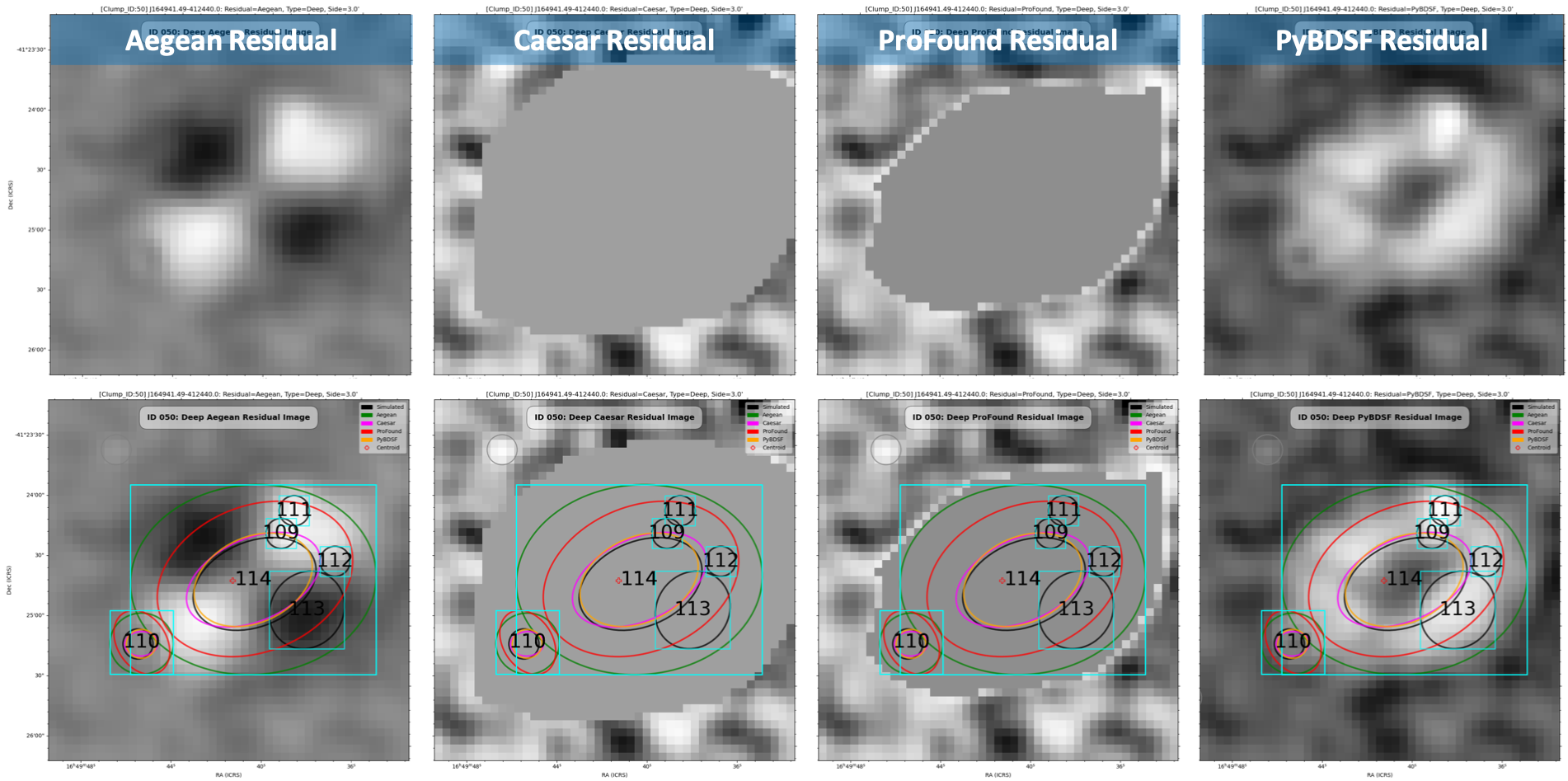
Figure 16: $2.51^{\prime}\times 2.51^{\prime}$ cutout, without (top) and with (bottom) annotations, of clump_id 50 of the EXT $\mathcal{D}$-image. The corresponding injected sources are shown in Figure 15. Aegean (green), Caesar (cyan), ProFound (red), and PyBDSF (gold) make $\mathcal{D}$ and $\mathcal{S}$ detections at match_ids 110 and 114 only, except for Selavy which only finds them in the $\mathcal{S}$-image (not shown).

For simulated images, based on the flux ratios in Figure 6, Selavy appears to produce a catalogue with an effective detection threshold of $5\sigma$, regardless of its RMS parameter setting. Recalling that the EXT image contains extended-component elements with a maximum peak flux density of $1\,$mJy, as opposed to $1\,$Jy for its compact-component elements (§ 3.1), this suggests the issue may be related to the extended low surface brightness emission around such objects. There is a roughly 10% degradation in $\mathcal{C_{D}}$, comparing the results for CMP sources alone (Figure 4a) to the EXT sources (Figure 4g). While this degradation approximates the fraction of injected EXT sources, not all the missed sources are extended. It does seem likely, though, that it is the EXT sources that contribute disproportionately to the shortfall in $\mathcal{C_{D}}$.

Comparing $\mathcal{C_{S}}$ (Figure 4i) and $\mathcal{C_{D}}$ (Figure 4g) for EXT sources, the distributions are consistent with the addition of the 5$\sigma$ noise level (shifting the S/N axis by 5 units), for most SFs (e.g., the value of $\mathcal{C_{S}}$ at $\mbox{S/N}=10$ is similar to the value of $\mathcal{C_{D}}$ at $\mbox{S/N}=5$). Selavy shows a different behaviour in that its performance in the $\mathcal{S}$-image appears to be better than in the $\mathcal{D}$-image. At the lowest S/N end this is related to faint low surface brightness objects lying below the detection threshold in the $\mathcal{S}$-image, and not contributing to the $\mathcal{C_{S}}$ and $\mathcal{C_{D}}$ distributions. At moderate and high S/N, though, the reason for the difference is less clear. It may be that faint extended emission around bright objects misleads Selavy in the $\mathcal{D}$-image, by being pushed below the noise level in the $\mathcal{S}$-image it makes the bright central region of those sources more easily detectable.

It is clear from the details in Table 8 that the sources not explicitly detected by any SF are at low S/N. Their detection is also confounded by the overlap with the brightest source (match_id 114). Aegean and ProFound have handled this by extending the size of the detection associated with match_id 114, influenced by the additional low S/N emission. This leads to over-estimation by Aegean of the source flux density and mischaracterisation of its orientation (evidenced by the oversubtraction in its residual). ProFound simply associates all the flux with the single object, which leads to a flux density overestimate compared to the input flux density of match_id 114. Caesar searches for blobs nested inside large islands, allowing a more accurate characterisation of such overlapping sources. These residual statistics are demonstrated in Table 3. Here the residual statistic values are significantly lower for ProFound and Caesar than the other SFs.

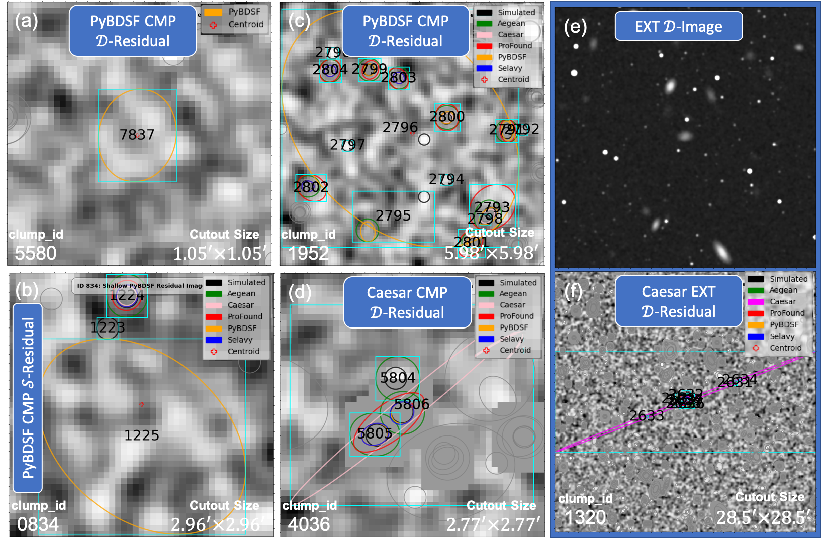
Figure 17: Oversized Components Infographic: CMP PyBDSF $\mathcal{D}$ ((a) and (c)) and $\mathcal{S}$ (b) residual-image, Caesar $\mathcal{D}$ (d) residual-image, and EXT $\mathcal{D}$-image (e) and Caesar $\mathcal{D}$-residual-image (f) cutout examples of oversized components. Example (a) (from the $\mbox{S/N}\sim 12.4\pm 1.4$ bin of $\mathcal{R_{D}}$, Figure 4b) is a spurious detection as there is no injected source. In example (b) (from the $\mbox{S/N}\sim 12.4\pm 1.4$ bin of $\mathcal{R_{D}}$, Figure 4b), the detection by PyBDSF at match_id 1225 is spurious, as there is no injected source at this location. In example (c), the large-footprint detection by PyBDSF at match_id 2796 demonstrates one of its most frequent failure modes. Its flux density is 1.84 mJy, as compared to 0.0798 mJy for the injected source. In example (d) (from the $\mbox{S/N}\sim 20.7\pm 1.4$ bin of $\mathcal{C_{DS}}$, Figure 4a), Caesar’s Gaussian fit at match_id 5806 extends well beyond its island. Its flux density estimate is 2.18 mJy compared to 0.14 mJy for the injected source. (For clump_ids 5804 and 5805 the injected flux densities are 0.07 mJy and 0.12 mJy, respectively.) In examples (e–f) (from the $\mbox{S/N}\sim 259\pm 39$ bin of $\mathcal{C_{S}}$, Figure 4a), Caesar overestimates the flux density at match_id 2639, with $18\,$mJy, compared to $0.074\,$mJy for the injected source. Its respective semi-major and semi-minor axes are $920^{\prime\prime}$ and $11^{\prime\prime}$, compared to $20^{\prime\prime}$ and $10^{\prime\prime}$ for the injected source.

3.6.7 Oversized Components

For CMP sources, PyBDSF sees the largest number of false detections within the $\mathcal{R_{D}}$ $\mbox{S/N}\sim 12$ bin of Figure 4b (a false/true ratio of 86/522). Figure 17a shows an example of one of these, illustrating a major failure mode for PyBDSF. It tends to overestimate source sizes due to inclusion of nearby noise spikes. At low or modest S/N even small noise fluctuations can lead it to expand its island in fitting to the source. Figure 17b shows another example, here with an excessively large size ($\sim 67^{\prime\prime}$), associated with the dip in the $\mathcal{R_{S}}$ $\mbox{S/N}\sim 12$ bin of Figure 4d. Figure 17c shows an example where a real injected source is the centre of a 10-component PyBDSF clump, spanning $\sim 156^{\prime\prime}$.

Turning to $\mathcal{R_{D}}$ (Figure 4b) and $\mathcal{R_{S}}$ (Figure 4d), at the lowest S/N levels ($\mbox{S/N}\lesssim 3$) Caesar appears to be reporting large numbers of false sources, leading to poor reliability. All of these artifacts are of the same nature as shown in Figure 17d. They spatially coincide with the injected sources, but overestimate the flux density due to fitting an extreme ellipse with artificially large major axis. A catastrophic example of this effect is found in the $\mathcal{C_{S}}$ $\mbox{S/N}\sim 260$ bin of Figure 4g for EXT sources, shown in Figure 17 (e–f).

3.6.8 Oddities

There are some oddities that occur less frequently, such as Caesar underestimating flux (Figure 10d) or Selavy detecting bright sources in the $\mathcal{S}$, but not $\mathcal{D}$ (Figure 16), images, where all the other SFs succeed. In the former case, it is a deblending issue with mixtures of low and high S/N sources in close proximity. The latter case is not easily explained, but may be related to poor background estimation.

3.7 Diffuse Emission Case Study

We now consider an example of a source with a combination of complex structures. The system is introduced in Figure 18, with bright compact features labelled (a) through (e), and diffuse extended emission as ($\chi$), ($\epsilon$), and ($\lambda$). We distinguish the main complex, broadly referred to herein as a bent-tail source, although the details of its nature are likely much more complex, from the bright adjacent component. This main complex is given the label B2293 (not marked in the figure, with the prefix “B” for “bent-tail”). The bright adjacent component (labelled C2294, with the prefix “C” for “compact”) is identified here as a separate clump. While the emission in C2294 seems highly likely to be related to the emission from B2293, our approach to associating detections into clumps relies on their component footprints touching or overlapping. The compact nature of C2294 leads the SFs to characterise it with ellipses that do not overlap with any ellipse in B2293, and these are consequently marked as independent clumps. The source at match_id 2667, indicated in the figure, does end up being associated with clump B2293, although it is not physically associated with the complex system (B2293+C2294). Details are given in Table 9, where we have chosen to list the MADFM as a representative statistic to characterise residuals (e.g., Riggi et al., 2019), although the other statistics are still computed, and give similar results. This complex of emission provides a good illustration of how the different SFs perform with multiple overlapping, extended and diffuse structures.

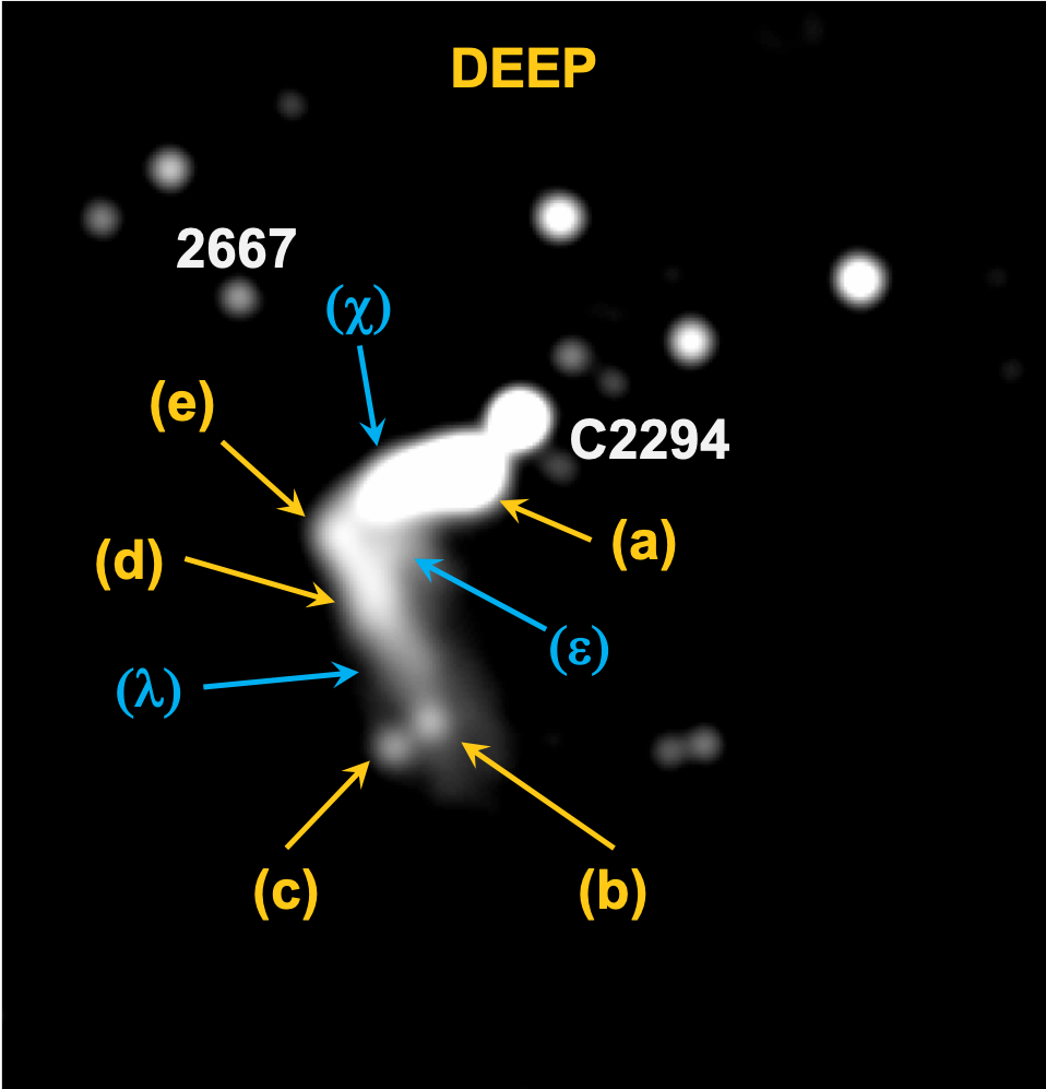
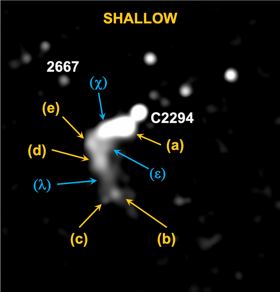
Figure 18: $\mathcal{D}$ (top) and $\mathcal{S}$ (bottom) real image (EMU) cutouts of clump_id 2293 (see also Figure 19 and Table 9). The elements of the main clump (referred to as B2293) are labelled (a) through (e) for bright compact emission, and ($\chi$), ($\epsilon$), and ($\lambda$) for diffuse emission. Also shown is match_id 2667, which is identified as part of this clump, although not physically associated. While highly likely to be related to the emission from B2293, the clump labelled C2294 is separated in our analysis. Its compact nature leads the SFs to characterise it with ellipses that do not overlap with any ellipse in B2293, resulting in these being labelled as independent clumps.

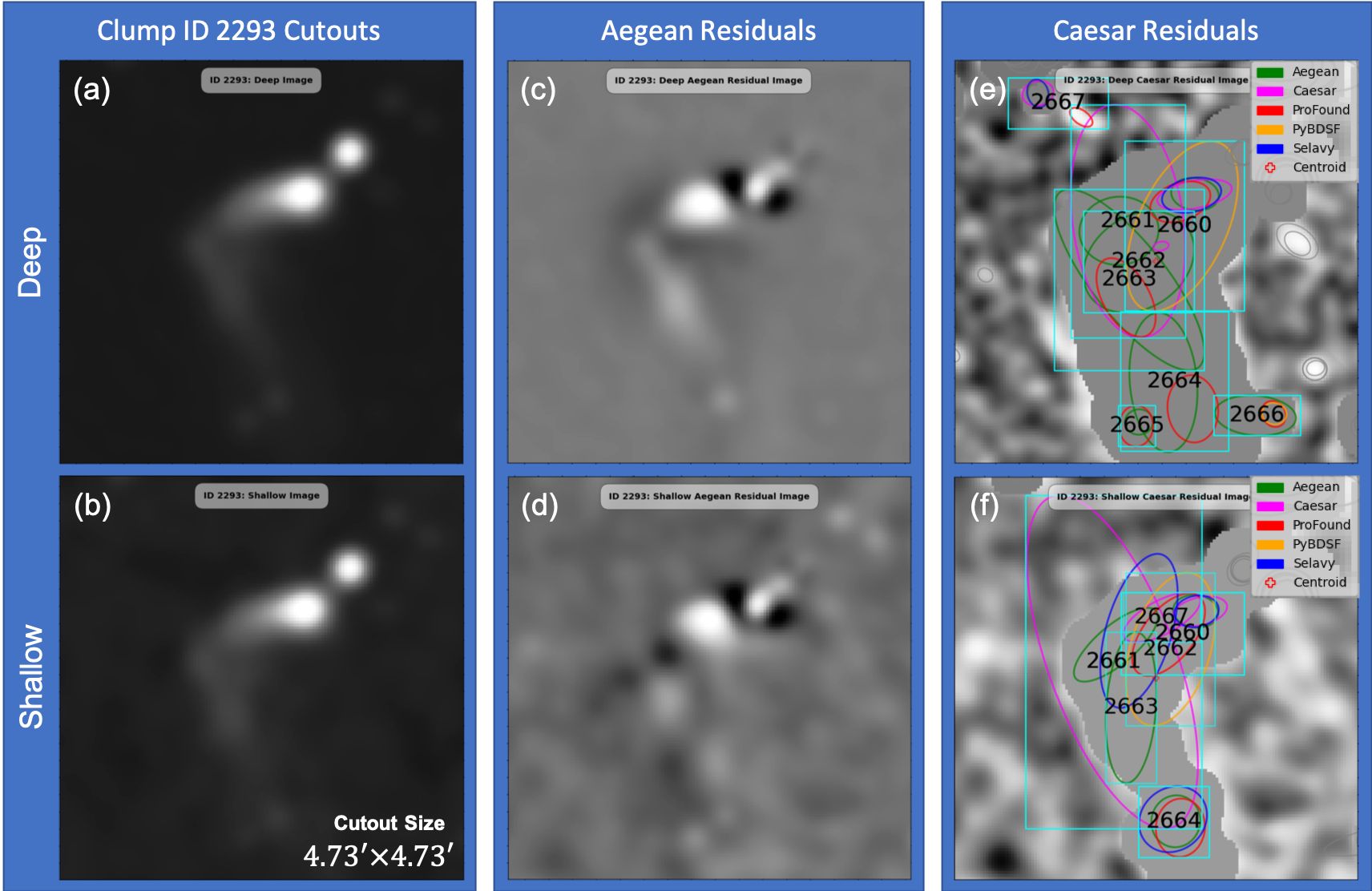
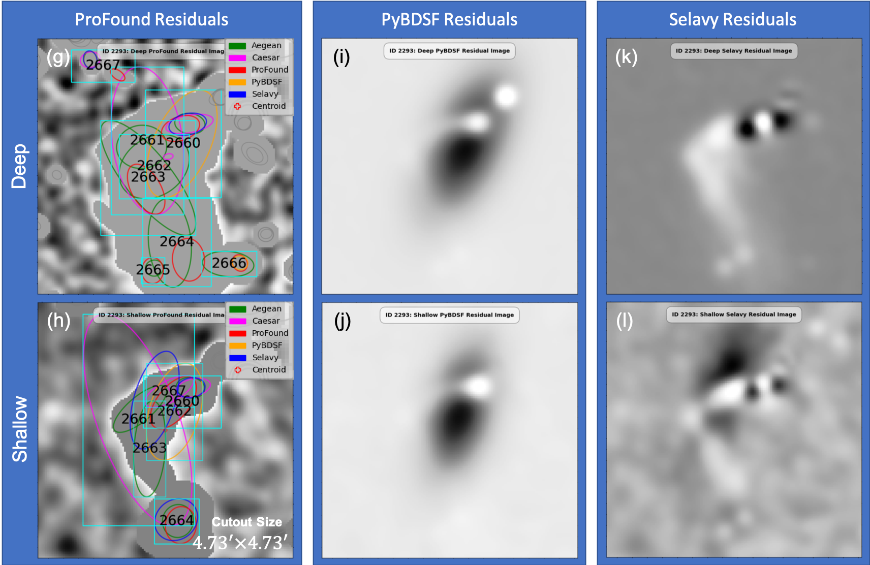
Figure 19: $4.73^{\prime}\times 4.73^{\prime}$ $\mathcal{D}$ and $\mathcal{S}$ real-image (a–b), and Aegean (c–d), Caesar (e–f), ProFound (g–h), PyBDSF (i–j), and Caesar (k–l) residual-image cutouts for clump_id 2293 of the B2293+C2294 bent-tail system. Only the Caesar and ProFound cutouts are annotated with match_id information (Table 9) for clarity.

Table 9: Cluster table information for clump_ids 2293 (upper partition) and 2294 (lower partition). The cutouts shown in Figure 19 are for the upper partition. The source component footprint parameters, $a$, $b$, and $\theta$, correspond to the major axis, minor axis, and position angle, respectively. The S/N is calculated using the noise in the $\mathcal{S}$-image, estimated using bane. The MADFMs are computed within the source component footprints and normalised with respect to their areas for the residual images. The values for ProFound are its flux-weighted estimates (Paper I).

Match	SF	Image	RA	Dec	$a$	$b$	$\theta$	$S$	S/N	MADFM
ID		Depth	(∘)	(∘)	(′′)	(′′)	(∘)	(mJy)		$\mbox{mJy}/(\prime^{2}\mbox{beam})$
2660	Aegean	Deep	320.614	-56.011	33.75	22.85	82.447	51.0417	105.4360	2.4513$\times 10^{3}\;\;$
2660	Aegean	Shallow	320.614	-56.012	31.88	22.87	82.612	49.0351	101.2908	1.0319$\times 10^{2}\;\;$
2660	Caesar	Deep	320.614	-56.011	53.35	19.46	-79.362	52.5567	108.5653	5.5643$\times 10^{4}\;\;$
2660	Caesar	Shallow	320.612	-56.012	39.18	19.61	-76.716	37.7645	79.6115	5.0744$\times 10^{3}\;\;$
2660	ProFound	Deep	320.619	-56.013	43.97	26.57	109.235	69.8364	136.9028	6.1224$\times 10^{5}\;\;$
2660	ProFound	Shallow	320.624	-56.016	68.82	35.74	141.154	85.2258	159.2764	5.6682$\times 10^{3}\;\;$
2660	PyBDSF	Deep	320.619	-56.017	128.89	62.74	155.166	126.1139	246.0558	1.2288$\times 10^{2}\;\;$
2660	Selavy	Deep	320.615	-56.012	42.40	23.71	102.080	61.3140	125.3935	2.6793$\times 10^{3}\;\;$
2660	Selavy	Shallow	320.613	-56.012	31.47	22.05	100.170	46.5150	97.0618	1.0414$\times 10^{2}\;\;$
2661	Aegean	Deep	320.642	-56.017	55.90	48.05	-84.490	17.5477	37.3929	2.4513$\times 10^{3}\;\;$
2661	Aegean	Shallow	320.642	-56.017	73.95	27.27	-49.783	17.7016	38.2606	1.0319$\times 10^{2}\;\;$
2661	Caesar	Deep	320.638	-56.016	165.70	78.08	8.087	73.9215	151.3647	5.5643$\times 10^{4}\;\;$
2661	Caesar	Shallow	320.644	-56.020	248.30	90.18	20.210	90.2743	195.1955	5.0744$\times 10^{3}\;\;$
2661	Selavy	Shallow	320.634	-56.014	112.44	46.23	163.650	60.2680	118.3390	1.0414$\times 10^{2}\;\;$
2662	Aegean	Deep	320.636	-56.024	83.96	64.66	-55.037	17.7797	34.2307	2.4513$\times 10^{3}\;\;$
2662	Caesar	Deep	320.627	-56.021	10.93	6.24	-78.426	0.1349	0.2410	5.5643$\times 10^{4}\;\;$
2662	PyBDSF	Shallow	320.624	-56.018	111.50	56.04	162.988	156.9845	293.7207	1.7932$\times 10^{2}\;\;$
2663	Aegean	Deep	320.639	-56.027	157.56	52.04	38.318	3.2044	6.4656	2.4513$\times 10^{3}\;\;$
2663	Aegean	Shallow	320.639	-56.029	106.85	35.06	-4.002	21.3041	44.3798	1.0319$\times 10^{2}\;\;$
2663	ProFound	Deep	320.641	-56.030	61.32	32.77	29.961	21.4079	46.5896	6.1224$\times 10^{5}\;\;$
2664	Aegean	Deep	320.630	-56.048	98.68	47.38	5.068	14.5981	43.9117	2.4513$\times 10^{3}\;\;$
2664	Aegean	Shallow	320.627	-56.052	36.73	34.34	-12.335	6.0130	21.4578	1.0319$\times 10^{2}\;\;$
2664	ProFound	Deep	320.621	-56.053	47.60	35.67	5.535	7.5893	28.1344	6.1224$\times 10^{5}\;\;$
2664	ProFound	Shallow	320.625	-56.054	41.23	34.49	173.862	10.5205	39.3395	5.6682$\times 10^{3}\;\;$
2664	Selavy	Shallow	320.628	-56.052	50.22	43.97	128.550	10.8400	37.7821	1.0414$\times 10^{2}\;\;$
2665	Aegean	Deep	320.640	-56.055	19.85	17.86	-84.110	0.8030	3.3544	2.4513$\times 10^{3}\;\;$
2665	ProFound	Deep	320.641	-56.056	29.00	23.98	178.631	2.4034	10.3152	6.1224$\times 10^{5}\;\;$
2666	Aegean	Deep	320.599	-56.056	57.28	28.06	85.426	0.9795	4.0272	2.4513$\times 10^{3}\;\;$
2666	ProFound	Deep	320.593	-56.056	19.18	16.12	31.535	0.3273	1.3524	6.1224$\times 10^{5}\;\;$
2666	PyBDSF	Deep	320.593	-56.056	17.38	15.17	80.152	0.1721	0.7110	1.2288$\times 10^{2}\;\;$
2667	Aegean	Deep	320.666	-55.989	18.68	14.42	2.981	0.1361	0.5255	2.4513$\times 10^{3}\;\;$
2667	Caesar	Deep	320.666	-55.989	22.20	17.07	-76.756	0.1552	0.5994	5.5643$\times 10^{4}\;\;$
2667	Caesar	Shallow	320.626	-56.012	59.98	23.76	-62.079	22.7529	42.1717	5.0744$\times 10^{3}\;\;$
2667	ProFound	Deep	320.651	-55.995	18.49	9.79	54.245	0.1416	0.3971	6.1224$\times 10^{5}\;\;$
2667	PyBDSF	Deep	320.666	-55.989	19.98	14.83	7.938	0.1606	0.6202	1.2288$\times 10^{2}\;\;$
2667	Selavy	Deep	320.666	-55.989	19.92	14.88	12.690	0.1610	0.6216	2.6793$\times 10^{3}\;\;$
2668	Aegean	Deep	320.595	-56.004	18.82	18.40	-87.136	20.9655	53.8435	1.3433
2668	Aegean	Shallow	320.595	-56.004	18.65	18.41	87.954	20.9354	53.7664	1.1211
2668	Caesar	Deep	320.595	-56.004	27.80	16.61	-68.410	20.6564	53.0499	0.0000
2668	Caesar	Shallow	320.595	-56.004	25.56	20.72	-48.870	21.5519	55.3497	0.0000
2668	ProFound	Deep	320.596	-56.004	16.68	16.01	141.799	21.8717	55.5098	0.0000
2668	ProFound	Shallow	320.596	-56.004	16.05	14.91	132.551	21.5683	54.7398	0.0000
2668	PyBDSF	Shallow	320.595	-56.004	19.06	18.04	123.511	20.8894	53.6482	7.8357
2668	Selavy	Deep	320.595	-56.004	18.53	17.57	99.270	19.9640	51.2715	1.1786
2668	Selavy	Shallow	320.595	-56.004	19.04	18.21	123.250	21.3080	54.7232	4.7455$\times 10^{-1}$

C2294 corresponds to match_id 2668 of clump_id 2294. The clump information for this object is given in the lower partition of Table 9. We have not included the cutout images for this system (whose SF components are greyed out in Figure 19e–h), as, in general, we are focusing our attention on the complex source (B2293). The following discussion arises from consideration of the detections and residuals shown in Figures 18 and 19, and Table 9, with explicit reference where clarity is required.

The interpretation of $(\varepsilon)$ and $(\lambda)$ as purely diffuse emission is subjective, based only on their appearance in this radio image, without consideration of possible optical or infrared counterparts. Similarly, the component labelled $(\chi)$ appears subjectively to be a bright extension from $(a)$. The annotations $(a)$ through $(e)$ are likewise subjectively identified as compact components. This choice is adequate for the current discussion given that this is the same information being used by the SFs.

Aegean cleanly identifies C2294 (match_id 2668) and the component at $(a)$ (match_id 2660) in the $\mathcal{D}$ and $\mathcal{S}$ images. While it identifies several additional components (match_ids 2661, 2662, 2663, 2664, 2665, 2666) to characterise the complex of compact and diffuse emission, these poorly model the emission itself as evidenced in the residuals, for both $\mathcal{D}$ and $\mathcal{S}$ images. It is clear from the annotations, too, that the components identified in the $\mathcal{S}$-image (match_ids 2661, 2663, 2664 only) are markedly different from their counterparts in the $\mathcal{D}$-image. The component sizes tend to overestimate the extent of the true emission and are often poorly aligned with the structure. Such mismatches, as discussed above, lead to a reduction in $\mathcal{C_{DS}}$ and $\mathcal{R_{DS}}$. For these complex structures, Aegean generally identifies source positions biased towards flux-weighted centers, with fitted component sizes compensating for the total flux within. This affects the position and size accuracy of the region it is trying to characterise.

Caesar robustly identifies C2294 (match_id 2668) and $(a)$ (match_id 2660) in the $\mathcal{D}$ and $\mathcal{S}$ images. In the $\mathcal{D}$-image, $(\chi)$ is incorporated into its estimate of the source $(a)$. In the $\mathcal{S}$-image, it resolves the two separately into $(a)$ and $(\chi)$ (match_id 2667). Recall that Caesar is designed to be sensitive to diffuse emission (Riggi et al., 2016), which is evident in the extent of its residual-image footprint (representing the parent-blob, Figure 19). It correctly characterises the extent and overall shape of the emission. The individual components (child-blobs) are determined in its second iteration. Refinement of the parameters for that step may lead to improvements in the way the various components are characterised. This step was not deemed to be practical for the current implementation of Hydra, and it is also unclear whether fine-tuning for such an individual source would have unintended effects for rest of the image. This is an aspect that can be explored in future developments of the tool. Having acknowledged this point, in this implementation Caesar does poorly in terms of characterising most of the components, with the exception of detecting $(\varepsilon)$ in the $\mathcal{D}$-image (match_id 2662 with S/N $\sim$ $0.2\,$mJy). It attempts to fit everything by a single component (match_id 2661), both in the $\mathcal{D}$ ($a\sim 166^{\prime\prime}$, $b\sim 78.1^{\prime\prime}$, and $\theta\sim 8.09^{\circ}$ with $S\sim 73.9\,$mJy) and $\mathcal{S}$ ($a\sim 248^{\prime\prime}$, $b\sim 90.2^{\prime\prime}$, and $\theta\sim 20.2^{\circ}$ with $S\sim 90.3\,$mJy) images. Here $a$, $b$ and $\theta$ are the fitted major and minor axes and position angle respectively. These correspond to S/N bins 152 and 181, respectively. The mismatch between these components in the $\mathcal{D}$ and $\mathcal{S}$ images contribute to a degradation in $\mathcal{C_{DS}}$ (Figure 5a).

ProFound does a good job of characterising the features of B2293+C2294 in the $\mathcal{D}$-image, but less so in the $\mathcal{S}$-image. As with Caesar, ProFound accurately characterises the extent and overall shape of the emission in general, as seen in the residual images for both $\mathcal{D}$ and $\mathcal{S}$. It tends to merge brighter peaks with adjacent diffuse emission. The combinations $(a)+(\chi)$, $(e)+(\varepsilon)+(d)+(\lambda)$, $(b)$, and $(c)$ are identified in match_ids 2660, 2663, 2664, and 2665, respectively. This is consistent with ProFound’s design, identifying diffuse islands and characterising them through such flux-weighted components. In the $\mathcal{S}$-image, ProFound does not do as well because much of the diffuse emission is washed out. This becomes clear by comparing the $\mathcal{D}$ and $\mathcal{S}$ residual images in Figure 19 through the reduction in its island size (this is also apparent with Caesar, but to a lesser degree). In the $\mathcal{S}$-image ProFound breaks B2293 into two main components, everything along the chain from $(a)-(\lambda)$ in match_id 2660, and $(b)+(c)$ in match_id 2664. This again results in a mismatch between the components in the $\mathcal{D}$ and $\mathcal{S}$ images.

PyBDSF does not perform well for extended sources with diffuse emission. It tends to merge things together and attempt to fit complex regions with a single Gaussian. In the $\mathcal{D}$-image it merges the B2294+C2294 system into one component (match_id 2660), whereas in the $\mathcal{S}$-image they are separated into two components, B2263 (match_id 2662) and C2294 (match_id 2668). Clearly it is representing the system largely as a single island in the $\mathcal{D}$-image, due to the presence of the extended diffuse emission. In the $\mathcal{S}$-image it is resolved into two, as the diffuse emission linking B2294 and C2294 is masked by the higher noise level. With our settings (Paper I), PyBDSF uses the number of peaks found within the island as its initial guess for the number of Gaussians to fit, iteratively reducing them until a good fit is achieved (Mohan & Rafferty, 2015). Here, presumably, it is the diffuse emission that is affecting the fit quality, as can be seen in the residual images. This is also consistent with the failure modes seen in our simulated point source image, (Figures 17a–c). Figure 17c may be a good analogy, where PyBDSF fits a single component to a large region encompassing multiple injected sources presumably influenced also by peaks in the background noise, mimicking the diffuse emission in this case.

Selavy accurately characterises C2294 (match_id 2668) in the $\mathcal{D}$ and $\mathcal{S}$ images, but does poorly with B2294. B2294 is characterised by a single component in the $\mathcal{D}$-image, at match_id 2660, and by three components in the $\mathcal{S}$-image, at match_ids 2660, 2661, and 2664. It appropriately characterises $(a)+(\chi)$ in the $\mathcal{D}$ and $(a)$ in the $\mathcal{S}$, at match_id 2660. This is not unexpected, given the diffuse emission is reduced in the latter. Perhaps surprisingly, though, it misses the remainder of the emission beyond $(\chi)$ in the $\mathcal{D}$-image. In the $\mathcal{S}$-image it detects two components here, linking the emission spanning $(\chi)-(\lambda)$ (match_id 2661) and $(b)+(c)$ (match_id 2664). Selavy’s approach also includes a stage of rejecting poorly fit components (Whiting & Humphreys, 2012), and that may be the issue with the lack of components reported for the emission in the $\mathcal{D}$-image. This may have been slightly more successful in the $\mathcal{S}$-image (due to a reduction in the diffuse emission). This contributes to a reduction in $\mathcal{R_{DS}}$ (Figure 5b), as the $\mathcal{S}$ detection at match_id 2661 has no $\mathcal{D}$ counterpart, seen in the degradation in the S/N $\sim$ 125 bin. This effect occurs elsewhere at similarly high S/N from other sources.

3.8 Discussion

The Hydra software was used to compare the Aegean, Caesar, ProFound, PyBDSF, and Selavy SFs by first minimising the FDR based on a 90% PRD cutoff, through Typhon. Aegean, PyBDSF, and Selavy RMS box parameters were $\mu$-optimised prior to the main run. The process was done for both $\mathcal{D}$ and $\mathcal{S}$ images for $2^{\circ}\times 2^{\circ}$ CMP, EXT, and real (EMU pilot) images.

Figure 20: Diffuse Emission Case Study Summary: Summary of bent-tail system (B2293+C2294) diffuse emission case study (see § 3.7, Figures 18 and 19, and Table 9).

The RMS box optimisation produces a $\mathcal{S}$-to-$\mathcal{D}$ noise ratio of 5 for all images (Table 4), validating the routine. In addition, the baseline statistics show that the CMP source distribution is closer to the real (EMU) image than the EXT results. This is also reflected in the $\mathcal{C_{DS}}$ and $\mathcal{R_{DS}}$ plots, for CMP (Figure 4 (e-f)) and EXT (Figure 4 (k-l)) sources, when compared with the real image (Figure 5). For the simulated $\mathcal{D/S}$-images, the source detection numbers (N, Table 5) are consistent between SFs, with the exception of Selavy being unusually low. As for the real image, the number of sources detected by Aegean, Caesar, and PyBDSF are comparable, while ProFound is significantly high and Selavy is low. In the case of ProFound, this is attributed to noise, or potentially to splitting sources more than done by other SFs, whereas for Selavy it is not as clear. In general, the residual RMS values vary between SFs for each image case, whereas the residual MADFMs are consistent (Table 6). This should not be surprising as MADFM (or robust) statistics tend to miss outliers, such as bright sources (Whiting & Humphreys, 2012). This could provide a viable explanation as to Selavy’s behaviour, in this regard, as it has a tendency to miss bright sources in $\mathcal{D}$-images more often than $\mathcal{S}$-images, and we have its robust statistics flag set (Paper I). This line of reasoning is consistent with Whiting (2012), and so warrants further investigation.

In our analysis we examined major-axes, completeness, reliability, flux-ratio, and false-positive statistics (Figures 3 through 7). This was later framed in the context of residual/image cutouts case studies, in which we investigated anomalies regarding edge detection, blending/deblending, component size estimates, bright sources, diffuse emission, etc. (Figures 8 through 17): Aegean, ProFound, and PyBDSF are good at detecting sources at the edge of images, while it is more problematic for Caesar and Selavy (Figure 8). As expected, all SFs detect tightly overlapped sources as single unresolved compact sources (Figure 9), at the expense of a degradation in completeness. This is of course somewhat artificial, since with real images this situation cannot be distinguished. For $\mathcal{D}$ compact sources with diffuse emission, Aegean, ProFound, PyBDSF, and Selavy tend to flux-weight (blend) their components position and sizes (Figure 9c), characterising the core, whereas Caesar and Selavy tend to characterise (deblend) the core and diffuse halo separately (Figure 10f). For the $\mathcal{S}$ case (Figure 9d), the diffuse emission tends to be somewhat washed out, so that the SFs see predominantly compact sources (Figure 9f). Similar issues can occur for systems with a bright source among low S/N sources, contributing to a degradation in reliability (Figure 10a–b). For low S/N thresholds, all SFs are susceptible to noise spike detection, particularly so for ProFound (Figure 13c); as can be seen from its scatter, Table 7. Noise spikes also affect PyBDSF, in that it tends to collect them together, sometimes with true sources, producing oversized components (Figure 17a-c). Caesar also overestimates component size on occasion, however this is related to deblending issues (Figure 10d). It also underestimates on occasion, leading to a degradation in reliability (Figure 11).

A detailed diffuse emission case study was also explored (Figures 18 and 19) with Figure 20 summarising the results. Aegean characterises B2293 by fitting its bright spots and diffuse emission as separate components, but ignores the diffuse emission in the $\mathcal{S}$-image. Caesar detects $(a)$ in both the $\mathcal{D/S}$-images, but only identifies $(\chi)$ in the $\mathcal{S}$-image; the remaining information, is approximated by a single component. ProFound correctly characterises the shape of B2293 in the $\mathcal{D}$-image, however its components only highlight the flux-weighted centers of each segment (“island”); for the $\mathcal{S}$-image, only $(a)+(\chi)$ and $(b)$ are detected. PyBDSF treats the complex largely as a single source (it also picks up the faint isolated SW $\mathcal{D}$ source). Finally, for the $\mathcal{D}$-image, Selavy treats B2293 as a single system centered at (a), whereas it seems more successful at characterising the system in the $\mathcal{S}$-image.

4 Future Prospects

4.1 Detection Confidence

Given Hydra uses multiple SFs, it leads to the possibility of exploring cross-comparison metrics. For example, Figure 21 shows detection confidence charts, indicating coincident detections between SFs. The bar on the far left shows the number of sources detected in common between all 5 SFs. The next bar shows the numbers of sources from each SF detected in common by 4 SFs, and so on. This metric uses a “majority rules” process to help determine whether a detection is more likely to be real. If a source is only picked up by a single SF, chances are that detection is spurious (e.g., Figure 13c). The more SFs that agree on a source, the more likely it is to be real. This could be used to constrain metrics, such as completeness, reliability, flux-ratios, etc. This could be particularly useful in refining such statistics for real images, where the true underlying source population is not known a priori.

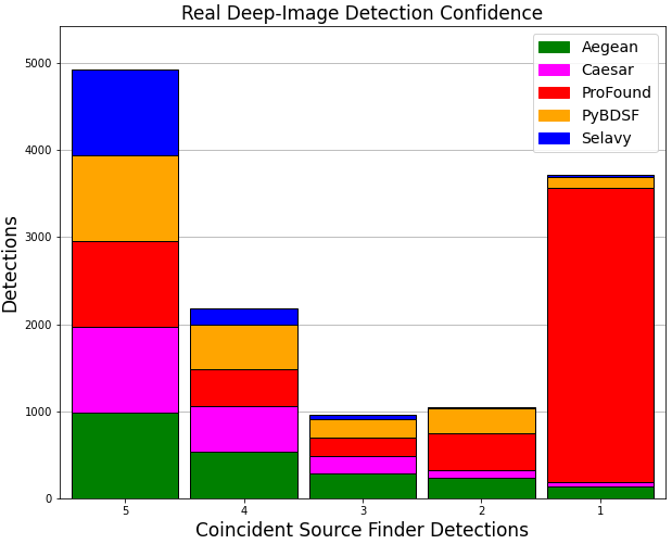
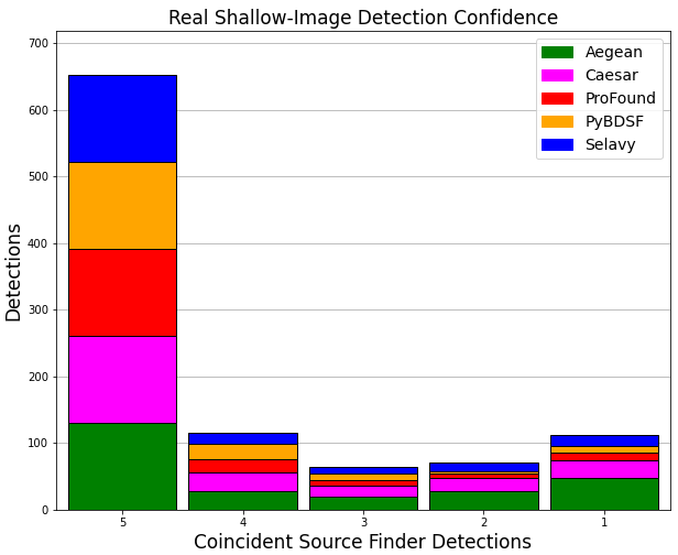
Figure 21: Real image $\mathcal{D}$ (top) and $\mathcal{S}$ (bottom) detection confidence charts. The stacked bars indicate agreement between SF detections. From left to right, 5 SFs agree, 4 SFs agree, etc.

One should be cautious, however, not to take this as ipso facto true. For example, a detection by all SFs could be a bright artifact or noise spike that mimics a source. At the other extreme one could end up excluding real sources only detected by finders well-adapted to recognising them (e.g., Figure 22). The middle ground may indicate the nature of detection, such as compact and/or extended sources with or without diffuse emission, depending on a SF’s strengths (Paper I).

Figure 22: Example of a diffuse VLASS source, uniquely detected by ProFound in a comparison study with PyBDSF (Boyce, 2020). The source was found in a $3^{\prime}\times 3^{\prime}$ region centered at J112328+064341. The cutout was extracted from a QL image tile, available at NRAO (https://science.nrao.edu), and then processed using ProFound in R Studio.

The number of possible cross-source-SF diagnostics that could be developed is substantial. Consequently we have only briefly touched on this subject here, leaving further details for future investigation.

4.2 Processing Residual Images

The existence of initially undetected sources in the residual images suggests that running a second iteration of the SFs on such residual images may potentially improve on the completeness of the delivered catalogues. This may not be practical for Caesar or ProFound, however, as they compute residuals by subtracting out all of the flux within an island; although, one could create residual images from their island components. Aegean, PyBDSF, and Selavy are perhaps more suitable, as they are Gaussian-fit based. There is, however, a challenge that arises from over-subtraction, where the initial source list includes overestimated sources (e.g., Figure 10a). Here the residuals reflect a poor initial fit, rather than true sources remaining to be detected in such a second pass.

The PyBDSF residual $\mathcal{D}$-image in Figure 16, which emphasises the undetected sources at match_ids 109, 111, 112, and 113, suggests that a second detection pass on such residual images may have merit. How best to implement such an approach remains a challenge, as it may introduce new false detections if residuals such as seen in Figure 16 with Aegean dominate, and likewise for more complex objects, containing diffuse emission.

In order to explore this further, let us consider the residual statistics of our case-study system (i.e., clump_id 2293 in Table  9) and the full EMU image (Table 3), summarized in Table 10. Three potential approaches for reprocessing residual images are:

1. process all $2^{\circ}\times 2^{\circ}$ residual images,

2. process the $2^{\circ}\times 2^{\circ}$ residual image with the best MADFM,

3. process an aggregate clump-based residual-image consisting of the best MADFM’s on a clump-by-clump basis.

Approach 1 is ruled out as being computationally impractical. To explore the other options we consider the MADFMs for CMP and EXT sources in Table 3, and real sources in Table 10.

Table 10: Residual image statistics for the full $2^{\circ}\times 2^{\circ}$ EMU pilot sample image and for clump_id 2293 drawn from it (extracted from Tables 3 and 9, respectively). The MADFMs are normalised by cutout area, and are in units of mJy arcmins^-2 beam^-1). N is the component count.

Residual Image		EMU Sample		Cutout 2293
Source	Image	$2^{\circ}\times 2^{\circ}$		$4.73^{\prime}\times 4.73^{\prime}$
Finder	Depth	N	MADFM	N	MADFM
Aegean	Deep	8,538	$2.60\!\!\times\!\!10^{-5}$	8	$2.45\!\!\times\!\!10^{-3}$
Caesar	Deep	7,838	$2.30\!\!\times\!\!10^{-5}$	4	$5.56\!\!\times\!\!10^{-4}$
ProFound	Deep	11,484	$1.90\!\!\times\!\!10^{-5}$	6	$6.10\!\!\times\!\!10^{-5}$
PyBDSF	Deep	8,292	$2.60\!\!\times\!\!10^{-5}$	3	$1.23\!\!\times\!\!10^{-2}$
Selavy	Deep	5,800	$2.70\!\!\times\!\!10^{-5}$	2	$2.68\!\!\times\!\!10^{-3}$
Aegean	Shallow	926	$1.69\!\!\times\!\!10^{-4}$	4	$1.03\!\!\times\!\!10^{-2}$
Caesar	Shallow	885	$1.66\!\!\times\!\!10^{-4}$	3	$5.07\!\!\times\!\!10^{-3}$
ProFound	Shallow	778	$1.65\!\!\times\!\!10^{-4}$	2	$5.67\!\!\times\!\!10^{-3}$
PyBDSF	Shallow	794	$1.69\!\!\times\!\!10^{-4}$	1	$5.67\!\!\times\!\!10^{-3}$
Selavy	Shallow	789	$1.69\!\!\times\!\!10^{-4}$	3	$1.04\!\!\times\!\!10^{-2}$

Given that ProFound and Caesar assign all flux in an island to a source, their residuals are zero by default at the location of sources, leading to their MADFM statistics understandably being the lowest. In order to compare them fairly to the other SFs, residual images created instead from their inferred Gaussian components would be necessary. The analysis of the complex system B2293+C2294 (Figure 18) suggests that ProFound would likely produce residual MADFMs similar to the other SFs, and potentially perform better in the case of complex extended sources with diffuse emission. Caesar would probably not fare as well, given that Hydra is not implementing its full capability for decomposing complex structures. For simplicity in the remainder of this discussion we focus on the other three SFs as potential starting places for image reprocessing.

Considering approach 2, we see that Aegean and PyBDSF have identical MADFMs in the full image. It would be easy to choose one at random, or invoke the other residual image metrics as a further discriminator. Regardless, the next challenge will be understanding and accounting for the artifacts associated with the residuals of the chosen SF. Discriminating in a second SF run between a truly overlooked component and a residual peak left by a poor first-pass subtraction seems on its face to be intractable. One approach may be not to treat each iterative pass as independent and concatenate the output catalogues, but instead to first combine the components together where they overlap in order to better reconstruct the true underlying flux distribution for each complex.

Approach 3 is perhaps more unconventional, as it draws on the aggregate of results from the different SFs. By using the cutouts with the best MADFM in each case, though, it is likely to contain fewer artifacts than the monolithic approach 2 above. Figure 23 shows a distribution of MADFMs for Aegean, PyBDSF, and Selavy. Here we only include a MADFM if it is the lowest for each clump. In other words, each clump is represented only once, and the best MADFM for it contributes to the distribution for that SF. At low MADFM values each SF appears to contribute roughly equally to the set of best residual cutouts. The corresponding aggregate residual image would be roughly a homogeneous mixture of results from the three SFs. For increasing MADFM, Selavy contributes fewer of the best residuals, followed by PyBDSF, with Aegean contributing the most at the higher values of MADFM. For our sample complex system, the aggregate would include 8 components within clump_id 2293 (which contains B2293) arising from Aegean (Table 10) and one component within clump_id 2294 (which only contains C2294) from Selavy (Table 9 bottom partition). This approach may have some merit, but clearly also adds a layer of complexity that may prove more challenging than desired.

Figure 23: Distribution of clumps with the lowest MADFM wrt Aegean, PyBDSF, and Selavy.

An alternative approach would be to first identify compact components only and produce a residual image by subtracting those, presuming that all finders perform (reasonably) well on such compact emission. This would leave a residual image consisting only of emission with more complex structure. This would then need to be processed using a SF that has demonstrated good performance with complex structures, established with another run of Hydra. This may provide the opportunity to better characterise extended emission in the vicinity of bright compact emission. If this model of multi-pass source-finding is promising, it could be further implemented iteratively, perhaps with S/N limits imposed on the initial pass(es) to first characterise and remove the bright sources, and progress to the faint population in later iterations. Either of the approaches 2 or 3 could be considered in these scenarios. The results from each pass in such approaches would then have to be incorporated with the existing cluster catalogue and appropriately tagged. While this iterative approach was one of the motivations for developing Hydra, it is clear that a considerable amount of further analysis would be required to demonstrate its value.

5 Summary and Conclusions

In Paper I we introduced the Hydra tool, and detailed its implementation, demonstrating its use with simulated image data. In this second paper of the two part series we use Hydra to characterise the performance of five commonly used SFs.

5.1 Source finder comparison and performance

Hydra was used to explore the performance of SFs through $\mathcal{C}$ and $\mathcal{R}$ statistics, and their size and flux-density measurements, as well as through targeted case studies (§ 3.6). The most significant differences appeared when encountering real sources with diffuse emission. Other frequently encountered anomalies were with sources at image edges, blending/deblending, component size errors, and poorly characterised bright sources.

In terms of characterising sources, all SFs seem to handle compact objects well. With the exception of Selavy, this generally applies to extended objects as well. In the case of compact objects with diffuse emission, Aegean, ProFound and PyBDSF tend to characterise them as point sources, whereas Caesar deblends them into cores with diffuse halos, and Selavy as cores with jet-like structures. This is all consistent with how the SFs are designed (Paper I). For more complex sources with diffuse emission, Aegean performs best at characterising their complexity through a combination of elliptical Gaussian components, with PyBDSF and Selavy overestimating component sizes, missing regions of flux, or fitting components misled by adjacent flux peaks. Caesar and ProFound characterise extended islands well, but their corresponding components are not always robust representations of the whole.

In moving from simulated to real images, we find the major distinction comes when considering diffuse sources. ProFound performs the best when it comes to complex sources with diffuse emission, characterising them as islands of flux, but without resolving them further (by design, Robotham et al., 2018). Caesar in general performs similarly, although it is not implemented optimally in the current version of Hydra. Caesar can implement different RMS and island parameters for the parent and child segments in order to improve the deblending of complex structures (Riggi et al., 2016, 2019). These are currently defined by Hydra to have the same settings, though, due to its present implementation requiring a single pair of RMS and island parameters for each SF (Paper I). In short, given the SCORPIO survey analysis by Riggi et al. (2016), Caesar is expected to outperform ProFound in terms of its deblending approach, although it may still not characterise diffuse emission to the same degree (e.g., compare Caesar and ProFound footprints in Figure 19e–f and g–h, respectively). PyBDSF and Selavy have similar performance issues. They both tend to merge together sources embedded in regions of diffuse emission, leading to different characterisations in the $\mathcal{D}$ and $\mathcal{S}$ images depending on the degree of diffuse emission present, with a corresponding impact on $\mathcal{C_{DS}}$ and $\mathcal{R_{DS}}$. Aegean is similar, but performs slightly better in $\mathcal{C_{DS}}$ and $\mathcal{R_{DS}}$ perhaps due to its approach of using a curvature map to tie its Gaussian fits to peaks of negative curvature, which may reduce the degree to which the fitting differs in the $\mathcal{D}$ and $\mathcal{S}$ images.

Figure 3 shows that all but one of the SFs have source size distributions peaking at the scale corresponding to the beam size, consistent with point source detections. Caesar’s distribution is systematically offset by a factor of about 1.5 toward larger sizes, consistent with its performance seen in the examples so far, where its attempts to capture diffuse emission can lead to overestimates of source sizes. The distribution for ProFound has fewer very extended sources, suggesting the largest sources identified by Aegean, PyBDSF, and Selavy are likely to be poor fits with overestimated sizes. ProFound also shows an excess of very small sources, likely to be noise spikes or faint sources where the true extent of the flux distribution is masked by the noise. This is a consequence of the size metric given by ProFound which is linked to the size of the island containing only those pixels lying above the detection threshold, in contrast to the fitted Gaussian sizes from the other SFs. It is natural that these sizes will be smaller than the beam size for faint objects. Caesar shows similar results to ProFound at the small scales albeit offset to larger sizes by the factor 1.5 already noted. These outcomes are in line with the specific examples described above for the B2293+C2294 complex structure. Comparing Figure 3 with the distributions for EXT sources in Paper I, the distributions show largely the same characteristics, in particular with ProFound fitting fewer extreme extended sources, and Caesar performing similarly at those large sizes to the remaining SFs. The main difference in the real image appears to be the excess of artificially small source sizes fit by ProFound and Caesar, and Caesar’s systematic overestimate of sizes.

5.2 Processing of Residual Images

Hydra produces an aggregated clump catalogue consisting of one row per clump ID, from the cluster catalogue of the SFs with best residual RMS, MADFM, and $\Sigma I^{2}$ metrics, normalised by clump cutout area. Hydra also has summary information of residual RMS, MADFM, and $\Sigma I^{2}$ statistics for the entire $\mathcal{D}$ and $\mathcal{S}$ images, and independent $\mathcal{D}$ and $\mathcal{S}$ catalogues for each SF. There are cases where taking a catalogue generated from the SF that provides the “best” fit on a source-by-source basis (a heterogeneous catalogue) may be advantageous, and Hydra provides this option. This is not possible with individual SFs alone. The more traditional homogeneous catalogue, separated by SF, is also available.

This leads to the concept of creating residual images from either heterogeneous or homogeneous catalogues. In either case, the residual image would be created based on either of the residual RMS, MADFM, and $\Sigma I^{2}$ metrics, or some other metric. The simplest concept would be to create the residual $\mathcal{D}$-images by subtracting out only compact sources (i.e., clumps consisting only of single components from any of the SFs). Running Hydra again on the residual may deliver better results for extended emission in the vicinity of bright compact emission. This approach is promising, as it is very similar to the operations of Caesar, which reprocesses its blobs after subtracting their compact components (Riggi et al., 2016). This is also planned for future versions of Hydra.

5.3 Final thoughts

The past two decades have seen an explosion in technologies, providing radio telescope facilities with the ability to perform deep large sky-coverage surveys (Lacy et al., 2020; Norris et al., 2011, 2021), or transient surveys with modest sky coverage at high cadence (Banyer et al., 2012; Murphy et al., 2013). This has led to researching and developing SF technologies capable of handling such data volumes and rates (Hopkins et al., 2015; Riggi et al., 2016, 2019; Robotham et al., 2018; Hale et al., 2019; Bonaldi et al., 2021). These case studies involved the fine tuning of parameters by the SF experts in order to get the best performance. The advent of large scale surveys such as EMU (Norris et al., 2021), aiming to detect up to 40 million sources, makes such fine-tuning difficult at best.

We developed Hydra to automate the process of SF optimisation and to provide data products and diagnostics to allow for comparison studies between different SFs. Hydra is designed to be extensible and user friendly. Each SF is containerised in modules with standardised interfaces, allowing for optimisation through RMS and island parameters, which are common to the traditional class of SFs. The parameters are optimised by constraining the false detection rate (e.g., Williams et al., 2016; Hale et al., 2019). New modules can be added to Hydra by following a standardised set of rules.

Future improvements to Hydra include adding the island catalogues where provided by SFs, improvements to optimisation schemes through using parameters more finely tuned for different SFs, development of completeness and reliability metrics for handling complex sources with diffuse emission, and methods of flux recovery through processing residual images with compact components removed. Catalogue post-processing is also an option. Once the false-detection fraction has been established for a given SF, a user-specified limit to false detections can be translated to an effective S/N threshold and only sources detected above that threshold will be provided to the user. In such a scenario the full set of detected sources would still be retained in Hydra’s tar archives for subsequent exploration as needed, but only those above the requested threshold will be presented in the Hydra viewer tools. Implementation of multi-processor options where SFs support that is also planned. Hydra is being explored for integration into the EMU and VLASS pipelines. The heterogeneous nature of Hydra data, arising from multiple SFs, will add versatility to future radio survey data processing.

6 Acknowledgements

M. M. Boyce, S. A. Baum, Y. A. Gordon, D. Leahy, C. O’Dea, and A. N. Vantyghem acknowledge partial support from the NSERC of Canada. S. Riggi acknowledges INAF for financial support through the PRIN TEC programme “CIRASA.” Partial support for L. Rudnick came from U.S. National Science Foundation Grant AST17-14205 to the University of Minnesota. M. I. Ramsay acknowledges support from NSERC and the University of Manitoba Faculty of Science Undergraduate Research Award (USRA). C. L. Hale acknowledges support from the Leverhulme Trust through an Early Career Research Fellowship. Y. A. Gordon is supported by US National Science Foundation grant 2009441. H. Andernach benefited from grant CIIC 138/2020 of Universidad de Guanajuato, Mexico. D. Leahy acknowledges support from NSERC 10020476. M. J. Michałowski acknowledges the support of the National Science Centre, Poland through the SONATA BIS grant 2018/30/E/ST9/00208. S. Safi-Harb acknowledges support from NSERC through the Discovery Grants and the Canada Research Chairs programs, and from the Canadian Space Agency. M. Vaccari acknowledges financial support from the Inter-University Institute for Data Intensive Astronomy (IDIA), a partnership of the University of Cape Town, the University of Pretoria, the University of the Western Cape and the South African Radio Astronomy Observatory, and from the South African Department of Science and Innovation’s National Research Foundation under the ISARP RADIOSKY2020 Joint Research Scheme (DSI-NRF Grant Number 113121) and the CSUR HIPPO Project (DSI-NRF Grant Number 121291). E. L. Alexander gratefully acknowledges support from the UK Alan Turing Institute under grant reference EP/V030302/1 and from the UK Science & Technology Facilities Council (STFC) under grant reference ST/P000649/1. A. S. G. Robotham acknowledges support via the Australian Research Council Future Fellowship Scheme (FT200100375). H. Tang acknowledges the support from the Shuimu Tsinghua Scholar Program of Tsinghua University.

Hydra is written primarily in Python, with some elements of Cython (Behnel et al., 2011) and R, along with their standard libraries. Hydra uses alphashape (Bellock et al., 2021), APLpy (Robitaille & Bressert, 2012), Astropy (Astropy Collaboration et al., 2013, 2018), Matplotlib (Hunter, 2007), NumPy (Harris et al., 2020), and pandas (Wes McKinney, 2010; Pandas Development Team, 2020) Python libraries commonly used in astronomy. Hydra utilizes click, gzip, Jinja, tarfile, and YAML Python libraries as part of its overall architectural infrastructure. Hydra encapsulates Aegean (Hancock et al., 2012, 2018), Caesar (Riggi et al., 2016, 2019), ProFound (Robotham et al., 2018; Hale et al., 2019), PyBDSF (Mohan & Rafferty, 2015), and Selavy (Whiting & Humphreys, 2012) SF software using Docker. The technical diagrams in this paper were created using macOS Preview and Microsoft PowerPoint. We acknowledge the authors of the aforementioned software applications, languages, and libraries.

CIRADA is funded by a grant from the Canada Foundation for Innovation 2017 Innovation Fund (Project 35999) and by the Provinces of Ontario, British Columbia, Alberta, Manitoba and Quebec, in collaboration with the National Research Council of Canada, the US National Radio Astronomy Observatory and Australia’s Commonwealth Scientific and Industrial Research Organisation.

ASKAP is part of the ATNF which is managed by the CSIRO. Operation of ASKAP is funded by the Australian Government with support from the National Collaborative Research Infrastructure Strategy. ASKAP uses the resources of the Pawsey Supercomputing Centre. Establishment of ASKAP, the Murchison Radio-astronomy Observatory and the Pawsey Supercomputing Centre are initiatives of the Australian Government, with support from the Government of Western Australia and the Science and Industry Endowment Fund. We acknowledge the Wajarri Yamatji people as the traditional owners of the Observatory site.

References

- \definecolordarkbluergb0,0,0.597656
- Adams et al. (2004) Adams T. J., Bunton J. D., Kesteven M. J., 2004, \textcolordarkblueExp. Astron., 17, 279
- Apertif (2016) Apertif 2016, Apertif Survey Plan, Version 2.2
- Astropy Collaboration et al. (2013) Astropy Collaboration et al., 2013, \textcolordarkblueA&A, 558, A33
- Astropy Collaboration et al. (2018) Astropy Collaboration et al., 2018, \textcolordarkblueAJ, 156, 123
- Banyer et al. (2012) Banyer J., Murphy T., VAST Collaboration 2012, in ASP Conf. Ser., Vol. 461, Astronomical Data Analysis Software and Systems XXI, eds. P. Ballester, D. Egret, and N.P.F. Lorente (San Francisco: ASP), p. 725
- Becker et al. (1995) Becker R. H., White R. L., Helfand D. J., 1995, \textcolordarkblueApJ, 450, 559
- Behnel et al. (2011) Behnel S., Bradshaw R., Citro C., Dalcin L., Seljebotn D. S., Smith K., 2011, Computing in Science & Engineering, 13, 31
- Bellock et al. (2021) Bellock K. E., Godber N., Philip K., 2021, \textcolordarkbluePyPI
- Bertin & Arnouts (1996) Bertin E., Arnouts S., 1996, \textcolordarkblueA&AS, 117, 393
- Bonaldi et al. (2021) Bonaldi A., et al., 2021, \textcolordarkblueMNRAS, 500, 3821
- Boyce (2020) Boyce M. M., 2020, Technical report, Source Extraction Comparison Summary Report, Analysis Requirements Specification Summary. CIRADA (Internal Report)
- Condon et al. (1998) Condon J. J., Cotton W. D., Greisen E. W., Yin Q. F., Perley R. A., Taylor G. B., Broderick J. J., 1998, \textcolordarkblueAJ, 115, 1693
- Croft et al. (2011) Croft S., Bower G. C., Keating G., Law C., Whysong D., Williams P. K. G., Wright M., 2011, \textcolordarkblueApJ, 731, 34
- DeBoer et al. (2017) DeBoer D. R., et al., 2017, \textcolordarkbluePASP, 129, 1
- Gordon et al. (2020) Gordon Y. A., et al., 2020, \textcolordarkblueRNAAS, 4, 175
- Gordon et al. (2021) Gordon Y. A., et al., 2021, \textcolordarkblueApJS, 255, 30
- Hale et al. (2019) Hale C. L., Robotham A. S. G., Davies L. J. M., Jarvis M. J., Driver S. P., Heywood I., 2019, \textcolordarkblueMNRAS, 487, 1486
- Hale et al. (2021) Hale C. L., et al., 2021, \textcolordarkbluePASA, 38, E058
- Hancock et al. (2012) Hancock P. J., Murphy T., Gaensler B. M., Hopkins A., Curran J. R., 2012, \textcolordarkblueMNRAS, 422, 1812
- Hancock et al. (2018) Hancock P. J., Cathryn M. T., Hurley-Walker N., 2018, \textcolordarkbluePASA, 35, E011
- Harris et al. (2020) Harris C. R., et al., 2020, \textcolordarkblueNature, 585, 357
- Helfand et al. (2015) Helfand D. J., White R. L., Becker R. H., 2015, \textcolordarkblueApJ, 801, 26
- Heywood et al. (2022) Heywood I., et al., 2022, \textcolordarkblueMNRAS, 509, 2150
- Hopkins et al. (2002) Hopkins A. M., Miller C. J., Connolly A. J., Genovese C., Nichol R. C., Wasserman L., 2002, \textcolordarkblueAJ, 123, 1086
- Hopkins et al. (2015) Hopkins A. M., et al., 2015, \textcolordarkbluePASA, 32, E037
- Hunter (2007) Hunter J. D., 2007, \textcolordarkblueComputing in Science & Engineering, 9, 90
- Hurley-Walker et al. (2017) Hurley-Walker N., et al., 2017, \textcolordarkblueMNRAS, 464, 1146
- Intema et al. (2017) Intema H. T., Jagannathan P., Mooley K. P., Frail D. A., 2017, \textcolordarkblueA&A, p. A78
- Jarvis et al. (2018) Jarvis M. J., et al., 2018, \textcolordarkbluePoS, MeerKAT2016, 006
- Johnston et al. (2007) Johnston S., et al., 2007, \textcolordarkbluePASA, 24, 174
- Johnston et al. (2008) Johnston S., et al., 2008, \textcolordarkblueExp. Astron., 22, 151
- Jonas (2009) Jonas J. L., 2009, \textcolordarkblueIEEEP, 97, 1522
- Jonas (2018) Jonas J., 2018, \textcolordarkbluePoS, MeerKAT2016, 001
- Knuth (2000) Knuth D. E., 2000, The Art of Computer Programming. Addison-Wesley
- Koribalski et al. (2020) Koribalski B. S., et al., 2020, \textcolordarkblueAstrophysics and Space Science, 365, 118
- Lacy et al. (2020) Lacy M., et al., 2020, \textcolordarkbluePASP, 132, 035001
- Lonsdale et al. (2009) Lonsdale C. J., et al., 2009, \textcolordarkblueProc. IEEE, 97, 1497
- Lukic et al. (2019) Lukic V., de Gasperin F., Brüggen M., 2019, \textcolordarkblueGalaxies, 8, 3
- Magro et al. (2022) Magro D., et al., 2022, ASGARD: A deep neural network for the detection of compact sources, extended galaxies, and sidelobes in radio astronomical maps – In preparation (PASA).
- Makovoz & Marleau (2005) Makovoz D., Marleau F. R., 2005, \textcolordarkbluePASP, 117, 1113
- Mauch et al. (2003) Mauch T., Murphy T., Buttery H. J., Curran J., Hunstead R. W., Piestrzynski B., Robertson J. G., Sadler E. M., 2003, \textcolordarkblueMNRAS, 342, 1117
- McConnell et al. (2020) McConnell D., et al., 2020, \textcolordarkbluePASA, 37, E048
- Mohan & Rafferty (2015) Mohan N., Rafferty D., 2015, Astrophysics Source Code Library, ascl:1107.013
- Molinari et al. (2010) Molinari S., et al., 2010, \textcolordarkbluePASP, 122, 314
- Murphy et al. (2007) Murphy T., Mauch T., Green A., Hunstead R. W., Piestrzynska B., Kels A. P., Sztajer P., 2007, \textcolordarkblueMNRAS, 382, 382
- Murphy et al. (2013) Murphy T., et al., 2013, \textcolordarkbluePASA, 30, E006
- Murphy et al. (2021) Murphy T., et al., 2021, \textcolordarkbluePASA, 38, E054
- Norris (2017) Norris R., 2017, \textcolordarkblueNature Astronomy, 1, 671
- Norris et al. (2006) Norris R. P., et al., 2006, \textcolordarkblueAJ, 132, 2409
- Norris et al. (2011) Norris R., et al., 2011, \textcolordarkbluePASA, 28, 215
- Norris et al. (2021) Norris R. P., et al., 2021, \textcolordarkbluePASA, 38, E046
- Oosterloo et al. (2009) Oosterloo T., Verheijen M. A. W., van Cappellen W., Bakker L., Heald G., Ivashina M., 2009, \textcolordarkblueProceedings of Wide Field Astronomy & Technology for the Square Kilometre Array (SKADS 2009), eds. Chateau de Limelette, Belgium.
- Pandas Development Team (2020) Pandas Development Team 2020, \textcolordarkbluepandas-dev/pandas: Pandas
- Riggi et al. (2016) Riggi S., et al., 2016, \textcolordarkblueMNRAS, 460, 1486
- Riggi et al. (2019) Riggi S., et al., 2019, \textcolordarkbluePASA, 36, 29
- Riggi et al. (2021) Riggi S., et al., 2021, \textcolordarkblueMNRAS, 502, 60
- Robitaille & Bressert (2012) Robitaille T., Bressert E., 2012, Astrophysics Source Code Library, ascl:1208.017
- Robotham et al. (2018) Robotham A. S. G., Davies L. J. M., Driver S. P., Koushan S. P., Taranu D. S., Casura S., Liske J., 2018, \textcolordarkblueMNRAS, 476, 3137
- Röttgering (2003) Röttgering H., 2003, \textcolordarkblueNewAR, 47, 405
- Röttgering (2010) Röttgering H. J. A., 2010, Proceedings of the ISKAF2010 Science Meeting.
- Sadr et al. (2019) Sadr A. V., Vos E. E., Bassett B. A., Hosenie Z., Oozeer N. Lochner M., 2019, \textcolordarkblueMNRAS, 484, 2793
- Shimwell et al. (2017) Shimwell T. W., et al., 2017, \textcolordarkblueA&A, 598, A104
- Shimwell et al. (2019) Shimwell T. W., et al., 2019, \textcolordarkblueA&A, 622, A1
- Shimwell et al. (2022) Shimwell T. W., et al., 2022, \textcolordarkblueA&A, 659, A1
- Tingay et al. (2013) Tingay S. J., et al., 2013, \textcolordarkbluePASA, 30, E007
- Umana et al. (2015) Umana G., et al., 2015, \textcolordarkblueMNRAS, 454, 902
- Wayth et al. (2015) Wayth R. B., et al., 2015, \textcolordarkbluePASA, 32, E025
- Wes McKinney (2010) Wes McKinney 2010, in Stéfan van der Walt Jarrod Millman eds, Proceedings of the 9th Python in Science Conference. p. 56, \textcolordarkbluedoi:https://doi.org/10.25080/Majora-92bf1922-00a
- Whiting (2012) Whiting M., 2012, \textcolordarkblueMNRAS, 421, 3242
- Whiting & Humphreys (2012) Whiting M., Humphreys B., 2012, \textcolordarkbluePASA, 29, 371
- Williams et al. (2016) Williams W. L., et al., 2016, \textcolordarkblueMNRAS, 460, 2385
- Wu et al. (2018) Wu C., et al., 2018, \textcolordarkblueMNRAS, 482, 1211
- van Haarlem et al. (2013) van Haarlem M. P., et al., 2013, \textcolordarkblueA&A, 556, A2