LibCity: A Unified Library Towards Efficient and Comprehensive Urban Spatial-Temporal Prediction

Abstract

As deep learning technology advances and more urban spatial-temporal data accumulates, an increasing number of deep learning models are being proposed to solve urban spatial-temporal prediction problems. However, there are limitations in the existing field, including open-source data being in various formats and difficult to use, few papers making their code and data openly available, and open-source models often using different frameworks and platforms, making comparisons challenging. A standardized framework is urgently needed to implement and evaluate these methods. To address these issues, we propose LibCity, an open-source library that offers researchers a credible experimental tool and a convenient development framework. In this library, we have reproduced 65 spatial-temporal prediction models and collected 55 spatial-temporal datasets, allowing researchers to conduct comprehensive experiments conveniently. By enabling fair model comparisons, designing a unified data storage format, and simplifying the process of developing new models, LibCity is poised to make significant contributions to the spatial-temporal prediction field.

1 Introduction

In recent years, with the advancement of sensor technology in urban areas, a large amount of data can be collected, providing new perspectives for using artificial intelligence technologies to solve urban prediction problems [1]. Solving spatial-temporal prediction problems is crucial in urban computing, facilitating the management and decision-making processes of smart cities and improving residents’ living standards. The urban spatial-temporal prediction has numerous applications, including congestion control [2], route planning [3], vehicle dispatching [4], and POI recommendation [5].

Numerous urban spatial-temporal prediction techniques have been proposed in the literature. Unfortunately, we found that less than 30% of the papers published in 11 leading conferences and journals have made their code and data open source, which creates reproducibility challenges in the field [6]. Additionally, these models are often implemented under different platforms or frameworks, which makes it challenging to reproduce the results in a unified manner for researchers. In particular, the accuracy of prediction models on a specific dataset is sensitive to the choice of hyperparameters. Without a public and unified standard dataset for benchmarking model performance, it is increasingly difficult to measure the effectiveness of new spatial-temporal prediction methods and fairly compare the performance of different models [1, 7].

In contrast, domains like Computer Vision, Natural Language Processing, and Recommendation Systems have standardized datasets such as IMAGENET [8] and algorithm libraries like MMDetection [9] and RecBole [10]. Unfortunately, urban spatial-temporal prediction lacks these resources. Therefore, we urgently need to develop a standardized library that considers all aspects of urban spatial-temporal prediction. To address these challenges, we introduce LibCity , an open-source library that supports standardized measurement of models. By providing a standard library for urban spatial-temporal prediction, we aim to enhance reproducibility, comparability, and the advancement of this field.

The main features of LibCity can be summarized in four aspects:

• Unified and Modular Framework Design: LibCity adopts a comprehensive and standardized approach to implementing, deploying, and evaluating spatial-temporal prediction models. The library is built entirely on PyTorch [11] and comprises five modules: Configuration, Data, Model, Evaluation, and Execution. Each module has a well-defined scope and collaborates seamlessly with others to deliver the complete functionality of the library. We design basic spatial-temporal data storage, unified model instantiation interfaces, and standardized evaluation procedure within these modules. Users can effortlessly train and evaluate existing models with simple configurations. On the other hand, developers can concentrate solely on the interfaces that are relevant to their models without worrying about the implementation details of other modules.

• General and Extensible Data Storage Format: Open-source spatial-temporal datasets are available in various storage formats. To provide a user-friendly interface and ensure the library’s uniformity, LibCity has developed a general and extensible data storage format, namely atomic files, for urban spatial-temporal data. These atomic files consist of five categories, which represent the minimum information units in spatial-temporal data, and include Geographical Unit Data, User Unit Data, Unit Relation Data, Spatial-temporal Dynamic Data, and External Data. The atomic files are a generic and extensible structure that enables the representation of spatial-temporal data consistently. Using atomic files, LibCity has developed data processing functions and Batch extraction tools to create a unified data processing process, minimizing the effort required to develop new models. Batch is the standardized input format for models in LibCity.

• Comprehensive Benchmark Tasks, Datasets and Models: To increase the comprehensiveness of the dataset library, we have collected 55 widely used spatial-temporal datasets from 11 different countries covering various periods and processed them into the atomic files. We have also replicated 65 classic spatial-temporal prediction models, including state-of-the-art models, that cover three categories and nine sub-categories of tasks: Macro Group Prediction Tasks (e.g., traffic flow prediction, traffic speed prediction, on-demand service prediction, traffic accident prediction, OD matrix prediction), Micro Individual Prediction Tasks (e.g., trajectory next-location prediction, travel time prediction), and Fundamental Tasks (e.g., map matching and road network representation learning). In addition, we have implemented rich auxiliary functions such as automatic parameter tuning and the visualization platform to facilitate the use of these datasets and models. We will continually incorporate more datasets and models into our library to provide more comprehensive benchmark tasks.

• Diverse and Flexible Evaluation Metrics: LibCity offers a range of standard evaluation metrics for assessing different types of spatial-temporal prediction models. These metrics cover typical tasks such as classification and regression, ensuring a comprehensive model performance evaluation. In addition, LibCity provides flexible evaluation strategies. For macro-level prediction tasks, data slicing and window settings are available to determine how the training, validation, and testing datasets are partitioned and the input/output data length for single-step and multi-step predictions. For micro-level prediction tasks, window settings enable the partitioning of trajectories to assess model performance on long, medium, and short trajectories. By combining the evaluation metric, dataset division, and window settings, users can conduct diverse and flexible evaluations of models belonging to the same task.

To the best of our knowledge, LibCity is the first open-source library for urban spatial-temporal prediction. We consider it an essential resource for exploring and developing spatial-temporal prediction models. By enabling fair model comparisons, designing a unified data storage format, and simplifying the process of developing new models, LibCity is poised to contribute to the spatial-temporal prediction field significantly. Additionally, LibCity helps to establish evaluation standards in the field and foster its fast-paced and standardized growth.

2 RELATED WORK

2.1 Urban Spatial-temporal Prediction

Spatial-temporal prediction problems can be abstracted as a time series prediction problem, which is using a series of historical spatial-temporal factors to predict the spatial-temporal target. According to types of prediction targets, spatial-temporal prediction tasks can be subdivided into macro state prediction and microscopic micro individual prediction. The macro state state is a state that describes the spatial-temporal situation at the macro level, such as traffic flow, traffic speed, on-demand services, etc. The micro individual prediction is to predict the behavior of an individual user from a micro level, such as trajectory next-location prediction, travel time estimate, route planing, etc.

In general, regardless of the type of task, spatial-temporal prediction methods can be divided into two types: traditional methods and deep learning methods. Traditional methods are mainly based on statistical assumptions for sequence prediction, like Hidden Markov Model (HMM) [50], Support Vector Regression (SVR) [57], and Matrix Factorization based Method FPMC-LR [82]. However, these methods are shallow models and have limited ability to capture the nonlinearity of spatial-temporal data, therefore, these methods perform poorly in practical. Compared with traditional methods, deep learning methods have stronger feature learning capabilities and can automatically extract features from spatial-temporal data, which allows them to better capture spatio-temporal correlations. Thus, various deep leaning models such as convolutional neural network (CNN), recurrent neural network (RNN) and graph convolutional network (GCN) have achieved great success in spatial-temporal prediction field. Due to the powerful ability of RNN in modeling sequence data, RNN is often used to model the temporal correlation of spatial-temporal data in previous studies. In terms of spatial correlation modeling, CNN or GCN is often used. The traditional CNN models can only model Euclidean data, so researchers generally convert the spatial-temporal network structure at different times into images. In addition, the GCN models, including the spatial methods and the spectral methods, can directly model the spatial-temporal data of the graph structure and have achieved state-of-the-art results. Recently, spatial and temporal attention mechanisms have also been introduced into the field of spatial-temporal prediction to adaptively assign different importance to spatial-temporal data to capture dynamic temporal and spatial correlations.

2.2 Related Libraries

To the best of our knowledge, LibCity [6] is the first spatial-temporal prediction library that enables researchers to conduct comprehensive comparative experiments and develop new models. Recently, other researchers have proposed benchmarks in spatial-temporal prediction similar to LibCity. DL-Traff [109] is an open-source project offering a traffic prediction benchmark using grid-based and graph-based models. DGCRN [110] summarizes previous work and produces a benchmark in traffic prediction. However, these two projects only accumulate the model codes from past research work without a modular design, which makes it inconvenient for users to use. Furthermore, they only focus on macro-level traffic prediction without contributing to micro-level individual prediction tasks. Microsoft FOST  (Forecasting Open Source Tool) is a general forecasting tool that aims to provide an easy-to-use tool for spatial-temporal forecasting, but its supported models and applications are limited.

In addition, it is worth noting that numerous similar experimental libraries are available in other research fields. For instance, RecBole [10] is a recommendation algorithm framework that reproduces a vast range of recommendation models and provides various evaluation strategies and data preprocessing operations, making it easy to conduct experiments. Meanwhile, MMDetection [9] adopts a modular design, enabling researchers to efficiently develop new models based on it for object detection tasks. FastReID [111] continuously reproduces state-of-the-art models and releases corresponding pre-trained models for both research and industrial purposes.

LibCity combines the strengths of the libraries as mentioned above, such as various baseline models, diverse evaluation strategies, and modular design. As a result, it not only facilitates researchers to conduct experiments and develop new models but also promotes standardization within the spatial-temporal prediction field.

3 Spatial-Temporal Data

3.1 Urban Spatial-Temporal Data

In modern cities, there are many urban information infrastructure devices such as Internet of Things (IoT) sensors, GPS terminals, smartphones, Location Based Services (LBS), Radio Frequency Identification (RFID), and wearable intelligent bracelets, which collect a lot of spatial-temporal big data related to the city.

The common urban spatial-temporal data contains three categories:

1. Urban Scenes Data: This kind of data is low-frequency, static urban structure data, such as urban map data, point-of-interest (POI) data, urban road network data, etc.

2. Individual Behavior Data: This kind of data is generally IoT data, which is high-frequency and dynamic spatial-temporal trajectory data, such as floating car GPS data, public transportation card data, cell phone signaling data, Location-Based Social Networks (LBSNs) data, etc.

3. Group Dynamics Data: This kind of data is generally the aggregated data of group behavior, which is high-frequency, dynamic spatial-temporal attribute data, such as population density, traffic road condition, ride demand, origin-destination (OD) network, climate, and weather data, etc.

Urban spatial-temporal data is characterized by its dynamic changes over time and space. The distribution of primary urban points of interest and road networks are examples of spatial-temporal static data. On the other hand, urban traffic flow data and weather data recorded by IoT sensors are considered spatial static and temporal dynamic data. In contrast, user trajectory data and check-in data are examples of spatial-temporal dynamic data, which capture the movements and behaviors of individuals over time and space.

3.2 Atomic files

Existing open-source spatial-temporal datasets are usually stored in different formats, such as NPZ, PKL, H5, CSV, etc, which invariably increases the difficulty and burden for users to use these datasets. Therefore, to provide a unified representation and store format of urban spatial-temporal data, we define five types of atomic files, i.e., five minimum information units of urban spatial-temporal data as follows:

• Geographical Unit Data: Geographical Unit data are the basic units in spatial-temporal data, i.e., the point, the line, and the plane.

• User Unit Data: User Unit data describes attribute information of desensitized urban activity participants.

• Unit Relation Data: Unit Relation data describes the relationships between units in urban spatial-temporal prediction scenarios.

• Spatial-temporal Dynamic Data: Spatial-temporal dynamic data describes the attribute information of entities in a city that dynamically changes over time, including Spatial Static Temporal Dynamic (SSTD) Data and Spatial Dynamic Temporal Dynamic (SDTD) Data.

• External Data: External data describes the auxiliary information associated with urban geographical and user units.

For the above five types of atomic files, we use a comma-separated value format for data storage and define different file suffixes for different kinds of atomic files. In addition, we have restricted the information contained in each line in the atomic files. For example, the ”.geo” file must contain ID, geographic entity type (point, line, polygon), and coordinate information. Other attributes must be stored after the above three columns, such as the POI category or the road width. More details can be found in Table I.

TABLE I: Summary of Atomic Files

Suffix	Content
.geo	Geographical Unit Data
.usr	User Unit Data
.rel	Unit Relation Data
.dyna	Spatial Dynamic Temporal Dynamic (SDTD) Data for User Unit (Trajectories)
.dyna	Spatial Static Temporal Dynamic (SSTD) Data of Graph Network Unit Relation Data
.grid	Spatial Dynamic Temporal Dynamic (SDTD) Data for Grid Relation Data
.od	Spatial Dynamic Temporal Dynamic (SDTD) Data for OD Relation Data
.gridod	Spatial Dynamic Temporal Dynamic (SDTD) Data for Grid OD Relation Data
.ext	External Data

4 Spatial-Temporal Prediction Tasks

The primary purpose of urban spatial-temporal prediction tasks is to make forecasts based on historical observations for urban spatial-temporal data, including Spatial Static Temporal Dynamic (SSTD) Data and Spatial Dynamic Temporal Dynamic (SDTD) Data. We classify the main spatial-temporal prediction tasks into two categories, one for macro group prediction tasks and one for micro individual prediction tasks. In addition to these two types of spatial-temporal prediction tasks in this study, some fundamental tasks that support urban spatial-temporal prediction are also considered. Specifically, the tasks targeted in this study are as follows:

4.1 Macro Group Prediction Tasks

This type of task is mainly for the Spatial Static Temporal Dynamic (SSTD) Data. Specially, these tasks are used to predict the macro group’s spatial-temporal attributes in the future. Formally, given the SSTD data, our goal is to learn a mapping function $f$ from the previous $T$ steps’ observation value to predict future $T^{\prime}$ steps’ attributes [7, 12],

$$\small[\bm{X}_{(t-T+1)},\cdots,\bm{X}_{t};\mathcal{G}]\stackrel{{\scriptstyle f}}{{\longrightarrow}}[{\bm{X}}_{(t+1)},\cdots,{\bm{X}}_{(t+T^{\prime})}].$$ (1)

where the tensor $\bm{X}$ can be obtained from Graph Relation Data, Grid Relation Data, OD Relation data, and Grid OD Relation Data.

Typical macro group prediction tasks include traffic flow prediction, traffic speed prediction, on-demand service prediction, origin-destination matrix prediction, and traffic accidents prediction as follows:

• Traffic Flow Prediction [13, 14] aims to forecast the number of vehicles that will enter or exit specific regions or road segments in a future time window. Accurate predictions can significantly improve dynamic traffic control, route planning, navigation services, and other high-level applications.

• Traffic Speed Prediction [15, 16] aims to forecast the average speed of vehicles over a specific road segment in the future. Here traffic speed refers to the distance traveled per unit of time, and the focus is on the average speed of vehicles across a particular road segment rather than on specific vehicles. This task is similar to traffic flow prediction, and both problems can be solved using similar prediction strategies.

• On-demand Service Prediction [17, 18] aims to forecast the number of ride requests for a particular region or road segment. Short-term demand prediction is critical for on-demand ride-hailing platforms like Uber and Didi because dynamic pricing depends on real-time demand prediction, and dispatch systems can relocate drivers to high-demand areas. Typically, the number of pick-ups and drop-offs represents the demand in a specific region during a particular time interval.

• Origin-Destination Matrix Prediction [19, 20] aims to forecast transitions between different nodes, also known as edge flow or origin-destination-based flow. OD prediction provides more detailed insight into travel needs and enhances understanding of urban traffic patterns compared to other traffic prediction tasks.

• Traffic Accident Prediction [21, 22] is crucial for improving public safety. However, predicting the occurrence of traffic accidents in terms of their location and time is generally difficult. In recent studies, researchers have shifted their focus to forecasting the number of traffic accidents or the severity of traffic risks in specific regions. Such regions with the highest risk level can be considered hot spots, allowing for targeted safety measures to be implemented.

4.2 Micro Individual Prediction Tasks

This type of task is mainly for the Spatial Dynamic Temporal Dynamic (SDTD) Data. Specially, these tasks perform task-specific label prediction based on the user’s historical trajectory data. Formally, given the SDTD data, our goal is to learn a mapping function $f$ from user’s historical trajectory $\mathcal{T}$ to predict a task-specific label [23, 24],

$$\small\mathcal{T}=[\langle\bm{v}_{i},t_{i}\rangle]_{i=1}^{m}\stackrel{{\scriptstyle f}}{{\longrightarrow}}label.$$ (2)

where the sample point $\bm{v}_{i}$ can be the Point, Line, or Plane Geographical Unit mentioned above. In other words, the trajectory $\mathcal{T}$ can be the GPS-based trajectories, POI-based trajectories, Road-network Constrained trajectories, and Region/Grid-based trajectories.

Typical micro individual prediction tasks include trajectory next-location prediction and travel time prediction (also called Estimated time of arrival, ETA) as follows:

• Trajectory Next-Location Prediction [25, 26] aims to predict the location that a user may visit next, given the historical trajectory of this user. Formally, given the historical trajectory $\mathcal{T}=[\langle\bm{v}_{i},t_{i}\rangle]_{i=1}^{m}$ of user $i$, our goal is to estimate the probability of location $\bm{v}_{m+1}$ for user $i$ in the next timestamp $t_{m+1}$. Most of the next-location prediction research focuses on the POI-based trajectories.

• Travel Time Prediction [27, 28] aims to predict the arrival time given the trajectory and departure time. Given the trajectory sequence $\{\bm{v}_{1},\dots,\bm{v}_{m}\}$ and the departure time $t_{1}$, our goal is to estimate the travel time between the starting point $\bm{v}_{1}$ and the destination $\bm{v}_{m}$ through $\{\bm{v}_{1},\dots,\bm{v}_{m}\}$. Besides, in some ETA scenarios, only the starting point, departure time, and destination are given without the specific trajectory sequence. Most of the travel time prediction research focuses on the GPS-based trajectories, Road-network Constrained trajectories, and Region or Grid-based trajectories.

4.3 Fundamental tasks

Fundamental tasks provide support for macro and micro prediction tasks mentioned above. The fundamental tasks considered in this work include map matching and road network representation learning.

• Map Matching [29, 30] aims to match the raw GPS trajectories to the road segments of the road network. Given a GPS-based trajectory $\mathcal{T}^{gps}$ and a road network $\mathcal{G}=(\mathcal{V},\mathcal{E},\bm{F}_{\mathcal{V}},\bm{A})$, our goal is to find a road-network constrained trajectory $\mathcal{T}$ that matches $\mathcal{T}^{gps}$ with its real path.

• Road Network Representation Learning [31, 32] aims to discover the representations from raw road network data. Given a road network $\mathcal{G}=(\mathcal{V},\mathcal{E},\bm{F}_{\mathcal{V}},\bm{A})$, where $\bm{F}_{\mathcal{V}}\in\mathbb{R}^{N\times D}$ contains raw attributes, our goal is to derive a $d$-dimensional representation $\bm{F}_{\mathcal{V}}^{dense}\in\mathbb{R}^{N\times d}$ for each road segment on $\mathcal{G}$, where $d\ll D$. $\bm{F}_{\mathcal{V}}^{dense}$ is supposed to preserve the multifaceted characteristics of $\bm{F}_{\mathcal{V}}$.

5 The Library: LibCity

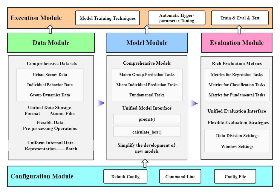
Figure 1: Overview of the LibCity library

Deep learning algorithms have been extensively used in urban spatial-temporal prediction in recent years, resulting in a wealth of research findings. However, according to our survey, less than 30% of the papers published in 11 leading conferences and journals have made their code and data open source, which hampers reproducibility in the field. Additionally, the need for recognized state-of-the-art (SOTA) models, standardized datasets, and transparent experimental settings creates obstacles to assessing the performance of new models and ultimately stifles innovation. In contrast, domains like Computer Vision, Natural Language Processing, and Recommendation Systems have standardized datasets such as IMAGENET [8] and algorithm libraries like MMDetection [9], and RecBole [10]. Unfortunately, urban spatial-temporal prediction lacks these resources. We propose LibCity, a comprehensive and unified library for urban spatial-temporal prediction, to address this issue.

Figure 1 illustrates the framework of LibCity, which comprises five main modules, including the data, model, evaluation, execution, and configuration module. Combining these modules forms a cohesive pipeline that provides researchers with a reliable experimental environment, and each module is responsible for a specific step in the pipeline. The subsequent sections will provide a detailed description of the implementation of each module.

• Data Module: Responsible for loading datasets and data preprocessing.

• Model Module: Responsible for initializing the reproduced baseline model or custom model.

• Evaluation Module: Responsible for evaluating model prediction results through multiple metrics.

• Execution Module: Responsible for model training and prediction.

• Configuration Module: Responsible for managing all the parameters involved in the framework.

5.1 Data Module

Our data module aims to address the issue of unfair evaluation caused by different data preparation methods by establishing a standardized data processing flow, as shown in Figure 2. This flow encompasses two types of data: user-oriented and model-oriented. The former establishes a unified storage format for spatial-temporal data, referred to as atomic files, which provides users with a consistent data input format. The latter defines a key-value data structure, known as Batch, to facilitate uniform data interaction between the data module and model module. Once the atomic files have been loaded and preprocessed, the Dataloader class in PyTorch is employed to convert the data into a Batch structure and then fed to the model module.

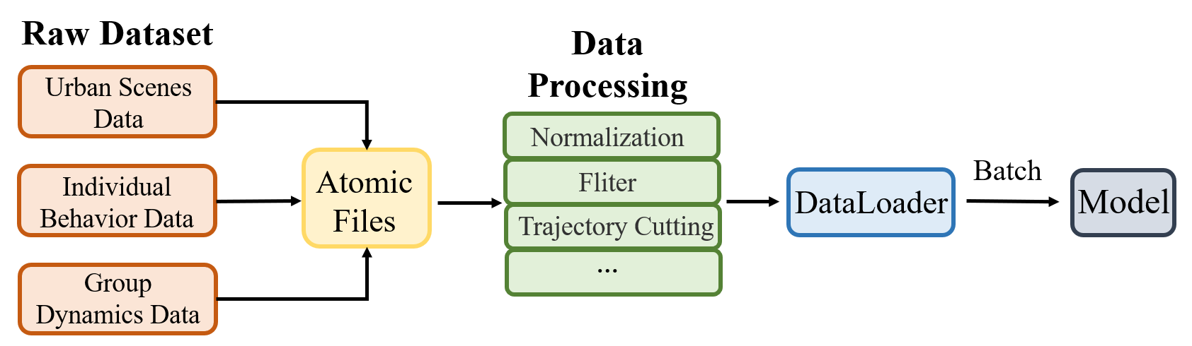
Figure 2: The data processing flow in LibCity

5.1.1 Atomic Files

LibCity defines a general and extensible data storage format for urban spatial-temporal data, i.e., atomic files. Atomic files contain five categories, the minor information units in spatial-temporal data. For more details, please refer to Section 3.2 above.

5.1.2 Preprocessing Operations

The LibCity library provides support for various data preprocessing operations. For the macro group prediction task, it is essential to normalize the spatial-temporal data to improve the model’s convergence toward the optimal solution. LibCity supports multiple data normalization methods, including Z-score normalization, min-max normalization, logarithmic normalization, and other custom normalization methods, which can be easily achieved through parameter settings. LibCity also supports the handling of missing values and outliers. For the micro individual prediction task, LibCity incorporates two trajectory filtering methods: inactive user filtering and inactive POI filtering. Inactive users can be filtered out by evaluating their activity based on the number and length of their trajectories and setting the minimum number of trajectories and minimum trajectory length. Similarly, inactive POIs can be filtered out based on the minimum number of visits. In this way, we can filter the data to reduce the impact of sparsity in spatial-temporal data.

5.1.3 Batch

The Batch is a key-value data structure based on the implementation of python.dict. It consists of feature names as keys and corresponding feature tensors (torch.Tensor) in a mini-batch as values. The purpose of the Batch is to facilitate data interaction between the data module and the model module in a systematic pipeline. In the pipeline, the executor extracts one Batch object from the Dataloader at a time and feeds it into the model. This structure enables the convenient use of feature tensors by referring to corresponding feature names. As different prediction models use varying features, they can all be stored in the form of Batch. Through this data form, LibCity can construct unified model interfaces and implement general executor for model training and testing, which is particularly useful for developing new models.

5.1.4 Comprehensive Datasets

We have conducted a comprehensive literature survey on spatial-temporal prediction and selected 351 representative papers, including survey papers. We identified all the open datasets used from these papers and selected 55 datasets based on their popularity, time span length, and data size. These datasets cover all the 9 tasks that LibCity supports, consisting of 40 group dynamics datasets (SSTD data), ten individual behavior datasets (SDTD data), and five urban scenes datasets (road network data). Table II, Table III, and Table IV provide statistics on these datasets. To facilitate the use of these datasets in LibCity, we have converted all of them into the atomic file format and created conversion tools, which can be found at this link.

TABLE II: Summary of Group Dynamics Datasets (SSTD Data) in LibCity

DATASET	#GEO	#REL	#DYNA	PLACE	DURATION	#TS	DATA TYPE
METR-LA [15]	207	11,753	7,094,304	Los Angeles, USA	Mar. 1, 2012 - Jun. 27, 2012	5min	Graph Speed
Los-Loop [33]	207	42,849	7,094,304	Los Angeles, USA	Mar. 1, 2012 - Jun. 27, 2012	5min	Graph Speed
SZ-Taxi [33]	156	24,336	464,256	Shenzhen, China	Jan. 1, 2015 - Jan. 31, 2015	15min	Graph Speed
Q-Traffic [34]	45,148	63,422	264,386,688	Beijing, China	Apr. 1, 2017 - May 31, 2017	15min	Graph Speed
Loop Seattle [35, 36]	323	104,329	33,953,760	Greater Seattle Area, USA	Jan. 1, 2015 - Dec. 31, 2015	5min	Graph Speed
PEMSD7(M) [16]	228	51,984	2,889,216	California, USA	Weekdays of May. Jun., 2012	5min	Graph Speed
PEMS-BAY [15]	325	8,358	16,937,700	San Francisco Bay Area, USA	Jan. 1, 2017 - Jun. 30, 2017	5min	Graph Speed
Rotterdam [37]	208	-	4,813,536	Rotterdam, Holland	135 days of 2018	2min	Graph Speed
PeMSD3 [38]	358	547	9,382,464	California, USA	Sept. 1, 2018 - Nov. 30, 2018	5min	Graph Flow
PEMSD7 [38]	883	866	24,921,792	California, USA	Jul. 1, 2016 - Aug. 31, 2016	5min	Graph Flow
Beijing subway [39]	276	76,176	248,400	Beijing, China	Feb. 29, 2016 - Apr. 3, 2016	30min	Graph Flow
M-dense [40]	30	-	525,600	Madrid, Spain	Jan. 1, 2018 - Dec. 21, 2019	60min	Graph Flow
SHMetro [41]	288	82,944	1,934,208	Shanghai, China	Jul. 1, 2016 - Sept. 30, 2016	15min	Graph Flow
HZMetro [41]	80	6,400	146,000	Hangzhou, China	Jan. 1, 2019 - Jan. 25, 2019	15min	Graph Flow
NYCTaxi-Dyna	263	69,169	574,392	New York, USA	Jan. 1, 2020 - Mar. 31, 2020	60min	Region Flow
PeMSD4 [42]	307	340	5,216,544	San Francisco Bay Area, USA	Jan. 1, 2018 - Feb. 28, 2018	5min	Graph Flow, Speed, Occupancy
PEMSD8 [42]	170	277	3,035,520	San Bernardino Area, USA	Jul. 1, 2016 - Aug. 31, 2016	5min	Graph Flow, Speed, Occupancy
TaxiBJ2013 [14]	32*32	-	4,964,352	Beijing, China	Jul. 1, 2013 - Oct. 30, 2013	30min	Grid In&Out Flow
TaxiBJ2014 [14]	32*32	-	4,472,832	Beijing, China	Mar. 1, 2014 - Jun. 30, 2014	30min	Grid In&Out Flow
TaxiBJ2015 [14]	32*32	-	5,652,480	Beijing, China	Mar. 1, 2015 - Jun. 30, 2015	30min	Grid In&Out Flow
TaxiBJ2016 [14]	32*32	-	6,782,976	Beijing, China	Nov. 1, 2015 - Apr. 10, 2016	30min	Grid In&Out Flow
T-Drive [43, 44]	32*32	-	3,686,400	Beijing, China	Feb. 1, 2015 - Jun. 30, 2015	60min	Grid In&Out Flow
Porto	20*10	-	441,600	Porto, Portugal	Jul. 1, 2013 - Sept. 30, 2013	60min	Grid In&Out Flow
NYCTaxi140103	10*20	-	432,000	New York, USA	Jan. 1, 2014 - Mar. 31, 2014	60min	Grid In&Out Flow
NYCTaxi140112 [45]	15*5	-	1,314,000	New York, USA	Jan. 1, 2014 - Dec. 31, 2014	30min	Grid In&Out Flow
NYCTaxi150103 [46]	10*20	-	576,000	New York, USA	Jan. 1, 2015 - Mar. 1, 2015	30min	Grid In&Out Flow
NYCTaxi160102 [47]	16*12	-	552,960	New York, USA	Jan. 1, 2016 - Feb. 29, 2016	30min	Grid In&Out Flow
NYCBike140409 [14]	16*8	-	562,176	New York, USA	Apr. 1, 2014 - Sept. 30, 2014	60min	Grid In&Out Flow
NYCBike160708 [46]	10*20	-	576,000	New York, USA	Jul. 1, 2016 - Aug. 29, 2016	30min	Grid In&Out Flow
NYCBike160809 [47]	14*8	-	322,560	New York, USA	Aug. 1, 2016 - Sept. 29, 2016	30min	Grid In&Out Flow
NYCBike200709	10*20	-	441,600	New York, USA	Jul. 1, 2020 - Sept. 30, 2020	60min	Grid In&Out Flow
AustinRide	16*8	-	282,624	Austin, USA	Jul. 1, 2016 - Sept. 30, 2016	60min	Grid In&Out Flow
BikeDC	16*8	-	282,624	Washington, USA	Jul. 1, 2020 - Sept. 30, 2020	60min	Grid In&Out Flow
BikeCHI	15*18	-	596,160	Chicago, USA	Jul. 1, 2020 - Sept. 30, 2020	60min	Grid In&Out Flow
NYCTaxi-OD	263	69,169	150,995,927	New York, USA	Apr. 1, 2020 - Jun. 30, 2020	60min	OD Flow
NYC-TOD [48]	15*5	-	98,550,000	New York, USA	Jan. 1, 2014 - Dec. 31, 2014	30min	Grid-OD Flow
NYCTaxi150103 [46]	10*20	-	115,200,000	New York, USA	Jan. 1, 2015 - Mar. 1, 2015	30min	Grid-OD Flow
NYCBike160708 [46]	10*20	-	115,200,000	New York, USA	Jul. 1, 2016 - Aug. 29, 2016	30min	Grid-OD Flow
NYC-Risk [49]	243	59,049	3,504,000	New York, USA	Jan. 1, 2013 - Dec. 31, 2013	60min	Risk
CHI-Risk [49]	243	59,049	3,504,000	New York, USA	Jan. 1, 2013 - Dec. 31, 2013	60min	Risk

TABLE III: Summary of Individual Behavior Datasets (SDTD Data) in LibCity

DATASET	#GEO	#REL	#USR	#DYNA	PLACE	DURATION	DATA TYPE
Seattle [50]	613,645	857,406	1	7,531	Seattle WA, USA	Jan. 17, 2009	GPS-based
Global [51]	11,045	18,196	1	2,502	100 cities	-	GPS-based
CD-Taxi-Sample [52]	-	-	4,565	712,360	Chengdu, China	Aug. 3, 2014 - Aug. 30, 2014	GPS-based
BJ-Taxi-Sample [52]	16,384	-	76	518,424	Beijing, China	Oct. 1, 2013 - Oct. 31, 2013	GPS-based
Porto [53]	10,903	26,161	435	695,085	Porto, Portugal	Jul. 1, 2013 - Jul. 1, 2014	Road-network Constrained
Foursquare-TKY [54]	61,857	-	2,292	573,703	Tokyo, Japan	Apr. 4, 2012 - Feb. 16, 2013	POI-based
Foursquare-NYC [54]	38,332	-	1,082	227,428	New York, USA	Apr. 3, 2012 - Feb. 15, 2013	POI-based
Gowalla [55]	1,280,969	913,660	107,092	6,442,892	Global	Feb. 4, 2009 - Oct. 23, 2010	POI-based
BrightKite [55]	772,966	394,334	51,406	4,747,287	Global	Mar. 21, 2008 - Oct. 18, 2010	POI-based
Instagram [56]	13,187	-	78,233	2,205,794	New York, USA	Jun. 15, 2011 - Nov. 8, 2016	POI-based

TABLE IV: Summary of Urban Scenes Datasets (Road Network Data) in LibCity

DATASET	#GEO	#REL	PLACE
BJ-Roadmap-Edge [53]	40,306	101,024	Beijing, China
BJ-Roadmap-Node	16,927	38,027	Beijing, China
CD-Roadmap-Edge	6,195	15,962	Chengdu, China
XA-Roadmap-Edge	5,269	13,032	Xian, China
Porto-Roadmap-Edge [53]	11,095	26,161	Porto, Portugal

5.2 Model Module

To increase the modularity of the library and reduce coupling between different modules, LibCity uses a separate model module to implement classic spatial-temporal prediction algorithms. This module contains various models such as LSTM, GRU, TCN, GCN, etc. Encapsulating each model in a separate class, LibCity enables users to easily switch between different models and extend the library with new ones.

5.2.1 Unified Interface

In specific, LibCity provides two standard interfaces for all urban spatial-temporal prediction models: predict() and calculate_loss() functions as follows:

• The predict() function is used in the process of model prediction to return the model prediction results.

• The calculate_loss() function is used in the model training process to return the loss value, which needs to be optimized.

Both methods take the internal data representation Batch as input. These interface functions are general to different spatial-temporal prediction models, which allows researchers to implement various models in a highly unified way. When developing a new model, researchers only need to instantiate these two interfaces to connect with other modules in LibCity. They do not need to worry about how each of the other parts works. This design simplifies the development process and accelerates the development of new models.

5.2.2 Implemented Models

Currently, LibCity supports 9 mainstream spatial-temporal prediction tasks. Through careful investigation of the development process in the field of spatial-temporal prediction, we have selected 65 classic spatial-temporal prediction models to reproduce, ranging from early CNN-based models to recent GCN-based models and hybrid models. Moreover, in order to cover a wide range of prediction models, we also implement four shallow baseline models. We have tested all implemented models’ performance on at least two datasets. We summarize the implemented 65 models in Table V. Referring to Section LABEL:macro_models, we also provide in the table the different basic structures of the model in the spatial and temporal dimensions. Users can refer to this table to learn about the main techniques and developments in the field of urban spatial-temporal prediction.

TABLE V: Implement Models in LibCity

Task	Model	Conference	Year	Spatial Axis			Temporal axis
				CNN	GCN	Attn.	LSTM	GRU	TCN	Attn.
Traditional Methods	HA	-	-	-	-	-	-	-	-	-
	SVR [57]	NIPS	1996	-	-	-	-	-	-	-
	ARIMA [58]	J TRANSP ENG	2003	-	-	-	-	-	-	-
	VAR [59]	Princeton Press	1994	-	-	-	-	-	-	-
General Macro Group Prediction	RNN [60]	NIPS	2014				✓	✓
	Seq2Seq [60]	NIPS	2014				✓	✓
	AutoEncoder [61]	IEEE TITS	2014	-	-	-	-	-	-	-
	FNN [15]	ICLR	2018	-	-	-	-	-	-	-
Traffic Flow Prediction	ST-ResNet [14]	AAAI	2017	✓
	STNN [62]	ICDM	2017	-	-	-	-	-	-	-
	ACFM [45]	ACM MM	2018	✓		✓	✓
	STDN [46]	AAAI	2019	✓			✓			✓
	ASTGCN [42]	AAAI	2019		✓	✓			✓	✓
	MSTGCN [42]	AAAI	2019		✓				✓
	DSAN [47]	KDD	2020			✓				✓
	STSGCN [38]	AAAI	2020		✓
	AGCRN [63]	NIPS	2020		✓			✓
	CRANN [64]	arXiv	2020	✓		✓	✓
	CONVGCN [65]	IET ITS	2020	✓	✓
	ResLSTM [39]	IEEE TITS	2020		✓		✓			✓
	MultiSTGCnet [66]	IJCNN	2020		✓		✓
	ToGCN [67]	IEEE TITS	2021		✓		✓
	DGCN [68]	IEEE TITS	2022		✓	✓	✓		✓	✓
Traffic Speed Prediction	DCRNN [15]	ICLR	2018		✓			✓
	STGCN [16]	IJCAI	2018		✓				✓
	GWNET [69]	IJCAI	2019		✓				✓
	TGCN [33]	IEEE TITS	2019		✓			✓
	TGCLSTM [36]	IEEE TITS	2019		✓		✓
	MTGNN [70]	KDD	2020		✓				✓
	GMAN [71]	AAAI	2020			✓				✓
	ATDM [72]	NCA	2021		✓		✓
	STAGGCN [73]	CIKM	2020		✓	✓			✓	✓
	ST-MGAT [74]	ICTAI	2020			✓			✓
	DKFN [75]	ACM GIS	2020		✓		✓
	STTN [76]	arXiv	2020		✓	✓				✓
	HGCN [77]	AAAI	2021		✓				✓	✓
	GTS [78]	ICLR	2021		✓			✓
On-Demand Service Prediction	DMVSTNet [17]	AAAA	2018	✓			✓
	STG2Seq [79]	IJCAI	2019		✓					✓
	CCRNN [80]	AAAI	2021		✓			✓
Traffic Accident Prediction	GSNet [49]	AAAI	2021		✓			✓		✓
OD Matrix Prediction	GEML [81]	KDD	2019		✓		✓
	CSTN [48]	IEEE TITS	2019	✓			✓
Trajectory Next-Location Prediction	FPMC [82]	WWW	2010
	LSTM [83]	CoRR	2013				✓
	ST-RNN [25]	AAAI	2016					✓
	SERM [84]	CIKM	2017					✓
	DeepMove [26]	WWW	2017				✓			✓
	CARA [85]	SIGIR	2018					✓
	HSTLSTM [86]	IJCAI	2018				✓
	ATSTLSTM [87]	IEEE TSC	2019				✓			✓
	LSTPM [88]	AAAI	2020					✓		✓
	GeoSAN [89]	KDD	2020							✓
	STAN [90]	WWW	2021							✓
Travel Time Prediction	DeepTTE [52]	AAAI	2018	✓			✓
	TTPNet [91]	TKDE	2022	✓			✓
Map Matching	STMatching [92]	ACM GIS	2009	-	-	-	-	-	-	-
	HMMM [50]	ACM GIS	2009	-	-	-	-	-	-	-
	IVMM [93]	IEEE MDM	2010	-	-	-	-	-	-	-
Road Network Representation Learning	DeepWalk [94]	KDD	2014	-	-	-	-	-	-	-
	LINE [95]	WWW	2015	-	-	-	-	-	-	-
	Node2Vec [96]	KDD	2016	-	-	-	-	-	-	-
	ChebConv [97]	NIPS	2016		✓
	GAT [98]	arXiv	2017			✓
	GeomGCN [99]	ICLR	2020		✓

5.3 Evaluation Module

With the standardized data processing flow and prediction model interfaces, LibCity also offers standard evaluation procedures for spatial-temporal prediction tasks. Since the model output formats and evaluation metrics may vary across different spatial-temporal prediction tasks, LibCity develops specific evaluators for each task and supports various popular evaluation metrics.

5.3.1 Evaluation Metrics

Metrics for Regression Tasks: In LibCity, regression tasks consist of Traffic Flow Prediction, Traffic Speed Prediction, On-Demand Service Prediction, Origin-Destination Matrix Prediction, Traffic Accidents Prediction, and Travel Time Prediction. These tasks output real numbers and are evaluated using commonly used value-based metrics, which include Mean Absolute Error (MAE), Mean Squared Error (MSE), Root Mean Squared Error (RMSE), Mean Absolute Percentage Error (MAPE), Coefficient of Determination ($R^{2}$), and Explained Variance Score (EVAR). Their calculation formulas for these metrics are as follows:

$$\small MAE=\frac{1}{n}\sum_{i=1}^{n}|\hat{y_{i}}-y_{i}|$$ (3)

$$\small MSE=\frac{1}{n}\sum_{i=1}^{n}(\hat{y_{i}}-y_{i})^{2}$$ (4)

$$\small RMSE=\sqrt{\frac{1}{n}\sum_{i=1}^{n}(\hat{y_{i}}-y_{i})^{2}}$$ (5)

$$\small MAPE=\frac{1}{n}\sum_{i=1}^{n}|\frac{\hat{y_{i}}-y_{i}}{y_{i}}|*100\%$$ (6)

$$\small R^{2}=1-\frac{\sum_{i=1}^{n}(y_{i}-\hat{y_{i}})^{2}}{\sum_{i=1}^{n}(y_{i}-\bar{y})^{2}}$$ (7)

$$\small EVAR=1-\frac{Var(y_{i}-\hat{y_{i}})}{Var(y_{i})}$$ (8)

where $\bm{y}=\{y_{1},y_{2},...,y_{n}\}$ is the ground-truth value, $\hat{\bm{y}}=\{\hat{y_{1}},\hat{y_{2}},...,\hat{y_{n}}\}$ is the prediction value, $n$ is the number of samples, $\bar{y}=\frac{1}{n}\sum_{i=1}^{n}y_{i}$ is the mean value, $Var(y_{i})=\frac{1}{n}\sum_{i=1}^{n}(y_{i}-\bar{y})^{2}$ is the variance.

Metrics for Classification Tasks: The classification task in LibCity is Trajectory Next-Location Prediction. The output of this task in LibCity is a probability distribution over the candidate’s next locations. The Trajectory Next-Location Prediction task is evaluated using various rank-based metrics, including Precision@K, Recall@K, F1-score@K, MRR@K (Mean Reciprocal Rank@K), and NDCG@K (Normalized Discounted Cumulative Gain@K). The calculation formulas for these metrics are as follows:

$$\small Precision@K=\frac{\sum_{i=1}^{N}|\operatorname{Hit}(i)|}{N\times K}$$ (9)

$$\small Recall@K=\frac{\sum_{i=1}^{N}|\operatorname{Hit}(i)|}{N}$$ (10)

$$\small F1@K=\frac{2\times\text{ Precision@ }\times\text{ Recall@ }K}{\text{ Precision }@+\text{ Recall@ }K}$$ (11)

$$\small MRR@K=\frac{1}{N}\sum_{i=1}^{N}\frac{1}{\operatorname{Rank}(i)}$$ (12)

$$\small NDCG@K=\frac{1}{N}\sum_{i=1}^{N}\frac{1}{\log_{2}(\operatorname{rank}(i)+1)}$$ (13)

where $N$ is the number of test data, $i$ is the $i$-th test data, $K$ is the top $K$ prediction outputs for evaluation, $T(i)$ is the real next hop position in the $i$-th test data, $R(i)$ is the set of the top K locations in the prediction result of the $i$-th test data, $Hit(i)$ is the set of predicted hit locations in the $i$-th test data, which means $T(i)\cap R(i)$, $Rank(i)$ is the ranking of $T(i)$ in $R(i)$ in the $i$-th test data, and $|*|$ is the modulo operator of a set.

Metrics for Fundamental Tasks: Fundamental tasks in LibCity provide support for macro and micro prediction tasks, including map matching and road network representation learning. The road network representation task requires combining with specific downstream tasks to evaluate the performance of the representation vectors. For instance, if a road segment classification task is used for evaluation, it is a classification task. If a road flow prediction task is used for evaluation, it is a regression task. The evaluation metrics for these tasks are similar to the ones described above. Here we focus on the evaluation metrics for the map matching task.

LibCity evaluates the map matching task using three metrics: RMF (Route Mismatch Fraction), AN (Accuracy in Number), and AL (Accuracy in Length), which have been used in previous works such as [50, 93].

$$\small RMF=\frac{d_{-}+d_{+}}{d_{0}}$$ (14)

$$\small AN=\frac{\#Rc}{\#R}$$ (15)

$$\small AL=\frac{\sum len(Rc)}{\sum len(R)}$$ (16)

where $d_{0}$ denotes the length subtracted from the error, $d_{+}$ denotes the length added to the error, $d_{-}$ is the total length of the real path, $Rc$ denotes correctly matched roads, $R$ denotes all roads of the real route. $len()$ denotes the length of a set of roads.

5.3.2 Evaluation Strategies

To evaluate the performance of spatial-temporal prediction models in a flexible manner, LibCity offers two main strategies.

Firstly, users can divide the dataset into training, validation, and testing sets with a ratio of their choice. The training set is used for model training, while the validation set is used for hyper-parameter tuning and preventing overfitting. The testing set is used to evaluate the final performance of the trained model.

Secondly, LibCity allows users to set different window sizes for evaluation. For macro group prediction tasks, users can set various input and output time windows, and LibCity will partition the input data based on the window size, enabling multi-step predictions using historical observations of different lengths. For micro individual prediction tasks, trajectories are split based on window settings, with options for time-based or length-based windows. Users can set the window size and type to evaluate the model’s performance on trajectories of varying lengths, such as long, medium, and short trajectories.

These two strategies can be combined with various evaluation metrics to perform comprehensive evaluations of models for the same task, providing greater flexibility and adaptability in assessing model performance.

5.4 Execution Module

The execution module in LibCity serves as the central hub that controls the interactions between other modules to facilitate model training and performance evaluation. Users can modify the parameter settings of this module to adjust the effect of model training. It supports various model training strategies that optimize the model and includes a built-in automatic hyper-parameter tuning module to reduce the user’s workload and achieve automatic optimization of the model.

5.4.1 Model Training Techniques

LibCity offers various training techniques to train deep neural networks effectively. These techniques can be customized by modifying the parameter settings of the execution module. Here are some of the techniques supported by LibCity:

• Optimizer options: During the training of a deep learning model, the optimizer is mainly used to update the parameters of the network in order to minimize the loss function. LibCity supports several optimizers including SGD [100], RMSProp [101], Adam [102], and AdaGrad [103]. Different optimization algorithms have different ways of updating the network parameters and are better suited to different scenarios. Users can choose the appropriate optimization algorithm for their usage scenarios to achieve better training results.

• Learning rate adjustment strategies: Learning rate is a key parameter of neural network models, which controls the speed of gradient-based adjustment of network weights and determines the convergence of the loss function to the optimal solution.

• Loss Function options: Various loss functions are used in deep learning and different loss functions compute the loss in different ways to obtain different training results. LibCity supports five types of loss functions including Cross-entropy Loss, L1 Loss, L2 Loss, Huber Loss [104], LogCosh Loss [105], and Quantile Loss [106].

• Early Stopping: Overfitting may occur as the number of training rounds increases. LibCity supports the early stopping method to prevent overfitting. Users can specify whether to use the early stop mechanism and the size of the duration rounds through parameter configuration.

• Gradient Clipping: Gradient explosion may occur during training. To avoid this, LibCity supports gradient clipping strategies [107]. Users can specify whether to use gradient clipping through parameter configuration.

5.4.2 Automatic Hyper-parameter Tuning

Hyper-parameter tuning has a significant impact on the performance of deep learning models. To ease the burden of manual parameter tuning, LibCity provides an automatic hyper-parameter tuning mechanism. We implement this feature using the third-party library Ray Tune[108], which supports various search algorithms such as Grid Search, Random Search, and Bayesian Optimization. Users can specify the parameters to be tuned and their search space in a configuration file and select the tuning method. LibCity will then sample multiple times from the search space and run the model in a distributed manner, automatically saving the best parameter values and corresponding model prediction results. An example of automatic hyper-parameter tuning is presented in Section 6.2.

5.5 Configuration Module

LibCity utilizes the configuration module to set the parameters for the entire framework. The experiment parameter configuration is determined by three factors: parameters passed from the command line, user-defined configuration file, and default configuration files of the modules in LibCity. The priority of the above three parameter configuration methods decreases in order, with higher priority parameters overriding lower priority parameters with the same name. With this priority design, users can flexibly adjust the parameter configuration of an experiment through the first two methods.

To adjust parameters through the command line, users only need to use ”–parameter_name” when running LibCity. However, it is important to note that only frequently adjusted parameters in an experiment, such as batch size and learning rate, are allowed to be passed from the command line. In order to allow users to modify default parameters more extensively, LibCity allows users to pass the name of a user-defined configuration file through the command line, which is then read by the system to set the parameter configuration.

5.6 Experiment Management and Visualization Platform

(a) Platform Homepage

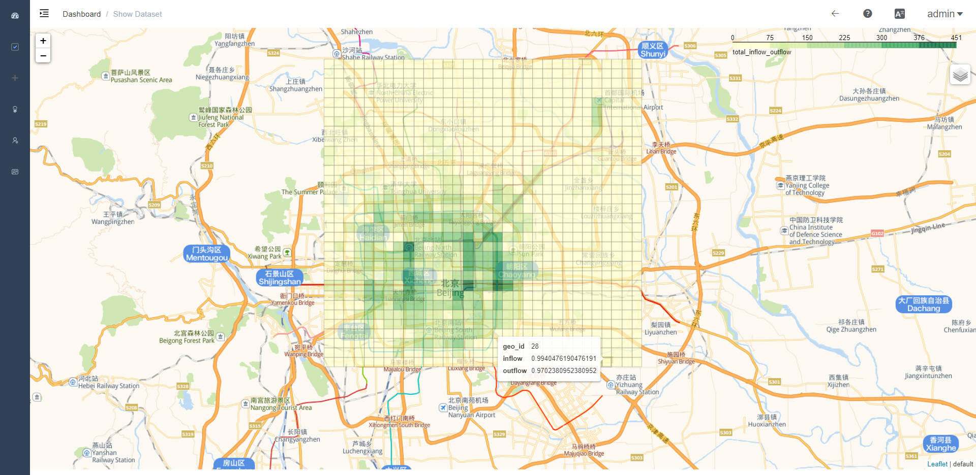
(b) Visualization of Beijing Flow Dataset

(c) Create Experiment

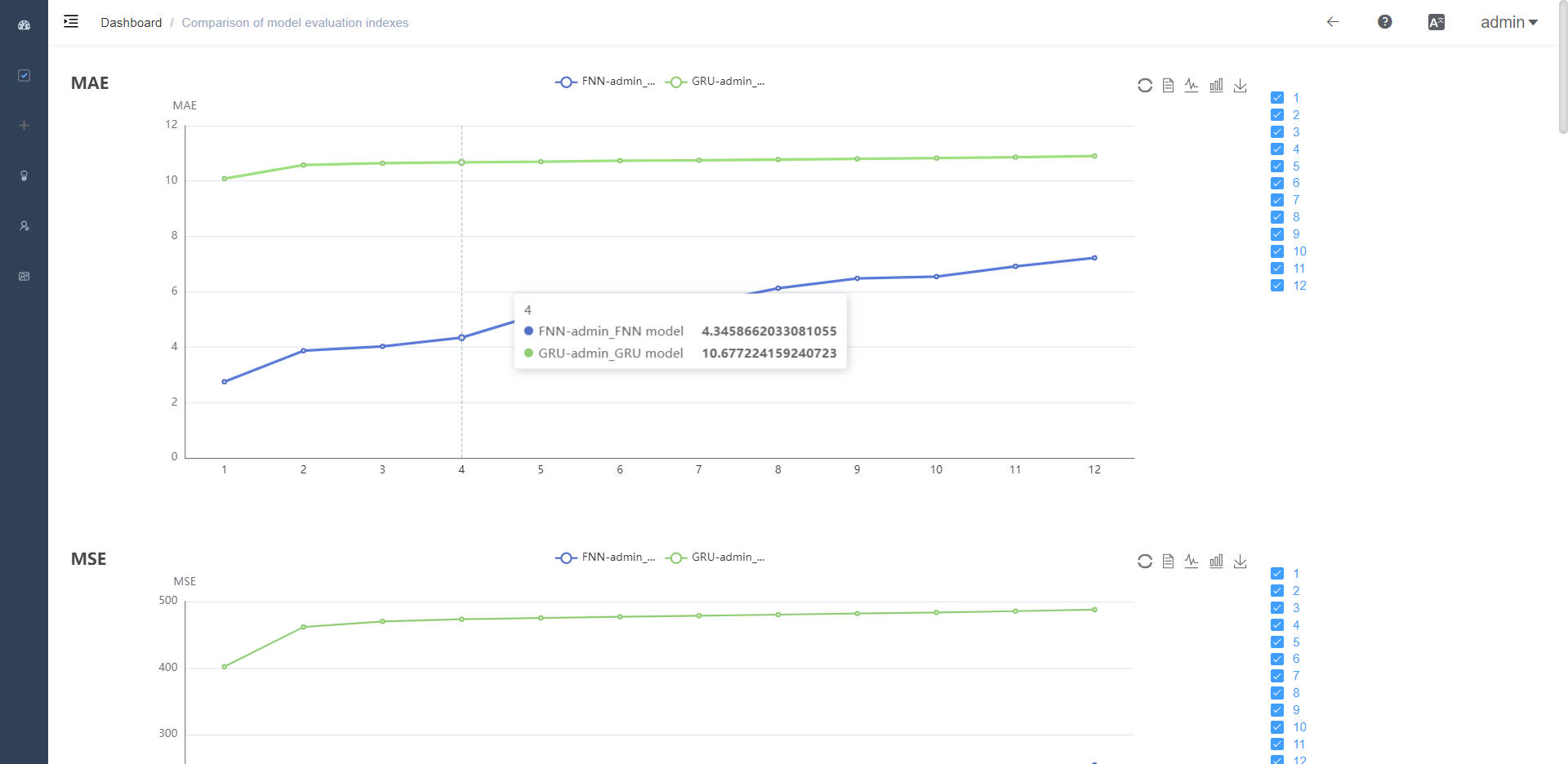
(d) Model Performance Comparison

Figure 3: Experiment Management and Visualization Platform

We have created a web-based experiment management and visualization platform for convenient experimentation with LibCity’s models and datasets as shown in Figure 3(a). The platform features a user-friendly graphical interface and comprehensive functionalities to support spatial-temporal prediction research. Users can easily upload new datasets and visualize them, as demonstrated in Figure 3(b), which shows the visualization of the Beijing traffic flow dataset. After configuring the model’s parameters, users can create new experiments through a straightforward web interface, as shown in Figure 3(c). They can then execute the experiments at their convenience, with the training logs available for viewing during the experiment. After the experiment’s execution, users can obtain evaluation results of the model on specific metrics and visualize the prediction results. Additionally, the platform offers an experimental comparison function, allowing users to compare the performance of different models shown in Figure 3(d).

We have built the experiment management and visualization platform using Django, Vue, and MySQL. The platform’s open-sourced code can be found on GitHub.

6 Usage Examples of LibCity

This section provides several examples of using LibCity to assist users in getting started with the framework. The examples cover running existing models, conducting automatic parameter tuning, and adding new models to LibCity.

6.1 Running Existing Models

The general process of running existing models in LibCity is listed as follows:

1. Dataset formatting: Users must download and convert the raw dataset into atomic files.

2. Configuration setup: Users can configure the experiment parameters through a configuration file, the command line, or the default parameters of LibCity. The configuration module’s parameters form the foundation of the entire framework.

3. Dataset pre-processing and splitting: Based on the user’s parameter settings, LibCity pre-processes and splits the dataset. Users can specify custom dataset division ratios and data pre-processing thresholds. For example, users may filter out trajectories with lengths less than 5.

4. Model initialization: LibCity creates a model object based on the user’s task and model name selection.

5. Training and evaluation: Once the data and model are ready, LibCity calls the executor module to train and evaluate the model on the specified dataset. The training logs, trained models, and model evaluation results are automatically saved for the user’s use.

The above steps are performed automatically by LibCity’s unified entry file (run_model.py). Users need only execute a single command in the command line to initiate the model running process. Three essential parameters must be specified at runtime, namely the task, model, and dataset, via –task, –model, and –dataset options, respectively. For example, running the GRU model on the METR_LA dataset for 50 epochs on the second GPU block requires the following command:

python run_model.py –task traffic_state_prediction –model GRU –dataset METR_LA –gpu 2 –epoch 50

6.2 Running Automatic Parameter Tuning

Considering that hyper-parameter tuning significantly impacts the performance of deep learning models, LibCity has introduced an automatic hyper-parameter tuning mechanism that can easily optimize a given model based on the user-provided hyper-parameter range. The general steps for running the automatic tuning function are as follows:

1. Setting the hyper-parameter search space. Users must specify the hyper-parameters to be tuned and their corresponding value ranges in a JSON file. For example, the search space for the hidden layer dimension parameter can be a discrete set of categorical variables, such as [50, 100, 200]. The user can specify the file name of the parameter space file using the parameter –space_file.

2. Selecting the tuning method. LibCity uses the third-party library Ray Tune [108] to implement automatic hyper-parameter tuning, which supports various search algorithms, including Grid Search, Random Search, and Bayesian Optimization. The user can select the tuning method by specifying the parameter –search_alg.

3. Starting the tuning process. Users can execute a single command in the command line to automatically tune the model parameters. During the tuning process, LibCity will sample the corresponding parameter values from the search space and perform model training and validation. After all the samples are validated, the script will output the best parameter combination on the terminal and save them to a log file. Here is an example of the command to run the automatic tuning function: python hyper_tune.py –task traffic_state_pred –model GRU –dataset METR_LA –search_alg BasicSearch –space_file sample_space_file

6.3 Implementing a New Model

The modular design and unified interface definition of LibCity provide flexibility for user-defined extensions and excellent scalability. Developing a new spatial-temporal prediction model using LibCity is straightforward. The general process for developing a new model using LibCity is as follows:

1. Create a new model file and define a model class that inherits from the existing model abstraction class provided by LibCity. All 9 tasks supported by LibCity have their abstract classes implemented.

2. Implement the __init__() function to initialize the model according to the configuration parameters. The input parameter config contains the configuration information.

3. Implement the calculate_loss() function to calculate the loss between the predicted result and the true value during model training. The goal of model training is to optimize this loss.

4. Implement the predict() function to return the model prediction results during prediction.

5. Configure the default parameter configuration file for the new model to specify the required parameters and their values for running the model.

6. Run the model and evaluate its performance on the selected dataset.

Thus, developing new models using LibCity is simplified by focusing on implementing only three interfaces, while LibCity handles other details like data splitting, model training, and performance evaluation. This design approach simplifies the development process of new models and highlights the scalability of LibCity.

7 Comparison with Existing Libraries

TABLE VI: Comparison with existing libraries by 2023/4/22

Framework\Metric	Modularization	#Fork	#Star	#Models	#Datasets	#Issues
DL-Traff	Low	34	179	18	7	2/3
DGCRN	Low	64	173	12	3	9/13
FOST	Middle	43	208	6	0	4/13
LibCity	High	111	485	65	55	0/73

To the best of our knowledge, LibCity [6] is the first spatial-temporal prediction library that enables researchers to conduct comprehensive comparative experiments and develop new models. Recently, other researchers have proposed benchmarks in spatial-temporal prediction similar to LibCity. This section compares with others to demonstrate the advantages of LibCity.

DL-Traff [109] is an open-source project offering a traffic prediction benchmark using grid-based and graph-based models. DGCRN [110] summarizes previous work and produces a benchmark in traffic prediction. However, these two projects only accumulate the model codes from past research work without a modular design, which makes it inconvenient for users to use. Furthermore, they only focus on macro-level traffic prediction without contributing to micro-level individual prediction tasks. Microsoft FOST  (Forecasting Open Source Tool) is a general forecasting tool that aims to provide an easy-to-use tool for spatial-temporal forecasting, but its supported models and applications are limited.

Table VI illustrates that LibCity outperforms the other compared tools in terms of the number of models and datasets it can handle. Furthermore, LibCity designs a unified storage format for spatial-temporal data, which is a great help to promote the standardization of the field. The modular design of LibCity allows for scalability and enables developers to easily create new models using its pipeline. The high number of Stars and Forks indicates that LibCity is popular among the open-source community. The number of open issues and total issues also suggests that the developers of LibCity are active in the community, which helps to address user inquiries and promote further development in the field.

In addition, it is worth noting that numerous similar experimental libraries are available in other research fields. For instance, RecBole [10] is a recommendation algorithm framework that reproduces a vast range of recommendation models and provides various evaluation strategies and data preprocessing operations, making it easy to conduct experiments. Meanwhile, MMDetection [9] adopts a modular design, enabling researchers to efficiently develop new models based on it for object detection tasks. FastReID [111] continuously reproduces state-of-the-art models and releases corresponding pre-trained models for both research and industrial purposes.

LibCity combines the strengths of the libraries as mentioned above, such as various baseline models, diverse evaluation strategies, and modular design. As a result, it not only facilitates researchers to conduct experiments and develop new models but also promotes standardization within the spatial-temporal prediction field.

8 Conclusion

In this work, we present a comprehensive review of urban spatial-temporal prediction and proposes a unified storage format for spatial-temporal data, called atomic files. Building on this, we introduce LibCity, a unified and comprehensive open-source library for urban spatial-temporal prediction that includes 55 spatial-temporal datasets and 65 spatial-temporal prediction models covering 9 mainstream sub-tasks of urban spatial-temporal prediction. By conducting extensive experiments using LibCity, we establish a comprehensive model performance leaderboard that identifies promising research directions for spatial-temporal prediction.

To the best of our knowledge, LibCity is the first open-source library for urban spatial-temporal prediction, providing a valuable tool for exploring and developing spatial-temporal prediction models. We will continuously expand LibCity to contribute to the spatial-temporal prediction field in the future. For example, we can cover more spatial-temporal prediction tasks, such as climate prediction, air quality prediction, theft prediction, etc.

References

- [1] X. Yin, G. Wu, J. Wei, Y. Shen, H. Qi, and B. Yin, “Deep learning on traffic prediction: Methods, analysis and future directions,” IEEE Transactions on Intelligent Transportation Systems, 2021.
- [2] K. Gu, J. Hu, and W. Jia, “Adaptive area-based traffic congestion control and management scheme based on fog computing,” IEEE Trans. Intell. Transp. Syst., vol. 24, no. 1, pp. 1359–1373, 2023.
- [3] B. Li, T. Dai, W. Chen, X. Song, Y. Zang, Z. Huang, Q. Lin, and K. Cai, “T-PORP: A trusted parallel route planning model on dynamic road networks,” IEEE Trans. Intell. Transp. Syst., vol. 24, no. 1, pp. 1238–1250, 2023.
- [4] M. Zhou, J. Jin, W. Zhang, Z. T. Qin, Y. Jiao, C. Wang, G. Wu, Y. Yu, and J. Ye, “Multi-agent reinforcement learning for order-dispatching via order-vehicle distribution matching,” in CIKM. ACM, 2019, pp. 2645–2653.
- [5] H. Zang, D. Han, X. Li, Z. Wan, and M. Wang, “CHA: categorical hierarchy-based attention for next POI recommendation,” ACM Trans. Inf. Syst., vol. 40, no. 1, pp. 7:1–7:22, 2022.
- [6] J. Wang, J. Jiang, W. Jiang, C. Li, and W. X. Zhao, “Libcity: An open library for traffic prediction,” in SIGSPATIAL/GIS. ACM, 2021, pp. 145–148.
- [7] D. A. Tedjopurnomo, Z. Bao, B. Zheng, F. M. Choudhury, and A. K. Qin, “A survey on modern deep neural network for traffic prediction: Trends, methods and challenges,” IEEE Trans. Knowl. Data Eng., vol. 34, no. 4, pp. 1544–1561, 2022.
- [8] J. Deng, W. Dong, R. Socher, L. Li, K. Li, and L. Fei-Fei, “Imagenet: A large-scale hierarchical image database,” in CVPR. IEEE Computer Society, 2009, pp. 248–255.
- [9] K. Chen, J. Wang, J. Pang, Y. Cao, Y. Xiong, X. Li, S. Sun, W. Feng, Z. Liu, J. Xu, Z. Zhang, D. Cheng, C. Zhu, T. Cheng, Q. Zhao, B. Li, X. Lu, R. Zhu, Y. Wu, J. Dai, J. Wang, J. Shi, W. Ouyang, C. C. Loy, and D. Lin, “Mmdetection: Open mmlab detection toolbox and benchmark,” CoRR, vol. abs/1906.07155, 2019.
- [10] W. X. Zhao, S. Mu, Y. Hou, Z. Lin, Y. Chen, X. Pan, K. Li, Y. Lu, H. Wang, C. Tian, Y. Min, Z. Feng, X. Fan, X. Chen, P. Wang, W. Ji, Y. Li, X. Wang, and J. Wen, “Recbole: Towards a unified, comprehensive and efficient framework for recommendation algorithms,” in CIKM. ACM, 2021, pp. 4653–4664.
- [11] A. Paszke, S. Gross, F. Massa, A. Lerer, J. Bradbury, G. Chanan, T. Killeen, Z. Lin, N. Gimelshein, L. Antiga, A. Desmaison, A. Köpf, E. Z. Yang, Z. DeVito, M. Raison, A. Tejani, S. Chilamkurthy, B. Steiner, L. Fang, J. Bai, and S. Chintala, “Pytorch: An imperative style, high-performance deep learning library,” in NeurIPS, 2019, pp. 8024–8035.
- [12] J. Ye, J. Zhao, K. Ye, and C. Xu, “How to build a graph-based deep learning architecture in traffic domain: A survey,” IEEE Trans. Intell. Transp. Syst., vol. 23, no. 5, pp. 3904–3924, 2022.
- [13] J. Zhang, Y. Zheng, D. Qi, R. Li, and X. Yi, “Dnn-based prediction model for spatio-temporal data,” in SIGSPATIAL/GIS. ACM, 2016, pp. 92:1–92:4.
- [14] J. Zhang, Y. Zheng, and D. Qi, “Deep spatio-temporal residual networks for citywide crowd flows prediction,” in Proceedings of the AAAI Conference on Artificial Intelligence, vol. 31, no. 1, 2017.
- [15] Y. Li, R. Yu, C. Shahabi, and Y. Liu, “Diffusion convolutional recurrent neural network: Data-driven traffic forecasting,” in International Conference on Learning Representations (ICLR ’18), 2018.
- [16] B. Yu, H. Yin, and Z. Zhu, “Spatio-temporal graph convolutional networks: A deep learning framework for traffic forecasting,” in Proceedings of the 27th International Joint Conference on Artificial Intelligence (IJCAI), 2018.
- [17] H. Yao, F. Wu, J. Ke, X. Tang, Y. Jia, S. Lu, P. Gong, J. Ye, and Z. Li, “Deep multi-view spatial-temporal network for taxi demand prediction,” in AAAI. AAAI Press, 2018, pp. 2588–2595.
- [18] S. Guo, C. Chen, J. Wang, Y. Liu, K. Xu, Z. Yu, D. Zhang, and D. M. Chiu, “Rod-revenue: Seeking strategies analysis and revenue prediction in ride-on-demand service using multi-source urban data,” IEEE Trans. Mob. Comput., vol. 19, no. 9, pp. 2202–2220, 2020.
- [19] Z. Duan, K. Zhang, Z. Chen, Z. Liu, L. Tang, Y. Yang, and Y. Ni, “Prediction of city-scale dynamic taxi origin-destination flows using a hybrid deep neural network combined with travel time,” IEEE Access, vol. 7, pp. 127 816–127 832, 2019.
- [20] L. Han, X. Ma, L. Sun, B. Du, Y. Fu, W. Lv, and H. Xiong, “Continuous-time and multi-level graph representation learning for origin-destination demand prediction,” in KDD. ACM, 2022, pp. 516–524.
- [21] Q. Chen, X. Song, H. Yamada, and R. Shibasaki, “Learning deep representation from big and heterogeneous data for traffic accident inference,” in AAAI. AAAI Press, 2016, pp. 338–344.
- [22] Z. Zhou, Y. Wang, X. Xie, L. Chen, and H. Liu, “Riskoracle: A minute-level citywide traffic accident forecasting framework,” in AAAI. AAAI Press, 2020, pp. 1258–1265.
- [23] Y. Zheng, “Trajectory data mining: An overview,” ACM Trans. Intell. Syst. Technol., vol. 6, no. 3, pp. 29:1–29:41, 2015.
- [24] S. Wang, Z. Bao, J. S. Culpepper, and G. Cong, “A survey on trajectory data management, analytics, and learning,” ACM Comput. Surv., vol. 54, no. 2, pp. 39:1–39:36, 2022.
- [25] Q. Liu, S. Wu, L. Wang, and T. Tan, “Predicting the next location: A recurrent model with spatial and temporal contexts,” in Proceedings of the Thirtieth AAAI Conference on Artificial Intelligence, ser. AAAI’16. AAAI Press, 2016, p. 194–200.
- [26] J. Feng, Y. Li, C. Zhang, F. Sun, F. Meng, A. Guo, and D. Jin, “Deepmove: Predicting human mobility with attentional recurrent networks,” in WWW. ACM, 2018, pp. 1459–1468.
- [27] R. Sevlian and R. Rajagopal, “Travel time estimation using floating car data,” CoRR, vol. abs/1012.4249, 2010.
- [28] B. Pan, U. Demiryurek, and C. Shahabi, “Utilizing real-world transportation data for accurate traffic prediction,” in ICDM. IEEE Computer Society, 2012, pp. 595–604.
- [29] H. Alt, A. Efrat, G. Rote, and C. Wenk, “Matching planar maps,” in SODA. ACM/SIAM, 2003, pp. 589–598.
- [30] T. Yaqub, M. J. Tordon, and J. Katupitiya, “Line segment based scan matching for concurrent mapping and localization of a mobile robot,” in ICARCV. IEEE, 2006, pp. 1–6.
- [31] T. S. Jepsen, C. S. Jensen, and T. D. Nielsen, “Graph convolutional networks for road networks,” in SIGSPATIAL/GIS. ACM, 2019, pp. 460–463.
- [32] M. Wang, W. Lee, T. Fu, and G. Yu, “Learning embeddings of intersections on road networks,” in SIGSPATIAL/GIS. ACM, 2019, pp. 309–318.
- [33] L. Zhao, Y. Song, C. Zhang, Y. Liu, P. Wang, T. Lin, M. Deng, and H. Li, “T-gcn: A temporal graph convolutional network for traffic prediction,” IEEE Transactions on Intelligent Transportation Systems, vol. 21, no. 9, pp. 3848–3858, 2019.
- [34] B. Liao, J. Zhang, C. Wu, D. McIlwraith, T. Chen, S. Yang, Y. Guo, and F. Wu, “Deep sequence learning with auxiliary information for traffic prediction,” in Proceedings of the 24th ACM SIGKDD International Conference on Knowledge Discovery and Data Mining. ACM, 2018, pp. 537–546.
- [35] Z. Cui, R. Ke, and Y. Wang, “Deep bidirectional and unidirectional LSTM recurrent neural network for network-wide traffic speed prediction,” CoRR, vol. abs/1801.02143, 2018.
- [36] Z. Cui, K. Henrickson, R. Ke, and Y. Wang, “Traffic graph convolutional recurrent neural network: A deep learning framework for network-scale traffic learning and forecasting,” IEEE Transactions on Intelligent Transportation Systems, vol. 21, no. 11, pp. 4883–4894, 2019.
- [37] L. Guopeng, V. L. Knoop, and H. van Lint, “Dynamic graph filters networks: A gray-box model for multistep traffic forecasting,” in 2020 IEEE 23rd International Conference on Intelligent Transportation Systems (ITSC). IEEE, 2020, pp. 1–6.
- [38] C. Song, Y. Lin, S. Guo, and H. Wan, “Spatial-temporal synchronous graph convolutional networks: A new framework for spatial-temporal network data forecasting,” in Proceedings of the AAAI Conference on Artificial Intelligence, vol. 34, no. 01, 2020, pp. 914–921.
- [39] J. Zhang, F. Chen, Z. Cui, Y. Guo, and Y. Zhu, “Deep learning architecture for short-term passenger flow forecasting in urban rail transit,” IEEE Transactions on Intelligent Transportation Systems, 2020.
- [40] R. de Medrano and J. L. Aznarte, “A spatio-temporal spot-forecasting framework forurban traffic prediction,” CoRR, vol. abs/2003.13977, 2020.
- [41] L. Liu, J. Chen, H. Wu, J. Zhen, G. Li, and L. Lin, “Physical-virtual collaboration modeling for intra-and inter-station metro ridership prediction,” IEEE Transactions on Intelligent Transportation Systems, 2020.
- [42] S. Guo, Y. Lin, N. Feng, C. Song, and H. Wan, “Attention based spatial-temporal graph convolutional networks for traffic flow forecasting,” in Proceedings of the AAAI Conference on Artificial Intelligence, vol. 33, no. 01, 2019, pp. 922–929.
- [43] J. Yuan, Y. Zheng, X. Xie, and G. Sun, “Driving with knowledge from the physical world,” in Proceedings of the 17th ACM SIGKDD international conference on Knowledge discovery and data mining, 2011, pp. 316–324.
- [44] J. Yuan, Y. Zheng, C. Zhang, W. Xie, X. Xie, G. Sun, and Y. Huang, “T-drive: driving directions based on taxi trajectories,” in Proceedings of the 18th SIGSPATIAL International conference on advances in geographic information systems, 2010, pp. 99–108.
- [45] L. Liu, R. Zhang, J. Peng, G. Li, B. Du, and L. Lin, “Attentive crowd flow machines,” in Proceedings of the 26th ACM international conference on Multimedia, 2018, pp. 1553–1561.
- [46] H. Yao, X. Tang, H. Wei, G. Zheng, and Z. Li, “Revisiting spatial-temporal similarity: A deep learning framework for traffic prediction,” in AAAI. AAAI Press, 2019, pp. 5668–5675.
- [47] H. Lin, R. Bai, W. Jia, X. Yang, and Y. You, “Preserving dynamic attention for long-term spatial-temporal prediction,” in KDD. ACM, 2020, pp. 36–46.
- [48] L. Liu, Z. Qiu, G. Li, Q. Wang, W. Ouyang, and L. Lin, “Contextualized spatial–temporal network for taxi origin-destination demand prediction,” IEEE Transactions on Intelligent Transportation Systems, vol. 20, no. 10, pp. 3875–3887, 2019.
- [49] B. Wang, Y. Lin, S. Guo, and H. Wan, “Gsnet: Learning spatial-temporal correlations from geographical and semantic aspects for traffic accident risk forecasting,” in AAAI. AAAI Press, 2021, pp. 4402–4409.
- [50] P. Newson and J. Krumm, “Hidden markov map matching through noise and sparseness,” in GIS. ACM, 2009, pp. 336–343.
- [51] M. Kubička, A. Cela, P. Moulin, H. Mounier, and S. Niculescu, “Dataset for testing and training of map-matching algorithms,” in 2015 IEEE Intelligent Vehicles Symposium (IV), 2015, pp. 1088–1093.
- [52] D. Wang, J. Zhang, W. Cao, J. Li, and Y. Zheng, “When will you arrive? estimating travel time based on deep neural networks,” in AAAI. AAAI Press, 2018, pp. 2500–2507.
- [53] J. Jiang, D. Pan, H. Ren, X. Jiang, C. Li, and J. Wang, “Self-supervised trajectory representation learning with temporal regularities and travel semantics,” in 2023 IEEE 39th international conference on data engineering (ICDE). IEEE, 2023.
- [54] D. Yang, D. Zhang, and B. Qu, “Participatory cultural mapping based on collective behavior data in location-based social networks,” ACM Trans. Intell. Syst. Technol., vol. 7, no. 3, pp. 30:1–30:23, 2016.
- [55] E. Cho, S. A. Myers, and J. Leskovec, “Friendship and mobility: user movement in location-based social networks,” in KDD. ACM, 2011, pp. 1082–1090.
- [56] B. Chang, Y. Park, D. Park, S. Kim, and J. Kang, “Content-aware hierarchical point-of-interest embedding model for successive POI recommendation,” in IJCAI. ijcai.org, 2018, pp. 3301–3307.
- [57] H. Drucker, C. J. C. Burges, L. Kaufman, A. J. Smola, and V. Vapnik, “Support vector regression machines,” in NIPS. MIT Press, 1996, pp. 155–161.
- [58] B. M. Williams and L. A. Hoel, “Modeling and forecasting vehicular traffic flow as a seasonal arima process: Theoretical basis and empirical results,” Journal of transportation engineering, vol. 129, no. 6, pp. 664–672, 2003.
- [59] J. D. Hamilton, Time series analysis. Princeton university press, 1994.
- [60] I. Sutskever, O. Vinyals, and Q. V. Le, “Sequence to sequence learning with neural networks,” in NIPS, 2014, pp. 3104–3112.
- [61] Y. Lv, Y. Duan, W. Kang, Z. Li, and F.-Y. Wang, “Traffic flow prediction with big data: a deep learning approach,” IEEE Transactions on Intelligent Transportation Systems, vol. 16, no. 2, pp. 865–873, 2014.
- [62] A. Ziat, E. Delasalles, L. Denoyer, and P. Gallinari, “Spatio-temporal neural networks for space-time series forecasting and relations discovery,” in ICDM. IEEE Computer Society, 2017, pp. 705–714.
- [63] L. Bai, L. Yao, C. Li, X. Wang, and C. Wang, “Adaptive graph convolutional recurrent network for traffic forecasting,” NIPS, vol. 33, 2020.
- [64] R. de Medrano and J. L. Aznarte, “A spatio-temporal spot-forecasting framework forurban traffic prediction,” CoRR, vol. abs/2003.13977, 2020.
- [65] J. Zhang, F. Chen, Y. Guo, and X. Li, “Multi-graph convolutional network for short-term passenger flow forecasting in urban rail transit,” IET Intelligent Transport Systems, vol. 14, no. 10, pp. 1210–1217, 2020.
- [66] J. Ye, J. Zhao, K. Ye, and C. Xu, “Multi-stgcnet: A graph convolution based spatial-temporal framework for subway passenger flow forecasting,” in 2020 International joint conference on neural networks (IJCNN). IEEE, 2020, pp. 1–8.
- [67] H. Qiu, Q. Zheng, M. Msahli, G. Memmi, M. Qiu, and J. Lu, “Topological graph convolutional network-based urban traffic flow and density prediction,” IEEE Trans. Intell. Transp. Syst., vol. 22, no. 7, pp. 4560–4569, 2021.
- [68] K. Guo, Y. Hu, Z. S. Qian, Y. Sun, J. Gao, and B. Yin, “Dynamic graph convolution network for traffic forecasting based on latent network of laplace matrix estimation,” IEEE Trans. Intell. Transp. Syst., vol. 23, no. 2, pp. 1009–1018, 2022.
- [69] Z. Wu, S. Pan, G. Long, J. Jiang, and C. Zhang, “Graph wavenet for deep spatial-temporal graph modeling,” in IJCAI. International Joint Conferences on Artificial Intelligence Organization, 2019.
- [70] Z. Wu, S. Pan, G. Long, J. Jiang, X. Chang, and C. Zhang, “Connecting the dots: Multivariate time series forecasting with graph neural networks,” in KDD, 2020, pp. 753–763.
- [71] C. Zheng, X. Fan, C. Wang, and J. Qi, “GMAN: A graph multi-attention network for traffic prediction,” in AAAI. AAAI Press, 2020, pp. 1234–1241.
- [72] R. de Medrano and J. L. Aznarte, “On the inclusion of spatial information for spatio-temporal neural networks,” Neural Comput. Appl., vol. 33, no. 21, pp. 14 723–14 740, 2021.
- [73] B. Lu, X. Gan, H. Jin, L. Fu, and H. Zhang, “Spatiotemporal adaptive gated graph convolution network for urban traffic flow forecasting,” in CIKM. ACM, 2020, pp. 1025–1034.
- [74] K. Tian, J. Guo, K. Ye, and C. Xu, “ST-MGAT: spatial-temporal multi-head graph attention networks for traffic forecasting,” in ICTAI. IEEE, 2020, pp. 714–721.
- [75] F. Chen, Z. Chen, S. Biswas, S. Lei, N. Ramakrishnan, and C. Lu, “Graph convolutional networks with kalman filtering for traffic prediction,” in SIGSPATIAL/GIS. ACM, 2020, pp. 135–138.
- [76] M. Xu, W. Dai, C. Liu, X. Gao, W. Lin, G. Qi, and H. Xiong, “Spatial-temporal transformer networks for traffic flow forecasting,” CoRR, vol. abs/2001.02908, 2020.
- [77] K. Guo, Y. Hu, Y. Sun, S. Qian, J. Gao, and B. Yin, “Hierarchical graph convolution network for traffic forecasting,” in Proceedings of the AAAI conference on artificial intelligence, vol. 35, no. 1, 2021, pp. 151–159.
- [78] C. Shang, J. Chen, and J. Bi, “Discrete graph structure learning for forecasting multiple time series,” in ICLR. OpenReview.net, 2021.
- [79] L. Bai, L. Yao, S. S. Kanhere, X. Wang, and Q. Z. Sheng, “Stg2seq: Spatial-temporal graph to sequence model for multi-step passenger demand forecasting,” in IJCAI. ijcai.org, 2019, pp. 1981–1987.
- [80] J. Ye, L. Sun, B. Du, Y. Fu, and H. Xiong, “Coupled layer-wise graph convolution for transportation demand prediction,” in AAAI. AAAI Press, 2021, pp. 4617–4625.
- [81] Y. Wang, H. Yin, H. Chen, T. Wo, J. Xu, and K. Zheng, “Origin-destination matrix prediction via graph convolution: a new perspective of passenger demand modeling,” in Proceedings of the 25th ACM SIGKDD international conference on knowledge discovery & data mining, 2019, pp. 1227–1235.
- [82] S. Rendle, C. Freudenthaler, and L. Schmidt-Thieme, “Factorizing personalized markov chains for next-basket recommendation,” in WWW. ACM, 2010, pp. 811–820.
- [83] A. Graves, “Generating sequences with recurrent neural networks,” CoRR, vol. abs/1308.0850, 2013.
- [84] D. Yao, C. Zhang, J. Huang, and J. Bi, “SERM: A recurrent model for next location prediction in semantic trajectories,” in CIKM. ACM, 2017, pp. 2411–2414.
- [85] J. Manotumruksa, C. Macdonald, and I. Ounis, “A contextual attention recurrent architecture for context-aware venue recommendation,” in SIGIR. ACM, 2018, pp. 555–564.
- [86] D. Kong and F. Wu, “HST-LSTM: A hierarchical spatial-temporal long-short term memory network for location prediction,” in IJCAI. ijcai.org, 2018, pp. 2341–2347.
- [87] L. Huang, Y. Ma, S. Wang, and Y. Liu, “An attention-based spatiotemporal LSTM network for next POI recommendation,” IEEE Trans. Serv. Comput., vol. 14, no. 6, pp. 1585–1597, 2021.
- [88] K. Sun, T. Qian, T. Chen, Y. Liang, Q. V. H. Nguyen, and H. Yin, “Where to go next: Modeling long- and short-term user preferences for point-of-interest recommendation,” in AAAI. AAAI Press, 2020, pp. 214–221.
- [89] D. Lian, Y. Wu, Y. Ge, X. Xie, and E. Chen, “Geography-aware sequential location recommendation,” in KDD. ACM, 2020, pp. 2009–2019.
- [90] Y. Luo, Q. Liu, and Z. Liu, “STAN: spatio-temporal attention network for next location recommendation,” in WWW. ACM / IW3C2, 2021, pp. 2177–2185.
- [91] Y. Shen, C. Jin, J. Hua, and D. Huang, “Ttpnet: A neural network for travel time prediction based on tensor decomposition and graph embedding,” IEEE Trans. Knowl. Data Eng., vol. 34, no. 9, pp. 4514–4526, 2022.
- [92] Y. Lou, C. Zhang, Y. Zheng, X. Xie, W. Wang, and Y. Huang, “Map-matching for low-sampling-rate GPS trajectories,” in GIS. ACM, 2009, pp. 352–361.
- [93] J. Yuan, Y. Zheng, C. Zhang, X. Xie, and G. Sun, “An interactive-voting based map matching algorithm,” in Mobile Data Management. IEEE Computer Society, 2010, pp. 43–52.
- [94] B. Perozzi, R. Al-Rfou, and S. Skiena, “Deepwalk: Online learning of social representations,” in SIGKDD, 2014, pp. 701–710.
- [95] J. Tang, M. Qu, M. Wang, M. Zhang, J. Yan, and Q. Mei, “Line: Large-scale information network embedding,” in WWW, 2015, pp. 1067–1077.
- [96] A. Grover and J. Leskovec, “node2vec: Scalable feature learning for networks,” in SIGKDD, 2016, pp. 855–864.
- [97] M. Defferrard, X. Bresson, and P. Vandergheynst, “Convolutional neural networks on graphs with fast localized spectral filtering,” in NIPS, 2016, pp. 3837–3845.
- [98] P. Velickovic, G. Cucurull, A. Casanova, A. Romero, P. Liò, and Y. Bengio, “Graph attention networks,” CoRR, vol. abs/1710.10903, 2017.
- [99] H. Pei, B. Wei, K. C. Chang, Y. Lei, and B. Yang, “Geom-gcn: Geometric graph convolutional networks,” in ICLR. OpenReview.net, 2020.
- [100] H. Robbins and S. Monro, “A stochastic approximation method,” The annals of mathematical statistics, pp. 400–407, 1951.
- [101] L. Wu, M. Haynes, A. Smith, T. Chen, and X. Li, “Generating life course trajectory sequences with recurrent neural networks and application to early detection of social disadvantage,” in ADMA, ser. Lecture Notes in Computer Science, vol. 10604. Springer, 2017, pp. 225–242.
- [102] D. P. Kingma and J. Ba, “Adam: A method for stochastic optimization,” in ICLR (Poster), 2015.
- [103] J. C. Duchi, E. Hazan, and Y. Singer, “Adaptive subgradient methods for online learning and stochastic optimization,” J. Mach. Learn. Res., vol. 12, pp. 2121–2159, 2011.
- [104] P. J. Huber, “Robust estimation of a location parameter,” Breakthroughs in statistics: Methodology and distribution, pp. 492–518, 1992.
- [105] R. A. Saleh and A. K. M. E. Saleh, “Statistical properties of the log-cosh loss function used in machine learning,” CoRR, vol. abs/2208.04564, 2022.
- [106] R. Koenker and K. F. Hallock, “Quantile regression,” Journal of economic perspectives, vol. 15, no. 4, pp. 143–156, 2001.
- [107] Y. Bengio, P. Y. Simard, and P. Frasconi, “Learning long-term dependencies with gradient descent is difficult,” IEEE Trans. Neural Networks, vol. 5, no. 2, pp. 157–166, 1994.
- [108] R. Liaw, E. Liang, R. Nishihara, P. Moritz, J. E. Gonzalez, and I. Stoica, “Tune: A research platform for distributed model selection and training,” CoRR, vol. abs/1807.05118, 2018.
- [109] R. Jiang, D. Yin, Z. Wang, Y. Wang, J. Deng, H. Liu, Z. Cai, J. Deng, X. Song, and R. Shibasaki, “Dl-traff: Survey and benchmark of deep learning models for urban traffic prediction,” in CIKM, 2021, pp. 4515–4525.
- [110] F. Li, J. Feng, H. Yan, G. Jin, F. Yang, F. Sun, D. Jin, and Y. Li, “Dynamic graph convolutional recurrent network for traffic prediction: Benchmark and solution,” TKDD, vol. 17, no. 1, pp. 1–21, 2023.
- [111] L. He, X. Liao, W. Liu, X. Liu, P. Cheng, and T. Mei, “Fastreid: A pytorch toolbox for general instance re-identification,” CoRR, vol. abs/2006.02631, 2020.