Finding, mapping and classifying optimal protocols for two-qubit entangling gates

Abstract

We characterize the set of optimal protocols for two-qubit entangling gates through a mechanism analysis based on quantum pathways, which allows us to compare and rank the different solutions. As an example of a flexible platform with a rich landscape of protocols, we consider trapped neutral atoms excited to Rydberg states by different pulse sequences that extend over several atomic sites, optimizing both the temporal and the spatial features of the pulses. Studying the rate of success of the algorithm under different constraints, we analyze the impact of the proximity of the atoms on the nature and quality of the optimal protocols. We characterize in detail the features of the solutions in parameter space, showing some striking correlations among the set of parameters. Together with the mechanism analysis, the spatio-temporal control allows us to select protocols that operate under mechanisms by design, like finding needles in the haystack.

I Introduction

There are several well-studied platforms to build quantum computer prototypes [1, 2, 3, 4, 5, 6, 7], each with many possible designs proposed to implement different quantum gates. Their merits are compared with regards to the fidelities achieved, the number of operations that can be executed coherently, and scalability properties. Cross-platform comparisons of different quantum computers are starting to emerge based on their performance under specific algorithms [8]. Almost all the protocols proposed so far were developed through ingenious ideas and further fine-tuned by numerical and experimental studies. However, these protocols clearly do not encompass the number of possible solutions. It is the main goal of this work to organize, classify, rank, and also to visualize all the possible protocols that can be found for a certain class of entangling gates given some constraints, to serve as a guiding search for promising experimental implementations.

To explore the landscape of all possible protocols we use the techniques of quantum control. Quantum control was previously used to find the pulse areas and the sequence of pulses that maximizes the probability of reaching a specific quantum state [9, 10, 11, 12, 13, 14], or a set of states necessary for the realization of a quantum gate [15, 16, 17, 18, 19, 20, 21, 22, 23, 24]. Unlike in previous approaches where a specific realization of the gate is imposed, here we use quantum optimal control techniques to scan and characterize the full space of optimal solutions, working with sequences with different numbers of pulses and features [25, 26, 27, 28, 29, 30, 31, 32].

When the number of parameters to be optimized is by itself a variable, many alternatives exist on how to compare and classify the solutions. To catalog the different protocols, we use a mechanistic analysis of the internal operation of the gate, based on quantum pathways tracking the set of computational basis and ancillary states visited during the gate dynamics. As a step further, we can guide the optimization algorithm to find an optimal protocol that works by design.

While our approach is general, we focus on optimal protocols for entangling gates such as controlled-Z(CZ) gates implemented on neutral atoms trapped by optical tweezers [33, 34, 35, 36, 37]. These are easily addressable by optical methods and can be entangled through Rydberg blockade [38, 39, 40, 41, 42], offering promising applications in preparing multi-particle entanglement [43, 44, 45, 46, 47, 48, 49, 50, 12, 13, 14] and simple quantum circuits [51, 52, 48, 53, 54, 55, 56, 57, 58, 59, 60, 61, 62, 63, 64]. In the usual set-up, each qubit is addressed by different lasers independently of the others, for which the atoms must occupy largely separated positions in the trap. As the interaction energy between the atoms becomes much weaker, of the order of the MHz, the necessary time for the two-qubit gate to operate reaches the microsecond regime. To speed up the gate, in this work we w will use denser arrays of trapped atoms, that allow to boost the dipole-blockade energy near the GHz [73, 63]. The price to pay is that the qubits can no longer be regarded as independent, as the laser beams may overlap significantly with more than one qubit site. The interrelation of the qubits driven by the fields can be regarded as a problem or as an opportunity. By controlling the position of the atoms with respect to the different laser beams, and adding a spatial control knob to the problem, one gains a novel and important feature that provides both flexibility and robustness to the gate protocols, in addition to the speed-up. We will show that trapped atoms with strong dipole blockades provide a platform with a rich landscape of optimal protocols.

In a recent contribution [65], we proposed an extension of the CZ gate protocol of Jaksch et al.[51] for non-independent two-qubit systems, named SOP (symmetric orthogonal protocol), which implied controlling both the temporal (pulse areas) and spatial properties of the light. The gate mechanism relied on the presence of a dark state in the Hamiltonian, for which the pulses in the sequence had to be spatially orthogonal, in the sense that the parameters of these fields at each qubit location formed orthogonal vectors [65]. In [65] we proposed the use of hybrid modes of light to force the orthogonality. In ideal conditions, the set of parameters under which the SOP has maximum fidelity defines a lattice in parameter space, where the implementation of the gate is robust, but typically with a relatively low yield ($F\sim 0.98$). A second goal of this work is to extend the SOP scheme by exploring how much some of its requirements are necessary. To fully optimize the gate performance in this setup, we have developed optimization techniques that deal not only with the temporal parameters of the laser but also with the spatial structure of the field. Our results indicate that by loosing the very strict restrictions of the SOP, one can find a rich family of optimal protocols with higher yields. Depending on the number of pulses in the sequence or the operating mechanism of the gate, striking correlations in the pulse parameters are found. Typically, non-obvious correlations in control parameters reveal interesting structures in the Hamiltonian that are exploited in the dynamics, a subject for future studies.

II Qubit set-up

In neutral atoms [69, 70], the computational basis is typically encoded in low-energy hyper-fined states of the atom. The C-PHASE implies population return to the initial state with a phase change conditional on the state of the control qubit. When the phase is $\pi$, the gate is usually called CZ gate. In most protocols, this is achieved with an ancillary state, by driving the population through a Rydberg state of the atom $|r\rangle$, gaining a phase accumulation (for resonant $2\pi$ pulses) of $\pi$. The pulse frequencies are tuned to excite the chosen Rydberg state from the ground state (alternatively, from the $|1\rangle$ state) so the other qubit state is decoupled. Doubly-excited Rydberg states cannot be further populated by ladder climbing due to the dipole blockade mechanism if the atoms are within the radius blockade distance ($r_{\cal B}$) [71, 39].

When the atoms are sufficiently separated, one can address them independently, as in the well-known protocol proposed by Jaksch and collaborators [51], which uses the pulse sequence: $\pi_{1}-2\pi_{2}-\pi_{1}$. In this sequence, the first and last pulses act on the first qubit (qubit $A$), and the middle pulse acts of the second qubit (qubit $B$). JP demands slow gates because the largely separated atoms lead to weak dipole blockades $d_{\cal B}$, in the MHz. However, working with atoms at closer interatomic distances ($d\sim 1\mu$m) one can typically increase the dipole-dipole interaction to almost a GHz, depending on the atom and the Rydberg state, potentially allowing to operate the gate in the nanosecond regime.

Following [65], as a first approximation to obtain analytical formulas we will neglect any coupling except for the $|0\rangle$ and $|r\rangle$ states in each qubit. The complications that arise by dealing with the Stark shifts created in non-resonant two-photon transitions will be treated elsewhere. We model the local effect of the field on each of the qubits, defining geometrical factors, $a_{k}$ and $b_{k}$, so the spatially and temporally dependent interaction of the laser $k$ at qubit $\alpha$ ($\alpha=a,b$) is determined by the Rabi frequencies $\widetilde{\Omega}_{k}(\vec{r}_{\alpha},t)=\alpha_{k}\mu_{0r}E_{k}(t)/\hbar=\alpha\Omega_{k}(t)$. The geometrical factors can be partially incorporated in the Franck-Condon factor $\mu_{0r}$ so we can assume, without loss of generality, that $a_{k}$ and $b_{k}$ are normalized to unity ($\sqrt{a_{k}^{2}+b_{k}^{2}}=1$). Using hybrid modes of light (structured light) one can control $a_{k}$ and $b_{k}$ in a wide range of values, including negative factors.

The Hamiltonian is block-diagonal, ${\sf H}_{k}^{V}\oplus{\sf H}_{k}^{A}\oplus{\sf H}_{k}^{B}\oplus{\sf H}^{D}$, where ${\sf H}_{k}^{V}=-\frac{1}{2}\Omega_{k}(t)\left(a_{k}|00\rangle\langle r0|+b_{k}|00\rangle\langle 0r|+\mathrm{h.c.}\right)$ is the Hamiltonian of a $3$-level system in $V$ configuration, acting in the subspace of $\{|00\rangle,|r0\rangle,|0r\rangle\}$ states, ${\sf H}_{k}^{A}=-\frac{1}{2}a_{k}\Omega_{k}(t)\left(|01\rangle\langle r1|+\mathrm{h.c.}\right)$ and ${\sf H}_{k}^{B}=-\frac{1}{2}b_{k}\Omega_{k}(t)\left(|10\rangle\langle 1r|+\mathrm{h.c.}\right)$ are two-level Hamiltonians acting in the subspace of $\{|01\rangle,|r1\rangle\}$ and $\{|10\rangle,|1r\rangle\}$ respectively. We will refer generally to any of these subsystems with the superpscript $S$ ($S=V,A,B$). Finally, ${\sf H}^{D}=0$ is a zero Hamiltonian acting on the double-excited qubit state $|11\rangle$, decoupled from any field.

Using a pulse sequence of non-overlapping pulses $\widetilde{\Omega}_{k}(\vec{r},t)$, in resonance between the $|0\rangle$ state of the qubit and the chosen Rydberg state $|r\rangle$, the time-evolution operator of any of these Hamiltonians can be solved analytically through their time-independent dressed states, that have zero non-adiabatic couplings [11, 75, 76],

$${\sf U}_{T}^{S}=\prod_{k=0}^{N_{p}-1}U^{S}_{N_{p}-k}\ .$$

For the $V$ subsystem,

$$U^{V}_{k}=\left(\begin{array}[]{ccc}\cos\theta^{V}_{k}&ia_{k}\sin\theta^{V}_{k}&ib_{k}\sin\theta^{V}_{k}\\ ia_{k}\sin\theta^{V}_{k}&a_{k}^{2}\cos\theta^{V}_{k}+b_{k}^{2}&a_{k}b_{k}\left[\cos\theta^{V}_{k}-1\right]\\ ib_{k}\sin\theta^{V}_{k}&a_{k}b_{k}\left[\cos\theta^{V}_{k}-1\right]&b_{k}^{2}\cos\theta^{V}_{k}+a_{k}^{2}\end{array}\right)$$ (1)

where the mixing angle

$$\theta^{V}_{k}=\frac{1}{2}\int_{-\infty}^{\infty}\Omega_{k}(t)dt=\frac{1}{2}A_{k}$$

is half the pulse area. For the two-level subsystem $A$ and $B$, we can use the same expression for the relevant states with $a_{k}=1,b_{k}=0$, for $U_{k}^{A}$, and vice versa for $U_{k}^{B}$. However, the mixing angles depend on the local coupling: $\theta^{A}_{k}=a_{k}A_{k}/2$ and $\theta_{k}^{B}=b_{k}A_{k}/2$. We will refer to the generalized pulse areas (GPA) as $2\theta^{S}_{k}$. It is convenient to encapsulate all the geometrical information in the so-called structural vectors, defining the row vector ${\bf e}_{k}^{\intercal}\equiv\langle{\bf e}_{k}|=(a_{k},b_{k})$ (${\bf e}_{k}\equiv|{\bf e}_{k}\rangle$ is the column vector in bracket notation) formed by all the geometrical factors for a given pulse.

III Classifying gate mechanisms through quantum pathways

The overall time-evolution operator will be the time-ordered product $U_{T}^{S}$. The success of the implementation of the CZ gate depends only on the first matrix element, $U_{T,11}^{S}$, which must be either $1$ or $-1$ depending on the subsystem considered. For the $V$ subsystem, we can define the “symmetrized” states $|\tilde{1}_{k}\rangle\equiv a_{k}|r0\rangle+b_{k}|0r\rangle$ and $|d_{k}\rangle\equiv b_{k}|r0\rangle-a_{k}|0r\rangle$, where the first receives all the coupling with the initial state $|00\rangle$ and the second is dark. For reasons that will be clear in the following, we will call $|\tilde{0}\rangle$ to the initial state in any subsystem ($|00\rangle,|01\rangle,|10\rangle$), that is, to all the computational basis. To use a more compact notation, we will also use $s_{k}=\sin\theta^{V}_{k}$ and $c_{k}=\cos\theta^{V}_{k}$. In the transformed basis, the time-evolution operator for the $V$ system has the form,

$$U^{V}_{k}=c_{k}\left(|\tilde{0}\rangle\langle\tilde{0}|+|\tilde{1}_{k}\rangle\langle\tilde{1}_{k}|\right)+is_{k}\left(|\tilde{0}\rangle\langle\tilde{1}_{k}|+h.c.\right)+|d_{k}\rangle\langle d_{k}|$$ (2)

For the two-level subsystems, we can identify $|\tilde{0}\rangle$ with $|01\rangle$ and $|\tilde{1}_{k}\rangle$ with $|r1\rangle$ for the $A$ subsystem, and with $|10\rangle$ and $|1r\rangle$ for the $B$ subsystem, such that Eq.(2) has the same form in all subsystems, changing the mixing angles $\theta^{V}_{k}$ for their respective values, $\theta_{k}^{S}$, and removing the dark sector ($|d\rangle\langle d|$) from the matrix when appropriate. We can then obtain closed expressions that are valid for all the subsystems and, in fact, can be asily generalized for $N$ qubit systems.

For a single-pulse “sequence”, the only term that connects $|\tilde{0}\rangle$ at initial time with the same state at final time, is

$$U^{S}_{T,11}\equiv\langle\tilde{0}|U^{S}_{1}|\tilde{0}\rangle=c_{1}$$ (3)

This mechanism implies population return and requires $\theta_{1}^{S}$ to be odd multiples of $\pi$, so the GPA must be even, for all $S$ subsystems.

For two-pulse sequences,

$$U^{S}_{T,11}=\langle\tilde{0}|U^{S}_{2}|\tilde{0}\rangle\langle\tilde{0}|U^{S}_{1}|\tilde{0}\rangle$$

$$+\langle\tilde{0}|U^{S}_{2}|\tilde{1}_{2}\rangle\langle\tilde{1}_{2}|\tilde{1}_{1}\rangle\langle\tilde{1}_{1}|U^{S}_{1}|\tilde{0}\rangle=u^{S}_{0}+u^{S}_{1}\ ,$$ (4)

so $U^{S}_{T,11}=c_{2}c_{1}-\langle{\bf e}_{2}|{\bf e}_{1}\rangle s_{2}s_{1}$. where $\langle\tilde{1}_{2}|\tilde{1}_{1}\rangle=\langle{\bf e}_{2}|{\bf e}_{1}\rangle$ is the scalar product of the two structural vectors. When the spatial properties of the second pulse differ from those of the first pulse, $|{\bf e}_{2}\rangle\neq|{\bf e}_{1}\rangle$ and $|\tilde{1}_{1}\rangle$ will overlap with $|\tilde{1}_{2}\rangle$ and $|d_{2}\rangle$. The population can be spread over all the excited states. In Eq.(4), $u^{S}_{0}$ implies again the same mechanism of population transfer where each pulse has even generalized area and induces full population return, whereas $u_{1}^{S}$ provides population return to $|\tilde{0}\rangle$ after the first pulse populates $|\tilde{1}_{1}\rangle$ and the second drives the population back. We call this a one loop diagram ($1$-loop), while $u_{0}^{S}$ is a zero-loop diagram ($0$-loop). In a loop, the GPA of both pulses must be an odd multiple of $\pi$. Notice that from $|\tilde{1}_{1}\rangle$ one cannot further excite the system because of the dipole blockade.

In addition to $u^{S}_{0}$ and $u^{S}_{1}$ there appears a novel term in three-pulse sequences, where the population remains in the Rydberg state while the second pulse act on the subsystem, and before returning to the ground state with $\Omega_{3}(t)$,

$$u^{S}_{d}=\langle\tilde{0}|U^{S}_{3}|\tilde{1}_{3}\rangle\langle\tilde{1}_{3}|\tilde{1}_{2}\rangle\langle\tilde{1}_{2}|U^{S}_{2}|\tilde{1}_{2}\rangle\langle\tilde{1}_{2}|\tilde{1}_{1}\rangle\langle\tilde{1}_{1}|U^{S}_{1}|\tilde{0}\rangle$$

$$+\langle\tilde{0}|U^{S}_{3}|\tilde{1}_{3}\rangle\langle\tilde{1}_{3}|d_{2}\rangle\langle d_{2}|U^{S}_{2}|d_{2}\rangle\langle d_{2}|\tilde{1}_{1}\rangle\langle\tilde{1}_{1}|U^{S}_{1}|\tilde{0}\rangle$$

$$=-s_{3}c_{2}s_{1}\langle{\bf e}_{3}|{\bf e}_{2}\rangle\langle{\bf e}_{2}|{\bf e}_{1}\rangle-s_{3}s_{1}\left[\langle{\bf e}_{3}|{\bf e}_{1}\rangle-\langle{\bf e}_{3}|{\bf e}_{2}\rangle\langle{\bf e}_{2}|{\bf e}_{1}\rangle\right]$$ (5)

that we call a loop with delay or $d$-loop. The term in brackets does not exist in the $A$ and $B$ subsystems.

It is now possible to have $U^{S}_{T,11}\approx-1$ with more than one dominating contribution, as two diagrams can be $-1$, while another one is $+1$. However, in all the optimal protocols found, every amplitude of the pathways was negative or, at most, slightly positive ($-1\geq u_{j}^{S}\gtrsim 0.1$).

For four pulse sequences, one can show that

$$U^{S}_{T,11}=u^{S}_{0}+u^{S}_{1}+u^{S}_{d}+u^{S}_{2}$$ (6)

$$\begin{array}[]{lllr}&u^{S}_{0}&=c_{4}c_{3}c_{2}c_{1}&\mbox{ ... 0-loop}\\ \\ &u^{S}_{1}&=-s_{4}\langle{\bf e}_{4}|{\bf e}_{3}\rangle s_{3}c_{2}c_{1}-c_{4}s_{3}\langle{\bf e}_{3}|{\bf e}_{2}\rangle s_{2}c_{1}-c_{4}c_{3}s_{2}\langle{\bf e}_{2}|{\bf e}_{1}\rangle s_{1}&\mbox{ ... 1-loops}\\ \\ &u^{S}_{d}&=-s_{4}\langle{\bf e}_{4}|\Bigl{(}1+(c_{3}-1)|{\bf e}_{3}\rangle\langle{\bf e}_{3}|\Bigr{)}|{\bf e}_{2}\rangle s_{2}c_{1}-c_{4}s_{3}\langle{\bf e}_{3}|\Bigl{(}1+(c_{2}-1)|{\bf e}_{2}\rangle\langle{\bf e}_{2}|\Bigr{)}|{\bf e}_{1}\rangle s_{1}&\mbox{... 1-loops with delay}\\ \\ &&-s_{4}\langle{\bf e}_{4}|\Bigl{(}1+(c_{3}-1)|{\bf e}_{3}\rangle|\langle{\bf e}_{3}|\Bigr{)}\Bigl{(}1+(c_{2}-1)|{\bf e}_{2}\rangle\langle{\bf e}_{2}|\Bigr{)}|{\bf e}_{1}\rangle s_{1}&\mbox{... 1-loop with double delay}\\ \\ &u^{S}_{2}&=s_{4}\langle{\bf e}_{4}|{\bf e}_{3}\rangle s_{3}s_{2}\langle{\bf e}_{2}|{\bf e}_{1}\rangle s_{1}&\mbox{... 2-loop}\\ \end{array}$$ (7)

For the $A$ and $B$ subsystems, one must again remove the terms $1-|{\bf e}_{k}\rangle\langle{\bf e}_{k}|$ from the expressions, as they involve population passage through the dark state. Analogous formulas can be derived for longer pulse sequences. While the number of pathways increases exponentially with the number of pulses, the mechanism of all protocols up to 5-pulse sequences can be roughly characterized using 0-loops, 1-loops, 2-loops, and d-loops.

Because each term is negative and their sum must be approximately $-1$, we can define the variables

$$x^{S}=u_{0}^{S}+u_{1}^{S}-u_{d}^{S}-u_{2}^{S}$$

$$y^{S}=u_{0}^{S}+u_{d}^{S}-u_{1}^{S}-u_{2}^{S}$$ (8)

such that any protocol is represented as a point within a square, referred to as the $m$-square. Each apex of the square corresponds to a gate mechanism that relies on a single type of pathway (diagram). Collaborative mechanisms that involve the contribution of multiple diagrams are situated between these apexes, though the mapping is not entirely unambiguous. Different collaborative mechanisms may share the same coordinates in the m-square, especially around the center of the square, when both $x^{S},y^{S}\approx 0$, which can be obtained with equal contribution of $1$- and $d$-loops, $0$- and $2$-loops, or of all diagrams at the same time. However, the advantage of using the m-square is that it allows one to easily represent and classify a mechanism, without fully listing the values of all the contributing diagrams.

Further on, to visualize the set of mechanisms used by the optimal protocols, we partition each m-square into $9$ boxes and rank the mechanism as a number $\omega^{S}\in[1,9]$ depending on the box where $(x^{S},y^{S})$ is located for subsystem $S$. Defining the floor integers (greatest integer smaller than the real number) $\lfloor{x}^{S}\rfloor=\lfloor l(x^{S}+1)/2\rfloor+1$, $\lfloor{y}^{S}\rfloor=\lfloor l(y^{S}+1)/2]+1\rfloor$ (where $l=3$ is the number of divisions of each m-square side, $\lfloor{x}^{S}\rfloor,\lfloor{y}^{S}\rfloor\in[1,3]$), we call $\omega^{S}=\lfloor{y}^{S}\rfloor+l(\lfloor{x}^{S}\rfloor-1)$ the number that ranks the mechanism for each subsystem. As explained in more detail in Sec.V, these numbers can be represented in a cube, so-called $m$-cube, giving each mechanism three coordinates ordered as $\left(\omega^{A},\omega^{B},\omega^{V}\right)$, which summarizes in a simple visual way the mechanisms under which the gate operates in each protocol. Obviously, the finer we divide the m-square into boxes the more information we will be able to obtain. In this work we will use a minimal division to characterize the mechanisms in the simplest possible way.

IV Optimal protocols

Figure 1: Performance of the spatio-temporal control measured from the rate of success of the optimization of the gate as a function of the error threshold, for different pulse sequences ($N_{p}$ from $2$ to $5$ for the lowest to highest rates) with (a) $\sigma=0.1$, (b) $\sigma=0.6$. Dotted lines show the results obtained for p-constrained protocols.

We start by exploring the landscape of all possible optimal CZ protocols with non-overlapping pulses in two adjacent qubits. In this case, the optimization parameters are the effective pulse areas $A_{k}$ (where $k$ runs through the number $N_{p}$ of pulses in the sequence) and there are $2$ geometrical parameters per pulse. In this work $\Omega_{k}(t)$ are real, so the relative phase between the pulses is fixed as either $0$ or $\pi$. To obtain the optimal parameters we use the Nelder and Mead simplex optimization scheme [77, 78] with linear constraints starting in ${\cal N}_{T}=5\cdot 10^{4}$ initial configurations obtained through a uniform distribution over the parameters within some chosen range. The geometrical factors are constrained such that a minimum value of $|b_{k}|\geq\sigma$ is imposed. Protocols with smaller $\sigma$ accept solutions where the influence of the pulse on both qubits at the same time can be smaller, which can be related to more separated qubits. The SOP scheme requires the orthogonality of the structural vectors, demanding control over the amplitude and sign of $a_{k}$ and $b_{k}$. In principle, this can be achieved using hybrid modes of light [65]. But we also perform optimizations forcing the positivity of the geometrical factors ($a_{k},b_{k}\geq\sigma$) with less demanding conditions for its experimental implementation, which we denote by $\sigma^{+}$ (p-restricted protocols).

Fig.1 shows the rate of success, which is the percent of conditions ${\cal N}_{\epsilon}/{\cal N}_{T}$ that lead to optimal gates which perform with errors smaller than a threshold $\epsilon$ (the fidelity being $F=1-\epsilon$), for sequences with different numbers of pulses and two values of $\sigma$: $0.1$ and $0.6$. The rate of success (as well as the maximum fidelity that can be achieved) increases with the number of pulses. It is smaller for p-restricted protocols, particularly with $\sigma=0.6$, but high fidelity solutions ($\epsilon\leq 10^{-7}$) can almost always be found. Optimal solutions achieve certain fidelity thresholds between $10^{-7}$ and $10^{-8}$ for all the different sequences, and then the probability to find protocols with higher fidelity decays steeply. Although the exact numbers for the rate of success may depend on the sampling of the initial parameters, the overall behavior is consistent across all sequences.

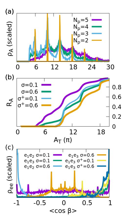
Figure 2: Characterization of the parameters of the optimal protocols found by spatio-temporal control with fidelity higher than $0.999$. In (a) we show the probability distribution of the protocols as a function of the total pulse area for different pulse sequences, $\rho_{A}$. In (b) we show the cumulative distribution $R_{A}$, as a function of the total pulse area, for $3$-pulse sequences at different values of $\sigma$. In (c) we show the distribution of the cosine of the angle between the structural vectors for $3$-pulse sequences using different values of $\sigma$.

We can characterize the optimal solutions in parameter space or in relation to the mechanism (dynamics) that they imply for the gate performance. In Fig.2(a) we represent the scaled distribution of optimal solutions $\rho_{A}(A_{T})={\cal N}_{A}/{\cal N}_{\epsilon}$ as a function of the total pulse area, where ${\cal N}_{\epsilon}$ is the total number of solutions with an error smaller than $\epsilon=10^{-3}$, and ${\cal N}_{A}$ is the subset of those solutions with a total area in the vicinity of $A_{T}=\sum_{k}|A_{k}|$ (within an interval $\Delta A=0.05\pi$). The results are shown for different pulse sequences with $\sigma=0.1$. Two-pulse sequences constrain all possible optimal solutions such that $A_{T}/\pi=6+4l$, $l\in\mathbb{Z}$. The structural vectors must be completely aligned, $\bf{e}_{2}=\bf{e}_{1}$. The effect of the constraints shows up in $A_{T}$, but also in strong correlations in the areas of the two pulses, as shown in Fig.3(a), where we represent the fraction of solutions as a function of $A_{1}$ and $A_{2}$ for the $2$-pulse sequence. The pulse areas must alternate: one following $4l+2$, the other $4l^{\prime}+4$, ($l,l^{\prime}\in\mathbb{Z}$).

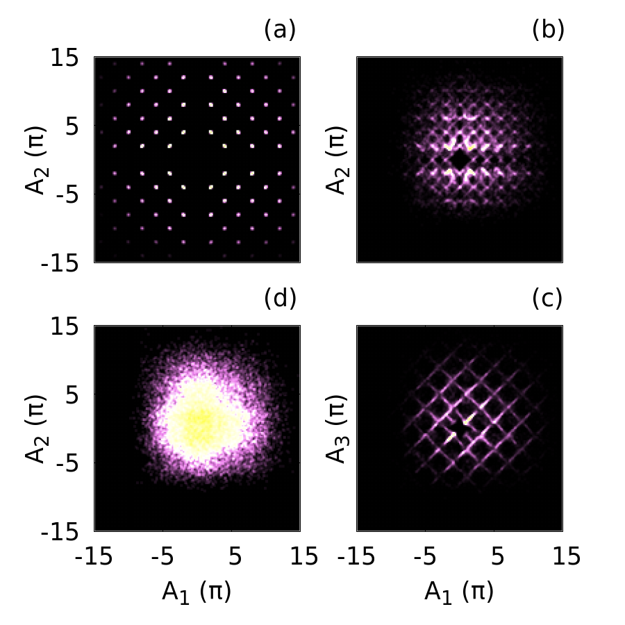
Figure 3: Distribution of the pulse areas for the optimal protocols using (a) 2 pulses, (b) and (c) 3 pulses, (d) 4 pulses. The color scale grading from black to red to yellow indicate the frequency of the observed values. In (c) we choose $A_{3}$ instead of $A_{2}$.

Adding an extra pulse weakens the constraints, so intermediate values of $A_{T}$ become possible. A minimum total pulse area of $4\pi$ is necessary for high fidelity, and particularly for $N_{p}=3$ one can observe maxima at $A_{T}=4\pi$ and $8\pi$. These protocols coincide with the pulse areas in the JP [51] and in the SOP [65]. For this set of solutions, $\langle{\bf e}_{1}|{\bf e}_{2}\rangle=\langle{\bf e}_{2}|{\bf e}_{3}\rangle=0$, while ${\bf e}_{1}={\bf e}_{3}$. However, among the set of all possible solutions with high fidelity, the propensity for these values is small. The distribution of optimal areas changes for different values of $\sigma$ and in p-restricted protocols, especially in short sequences ($N_{p}\leq 3$). Fig.2(b) shows the cumulative distribution of protocols with a total area smaller than $A_{T}$, $R_{A}(A_{T})=\int_{0}^{A_{T}}\rho_{A}(A^{\prime}_{T})dA^{\prime}_{T}$. For $\sigma=0.1$ there are protocols with minimum pulse area $A_{T}\sim 4\pi$. In contrast, p-restricted protocols need $A_{T}\gtrsim 9\pi$. The step-wise behavior clearly reveals that some values of $A_{T}$ are preferred, which differ depending on the setup. It is possible to find protocols that use weaker fields, but at the expense of worsening the fidelity of the gate.

In Fig.2(c) we evaluate the correlation between geometrical vectors for $3$-pulse sequences as a distribution of their relative orientation, $\rho_{ee}(\cos\beta)={\cal N}_{\beta}/{\cal N}_{\epsilon}$, where ${\cal N}_{\beta}$ is the subset of solutions with a corresponding value of $\cos\beta$ (within an interval of $0.05$) and error smaller than $10^{-3}$. With $\sigma=0.1$, ${\bf e}_{1}$ and ${\bf e}_{3}$ are mostly aligned, while ${\bf e}_{2}$ can take any orientation with respect to the previous vectors, with small preferences for aligned, anti-aligned, and at angles $0.23\pi,0.77\pi$, corresponding to $\langle{\bf e}_{1}|{\bf e}_{2}\rangle=\pm 0.75$. Interestingly, with larger $\sigma$, ${\bf e}_{1}$ and ${\bf e}_{2}$ tend to be anti-aligned, while ${\bf e}_{3}$ is mostly oriented perpendicular to the other vectors, with clear peaks in the distribution at $0.42\pi$ and $0.58\pi$ angles. These signatures reveal different underlying mechanisms for the operation of the gate that we believe correlate to 1-loop or 2-loop mechanisms, as we comment in Sec. IV.

Fig.3(b) and (c) show that for $3$-pulse sequences one can still find correlations among the pulse areas, especially between $A_{1}$ and $A_{3}$ (subfigure c). However, for pulse sequences with four or more pulses, almost any value of $A_{T}$ larger than $4\pi$ is possible, although values of $A_{T}/\pi=4l+6$ (not $4l+4$) and aligned or anti-aligned structural vectors (not orthogonal) are still slightly preferred within the set of higher fidelity protocols. The decay at larger values of $A_{T}$ observed in Fig.3 is artificial, due to the imposed range in the sampling of initial parameters. The possible pairwise correlations between the geometrical factors or between other parameters increase with the square of the number of pulses, but at most, weak correlations are observed in the set of all optimal protocols. To analyze the behavior of the different optimal protocols we resort now to the mechanism analysis introduced in Sec.III. By constraining the protocols to obey particular mechanisms, we will show that clearer correlations can be inferred between the optimal parameters.

V Mechanism analysis

Optimal protocols based on $2$-pulse sequences are characterized by highly constrained values for the optimal areas and fully aligned structural vectors. Mechanistically, when starting in the $|00\rangle$ state, these protocols consist solely of pure $0$-loops, resulting in $\left(x^{V},y^{V}\right)=(-1,-1)$. When starting in either the $|01\rangle$ or $|10\rangle$ there can be pure $0$-loops and $1$-loops, as well as collaborative mechanisms that involve contributions of both loops. In such cases, if one dominates when starting in $|01\rangle$, the opposite dominates when starting in $|10\rangle$.

Figure 4: m-square showing the dominance of different mechanisms in optimal protocols for the $V$ subsystem with $3$-pulse sequences (a) to (c); $4$-pulse sequences (d) to (f); $5$-pulse sequences (g) to (i). In the left column $\sigma=0.1$, the center is for p-restrictive protocols with $\sigma^{+}=0.1$ and the right column for $\sigma=0.6$. The last row is reserved for mechanism for the $A$ subsystem with $N_{p}=3$ (j), $4$ (k) and $5$ (l).

Fig.4 gives a panorama of the mechanisms found for the $V$ subsystem. From top to bottom we increase the number of pulses ($N_{p}=3,4,5$), and from left to right the constraints ($\sigma=0.1$, $\sigma^{+}=0.1$, $\sigma=0.6$). Except for the last row, which is dedicated to the mechanisms found in the $A$ subsystem (which are the same as those in the $B$ subsystem) for different pulse sequences ($N_{p}=3,4,5$ from left to right). The frequency of solutions is normalized to the peak value of the distribution, hence a higher density of colors implies a broader set of mechanisms for the optimal protocols.

The most obvious conclusion is the wider choice of mechanisms (and of frequent mechanisms) that shows up with the number of pulses or the strength of the constraints. Focusing on the similarities, for fixed $\sigma$ the m-squares tend to increase the density of solutions towards the center and towards 2-loops, as the number of pulses increases.

For $3$-pulse sequences, the m-square for the $V$ subsystem with $\sigma=0.1$ [Fig.4(a)] shows most mechanisms lying in a triangle, involving mostly pure 0-loops (the dominant mechanism) and collaborative mechanisms mostly at the center of the square. Pure 1-loop mechanisms are very infrequent, but become more important for $\sigma^{+}=0.1$ and especially so for $\sigma=0.6$. In the latter case, the collaborative mechanisms involve mainly 0-loops and 1-loops, rather than d-loops. If we confine the mechanism analysis to the set of protocols with smaller pulse areas ($A_{T}<6\pi$ or $A_{T}<10\pi$ for p-restricted protocols, results not shown in Fig.4) we observe the same tendency: a bigger contribution of d-loops in collaborative mechanisms, as pure mechanisms cease to appear.

The m-square for $4$-pulse sequences is a colorful version of the $3$-pulse case, which brighter features towards the center. While 2-loops are not possible in $3$-pulse sequences, they are available in $4$ and $5$-pulse protocols and become more important as $\sigma$ or the number of pulses increase.

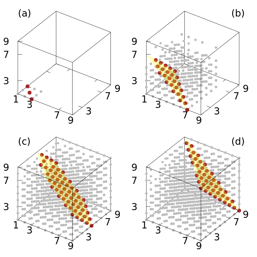
Figure 5: m-cube showing the most frequent mechanisms (brown circles) and all observed mechanisms (gray) used by the optimal protocols with (a) 2-pulses, (b) 3-pulses, (c) 4-pulses and (d) 5-pulse sequences. The most frequent mechanisms occupy planes, shown in yellow.

By symmetry, the m-square for the $A$ and $B$ subsystems is always the same and typically displays a more variety of viable mechanisms than in the $V$ subsystem, with prevalent mechanisms along the diagonal (1-loops to d-loops and their combinations). Pure 0-loops are still possible, but their presence is mostly reduced to 3-pulse sequences. As $N_{p}$ increases, d-loops and 2-loops become more important. For 5-pulse sequences the prevalent mechanisms practically occupy all the upper triangle of the m-square. On the other hand, the diagrams are qualitatively similar regardless of $\sigma$.

But the $(x^{S},y^{S})$ values of the different subsystems are not independent. To better visualize this information, we partitioned the $x$ and $y$ m-square for each subsystem in $9$ boxes and assigned an integer value $\omega^{S}\in[1,9]$ to each mechanism based on the location of the $(x^{S},y^{S})$ coordinates. Hence, for each system, pure or dominant 0-loops correspond to $\omega=1$, 1-loops to $\omega=3$, d-loops to $\omega=7$, and 2-loops to $\omega=9$. Collaborative mechanisms rank between the closest pure mechanisms, or possibly fully collaborative mechanisms ($\omega=5$). We choose the $xy$ plane to represent $\omega^{V}$, the $yz$ plane for $\omega^{A}$ and the $xz$ plane for $\omega^{B}$. The three values of $\omega$ characterize a point in the so-called m-cube, which is shown in Fig.5 for the different pulse sequences with $\sigma=0.1$. The color indicates the probability of finding such a mechanism among the set of optimal protocols with an error smaller than $10^{-3}$. As a reference, Jaksch protocol is a pure d-loop for the $V$ subsystem, a pure 0-loop for the $A$ subsystem, and a pure 1-loop for the $B$ subsystem, occupying the $(1,3,7)$ point in the m-cube.

Fig.5(a) shows that all mechanisms for the $2$-pulse sequences lie in the $xy$ plane ($\omega^{V}=1$), and most of them are in the diagonal, that is, $\omega^{A}+\omega^{B}=4$. Hence, whenever the gate performs as a 0-loop in $A$, it works as a 1-loop in $B$ and vice versa. The same correlation over $\omega^{A}$ and $\omega^{B}$ is observed in $3$-pulse sequences, but in a weaker form. Now the majority of the mechanisms show up with $\omega^{S}\in[1,3]$ or $\omega^{S}=7$, especially in $\omega^{V}$. The m-cube looks similar when we constrain the analysis to high-fidelity protocols (error smaller than $10^{-7}$), so the decay in the rate of success of the algorithms (see Fig.1) has no clear implications from the mechanistic point of view.

While the center of the m-cube is always filled with mechanisms, almost all mechanisms are used as the number of pulses increases. Interestingly, the preferred mechanisms lie on a single plane (shaded in yellow in Fig.5). The value of $\omega_{T}$, which is the sum of the three $\omega$ values ($\omega_{T}=\omega^{V}+\omega^{A}+\omega^{B}$), is equal to $9$ for $3$-pulse sequences, $15$ for $4$-pulse sequences and $21$ for $5$-pulse sequences, when $\sigma=0.1$. This implies a surprising symmetry where the preferred optimal protocols use the same mechanisms regardless of the sub-system where it is applied, as the role of $\omega^{S}$ can be interchanged between the different subsystems. Large values of $\omega_{T}$ mostly correspond to favoring 2-loops over d-loops, and d-loops over 1-loops in the colloborative mechanisms, as one moves from $3$ to $5$-pulse sequences. Similar or slightly lower values are observed for larger $\sigma$.

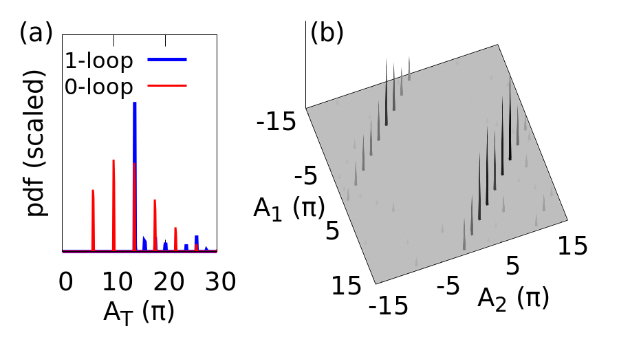
Figure 6: Distribution of the pulse areas of the optimal protocols with error smaller than $0.01$ obtained by optimizing $2$-pulse sequences that use only pure 0-loop or 1-loop mechanisms in the $V$ subsystem. In (b) we show the correlation between the pulse areas in 1-loop mechanisms. The correlation for the 0-loop mechanism is shown in Fig.3.

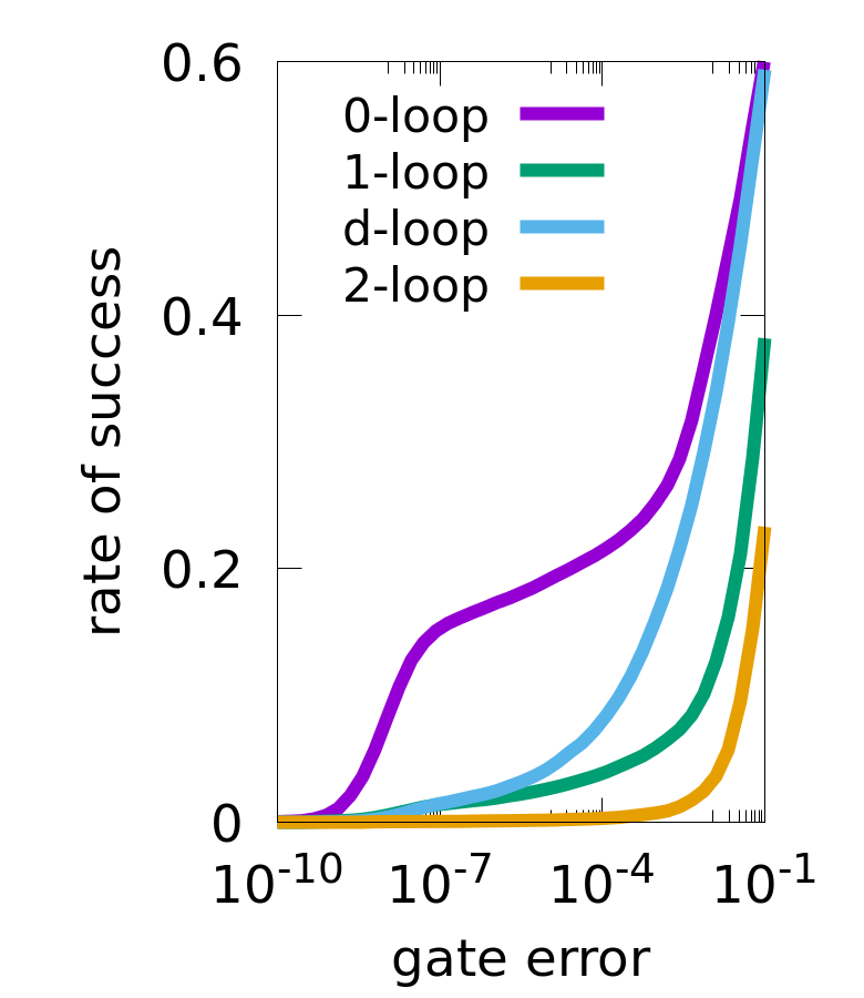
Figure 7: Rate of success as a function of the threshold error, using $4$-pulse sequences to optimize the gate following pre-determined mechanisms.

VI Mechanism-guided optimization

Although the rate of success for finding optimal protocols and the mechanisms they imply increase with the number of pulses, it is interesting to evaluate whether there are other optimal protocols that are not being found by the optimization algorithm. The density of solutions in parameter space suggests that the algorithm tends to find protocols that are close to the initial conditions. Repeating the optimization from different sets of initial conditions produces similar results. Very symmetric protocols occupy a negligible volume in parameter space and typically have lower fidelities, so one needs to impose the symmetries as restrictions in the optimization algorithm to find them [65].

In this work, we follow a different procedure to find optimal protocols by maximizing the fidelity evaluated with the chosen pathways, thus finding mechanism-driven protocols of our choice. In the following, we constrain the optimization to obtain pure mechanisms in the $V$ subsystem, while the gate may perform differently in the other subsystems, thus selecting a specific family of mechanisms. Using this procedure it is possible to find previously unexplored protocols even under highly-constraining conditions. For instance, we can find pure 1-loop protocols in 2-pulse sequences with fidelity better than $F\geq 0.99$ (but not better than $0.999$). Fig.6 shows how the pulse areas are now correlated, following a very different pattern than in 0-loop protocols. The correlation between $A_{1}$ and $A_{2}$ differs and $A_{T}$ has different values than before and is typically larger. Although most protocols imply aligned structural vectors, anti-aligned vectors are also possible.

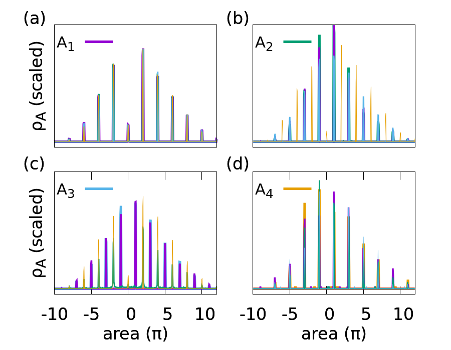
Figure 8: Time-domain features of the optimization. Distribution of the pulse areas $A_{1}$ (violet), $A_{2}$ (green), $A_{3}$ (blue), $A_{4}$ (orange) for the optimal protocols that use only (a) 0-loops, (b) 1-loops, (c) d-loops, and (d) 2-loops in the $V$ subsystem.

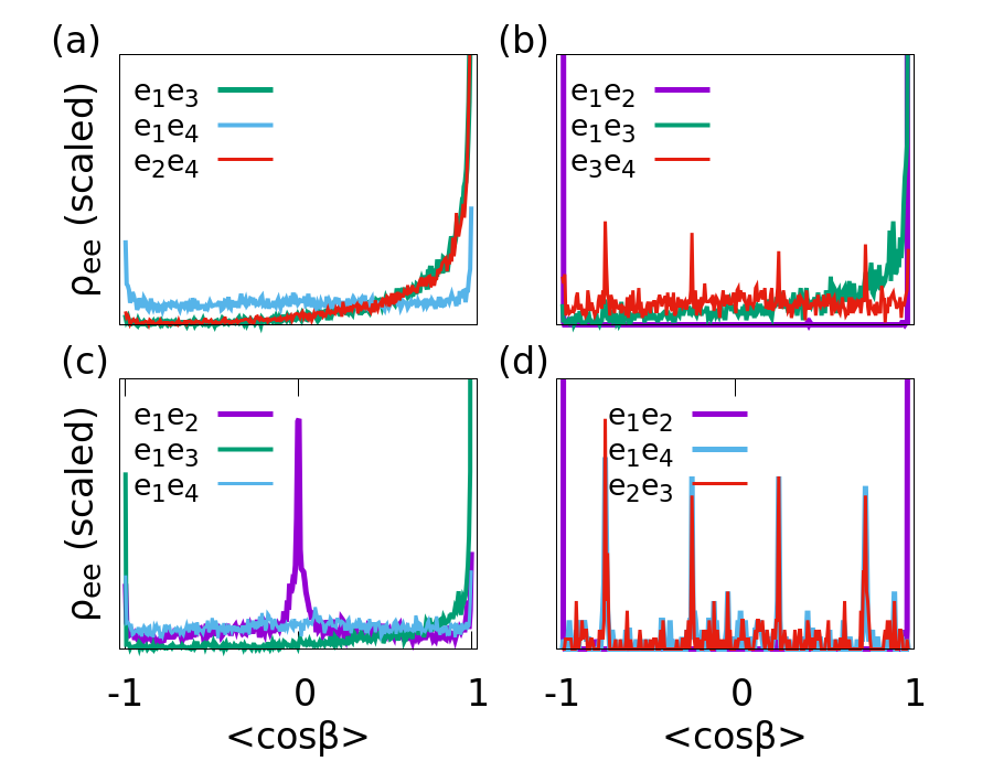
Figure 9: Spatial-domain features of the optimization. Distribution of the cosine of the angles between structural vectors for the optimal protocols that only use (a) 0-loops, (b) 1-loops, (c) d-loops, and (d) 2-loops in the $V$ subsystem.

In Fig.7 we show the rate of success of the optimization at selecting protocols in $4$-pulse sequences. As expected from our previous analysis without mechanism selection, pure 0-loops are easy to find even in gates performing at high-fidelity. Lowest fidelity protocols are achieved by pure 2-loop protocols, hence their absence in the unconstrained optimizations.

Fig.8 shows the distribution of pulse areas for the different mechanisms, and Fig.9 some representative correlations between structural vectors. Protocols with pure-mechanisms constrain the pulse areas such that in 0-loops and 2-loops all pulses have the same areas; in 1-loops, the areas of the fourth pulses $A_{4}$ differ, and in d-loops odd pulses and even pulses have different areas. The total pulse areas in 0-loop protocols follow the same rules as in the 2-pulse sequences: $A_{T}/\pi=6+4l$. In all other cases, the rule is $A_{T}/\pi=6+2l$ except in d-loops, which also allow total pulse areas smaller than $6\pi$. In average, pure 0-loop and 2-loop protocols typically require larger $A_{T}$ than 1-loop and d-loop protocols. Collaborative mechanisms can further reduce the pulse areas.

The analysis of the vector correlations shows the following: In 0-loop protocols, odd vectors (${\bf e}_{1},{\bf e}_{3}$) as well as even vectors (${\bf e}_{2},{\bf e}_{4}$) are mostly aligned with each other, while odd to even vectors show up at any possible orientation, with some preference for aligned or anti-aligned configurations. In 1-loop protocols, ${\bf e}_{1}$ and ${\bf e}_{3}$ are strictly aligned or anti-aligned to ${\bf e}_{2}$, while they are mostly aligned to each other; ${\bf e}_{4}$ appears at all possible orientations but the distribution shows peaks at $0.23\pi,0.42\pi,0.58\pi$ and $0.77\pi$, corresponding to $\langle{\bf e}_{4}|{\bf e}_{j}\rangle=\pm 0.25,\pm 0.75$. In d-loop protocols, ${\bf e}_{1}$ and ${\bf e}_{3}$ are both strictly aligned or anti-aligned to each other, and perpendicular to ${\bf e}_{2}$, while ${\bf e}_{4}$ takes all possible orientations. Finally, in 2-loops ${\bf e}_{1}$ is aligned or anti-aligned to ${\bf e}_{2}$, and ${\bf e}_{3}$ to ${\bf e}_{4}$, while ${\bf e}_{3}$ and ${\bf e}_{4}$ show at $0.23\pi,0.42\pi,0.58\pi$ and $0.77\pi$ angles with respect to both ${\bf e}_{1}$ and ${\bf e}_{2}$.

VII Summary and Conclusions

Using quantum control tools, we have explored the space of optimal protocols for implementing CZ entangling gates in systems of two non-independent qubits, with high fidelity. Studying the rate of success of the optimal control algorithm as a function of the gate error for different pulse sequences under different constraints, we have evaluated the impact of the proximity of the atoms. High fidelity protocols can be found already with $2$-pulse sequences in highly interdependent qubits, where each field acts strongly on both qubits at the same time. However, the density of solutions decreases as the qubits approach each other, and in a more pronounced way if the fields are forced to be positive everywhere. The minimal pulse areas necessary to implement the protocols also increase with the constraints.

To characterize the protocols up to $5$-pulse sequences, we have proposed a mechanism analysis based on pathways that connect the initial computational state of the qubit with the final state, in terms of 0-, 1-, d-, and 2-loops, represented on a square. We have approximately ranked the solutions in terms of pure mechanisms or their combinations, characterizing each protocol by a point in a cube. Finally, we have developed optimization algorithms that select protocols that operate under chosen mechanisms.

All protocols in 2-pulse sequences require a 0-loop mechanism for the dynamics starting in $|00\rangle$ (for the dynamics starting in $|01\rangle$ or $|10\rangle$ the mechanism can be a 0 or 1-loop or its superposition). But lower-fidelity protocols can be found forcing a 1-loop mechanism in $|00\rangle$, at the expense of needing larger pulse areas. The correlations in the parameters are not obvious for longer pulse sequences but can be found by imposing mechanism constraints. For instance, $4$-pulse sequences that implement pure mechanisms inherit much of the structure of $2$-pulse sequences. Some mechanisms involve preferred orientations in the structural vectors and probably reveal interesting Hamiltonian structures that are exploited in the gate dynamics, in the same way that the SOP used a dark state [65].

While for large pulse sequences almost any possible mechanisms is used by different optimal protocols, the set of preferred mechanisms lie on a single plane, revealing that strong correlations also characterize the space of mechanisms. These correlations are such that for any dominant mechanism, by interchanging the type of controlled dynamics starting in any computational basis of the qubit (except the uncoupled $|11\rangle$ state), one can find an alternative dominant optimal protocol. As the number of pulses increases, or the constraints become stronger, collaborative mechanisms are favored where the largest contributions move from 0-loops to 1-loops, from 1-loops to d-loops, and from d-loops to 2-loops. The mechanisms for the dynamics starting from the $|01\rangle$ or the $|10\rangle$ states are typically more varied than those starting from $|00\rangle$, but less dependent on the constraints.

From the theoretical point of view, our study offers a novel methodology to map and characterize a dense space of optimal protocols of general validity for quantum computing, regardless of the gate or specific platform. To date, most proposed quantum protocols were based on human ingenuity, forcing very restricting sets of parameters. These highly symmetrical protocols typically implied gates that operated with pure mechanisms. However, in the full space of mechanisms, such protocols can only be found by guiding the search, biasing the optimization algorithm. At the expense of increasing the complexity of the system, controlling the spatial properties of the laser beams working with structured light, we have shown in this work that the landscape of protocols is much richer than expected, and exploring this landscape offers great flexibility for the experimental implementation.

References

- Cirac and Zoller [2000] J. I. Cirac and P. Zoller, A scalable quantum computer with ions in an array of microtraps, Nature 404, 579 (2000).
- Ladd et al. [2010] T. D. Ladd, F. Jelezko, R. Laflamme, Y. Nakamura, C. Monroe, and J. L. O’Brien, Quantum computers, Nature 464, 45 (2010).
- Devoret and Schoelkopf [2013] M. H. Devoret and R. J. Schoelkopf, Superconducting circuits for quantum information: An outlook, Science 339, 1169 (2013).
- Kelly et al. [2015] J. Kelly, R. Barends, A. G. Fowler, A. Megrant, E. Jeffrey, T. C. White, D. Sank, J. Y. Mutus, B. Campbell, Y. Chen, Z. Chen, B. Chiaro, A. Dunsworth, I.-C. Hoi, C. Neill, P. J. J. O’Malley, C. Quintana, P. Roushan, A. Vainsencher, J. Wenner, A. N. Cleland, and J. M. Martinis, State preservation by repetitive error detection in a superconducting quantum circuit, Nature 519, 66 (2015).
- Harty et al. [2014] T. P. Harty, D. T. C. Allcock, C. J. Ballance, L. Guidoni, H. A. Janacek, N. M. Linke, D. N. Stacey, and D. M. Lucas, High-fidelity preparation, gates, memory, and readout of a trapped-ion quantum bit, Phys. Rev. Lett. 113, 220501 (2014).
- Jelezko et al. [2004] F. Jelezko, T. Gaebel, I. Popa, M. Domhan, A. Gruber, and J. Wrachtrup, Observation of coherent oscillation of a single nuclear spin and realization of a two-qubit conditional quantum gate, Phys. Rev. Lett. 93, 130501 (2004).
- Saffman et al. [2010] M. Saffman, T. G. Walker, and K. Mølmer, Quantum information with rydberg atoms, Rev. Mod. Phys. 82, 2313 (2010).
- Zhu et al. [2022] D. Zhu, Z. P. Cian, C. Noel, A. Risinger, D. Biswas, L. Egan, Y. Zhu, A. M. Green, C. H. Alderete, N. H. Nguyen, Q. Wang, A. Maksymov, Y. Nam, M. Cetina, N. M. Linke, M. Hafezi, and C. Monroe, Cross-platform comparison of arbitrary quantum states, Nature Communications 13, 6620 (2022).
- Rice and Zhao [2000] S. Rice and M. Zhao, Optical Control of Molecular Dynamics (John Wiley & Sons, Ltd, 2000).
- Shapiro and Brummer [2011] M. Shapiro and P. Brummer, Quantum Control of Molecular Processes (John Wiley & Sons, Ltd, 2011).
- Shore [2011] B. W. Shore, Manipulating Quantum Structures Using Laser Pulses (Cambridge University Press, 2011).
- Malinovsky and Sola [2004a] V. S. Malinovsky and I. R. Sola, Quantum control of entanglement by phase manipulation of time-delayed pulse sequences. i, Phys. Rev. A 70, 042304 (2004a).
- Malinovsky and Sola [2004b] V. S. Malinovsky and I. R. Sola, Quantum phase control of entanglement, Phys. Rev. Lett. 93, 190502 (2004b).
- Malinovsky and Sola [2006] V. S. Malinovsky and I. R. Sola, Phase-controlled collapse and revival of entanglement of two interacting qubits, Phys. Rev. Lett. 96, 050502 (2006).
- Palao and Kosloff [2003] J. P. Palao and R. Kosloff, Optimal control theory for unitary transformations, Phys. Rev. A 68, 062308 (2003).
- Tesch et al. [2001] C. M. Tesch, L. Kurtz, and R. de Vivie-Riedle, Applying optimal control theory for elements of quantum computation in molecular systems, Chemical Physics Letters 343, 633 (2001).
- Tesch and de Vivie-Riedle [2002] C. M. Tesch and R. de Vivie-Riedle, Quantum computation with vibrationally excited molecules, Phys. Rev. Lett. 89, 157901 (2002).
- Palao et al. [2008] J. P. Palao, R. Kosloff, and C. P. Koch, Protecting coherence in optimal control theory: State-dependent constraint approach, Phys. Rev. A 77, 063412 (2008).
- Goerz et al. [2014] M. H. Goerz, D. M. Reich, and C. P. Koch, Optimal control theory for a unitary operation under dissipative evolution, New Journal of Physics 16, 055012 (2014).
- Caneva et al. [2011] T. Caneva, T. Calarco, and S. Montangero, Chopped random-basis quantum optimization, Phys. Rev. A 84, 022326 (2011).
- Glaser et al. [2015] S. J. Glaser, U. Boscain, T. Calarco, C. P. Koch, W. Köckenberger, R. Kosloff, I. Kuprov, B. Luy, S. Schirmer, T. Schulte-Herbrüggen, D. Sugny, and F. K. Wilhelm, Training schrödinger’s cat: quantum optimal control, The European Physical Journal D 69, 279 (2015).
- Koch et al. [2022] C. P. Koch, U. Boscain, T. Calarco, G. Dirr, S. Filipp, S. J. Glaser, R. Kosloff, S. Montangero, T. Schulte-Herbrüggen, D. Sugny, and F. K. Wilhelm, Quantum optimal control in quantum technologies. strategic report on current status, visions and goals for research in europe, EPJ Quantum Technology 9, 19 (2022).
- Müller et al. [2011] M. M. Müller, D. M. Reich, M. Murphy, H. Yuan, J. Vala, K. B. Whaley, T. Calarco, and C. P. Koch, Optimizing entangling quantum gates for physical systems, Phys. Rev. A 84, 042315 (2011).
- Theis et al. [2016] L. S. Theis, F. Motzoi, F. K. Wilhelm, and M. Saffman, High-fidelity rydberg-blockade entangling gate using shaped, analytic pulses, Phys. Rev. A 94, 032306 (2016).
- Rabitz et al. [2004] H. A. Rabitz, M. M. Hsieh, and C. M. Rosenthal, Quantum optimally controlled transition landscapes, Science 303, 1998 (2004).
- Rothman et al. [2006] A. Rothman, T.-S. Ho, and H. Rabitz, Exploring the level sets of quantum control landscapes, Phys. Rev. A 73, 053401 (2006).
- Chakrabarti and Rabitz [2007] R. Chakrabarti and H. Rabitz, Quantum control landscapes, International Reviews in Physical Chemistry 26, 671 (2007).
- Palao et al. [2013] J. P. Palao, D. M. Reich, and C. P. Koch, Steering the optimization pathway in the control landscape using constraints, Phys. Rev. A 88, 053409 (2013).
- Pechen and Tannor [2011] A. N. Pechen and D. J. Tannor, Are there traps in quantum control landscapes?, Phys. Rev. Lett. 106, 120402 (2011).
- Ho et al. [2009] T.-S. Ho, J. Dominy, and H. Rabitz, Landscape of unitary transformations in controlled quantum dynamics, Phys. Rev. A 79, 013422 (2009).
- Moore and Rabitz [2012] K. W. Moore and H. Rabitz, Exploring constrained quantum control landscapes, The Journal of Chemical Physics 137, 134113 (2012).
- Russell et al. [2017] B. Russell, H. Rabitz, and R.-B. Wu, Control landscapes are almost always trap free: a geometric assessment, Journal of Physics A: Mathematical and Theoretical 50, 205302 (2017).
- Nogrette et al. [2014] F. Nogrette, H. Labuhn, S. Ravets, D. Barredo, L. Béguin, A. Vernier, T. Lahaye, and A. Browaeys, Single-atom trapping in holographic 2d arrays of microtraps with arbitrary geometries, Phys. Rev. X 4, 021034 (2014).
- Barredo et al. [2016] D. Barredo, S. de Léséleuc, V. Lienhard, T. Lahaye, and A. Browaeys, An atom-by-atom assembler of defect-free arbitrary two-dimensional atomic arrays, Science 354, 1021 (2016).
- Wilson et al. [2022] J. T. Wilson, S. Saskin, Y. Meng, S. Ma, R. Dilip, A. P. Burgers, and J. D. Thompson, Trapping alkaline earth rydberg atoms optical tweezer arrays, Phys. Rev. Lett. 128, 033201 (2022).
- Burgers et al. [2022] A. P. Burgers, S. Ma, S. Saskin, J. Wilson, M. A. Alarcón, C. H. Greene, and J. D. Thompson, Controlling rydberg excitations using ion-core transitions in alkaline-earth atom-tweezer arrays, PRX Quantum 3, 020326 (2022).
- Lee et al. [2016] W. Lee, H. Kim, and J. Ahn, Three-dimensional rearrangement of single atoms using actively controlled optical microtraps, Opt. Express 24, 9816 (2016).
- Comparat and Pillet [2010] D. Comparat and P. Pillet, Dipole blockade in a cold rydberg atomic sample, J. Opt. Soc. Am. B 27, A208 (2010).
- Tong et al. [2004] D. Tong, S. M. Farooqi, J. Stanojevic, S. Krishnan, Y. P. Zhang, R. Côté, E. E. Eyler, and P. L. Gould, Local blockade of rydberg excitation in an ultracold gas, Phys. Rev. Lett. 93, 063001 (2004).
- Urban et al. [2009a] E. Urban, T. A. Johnson, T. Henage, L. Isenhower, D. D. Yavuz, T. G. Walker, and M. Saffman, Observation of rydberg blockade between two atoms, Nature Physics 5, 110 (2009a).
- Gaëtan et al. [2009] A. Gaëtan, Y. Miroshnychenko, T. Wilk, A. Chotia, M. Viteau, D. Comparat, P. Pillet, A. Browaeys, and P. Grangier, Observation of collective excitation of two individual atoms in the rydberg blockade regime, Nature Physics 5, 115 (2009).
- Pritchard et al. [2010] J. D. Pritchard, D. Maxwell, A. Gauguet, K. J. Weatherill, M. P. A. Jones, and C. S. Adams, Cooperative atom-light interaction in a blockaded rydberg ensemble, Phys. Rev. Lett. 105, 193603 (2010).
- Levine et al. [2018] H. Levine, A. Keesling, A. Omran, H. Bernien, S. Schwartz, A. S. Zibrov, M. Endres, M. Greiner, V. Vuletić, and M. D. Lukin, High-fidelity control and entanglement of rydberg-atom qubits, Phys. Rev. Lett. 121, 123603 (2018).
- Zeng et al. [2017] Y. Zeng, P. Xu, X. He, Y. Liu, M. Liu, J. Wang, D. J. Papoular, G. V. Shlyapnikov, and M. Zhan, Entangling two individual atoms of different isotopes via rydberg blockade, Phys. Rev. Lett. 119, 160502 (2017).
- Jo et al. [2020] H. Jo, Y. Song, M. Kim, and J. Ahn, Rydberg atom entanglements in the weak coupling regime, Phys. Rev. Lett. 124, 033603 (2020).
- Wilk et al. [2010] T. Wilk, A. Gaëtan, C. Evellin, J. Wolters, Y. Miroshnychenko, P. Grangier, and A. Browaeys, Entanglement of two individual neutral atoms using rydberg blockade, Phys. Rev. Lett. 104, 010502 (2010).
- Graham et al. [2022] T. M. Graham, Y. Song, J. Scott, C. Poole, L. Phuttitarn, K. Jooya, P. Eichler, X. Jiang, A. Marra, B. Grinkemeyer, M. Kwon, M. Ebert, J. Cherek, M. T. Lichtman, M. Gillette, J. Gilbert, D. Bowman, T. Ballance, C. Campbell, E. D. Dahl, O. Crawford, N. S. Blunt, B. Rogers, T. Noel, and M. Saffman, Multi-qubit entanglement and algorithms on a neutral-atom quantum computer, Nature 604, 457 (2022).
- Maller et al. [2015] K. M. Maller, M. T. Lichtman, T. Xia, Y. Sun, M. J. Piotrowicz, A. W. Carr, L. Isenhower, and M. Saffman, Rydberg-blockade controlled-not gate and entanglement in a two-dimensional array of neutral-atom qubits, Phys. Rev. A 92, 022336 (2015).
- Zhang et al. [2010] X. L. Zhang, L. Isenhower, A. T. Gill, T. G. Walker, and M. Saffman, Deterministic entanglement of two neutral atoms via rydberg blockade, Phys. Rev. A 82, 030306 (2010).
- Picken et al. [2018] C. J. Picken, R. Legaie, K. McDonnell, and J. D. Pritchard, Entanglement of neutral-atom qubits with long ground-rydberg coherence times, Quantum Science and Technology 4, 015011 (2018).
- Jaksch et al. [2000] D. Jaksch, J. I. Cirac, P. Zoller, S. L. Rolston, R. Côté, and M. D. Lukin, Fast quantum gates for neutral atoms, Phys. Rev. Lett. 85, 2208 (2000).
- Isenhower et al. [2011] L. Isenhower, M. Saffman, and K. Mølmer, Multibit cknot quantum gates via rydberg blockade, Quantum Information Processing 10, 755 (2011).
- Lukin et al. [2001] M. D. Lukin, M. Fleischhauer, R. Cote, L. M. Duan, D. Jaksch, J. I. Cirac, and P. Zoller, Dipole blockade and quantum information processing in mesoscopic atomic ensembles, Phys. Rev. Lett. 87, 037901 (2001).
- Levine et al. [2019] H. Levine, A. Keesling, G. Semeghini, A. Omran, T. T. Wang, S. Ebadi, H. Bernien, M. Greiner, V. Vuletić, H. Pichler, and M. D. Lukin, Parallel implementation of high-fidelity multiqubit gates with neutral atoms, Phys. Rev. Lett. 123, 170503 (2019).
- Cohen and Thompson [2021] S. R. Cohen and J. D. Thompson, Quantum computing with circular rydberg atoms, PRX Quantum 2, 030322 (2021).
- Shi [2022] X.-F. Shi, Quantum logic and entanglement by neutral rydberg atoms: methods and fidelity, Quantum Science and Technology 7, 023002 (2022).
- Shi [2018] X.-F. Shi, Deutsch, toffoli, and cnot gates via rydberg blockade of neutral atoms, Phys. Rev. Applied 9, 051001 (2018).
- Paredes-Barato and Adams [2014] D. Paredes-Barato and C. S. Adams, All-optical quantum information processing using rydberg gates, Phys. Rev. Lett. 112, 040501 (2014).
- Adams et al. [2019] C. S. Adams, J. D. Pritchard, and J. P. Shaffer, Rydberg atom quantum technologies, Journal of Physics B: Atomic, Molecular and Optical Physics 53, 012002 (2019).
- Malinovsky et al. [2014] V. S. Malinovsky, I. R. Sola, and J. Vala, Phase-controlled two-qubit quantum gates, Phys. Rev. A 89, 032301 (2014).
- Goerz et al. [2011] M. H. Goerz, T. Calarco, and C. P. Koch, The quantum speed limit of optimal controlled phasegates for trapped neutral atoms, Journal of Physics B: Atomic, Molecular and Optical Physics 44, 154011 (2011).
- Morgado and Whitlock [2021] M. Morgado and S. Whitlock, Quantum simulation and computing with rydberg-interacting qubits, AVS Quantum Science 3, 10.1116/5.0036562 (2021), cited by: 56; All Open Access, Green Open Access.
- Young et al. [2021] J. T. Young, P. Bienias, R. Belyansky, A. M. Kaufman, and A. V. Gorshkov, Asymmetric blockade and multiqubit gates via dipole-dipole interactions, Phys. Rev. Lett. 127, 120501 (2021).
- Saffman et al. [2020] M. Saffman, I. I. Beterov, A. Dalal, E. J. Páez, and B. C. Sanders, Symmetric rydberg controlled- gates with adiabatic pulses, Phys. Rev. A 101, 062309 (2020).
- Sola et al. [2023] I. R. Sola, V. S. Malinovsky, J. Ahn, S. Shin, and B. Y. Chang, Two-qubit atomic gates: spatio-temporal control of rydberg interaction, Nanoscale 15, 4325 (2023).
- Murty [1964] M. V. R. K. Murty, A simple way of demonstrating the phase reversals in the tem10, tem20, tem30 modes of a gas laser source, Appl. Opt. 3, 1192 (1964).
- Forbes et al. [2021] A. Forbes, M. de Oliveira, and M. R. Dennis, Structured light, Nature Photonics 15, 253 (2021).
- Rubinsztein-Dunlop et al. [2016] H. Rubinsztein-Dunlop, A. Forbes, M. V. Berry, M. R. Dennis, D. L. Andrews, M. Mansuripur, C. Denz, C. Alpmann, P. Banzer, T. Bauer, E. Karimi, L. Marrucci, M. Padgett, M. Ritsch-Marte, N. M. Litchinitser, N. P. Bigelow, C. Rosales-Guzmán, A. Belmonte, J. P. Torres, T. W. Neely, M. Baker, R. Gordon, A. B. Stilgoe, J. Romero, A. G. White, R. Fickler, A. E. Willner, G. Xie, B. McMorran, and A. M. Weiner, Roadmap on structured light, Journal of Optics 19, 013001 (2016).
- Šibalić and Adams [2018] N. Šibalić and C. S. Adams, Rydberg Physics, 2399-2891 (IOP Publishing, 2018).
- Gallagher [1994] T. F. Gallagher, Rydberg Atoms, Cambridge Monographs on Atomic, Molecular and Chemical Physics (Cambridge University Press, 1994).
- Urban et al. [2009b] E. Urban, T. A. Johnson, T. Henage, L. Isenhower, D. D. Yavuz, T. G. Walker, and M. Saffman, Observation of rydberg blockade between two atoms, Nature Physics 5, 110 (2009b).
- Scotto [2016] S. Scotto, Rubidium vapors in high magnetic fields, Ph.D. thesis (2016).
- Chew et al. [2022] Y. Chew, T. Tomita, T. P. Mahesh, S. Sugawa, S. de Léséleuc, and K. Ohmori, Ultrafast energy exchange between two single rydberg atoms on a nanosecond timescale, Nature Photonics 16, 724 – 729 (2022).
- Nielsen and Chuang [2010] M. A. Nielsen and I. L. Chuang, Quantum Computation and Quantum Information: 10th Anniversary Edition (Cambridge University Press, 2010).
- [75] P. R. Berman and V. S. Malinovsky, Principles of Laser Spectroscopy and Quantum Optics (Princeton University Press, 2011).
- [76] I. R. Sola, B. Y. Chang, S. A. Malinovskaya, and V. S. Malinovsky, Advances In Atomic, Molecular, and Optical Physics, Vol. 67, edited by E. Arimondo, L. F. DiMauro, and S. F. Yelin (Academic Press, 2018) pp. 151-256.
- Nelder and Mead [1965] J. A. Nelder and R. Mead, A Simplex Method for Function Minimization, The Computer Journal 7, 308 (1965), https://academic.oup.com/comjnl/article-pdf/7/4/308/1013182/7-4-308.pdf .
- Powell [1998] M. J. D. Powell, Direct search algorithms for optimization calculations, Acta Numerica 7, 287–336 (1998).