Isometric tensor network optimization for extensive Hamiltonians is free of barren plateaus

Abstract

We explain why and numerically confirm that there are no barren plateaus in the energy optimization of isometric tensor network states (TNS) for extensive Hamiltonians with finite-range interactions. Specifically, we consider matrix product states, tree tensor network states, and the multiscale entanglement renormalization ansatz. The variance of the energy gradient, evaluated by taking the Haar average over the TNS tensors, has a leading system-size independent term and decreases according to a power law in the bond dimension. For a hierarchical TNS with branching ratio $b$, the variance of the gradient with respect to a tensor in layer $\tau$ scales as $(b\eta)^{\tau}$, where $\eta$ is the second largest eigenvalue of the Haar-average doubled layer-transition channel and decreases algebraically with increasing bond dimension. The observed scaling properties of the gradient variance bear implications for efficient initialization procedures.

I Introduction

The rapid recent advances in quantum technology have opened new routes for the solution of hard quantum groundstate problems. Well-controlled quantum devices are a natural platform for the investigation of complex quantum matter Feynman1982-21 . A popular approach are variational quantum algorithms (VQA) Cerezo2021-9 , in which classical optimization is performed on parametrized quantum circuits. Numerous studies have successfully applied VQA to few-body systems. However, applications of generic unstructured VQA to many-body systems face multiple challenges: (a) Current quantum hardware is limited in the available number of qubits and gate fidelities. (b) As with other high-dimensional nonlinear optimization problems, we are typically confronted with complex cost-function landscapes and it is difficult to avoid local minima Kiani2020_01 ; Bittel2021-127 ; Anschuetz2021_09 ; Anschuetz2022-13 . (c) In contrast to classical computers, the quantum algorithms produce a sequence of probabilistic measurement results for gradients, requiring a large number of shots to achieve precise estimates. For a generic unstructured VQA, gradient amplitudes decay exponentially in the size of the simulated system McClean2018-9 ; Cerezo2021-12 . This is the so-called barren plateau problem. In this case, VQA are not trainable as the inability to precisely estimate exponentially small gradients will result in random walks on the flat landscape. The barren plateau problem can be resolved if an initial guess close to the optimum and good optimization strategies are available Grant2019-3 ; Zhang2022_03 ; Mele2022_06 ; Kulshrestha2022_04 ; Dborin2022-7 ; Skolik2021-3 ; Slattery2022-4 ; Haug2021_04 ; Sack2022-3 ; Rad2022_03 ; Tao2022_05 , but such resolutions are not universal Campos2021-103 .

Unstructured circuits like the hardware efficient ansatz and brickwall circuits must be deep in order to cover relevant parts of the Hilbert space Dankert2009-80 ; Brandao2016-346 ; Harrow2018_09 . The high expressiveness of such circuits Sim2019-2 ; Nakaji2021-5 ; Du2022-128 can be seen as the source for the barren plateaus Holmes2022-3 . The latter can also be motivated by the typicality properties Goldstein2006-96 ; Popescu2006-2 of such states Ortiz2021-2 ; Patti2021-3 ; Sharma2022-128 . So, it is generally preferable to work with more structured and less entangled classes of states that are adapted to the particular optimization problem in order to balance expressiveness and trainability.

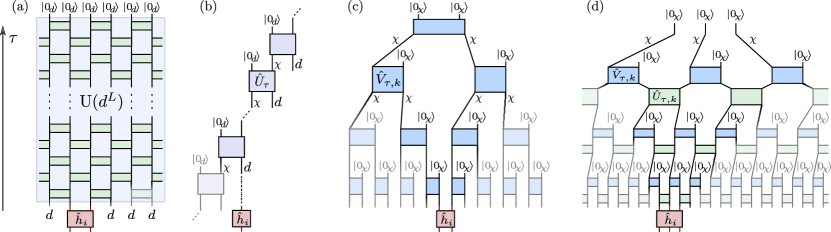
Figure 1: Isometric quantum circuits. (a) A generic brickwall quantum circuit for $L$ qudits. (b) MPS quantum circuit with single-site Hilbert space dimension $d$ and bond dimension $\chi$. (c,d) Binary 1D TTNS and MERA quantum circuits with branching ratio $b=2$ and bond dimension $\chi$. The non-shaded tensors compose the causal-cone states $|\Psi_{i}\rangle$ associated with local operators $\hat{h}_{i}$.

In this work, we show that VQA barren plateaus can be avoided for quantum many-body ground state problems by employing matrix product states (MPS) Baxter1968-9 ; Accardi1981 ; Fannes1992-144 ; White1992-11 ; Rommer1997 ; PerezGarcia2007-7 ; Schollwoeck2011-326 , tree tensor network states (TTNS) Fannes1992-66 ; Otsuka1996-53 ; Shi2006-74 ; Murg2010-82 ; Tagliacozzo2009-80 , or the multiscale entanglement renormalization ansatz (MERA) Vidal-2005-12 ; Vidal2006 ; Barthel2010-105 . The entanglement structure of these isometric tensor network states (TNS) is well-adapted to the one in many-body ground states. Variations of such isometric TNS can be implemented on quantum computers Liu2019-1 ; Miao2021_08 ; FossFeig2021-3 ; Niu2022-3 ; Slattery2021_08 which may allows us to substantially reduce computation costs in comparison to classical simulations Miao2021_08 ; Miao2023_03 . Recently, the issue of barren plateaus has been studied for certain randomly initialized TNS using graph techniques Liu2022-129 ; Garcia2023-2023 and ZX-calculus Zhao2021-5 ; Martin2023-7 in the energy optimization for few-site product operators. Of course, the latter are actually solved by product states composed of the single-site ground states and, hence, of rather restricted practical relevance.

Here, we address the groundstate problem for extensive translation-invariant Hamiltonians

$$\textstyle\hat{H}=\sum_{i}\hat{h}_{i}\quad\text{with}\quad\operatorname{Tr}\hat{h}_{i}=0$$ (1)

encountered in quantum many-body physics, where the finite-range interaction term $\hat{h}_{i}$ acts non-trivially around site $i$. We show that the corresponding VQA based on isometric TNS does not encounter barren plateaus. The key ideas are the following: Due to the isometry constraints, the TNS expectation value for a local interaction term $\hat{h}_{i}$ only depends on a reduced causal-cone state. The expectation values can be evaluated by propagating causal-cone density operators ${\hat{\rho}}$ in the preparation direction (decreasing $\tau$ in Fig. 1) with transition maps $\mathcal{M}$ and/or interaction terms $\hat{h}$ in the renormalization direction (increasing $\tau$) with $\mathcal{M}^{\dagger}$. To evaluate the variance of the energy gradient for TNS sampled according to the Haar measure, doubled transition quantum channels $\mathcal{E}^{(2)}:=\operatorname{Avg}\mathcal{M}\otimes\mathcal{M}$ are applied to ${\hat{\rho}}\otimes{\hat{\rho}}$ and their adjoints $\mathcal{E}^{(2){\dagger}}$ to $\hat{h}\otimes\hat{h}$. While the image of ${\hat{\rho}}\otimes{\hat{\rho}}$ will quickly converge to a unique steady state, we find that the leading contribution from $\hat{h}\otimes\hat{h}$ has a decay factor $\propto(b\eta)^{\tau}$, where $\eta$ denotes the second largest eigenvalue of $\mathcal{E}^{(2)}$ and $b$ the branching ratio of the TNS ($b=1$ for MPS). This leads to three key observations: for random isometric TNS and extensive local Hamiltonians, (i) the gradient variance is independent of the total system size rather than exponentially small, (ii) the gradient variance for a tensor in layer $\tau$ of hierarchical TNS decays exponentially in the layer index $\tau$, (iii) the gradient variances decrease according to power laws in the TNS bond dimension $\chi$. Instead of Euclidean gradients in parametrized quantum circuits, we employ Riemannian gradients which greatly simplifies the proofs.

II Riemannian TNS gradients

All tensors in the considered isometric TNS are either unitaries $\hat{U}$ or partial isometries $\hat{V}:\mathbb{C}^{N_{1}}\to\mathbb{C}^{N_{1}}\otimes\mathbb{C}^{N_{2}}$ that we can implement as partially projected unitaries in the form

$$\hat{V}=\hat{U}\,(\mathbbm{1}_{N_{1}}\otimes|0_{N_{2}}\rangle)$$ (2)

with an arbitrary reference state $|0_{N_{2}}\rangle\in\mathbb{C}^{N_{2}}$. The TNS energy expectation values can be written in the form

$$E(\hat{U})=\langle\Psi(\hat{U})|\hat{H}|\Psi(\hat{U})\rangle=\operatorname{Tr}(\hat{X}\tilde{U}^{\dagger}\hat{Y}\tilde{U}),$$ (3)

where we explicitly denote the dependence on one of the TNS unitaries $\hat{U}\in\operatorname{U}(N)$ and $\tilde{U}:=\hat{U}\otimes\mathbbm{1}_{M}$. The Hermitian operators $\hat{X}$ and $\hat{Y}$ depend on the other TNS tensors and $\hat{Y}$ also comprises the Hamiltonian. The Riemannian energy gradient is then given by Hauru2021-10 ; Luchnikov2021-23 ; Miao2021_08 ; Wiersema2022_02 ; Barthel2023_03

$$\hat{g}(\hat{U})=\partial_{\hat{U}}\langle\Psi|\hat{H}|\Psi\rangle=\operatorname{Tr}_{M}(\hat{Y}\tilde{U}\hat{X}-\tilde{U}\hat{X}\tilde{U}^{\dagger}\hat{Y}\tilde{U}).$$ (4)

Averaged according to the Haar measure, $\hat{g}$ vanishes,

$$\textstyle\operatorname{Avg}_{\hat{U}}\hat{g}:=\int\mathrm{d}U\,\hat{g}(\hat{U})=\frac{1}{2}\int\mathrm{d}U[\hat{g}(\hat{U})+\hat{g}(-\hat{U})]=0.$$

In order to assess the question of barren plateaus, the Haar variance of the Riemannian gradient (4) can be quantified by

$$\textstyle\operatorname{Var}_{\hat{U}}\hat{g}:=\operatorname{Avg}_{\hat{U}}\frac{1}{N}\operatorname{Tr}(\hat{g}^{\dagger}\hat{g}).$$ (5)

We can expand $\hat{g}$ in an orthonormal basis of $N^{2}$ Hermitian and unitary operators $\{\hat{\sigma}_{n}\}$ with $\hat{\sigma}_{n}^{2}=\mathbbm{1}_{N}$ such that $\hat{g}=\mathrm{i}\hat{U}\sum_{n=1}^{N^{2}}\alpha_{n}\hat{\sigma}_{n}/N$. On a quantum computer, the rotation-angle derivatives can be determined as energy differences $\alpha_{n}=E(\hat{U}\mathrm{e}^{{\mathrm{i}\pi\hat{\sigma}_{n}}/{4}})-E(\hat{U}\mathrm{e}^{{-\mathrm{i}\pi\hat{\sigma}_{n}}/{4}})$ Miao2021_08 ; Wiersema2022_02 . Equation (5) then agrees with the variance $\int\mathrm{d}U\,\frac{1}{N^{2}}\sum_{n}\alpha_{n}^{2}$, motivating the employed factor $1/N$.

We focus on the extensive Hamiltonians (1) with finite-range interactions $\hat{h}_{i}$. Let $j$ denote the position of a unitary tensor $\hat{U}_{j}$ in the TNS and $\mathcal{S}_{j}$ the set of physical sites $i$ with $\hat{U}_{j}$ in the causal cone; cf. Fig. 1. The gradient (4) then takes the form

$$\textstyle\hat{g}(\hat{U}_{j})=\sum_{i\in\mathcal{S}_{j}}\hat{g}^{(i)}_{j}\quad\text{with}\quad\hat{g}^{(i)}_{j}:=\partial_{\hat{U}_{j}}\langle\Psi|\hat{h}_{i}|\Psi\rangle$$

Averaging over all unitaries of the TNS, the Haar variance of $\hat{g}(\hat{U}_{j})$ reads

$$\textstyle\operatorname{Var}\hat{g}(\hat{U}_{j})=\sum_{i_{1},i_{2}\in\mathcal{S}_{j}}\operatorname{Avg}\,\frac{1}{N}\operatorname{Tr}\big{(}\hat{g}_{j}^{(i_{1}){\dagger}}\hat{g}_{j}^{(i_{2})}\big{)}.$$ (6)

III Matrix product states

Consider MPS of bond dimension $\chi$ for a system of $L$ sites and single-site dimension $d$,

$$|\Psi\rangle=\!\!\sum_{s_{1},\dotsc,s_{L}=1}^{d}\!\!\langle 0|\hat{V}_{1}^{s_{1}}\hat{V}_{2}^{s_{2}}\dotsb\hat{V}_{L}^{s_{L}}|0\rangle\,|s_{1},s_{2},\dotsc,s_{L}\rangle.$$ (7)

Using its gauge freedom, the MPS can be brought to left-orthonormal form Schollwoeck2011-326 , where the tensors $\hat{V}_{j}$ with $\langle a,s|\hat{V}_{j}|b\rangle:=\langle a|\hat{V}^{s_{j}}|b\rangle$ and $a,b=1,\dotsc,\chi$ are isometries in the sense that $\hat{V}_{j}^{\dagger}\hat{V}_{j}=\mathbbm{1}_{\chi}$. We use Eq. (2) to express them in terms of unitaries with $\hat{V}_{j}=:\hat{U}_{j}\,(\mathbbm{1}_{\chi}\otimes|0_{d}\rangle)$ in the bulk of the system such that $\hat{U}_{j}\in\operatorname{U}(\chi\,d)$ Barthel2023_03 .

Let us first address Hamiltonians (1) with single-site terms $\hat{h}_{i}=\mathbbm{1}_{d}^{\otimes(i-1)}\otimes\hat{h}\otimes\mathbbm{1}_{d}^{\otimes(L-i)}$. Due to the left-orthonormality, the local expectation value $\langle\Psi|\hat{h}_{i}|\Psi\rangle$ is independent of all tensors $\hat{U}_{j}$ with $j<i$ such that $\mathcal{S}_{j}=\{1,\dotsc,j\}$. As we chose $\operatorname{Tr}\hat{h}_{i}=0$ without loss of generality, all off-diagonal contributions with $i_{1}\neq i_{2}$ in Eq. (6) vanish. It remains to evaluate the diagonal contributions with $i_{1}=i_{2}=i\leq j$: The expectation value has the form (3). In particular,

$$\langle\Psi|\hat{h}_{i} |\Psi\rangle=\operatorname{Tr}(\hat{X}_{j}^{(i)}\hat{U}_{j}^{\dagger}\hat{Y}_{j}^{(i)}\hat{U}_{j})\quad\text{with}$$ (8a)

$$\hat{X}_{j}^{(i)} =\mathcal{M}_{j+1}\circ\dotsb\circ\mathcal{M}_{L}(|0\rangle\langle 0|)\otimes|0_{d}\rangle\langle 0_{d}|\ \ \text{and}$$ (8b)

$$\hat{Y}_{j}^{(i)} =\mathcal{M}^{\dagger}_{j-1}\circ\dotsb\circ\mathcal{M}^{\dagger}_{i+1}(\hat{L}^{(i)})\otimes\mathbbm{1}_{d},\quad$$ (8c)

where $\hat{L}^{(i)}=\hat{V}_{i}^{\dagger}[\mathbbm{1}_{\chi}\otimes\hat{h}\big{]}\hat{V}_{i}$, and we have defined the site-transition map

$$\textstyle\mathcal{M}_{\tau}(\hat{R}):=\sum_{s}\hat{V}^{s}_{\tau}\hat{R}\hat{V}^{s{\dagger}}_{\tau}.$$

According to Eq. (4), the contribution $\operatorname{Avg}\operatorname{Tr}\big{(}\hat{g}_{j}^{(i){\dagger}}\hat{g}_{j}^{(i)}\big{)}$ to the gradient variance (6) is quadratic in both $\hat{X}_{j}^{(i)}$ and $\hat{Y}_{j}^{(i)}$. The essential step is hence to evaluate the Haar averages $\operatorname{Avg}\hat{X}_{j}^{(i)}\otimes\hat{X}_{j}^{(i)}$ and $\operatorname{Avg}\hat{Y}_{j}^{(i)}\otimes\hat{Y}_{j}^{(i)}$, i.e.,

$$\operatorname{Avg}\mathcal{M}^{\otimes 2}_{j+1}\circ\dotsb\circ\mathcal{M}^{\otimes 2}_{L}(|0,0\rangle\langle 0,0|)\quad\text{and}$$ (9)

$$\operatorname{Avg}\mathcal{M}^{{\dagger}\otimes 2}_{j-1}\circ\dotsb\circ\mathcal{M}^{{\dagger}\otimes 2}_{i+1}(\hat{L}^{(i)}\otimes\hat{L}^{(i)}).$$ (10)

Taking the Haar averages over the involved unitaries $\hat{U}_{\tau}$, yields the doubled site-transition channel

$$\mathcal{E}_{\text{mps}}^{(2)}:=\operatorname{Avg}_{\hat{U}_{\tau}}\mathcal{M}^{\otimes 2}_{\tau}=|\hat{r}_{1}\rangle\!\rangle\langle\!\langle\mathbbm{1}_{\chi^{2}}|+\eta_{\text{mps}}\,|\hat{r}_{2}\rangle\!\rangle\langle\!\langle\hat{\ell}_{2}|.$$ (11)

Here, we have already written its diagonalized form, using a super-bra-ket notation for operators based on the Hilbert-Schmidt inner product $\langle\!\langle\hat{A}|\hat{B}\rangle\!\rangle:=\operatorname{Tr}(\hat{A}^{\dagger}\hat{B})$. The diagonalization, as detailed in the companion paper Barthel2023_03 , shows that $\mathcal{E}_{\text{mps}}^{(2)}$ has a unique steady state $\hat{r}_{1}$ and first excitation $\hat{r}_{2}$ with the eigenvalue $\eta_{\text{mps}}=\frac{1-1/\chi^{2}}{d-1/(\chi^{2}d)}$. The repeated application of $\mathcal{E}_{\text{mps}}^{(2)}$ in Eq. (9) quickly converges to $\hat{r}_{1}$. Similarly, its application in Eq. (10) would converge to the corresponding left eigenoperator $\mathbbm{1}_{\chi^{2}}$, but one finds that this does not contribute to the gradient variance. It is the subleading term $\propto\eta_{\text{mps}}^{j-i}\hat{\ell}_{2}$ that ultimately yields

$$\frac{\operatorname{Avg}\operatorname{Tr}\big{(}\hat{g}_{j}^{(i){\dagger}}\hat{g}_{j}^{(i)}\big{)}}{\chi\,d}=\frac{2\operatorname{Tr}(\hat{h}^{2})}{d(\chi^{2}d+1)}\,\eta_{\text{mps}}^{j-i}+\mathcal{O}(\eta_{\text{mps}}^{L-i}).$$ (12)

Finally, the variance (6) for the extensive Hamiltonian is obtained by summing the contributions (12) for all $i\leq j$, resulting in the system-size independent value

$$2\operatorname{Tr}(\hat{h}^{2})\frac{\chi^{2}d^{2}-1}{d(d-1)(\chi^{2}d+1)^{2}}+\mathcal{O}(\eta_{\text{mps}}^{j})+\mathcal{O}(\eta_{\text{mps}}^{L-j}),$$ (13)

where the sub-leading terms are due to boundary effects.

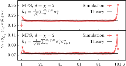
Figure 2: MPS gradient variance. For spin-1/2 chains (1) of length $L=101$ with single-site terms $\hat{h}_{i}$ (upper panel) and nearest-neighbor interactions (lower panel), we plot the gradient variance (6) for the tensor at site $j$. Numerical averages over 64 000 MPS with tensors sampled according to the Haar measure agree with the analytical result (13).

The optimization problem with single-site terms $\hat{h}_{i}$ is trivially solved by product states but, qualitatively, things do not change for finite-range interactions $\hat{h}_{i}$. The second largest eigenvalue $\eta_{\text{mps}}$ of the doubled transition channel (11), remains the most important quantity. A detailed analysis is given in the companion paper Barthel2023_03 . Figure 2 confirms the analytical prediction in numerical tests. MPS optimizations have no barren plateaus for extensive Hamiltonians.

IV Hierarchical TNS

MERA Vidal-2005-12 ; Vidal2006 ; Barthel2010-105 are hierarchical TNS. Starting on $\mathcal{N}$ sites, in each renormalization step $\tau\to\tau+1$, we apply local unitary disentanglers $\hat{U}_{\tau,k}$ of layer $\tau$ before the number of degrees of freedom is reduced by applying isometries $\hat{V}_{\tau,k}$ that map groups of $b$ sites into one renormalized site. The associated site dimension $\chi$ is the bond dimension and $b$ is the so-called branching ratio. The process stops at the top layer $\tau=T$ by projecting each of the remaining $\mathcal{N}/b^{T}$ sites onto a reference state $|0_{\chi}\rangle$. The renormalization procedure, seen in reverse, generates the MERA $|\Psi\rangle$. TTNS Fannes1992-66 ; Otsuka1996-53 ; Shi2006-74 ; Murg2010-82 ; Tagliacozzo2009-80 are a subclass of MERA without disentanglers.

As all tensors are isometric, the evaluation of local expectation values drastically simplifies, where $\langle\Psi|\hat{h}_{i}|\Psi\rangle$ only depends on the tensors in the causal cone of $\hat{h}_{i}$. See Fig. 1. In fact, the expectation value can again be written in a form very similar to Eq. (8) but, now, we have transition maps $\mathcal{M}_{\tau,i}$ that map the causal-cone density operator ${\hat{\rho}}_{\tau}$ into ${\hat{\rho}}_{\tau-1}=\mathcal{M}_{\tau,i}({\hat{\rho}}_{\tau})$.

Specifically, for the binary one-dimensional (1D) MERA in Fig. 1d and a three-site interaction term $\hat{h}_{i}$, we start in the top layer with the three-site reference state ${\hat{\rho}}_{T}=(|0_{\chi}\rangle\langle 0_{\chi}|)^{\otimes 3}$ and then progress down layer by layer, applying either a left-moving or a right-moving transition map $\mathcal{M}_{\tau,i}$. These consist in applying three isometries that double the number of (renormalized) sites, then applying two disentanglers and, finally, tracing out one site on the left and two on the right (left-moving) or vice versa (right-moving). The diagonal contributions to the gradient variance for $\hat{U}_{\tau,k}$ with $i_{1}=i_{2}=i$ in Eq. (6), are functions of $\operatorname{Avg}\hat{X}_{\tau,k}^{(i)}\otimes\hat{X}_{\tau,k}^{(i)}$ and $\operatorname{Avg}\hat{Y}_{\tau,k}^{(i)}\otimes\hat{Y}_{\tau,k}^{(i)}$, where label $j$ has been replaced by a layer number $\tau$ and renormalized site $k$ in that layer. Taking the Haar average of $\mathcal{M}_{t,i}^{\otimes 2}$, we obtain either a left-moving or a right-moving doubled layer-transition channel $\mathcal{E}^{(2)}_{\text{bi},\text{L}}$ and $\mathcal{E}^{(2)}_{\text{bi},\text{R}}$. Summing over all sites $i\in\mathcal{S}_{\tau,k}$ that have $\hat{U}_{\tau,k}$ in their causal cone, corresponds to summing over all possible sequences of the two channels. This is equivalent to applying the map $2\mathcal{E}^{(2)}_{\text{bi}}$ for layers $t=1,\dotsc,\tau-1$, where

$$\mathcal{E}^{(2)}_{\text{bi}}:=\frac{1}{2}\left(\mathcal{E}^{(2)}_{\text{bi},\text{L}}+\mathcal{E}^{(2)}_{\text{bi},\text{R}}\right)$$ (14)

is the average transition channel. Finally, averaging the gradient variance $\operatorname{Var}\hat{g}(\hat{U}_{\tau,k})$ with respect to $k$ in layer $\tau$ corresponds to applying $\mathcal{E}^{(2)}_{\text{bi}}$ for all layers $t=\tau+1,\dotsc,T$.

The channel $\mathcal{E}^{(2)}_{\text{bi}}$ is diagonalizable and gapped,

$$\textstyle\mathcal{E}^{(2)}_{\text{bi}}=|\hat{r}_{1}\rangle\!\rangle\langle\!\langle\hat{\ell}_{1}|+\sum_{n=2}^{4}\lambda_{n}|\hat{r}_{n}\rangle\!\rangle\langle\!\langle\hat{\ell}_{n}|\ \ \text{with}$$ (15)

$$\textstyle\hat{\ell}_{1}=\mathbbm{1}_{\chi^{6}},\ \ \eta_{\text{bi}}:=\lambda_{2}=\frac{\chi^{2}(1+\chi)^{4}}{2(1+\chi^{2})^{4}},\ \ \lambda_{3}=\frac{\chi^{2}(1+\chi)^{2}}{2(1+\chi^{2})^{3}},$$

biorthogonal left and right eigenvectors $\langle\!\langle\hat{\ell}_{n}|\hat{r}_{n^{\prime}}\rangle\!\rangle=\delta_{n,n^{\prime}}$, and $\frac{1}{2}>\lambda_{2}>\lambda_{3}>\lambda_{4}$. Similar to the analysis for MPS, the leading term in $\operatorname{Avg}\hat{X}_{\tau,k}^{(i)}\otimes\hat{X}_{\tau,k}^{(i)}$ stems from the $\mathcal{E}^{(2)}_{\text{bi}}$ steady state $\hat{r}_{1}$, while the leading term in $\operatorname{Avg}\hat{Y}_{\tau,k}^{(i)}\otimes\hat{X}_{\tau,k}^{(i)}$ stems from the first excitation $\hat{\ell}_{2}$. In this way, one finds that the diagonal contributions to the gradient variance $\operatorname{Var}\partial_{\hat{U}_{\tau,k}}\langle\Psi|\hat{H}|\Psi\rangle$ [Eq. (6)], averaged for all $k$ in layer $\tau$, scale as

$$\operatorname{Var}\hat{g}(\hat{U}_{\tau})=\Theta((2\eta_{\text{bi}})^{\tau})+\mathcal{O}((2\lambda_{3})^{\tau})+\mathcal{O}(2^{\tau}\eta_{\text{bi}}^{T}),$$ (16)

where the Landau symbol $\Theta(f)$ indicates that there exist upper and lower bounds scaling like $f$. The off-diagonal terms with $|i_{1}-i_{2}|>3$ vanish due to $\operatorname{Tr}\hat{h}_{i}=0$ and the remaining off-diagonal terms have the same scaling as the diagonal terms. See Ref. Barthel2023_03 for details.

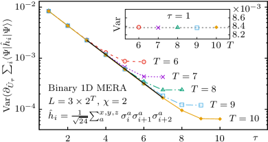
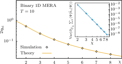
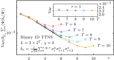
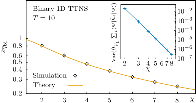
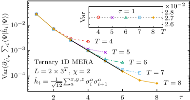
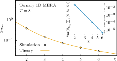
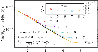
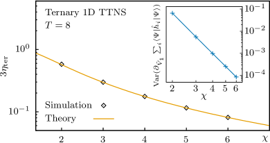
Figure 3: Gradient variance in heterogeneous 1D MERA and TTNS. In the hierarchical isometric TNS, the leading term in the Haar-variance of the energy gradient is system-size independent and decreases exponentially in the layer index $\tau$. The graphs on left show this exponential decay observed in numerical tests for bond dimension $\chi=2$. Black lines indicate the fitting range for the decay factors. The inserts show the gradient variance at $\tau=1$ as a function of the number of layers $T$, corresponding to varying system size $L=b^{T}$. The graphs on the right show a perfect agreement of the decay factors, extracted from simulations for various bond dimensions $\chi$, and the theoretical prediction $b\eta$. The inserts assert the power-law decay of gradient variances in layer $\tau=1$ with respect to $\chi$. For simplicity, we choose the physical single-site dimensions as $d=\chi$ and Hamiltonians $\hat{H}=\sum_{i=1}^{L}\hat{h}_{i}$ with normalized two or three-site interactions $\hat{h}_{i}$ constructed from generalized Gell-Mann matrices according to Eq. (17).

The analysis for the binary 1D MERA can be extended to all MERA and TTNS. The central object in the evaluation of their Haar-averaged gradient variances are doubled layer-transition channels $\mathcal{E}^{(2)}$. The gradient variance for tensors in layer $\tau$ will then scale as $(b\eta)^{\tau}$, where $\eta$ is the second largest $\mathcal{E}^{(2)}$ eigenvalue. This eigenvalue decreases algebraically with increasing bond dimension $\chi$ such that $b\eta<1$ for $\chi>1$. Specifically, we find $\eta=\chi/(1+\chi^{2})$ for binary 1D TTNS, $\eta=1/(3\chi^{2})+\mathcal{O}(\chi^{-4})$ for ternary 1D MERA, $\eta=\chi^{2}/(1+\chi^{2}+\chi^{4})$ for ternary 1D TTNS, and $\eta=1/(9\chi^{8})+\mathcal{O}(\chi^{-10})$ for the 2D $3\times 3\mapsto 1$ MERA Evenbly2009-79 . So, for each layer $\tau$, the gradient variance is an algebraic function of the bond dimension $\chi$ and (up to corrections) independent of the total system size. Therefore, the optimization of hierarchical TNS is not hampered by barren plateaus.

For the 1D TNS, these analytical results are tested and confirmed numerically as shown in Fig. 3. For the numerical tests, we choose the physical single-site dimension $d$ equal to the bond dimension $\chi$. Otherwise, one would use the lowest MERA layers to increase bond dimensions gradually from $d$ to the desired $\chi$. The isotropic interaction terms $\hat{h}_{i}$ are constructed using generalized $\chi\times\chi$ Gell-Mann matrices $\{\hat{\Lambda}^{1},\hat{\Lambda}^{2},\cdots,\hat{\Lambda}^{\chi^{2}-1}\}$ Kimura2003-314 ; Bertlmann2008-41 . They are traceless and Hermitian generalizations of the Pauli matrices $\hat{\sigma}^{a}$ for $\chi=2$ and the Gell-Mann matrices for $\chi=3$. As generators of the special unitary group SU$(\chi)$, they satisfy the orthonormality condition $\langle\!\langle\hat{\Lambda}^{a}|\hat{\Lambda}^{b}\rangle\!\rangle=2\delta_{a,b}$. We define $n$-site interactions as

$$\textstyle\hat{h}_{i}=\frac{1}{\sqrt{2^{n}(\chi^{2}-1)}}\sum_{a=1}^{\chi^{2}-1}\hat{\Lambda}^{a}_{i}\otimes\dotsb\otimes\hat{\Lambda}^{a}_{i+n-1},$$ (17)

which are traceless, have vanishing partial traces, and are normalized according to $\operatorname{Tr}(\hat{h}_{i}^{2})=1$. Each data point in Fig. 3 corresponds to 1000 TNS with tensors sampled according the Haar measure. The numerical results confirm the scaling $(b\eta)^{\tau}$ with corrections at small $\tau$ and due to the finite number of layers $T$. The extracted decay factors $b\eta$ show the predicted $\chi$ dependence. As a numerically sampling of 2D MERA and TTNS is computationally expensive, a direct extraction of decay factors from sampled gradient variances is currently not possible for 2D.

V Homogeneous and Trotterized MERA and TTNS

So far, we have exclusively considered heterogeneous TNS, where all tensors can vary freely. To save computational resources, one can also work with homogeneous TNS where, in the case of MERA and TTNS, all equivalent disentanglers and isometries of a given layer $\tau$ are chosen to be identical. Such homogeneous TNS can also be used to initialized the optimization of heterogeneous TNS. The theoretical analysis of gradient variances for homogeneous TNS is more involved. While the analysis for heterogeneous TNS only requires first and second-moment Haar-measure integrals, more complicated higher-order integrals are needed for the homogeneous states. Hence, we determine the gradient variance for homogeneous TTNS and MERA numerically as shown in Fig. 4, finding that homogeneous TNS have considerably larger gradient variances than the corresponding heterogeneous states. This is consistent with findings in Refs. Volkoff2021-6 ; Pesah2021-11 for other classes of states.

Isometric TNS can be implemented on quantum computers, but it is advisable to impose a substructure for the TNS tensors to reduce costs and achieve a quantum advantage. Specifically, in Trotterized MERA Miao2021_08 ; Miao2023_03 ; Kim2017_11 , each tensor is constructed as brickwall circuit with $t$ (Trotter) steps. A generic full MERA can be recovered by increasing $t$. Fig. 4 compares gradient variances for homogeneous Trotterized MERA and full MERA as well as those for Trotterized and full TTNS. The data shows that Trotterized TNS have larger gradients variances than full TNS, and the former converge to the latter as $t$ increases.

VI Discussion

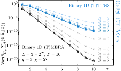
Figure 4: Gradient variances for homogeneous Trotterized TNS. For the model (17), the plot shows the gradient variances at layer $\tau$ for homogeneous binary 1D Trotterized TTNS (blue dashed lines), full TTNS (blue full line), Trotterized MERA (gray dashed lines) and full MERA (black full line).

The presented results suggest that isometric TNS generally feature no barren plateaus in the energy optimization for extensive models with finite-range interactions. It should be rather straightforward to generalize to systems with $k$-local interactions. The observed scaling of the gradient variance has implications for efficient initialization schemes: For MPS, the power-law decay in the bond dimension $\chi$ suggests to start with an optimization at small $\chi$ and to then gradually increase it. For TTNS and MERA, the exponential decay in the layer index $\tau$, suggests that iteratively increasing the number of layers during optimization can substantially improve the performance. TTNS have considerably larger gradient variances than MERA. For MERA optimizations, it can hence be beneficial to initially choose all disentanglers as identities and only start their optimization after the corresponding TTNS has converged.

The analysis in Ref. Kim2017_11 suggests that VQA based on hierarchical TNS is robust with respect to noise in the quantum devices. A natural extension of our analysis would be to study the doubled transition channels with environment fluctuations. We expect that no noise-induced barren plateaus Wang2021-12 ; Wiersema2021_11 occur for TNS.

The methods employed in this work could also be applied to study statistical properties and typicality for random TNS Garnerone2010-81 ; Garnerone2010-82 ; Haferkamp2021-2 , as well as the dynamics of quantum information and entanglement in structured random quantum circuits Nahum2017-7 ; Nahum2018-8 ; Zhou2019-99 ; Potter2022-211 ; Fisher2022_07 .

The absence of barren plateaus in the discussed isometric TNS does not depend on the choice of Riemannian gradients over Euclidean gradients. However, in our practical experience, the parametrization-free Riemannian optimization as described in Ref. Miao2021_08 has better convergence properties and can mitigate some effects of spurious local minima observed for parametrized quantum circuits You2021-139 ; Anschuetz2022-13 ; Liu2022_06 . Further research on this issues is needed.

- (1) R. P. Feynman, Simulating physics with computers, Int. J. Theor. Phys. 21, 467 (1982).
- (2) M. Cerezo, A. Arrasmith, R. Babbush, S. C. Benjamin, S. Endo, K. Fujii, J. R. McClean, K. Mitarai, X. Yuan, L. Cincio, and P. J. Coles, Variational quantum algorithms, Nat. Rev. Phys. 3, 625 (2021).
- (3) B. T. Kiani, S. Lloyd, and R. Maity, Learning unitaries by gradient descent, arXiv:2001.11897 (2020).
- (4) L. Bittel and M. Kliesch, Training variational quantum algorithms is NP-hard, Phys. Rev. Lett. 127, 120502 (2021).
- (5) E. R. Anschuetz, Critical points in quantum generative models, arXiv:2109.06957 (2021).
- (6) E. R. Anschuetz and B. T. Kiani, Quantum variational algorithms are swamped with traps, Nature Commun. 13, 7760 (2022).
- (7) J. R. McClean, S. Boixo, V. N. Smelyanskiy, R. Babbush, and H. Neven, Barren plateaus in quantum neural network training landscapes, Nat. Commun. 9, 4812 (2018).
- (8) M. Cerezo, A. Sone, T. Volkoff, L. Cincio, and P. J. Coles, Cost function dependent barren plateaus in shallow parametrized quantum circuits, Nat. Commun. 12, 1791 (2021).
- (9) E. Grant, L. Wossnig, M. Ostaszewski, and M. Benedetti, An initialization strategy for addressing barren plateaus in parametrized quantum circuits, Quantum 3, 214 (2019).
- (10) K. Zhang, M.-H. Hsieh, L. Liu, and D. Tao, Gaussian initializations help deep variational quantum circuits escape from the barren plateau, arXiv:2203.09376 (2022).
- (11) A. A. Mele, G. B. Mbeng, G. E. Santoro, M. Collura, and P. Torta, Avoiding barren plateaus via transferability of smooth solutions in Hamiltonian Variational Ansatz, arxiv:2206.01982 (2022).
- (12) A. Kulshrestha and I. Safro, BEINIT: Avoiding Barren Plateaus in Variational Quantum Algorithms, arXiv:2204.13751 (2022).
- (13) J. Dborin, F. Barratt, V. Wimalaweera, L. Wright, and A. G. Green, Matrix product state pre-training for quantum machine learning, Quant. Sci. Tech. 7, 035014 (2022).
- (14) A. Skolik, J. R. McClean, M. Mohseni, P. van der Smagt, and M. Leib, Layerwise learning for quantum neural networks, Quantum Mach. Intell. 3, 5 (2021).
- (15) L. Slattery, B. Villalonga, and B. K. Clark, Unitary block optimization for variational quantum algorithms, Phys. Rev. Research 4, 023072 (2022).
- (16) T. Haug and M. Kim, Optimal training of variational quantum algorithms without barren plateaus, arXiv:2104.14543 (2021).
- (17) S. H. Sack, R. A. Medina, A. A. Michailidis, R. Kueng, and M. Serbyn, Avoiding barren plateaus using classical shadows, PRX Quantum 3, 020365 (2022).
- (18) A. Rad, A. Seif, and N. M. Linke, Surviving the barren plateau in variational quantum circuits with Bayesian learning initialization, arXiv:2203.02464 (2022).
- (19) Z. Tao, J. Wu, Q. Xia, and Q. Li, LAWS: Look around and warm-start natural gradient descent for quantum neural networks, arXiv:2205.02666 (2022).
- (20) E. Campos, A. Nasrallah, and J. Biamonte, Abrupt transitions in variational quantum circuit training, Phys. Rev. A 103, 032607 (2021).
- (21) C. Dankert, R. Cleve, J. Emerson, and E. Livine, Exact and approximate unitary 2-designs and their application to fidelity estimation, Phys. Rev. A 80, 012304 (2009).
- (22) F. G. S. L. Brandão, A. W. Harrow, and M. Horodecki, Local random quantum circuits are approximate polynomial-designs, Commun. Math. Phys. 346, 397 (2016).
- (23) A. Harrow and S. Mehraban, Approximate unitary -designs by short random quantum circuits using nearest-neighbor and long-range gates, arXiv:1809.06957 (2018).
- (24) S. Sim, P. D. Johnson, and A. Aspuru-Guzik, Expressibility and entangling capability of parameterized quantum circuits for hybrid quantum-classical algorithms, Adv. Quantum Technol. 2, 1900070 (2019).
- (25) K. Nakaji and N. Yamamoto, Expressibility of the alternating layered ansatz for quantum computation, Quantum 5, 434 (2021).
- (26) Y. Du, Z. Tu, X. Yuan, and D. Tao, Efficient measure for the expressivity of variational quantum algorithms, Phys. Rev. Lett. 128, 080506 (2022).
- (27) Z. Holmes, K. Sharma, M. Cerezo, and P. J. Coles, Connecting ansatz expressibility to gradient magnitudes and barren plateaus, PRX Quantum 3, 010313 (2022).
- (28) S. Goldstein, J. L. Lebowitz, R. Tumulka, and N. Zanghì, Canonical typicality, Phys. Rev. Lett. 96, 050403 (2006).
- (29) S. Popescu, A. J. Short, and A. Winter, Entanglement and the foundations of statistical mechanics, Nat. Phys. 2, 754 (2006).
- (30) C. Ortiz Marrero, M. Kieferová, and N. Wiebe, Entanglement-induced barren plateaus, PRX Quantum 2, 040316 (2021).
- (31) T. L. Patti, K. Najafi, X. Gao, and S. F. Yelin, Entanglement devised barren plateau mitigation, Phys. Rev. Research 3, 033090 (2021).
- (32) K. Sharma, M. Cerezo, L. Cincio, and P. J. Coles, Trainability of dissipative perceptron-based quantum neural networks, Phys. Rev. Lett. 128, 180505 (2022).
- (33) R. J. Baxter, Dimers on a rectangular lattice, J. Math. Phys. 9, 650 (1968).
- (34) L. Accardi, Topics in quantum probability, Phys. Rep. 77, 169 (1981).
- (35) M. Fannes, B. Nachtergaele, and R. F. Werner, Finitely correlated states on quantum spin chains, Commun. Math. Phys. 144, 443 (1992).
- (36) S. R. White, Density matrix formulation for quantum renormalization groups, Phys. Rev. Lett. 69, 2863 (1992).
- (37) S. Rommer and S. Östlund, A class of ansatz wave functions for 1D spin systems and their relation to DMRG, Phys. Rev. B 55, 2164 (1997).
- (38) D. Perez-Garcia, F. Verstraete, M. M. Wolf, and J. I. Cirac, Matrix product state representations, Quantum Info. Comput. 7, 401 (2007).
- (39) U. Schollwöck, The density-matrix renormalization group in the age of matrix product states, Ann. Phys. 326, 96 (2011).
- (40) M. Fannes, B. Nachtergaele, and R. F. Werner, Ground states of VBS models on cayley trees, J. Stat. Phys. 66, 939 (1992).
- (41) H. Otsuka, Density-matrix renormalization-group study of the spin- antiferromagnet on the Bethe lattice, Phys. Rev. B 53, 14004 (1996).
- (42) Y.-Y. Shi, L.-M. Duan, and G. Vidal, Classical simulation of quantum many-body systems with a tree tensor network, Phys. Rev. A 74, 022320 (2006).
- (43) V. Murg, F. Verstraete, O. Legeza, and R. M. Noack, Simulating strongly correlated quantum systems with tree tensor networks, Phys. Rev. B 82, 205105 (2010).
- (44) L. Tagliacozzo, G. Evenbly, and G. Vidal, Simulation of two-dimensional quantum systems using a tree tensor network that exploits the entropic area law, Phys. Rev. B 80, 235127 (2009).
- (45) G. Vidal, Entanglement renormalization, Phys. Rev. Lett. 99, 220405 (2007).
- (46) G. Vidal, Class of quantum many-body states that can be efficiently simulated, Phys. Rev. Lett. 101, 110501 (2008).
- (47) T. Barthel, M. Kliesch, and J. Eisert, Real-space renormalization yields finitely correlated states, Phys. Rev. Lett. 105, 010502 (2010).
- (48) J.-G. Liu, Y.-H. Zhang, Y. Wan, and L. Wang, Variational quantum eigensolver with fewer qubits, Phys. Rev. Research 1, 023025 (2019).
- (49) Q. Miao and T. Barthel, A quantum-classical eigensolver using multiscale entanglement renormalization, arXiv:2108.13401 (2021).
- (50) M. Foss-Feig, D. Hayes, J. M. Dreiling, C. Figgatt, J. P. Gaebler, S. A. Moses, J. M. Pino, and A. C. Potter, Holographic quantum algorithms for simulating correlated spin systems, Phys. Rev. Research 3, 033002 (2021).
- (51) D. Niu, R. Haghshenas, Y. Zhang, M. Foss-Feig, G. K.-L. Chan, and A. C. Potter, Holographic simulation of correlated electrons on a trapped-ion quantum processor, PRX Quantum 3, 030317 (2022).
- (52) L. Slattery and B. K. Clark, Quantum circuits for two-dimensional isometric tensor networks, arXiv:2108.02792 (2021).
- (53) Q. Miao and T. Barthel, Convergence and quantum advantage of Trotterized MERA for strongly-correlated systems, arXiv:2303.08910 (2023).
- (54) Z. Liu, L.-W. Yu, L.-M. Duan, and D.-L. Deng, Presence and absence of barren plateaus in tensor-network based machine learning, Phys. Rev. Lett. 129, 270501 (2022).
- (55) R. J. Garcia, C. Zhao, K. Bu, and A. Jaffe, Barren plateaus from learning scramblers with local cost functions, J. High Energ. Phys. 2023, 90 (2023).
- (56) C. Zhao and X.-S. Gao, Analyzing the barren plateau phenomenon in training quantum neural networks with the ZX-calculus, Quantum 5, 466 (2021).
- (57) E. Cervero Martín, K. Plekhanov, and M. Lubasch, Barren plateaus in quantum tensor network optimization, Quantum 7, 974 (2023).
- (58) M. Hauru, M. Van Damme, and J. Haegeman, Riemannian optimization of isometric tensor networks, SciPost Phys. 10, (2021).
- (59) I. A. Luchnikov, M. E. Krechetov, and S. N. Filippov, Riemannian geometry and automatic differentiation for optimization problems of quantum physics and quantum technologies, New J. Phys. 23, 073006 (2021).
- (60) R. Wiersema and N. Killoran, Optimizing quantum circuits with Riemannian gradient flow, arXiv:2202.06976 (2022).
- (61) T. Barthel and Q. Miao, Absence of barren plateaus and scaling of gradients in the energy optimization of isometric tensor network states, arXiv:2304.00161 (2023).
- (62) For an MPS, labels a lattice site and, for the hierarchical TNS, labels a layer and renormalized site in that layer.
- (63) G. Evenbly and G. Vidal, Algorithms for entanglement renormalization, Phys. Rev. B 79, 144108 (2009).
- (64) G. Kimura, The Bloch vector for N-level systems, Phys. Lett. A 314, 339 (2003).
- (65) R. A. Bertlmann and P. Krammer, Bloch vectors for qudits, J. Phys. A: Math. Theor. 41, 235303 (2008).
- (66) T. Volkoff and P. J. Coles, Large gradients via correlation in random parameterized quantum circuits, Quantum Sci. Technol. 6, 025008 (2021).
- (67) A. Pesah, M. Cerezo, S. Wang, T. Volkoff, A. T. Sornborger, and P. J. Coles, Absence of barren plateaus in quantum convolutional neural networks, Phys. Rev. X 11, 041011 (2021).
- (68) I. H. Kim and B. Swingle, Robust entanglement renormalization on a noisy quantum computer, arXiv:1711.07500 (2017).
- (69) S. Wang, E. Fontana, M. Cerezo, K. Sharma, A. Sone, L. Cincio, and P. J. Coles, Noise-induced barren plateaus in variational quantum algorithms, Nat. Commun. 12, 6961 (2021).
- (70) R. Wiersema, C. Zhou, J. F. Carrasquilla, and Y. B. Kim, Measurement-induced entanglement phase transitions in variational quantum circuits, arXiv:2111.08035 (2021).
- (71) S. Garnerone, T. R. de Oliveira, and P. Zanardi, Typicality in random matrix product states, Phys. Rev. A 81, 032336 (2010).
- (72) S. Garnerone, T. R. de Oliveira, S. Haas, and P. Zanardi, Statistical properties of random matrix product states, Phys. Rev. A 82, 052312 (2010).
- (73) J. Haferkamp, C. Bertoni, I. Roth, and J. Eisert, Emergent statistical mechanics from properties of disordered random matrix product states, PRX Quantum 2, 040308 (2021).
- (74) A. Nahum, J. Ruhman, S. Vijay, and J. Haah, Quantum entanglement growth under random unitary dynamics, Phys. Rev. X 7, 031016 (2017).
- (75) A. Nahum, S. Vijay, and J. Haah, Operator spreading in random unitary circuits, Phys. Rev. X 8, 021014 (2018).
- (76) T. Zhou and A. Nahum, Emergent statistical mechanics of entanglement in random unitary circuits, Phys. Rev. B 99, 174205 (2019).
- (77) A. C. Potter and R. Vasseur, in Entanglement in Spin Chains: From Theory to Quantum Technology Applications, edited by A. Bayat, S. Bose, and H. Johannesson (Springer International Publishing, Cham, 2022), pp. 211–249.
- (78) M. Fisher, V. Khemani, A. Nahum, and S. Vijay, Random quantum circuits, arXiv:2207.14280 (2022).
- (79) X. You and X. Wu, Exponentially many local minima in quantum neural networks, Proceedings of the 38th International Conference on Machine Learning 139, 12144 (2021).
- (80) J. Liu, Z. Lin, and L. Jiang, Laziness, barren plateau, and noise in machine learning, arXiv:2206.09313 (2022).