Ab initio Calculation of Fluid Properties for Precision Metrology

Abstract

Recent advances regarding the interplay between ab initio calculations and metrology are reviewed, with particular emphasis on gas-based techniques used for temperature and pressure measurements. Since roughly 2010, several thermophysical quantities – in particular, virial and transport coefficients – can be computed from first principles without uncontrolled approximations and with rigorously propagated uncertainties. In the case of helium, computational results have accuracies that exceed the best experimental data by at least one order of magnitude and are suitable to be used in primary metrology. The availability of ab initio virial and transport coefficients contributed to the recent SI definition of temperature by facilitating measurements of the Boltzmann constant with unprecedented accuracy. Presently, they enable the development of primary standards of temperature in the range 2.5–552 K and pressure up to 7 MPa using acoustic gas thermometry, dielectric constant gas thermometry, and refractive index gas thermometry. These approaches will be reviewed, highlighting the effect of first-principles data on their accuracy. The recent advances in electronic structure calculations that enabled highly accurate solutions for the many-body interaction potentials and polarizabilities of atoms – particularly helium – will be described, together with the subsequent computational methods, most often based on quantum statistical mechanics and its path-integral formulation, that provide thermophysical properties and their uncertainties. Similar approaches for molecular systems, and their applications, are briefly discussed. Current limitations and expected future lines of research are assessed.

I Introduction

On May 20, 2019, the base SI units were redefined by assigning fixed values to the fundamental constants of nature. By decoupling the base units from specific material artifacts, this new redefinition is expected to lead to improved scientific instruments, reducing the degradation in accuracy when measuring quantities at larger or smaller magnitudes than a predefined unit standard. Additionally, the most accurate experimental technique available at each scale can be used to implement a primary standard, resulting in easier calibrations, increased accuracies of measuring devices, and further technological advancements.

Gas-based techniques have been proven to provide unparalleled performance for pressures up to 7 MPa and for temperatures in the range 2.5 K – 552 K (with extension to 1000 K or more progressing. [1])

This accomplishment is in large part due to the availability of thermophysical properties of the working gases (especially helium) calculated ab initio with no uncontrolled approximation and rigorously defined uncertainties, often resulting in a better accuracy than the best experimental determinations.

These achievements have been facilitated by the increase in supercomputing power and advances in numerical techniques for electronic structure calculations. For example, state-of-the-art calculations for up to three He atoms even include relativistic and quantum electrodynamics effects. In particular, these numerical investigations produce pair and three-body potentials, as well as single-atom, pair, and three-body polarizabilities, with unprecedented accuracy.

Building on these results, the exact quantum statistical mechanics formulation enabled rigorous calculations of the coefficients appearing in the density (virial) expansion of the equation of state, the speed of sound, the dielectric constant, and the refractive index. The path-integral Monte Carlo (PIMC) method has been shown to provide sufficient accuracy for these quantities. As a consequence, it has been possible to devise a fully first-principles chain of calculations with rigorous uncertainty propagation to compute virial coefficients of helium gas.

As a result of these endeavors, since about 2010 thermophysical properties of gaseous helium have been known from theory with an accuracy that in most cases surpasses that of the most precise experimental determinations. Currently, the uncertainties of the ab initio second and third virial coefficients of helium are at least one order of magnitude smaller than the experimental ones. The situation is similar for the density dependence of the speed of sound, the dielectric constant, and the refractive index, where it leads to improved accuracy in Acoustic Gas Thermometry (AGT), Dielectric Constant Gas Thermometry (DCGT), and Refractive Index Gas Thermometry (RIGT), respectively.

Section II describes these gas-based experimental techniques for temperature and pressure measurement, highlighting how much theoretical knowledge, in the form of virial coefficients, enters in the uncertainty budget and helps improve the accuracy of measurements. For each of these approaches, we will describe the operating principles, the range of temperatures and pressures that can be covered, the most recent technological improvements, and the uncertainty budget, highlighting the contribution of ab initio virial coefficients, which has been of growing importance in the past 25 years.

First-principles calculations of virial coefficients involve two steps: the ab initio electronic structure calculation of interatomic potentials and/or polarizabilities, followed by the solution of the exact quantum statistical equations describing virial coefficients.

We therefore present in Sec. III a critical review of the state of the art of non-relativistic, relativistic, and quantum electrodynamic electronic structure calculations, with particular emphasis on the determination of uncertainties. Our primary focus will be on helium – which is currently the only substance for which computations can be performed that consistently exceed the accuracy of the best experiments – but other noble gases will be briefly covered due to their importance in metrology. For the sake of completeness, we will recall the hierarchy of physical theories involved in quantum chemical calculations, with particular emphasis on the Full Configuration Interaction (FCI) approach, which is exact within a given orbital basis set and is currently feasible for systems with up to 10 electrons. Relativistic and quantum electrodynamic effects (expressed as expansions in powers of the fine-structure constant) have been crucial for achieving the extremely low uncertainty of the latest helium calculations, and are also progressively important in describing larger atoms (notably, neon and argon). Additionally, the evaluation of electronic polarizabilities and magnetic susceptibilities will be discussed. All of these theoretical advances will be exemplified for the case of helium, where we will present the current state of the art regarding interaction potentials and many-body polarizabilities.

Knowledge of interaction potentials and polarizabilities enables the calculation of the coefficients appearing in the virial expansion of the equation of state, the speed of sound, the dielectric constant, and the refractive index, which are crucial ingredients in the uncertainty budget of AGT, DCGT, and RIGT. In the past 15 years, the path-integral approach to quantum statistical mechanics has been successfully applied in calculating virial coefficients without uncontrolled approximations. The main features of this method are reviewed in Sec. IV, with particular attention to the question of uncertainty propagation from the potentials and the polarizabilities. In the case of pair properties, an alternative method based on the solution of the Schrödinger equation is available and provides mutual validation of the path-integral results, as well as enabling the calculation of transport properties. Most of this review is focused on thermodynamic properties, but ab initio calculations also provide viscosity and thermal conductivity. We also briefly review how this leads to improvements in flow-rate measurements.

Although most efforts have been devoted to noble gases, highly accurate theoretical calculations are also available for molecular systems and have the potential to enable the same paradigm shift observed in temperature and pressure metrology also to other types of measurements. We describe in Sec. V the present situation in the first-principles calculation of molecular properties, and point out a few areas where computational contributions are expected to have an increasing impact in the near future, namely humidity metrology, measurements of very low pressures, and atmospheric science. We will end our review in Sec. VI, where future perspectives and an overview of the status of highly accurate ab initio calculations will be presented.

II Primary Metrology and Thermophysical Properties

II.1 Paradigm reversal in temperature metrology

Traditionally, accurate measurements of temperature-dependent thermophysical properties of gases [such as: second density virial coefficient $B(T)$, viscosity $\eta(T)$, thermal conductivity $\lambda(T)$] have been used to determine parameters in evermore-refined models for interatomic and intermolecular potentials. This tradition/paradigm can be traced back to the 18th century when “… Bernoulli had proposed that in Boyle’s law the specific volume $v$ be replaced by $(v-b)$, where $b$ was thought to be the volume of the molecules”. [2] During the past 25 years, the accuracy of the calculated thermophysical properties of the noble gases (particularly helium) has increased dramatically. An example is shown in Fig. 1, which shows how the accuracy of the second virial coefficient $B(T)$ of ⁴He improved with time. The data plotted are for temperatures near $T_{\mathrm{Ne}}$, ($T_{\mathrm{Ne}}\equiv 24.5561$ K is the defined temperature of the triple point of neon on the international temperature scale, ITS-90.) Since the year 2012, the uncertainty of $B(T_{\mathrm{Ne}})$, as calculated ab initio, has been smaller than the uncertainty of the best measurements of $B(T_{\mathrm{Ne}})$.

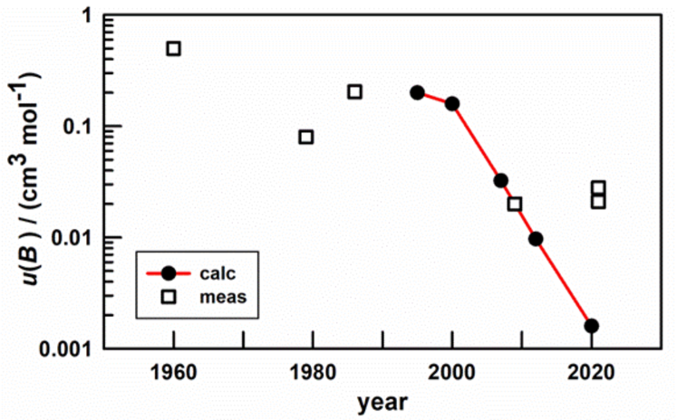
Figure 1: The standard uncertainty of both the measured and the calculated values of the second density virial coefficient of ⁴He decreased with time. After 2012, $u(B_{\mathrm{calc}})<u(B_{\mathrm{meas}})$. Both $B_{\mathrm{calc}}$ and $B_{\mathrm{meas}}$ are evaluated near 24.5561 K, which is the defined temperature of the triple point of neon. Calculated values (circles): Aziz et al. (1995) [3]; Hurly and Moldover (2000) [4]; Hurly and Mehl (2007) [5]; Cencek et al. (2012) [6]; Czachorowski et al. (2020). [7] Measured values (squares): White et al. (1960) [8]; Berry (1979) [9]; Kemp et al. (1986) [10]; Gaiser and Fellmuth (2009) [11]; Gaiser and Fellmuth (2021) [12]; Madonna Ripa et al. (2021) [13].

The paradigm reversal (replacing measured thermophysical properties of helium with calculated thermophysical properties) applies to zero-density values of the viscosity $\eta(T)$, thermal conductivity $\lambda(T)$, ³He-⁴He mutual diffusion coefficient as well as to the density and acoustic virial coefficients, relative dielectric permittivity (dielectric constant) $\varepsilon_{\mathrm{r}}(p,T)$, relative magnetic permittivity $\mu_{\mathrm{r}}(p,T)$, and refractive index $n(p,T)=\sqrt{\varepsilon_{\mathrm{r}}\mu_{\mathrm{r}}}$. For many of these properties, the values calculated for helium are standards that are used to calibrate apparatus that measures the same properties for other gases.

The paradigm reversals for $\varepsilon_{\mathrm{r}}(p,T)$ and $n(p,T)$ have been combined with technical advances in the measurement of $\varepsilon_{\mathrm{r}}(p,T)$ and $n(p,T)$ to develop novel pressure standards. One standard operating at optical frequencies and low pressures (100 Pa $\leq p\leq$ 100 kPa) is more accurate than manometers based on liquid columns. (See Section II.3.1 and Ref. 14). Other standards operating at microwave frequencies and higher pressures (100 kPa $\leq p\leq$ 7 MPa) have enabled exacting tests of mechanical pressure generators based on the dimensions of a rotating piston in a cylinder. (See Section  II.3.2 and Refs. 15, 16). At still higher pressures (up to 50 MPa), the values of helium’s density calculated from the virial equation of state (VEOS) have been used to calibrate magnetic suspension densimeters. A more accurate high-pressure scale may result. In Section II.5, we will comment on ab initio calculations of transport properties and their contribution to improved flow metrology.

During the past 25 years, the accurate calculations of the thermophysical properties of the noble gases have strongly interacted with gas-based measurements of the thermodynamic temperature $T$. To put this in context, we compare in Fig. 2 the evolution of “practical” temperature metrology with “thermodynamic” temperature metrology. [17]

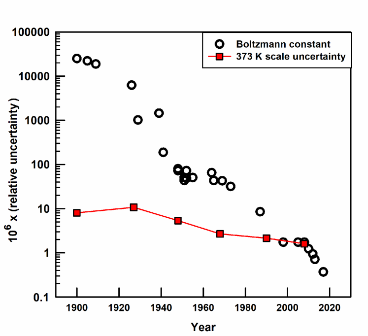
Figure 2: Comparison over time of the standard uncertainty of the Boltzmann constant to the reproducibility of the “practical” temperature scale. Circles represent the relative uncertainty of measurements of the Boltzmann constant, mostly from evaluations by groups such as CODATA. Squares represent the relative uncertainty of internationally accepted practical temperature scales in the vicinity of the normal boiling point of water. Adapted from Ref. 17.

In Fig. 2, the squares represent estimates of the relative uncertainties $u_{\mathrm{r}}(T_{\mathrm{scale}})$ of the “practical” temperature scales disseminated by National Metrology Institutes (NMIs). We plot the values of $u_{\mathrm{r}}(T_{\mathrm{scale}})$ near the boiling point of water at intervals of roughly 20 years. Most of the points are at years when the NMIs agreed to disseminate a new practical scale that was either a better approximation of thermodynamic temperatures and/or an extension of the practical scale to higher and lower temperatures. The most recent scale is the “International Temperature Scale of 1990” (ITS-90) and temperatures measured using ITS-90 are denoted $T_{90}$. The data underlying ITS-90 are constant-volume gas thermometry (CVGT) and spectral radiation thermometry linked to CVGT. [18] The pre-1990 CVGT was based on the ideal-gas equation of state, as corrected by virial coefficients either taken from the experimental literature or measured during the CVGT. Post-1990 thermometry, together with ab initio calculations of virial coefficients, revealed that the authors of ITS-90 underestimated ITS-90’s uncertainties and were unaware of its biases. (See Fig. 3 and the discussion at the end of Sec. II.2.1).

In Fig. 2, the circles represent the relative uncertainty of determinations of the Boltzmann constant $u_{\mathrm{r}}(k_{\mathrm{B}})$. To determine $k_{\mathrm{B}}$, one measures the mean energy $k_{\mathrm{B}}T$ per degree-of-freedom of a system in thermal equilibrium at the thermodynamic temperature $T$. During the interval 1960 to 2019, the thermodynamic temperature of the triple point of water was defined as $T_{\mathrm{TPW}}\equiv 273.16$ K, exactly. Thus, measurements of $k_{\mathrm{B}}T$ that were conducted near $T_{\mathrm{TPW}}$ had a negligible uncertainty from $T$ and $u_{\mathrm{r}}(k_{\mathrm{B}}T)$ was an excellent proxy for $u_{\mathrm{r}}(T)$, the uncertainty of measurements of $T$ under the most favorable conditions.

As displayed in Fig. 2, $u_{\mathrm{r}}(T_{\mathrm{scale}})$ decreased from $\sim 10$ ppm to $\sim 2$ ppm (1 ppm $\equiv$ 1 part in $10^{6}$) during the 20th century. Also during the 20th century, the relative uncertainty $u_{\mathrm{r}}(k_{\mathrm{B}})$ decreased from $\sim 200,000$ ppm to $\sim 2$ ppm. Thus, $u_{\mathrm{r}}(k_{\mathrm{B}})\gg u_{\mathrm{r}}(T_{\mathrm{scale}})$ for most of the 20th century, even though $k_{\mathrm{B}}$ was a “fundamental” constant and, therefore, a worthy challenge for metrology. The 100-fold decrease of $u_{\mathrm{r}}(k_{\mathrm{B}})$ from $\sim 40$ ppm in 1973 to $\sim 0.4$ ppm in 2017 was mostly achieved by refining the AGT measurements of $k_{\mathrm{B}}$. [19, 20]

In 1995, Aziz et al. [3] argued that the values of the thermal conductivity $\lambda(T)$, viscosity $\eta(T)$, and second density virial coefficient $B(T)$ of helium, as calculated using ab initio input, were more accurate than the best available measurements of these quantities. Subsequently, helium-based AGT measurements of $k_{\mathrm{B}}$ relied on the ab initio values of $\lambda(T)$ to account for the thermoacoustic boundary layer. Just before the Boltzmann constant was defined in 2019, the lowest uncertainty measurement of $k_{\mathrm{B}}$ used either the ab initio value of thermal conductivity of helium $\lambda_{\mathrm{He}}(273.16~{}\mathrm{K})$ or the value of $\lambda_{\mathrm{Ar}}(273.16~{}\mathrm{K})$ that was deduced from ratio measurements using $\lambda_{\mathrm{He}}(273.16~{}\mathrm{K})$ as a standard. [21, 22]

In 2019, the unit of temperature, the kelvin, was redefined by assigning the fixed numerical value $1.380649\times 10^{-23}$ to the Boltzmann constant, $k_{\mathrm{B}}$, when $k_{\mathrm{B}}$ is expressed in the unit J K^-1. Thus, the Boltzmann constant can no longer be measured. However, the temperature of the triple point of water now has an uncertainty of a few parts in $10^{7}$, although the best current value is still 273.16 K. [16]

As discussed in the next section, the techniques for measuring thermodynamic temperatures are evolving rapidly. They are becoming more and more accurate and easier to implement. We anticipate NMIs will disseminate thermodynamic temperatures instead of ITS-90 at temperatures below 25 K. This would not be possible without the accurate ab initio values of the thermophysical properties of helium.

II.2 Gas thermometry

II.2.1 Acoustic gas thermometry

During the past two decades, acoustic gas thermometry (AGT) has emerged as the most accurate primary thermometry technique over the temperature range $7$ K to $552$ K, achieving uncertainties as low as $10^{-6}T$. AGT experiments were instrumental in measuring the Boltzmann constant for the redefinition of the kelvin, [23] and have revealed small, systematic errors in the ITS-90. [18, 16] This section is necessarily brief; for an in-depth review of AGT, the reader is referred to Ref. 24.

The underlying principle of AGT is the relationship between thermodynamic temperature, $T$, and the speed of sound, $w$, in a monatomic gas:

$$w^{2}=\frac{\gamma_{0}k_{\mathrm{B}}T}{m}\left[1+\frac{\beta_{\mathrm{a}}}{RT}p+\frac{\gamma_{\mathrm{a}}}{RT}p^{2}+\ldots\right],$$ (1)

where $k_{\mathrm{B}}$ is the Boltzmann constant, $R=k_{\mathrm{B}}N_{\mathrm{A}}$ is the gas constant, $m$ is the average molecular mass of the gas, $\gamma_{0}$ is the limiting low-pressure value of $c_{p}/c_{v}$ where $c_{p}$ and $c_{v}$ are the isobaric and isochoric heat capacities, respectively, (this ratio is exactly $5/3$ for a monatomic gas), $p$ is the gas pressure, and $\beta_{\mathrm{a}}$ and $\gamma_{\mathrm{a}}$ are the temperature-dependent acoustic virial coefficients. Helium-4 or argon gas is typically used, as these are considerably less expensive than other noble gases and available in ultra-pure forms, although xenon has also been used. [26]

Most modern realizations of primary AGT determine the speed of sound from the resonance frequencies of the acoustic normal modes in a cavity resonator of fixed and stable dimensions. Resonators have been manufactured from copper, aluminium, and stainless steel, with internal volumes between 0.5 liters and 3 liters. Cavity shapes have either been spherical, quasi-spherical (with smooth, deliberate deviations from sphericity), or cylindrical. The use of diamond turning to produce quasi-spherical resonators (QSRs) with extremely accurate forms ($\sim 1~{}\mu\mathrm{m}$) and smooth surfaces (average surface roughness on the order of $\approx 3$ nm) has significantly improved performance. [27] In spherical geometries, the best results are obtained from the radially symmetric acoustic modes, since these possess high quality factors and are relatively insensitive to imperfections in the cavity shape. In cylindrical geometries, the longitudinal plane-wave modes are typically favored.

Two distinct methods of primary AGT exist: absolute and relative. In the absolute method, $T$ is determined from the limiting low-pressure ($p=0$) form of Eq. (1). The terms $\gamma_{0}$ and $k_{\mathrm{B}}$ are known exactly; $m$ must be determined by an auxiliary experiment; and $w$ is calculated from the radial acoustic mode frequencies, $f_{\mathrm{a}}$, of the QSR:

$$w=\frac{f_{\mathrm{a}}-\Delta f_{\mathrm{a}}}{z_{\mathrm{a}}}(6\pi^{2}V)^{1/3},$$ (2)

where $z_{\mathrm{a}}$ are the acoustic eigenvalues, $\Delta f_{\mathrm{a}}$ is the sum of the acoustic corrections, and $V$ is the cavity volume. If the longitudinal mode frequencies of a cylindrical cavity are used, the term proportional to $V^{1/3}$ is replaced with a multiple of the cylinder length.

Improvements in QSR volume measurements are perhaps the most significant innovation in AGT in the last two decades, and were driven by efforts to redetermine the Boltzmann constant for the redefinition of the kelvin. Modern AGT systems measure the frequency $f_{\mathrm{m}}$ of microwave resonances in the cavity, which are related to the volume through the equation

$$\frac{c}{n}=\frac{f_{\mathrm{m}}-\Delta f_{\mathrm{m}}}{z_{\mathrm{m}}}(6\pi^{2}V)^{1/3},$$ (3)

where $c$ is the speed of light in vacuum, $n$ in the refractive index of the gas in the cavity, $\Delta f_{\mathrm{m}}$ is the sum of the electromagnetic corrections, and $z_{m}$ are the microwave eigenvalues. The microwave modes do not occur in isolation, being at least 3-fold degenerate in perfectly spherical cavities. The smooth deformations of the QSR shape lift these degeneracies, enabling accurate measurement of the individual mode frequencies. A key theoretical result is that (to first order) the mean frequency of these mode groups is unaffected by volume-preserving shape deformations. [28]

In diamond-turned QSRs, the relative uncertainty in $V$ from the microwave method can be less than $1\times 10^{-6}$. [29] This was made possible by improvements in theory, [30] resonator shape accuracy, and studies of small perturbations due to probes. [29] Recently, it has been demonstrated that comparable uncertainties can be achieved with low-cost microwave equipment. [31, 32] Accurate microwave dimensional measurements have also been performed in cylindrical acoustic resonators. [33]

Relative primary AGT measures thermodynamic temperature ratios:

$$\frac{T}{T_{\mathrm{ref}}}=\frac{w^{2}}{w^{2}_{\mathrm{ref}}},$$ (4)

where $w_{\mathrm{ref}}$ is the measured speed of sound at a known reference temperature $T_{\mathrm{ref}}$. Most AGT determinations of ($T–T_{90}$) use the relative method. The main advantages are that the molecular mass term, $m$, cancels in the ratio, and that only the relative volume $V/V_{\mathrm{ref}}$ need be measured. Also, many small perturbations to the acoustic and microwave frequencies (e.g., due to shape deformations) either fully or partially cancel in the ratio. As a result, excellent results can be obtained using resonators with modest form accuracies that would be unsuited to absolute AGT. The disadvantages are that relative AGT propagates underlying errors and uncertainty in $T_{\mathrm{ref}}$, and can require the apparatus to operate over a wide temperature range when no suitable reference points are nearby.

In both absolute and relative primary AGT, maintaining gas purity is of critical importance. Impurities will shift the average molecular mass of the gas, and hence the speed of sound, by an amount that depends on the mass contrast between the bulk gas and impurity. For example, the speed of sound in helium is approximately 16 times more sensitive to water vapor than in argon. Impurities can either be present in the gas source or arise from outgassing or leaks in the apparatus itself.

Relative AGT requires only that $m$ remain unchanged between the measurements at $T$ and $T_{\mathrm{ref}}$. Temperature dependence in $m$ can arise through several mechanisms: impurities such as water, hydrocarbons, or heavy noble gases can be condensed out at low temperatures; higher temperatures ($>500$ K) cause significant outgassing from the walls of steel resonators. [34] Gas purity is vastly improved by maintaining a flow of gas (typically $<50~{}\mu\mathrm{mol}$/s) through the resonator and supply manifold.

Absolute AGT has more stringent requirements on gas purity than relative AGT. To determine an accurate value for $m$, both the isotopic abundance of the gas and any residual impurities must be quantified. Reactive impurities, including water, can be removed from the source gas using gas purifiers, and noble gas impurities can be removed from helium using a cold trap. [21] The isotopic ratios ³⁶Ar/⁴⁰Ar and ³⁸Ar/⁴⁰Ar in argon, and ³He/⁴He in helium, have been determined by mass spectrometry, and vary significantly from source to source. [35] Alternatively, isotopically pure ⁴⁰Ar gas can be used, although this is only available in small quantities and at great expense. [36]

The low uncertainty of the AGT technique arises from the excellent agreement between acoustic theory and experiment. The simplicity of Eq. (2) hides a number of temperature-, pressure-, and mode-dependent corrections that constitute the term $\Delta f_{\mathrm{a}}$. The largest of these are the thermoacoustic boundary layer corrections, which arise from an irreversible heat exchange between the oscillating gas and resonator walls. [36, 37] This effect both lowers the frequency of the acoustic resonances and broadens them; a valuable cross-check of experiment and theory can be made by comparing the predicted and measured resonance widths. The radial-mode boundary layer correction in QSRs is approximately proportional to the square root of the gas thermal conductivity – in cylinders, the gas viscosity also features in the correction. [38] For most temperature ranges, the uncertainty in these parameters can be considered negligibly small for both helium and argon due to improved ab initio calculations (see section II.5).

AGT measurements are typically conducted on isotherms in a pressure range between $25$ kPa and $500$ kPa, with the optimum pressure range depending on several factors such as the type of gas, temperature, and particular details of the apparatus. [39] At low pressures, the accuracy in determining $f_{\mathrm{a}}$ is compromised by weak acoustic signals, interference from neighboring modes due to resonance broadening, and the need to account for details of the interaction of the gas with the resonator’s walls. [40] At high pressures, higher-order virial terms are required to account for molecular interactions, and the elastic recoil of the resonator walls becomes increasingly significant. The shell recoil effect, which shifts $f_{\mathrm{a}}$ in proportion to gas density, [41] is difficult to predict in real resonators [42, 43] because of the complex mechanical properties of the joint(s) formed when the cavity resonator is assembled.

For this and other reasons, it is not common practice to use Eq. (1) to determine $T$ from $w$; instead, the measured data are fitted to low-order polynomials that account for the virial coefficients and perturbations that are proportional to pressure. Isotherm measurements have the advantage of data redundancy and reduced uncertainty, but are very slow to execute, with each pressure point taking several hours. Single-state AGT, [44] which utilizes low-uncertainty ab initio calculations of $\beta_{\mathrm{a}}$ and $\gamma_{\mathrm{a}}$ in helium, offers a much faster means of primary thermometry.

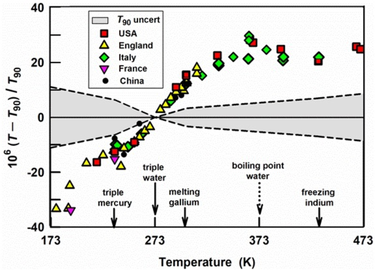
Figure 3: Post-1990 acoustic measurements of $T-T_{90}$. The shaded area encloses 1990 estimates of the fractional uncertainties of ITS-90. The acoustic measurements indicate that ITS-90 has an error of $\sim 25\times 10^{-6}T$ near water’s boiling point and $\sim-35\times 10^{-6}T$ near 173 K. The solid arrows indicate some ITS-90 fixed points. (The boiling point of water is not a fixed point on ITS-90.) Data sources: USA: Refs. 45, 34, 26; England: Refs. 46, 47; Italy: Ref. 48; France: Ref. 49; China: Ref. 50.

Figure 3 compares AGT measurements from 5 countries with ITS-90. The AGT data indicate that ITS-90 has an error of $\sim 25\times 10^{-6}T$ near water’s boiling point and $\sim-35\times 10^{-6}T$ near 173 K. Near $T_{\mathrm{TPW}}$, the derivative $\mathrm{d}T_{90}/\mathrm{d}T\approx 1+1.0\times 10^{-4}$. This implies that heat capacity measurements made using ITS-90 will generate values of the heat capacity that are 0.010% larger than the true heat capacity. However, we are not aware of heat capacity measurement uncertainties as low as 0.01%.

Prior to the AGT publications shown in Fig. 3, Astrov et al. corrected an estimate used in their CVGT. They had used measurements of the linear thermal expansion of a metal sample to estimate the thermal expansion of the volume of their CVGT “bulb”. [51] Using additional expansion measurements, Astrov et al. corrected their $T-T_{90}$ results. They now agree, within combined uncertainties, with the AGT data. (Because AGT uses microwave resonances to measure the cavity’s volume in situ, it is not subject to errors from auxiliary measurements of thermal expansion.)

II.2.2 Dielectric constant gas thermometry

DCGT, developed in the seventies in the U.K. [52, 53] and later improved by PTB, [54, 55] is now a well-established method of primary thermometry. The basic idea of DCGT is to replace the density in the equation of state of a gas by the relative permittivity (dielectric constant) $\varepsilon_{\mathrm{r}}$ and to measure it by the relative capacitance changes at constant temperature:

$$\frac{\Delta C_{\mathrm{c}}}{C_{\mathrm{c}}}\equiv\frac{C_{\mathrm{c}}(p)-C_{\mathrm{c}}(0)}{C_{\mathrm{c}}(0)}=\varepsilon_{\mathrm{r}}-1+\varepsilon_{\mathrm{r}}\kappa_{\mathrm{eff}}p.$$ (5)

In Eq. (5), $C_{\mathrm{c}}(p)$ is the capacitance of the capacitor at pressure $p$, and $C_{\mathrm{c}}(0)$ that at $p=0$ Pa and $\kappa_{\mathrm{eff}}$ is the effective isothermal compressibility which accounts for the dimensional change of the capacitor due to the gas pressure. In the low-pressure (ideal gas) limit, the working equation can be simply derived by combining the classical ideal-gas law and the Clausius–Mossotti equation:

$$p=\frac{RT}{A_{\varepsilon}}\frac{\varepsilon_{\mathrm{r}}-1}{\varepsilon_{\mathrm{r}}+2},$$ (6)

with the molar polarizability $A_{\varepsilon}$. For a real gas in a general formulation including electric fields, both input equations are power series:

$$\frac{p}{\rho RT}=1+B(T)\rho+C(T)\rho^{2}+D(T)\rho^{3}+\ldots,$$ (7)

where $B(T)$, $C(T)$, and $D(T)$ are the second, third, and fourth density virial coefficient, respectively, $\rho$ is the molar density, and

$$\frac{\varepsilon_{\mathrm{r}}-1}{\varepsilon_{\mathrm{r}}+2} = A_{\varepsilon}\rho\left(1+b\rho+c\rho^{2}+d\rho^{3}+\ldots\right)$$ (8)

$$= \rho\left(A_{\varepsilon}+B_{\varepsilon}\rho+C_{\varepsilon}\rho^{2}+D_{\varepsilon}\rho^{3}+\ldots\right).$$ (9)

In the literature, the quantities $b$, $c$, $d$ and $B_{\varepsilon}$, $C_{\varepsilon}$, $D_{\varepsilon}$ are both called the second, third, and fourth dielectric virial coefficient, respectively. The form used in Eq. (8) comes from the tradition of DCGT [52, 54] of factoring out $A_{\varepsilon}$ so that $b,c$, and $d$ have the same units as $B,C$, and $D$. Conversely, ab initio calculations naturally provide the quantities $B_{\varepsilon}$, $C_{\varepsilon}$, and $D_{\varepsilon}$.

The DCGT working equation is obtained by eliminating the density using Eqs. (7) and (8) and substituting $\varepsilon_{\mathrm{r}}$ with the relative capacitance change corresponding to Eq. (5).

This leads to a power expansion in terms of $\Xi=(\Delta C_{\mathrm{c}}/C_{\mathrm{c}})/(\Delta C_{\mathrm{c}}/C_{\mathrm{c}}+3)$:

$$p=\left(\frac{A_{\varepsilon}}{RT}+\frac{\kappa_{\mathrm{eff}}}{3}\right)^{-1}\left[\Xi+\Xi^{2}\left(\frac{A_{\varepsilon}}{RT}+\frac{\kappa_{\mathrm{eff}}}{3}\right)^{-1}\left[\frac{B-b}{RT}-\frac{\kappa_{\mathrm{eff}}}{3}\left(1+\frac{B}{A_{\varepsilon}}\right)\right]+\Xi^{3}\left(\cdots\right)\right].$$ (10)

The higher-order terms contain combinations of both the dielectric and density virial coefficients and the compressibility. Equation (10) up to the fourth order can be found in Ref. 56.

DCGT works as a primary thermometer if the molar polarizability $A_{\varepsilon}$ and virial coefficients contained in Eq. (10) are known from fundamental principles or independent measurements with sufficient accuracy. The effective compressibility $\kappa_{\mathrm{eff}}$ is also required. For classical DCGT, where isotherms are measured and the data are extrapolated to zero pressure via least-squares fitting, only $A_{\varepsilon}$ and $\kappa_{\mathrm{eff}}$ are mandatory. This was the way thermodynamic temperature was determined for decades. [52, 54, 55] Consequently, in classical DCGT, ab initio data on virial coefficients serve as a consistency check or conversely DCGT is used for determination of virial coefficients to check theory. [56] Since the theoretical calculations of the virial coefficients for helium improved drastically, it is now possible to use higher-order virial coefficients from theory to reduce the number of fitting coefficients or even to use the working equation directly without fitting and to determine temperature at each pressure point via the rearranged working equation. Recently, all three approaches have been tested and compared. [57] Especially, the point-by-point evaluation is a shift of paradigm and at the moment only possible for helium, where the uncertainty of the ab initio calculations, especially of the second density virial coefficient, is small enough. Nevertheless, for other gases not only the virial coefficients but also the molar polarizabilities determined via DCGT have comparable or smaller uncertainties than ab initio calculations. [58] This is a field of potential improvement of theory already started with calculations of $A_{\varepsilon}$ for neon [59, 60] and for argon. [61]

DCGT was operated in the temperature range from 2.5 K to about 273 K using helium-3, helium-4, neon, [62] and argon. [63] All noble gases have the advantage that the molar polarizability is independent of temperature at a level of precision far beyond that of state-of-the-art experiments. [64]

Besides the use of dielectric measurements in primary thermometry, accurate determinations of polarizability and virial coefficients of noble gases and molecules using gas-filled capacitors have a much longer tradition. These setups, very similar to DCGT, use thermodynamic temperature as one of the input parameters. A complete overview of measurements cannot be given here. Already a very broad overview of existing data, partly at radio frequencies, was summarized by NBS in the 1950’s. [65] In the following decades, [66] different institutes with changing teams performed measurements until the early 1990’s. [67] In the year 2000, NIST started measurements on gases using capacitors resulting in the most accurate values for the measured molecules. [68, 69] Very recently, PTB established a setup for separate measurement of dielectric and density virial coefficients using a combination of Burnett expansion techniques and DCGT. [70] The focus of this setup is on the determination of properties of energy gases like hydrogen-methane mixtures in the context of the transition to renewable energies.

For primary thermometry, most significant recent improvements in DCGT have been achieved by independent determination of $\kappa_{\mathrm{eff}}$ using resonant ultrasound spectroscopy around $0~{}{}^{\circ}$C and an optimal choice of capacitor materials. For the Boltzmann experiment with measuring pressures of up to 7 MPa, tungsten carbide was the ideal choice, while at low temperatures beryllium copper was used together with an extrapolation method. Relative uncertainties for $\kappa_{\mathrm{eff}}$ in terms of temperature on the level of 1 ppm near $0~{}{}^{\circ}$C have been achieved. Equally important are the improvements in pressure measurement. In contrast to AGT, where pressure is a second-order effect, in DCGT $\varepsilon_{\mathrm{r}}$ is directly linked to pressure. Therefore, the relative uncertainty in pressure can be transferred to a relative uncertainty in temperature. The major steps here are discussed in section II.3.2 regarding the mechanical pressure standard developed at PTB in the framework of the Boltzmann constant determination. [71] These systems with relative uncertainties on the level of 1 ppm at pressures up to 7 MPa have been used to calibrate commercially available systems for pressures up to 0.3 MPa with relative uncertainties between 3 ppm and 4 ppm. The dominant uncertainty component in DCGT measurements is the standard deviation of the capacitance measurement. The typical relative uncertainty in terms of temperature connected to this component is on the order of 5 ppm for the low temperature range but was reduced to the 1 ppm level in the case of the Boltzmann experiment at about $0~{}{}^{\circ}$C. [72] Finally, one problem in DCGT using helium is the very small molar polarizability compared to all other gases and molecules. Therefore, special care must be taken concerning impurities and here an especially severe issue is contamination with water.

The polarizability of water at frequencies of capacitance bridges and microwave resonators (see section V.1.2) is about a factor of 160 larger than that of helium. At cryogenic temperatures, water contamination in the gas phase is naturally reduced by outfreezing but especially at room temperature the whole measuring setup as well as the gas purifying system must be highly developed. Furthermore, pollution with other noble gases must be treated carefully because they cannot be extracted by getters and filters. Ideally, a mass-spectrometer should be used for the detection of noble gases impurities to allow for an upper estimate of the uncertainty due to gas purity. In summary, with DCGT in the low temperature range from 4 K to 25 K uncertainties on the level 0.2 mK for thermodynamic temperature are achievable. At around $0~{}{}^{\circ}$C, the smallest uncertainty for DCGT was achieved during the determination of the Boltzmann constant. [72] Converted to an uncertainty for thermodynamic temperature, this would lead to about 0.5 mK.

In the intermediate range, the uncertainties are larger (at 200 K between 1 mK and 2 mK [63]). The main restriction of the present low-temperature setup is the limited pressure range at intermediate temperatures. A measurement of high-pressure isotherms in this range is planned. Together with improved ab initio calculations for the second virial coefficients of argon and neon, a point-by-point evaluation could be possible. This could result in a significant reduction in both uncertainty and measurement time.

II.2.3 Refractive index gas thermometry

Both DCGT and RIGT are versions of polarizing gas thermometry. Both rely on virial-like expansions of either the dielectric constant $\varepsilon_{\mathrm{r}}$ or of the refractive index $n$ in powers of the molar density $\rho$, that is Eq. (9) in the case of DCGT, and the Lorentz–Lorenz equation

$$\frac{n^{2}-1}{n^{2}+2}=\rho\left(A_{\varepsilon}+A_{\mu}+B_{\mathrm{R}}\rho+C_{\mathrm{R}}\rho^{2}+\ldots\right),$$ (11)

in the case of RIGT. In the limit of zero frequency, $A_{\mu}/A_{\varepsilon}\approx-1.53\times 10^{-5}$ for He, $B_{\varepsilon}=B_{\mathrm{R}}$, $C_{\varepsilon}=C_{\mathrm{R}}$, etc. [73] Except for the small magnetic-permeability term $A_{\mu}$ (which is well-known from theory for helium [74]), low-frequency measurements of $n$ and of $\varepsilon_{\mathrm{r}}$ are analyzed using the same ab initio constants. RIGT determines the thermodynamic temperature $T$ by combining measurements of the pressure $p$ with the density virial equation of state, Eq. (7), and Eq. (11). The density is eliminated from both equations, either numerically or by iteration, to obtain

$$T=\frac{p\left(A_{\varepsilon}+A_{\mu}\right)}{R}\frac{n^{2}+2}{n^{2}-1}+\ldots$$ (12)

The constants $B$, $B_{\mathrm{R}}$, $C$, $C_{\mathrm{R}}$, etc. that appear in the higher-order terms of Eq. (12) are obtained either from theory or from fitting measurements of $n^{2}(p)$ on isotherms. [DCGT determines $T$ using a version of Eq. (12) in which $\varepsilon_{\mathrm{r}}$ replaces $n^{2}$.]

Here, we focus on RIGT conducted at microwave frequencies as developed by Schmidt et al. [75] and as recently reviewed by Rourke et al. [76] These authors determined $n$ from measurements of the microwave resonance frequencies $f_{\mathrm{m}}$ of a gas-filled, metal-walled, quasi-spherical cavity. Typical frequencies ranged from 2.5 GHz to 13 GHz; for this range, the frequency dependence of $n$ in the noble gases is negligible. As discussed in Sec. II.3.1, RIGT has also been realized at optical frequencies in the context of pressure standards. [77] For helium, the corrections of $A_{\varepsilon}$ and $B_{\mathrm{R}}$ from optical frequencies to zero frequency have been calculated ab initio. [73, 78]

A working equation for measuring $n$ is:

$$n=\sqrt{\mu\varepsilon_{\mathrm{r}}}=\frac{\langle f_{\mathrm{m}}+g\rangle_{\mathrm{vacuum}}}{\langle f_{\mathrm{m}}+g\rangle_{\mathrm{pressure}}(1-\kappa_{\mathrm{eff}}p)},$$ (13)

where the brackets “$\langle\rangle$” indicate averaging over the frequencies of a nearly degenerate microwave multiplet and $g$ accounts for the penetration of the microwave fields into the cavity’s walls. Usually, $g$ is determined from measurements of the half-widths of the resonances; its contribution to uncertainties is small. The term $\kappa_{\mathrm{eff}}p$ accounts for the temperature-dependent change of the cavity’s volume in response to the gas pressure $p$. Often, the uncertainty of $\kappa_{\mathrm{eff}}$ is the largest contributor to the uncertainty of RIGT. To make this explicit, we manipulate Eqs. (12) and (13) to obtain:

$$T=\frac{3p}{R}\left(\frac{A_{\varepsilon}+A_{\mu}}{n^{2}-1}\right)\left(1-\frac{2\kappa_{\mathrm{eff}}RTn^{2}}{3(A_{\varepsilon}+A_{\mu})}\right)+\ldots,$$ (14)

where the term $2\kappa_{\mathrm{eff}}RTn^{2}/[3(A_{\varepsilon}+A_{\mu})]\approx 0.007$ for a copper-walled cavity immersed in helium near $T_{\mathrm{TPW}}$. (This estimate assumes that the cavity’s walls are homogeneous and isotropic; therefore, $\kappa_{\mathrm{eff}}=\kappa_{T}/3$ where $\kappa_{T}$ is the isothermal compressibility of copper.) Thus, a relative uncertainty $u_{\mathrm{r}}(\kappa_{\mathrm{eff}})=0.01$ contributes the relative uncertainty $u_{\mathrm{r}}(T_{\mathrm{TPW}})=70\times 10^{-6}$ to a RIGT determination of $T_{\mathrm{TPW}}$. In the approximation $n^{2}\approx 1$, this uncertainty contribution is a function of $T\times\kappa_{\mathrm{eff}}(T)$, but it is not a function of the pressures measured on an isotherm. Because $T\times\kappa_{\mathrm{eff}}(T)$ decreases with $T$, RIGT is more attractive at cryogenic temperatures than near or above $T_{\mathrm{TPW}}$.

Recently, two independent groups explored a two-gas method for measuring $\kappa_{\mathrm{eff}}$ of assembled RIGT resonators. [79, 13] Ideally, two-gas measurements would replace measurements of $\kappa_{T}$ of samples of the material comprising the resonator’s wall and also models for the cavity’s deformation under pressure. Both groups relied on new, accurately measured and/or calculated values of the density and refractivity virial coefficients of neon or argon. [73, 56] Using helium and argon, Rourke determined $\kappa_{\mathrm{eff}}$ at $T_{\mathrm{TPW}}$ with the remarkably low uncertainty $u_{\mathrm{r}}(\kappa_{\mathrm{eff}})=9.6\times 10^{-4}$. [79] Madonna Ripa et al. combined helium and neon data to reduce the uncertainty contribution from $\kappa_{\mathrm{eff}}$ to their determinations of $T$ at the triple points of O₂ ($\approx 54$ K), Ar ($\approx 84$ K), and Xe ($\approx 161$ K). [13] They reported “partial success” and suggested that a revised apparatus using both gases and operating at higher pressures ($p>500$ kPa) would obtain lower uncertainty determinations of $T$. They also noted that the two-gas method requires twice as much RIGT data, accurate pressure measurements, and dimensional stability between gas fillings

Rourke’s review of RIGT [76] noted 5 groups implementing RIGT using microwave technology. In contrast, we are aware of only one group (at PTB) implementing DCGT. [57] The relative popularity of RIGT results from the commercial availability of vector analyzers that can measure microwave frequency ratios with resolutions of $10^{-9}$. To our knowledge, using commercially available capacitance bridges, the highest attainable capacitance ratio resolution is $70\times 10^{-9}$. [80] To attain higher resolution for DCGT, PTB developed a unique bridge that measures capacitance ratios with a resolution of order $10^{-8}$ in a 1 s averaging time. To achieve this specification, the PTB bridge must operate at 1 kHz and both the standard (evacuated) capacitor and the unknown (gas-filled) capacitor must have identical construction and be located in the same thermostat. [81]

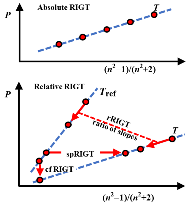
Figure 4: Measurement trajectories for RIGT in the variables pressure ($p$) and refractive index ($n$). Blue dashed lines represent isotherms. Top: Absolute RIGT takes many data points on an isotherm at the unknown temperature $T$. Bottom: Relative rRIGT takes several measurements on a reference isotherm $T_{\mathrm{ref}}$ and on an unknown isotherm $T$. Single pressure (spRIGT) uses data at one pressure. Constant frequency (cfRIGT) uses data at one value of the refractive index $n$.

Figure 4 illustrates the several strategies being explored for acquiring RIGT data. Absolute RIGT acquires many $(p,n)$ data on an isotherm and determines $T$ via Eq. (14). This method requires state-of-the-art, absolute pressure measurements; therefore, the pressure gradient between the gas-filled cavity and the manometer (normally at ambient temperature) is required. [82] Uncertainty budgets for absolute RIGT can be found in Refs. 79, 13.

Relative RIGT (rRIGT) comes in several flavors, each designed to simplify some aspect of absolute RIGT. Each flavor requires measurements on at least two isotherms: (1) a reference isotherm $T_{\mathrm{ref}}$ for which the thermodynamic temperature is already well known, and (2) an unknown isotherm for which $T$ will be determined. As suggested in the lower panel of Fig. 4, one flavor of rRIGT determines $T/T_{\mathrm{ref}}$ by determining the low-pressure limit of the ratio of slopes [75]

$$\frac{T}{T_{\mathrm{ref}}}=\lim_{p\to 0}\left(\frac{n^{2}_{T}-1}{n^{2}_{T_{\mathrm{ref}}}-1}\right).$$ (15)

If $T_{\mathrm{ref}}$ and $T$ are low temperatures, where the pressure deformation of the cavity $\kappa_{\mathrm{eff}}p$ is small, this strategy circumvents the problem of accurately determining $\kappa_{\mathrm{eff}}$.

Single-pressure RIGT (spRIGT) measures $(p,n,T)$ and $(p,n,T_{\mathrm{ref}})$ and determines $T$ from $T/T_{\mathrm{ref}}\approx(n^{2}_{T}-1)/(n^{2}_{T_{\mathrm{ref}}}-1)$. This strategy entirely avoids accurate pressure measurements; instead, the pressure in the cavity is required to be identical when $n$ is measured at $T$ and $T_{\mathrm{ref}}$ and the pressure (actually, the gas’ density) must be sufficiently low that an approximate pressure is adequate for making the virial corrections. This strategy was used by Gao et al. for RIGT between the triple point of neon ($T_{\mathrm{ref}}\approx 24.5$ K) and 5 K. [83] After establishing $T_{\mathrm{ref}}$ by acoustic thermometry, they claimed the uncertainties of this implementation of RIGT were smaller than the uncertainties of ITS-90. [84]

When constant-frequency RIGT (cfRIGT) is implemented, the pressure in the cavity is changed to keep the refractive index constant as the temperature is changed from $T_{\mathrm{ref}}$ to $T$. In this case, $T/T_{\mathrm{ref}}\approx p(T,n)/p(T_{\mathrm{ref}},n)$. [85] This scheme minimizes the frequency-dependent effects of the coaxial cables on the microwave determination of $T/T_{\mathrm{ref}}$.

To economically search for measurement or modeling errors, one can obtain 3 redundant values of $T/T_{\mathrm{ref}}$ by measuring microwave frequencies at 4 judiciously chosen values of $(p,n)$. Two measurements are made on the isotherm $T_{\mathrm{ref}}$ at the values $(p_{1},n_{1})$ and $(p_{2},n_{2})$. Two other measurements are on the isotherm $T$ at $(p_{2},n_{3})$ and $(p_{3},n_{1})$. spRIGT connects the points $(p_{2},n_{2})$ and $(p_{2},n_{3})$. cfRIGT connects the points $(p_{1},n_{1})$ and $(p_{3},n_{1})$. All 4 points are used to approximately implement rRIGT via Eq. (15).

Compared with other forms of gas thermometry, relative RIGT has significant advantages at low temperatures. We have already emphasized the availability of microwave network analyzers and the possibility of avoiding state-of-the art pressure measurements. By measuring several microwave resonance frequencies at each state, certain imperfections of the measurements and modeling can be detected. Comparisons of the frequencies of TE and TM microwave modes might detect the presence of dielectric films such as oxides, oil deposits, or adsorbed water on the cavity’s walls. [86] Because relative RIGT relies on microwave frequency ratios, the precise shape of the cavity is unimportant. Cavity shapes other than quasispheres may be advantageous in particular applications.

RIGT is simpler and more rugged than relative acoustic gas thermometry (rAGT) because RIGT requires neither delicate acoustic transducers nor acoustic ducts. However, RIGT is unlikely to replace rAGT at ambient and higher temperatures because RIGT is more sensitive to the cavity’s dimensions than rAGT by the factor $1/(\varepsilon_{\mathrm{r}}-1)$ which typically ranges from 200 to 20000. Furthermore, microwave RIGT is especially sensitive to polar impurities. Adding 1 ppm (mole fraction) of water vapor to dilute argon gas at 293 K will increase the gas’ dielectric constant by 18 ppm and increase the square of the gas’ speed-of-sound by 0.12 ppm. If the water vapor were undetected, these changes would reduce the argon’s apparent RIGT temperature by 18 ppm and argon’s apparent rAGT temperature by $-0.12$ ppm. For helium, the corresponding temperature reductions are 145 ppm and 4 ppm.

II.2.4 Constant volume gas thermometry

The website of the International Bureau of Weights and Measures includes a document (“Mise en pratique $\ldots$”) that indicates how the SI base unit, the kelvin, may be realized in practice using 4 different versions of gas thermometry. [87] Surprisingly, this document omits CVGT, the version of gas thermometry that was the primary basis of ITS-90. In this section, we briefly describe the operation of a particular realization of CVGT and the inconsistent results it generated. This may explain why CVGT was omitted from the Mise en pratique. We mention the post-1990 theoretical and experimental developments that suggest an updated realization of CVGT might generate very accurate realizations of the kelvin.

CVGT at NBS/NIST began in 1928 and concluded in 1990. We denote the most-recent realization of NBS/NIST’s relative CVGT by “CV_NIST90”. The heart of CV_NIST90 was a metal-walled, cylindrical cavity (“gas bulb”; $V\sim 407$ cm³) attached to a “dead space” comprised of a capillary leading from the bulb to a constant-volume valve at ambient temperature. The valve separated the gas bulb from a pressure-measurement system. A typical temperature measurement using CV_NIST90 began by admitting $N_{\mathrm{r}}\sim 0.0023$ mol of helium into the gas bulb at a measured reference pressure ($p_{\mathrm{r}}\sim 13$ kPa) and a measured reference temperature ($T_{\mathrm{r}}\sim T_{\mathrm{TPW}}$). [88, 89] Then, the valve was closed to seal the helium in the gas bulb and dead space. The bulb was moved into a furnace that was maintained at the unknown temperature $T$ to be determined by CVGT. After the gas bulb equilibrated, the valve was opened to measure the pressure $p$ again. The temperature ratio $T/T_{\mathrm{r}}$ was determined by applying the virial equation at each temperature:

$$\frac{T}{T_{\mathrm{r}}}=\frac{pV_{T}}{N_{T}R\left(1+(BN/V)_{T}+\ldots\right)}\frac{N_{\mathrm{r}}R(1+(BN/V)_{\mathrm{r}}+\ldots)}{p_{\mathrm{r}}V_{\mathrm{r}}}$$ (16)

Thus, $T/T_{\mathrm{r}}$ is determined, in leading order, by the three ratios: $p/p_{\mathrm{r}}$, $V_{T}/V_{\mathrm{r}}$, and $N_{\mathrm{r}}/N_{T}$. For CV_NIST90, $N_{\mathrm{r}}/N_{T}\neq 1$ because a tiny quantity of helium flows from the bulb into the capillary when the bulb is moved into the furnace. This quantity was calculated using the measured temperature distribution along the capillary. For CV_NIST90, $V_{T}/V_{\mathrm{r}}$ was calculated using auxiliary measurements of the linear thermal expansion of samples of the platinum-rhodium alloy comprising the gas bulb. These samples had been cut out of the gas bulb after completing all the CVGT measurements.

The simplicity of Eq. (16) hides the many complications of CVGT. We mention three examples. (1) During pressure measurements, helium outside the gas bulb was maintained at the same pressure as the helium inside the gas bulb. (2) Thermo-molecular and hydrostatic pressure gradients in the capillary were taken into account. (3) At high temperatures, creep in the gas bulb’s volume was detected by time-dependent pressure changes; the pressure was extrapolated back in time to its value when the bulb was placed in the furnace.

We denote the second most recent realization of NBS/NIST’s relative CVGT by “CV_NBS76”. [90] Both CV_NIST90 and CV_NBS76 shared apparatus and many procedures. However, Ref. 88 lists 11 significant changes. Here, we mention only one. CV_NIST90’s two cylindrical, gas bulbs had been fabricated entirely from sheets of (80 wt% Pt + 20 wt% Rh) alloy. The sides and bottom of CV_NBS76’s gas bulb were fabricated from the same alloy; however, the top of the bulb was inadvertently fabricated from (88 wt% Pt + 12 wt% Rh) alloy. Perhaps the slight differences in thermal expansions of these alloys led to an anomalous thermal expansion of the volume of CV_NBS76’s gas bulb.

Unfortunately, the results from CV_NIST90 and CV_NBS76 were inconsistent, within claimed uncertainties, in the range of temperature overlap (505 K $\leq T\leq$ 730 K). An approximate expression for the differences is: $T_{\mathrm{NIST90}}-T_{\mathrm{NBS76}}\approx 0.090\times(T/\mathrm{K}-400)$ mK. This inconsistency was not explained by the authors of CV_NIST90 nor by the authors of CV_NBS76. Furthermore, the authors did not assert the more recent CV_NIST90 results were more accurate than the earlier CV_NBS76 results. The working group that developed ITS-90 had no other data, from NIST or elsewhere, that were suitable for resolving the inconsistency. Therefore, the working group required ITS-90 to be the average of $T_{\mathrm{NIST90}}$ and $T_{\mathrm{NBS76}}$ in the overlap range. [91]

In the range 2.5 K to 308 K, ITS-90 relied, in part, on another realization of CVGT that had a troubled history. Astrov et al. deduced the thermal expansion of their copper gas bulb’s volume from measurements of the linear thermal expansion of copper samples taken from the block used to manufacture their bulb. [92] However, the thermal expansion data were inconsistent with other data for copper. Astrov’s group repeated the thermal expansion measurements using another (better) dilatometer. The more recent expansion data, published in 1995, changed the values of $T$ by more than $50\times 10^{-6}T$ in the range 130 K $<T<$ 180 K, where the uncertainties had been estimated as $\leq 26\times 10^{-6}T$. [51]

Recently, a working group of the Consultative Committee for Thermometry reviewed primary thermometry below 335 K. [16] Astrov’s revised CVGT values are close to the current consensus, which is primarily based on AGT and DCGT. The working group retained three other low-temperature realizations of CVGT. Post-1990 AGT measurements of $T-T_{90}$ near 470 K and 552 K indicate that CV_NIST90 is indeed more accurate than CV_NBS76. [45] Despite the fact that CVGT was the primary basis for the ITS-90, the Mise en pratique does not include CVGT. We speculate that no temperature metrology group is pursuing CVGT because: (1) CVGT is complex, (2) Astrov et al.’s thermal expansion problem, (3) unexplained problems with NBS/NIST’s CVGT, and (4) rapid advances in other versions of gas thermometry.

We now ask: is CVGT a viable method of primary thermometry today? The gas bulb of a modern CVGT would incorporate feedthroughs to enable measuring microwave resonance frequencies of the bulb’s cavity. The resonance frequencies would determine the bulb’s volumetric thermal expansion, thereby avoiding auxiliary measurements of linear thermal expansion and also avoiding the assumption of isotropic expansion. If the bulb incorporated a valve and a differential-pressure-sensing diaphragm, the dead-space corrections would vanish. (The diaphragm’s motion could be detected using optical interferometry.) Today, the ab initio values of $B(T)$ would reduce the uncertainty component from $B(T)$ to near zero. A contemporary CVGT could operate at $\sim 5\times$ higher helium densities than published experiments without generating significant uncertainties from either the virial coefficients or from pressure-ratio measurements. The higher density, together with simultaneous pressure and microwave measurements, might enable separation of the bulb’s creep from contamination by outgassing. Most outgassing contaminants affect helium’s dielectric constant, refractivity, and speed of sound much more than they affect helium’s pressure, an advantage of CVGT. However, CVGT inherently uses fixed aliquots of gas. Therefore, CVGT cannot benefit from flowing gas techniques that have been used, for example, in high-temperature AGT. [45] In summary, contemporary CVGT could be competitive with other forms of primary gas thermometry, with a possible exception at the highest temperatures, where flowing gas might be required to maintain gas purity.

II.3 Pressure metrology

Traditionally, standards based on the realization of the mechanical definition of pressure, the normal force applied per unit area onto the surface of an artifact, include pressure balances and liquid column manometers. The combined overall pressure working range of these instruments extends over seven orders of magnitude, roughly between 10 Pa and 100 MPa. Liquid column manometers achieve their best performance, with relative standard uncertainty as low as 2.5 ppm, near their upper working limit at a few hundred kPa. [93] With a few notable exceptions, the typical relative standard uncertainty of pressure balances spans between nearly $1\times 10^{-3}$ at 10 Pa, the lowest end of their utilization range, down to 2 to 3 ppm in the range between 100 kPa and 3 MPa. [93, 94] One such exception is the remarkable achievement of a relative standard uncertainty as low as 0.9 ppm for the determination of helium pressures up to 7 MPa, [71] though this achievement required the extensive dimensional characterization, and the cross-float comparison, of the effective areas of six piston–cylinder sets manufactured to extraordinarily tight specifications, with a research effort lasting several years. In spite of this outstanding result, the accurate characterization of pressure balances is challenging, due to the complexity of the dimensional characterization of the cross-sectional area of piston-cylinder assemblies, which includes finite-element modeling of their deformation under pressure. [95, 96] International comparisons periodically provide realistic estimates of the average uncertainty of realization of primary standards among NMIs. In 1999, a comparison of primary mechanical pressure standards in the range 0.62 MPa $<p<$ 6.8 MPa, involving five NMIs leading in pressure metrology exchanging a selected piston-cylinder set, was completed. [97] The resulting differences $\Delta A_{\mathrm{eff}}\equiv 10^{6}(A_{\mathrm{eff}}/\langle A_{\mathrm{eff}}\rangle-1)$ of the effective area $A_{\mathrm{eff}}$ of the piston from the reference value $\langle A_{\mathrm{eff}}\rangle$ spanned beyond their combined uncertainties with such significant spread to show that the pressure standards realized by different NMIs were mutually inconsistent.

These inconsistencies strengthened the motivation for the development of standards realizing a thermodynamic definition of pressure by the experimental determination of a physical property of a gas having a calculable thermodynamic dependence on density, combined with accurate thermometry. This possibility was initially proposed in 1998 by Moldover, [98] who envisaged, already at that time, the potential of first-principles calculation to accurately predict the thermodynamics and electromagnetic properties of helium and the maturity of experiments determining the dielectric constant using calculable capacitors. The metrological performance of thermodynamic pressure standards has continuously improved over the last two decades to become increasingly competitive in terms of accuracy, providing important alternatives which may test the exactness of the mechanical standards discussed above and eventually replace some of them. Also, due to their reduced complexity and bulkiness, simplified versions of thermodynamics-based standards may be more flexibly adapted to specific technological and scientific applications of pressure metrology. The best-performing recent realizations of gas-based pressure standards include measurements of the dielectric constant using capacitors and of the refractive index at microwave and optical frequencies, respectively using resonant cavities and Fabry–Pérot refractometers. In Secs. II.3.1 and II.3.2, we separately discuss the most notable of these developments depending on the pressure range of their application.

II.3.1 Low pressure standards (100 Pa to 100 kPa)

In the low vacuum regime, several experimental methods are available which may provide alternative routes for traceability to the pascal. For the cases involving optical measurements, these methods include: (1) refractometry (interferometry), implemented in various configurations that employ single or multiple cavities or cells with fixed or variable path lengths; (2) line-absorption methods. The achievements and perspectives of all these methods were recently reviewed. [99]

At present, Fabry–Pérot refractometry with fixed length optical cavities (FLOC) has demonstrated the lowest uncertainty for the realization of pressure standards near atmospheric pressure and down to 100 Pa. In principle, the uncertainty of this method is limited by several optical and mechanical effects, most importantly by the change in the length of the cavity due to compression by the test gas, with the same sensitivity to the imperfect estimate of the compressibility $\kappa_{T}$ that affects RIGT. However, this major uncertainty contribution may be drastically reduced, though not completely eliminated, by measuring the pressure-induced length change of a second reference FLOC monolithically built on the same spacer, which is kept continuously evacuated. In 2015, a dual-cavity FLOC achieved an extremely accurate determination of the refractive index of nitrogen at $\lambda=632.9908$ nm, $T=302.9190$ K and 100.0000 kPa by reference to the pressure realized by a primary standard mercury manometer, and using refractive index measurements in helium to determine the compressibility. [100] A comparison of the pressures determined by the nitrogen refractometer with the mercury manometer below the primary calibration point at 100 kPa down to 100 Pa showed relative differences within 10 ppm. A direct comparison between laser refractometry with nitrogen and a mercury manometer was realized one year later also at NIST. [14] The comparison showed relative differences between these instruments within 10 ppm over the range between 100 Pa and 180 kPa. The laser refractometer outperforms the precision and repeatability of the liquid manometer and demonstrates a pressure transfer standard below 1 kPa that is more accurate than its current primary realization. Such remarkably low uncertainty also favorably compares to the best dimensional characterization and modeling of non-rotating piston-cylinder assemblies.[101]

In 2017, more accurate measurements in helium and nitrogen were performed between 320 kPa and 420 kPa using a triple-cell heterodyne interferometer referenced to a carefully calibrated piston gauge, showing relative differences within 5 ppm with uncertainties on the order of 10 ppm. [77] Some pressure distortion errors affecting FLOC might in principle be eliminated by refractive index measurement with a variable length optical cavity (VLOC). The realization of this technique requires extremely challenging dimensional measurements, with displacements on the order of 15 cm that must be determined with picometer uncertainty. [102] Gas modulation techniques, with the measuring cavity frequently and repeatedly switched between a filled and evacuated condition, have been recently developed [103, 104] aiming at the reduction of the effects of dimensional instabilities and other short- and long-term fluctuations that affect Fabry–Pérot refractometers. A novel realization of an optical pressure standard, based on a multi-reflection interferometry technique, has also been recently developed, demonstrating the possible realization of the pascal with a relative standard uncertainty of 10 ppm between 10 kPa and 120 kPa. [105] Optical refractometry for pressure measurement is also being pursued at other NMIs. [106, 107]

At microwave frequencies, the realization of a low-pressure standard requires a substantial enhancement in frequency resolution. Recently, it was demonstrated by Gambette et al. that by coating the internal surface of a copper cavity with a layer of niobium, and working at temperatures below 9 K where niobium becomes superconducting, pressures in the range between 500 Pa and 20 kPa can be realized very precisely. [108, 109] The overall relative standard uncertainty of this method is currently 0.04%, with the largest contribution from non-state-of-the-art thermometry, which is likely to be substantially reduced in future work.

II.3.2 Intermediate pressure standards (0.1 MPa and 7 MPa)

Differently than initially envisaged, the first realization of a thermodynamic pressure standard was not obtained by capacitance measurements, but using a microwave resonant cavity working in the GHz frequency range, i.e., by a RIGT method. A main motivation for this choice was the development of quasi-spherical microwave resonators, whose internal triaxial ellipsoidal shape slightly deviates from that of a perfect sphere. [86] This particular geometry resolved the intrinsic degeneracy of microwave modes, allowing enhanced precision in the determination of resonance frequencies.

By 2007, Schmidt et al. [75] demonstrated a pressure standard based on the measurement of the refractive index of helium to achieve overall relative pressure uncertainty $u_{\mathrm{r}}(p)$ within $9\times 10^{-6}$ between 0.8 MPa and 7  MPa. At the upper limit of the pressure range, the uncertainty was dominated by the uncertainty of the isothermal compressibility $\kappa_{T}$ of maraging steel, which was determined using resonance ultrasound spectroscopy (RUS). [110] Recently, Gaiser et al. [15] realized Moldover’s original proposal of a capacitance pressure standard using DCGT techniques that they had refined during their measurements of the Boltzmann constant. They achieved the remarkably low uncertainty $u_{\mathrm{r}}(p)=4.4\times 10^{-6}$ near 7 MPa. Recently, the same experimental data were re-analyzed to take advantage of the increased accuracy of the ab initio calculation of the second density virial coefficient $B$ of He, [7] reducing the overall uncertainty of the capacitance pressure standard to $u_{\mathrm{r}}(p)=2.2\times 10^{-6}$. [111]

At pressures below 1 MPa, the uncertainty of the realization of a pressure standard based on DCGT or RIGT with helium is limited by the resolution of relative capacitance or frequency measurements. This limit would be immediately reduced by up to one order of magnitude by using, instead of helium, a more polarizable gas like neon or argon. However, while a significant improvement of the interaction potential, and hence of the ab initio calculated $B$, has recently been achieved for neon [112] and it is well underway for Ar, [113] it is not likely that the best available calculations of the molar polarizability $A_{\varepsilon}$ of neon [60] or argon [61] can be improved sufficiently to replace experiment in the near future. However, an experimental estimate of $A_{\varepsilon}$ of both neon and argon was obtained by comparative DCGT measurements relative to helium, with relative uncertainty of 2.4 ppm, [58] and may now be used for the realization of pressure standards with other apparatus. For similar purposes, the ratio of the refractivity of several monatomic and molecular gases, namely Ne, Ar, Xe, N₂, CO₂, and N₂O, to the refractivity of helium was determined at $T=293.15$ K, $\lambda\sim 633$ nm, with standard uncertainty within $16\times 10^{-6}$, using interferometry. [114] At pressures higher than a few MPa, the imperfect determination of the deformation of the cavity under pressure would impact the overall uncertainty of a pressure standard based on RIGT or DCGT. One possibility to tackle this limit would be a two-gas scheme where the compressibility $\kappa_{T}$ of an apparatus would be first precisely determined by measurements with helium along an isotherm and then used to realize a pressure standard with a different working gas. The same strategy is also applied to increase the upper pressure range where refractometry methods like FLOC can be applied, though use of helium for the determination of distortion effects requires correcting for diffusion within the glasses used for the construction of these apparatuses. [115]

II.4 High pressures and equation of state

Up to this point, we have considered interactions between temperature and pressure standards and the rigorously calculated, low-density properties of the noble gases including the polarizability and second and third density and dielectric virial coefficients. We now compare ab initio calculations with measurements at pressures above 7 MPa and at correspondingly higher densities. The literature includes temperature-dependent values of 6 density virial coefficients of helium, [116] 7 acoustic virial coefficients of krypton, [117] and 6 density virial coefficients of argon. [118] These calculations used the best ab initio two-body and nonadditive three-body potentials that were available at the time of publication. Many-body non-additive potentials involving four or more bodies, which are needed for the exact calculation of virial coefficients from the fourth onwards, are not available and are generally neglected, resulting in an uncontrolled approximation. Here, we compare measurements of the density of helium $\rho_{\mathrm{meas}}(p,T)$ with values calculated ab initio. This comparison avoids fitting $\rho_{\mathrm{meas}}(p,T)$ to the VEOS because such fits yield highly correlated values for the separate virial coefficients, each with large uncertainties. Later in this section, we comment on comparisons using speed-of-sound data.

Measurements of gas densities with uncertainties below 0.1% are expensive and rare because they are not required for chemical and mechanical engineering. The uncertainties of most process models are dominated by imperfect models of equipment (heat exchangers, compressors, distillation columns, etc.) and/or imperfect knowledge of the composition of feedstocks and products. An example of a demanding application of gas density and composition measurements is custody transfer of natural gas as it flows through large pipelines near ambient temperature and at high pressures (e.g., 7 MPa). An international comparison among NMIs achieved a $k=2$ volumetric flow uncertainty of only 0.22%. [119] In this context, density and composition measurements with uncertainties of order 0.1% are satisfactory for converting volumetric flows into mass flows and heating values.

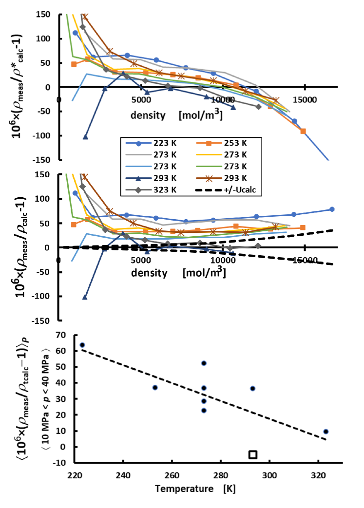
Figure 5: Top: Differences (in parts per million) on isotherms between measured densities and the densities calculated using the ab initio terms $B\rho,C\rho^{2},D\rho^{3}$, in the truncated VEOS. Middle: Same as top with additional theoretical terms: $E\rho^{4},F\rho^{5}$. All data with $\rho_{\mathrm{meas}}>4000$  mol/m³ are within 80 ppm of $\rho_{\mathrm{calc}}$. The claimed uncertainty of $\rho_{\mathrm{meas}}$ is the span of the figure: $\pm 150$ ppm. The dashed curves (- -) bound the estimated uncertainty of $\rho_{\mathrm{calc}}$ at 223 K. Bottom: Averaged deviations from $\rho_{\mathrm{calc}}$ for each isotherm in the high-pressure range 10 MPa $<p<$ 40 MPa. The dashed line fitted to the points corresponds to calibrating the temperature-dependence of the sinker’s density using the helium VEOS. The symbol $\square$ identifies an anomalous isotherm that was measured with helium of lesser purity.

In Fig. 5, the remarkable data of McLinden and Lösch-Will are used to test the ab initio VEOS of helium in the ranges 1 MPa $<p<$ 38 MPa and 223 K $<T<$ 323 K. [120] These data were acquired using a magnetic suspension densimeter. A weigh scale determined the buoyant forces on two “sinkers” immersed in the helium. The data are precise, well-documented, and traced to SI standards with a claimed, $k=2$, density uncertainty of 0.015% + 0.001 kg/m³ at the temperature extremes and at the highest density. These features attracted previous comparisons with theory. [121, 116, 122]

For the present comparison, where recently published theoretical values of the virial coefficients are used, we converted the measured temperatures from the ITS-90 to thermodynamic temperatures using Ref. 16 and we converted the measured mass densities to molar densities using the defined value of the universal gas constant and the molar mass for McLinden and Lösch-Will’s helium sample. At densities below $\sim 4000$ mol/m³, the uncertainties and the values of ($\rho_{\mathrm{meas}}/\rho_{\mathrm{calc}}-1$) diverge on isotherms as $\rho^{-1}$ and/or $p^{-1}$. (See Fig. 5.) These low-density divergences result from time-dependent drifts in the zeros of the densimeter and/or pressure transducer. Because the divergences contain more information about the apparatus than about the helium’s VEOS, we do not discuss them.

At densities above 4000 mol/m³, we compared the $\rho_{\mathrm{meas}}(p,T)$ data of McLinden and Lösch-Will [120] with the values of $\rho_{\mathrm{calc}}^{*}(p,T)$ that are implicitly defined by the truncated VEOS:

$$\frac{p}{\rho_{\mathrm{calc}}^{*}RT}=1+B_{\mathrm{calc}}\rho_{\mathrm{calc}}^{*}+C_{\mathrm{calc}}{\rho_{\mathrm{calc}}^{*}}^{2}+D_{\mathrm{calc}}{\rho_{\mathrm{calc}}^{*}}^{3}$$ (17)

The fully quantum-mechanical values of $B_{\mathrm{calc}},C_{\mathrm{calc}}$, and $D_{\mathrm{calc}}$ (the latter computed neglecting four-body interactions) were taken from Refs. 7, 123, 122, respectively. The top panel of Fig. 5 shows that the differences trend downward as the densities increase above about 4000 mol/m³. This trend, as a function of $(p,T)$, was noted in Ref. 122, together with the suggestion “there may have been a small error in the calibration for the sinkers $\ldots$” However, the trend (Fig. 5, top) plotted as a function of density suggests that $\rho_{\mathrm{meas}}$ is sensitive to some of the truncated virial coefficients. The truncation suggestion is confirmed by the middle panel of Fig. 5, which includes in $\rho_{\mathrm{calc}}(p,T)$ the two additional terms $E_{\mathrm{calc}}(T)\rho^{4}$ and $F_{\mathrm{calc}}(T)\rho^{5}$ calculated semi-classically in Ref. 116. Additional terms (e.g., $G_{\mathrm{calc}}(T)\rho^{6}$ from Ref. 116) are less than 1.3 ppm, too small to be visible in Fig. 5.

The claimed $k=2$ uncertainty of $\rho_{\mathrm{meas}}$ is 150 ppm; [120] the span of the upper panels of Fig. 5 is $\pm 150$ ppm. The dashed curves (- -) in the middle panel of Fig. 5 represent upper bounds to the uncertainty of $\rho_{\mathrm{calc}}(T,\rho)$ at 223 K. For these upper bounds, we used the $k=2$ uncertainties of the virial coefficients $U(B),U(C),\ldots$ provided by their authors. In Eq. (17) we replaced $B$ with $B+U(B)$; we replaced $C$ with $C+U(C)$, etc. The uncertainties of $\rho_{\mathrm{calc}}(T,\rho)$ are smaller at higher temperatures. We conclude $\rho_{\mathrm{calc}}$ agrees with $\rho_{\mathrm{meas}}$ well within combined uncertainties.

At densities above $\sim 4000$ mol/m³, the differences ($\rho_{\mathrm{meas}}/\rho_{\mathrm{calc}}-1$) are nearly independent of the density; however, the average densities are 34 ppm larger than their expected values $\rho_{\mathrm{calc}}$. These offsets are well within the claimed measurement uncertainties ($k=2$, $\sim 150$ ppm). However, as shown in the lower panel of Fig. 5, the offsets have both a random and a systematic dependence on the temperature. The systematic temperature-dependence can be treated as a correction to the calibration of the sinkers’ densities $\rho_{\mathrm{sinker}}(p,T)$. Such a correction does not remove the spread ($\pm 14$ ppm) among the 4 isotherms at 273 K. Possible causes of this spread are changes between runs of temperature ($\pm 3.8$ mK) and/or of impurity content (e.g., $\pm 2.3$ ppm of N₂). In any case, the offsets are smaller than the claimed uncertainties of $\rho_{\mathrm{meas}}(p,T)$.

Moldover and McLinden [121] extended McLinden and Lösch-Will’s data [120] to 500 K. The extended data are a less-stringent test of the VEOS than Fig. 5 because they span the same pressure range ($p<38$ MPa) at higher temperatures; therefore, they span a smaller density range. If McLinden’s data could be extended to lower temperatures with comparable uncertainties, they would test helium’s VEOS in greater detail and they might reach a regime where $U(\rho_{\mathrm{meas}})<U(\rho_{\mathrm{calc}})$. Schultz and Kofke conducted much more detailed tests of McLinden and Lösch-Will’s data. [116] We agree with their conclusion that the data are consistent with the VEOS calculated ab initio.

It may be possible to significantly reduce the uncertainty of $\rho_{\mathrm{meas}}$ by improving magnetic suspension densimeters, as suggested by Kayukawa et al. [124] They fabricated sinkers from single crystals of silicon and germanium because these materials have outstanding isotropy, stability, and well-known physical properties. Also, they refined the model and the functioning of their magnetic suspension so that it was independent of the magnetic properties of the fluid under study at the level of 1 ppm. They measured the density of a liquid near ambient temperature and pressure with a claimed $k=1$ relative uncertainty of $5.4\times 10^{-6}$. To date, they have not demonstrated this uncertainty far from ambient temperature and pressure. Even if $\rho_{\mathrm{meas}}$ achieved such low uncertainties, tests of the VEOS would have to solve problems arising from impure gas samples and imperfect temperature and pressure measurements.

Alternative methods of measuring equations of state have been reviewed by McLinden. [125] Several methods require filling a container of known volume $V_{\mathrm{cont}}(p_{0},T_{0})$ with a known quantity of gas and then measuring the pressure as the temperature is changed. These methods resemble the CVGT method discussed in Sec. II.2.4. Like CVGT, they require accurate values of $V_{\mathrm{cont}}(p,T)$; however, unlike CVGT, testing a VEOS requires much higher pressures. Determining $V_{\mathrm{cont}}(p,T)$ over wide ranges is complex because: (1) containers comprised of metal alloys have anisotropic elastic and thermal expansions; (2) containers have seals and joints or welds which have complicated mechanical properties; (3) alloys creep and/or anneal under thermal and mechanical stresses. In summary, volumetric methods are unlikely to replace Archimedes-type densimeters because $V_{\mathrm{cont}}(p,T)$ is an assembled object subjected to complicated stresses; in contrast, the densimeter’s sinkers are single objects subjected to hydrostatic pressure.

Remarkably, the Burnett method [126] of measuring the equation of state requires neither determining $V_{\mathrm{cont}}(p,T)$ nor measuring quantities of gas. This method uses two pressure vessels with stable volumes $V_{a}$ and $V_{b}$. On each isotherm, gas is admitted into $V_{a}$ and the pressure is measured. The gas is allowed to expand so that it fills both $V_{a}$ and $V_{b}$ and the pressure is measured again. $V_{b}$ is evacuated and the process is repeated several times. The measured pressures on each isotherm are fitted to the VEOS and an apparatus parameter: the volume ratio at zero pressure $(V_{a,0}+V_{b,0})/V_{a,0}$. The pressure dependences of $V_{a}$ and $V_{b}$ must also be known. Usually, they are estimated from elastic constants and models of the pressure vessels; therefore, precise estimates encounter complications of estimating $V_{\mathrm{cont}}(p,T)$. Perhaps this explains the large scatter in Burnett determinations of $D(T)$. [122] A fairly recent Burnett measurement of the equations of state of nitrogen and hydrogen (353 K to 473 K; 1 MPa to 100 MPa) claimed $k=2$ uncertainties of $\rho_{\mathrm{meas}}$ ranging from 0.07% to 0.24%. [127]

In addition to $\rho_{\mathrm{meas}}$, measurements of the squared speed of sound $w^{2}(p,T)$ in gases have been used to critically test either the VEOS [117] of Eq. (7) or its acoustic analog, Eq. (1). Accurate values of $w^{2}(p,T)$ in gases are readily available. At the low gas pressures used for acoustic thermometry, the relative expanded uncertainties $U_{\mathrm{r}}(w^{2}(p,T))$ measured using quasi-spherical cavity resonators are a few parts in $10^{6}$ and are dominated by thermometry problems and/or impurities. However, uncertainties grow approximately linearly in pressure because of imperfect models of the recoil of the cavity’s walls in response to the resonating gas. In one study of argon, $U_{\mathrm{r}}(w^{2})\approx 1.2\times 10^{-4}(p/20~{}\mathrm{MPa})$ except near the critical point. [128] At pressures above $\sim 5$ MPa to $\sim 10$ MPa, pulse-echo techniques achieve uncertainties comparable to or smaller than resonance techniques. [117, 129] Remarkably, $w^{2}$ from the two techniques agreed within 60 ppm to 200 ppm within a range of overlap (argon, 250 K to 400 K, $\sim 10$ MPa to $\sim 20$ MPa [129])

It is more complex to compare $w^{2}_{\mathrm{meas}}(p,T)$ to a calculated VEOS than to compare $\rho_{\mathrm{meas}}$ to the same VEOS. To calculate the $n$-th acoustic virial coefficient from the $n$-th density virial coefficient, one also needs the first and second temperature derivatives of the $n$-th virial coefficient as well as all the lower-order density virial coefficients and their temperature derivatives. There are several routes to conduct such a comparison. First, the temperature derivatives of the density virial coefficients can be calculated from ab initio potentials using, e.g., the Mayer sampling Monte Carlo method. Second, the temperature derivatives can be obtained from fits of the theoretically calculated temperature-dependent density virial coefficients. Third, the virial equation of state can be transformed by thermodynamic identities into an acoustical virial equation of state or it can be integrated to formulate a Helmholtz energy equation, from which the speed of sound can be calculated. All of these methods are completely equivalent. Speeds of sound calculated by either of the two resulting equations contain contributions from terms with higher acoustic virial coefficients than those used in the density virial equation of state, i.e., it can be expected that the region of convergence of this virial equation of state for the speed of sound extends to higher pressures than that of the acoustic virial equation of state with virial coefficients derived directly from density virial coefficients. These terms describe contributions of configurations of particles which are contained in the low-order density virial coefficients to the higher-order acoustic virial coefficients. Fourth, densities can be calculated from $w^{2}_{\mathrm{meas}}(p,T)$ by the method of thermodynamic integration [130] and directly compared to the density virial equation of state. As initial conditions for the integration, the density and heat capacity on an isobar must be known. There are subtleties to integrating $w^{2}_{\mathrm{meas}}(p,T)$. [131] In the first method the uncertainties of the virial coefficients and their temperature derivatives follow from the Monte Carlo simulation and can be propagated into an uncertainty of the acoustic virial equation of state, while in the other methods the uncertainty of the density virial coefficients or the experimental speeds of sound can be propagated into the acoustic virial equation of state or calculated densities, respectively.

For helium, Gokul et al. [132] calculated the acoustic virial coefficients through the seventh order by the second method outlined above from density virial coefficients. They used the second density virial coefficients reported by Czachorowski et al., [7] which are based on the pair potential reported in the same work. The higher virial coefficients were taken from the work of Schultz and Kofke. [116] They are based on the pair potential of Przybytek et al. [133] and the three-body potential of Cencek et al. [134] Uncertainties in the density virial coefficients were propagated into uncertainties in the acoustic virial coefficients by the Monte Carlo method recommended in Supplement 1 to the “Guide to the Expression of Uncertainty in Measurement”. [135] Gokul et al. [132] formulated the acoustic virial equation of state as expansion in terms of density or pressure. The uncertainty of speeds of sound calculated with the acoustic virial equation of state was estimated from the uncertainty of the acoustic virial coefficients.

The density expansion of Gokul et al. was compared to the experimental data of Gammon, [136] Kortbeek et al., [137] and Plumb and Cataland. [138] The data of Gammon were measured with a variable-path interferometer operating at 0.5 MHz. They cover the temperature range between 98 K and 423 K with pressures up to 15 MPa, and according to the author have an uncertainty of 0.003%. Gammon’s data agree with the acoustic virial equation of state within 0.01% with a few exceptions. The data of Kortbeek et al. were measured with a double-path-length pulse-echo technique, cover the temperature range from 98 K to 298 K at pressures between 100 MPa and 1 GPa, and, according to the authors, have an uncertainty of 0.08%, and deviate from the acoustic virial equation of state between a few tenths of a percent at 100 MPa up to about 4% at 298 K and 1 GPa. These rather large deviations are due to the fact that the acoustic virial equation of state is not converged at such high pressures. The measurements of Plumb and Cataland cover the low temperature range between 2.3 K and 20 K at pressures up to 150 kPa. They agree with the acoustic virial equation of state of Gokul et al. to within 0.05% except at the lowest measured pressures of about 1.5 kPa, where the deviations reach up to 0.18%. Gokul et al. also assessed the pressure range in which the acoustic VEOS is more accurate than the available experimental data for the speed of sound. At low pressures, they observed that speeds of sound calculated with the acoustic VEOS are more accurate than the experimental data of Gammon. Gokul et al. further noticed that speeds of sound calculated with the acoustic virial equation of state are more accurate than the experimental data of Kortbeek et al. up to about 300 MPa depending on temperature. At higher pressures, they considered the experimental data of Kortbeek et al. to be more accurate than the computed virial equation of state. This conclusion appears to be too optimistic in light of the low uncertainty of 0.08% in the experimental data and the rather large deviations of up to 2% from the virial equation of state below 300 MPa.

Gokul et al. also examined the convergence behavior of the acoustic virial equation of state more closely for the expansions in density or pressure. They considered a virial equation of state converged if the value of the speed of sound calculated with it agrees with all higher orders of the expansion within a certain tolerance. However, the expansion in pressure fails in the supercritical region, above which increasing the tolerance does not further extend the region of convergence. Above this pressure limit, the expansion in pressure completely fails.

The first calculation of the third virial coefficient of argon using a first-principles three-body potential was performed by Mas et al. [139] using the empirical potential developed by Aziz. [140] The results agreed almost to within combined uncertainties with the third virial coefficient extracted from experimental data (with theoretical constraints) by Dymond and Alder. [141] Jäger et al. calculated density virial coefficients up to seventh order for argon with their pair and nonadditive three-body potentials. [118] The calculated virial coefficients were fitted by polynomials in temperature. The seventh-order VEOS was compared with the very accurate $(p,\rho,T)$ data of Gilgen et al., [142] which were measured with a magnetic suspension densimeter. These data are characterized by a relative uncertainty ($k=2$) in density of 0.02%. Pressures calculated with the theoretical virial equation of state agree with these data at the highest temperature of the measurements 340 K within 0.01%.

In further work, Jäger [143] used thermodynamic identities to calculate several properties including the speed of sound from the virial equation of state and compared the results with the accurate experimental data of Estrada-Alexanders and Trusler [128] and Meier and Kabelac. [129] The data of Estrada-Alexanders and Trusler [128] were measured with a spherical resonator and cover the temperature range between 110 K and 450 K at pressures up to 19 MPa, while the data of Meier and Kabelac were measured with a dual-path-length pulse-echo technique and cover the temperature range between 200 K and 420 K with pressures between 9 MPa and 100 MPa. The uncertainty of these data sets was estimated to be 0.001%-0.007% and 0.011%-0.036%, respectively. At 300 K and 400 K, the calculated speeds of sound agree with both experimental data sets up to 100 MPa within 0.04% and 0.08%, respectively. At the near-critical temperature 146 K and supercritical temperature 250 K, the deviations of the calculated values from the experimental data of Ref. 128 increase with pressure from essentially zero in the ideal-gas limit to about 0.3% at 3.7 MPa and about 0.02% at 12.2 MPa.

In another paper, Jäger et al. presented calculations of the second and third density virial coefficient of krypton. [144] They developed a very accurate pair potential for the krypton dimer, and nonadditive three-body interactions were described by an ab initio extended Axilrod–Teller–Muto potential, which was fitted to quantum chemical calculations of the interaction energy of equilateral triangle configurations of three krypton atoms. El Hawary et al. [117] calculated density virial coefficients from the third to the eighth using the pair potential and extended Axilrod–Teller–Muto potential of Jäger et al. The calculated virial coefficients were fitted to polynomials in temperature, and the virial equation of state was integrated to formulate it as a fundamental equation of state in terms of the Helmholtz energy. Furthermore, El Hawary et al. measured the speed of sound in liquid and supercritical krypton between 200 K and 420 K at pressures from 6.1 MPa to 100 MPa with an uncertainty ($k=2$) of 0.005%-0.018%. At 240 K, 320 K, and 420 K, the seventh-order and eighth-order virial equations of state agree with each other within 0.02% up to 7 MPa, 17 MPa, and 38 MPa, respectively. In the region where the virial equation of state is sufficiently converged, the calculated speeds of sound are systematically about 0.08% lower than the experimental data. This small difference is probably due to the uncertainty of the pair potential and the simplified treatment of nonadditive three-body interactions with the extended Axilrod–Teller–Muto model.

At high density in the supercritical region where the virial equation of state does not converge and in the liquid region, thermodynamic properties can be calculated by Monte Carlo (MC) or molecular-dynamics (MD) simulations. [145] Since the generation of Markov chains in MC simulations avoids some of the numerical errors of algorithms used to integrate the equations of motion in MD simulations, MC simulations are the preferred method for calculating accurate values for thermodynamic properties. In statistical mechanics, there are eight basic ensembles for performing MC or MD simulations, [146] which are characterized by a thermodynamic potential, three independent variables, and a weight factor, which describes the distribution of systems in the ensemble, in which Monte Carlo simulations of fluids can be performed. Ströker et al. [24] pointed out that the $NpT$ ensemble, in which the number of particles, the pressure, and the temperature are the independent variables, is best suited for the calculation of thermodynamic properties because only ensemble averages involving the enthalpy and volume, but no derivatives of the potential energy with respect to volume, appear in the equations for thermodynamic properties. This means that no derivatives of the potentials are needed in a simulation.

The calculations of Mas et al. [139] described earlier were later extended by performing $NVT$, $NpT$, and Gibbs ensemble MC simulations [147] along the gas-liquid coexistence line. The parameters of the critical point agreed with experiments to within 0.8% or better. [148]

Ströker et al. [149] carried out semiclassical Monte Carlo simulations of thermodynamic properties of argon in the $NpT$ ensemble at the subcritical isotherm 100 K and the supercritical isotherm 300 K at pressures up to 100 MPa. The interactions between argon atoms were described by the pair potential of Jäger et al. [150] and the nonadditive three-body potential of Jäger et al. [118] Quantum effects were accounted for by the Feynman–Hibbs corrections to the pair potential. Calculated densities agree with the accurate experimental data for the density measured by Gilgen et al. [142] and Klimeck et al. [151] within less than 0.01%, while calculated speeds of sound agree with the accurate experimental data of Estrada-Alexanders and Trusler [128] at low pressure in the supercritical region and Meier and Kabelac [129] at high pressure in the liquid and supercritical region within less than 0.1%.

Ströker et al. [152] also performed Monte Carlo simulations for liquid and supercritical krypton. They employed the accurate pair potential and an extended Axilrod–Teller–Muto potential of Jäger et al. [144] to account for nonadditive three-body interactions. Quantum effects were again accounted for semiclassically. Since the potential models for krypton are not as accurate as those for argon, the deviations of the results for the density and speed of sound from experimental data were larger than for argon, about 0.2% and 0.36%, respectively.

II.5 Transport properties and flow metrology

In this section, we describe the impact of the ab initio calculations of the zero-density limit of helium’s thermal conductivity $\lambda_{\mathrm{He}}$ and viscosity $\eta_{\mathrm{He}}$. First, we mention the impact of $\lambda_{\mathrm{He}}$ and $\lambda_{\mathrm{Ar}}$ on temperature metrology. Then, we describe how accurate values of $\eta_{\mathrm{He}}$ have been used as standards to reduce the uncertainty of viscosity measurements of many gases by a factor of $10$. We conclude by briefly considering the impact of accurate viscosity data on metering process gases, for example, during the manufacture of semiconductor chips.

As discussed in Sec. II.2.1, acoustic gas thermometry requires accurate values of $\lambda$ of the working gas at low densities to account for the effect of the thermo-acoustic boundary layer on the measured resonance frequencies. For example, in 2010, Gavioso et al. used a helium-filled, quasi-spherical cavity to determine the value of the Boltzmann constant $k_{\mathrm{B}}$ prior to its definition in 2019. [153] They reported that a relative standard uncertainty $u_{\mathrm{r}}(\lambda_{\mathrm{He}})=0.015$ generated a relative standard uncertainty of the Boltzmann constant $u_{\mathrm{r}}(k_{\mathrm{B}})=(1~{}\mathrm{to}~{}3)\times 10^{-6}$.

Today, an uncertainty of $(1~{}\mathrm{to}~{}3)\times 10^{-6}$ would be the largest contributor to a state-of-the-art determination of the thermodynamic temperature $T$ near $273$ K. At low temperatures, the uncertainty of measured values of $\lambda_{\mathrm{He}}$ is much larger. Below $20$ K, the $\lambda_{\mathrm{He}}$ data span a range on the order of $\pm 6\%$. [154] This large an uncertainty would lead to $u_{\mathrm{r}}(T)>10^{-5}$ for acoustic determinations of $T$. Fortunately, the values of $\lambda_{\mathrm{He}}$ calculated ab initio have extraordinarily small uncertainties, e.g., $u_{\mathrm{r}}(\lambda_{\mathrm{He}})=9.6\times 10^{-6}$ at $273$ K and $u_{\mathrm{r}}(\lambda_{\mathrm{He}})=7.3\times 10^{-5}$ at $10$ K. [6] In essence, the calculated values of $\lambda_{\mathrm{He}}$ removed $u_{\mathrm{r}}(\lambda_{\mathrm{He}})$ from the uncertainty budgets of acoustic thermometers based on helium-filled quasi-spherical cavities.

Cylindrical, argon-filled cavities are being developed for high-temperature acoustic thermometry. [50, 1] These projects require low-uncertainty values of both $\lambda_{\mathrm{Ar}}$ and $\eta_{\mathrm{Ar}}$. Low-uncertainty values of $\eta_{\mathrm{Ar}}$ were generated from accurate measurements of the ratios $\eta_{\mathrm{Ar}}/\eta_{\mathrm{He}}$ in the range $200$ K to $653$ K and the ab initio values of $\eta_{\mathrm{He}}$. Then $\lambda_{\mathrm{Ar}}(T)$ was obtained by combining the ratio-deduced values of $\eta_{\mathrm{Ar}}(T)$ with values of the Prandtl number $\mathrm{Pr}_{\mathrm{Ar}}$ calculated from model interatomic potentials. ($\mathrm{Pr}=C_{p}\eta/\lambda$, where $C_{p}$ is the constant-pressure heat capacity per mass. For the noble gases, $\mathrm{Pr}$ is only weakly sensitive to the potential.) [155, 156, 157] The measured ratios $\eta_{\mathrm{Ar}}/\eta_{\mathrm{He}}$ were consistent, within a few tenths of a percent, with highly accurate measurements made with an oscillating-disk viscometer [158] and with calculations of $\eta_{\mathrm{Ar}}$ based on ab initio Ar–Ar potentials. [159] Thus, the needs of argon-based acoustic thermometry are now met at all usable temperatures. To put this achievement in context, we note that measuring the thermal conductivity of dilute gases is difficult, even for noble gases near ambient temperature and pressure. Evidence for this appears in Lemmon and Jacobsen’s correlation of the “best” measurements of $\lambda_{\mathrm{Ar}}$ and $\eta_{\mathrm{Ar}}$ near ambient temperature (270 K to 370 K) and pressure. [160] The average absolute deviations of selected measurements from their correlation ranged from 0.24% to 1.0%. Lemmon and Jacobsen estimated the uncertainty of the correlated values of $\lambda_{\mathrm{Ar}}$ was 2% and the uncertainty of $\eta_{\mathrm{Ar}}$ was 0.5%. (With the benefit of ab initio calculations and ratio measurements, we now know their correlation overestimated $\lambda_{\mathrm{Ar}}$ by 0.54% at 270 K and by 0.45% at 370 K.)

In 2012, Berg and Moldover reviewed measurements of the viscosity of 11 dilute gases near $25~{}{}^{\circ}$C. [161] These measurements were made using 18 different instruments that used 5 different operating principles and produced 235 independent viscosity ratios during the years 1959 to 2012. Using the ab initio value of $\eta_{\mathrm{He}}$ at $25~{}{}^{\circ}$C as a reference, the viscosities of the 10 other gases (Ne, Ar, Kr, Xe, H₂, N₂, CH₄, C₂H₆, C₃H₈, SF₆) were determined with low uncertainties $u_{\mathrm{r}}(\eta)$ ranging from 0.00027 to 0.00036. These ratio-derived uncertainties are less than 1/10 the uncertainties claimed for absolute viscosity measurements, such as the measurements of $\eta_{\mathrm{Ar}}$ correlated by Lemmon and Jacobsen. [160] Now, any one of these gases can be used to calibrate a viscometer within these uncertainties. Such ratio-based calibrations have reduced uncertainties of $\eta$ for many other gases [162] and they have been extended to a very wide range of temperatures. [163] During their study of viscosity ratios, Berg and Moldover observed that the viscosity ratios determined using one instrument (a magnetically suspended, rotating cylinder) were anomalous. Their observation led to an improved theory of the instrument, thereby illustrating the power of combining a reliable standard $\eta_{\mathrm{He}}(T)$ with precise ratio measurements. [164]

Accurate measurements of gas flows are required for tightly controlling manufacturing processes (e.g., delivery of gases to semiconductor wafers for doping). In general, gas flow meters are calibrated using a benign, surrogate gas over a range of flows and pressures, but only near ambient temperature. However, calibrated meters are often used to measure/control flows of reactive process gases [e.g., Ga(CH₃)₃, WF₆] under conditions differing from the calibration conditions. An accurate transition between gases and conditions can be made using laminar flow meters for which there is a physical model (similar to the model of a capillary tube). Also needed are data for the process gas’ virial coefficients and the viscosity ratio [165]

$$\frac{\eta_{\mathrm{process}}(p_{\mathrm{process}},T_{\mathrm{process}})}{\eta_{\mathrm{surrogate}}(p_{\mathrm{surrogate}},T_{\mathrm{surrogate}})}.$$

Thus, there is a need for viscosity-ratio data for many difficult-to-measure gases over a moderate range of densities. The acquisition of such data would be facilitated by a reliable model for the density dependence of the viscosity of surrogate gases such as SF₆.

The initial density expansion of the viscosity has the form $\eta/\eta_{0}=1+\eta_{1}\rho$ , where the low-density limit of the viscosity $\eta_{0}$ depends entirely on pair interactions and the virial-like coefficient $\eta_{1}$ depends on the interactions among two and three molecules. Unfortunately, unlike the density and dielectric virial coefficients and $\eta_{0}$, no rigorous theory exists for $\eta_{1}(T)$. An approximate theory was developed by Rainwater and Friend, [166, 167] who presented quantitative results based on the Lennard-Jones potential. It was later extended with more accurate pair potentials for noble gases. [168] While the results from the Rainwater–Friend model are in reasonable agreement with the limited experimental data available for the initial density dependence of the viscosity for noble gases, [168] the error introduced by its approximations is unknown. We note that it is a classical theory, which introduces another source of error for light gases (such as helium) where quantum effects might be important, even at ambient temperatures.

III Ab initio Electronic Structure Calculations

III.1 Methodology of electronic structure calculations

In principle, solutions of equations of relativistic quantum mechanics, possibly including quantum electrodynamics (QED) corrections, can predict all properties of matter to a precision sufficient for thermal metrology applications. In practice, if the goal is to match or exceed accuracy of experiments, the range of systems reduces to few-particle ones. The first quantum mechanical calculations challenging experimental measurements for molecules appeared only in the 1960s (e.g., Ref. 169), while the first calculations relevant to metrology were published in the mid-1990s. [3, 170, 171] Currently, the branches of metrology discussed in this review are becoming increasingly dependent on theoretical input, as already discussed in Sec. II.

Theory improvements leading to results with decreased uncertainties proceed along three main, essentially orthogonal directions: level of physics, truncation of many-electron expansions, and basis set size. There exists an extended hierarchy of approaches in each direction. For the first direction, there exists a set of progressively more accurate physical theories that can be used in calculations relevant for metrology, from Schrödinger’s quantum mechanics for electrons’ motion in the field of nuclei fixed in space to relativistic quantum mechanics and to QED. The second direction is present for any many-electron system: one has to choose a truncation of the expansion of the many-electron wave function in terms of virtual-excitation operators at the double, triple, quadruple, etc. level or, equivalently in methods that use explicitly correlated bases (depending explicitly on interelectronic distances), to take into account only correlations of two, three, four, etc. electrons simultaneously. Third, for any given theory and many-electron expansion level, there are several methods of solving quantum equations specific for this level; in particular different types of basis sets are used to expand wave functions, resulting in different magnitudes of uncertainties from such calculations.

The lowest theory level is Schrödinger’s quantum mechanics for electrons moving in the field of nuclei fixed in space, i.e., quantum mechanics in the Born–Oppenheimer (BO) approximation. At the next level, one usually first accounts for the relativistic effects. Post-BO treatment of the Schrödinger equation can be limited to computations of the so-called diagonal adiabatic correction, which is the simplest method of accounting for couplings of electronic and nuclear motions, or it can fully include nonadiabatic effects, i.e., account for the complete couplings of these two types of motion. The highest level of theory applied in calculations relevant to metrology is QED, and it can be implemented at several approximations labeled by powers of the fine-structure constant $\alpha$.

The many-electron expansion starts at the independent-particle model, i.e., at the Hartree–Fock (HF) approximation, but this level is never used alone in calculations for metrology purposes. For systems with a few electrons (the current practical limit is about 10), one can use the FCI expansion that potentially provides exact solutions of Schrödinger’s equation (provided the orbital basis set is close to completeness). In FCI, the wave function for an $N$-electron system is represented as a linear combination of Slater determinants constructed from “excitations” of the ground-state HF determinant $|\Phi_{0}\rangle$

$$|\Psi\rangle = c_{0}|\Phi_{0}\rangle+\sum_{r,a}c_{a}^{r}|\Phi_{a}^{r}\rangle+\sum_{r<s,a<b}c_{ab}^{rs}|\Phi_{ab}^{rs}\rangle+$$ (18)

$$\sum_{r<s<t,a<b<c}c_{abc}^{rst}|\Phi_{abc}^{rst}\rangle+\dots,$$

up to $N$-tuple excitations, where $|\Phi_{a}^{r}\rangle$ represents a singly excited Slater determinant formed by replacing spinorbital $\phi_{a}$ with $\phi_{r}$. Similarly, $|\Phi_{ab}^{rs}\rangle$ represents a doubly excited Slater determinant formed by replacing spinorbital $\phi_{a}$ with $\phi_{r}$ and spinorbital $\phi_{b}$ with $\phi_{s}$, and so on for higher excited determinants. The linear coefficients (CI amplitudes) are computed using the Rayleigh–Ritz variational principle. While the FCI method is conceptually straightforward, the computation time it requires scales with the number of electrons as $N!$, where $N$ is the number of electrons, and therefore it is computationally very costly. One can limit the expansion in Eq. (18) to a subset of excitations (for example, retaining only single and double excitations leads to a method denoted CISD), but truncated expansions are not size extensive. This means that the CISD energy computed for very large separations between two monomers (atoms or molecules) is not equal to the sum of monomers’ energies computed at the CISD level. Only FCI is free of this problem. Thus, truncated CI expansions are not appropriate for calculations of interaction energies.

Another potentially exact approach is to expand the wave function in an explicitly correlated all-electron basis set. The set most often used in metrology-related applications is the basis set of explicitly correlated Gaussian (ECG) functions. If basis functions involve all electrons, expansions in this basis approximate solutions of Schrödinger’s equation in the BO approximation. For He₂, a four-electron system, the expansion can be written as [172]

$$\Psi={\cal A}_{4}\,\Xi_{4}^{00}\,\hat{P}\,\left\{c_{0}\phi_{0}+\sum_{k=1}^{K}\,c_{k}\,\phi_{k}(\bm{r}_{1},\bm{r}_{2},\bm{r}_{3},\bm{r}_{4})\right\},$$ (19)

where ${\cal A}_{4}$ is the four-electron antisymmetrizer, $\Xi_{4}^{00}=(\alpha\beta-\beta\alpha)(\alpha\beta-\beta\alpha)$ is the standard four-electron singlet spin function, $\hat{P}$ is the point-group symmetry projector, $\hat{P}=\frac{1}{2}(1+\hat{\imath})$ with $\hat{\imath}$ inverting the wave function through the geometrical center, $c_{k}$ are variational parameters, and $\phi_{k},\ k>0$ are ECG basis functions. The function $\phi_{0}$ is the product of ECG functions for the two helium atoms. The explicit form of $\phi_{k},\ k>0$, functions is

$$\phi_{k}(\bm{r}_{1},\bm{r}_{2},\bm{r}_{3},\bm{r}_{4})=\prod_{i=1}^{4}\mathrm{e}^{-\alpha_{ki}|{\bm{r}}_{i}-{\bm{A}}_{ki}|^{2}}\,\prod_{i>j=1}^{4}\mathrm{e}^{-\beta_{kij}|{\bm{r}}_{i}-{\bm{r}}_{j}|^{2}},$$ (20)

where $\alpha_{ki}$, $\beta_{kij}$, and $\bm{A}_{ki}=(X_{ki},Y_{ki},Z_{ki})$ are nonlinear variational parameters. For a given set of nonlinear parameters, the linear parameters are obtained using the Rayleigh–Ritz variational method. The simplest way to optimize the nonlinear ones is to use the steepest-descent method, recalculating the linear parameters in each step of this method. In actual applications, significantly more advanced optimization methods are used.

Currently, the standard approach to account for electron correlation effects is the coupled cluster (CC) method with single, double, and noniterative triple excitations [CCSD(T)]. To reduce uncertainties of CCSD(T), one can use the CC methods that include full triple, T, noniterative quadruple, (Q), and full quadruple, Q, excitations. The CC method represents the wave function in an exponential form

$$|\Psi_{\rm CC}\rangle=\mathrm{e}^{\hat{T}}|\Phi_{0}\rangle,$$ (21)

where the operator $\hat{T}$ is the sum of excitation operators

$$\hat{T}=\hat{T}_{1}+\hat{T}_{2}+\hat{T}_{3}+\dots+\hat{T}_{N}.$$ (22)

The operators $T_{i}$ can be written in terms of pairs of creation ($\hat{a}^{\dagger}$) and annihilation ($\hat{a}$) operators. For the two lowest ranks, we have

$$\hat{T}_{1} = \sum_{ar}t_{a}^{r}~{}\hat{r}^{\dagger}\hat{a}$$ (23)

$$\hat{T}_{2} = \frac{1}{(2!)^{2}}\sum_{abrs}t_{ab}^{rs}~{}\hat{r}^{\dagger}\hat{s}^{\dagger}\hat{b}\hat{a}.$$ (24)

The excitation operators $\hat{r}^{\dagger}\hat{s}^{\dagger}\hat{b}\hat{a}$ acting on the ground-state determinant produce the same excited determinants as those appearing in Eq. (18). For example,

$$\hat{r}^{\dagger}\hat{s}^{\dagger}\hat{b}\hat{a}|\Phi_{0}\rangle=|\Phi_{ab}^{rs}\rangle.$$

However, the amplitudes $t$ are different from the amplitudes $c$. The former amplitudes are obtained by using the expansion (21) in the Schrödinger equation and projecting this equation with subsequent determinants from Eq. (18). Since the resulting set of equations is nonlinear, the solution is obtained in an iterative way. If all the excitation operators are kept in Eq. (22), the method is equivalent to the FCI method, but this expansion is almost always truncated. The simplest CC approach is that of CC doubles (CCD), in which $\hat{T}$ is truncated to

$$\hat{T}_{\rm CCD}=\hat{T}_{2}.$$

The simplest extension of this model is obtained by including also single excitations (CCSD), i.e.,

$$\hat{T}_{\rm CCSD}=\hat{T}_{1}+\hat{T}_{2}.$$

The CCSD method is most often used with orbital basis sets, but can also be used with ECGs, which are then used to expand two-electron functions resulting from the actions of $T_{2}$ and are called in this context Gaussian-type geminals (GTGs). Higher-rank approximations are

$$\hat{T}_{\rm CCSDT}=\hat{T}_{1}+\hat{T}_{2}+\hat{T}_{3},$$

$$\hat{T}_{\rm CCSDTQ}=\hat{T}_{1}+\hat{T}_{2}+\hat{T}_{3}+\hat{T}_{4}.$$

An approximation to CCSDT is a method denoted as CCSD(T), where the coefficients $t$ of single and double excitations in Eqs. (23) and (24) are computed iteratively while those for triple excitations are evaluated using perturbation theory. A similar approximation, denoted CCSDT(Q), can be made for the CCSDTQ method. In contrast to the truncated CI expansions, the truncated CC expansions are always size extensive. This results from the fact that the exponential ansatz of Eq. (21) can be factored for large separations between subsystems into a product of exponential operators for subsystems. The CC method is applied to interatomic or intermolecular interactions in the supermolecular fashion, i.e., subtracting monomers’ total energies from the total energy of a cluster. Due to size extensivity, the resulting potential-energy surface dissociates correctly.

Another option for computing interaction energies at theory levels similar to truncated CC is symmetry-adapted perturbation theory (SAPT). [173, 174, 175, 176] The basic assumption of SAPT is the partitioning of the total Hamiltonian $H$ of a cluster into the sum of the Hamiltonians of separated monomers

$$H_{0}=H_{A}+H_{B}+\dots$$

and of the perturbation operator $V$ that collects Coulomb interactions of the electrons and nuclei of a given monomer with those of the other monomers:

$$V=V_{AB}+V_{AC}+V_{BC}+\dots$$

The solution of the zeroth-order problem, i.e., of the Schrödinger equation with $H_{0}$

$$H_{0}\Phi_{0}=E_{0}\Phi_{0},$$

is then the product of the wave functions of free, noninteracting monomers. This product is not fully antisymmetric since permutations of electrons between different monomers do not result only in a change of the sign of the wave function, i.e., $\Phi_{0}$ does not satisfy Pauli’s exclusion principle. For large intermonomer separations $R$, one can ignore this problem and use the Rayleigh–Schrödinger perturbation theory (RSPT), the simplest form of intermolecular perturbation theory. Unfortunately, RSPT leads to unphysical behavior of the interaction energy at short $R$ as it fails to predict the existence of the repulsive walls on the potential-energy surfaces. This failure is the result of the lack of correct symmetry of the wave function under exchanges of electrons between interacting monomers. Thus, to describe interactions everywhere in the intermonomer configuration space, one has to perform symmetry adaptation, i.e., antisymmetrization, and this is the origin of the phrase “symmetry-adapted”. There are several ways to do it, but the simplest is to (anti)symmetrize the wave functions of the RSPT method. This leads to the symmetrized Rayleigh–Schrödinger (SRS) approach, [177] which is the only SAPT method used in practice. For a dimer, the interaction energy is then expressed as the following series in powers of $V$:

$$E_{\rm int}^{\rm SAPT} = E_{\rm elst}^{(1)}+E_{\rm exch}^{(1)}+E_{\rm ind}^{(2)}+$$ (25)

$$E_{\rm exch-ind}^{(2)}+E_{\rm disp}^{(2)}+E_{\rm exch-disp}^{(2)}+\ldots,$$

where the superscripts denote the powers of $V$ (orders of perturbation theory) and different terms of the same order can be identified as resulting from different physical interactions: electrostatic (elst), exchange (exch), induction (ind), and dispersion (disp). When SAPT is applied to many-electron systems, monomers can be described at various levels of electronic structure theory: from the HF level to the FCI level. This leads to a hierarchy of SAPT levels of approximations depending on treatment of intramonomer electron correlation. If the monomers are approximated at an order $n$ of many-body perturbation theory (MBPT) with the Møller–Plesset (MP) partition of the Hamiltonians $H_{A}$ and $H_{B}$, denoted as MP$n$, we can write

$$E^{(i)}\approx\sum_{j=0}^{n}E^{(ij)},$$ (26)

which becomes an equality when $n\rightarrow\infty$.

The third direction determining the accuracy of electronic structure calculations involves the size of the basis sets used to expand wave functions. In the CC and CI approaches, the standard technique is to use products of orbital (one-electron) basis sets. Large number of such basis sets are available; the ones most often used in metrology-related calculations are the correlation consistent (cc) basis sets introduced by Dunning. [178] These basis sets are denoted by cc-pV$X$Z: cc $p$olarized $V$​alence (i.e., optimized using a frozen-core approximation), $X$-$Z$eta, where $X$ = D, T, Q, 5, $\dots$ is the so-called cardinal number, determining the maximum angular momentum of orbitals. Such basis sets can be augmented by an additional set of diffused functions and are then denoted as aug-cc-pV$X$Z, or two such sets: daug-cc-pV$X$Z. Another option is to use explicitly correlated basis sets in the CC method or to expand the whole many-electron wave function in such a basis set. Explicitly correlated basis sets provide a much faster convergence than products of orbital basis sets, but in most cases require optimizations of a large number of nonlinear parameters.

In order to achieve some target size of uncertainties, one has to choose a proper level in each of the three hierarchies defined earlier. For example, it is possible to perform an FCI calculation for a 10-electron system such as Ne. However, since FCI calculations scale factorially with the number of orbitals, only very small basis sets can be used, resulting in a large uncertainty of the results. Consequently, a better strategy is to use the CCSD(T) method which allows applications of the largest orbital bases available for a system like Ne₂. The computed interaction energy will be accurate to about four significant digits relative to the CCSD(T) limit, but will have a fairly large error, on the order of 1–2%, with respect to the exact interaction energy at the non-relativistic BO level. In contrast, FCI calculations for Ne₂ in the smallest sensible basis set of augmented double-zeta size, apparently never performed, would have an error of the order of 40% (such calculations could still be useful in hybrid approaches discussed below).

The orbital basis sets consist of families of bases of varying size. One usually carries out calculations in two or more such basis sets and then performs approximate extrapolations to the complete basis set (CBS) limit. In addition to the standard extrapolations, which assume the $X^{-3}$ decay of errors, extrapolations using very accurate ECG results can be performed. [179, 180, 181] CCSD(T)/CBS results may have sufficiently small uncertainties to make calculations of relativistic and diagonal adiabatic corrections necessary, i.e., these corrections may be of the same order of magnitude as the uncertainties of the CCSD(T)/CBS results. To reduce the errors resulting from the truncation of the many-electron expansion, one can follow CCSD(T)/CBS calculations by CCSDT(Q) or FCI ones in smaller basis sets. These effects are then included in an incremental way, i.e., by adding the difference between FCI and CCSD(T) energies computed in the same (small) basis set.

Accurate solutions of quantum equations are followed by estimates of uncertainties, absolutely necessary for metrology purposes. The latter step is often more time consuming than the former. One should emphasize that theoretical estimates of uncertainties are different from statistical estimates of uncertainties of measurements and in particular one cannot assign a rigorous confidence level to them, although when comparing to experiments one usually assumes that theoretical uncertainties are equivalent to $k=2$ expanded uncertainties (95% confidence level).

A theoretical estimate of uncertainty consists of several elements. The most rigorous and reliable estimates are those of basis set truncation errors derived from the observed patterns of convergence in basis set. Much more difficult are estimates of uncertainties resulting from truncations of many-electron expansions. Such estimates can sometimes be made by performing higher-level calculations at a single point on a potential-energy surface, but one most often uses analogy to similar systems for which higher-level calculations have been performed. The same approach can be used to estimate the neglected physical effects, for example, to estimate the uncertainty due to relativistic effects.

Solutions of the electronic Schrödinger equation for a given nuclear configuration of a dimer or a larger cluster, providing accurate quantum mechanical descriptions of such systems, are only the first step in theoretical work of relevance to metrology, as most measured quantities discussed in this review are either bulk properties or response properties of atoms and molecules. In the former case, i.e., to predict properties of gases or liquids relevant for metrology, one needs to know energies of such systems for a large number configurations, i.e., for different geometries of clusters. This issue is approached by using the many-body expansion, where here the bodies are atoms or molecules forming the cluster, starting from two-body (pair) interactions, followed by three-body (pairwise nonadditive) interactions. The approach can be continued to higher-level many-body interactions, but so far this has not been done. The ab initio energies are usually fitted to analytic forms only for the two- and three-body interactions.

In addition to energies, metrology applications often require knowledge of accurate values of various properties of atoms and molecules, mainly the static and dynamic polarizabilities and magnetic susceptibilities. These quantities can be computed as analytical energy derivatives with respect to appropriate perturbations. Properties of a single atom or molecule change in condensed phases and the so-called interaction-induced corrections to properties of isolated atoms or molecules are of interest to metrology.

As already mentioned above, although Schrödinger’s quantum mechanics at the BO-approximation level provides the bulk of the physical values of interest to metrology, computations of various effects beyond this level are often needed to reduce uncertainties of these properties to the magnitude needed for metrology standards. We will refer to these as post-BO effects. It should be stressed that we really have in mind here the post-nonrelativistic-BO level since both the relativistic and QED corrections for moleculas are always computed using the BO approximation. One goes beyond this approximation when computing adiabatic and nonadiabatic corrections. Any reasonably detailed description of methodologies used in post-BO calculations would be too voluminous for the present review. Therefore, we refer the reader to the original papers, in particular Refs. 182, 183, 184, 133, 6, 185, 186, 78, 172, 187, 7.

Systems of interest to thermodynamics-based precision metrology are mainly noble-gas atoms and their clusters, and this section will be restricted to such systems, with the majority of text devoted to helium. Apart from being the substance whose behavior is closest to the ideal gas, it is also the only system where theory can currently provide results that are generally more accurate than the measured ones. Nevertheless, neon and argon are also of significant interest since they may be used in secondary standards to improve instrument sensitivity or ease of use. Although for many properties computations for neon and argon have larger uncertainties than the best measurements, such results are still useful as independent checks of experimental work and to guide extrapolation beyond the measured range.

III.1.1 Importance of explicitly correlated basis sets

The current theoretical results for helium owe their very small uncertainties mostly to the use of explicitly correlated basis sets. The calculations involving helium atoms are probably one of the best examples where an important science problem was solved in such a way. To clearly show where this field would be without the use of such basis sets, we discuss in this subsection numerical comparisons of ECG and orbital calculations for He₂, performed recently in Ref. 188. The majority of molecular electronic structure calculations are carried out using orbital basis sets. This means that many-electron wave functions are expanded in products of orbitals. The simplest example is the CI method discussed earlier, where the wave function is a linear combination of Slater determinants built of orbitals that are usually obtained by solutions of HF equations. However, expansions in orbital products converge slowly due to the difficulty of reproducing the electron cusps in wave functions.

A way around this difficulty is to use bases that depend explicitly on $r_{12}=|{\bm{r}}_{2}-{\bm{r}}_{1}|$, the distance between electrons. Bases of this type are called explicitly correlated ones. For few-electron systems, such bases are mostly used to directly expand the $N$-electron wave functions of the nonrelativistic BO approximation. The explicitly correlated bases are also often used for many-electron systems within a perturbative or CC approach. [189, 190] For two-electron systems, one mostly uses variants of Hylleraas–Slater bases with linear and/or exponential dependence on powers of $r_{12}$, including the first power. For more than two electrons, integrals in such bases become very expensive and bases dependent on $\mathrm{e}^{-r_{12}^{2}}$, i.e., ECG bases, are mostly used. For a review of the ECG approach, see Refs. 189, 191.

Since expansions in explicitly correlated bases of the type described above approach solutions of the Schrödinger equation, the equivalent orbital calculations should be performed at the FCI level. As already mentioned, FCI calculations scale as $N!$ with the number of electrons and therefore are the most expensive of all orbital calculations. Even for He₂, FCI calculations cannot be performed using the largest available orbital basis sets. Therefore, the optimal orbital-based strategy is a hybrid one consisting of performing calculations in the largest basis sets at a lower level of theory, for example, at the CCSD(T) level, and adding to these results FCI corrections computed in smaller basis sets.

The BO energies computed in ECG basis sets in Ref. 172 established a new accuracy benchmark for the helium dimer; see the description of these calculations in Sec. III.3.1. These ECG interaction energies were compared in Ref. 188 to those computed in orbital bases at the hybrid CCSD(T) plus FCI level. The largest available basis sets were applied. For most points, the CCSD(T)+$\Delta$FCI approach gives errors nearly two orders of magnitude larger than the ECG estimated uncertainties. For a couple of points, the CCSD(T)+$\Delta$FCI results are fairly close in accuracy to the ECG results, but this is mainly due to the former method overestimating the magnitude of the interaction energy at small $R$ and underestimating at large $R$. Since these points are near the van der Waals minimum, some previous evaluations of the performance of orbital methods restricted to this region might have been overoptimistic. When the whole range of $R$ is considered, CCSD(T)+$\Delta$FCI is no match for the ECG approach. One should also realize that any improvements of accuracy of the CCSD(T)+$\Delta$FCI approach would require a huge effort, in particular one would have to develop quadruple-precision versions of all needed orbital electronic structure codes.

III.2 Helium atom polarizability

One of the properties of helium required by precision measurement standards [192, 193, 194] is the helium atom polarizability, both static and dynamic (frequency-dependent). Non-relativistic calculations of the static polarizability date back to the 1930s and reached an accuracy of 0.1 ppb in 1996 calculations using Hylleraas basis sets. [195] However, the relativistic correction, which is proportional to $\alpha^{2}$, could be expected to contribute at the 80 ppm level. Unfortunately, the values of these corrections published before 2001 differed significantly from one another. These discrepancies were resolved by accurate calculations of Refs. 182 (using GTGs) and 196 (using Slater geminals) with uncertainties of 20 ppb relative to the total polarizability. This work used the Breit–Pauli operator, [197] whose expectation values were computed with appropriate components of the nonrelativistic wave function for the Hamiltonian depending on static electric field.

The authors of Ref. 196 also computed the QED corrections of order $\alpha^{3}$, which turned out to be significant, amounting to 30 ppm relative to the total polarizability. However, an important part of the QED correction, resulting from the so-called Bethe logarithm term in the Hamiltonian, was only estimated. The first calculation of this term was performed in Ref. 183. This work used the basis set of explicitly correlated Slater geminals. Bethe’s logarithm is a particularly difficult term in the QED operator since it is the only term that depends on the total nonrelativistic Hamiltonian, i.e., it depends therefore on the electric field. Since the polarizability is proportional to the second derivative of energy with respect to the field, one has to compute such second derivative of the Bethe logarithm. This had never been done before the work of Ref. 183, so the algorithms and their numerical implementations had to be developed from scratch. The final result was a new value of the QED correction to the helium atom polarizability with uncertainty of 3 ppb relative to the total polarizability. The contribution from the derivative of Bethe’s logarithm was as large as 0.2 ppm and its uncertainty was the major part of the overall uncertainty. With such an accurate QED contribution, the main source of uncertainty became the $\alpha^{4}$ terms which were estimated to amount to 0.5 ppm, with uncertainty of 0.2 ppm.

In 2015, calculations of Refs. 182 and 183 were extended to frequency-dependent polarizabilities in Refs. 186, 78. This polarizability was expanded in inverse powers of the wavelength $\lambda$ up to $\lambda^{-8}$. Different levels of theory were used for each power of $\lambda$: up to $\alpha^{4}$ for the static term, $\alpha^{2}$ for inverse powers 2 through 6 (only even powers contribute), and nonrelativistic for 8. The dynamic polarizability at the He-Ne laser wavelength of 632.9908 nm had an uncertainty of 0.1 ppm. This uncertainty results entirely from the uncertainty of the static polarizability. The latter was reduced compared to Ref. 183 mainly because work of Ref. 198 has shown that the error of the so-called one-loop approximation that was used to evaluate the $\alpha^{4}$ terms is only about 5% when applied to the excitation energies of helium. Another small change in the static polarizability was due to a slightly improved value of the Bethe-logarithm contribution.

Further improved accuracy of helium’s static polarizability was achieved in Ref. 187. This work concentrated on the second derivative of the Bethe logarithm with respect to the electric field. This quantity can be obtained in a couple of ways, with completely different algorithms. The goal was to achieve agreement between two such approaches and also with Ref. 183. This goal was met, providing a reliable cross-validation for both approaches. The agreement with Ref. 183 was to within 5% and the reasons for this discrepancy were found. The final results are given in Table 1.

Table 1: Static polarizability of ⁴He (in $a_{0}^{3}$, where $a_{0}$ is the Bohr radius) including relativistic and QED corrections. When no uncertainty is given, the last digit is certain. $m$ is the mass of the helium nucleus. $\partial_{\epsilon}^{2}\ln k_{0}$ denotes second derivative of the Bethe logarithm with respect to the electric field

Contribution	Value
Nonrelativistic	$1.383\,809\,986\,4$
$\alpha^{2}$ relativistic	$-0.000\,080\,359\,9$
$\alpha^{2}/m$ relativistic recoil	$-0.000\,000\,093\,5(1)$
$\alpha^{3}$ QED $-\ \partial_{\epsilon}^{2}\ln k_{0}$ term	$0.000\,030\,473\,8$
$\partial_{\epsilon}^{2}\ln k_{0}$ term	$0.000\,000\,182\,2$
$\alpha^{3}/m$ QED recoil	$0.000\,000\,011\,12(1)$
$\alpha^{4}$ QED	$0.000\,000\,56(14)$
Finite nuclear size	$0.000\,000\,021\,7(1)$
Total	$1.383\,760\,78(14)$

The values of polarizabilities computed in Refs. 182, 183, 186, 78 had uncertainties orders of magnitude smaller than the best experimental results. However, recently a new, very accurate measurement of this quantity was published. [58] The measured value of the molar polarizability, 0.517 254 4(10) cm³/mol, is consistent with the theoretical molar polarizability computed from the atomic one listed in Table 1 and equal to 0.517 254 08(5) cm³/mol: the combined uncertainty is more than three times the difference and the experimental uncertainty is 20 times larger than the theoretical one.

When a helium atom is in a gas or condensed phase, its polarizability changes due to interactions with other atoms. In other words, the polarizability of a helium cluster is not equal to the sum of polarizabilities of helium atoms. This change is often referred to as collision-induced polarizability and for atoms is a function of relative distance $R$. This quantity was computed in Ref. 199. Reconciling previously published inconsistent calculations, the results of Ref. 199 were used to compute the second [73] and third [200] dielectric virial coefficients of helium. Very recently, the collision-induced three-body polarizability of helium was computed. [201]

A system consisting of one or two helium atoms cannot have any dipole moment in the BO approximation due to rotational symmetry. However, configurations of three or more atoms might have a non-zero such moment, which in turn influences the value of the third dielectric virial coefficient. [200] Presently, the only ab initio description of the three-body dipole moment of noble gases is the one developed by Li and Hunt. [202] However, these results apply only at large separations, and do not have associated uncertainties. A dipole-moment surface for the helium trimer with rigorously defined uncertainty is currently being developed. [203]

III.3 Helium dimer potential

III.3.1 Born–Oppenheimer level

The interest in the helium dimer potential is nearly as old as quantum mechanics. In 1928, Slater [204] developed the first potential for this system, which gave the interaction energy of $-8.8$ K at the internuclear distance $R$ = 5.6 bohr (1 bohr $\approx 52.91772109$ pm). There is a wide range of helium dimer potentials available in the literature (see Ref. 205 for a comparison of bound-state calculations using a large number of potentials). Figure 6 illustrates the remarkable

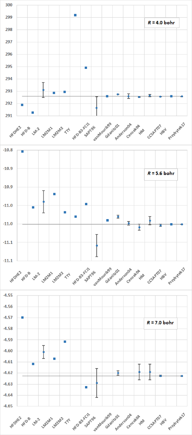
Figure 6: Comparison of ECG BO interaction energies $E_{\rm int}$ (in kelvin) at $R$ = 4.0, 5.6, and 7.0 bohr with those from selected earlier potentials. For empirical potentials (HFDHE2 and HFD-B), the sum of post-BO corrections was subtracted in each case. The energies are plotted as error bars from $E_{\rm int}-\sigma$ to $E_{\rm int}+\sigma$ (with dots at $E$) whenever uncertainty estimates $\sigma$ are available and as squares otherwise (for three cases at $R=7.0$ bohr, the energies are not available). The horizontal lines denote the positions of the BO energies calculated in Ref. 172. For acronyms, see the text.

progress in accuracy of predictions achieved since 1979. Empirical potentials dominated the field until the end of the 1980s; the two most widely used ones, HFDHE2 [206] and HFD-B, [207] developed by Aziz et al. The first really successful ab initio potential was LM-2 by Liu and McLean. [208] Those authors performed CI calculations and, by analyzing the configuration space and basis set convergence, obtained extrapolated interaction energies with estimated uncertainties (several versions of the LM-2 potential were proposed).

Aziz and Slaman [209] used the HFD-B functional form with refitted parameters to “mimic” the behavior of LM-2, of the unpublished ab initio data computed by Vos et al., [210] and of the small-$R$ Green-function Monte Carlo (GFMC) data [211] to obtain potentials denoted as LM2M1 and LM2M2, differing by assuming the smallest and largest LM-2 potentials well depths, respectively. The parameters of these potentials were not fitted directly to ab initio data, but chosen by trial and error to reproduce both theoretical data and measured quantities to within their error bars. The LM2M2 potential was considered to be the best helium potential until the mid-1990s, when purely ab initio calculations took the lead. Among the latter ones, TTY is a remarkably simple potential based on perturbation theory developed by Tang et al. [212] The HFD-B3-FCI1 potential was obtained by Aziz et al., [3] who used the HFD-B functional form with its original parameters adjusted so that the new potential runs nearly through the ab initio data points. These points were GFMC results of Ref. 211 and the FCI results of van Mourik and van Lenthe. [213] No uncertainties were assigned to HFD-B3-FCI1 and Fig. 6 shows that it was about as accurate as LM1LM2.

The SAPT96 potential [170, 171] opens an era of helium potentials based mostly on calculations with explicitly correlated functions. It was the first fully first-principles He₂ potential with reliable estimates of uncertainties. The potential was obtained using a two-level incremental strategy. The leading SAPT corrections (the complete first-order and the bulk of the second-order interaction energies) were computed using GTG basis sets. [214, 189, 191] The GTG-based variant of SAPT was developed in Refs. 215, 214, 216, 217, 218. Higher-order SAPT corrections were computed using the general SAPT program based on orbital expansions. [219, 220, 221, 222, 223] Large orbital basis sets including up to $g$-symmetry functions and midbond functions (placed between the nuclei) [224] were used. The remaining many-electron effects were computed using both SAPT based on FCI monomers, with summations to a very high order of perturbation theory (using He₂-specific codes), and supermolecular FCI calculations in small orbital basis sets. It is interesting to note that the errors of SAPT96 turned out to be completely dominated by the residual orbital (rather than GTG) contributions. For instance, at $R=5.6$ bohr, the orbital part constitutes only $-$1.81 K out of $-$11.00 K, but its error was $-$0.05 K out of the total SAPT96 error of $-$0.06 K. The underestimation of the uncertainties seen in Fig. 6 for $R=5.6$ bohr was entirely due to this issue. With an added retardation correction, SAPT96 was used (under the name of SAPT2) by Janzen and Aziz [225] to calculate properties of helium and found to be the most accurate helium potential at that time.

Van Mourik and Dunning [226] calculated CCSD(T) energies in basis sets up to daug-cc-pV6Z, CCSDT $-$ CCSD(T) differences in the daug-cc-pVQZ basis set, and FCI $-$ CCSDT differences in the daug-cc-pVTZ basis set. The CCSD(T) energies were CBS-extrapolated and then refined by adding a correction equal to the $R$-interpolated differences between highly accurate CCSD(T)-R12 results (available at a few distances in Ref. 227) and the obtained CBS limits. The CC-R12 methods are analogous to CC-GTG methods, but the explicit correlation factor enters linearly. [190]

Supermolecular ECG-based calculations for He₂ started to appear in the late 1990’s, [228, 229] and were initially aimed at providing upper bounds to the interaction energies (by subtracting essentially exact monomer energies), as the authors did not attempt to extrapolate their results to the CBS limits. Another application of explicitly correlated functions to the helium interaction was a series of papers by Gdanitz, [230, 231, 232] who used the multireference averaged coupled-pair functional method with linear $R_{12}$ factors, $R_{12}$-MR-ACPF. The extrapolated results from the last paper of the series, Ref. 232 (denoted “Gdanitz01” in Fig. 6), were among the most accurate results available at that time. However, the reported uncertainties were strongly underestimated at shorter distances (as much as 5 times at 5.6 bohr and 17 times at 4.0 bohr).

Another important series of papers was published by Anderson et al., [233, 234, 235] who reported quantum Monte Carlo energies with progressively reduced statistical uncertainties. Although these results were obtained only for a few internuclear distances, they represented very valuable benchmarks for mainstream electronic structure methods. In fact, until the publication of the CCSAPT07 potential, the result from Ref. 235, $-$10.998(5) K (see “Anderson04” in Fig. 6), was the most accurate value available at 5.6 bohr.

In Refs. 236, 237, a hybrid supermolecular ECG/orbital method was applied to the helium dimer. The bulk of the correlation effect on the interaction energy, at the CCSD level, was evaluated using GTG functions and the method developed in Refs. 238, 239, 240, 241, 242, 243, 244, 245, 246, 247, 248, 249. The nonlinear parameters were optimized at the MP2 level. The effects of noniterative triple excitations (the “(T)” contribution), i.e., the differences between CCSD(T) and CCSD energies, were calculated using large orbital basis sets (up to aug-cc-pV6Z with bond functions and daug-cc-pV6Z) and extrapolated to the CBS limits. Finally, the FCI corrections (differences between FCI and CCSD(T) energies) were obtained in basis sets up to aug-cc-pV5Z with bond functions and daug-cc-pV5Z, and also extrapolated. Results for three distances were reported in Ref. 237 (see “Cencek04” in Fig. 6).

Hurly and Mehl (HM) analyzed the best existing ab initio data for the helium dimer and created a new potential [5] representing a compromise based on uncertainties of existing data and their mutual agreement (for instance, as can be seen in Fig. 6, the result from Ref. 237 was used at $R$ = 7.0 bohr). The diagonal adiabatic corrections from Ref. 250 were added to the final potential, which was then used to calculate the second virial coefficient, viscosity, and thermal conductivity of helium.

The CCSAPT07 potential [180] based on the hybrid GTG/orbital method, published in 2007, was a significant improvement over the previous complete potential of this type, i.e., the SAPT96 potential. [170, 171] CCSAPT07 combined three different computational techniques, according to the criterion of the lowest uncertainty available for a given internuclear distance. Variational four-electron ECG calculations were used for $R\leq 3.0$ bohr and SAPT+FCI was employed for $R>6.5$ bohr. At intermediate distances, the hybrid supermolecular method developed in Refs. 236, 237 and described above provided the highest accuracy. Compared to Refs. 236, 237, several computational improvements were introduced, [179] resulting in significantly reduced uncertainties. The SAPT calculations [180] of CCSAPT07 followed the SAPT96 recipe, but also with larger basis sets and some computational improvements. The uncertainties of this potential were smaller than some effects that are neglected at the nonrelativistic BO level. Calculations of these effects will be discussed in Sec. III.3.2

Another highly accurate potential, by Hellmann, Bich, and Vogel (HBV), [251] appeared almost at the same time as CCSAPT07. Those authors used very large basis sets (up to daug-cc-pV8Z with added bond functions at the CCSD level, progressively smaller for higher levels of theory up to FCI) and CBS extrapolations. After augmenting the HBV potential with adiabatic, approximate relativistic, and retardation corrections, the authors used it to calculate thermophysical properties of helium. [252] However, the uncertainties of the HBV potential were not estimated, which restricts its usefulness. A direct accuracy comparison between the pure BO component of HBV and CCSAPT07 is now possible because of the much higher accuracy of the present-day benchmark energies, [172] and we performed such analysis using the values reported in the last column of Table 3 in Ref. 251. Out of 11 distances for which all three energies are available, the largest relative error (with respect to the results of Ref. 172), equal to 0.90%, occurs for the CCSAPT07 energy at 5.0 bohr, while the error of the HBV energy at this distance is only 0.48%. If one excludes this distance, which is close to where the helium potential crosses zero, and calculates the average relative error at the remaining distances, one obtains 0.007% for CCSAPT07 and 0.011% for HBV. Therefore, both potentials exhibit a similar level of accuracy.

The current most accurate nonrelativistic BO potential for the helium dimer was published in Ref. 172; see Ref. 188 for details of these calculations. The significant improvement over all previous potentials was achieved by a combination of three factors. First, a pure ECG approach was used, i.e., with all four electrons explicitly correlated and no contributions calculated with orbital methods. Indeed, the residual errors of the older hybrid ECG-orbital potentials, SAPT96 [170, 171] and CCSAPT07, [180] were dominated by insufficient basis set saturation of the relatively small orbital contributions. Second, the use of the monomer contraction method, [184, 253] i.e., the use of the product of helium atoms wave functions as one of the functions in the basis set, dramatically improved the energy convergence with respect to the ECG expansion size. Furthermore, an optimized contraction [254, 199] replacement of the simple product of monomer wave functions by a more compact sum of four-electron functions optimized for two noninteracting helium atoms, reduced the computational cost at the nonlinear parameters optimization stage. Third, a near-complete optimization of nonlinear parameters in large basis set expansions was possible due to this reduced cost and due to other improvements of the optimization algorithm.

III.3.2 Physical effects beyond the nonrelativistic Born–Oppenheimer level

With the small uncertainties of the CCSAPT07 BO potential, [180] it became clear that a further reduction of uncertainties required inclusion of post-BO effects. The first calculation of all relevant such effects for the whole potential-energy curve was presented in Ref. 133 and later improved in Refs. 6, 172, 7. Some post-BO effects for the whole curve were included even earlier in Refs. 251, 252, but this work omitted non-negligible two-electron terms in the $\alpha^{2}$ relativistic and $\alpha^{3}$ QED corrections. The current helium dimer potentials at the post-BO level include the diagonal adiabatic correction, relativistic corrections (earlier computed in Ref. 184, but for the minimum separation only), the QED correction, and the retardation effect (a long-range QED correction)

$$V(R)=V_{\rm BO}+V_{\rm ad}+V_{\rm rel}+V_{\rm QED}+V_{\rm ret}.$$

In Refs. 133, 6, all the post-BO corrections were computed in the supermolecular way as the differences of expectation values of appropriate operators with the dimer and monomer wave functions, except at the CCSD(T) level, see below. The kinetic energy of the nuclei operator was used for the adiabatic correction, the $\alpha^{2}$ Breit–Pauli operator [197] for the relativistic correction, and the $\alpha^{3}$ QED operator [255] for the QED correction. In the latter case, one approximation was made in the operator. In the term

$$-\frac{8\alpha}{3\pi}\hat{D}_{1}\ln k_{0},\\$$

with

$$\hat{D}_{1}=\frac{\pi}{2}\,\alpha^{2}\sum_{I}\sum_{i=1}^{4}Z_{I}\delta({\bm{r}}_{i}-{\bm{r}}_{I}),$$

where the sum over $I$ is over the nuclei, the value of $\ln k_{0}$ should be computed for each $R$, but instead a constant value was taken, equal to the value of $\ln k_{0}$ for the helium atom. Thus, the $R$ dependence originated entirely from that of the $\hat{D}_{1}$ operator.

All corrections were computed using both four-electron ECG basis sets and orbital basis sets (except for the Araki–Sucher part of the QED operator where only ECG functions were used). The calculations with smaller uncertainties were selected for the final potential. Orbital calculations were performed using a combination of CCSD(T) and FCI approaches or FCI alone. For the adiabatic correction, only FCI was used. The calculations of the average values of the operators listed above with ECG and FCI wave functions are straightforward (although regularization techniques have to be used for singular operators). However, the CCSD(T) wave function needed to compute expectation values is not available (not defined) and instead the CCSD(T) linear response method was used, [256] i.e., first-order analytic derivatives of CCSD(T) energy (with the perturbation operator included) were computed. The retardation effects of long-range electromagnetic interactions were computed from the Casimir–Polder expression [257] dependent on the dynamic polarizability of the helium atom.

Calculations of Ref. 172 dramatically improved the accuracy of the helium dimer potential with uncertainties reduced by an order of magnitude compared to those of Refs. 180, 133. As already discussed, the main improvement was due to the use of larger and better optimized ECG wave functions at the nonrelativistic BO level of theory for all $R\leq 9$ bohr. Accuracy of the adiabatic and relativistic corrections was also improved by using larger basis sets than in Refs. 133, 6. A major theoretical advance was the calculation of the properties of the very weakly bound state of He₂ (the so-called halo state) with full inclusion of nonadiabatic effects.

The accuracy of relativistic and QED contributions was further improved in Ref. 7. The contributions to the interaction energy at the van der Waals minimum are presented in Table 2. Clearly, with the uncertainty of the BO contribution of $0.00020$ K, all the included post-BO contributions are relevant, except for the retardation contribution, but this contribution does become important at very large separations. [185] One can also see that uncertainties of the adiabatic, relativistic, and QED terms are almost negligible compared to the uncertainty of the BO term. The potential of Ref. 7 was used to compute the second virial coefficient and the second acoustic virial coefficient of helium.

Table 2: Contributions to the interaction energy of helium dimer (in K) at the van der Waals minimum at $R=5.6$ bohr. Results from Refs. 172, 7.

Contribution	Value	Uncertainty
$V_{\rm BO}$	$-11.00071$	0.00020
$V_{\rm ad}$	$-0.0089048$	0.0000097
$V_{\rm rel}$	$0.0153911$	0.0000154
$V_{\rm QED}$	$-0.0013327$	0.0000018
$V_{\rm ret}$	$0.000012$

III.4 Nonadditive helium potentials

In any fluid, the total interaction energy includes terms beyond pairwise-additive interactions between monomers. These so-called nonadditive contributions begin with three-body nonadditive terms defined as the part of the trimer interaction energy that cannot be recovered by the sum of two-body interaction. The additive and nonadditive interactions form a series called the many-body expansion of interaction energy. Fortunately, for all fluids consisting of monomers interacting via noncovalent forces, this expansion converges very fast and usually it is sufficient to limit calculation to two- and three-body terms. For a review of the many-body expansion, see Ref. 258. For metrology purposes, the three-body potential is needed to calculate the third virial coefficient.

A pairwise-nonadditive potential for helium was developed in Ref. 259 and improved in Ref. 134. In the earlier work, two independent potentials were obtained. One was based on three-body SAPT [260, 261, 262, 263, 264] and the other on the supermolecular CCSD(T) approach. Orbital basis sets up to aug-cc-pV5Z were used. The two potentials were in very good agreement. In Ref. 134, the CCSD(T) potential was improved by calculating the FCI correction in an incremental approach and increasing the number of grid points, with CCSD(T) values taken from Ref. 259 except for the new grid points. Near the minimum of the total potential, the three-body contribution is only $-0.0885$ K, which should be compared to the total interaction energy of about $33$ K, but the three-body contribution is much larger than the uncertainty resulting from the two-body term, which is $0.0006$ K. The uncertainty of the three-body term at the minimum of the total potential was estimated to be $0.002$ K.

Recently, the three-body potential for helium was further improved [265] by adding relativistic and nuclear-motion corrections, using a new set of correlation-consistent basis sets specifically developed for helium atoms, [172] and developing an improved analytic form of the potential at large distances. In particular, new terms were developed for the case when two atoms remain close while the third is progressively more distant. These refinements resulted in a reduction of the uncertainty by a factor of about $5$ overall. In particular, the uncertainty at the minimum was reduced to $0.5$ mK, a factor of 4 smaller than that of the previous work. [265]

III.5 Heavier noble-gas atoms

While theory is superior to experiment for the helium atom and helium clusters, this is not the case for neon, and even more so for argon. The simple reason is the number of electrons: 2, 10, and 18, respectively. While for the helium atom and small helium clusters the $N$-electrons explicitly correlated bases can reach ppm or smaller uncertainties, and FCI calculations can be performed in fairly large bases, for the neon atom neither type of calculation can be performed in large enough bases to get meaningful results. To quantify this statement, let us examine the most accurate calculations for the neon dimer, [112] see Table 3. The calculations at the CCSD(T) level of theory were performed in the largest available basis sets: modified daug-cc-pV8Z with bond functions. The uncertainty of this result is about 200 ppm, which is only 10 times larger than the 20 ppm uncertainty of the He₂ BO interaction energy. The main problem comes from higher excitations. As Table 3 shows, the uncertainties of the consecutive terms increase, and the final $\Delta$(P) contribution increases the uncertainty of the total value to about 1000 ppm. The increase of uncertainties is due to the use of smaller and smaller basis sets as the number of excitations increases: at the CCSDTQ(P) level of theory only the daug-cc-pVDZ basis set could be used. Even worse, the values of the consecutive contributions do not seem to converge well, so it is not really possible to estimate the errors due the truncation of theory at the CCSDTQ(P) level. FCI calculations cannot currently be performed even in bases of the size used for CCSDTQ(P), so FCI is not a solution either.

Table 3: Contributions to the interaction energy of neon dimer (in K) at the van der Waals minimum, $R=3.1$ Å, from Ref. 112. (P) denotes noniterated quintuple excitations.

Contribution	${\rm Value}$	Uncertainty
CCSD(T)	$-41.3301$	0.0100
$\Delta$T	$0.5730$	0.0115
$\Delta$Q	$-0.1645$	0.0121
$\Delta$(P)	$0.1179$	0.0589

Similar calculations at the limits of the available technology were performed for Ar₂ in Ref. 266 (see also earlier calculations [267] with accurate treatment of very small $R$). The final value of the interaction energy at the minimum is ($-142.86\pm 0.46$) K. Thus, the estimated uncertainty is 3000 ppm (or 0.3%). The uncertainty does not include an estimate of effects beyond CCSDTQ since in the case of Ar₂ the highest-excitation contribution was only 0.12 K. The results of Ref. 112 indicate, however, that the post-CCSDTQ contribution may be not negligible.

The first first-principles three-body potential for argon was developed in Ref. 261 using three-body SAPT. It was then used to compute the third virial coefficient of argon [139] and to simulate vapor-liquid equilibria. [147] An improved three-body potential for argon was developed in Ref. 268 using the CCSDT(Q) level of theory and including correlation effects. Uncertainties of the potential were estimated. This work also computed the third virial coefficient, getting good overall agreement with experiments. In particular, in some regions of temperature, theoretical values have smaller uncertainties than experiment and comparisons with theory allow evaluation of different experiments. When the experimental data were refitted by a new model that included an approximate fourth virial coefficient, the agreement with theory improved, which can be considered to be a validation of the new model. The work of Ref. 268 shows that despite limitations of accuracy, for some properties theory may provide information relevant for metrology experiments and its accuracy may be competitive to experimental accuracy.

III.6 Magnetic susceptibility

Magnetic susceptibilities of atoms are relevant for RIGT (see Eq. (11)). In general, the magnetic susceptibility is several orders of magnitude smaller than the electric susceptibility. Therefore, it is usually sufficient to compute it at the BO level of theory. The contribution of relativistic effects can be estimated using perturbation theory. These corrections can also be considered as an additional contribution to the uncertainty of the calculation.

For the helium atom, the magnetic susceptibility was computed quite some time ago. [74] Accurate calculations for neon [59, 60] and argon [61] were performed only recently.

IV From Electronic Structure to Thermophysical Properties

Virial expansions are exact results from quantum statistical mechanics which enable a systematically improvable evaluation of various thermophysical properties as a power series in density starting from the ideal-gas reference system. The coefficients appearing in the $N$-th term of the series can be computed from the knowledge of the interaction of clusters of $N$ particles.

In the case of the equation of state – i.e., the expansion of the pressure $p$ as a function of density $\rho$ – one obtains Eq. (7) [269, 270] together with rigorous expressions for the virial coefficients $B(T)$, $C(T)$, $D(T)$, etc., which turn out to be functions of temperature only and are given by

$$\frac{B(T)}{N_{\mathrm{A}}} = -\frac{1}{2V}\left(Z_{2}-Z_{1}^{2}\right)$$ (27)

$$\frac{C(T)}{N_{\mathrm{A}}^{2}} = \frac{\left(Z_{2}-Z_{1}^{2}\right)^{2}}{V^{2}}-\frac{1}{3V}\left(Z_{3}-3Z_{2}Z_{1}+2Z_{1}^{3}\right)$$ (28)

$$\frac{D(T)}{N_{\mathrm{A}}^{3}} = -\frac{Z_{4}-4Z_{3}Z_{1}-3Z_{2}^{2}+12Z_{2}Z_{1}^{2}-6Z_{1}^{4}}{8V}+$$ (29)

$$\frac{3(Z_{2}-Z_{1}^{2})(Z_{3}-3Z_{2}Z_{1}+2Z_{1}^{3})}{2V^{2}}-$$

$$\frac{5(Z_{2}-Z_{1}^{2})^{3}}{2V^{3}},$$

with

$$\frac{Z_{N}}{N!}=\frac{Q_{N}(V,T)~{}V^{N}}{Q_{1}(V,T)^{N}},$$ (30)

where $Q_{N}(V,T)$ is the partition function of a system of $N$ particles evaluated in the canonical ensemble and $N_{\mathrm{A}}$ is the Avogadro constant. These partition functions can be calculated once the interaction potential $U_{N}(\mathbf{x}_{1},\ldots,\mathbf{x}_{N})$ among $N$ particles is known; the potential is generally expressed as

$$U_{N}=\sum_{i<j}^{N}u_{2}(\mathbf{x}_{i},\mathbf{x}_{j})+\sum_{i<j<k}^{N}u_{3}(\mathbf{x}_{i},\mathbf{x}_{j},\mathbf{x}_{k})+\ldots,$$ (31)

where $u_{2}$ is the pair potential, $u_{3}$ is the non-additive contribution to the three-body potential, and so on. In Eq. (31) we specialized to the case of atomic systems, which will be principal topic of this review; in this case $\mathbf{x}_{i}$ represent the position of the $i$-th atom. In the case of molecules, which we will discuss in Sec. V, the various potentials appearing in Eq. (31) depend also on coordinates $\mathbf{y}_{i}$ that describe the intramolecular configuration of molecule $i$. In particular, a single-body potential $u_{1}(\mathbf{y}_{1})$ will also appear in Eq. (31). The potentials and their uncertainties can be computed from first principles using the methods described in Sec. III. The most general expression for $Q_{N}(V,T)$ in quantum statistical mechanics is given by

$$Q_{N}(V,T) = {\sum_{i}}^{\prime}\langle i|\mathrm{e}^{-\beta H_{N}}|i\rangle$$ (32)

$$= \frac{1}{N!}\sum_{j=1}^{N!}\sum_{i}\langle i|\mathrm{e}^{-\beta H_{N}}{\cal P}_{j}|i\rangle,$$ (33)

where $\beta=(k_{\mathrm{B}}T)^{-1}$ and the primed sum in Eq. (32) is on a complete set of states $|i\rangle$ of the $N$-body Hamiltonian $H_{N}$ with the proper symmetry upon particle exchange due to the bosonic or fermionic nature of the particles involved. Equation (33) is an equivalent expression where the sum over the states has no restriction on the symmetry and the operators ${\cal P}_{j}$ represent the $j$-th permutation of particles in the Hilbert space, including the sign of the permutation in the case of fermions. The latter expression will be the most convenient when discussing the path-integral Monte Carlo approach for the calculation of virial coefficients. [271, 272] The non-relativistic $N$-body Hamiltonian is conveniently written as

$$H_{N}=\sum_{i=1}^{N}\frac{\bm{\pi}_{i}^{2}}{2m_{i}}+U_{N}\equiv T_{N}+U_{N},$$ (34)

where we have introduced the momentum operator $\bm{\pi}_{i}$ and mass $m_{i}$ for the $i$-th particle and the second equality defines the $N$-body kinetic energy $T_{N}$.

Virial expansions of the form of Eq. (7) have been derived for several other quantities measured by the gas-based devices described in Sec. II: the speed of sound in Eq. (1), the dielectric constant in Eq. (9), and the index of refraction in Eq. (11). The coefficients appearing in Eq. (1) are given by [273]

$$\beta_{\mathrm{a}}(T) = 2B+2(\gamma_{0}-1)T\frac{\mathrm{d}B}{\mathrm{d}T}+\frac{(\gamma_{0}-1)^{2}}{\gamma_{0}}T^{2}\frac{\mathrm{d}^{2}B}{\mathrm{d}T^{2}}$$ (35)

$$RT\gamma_{\mathrm{a}}(T) = \left(\frac{\gamma_{0}-1}{\gamma_{0}}Q^{2}-\beta_{\mathrm{a}}(T)B(T)\right)+\frac{2\gamma_{0}+1}{\gamma_{0}}C+$$ (36)

$$\frac{\gamma_{0}^{2}-1}{\gamma_{0}}T\frac{\mathrm{d}C}{\mathrm{d}T}+\frac{(\gamma_{0}-1)^{2}}{2\gamma_{0}}T^{2}\frac{\mathrm{d}^{2}C}{\mathrm{d}T^{2}},$$

where the quantity $Q$ is

$$Q=B+(2\gamma_{0}-1)T\frac{\mathrm{d}B}{\mathrm{d}T}+(\gamma_{0}-1)T^{2}\frac{\mathrm{d}^{2}B}{\mathrm{d}T^{2}}.$$ (37)

The density expansion of the dielectric constant $\varepsilon_{\mathrm{r}}$ is generally given as a generalization of the Clausius–Mossotti equation in one of the two equivalent forms given by Eqs. (8) and (9). Until recently, derivations for the coefficients appearing in these equations would agree on the expression for the second dielectric virial coefficient, $B_{\varepsilon}$, but differ in the case of the higher-order coefficients. [274, 275, 276] A systematic review of the dielectric expansion showed that the correct expressions are [276, 200]

$$A_{\varepsilon} = \frac{4\pi\alpha_{1}}{3}N_{\mathrm{A}}$$ (38)

$$B_{\varepsilon}(T) = \frac{2\pi k_{\mathrm{B}}T}{3V}N_{\mathrm{A}}^{2}\frac{\partial^{2}Z_{2}(V,T,E_{0})}{\partial E_{0}^{2}}$$ (39)

$$C_{\varepsilon}(T) = -\frac{2\pi k_{\mathrm{B}}TN_{\mathrm{A}}^{3}}{3}\left[\frac{2}{V^{2}}\left(\frac{\partial Z_{2}}{\partial E_{0}}\right)^{2}+\frac{2(Z_{2}-V^{2})}{V^{2}}\frac{\partial^{2}Z_{2}}{\partial E_{0}^{2}}\right.$$ (40)

$$\left.-\frac{1}{3V}\left(\frac{\partial^{2}Z_{3}}{\partial E_{0}^{2}}-3V\frac{\partial^{2}Z_{2}}{\partial E_{0}^{2}}\right)\right],$$

where $\alpha_{1}$ is the atomic polarizability and the functions $Z_{N}$ are given by expressions similar to Eq. (30), where the interaction Hamiltonian among the constituent particles of Eq. (34) is extended with two terms in order to include the effect of the interactions of the dipole moment and the electronic polarizability of the system with an external electric field of magnitude $E_{0}$. In Eqs. (38)–(40), the derivatives are to be evaluated at $E_{0}=0$. The two additional terms in the Hamiltonian are

$$H^{\mathrm{dip}}_{N} = -\left(\sum_{i=1}^{N}\mathbf{m}_{1}(i)+\sum_{i<j}\mathbf{m}_{2}(i,j)+\right.$$ (41)

$$\left.\sum_{i<j<k}\mathbf{m}_{3}(i,j,k)+\ldots\right)\cdot\mathbf{E}_{0}$$

$$H^{\mathrm{pol}}_{N} = -\frac{1}{2}\mathbf{E}_{0}\cdot\left(\sum_{i=1}^{N}\bm{\alpha}_{1}(i)+\sum_{i<j}\bm{\alpha}_{2}(i,j)+\right.$$ (42)

$$\left.\sum_{i<j<k}\bm{\alpha}_{3}(i,j,k)+\ldots\right)\cdot\mathbf{E}_{0},$$

where $\mathbf{m}_{n}$ and $\bm{\alpha}_{n}$ are the (non-additive) dipole moments and the (non-additive) electronic polarizabilities of a system of $n$ particles. In the case of atoms, $\mathbf{m}_{1}$ and $\mathbf{m}_{2}$ are both zero, but a system of three particles has, in general, $\mathbf{m}_{3}\neq 0$. [277, 278]

An expression analogous to the Clausius–Mossotti equation (9) was derived by Lorentz and Lorenz for the refractive index $n$ and is reported in Eq. (11). The Lorentz–Lorenz equation (11) is relevant to those experiments where the refractive index is measured by optical methods. In this case, the refractive virial coefficients are a function of the angular frequency $\omega$ of the electromagnetic radiation as well as the temperature. Usually, the frequency dependence is approximated as a power-law expansion of the form

$$B_{\mathrm{R}}(T)=B_{\varepsilon}+\omega^{2}B_{\mathrm{R}}^{(2)},$$ (43)

where $B_{\mathrm{R}}^{(2)}$ depends on the interaction-induced Cauchy moment $\Delta S(-4)$. [279]

IV.1 Classical limit

Although the focus of this review is on calculations with no uncontrolled approximation, let us briefly discuss the classical limit of the approach we have outlined. Classical expressions can be computed relatively easily, and provide a useful high-temperature check for the more involved calculations described below.

Since quantum exchange effects are absent in classical mechanics, the only term that remains in Eq. (33) is the one corresponding to the identity permutation, giving rise to the “correct Boltzmann counting” factor of $1/N!$ in the partition functions. [270] In the same limit, the kinetic term in the Hamiltonian (34) commutes with the potential energy $U_{N}$ as well as with $H^{\mathrm{dip}}_{N}$ and $H^{\mathrm{pol}}_{N}$. Its contribution can be integrated exactly, resulting in a factor of the form $V^{N}/\Lambda_{m}^{3N}$ where $\Lambda_{m}=h/\sqrt{2\pi mk_{\mathrm{B}}T}$ is the thermal de Broglie wavelength of the atoms under consideration. Putting all of this together, one obtains

$$Z_{N}^{[\mathrm{class}]}(V,T,E_{0})=\int\mathrm{e}^{-\beta\left(U_{N}+H^{\mathrm{dip}}_{N}+{H^{\mathrm{pol}}}^{\prime}_{N}\right)}~{}\mathrm{d}\mathbf{X}_{N},$$ (44)

where the ${H^{\mathrm{pol}}}^{\prime}_{N}$ is the same as Eq. (42), but without the terms corresponding to $\bm{\alpha}_{1}$. Additionally, we have denoted by $\mathrm{d}\mathbf{X}_{N}$ the integration element in the space of all the coordinates needed to describe a system of $N$ atoms, e.g., the Cartesian coordinates $\mathbf{x}_{1},\ldots,\mathbf{x}_{N}$. Since the system is translationally invariant, the integration produces a factor of $V$ with the understanding that one particle, usually labelled as $1$, is fixed at the origin of the coordinate system. Using rotational invariance, one can further write for the integration elements

$$\mathrm{d}\mathbf{X}_{2} = V~{}4\pi r_{12}^{2}~{}\mathrm{d}r_{12}$$ (45)

$$\mathrm{d}\mathbf{X}_{3} = V~{}8\pi^{2}(r_{12}r_{13})^{2}~{}\mathrm{d}r_{12}\mathrm{d}r_{13}\mathrm{d}\cos\theta_{23}$$ (46)

$$\mathrm{d}\mathbf{X}_{4} = V~{}8\pi^{2}(r_{12}r_{13}r_{14})^{2}\times$$ (47)

$$\mathrm{d}r_{12}\mathrm{d}r_{13}\mathrm{d}r_{14}\mathrm{d}\cos\theta_{23}\mathrm{d}\cos\theta_{14}\mathrm{d}\phi,$$

where we have denoted by $r_{ij}=|\mathbf{r}_{ij}|=|\mathbf{x}_{i}-\mathbf{x}_{j}|$ and $\theta_{ij}$ the angle between the vectors $\mathbf{r}_{i1}$ and $\mathbf{r}_{j1}$. In Eq. (47) the angle $\phi$ is the polar angle corresponding to the vector $\mathbf{r}_{14}$ in spherical coordinates.

Using Eqs. (27), (35), and (39), one obtains the classical expressions

$$B_{\mathrm{cl}} = -2\pi N_{\mathrm{A}}\int\left(\mathrm{e}^{-\beta U_{2}(r_{12})}-1\right)~{}r_{12}^{2}\mathrm{d}r_{12}$$ (48)

$$\beta_{\mathrm{a,cl}} = -2\pi N_{\mathrm{A}}\int r_{12}^{2}\left[2\left(\mathrm{e}^{-\beta U_{2}}-1\right)+\right.$$ (49)

$$2(\gamma_{0}-1)\beta U_{2}\mathrm{e}^{-\beta U_{2}}+$$

$$\left.\frac{(\gamma_{0}-1)^{2}}{\gamma_{0}}\beta U_{2}(\beta U_{2}-2)\mathrm{e}^{-\beta U_{2}}\right]\mathrm{d}r_{12}$$

$$B_{\varepsilon,\mathrm{cl}} = \frac{8\pi^{2}}{3}N_{\mathrm{A}}^{2}\int\Delta\alpha_{2}(r_{12})\mathrm{e}^{-\beta U_{2}(r_{12})}\mathrm{d}r_{12},$$ (50)

for the second density, acoustic, and dielectric second virial coefficient, respectively. In Eq. (50) we have defined $\Delta\alpha_{2}=\frac{1}{3}\mathrm{Tr}(\bm{\alpha}_{2})$, which is the average of the interaction-induced pair polarizability. The classical expression for $B_{\mathrm{R,cl}}^{(2)}$ is analogous to Eq. (50), where $\Delta\alpha_{2}$ is substituted by the Cauchy moment $\Delta S(-4)$.

In the same way, one can derive expressions for the classical limit of the third density, acoustic, and dielectric virial coefficients using Eqs. (28), (36), and (40). After some lengthy, but straightforward, evaluation, they turn out to be

$$C_{\mathrm{cl}} = -\frac{8\pi^{2}}{3}N_{\mathrm{A}}^{2}\int\left[\mathrm{e}^{-\beta U_{3}}-\sum_{i<j}\mathrm{e}^{-\beta U_{2}(r_{ij})}+2-3(\mathrm{e}^{-\beta U_{2}(r_{12})}-1)(\mathrm{e}^{-\beta U_{2}(r_{13})}-1)\right]~{}\mathrm{d}\Omega_{3}$$ (51)

$$C_{\varepsilon,\mathrm{cl}} = \frac{16\pi^{2}}{9}N_{\mathrm{A}}^{3}\int\left[\left(\frac{\beta|\mathbf{m}_{3}|^{2}}{3}+\Delta\alpha_{3}\right)\mathrm{e}^{-\beta U_{3}}-\sum_{i<j}\Delta\alpha_{2}(r_{ij})\mathrm{e}^{-\beta U_{2}(r_{ij})}-\right.$$ (52)

$$\left.6\left(\mathrm{e}^{-\beta U_{2}(r_{12})}-1\right)\Delta\alpha_{2}(r_{13})\mathrm{e}^{-\beta U_{2}(r_{13})}\right]~{}\mathrm{d}\Omega_{3},$$

where $\mathrm{d}\Omega_{3}=(r_{12}r_{13})^{2}~{}\mathrm{d}r_{12}\mathrm{d}r_{13}\mathrm{d}\cos\theta_{23}$, $r_{23}=\sqrt{r_{12}^{2}+r_{13}^{2}-2r_{12}r_{13}\cos\theta_{23}}$, and $\Delta\alpha_{3}=\frac{1}{3}\mathrm{Tr}(\bm{\alpha}_{3})+\displaystyle\sum_{i<j}\Delta\alpha_{2}(r_{ij})$. The classical expression for the third acoustic virial coefficient $\gamma_{\mathrm{a}}$ is more involved and is given in Appendix A.

IV.2 Quantum calculation of virial coefficients

The classical approach can be expected to be valid when $\Lambda/\sigma\ll 1$, where $\sigma$ can be taken as the size of the hard-core repulsive region of atoms (which is around $0.3$ nm for the noble gases): this implies that the classical formulae will be asymptotically valid for high temperatures and heavy atoms. However, in the case of helium this approximation is too drastic even at room temperature.

The inclusion of quantum effects in the calculation of virial coefficients (density, acoustic, or dielectric) requires evaluating the $N$-body partition functions $Q_{N}$ of Eq. (32) in a quantum framework. A straightforward approach would be to consider in Eq. (32) the eigenstates $|i\rangle$ of the $N$-body Hamiltonian, $H_{N}|i\rangle=E_{i}|i\rangle$, so that Eq. (32) becomes a simple sum. To the best of our knowledge, this method has been demonstrated to date only in the case of the second dielectric virial coefficient. [73]

In the case of $Q_{2}$ (which enables the calculation of virial coefficients of order 2), a very fruitful approach dating back to the late 1930s [280, 269] is to rewrite it as the sum of three terms: one depending on the bound-state energies, one depending on the phase shifts of the scattering states, and one depending on the bosonic or fermionic nature of the atoms involved. The expression of $B(T)$ becomes then

$$B(T) = B_{\mathrm{th}}(T)+B_{\mathrm{bound}}(T)+B_{\mathrm{xc}}(T)$$ (53)

$$B_{\mathrm{th}}(T) = -\frac{N_{\mathrm{A}}\Lambda_{\mu}^{3}}{\pi}\int\mathrm{e}^{-\beta E}S(E)~{}\beta\mathrm{d}E$$ (54)

$$S(E) = \sum_{l}(2l+1)f(I,l)\delta_{l}(E)$$ (55)

$$B_{\mathrm{bound}}(T) = -\frac{N_{\mathrm{A}}\Lambda_{\mu}^{3}}{2}\sum_{l,n}(2l+1)f(I,l)\left(\mathrm{e}^{-\beta E_{nl}^{\mathrm{bound}}}-1\right)$$ (56)

$$B_{\mathrm{xc}}(T) = -N_{\mathrm{A}}\frac{(-1)^{2I}}{2I+1}\frac{\Lambda_{\mu}^{3}}{16},$$ (57)

where $\mu$ is the reduced mass of the pair of atoms considered, $E_{nl}^{\mathrm{bound}}$ is the energy of the $n$-th bound state with relative angular momentum $l$, and $f(I,l)=1+(-1)^{2I+l}/(2I+1)$ with $I$ the nuclear spin in the case of identical atoms (the case of different atoms can be recovered by letting $I\to\infty$). The quantity $\delta_{l}(E)$ in Eq. (55) is the absolute scattering phase shift for two particles with relative energy $E$ and angular momentum $l$. Absolute phase shifts are continuous functions of $E$ that tend, in the limit of $E\to 0$, to $\pi$ times the number of bound states at angular momentum $l$. With the advent of electronic computers, the use of Eqs. (53) to (57) enabled the calculation of accurate numerical values [281, 282] and it is still the most efficient way to compute the second virial coefficient of atomic species. [6, 7] One important benefit of this method is that once the energies of all the bound states have been computed and phase shifts are known for a sufficiently high number of total angular momenta and scattering energies, the values of $B(T)$ and its derivatives, and hence $\beta_{\mathrm{a}}(T)$, can be easily computed at all temperatures; knowledge of the collision-induced pair polarizability also enables the calculation of $B_{\varepsilon}$. [73] Additionally, transport properties such as the viscosity and the thermal conductivity – see Sec. IV.6 below – can be computed in a straightforward manner.

Unfortunately, this approach cannot be easily extended to higher-order coefficients. Some attempts in this direction were made in the 1960s, [283, 284] but all of them required the introduction of some uncontrolled approximations and were not developed to take into account the non-additive parts of the many-body potential.

IV.2.1 Path integral approach

At the same time, the path-integral approach to quantum statistical mechanics [271] was shown by Fosdick and Jordan to provide a systematic way to compute virial coefficients of any order without any uncontrolled approximation. [285, 286] The path-integral formulation is based on a controlled approximation of the exponential of the $N$-body Hamiltonian, that is

$$\mathrm{e}^{-\beta H_{N}} = \left(\mathrm{e}^{-\beta(T_{N}+U_{N})/P}\right)^{P}$$ (58)

$$\simeq \left(\mathrm{e}^{-\beta T_{N}/P}\mathrm{e}^{-\beta U_{N}/P}\mathrm{e}^{-\beta O/P}\right)^{P},$$ (59)

where

$$O=\frac{\beta^{2}\hbar^{2}}{24P^{2}m}\sum_{i=1}^{N}|\nabla_{i}U_{N}|^{2}.$$ (60)

Equation (59) is the Li–Broughton expansion of the exponential of the sum, [287] which was independently discovered by Kono et al. [288] based on an initial idea by Takahashi and Imada. [289] It can be shown that Eq. (59) becomes an exact equality in the case $P\to\infty$, although in practice satisfactory convergence is reached for a finite value of the parameter $P$. Actually, Eq. (59) becomes an equality in the $P\to\infty$ limit also when $O$ is omitted in Eq. (59) (this is the original Trotter–Suzuki approach), although in this case convergence is attained at higher values of $P$; this approach is called the primitive approximation, [272] and, for the sake of simplicity, will be used throughout this review.

The path-integral approach is obtained by using Eq. (59) in Eq. (33) and inserting $P-1$ additional completeness relations between the $P$ factors in Eq. (59). Additionally, one uses as a complete set the (generalized) position eigenstates $|i\rangle=|\mathbf{X}_{N}^{(1)}\rangle$, where we have included a superscript $(1)$ for later convenience. In this case, the sum over $i$ in Eq. (33) becomes an integral over the $3N$ coordinates $\mathbf{X}_{N}^{(1)}$ and the $P-1$ completeness relations can be written as

$$\mathbf{1}=\int|\mathbf{X}_{N}^{(k)}\rangle\langle\mathbf{X}_{N}^{(k)}|~{}\mathrm{d}\mathbf{X}_{N}^{(k)},$$ (61)

with $k=2,\ldots,P-1$. Notice that in this case the effect of the permutation operators ${\cal P}_{j}$ is to exchange atomic coordinates in the rightmost ket. For example, if ${\cal P}(12)$ denotes the permutation of particles $1$ and $2$ (assumed to be bosons), one has

$${\cal P}(12)|\mathbf{x}_{1}^{(1)},\mathbf{x}_{2}^{(1)},\ldots,\mathbf{x}_{N}^{(1)}\rangle=|\mathbf{x}_{2}^{(1)},\mathbf{x}_{1}^{(1)},\ldots,\mathbf{x}_{N}^{(1)}\rangle.$$ (62)

Let us first proceed assuming that ${\cal P}$ is the identity permutation (that is, we are considering Boltzmann statistics; this approximation is essentially exact for $T\gtrsim 10$ K even in the case of helium) and the case of density virials of pure species (so that our Hamiltonian is given by Eq. (34) with $m_{i}=m$). The operators $U_{N}$ (and, if needed, $O$) of Eq. (59) are diagonal in the position basis. The matrix elements of the exponential of the kinetic energy operators can be calculated exactly [290] and are given by

$$\langle\mathbf{x}^{(k+1)}_{i}|\mathrm{e}^{-\frac{\beta\bm{\pi}_{i}^{2}}{2mP}}|\mathbf{x}^{(k)}_{i}\rangle=\frac{P^{3/2}}{\Lambda^{3}}\exp\left(-\frac{\pi P}{\Lambda^{2}}\left|\mathbf{x}^{(k+1)}_{i}-\mathbf{x}^{(k)}_{i}\right|^{2}\right),$$ (63)

so that $Z_{N}$ can be written as

$$Z_{N}=\int\mathrm{e}^{-\beta\overline{U_{N}}}\prod_{i=1}^{N}F_{i}\prod_{k=1}^{P}\mathrm{d}\mathbf{X}_{i}^{(k)},$$ (64)

where

$$\overline{U_{N}} = \frac{1}{P}\sum_{k=1}^{P}U_{N}(\mathbf{X}_{N}^{(k)})$$ (65)

$$F_{i} = \Lambda^{3}\left(\frac{P^{3/2}}{\Lambda^{3}}\right)^{P}\exp\left(-\frac{\pi P}{\Lambda^{2}}\sum_{k=1}^{P}\Delta{\mathbf{r}_{i}^{(k)}}^{2}\right)$$ (66)

$$\Delta{\mathbf{r}_{i}^{(k)}}^{2} \equiv \left|\mathbf{x}_{i}^{(k+1)}-\mathbf{x}_{i}^{(k)}\right|^{2},$$ (67)

with the understanding that $\mathbf{x}_{i}^{(P+1)}=\mathbf{x}_{i}^{(1)}$. Equations (64)–(66), which correspond exactly (in the $P\to\infty$ limit) to the original quantum statistical formulation, can be interpreted as the partition function of a classical system. [290] For each of the original $N$ particles of coordinates $\mathbf{x}_{i}^{(1)}$, one has introduced $P-1$ copies of coordinates $\mathbf{x}_{i}^{(k)}$, which, as one can see from Eq. (66), are connected via harmonic potentials. The equivalent classical system is then made by $N$ ring polymers of $P$ monomers each. As shown by Eq. (65), these polymers interact with the original potential averaged over all the monomers. It can be shown that the functions $F_{i}$ of Eq. (66) represent probability distributions. [291] Although they are not Gaussian probabilities, because of the ring-polymer condition $\mathbf{x}_{i}^{(P+1)}=\mathbf{x}_{i}^{(1)}$, they can be sampled exactly using an interpolation formula due to Levy [285, 286] (also known as “the Brownian bridge”). The harmonic intra-polymer interaction, which ultimately comes from the kinetic energy term $T_{N}$ of the quantum Hamiltonian (34), has the effect that the average “size” of the ring-polymer corresponding to each particle is of the order of the de Broglie thermal wavelength $\Lambda$, thus taking into account quantum diffraction (that is, the Heisenberg uncertainty principle).

In order to compute the functions $Z_{N}$ (and, hence, the virial coefficients), it is convenient to separate the $NP$ vector coordinates $\mathbf{x}_{i}^{(k)}$ as follows: first of all, we notice that the energy of the equivalent classical system is invariant upon an overall rigid rotation or rigid translation. We can use the latter property to extract a factor of $V$ and at the same time pin one of the coordinates – conventionally the first monomer of particle 1, that is $\mathbf{x}_{1}^{(1)}$ – at the origin of the coordinate system. The rotational invariance can be taken into account by assuming that the first monomer of one particle (particle $2$, say) lies along the $x$ axis of the coordinate system and that the first monomer of another particle (particle $3$) lies in the $xy$ plane. This convention brings about a factor of $4\pi$ when $N=2$ (corresponding to the integration over the two polar angles describing $\mathbf{x}_{2}^{(1)}$) and a factor of $8\pi^{2}$ (that is the integration over the two polar angles describing $\mathbf{x}_{2}^{(1)}$ and the azimuthal angle of $\mathbf{x}_{3}^{(1)}$) when $N\geq 3$. The remaining $3NP-6$ coordinates (or $3NP-5$ in the case of $N=2$) can be conveniently divided into

1. The coordinates of the first bead of all the particles, that is $r_{12}=|\mathbf{x}_{2}^{(1)}-\mathbf{x}_{1}^{(1)}|$ and, for $N\geq 3$, $r_{13}=|\mathbf{x}_{3}^{(1)}-\mathbf{x}_{1}^{(1)}|,\cos\theta_{23}$ and $\mathbf{x}_{i}^{(1)}$ (the latter only for $N\geq 4$), where $\theta_{23}$ is the angle between the position of particles $2$ and $3$ in the $xy$ plane.

2. The relative coordinates $\Delta\mathbf{r}_{i}^{(k)}$ ($k=1,\ldots,P-1$).

Since the functions $F_{i}$ depend only on $\Delta\mathbf{r}_{i}^{(k)}$, one can rewrite the partition functions $Z_{N}$ of Eq. (64) in the form

$$Z_{2} = V~{}4\pi\int\left\langle\mathrm{e}^{-\beta\overline{U_{2}}}\right\rangle~{}r_{12}^{2}\mathrm{d}r_{12}$$ (68)

$$Z_{N}(N\geq 3) = V~{}8\pi^{2}~{}\int\left\langle\mathrm{e}^{-\beta\overline{U_{N}}}\right\rangle\mathrm{d}\Omega_{N}$$ (69)

$$\mathrm{d}\Omega_{N}(N\geq 4) = \mathrm{d}\Omega_{3}\prod_{i=4}^{N}\mathrm{d}\mathbf{x}_{i}^{(1)},$$ (70)

where

$$\left\langle\mathrm{e}^{-\beta\overline{U_{N}}}\right\rangle=\int\mathrm{e}^{-\beta\overline{U_{N}}}\prod_{i=1}^{N}F_{i}\prod_{k=1}^{P-1}\mathrm{d}\Delta\mathbf{r}_{i}^{(k)},$$ (71)

denotes the average of the Boltzmann factor of the potential energy over the internal configurations of the ring polymers. Finally, using Eqs. (68)–(70) and the definition of the virial coefficients (27) and (28), one obtains

$$B = -2\pi N_{\mathrm{A}}\int\left\langle\mathrm{e}^{-\beta\overline{U_{2}}(r_{12})}-1\right\rangle r_{12}^{2}~{}\mathrm{d}r_{12}$$ (72)

$$B_{\varepsilon} = \frac{8\pi^{2}}{3}N_{\mathrm{A}}^{2}\int\left\langle\overline{\Delta\alpha_{2}}(r)\mathrm{e}^{-\beta\overline{U_{2}}(r_{12})}\right\rangle r_{12}^{2}\mathrm{d}r_{12}$$ (73)

$$C = -\frac{8\pi^{2}}{3}N_{\mathrm{A}}^{2}\int\left\langle\left[\mathrm{e}^{-\beta\overline{U_{3}}(r_{12},r_{13},r_{23})}-\sum_{i<j}\mathrm{e}^{-\beta\overline{U_{2}}(r_{ij})}+2-3(\mathrm{e}^{-\beta\overline{U_{2}}(r_{12})}-1)(\mathrm{e}^{-\beta\overline{U_{2}}(r_{13})}-1)\right]\right\rangle~{}\mathrm{d}\Omega_{3}$$ (74)

$$C_{\varepsilon} = \frac{16\pi^{2}}{9}N_{\mathrm{A}}^{3}\int\left\langle\left[\left(\frac{\beta|\overline{\mathbf{m}_{3}}|^{2}}{3}+\overline{\Delta\alpha_{3}}\right)\mathrm{e}^{-\beta\overline{U_{3}}}-\sum_{i<j}\overline{\Delta\alpha_{2}}(r_{ij})\mathrm{e}^{-\beta\overline{U_{2}}(r_{ij})}-\right.\right.$$ (75)

$$\left.\left.6\left(\mathrm{e}^{-\beta\overline{U_{2}}(r_{12})}-1\right)\overline{\Delta\alpha_{2}}(r_{13})\mathrm{e}^{-\beta\overline{U_{2}}(r_{13})}\right]\right\rangle~{}\mathrm{d}\Omega_{3},$$

which are very similar to the classical expressions reported in Sec. IV.1. The path-integral expressions are obtained by the classical expressions substituting the evaluation of potentials and polarizabilities as averages over the ring-polymer beads (see Eq. (65)) and averaging the resulting expressions over the configurations of the ring polymers, as evidenced by the angular brackets in Eqs. (72)–(75). The path-integral expression for $B_{\mathrm{R}}^{(2)}$ is obtained from Eq. (73) by the substitution of $\overline{\Delta\alpha_{2}}$ with $\overline{\Delta S(-4)}$. [73] Explicit expressions for the third acoustic virial coefficient in the path-integral formulation are quite cumbersome, for reasons discussed in Appendix A; they can be found in Ref. 292.

It is important to notice that in the case of $C(T)$ the terms coming from $Z_{2}^{2}$ in Eq. (28) actually involve averages over four ring polymers, since these two terms involve two particles each and have to be treated as independent, lest spurious correlations be introduced in the calculation of the $\langle\cdots\rangle$ average. In fact, in the last term of Eq. (74) two of these polymers are used to compute $\mathrm{e}^{-\beta\overline{U_{2}}(r_{12})}-1$ and the other two to compute $\mathrm{e}^{-\beta\overline{U_{2}}(r_{13})}-1$. Similar considerations also apply when calculating $\gamma_{\mathrm{a}}$ and $C_{\varepsilon}$ using path integrals.

Quantum effects are taken into account by averaging over the ring-polymers configurations, and at the same time evaluating the interaction energy as an average over the monomers, as in Eq. (65). We recall that in Eqs. (72) and (74) the radial variables $r_{ij}=|\mathbf{x}_{i}^{(1)}-\mathbf{x}_{j}^{(1)}|$ are the distances between the first monomer of particles $i$ and $j$. In the classical limit, the size of the ring polymers shrinks to zero so that one recovers the results of Sec. IV.1.

It is worth noting that one can find several semi-classical approximations of the exact path-integral expressions of Eqs. (72) – (75). In general, they can be obtained by expanding the full quantum-mechanical results in powers of $\hbar^{2}$, where the first term is the classical one. This approach was pioneered by Wigner and Kirkwood, [293, 294] and subsequently developed by Feynman and Hibbs, [271] who put forward the idea of estimating semiclassical values by using the classical expressions with suitably modified (and temperature-dependent) potentials. Although the Feynman–Hibbs approach considered systems with pair potentials only, a systematic derivation of semiclassical expressions in the case of three-body interactions has been developed by Yokota. [295] Even if semiclassical approaches introduce uncontrolled approximations, they are quite effective in the case of heavier atoms such as argon at high temperatures and provide a useful check for the fully quantum calculations.

IV.2.2 Exchange effects

The bosonic or fermionic nature of the particles enters in those terms of Eq. (33) where the permutation operator is different from the identity. In the case of the equivalent classical system, the main effect of the permutation operators is that the condition of closed ring polymers, that is $\mathbf{x}_{i}^{(P+1)}=\mathbf{x}_{i}^{(1)}$, is no longer valid. For a general permutation, one would have $\mathbf{x}_{i}^{(P+1)}=\mathbf{x}_{{\cal P}(i)}^{(1)}$ where ${\cal P}(i)$ denotes the particle exchanged with $i$ under the action of permutation ${\cal P}$. This is equivalent to saying that some of the ring polymers would coalesce into larger polymers, depending on the specific permutation that is being considered in the sum of Eq. (33). These larger ring polymers are still described by probability distributions similar to those of the Boltzmann case, that is Eq. (66). As an illustrative example, let us see how the probability distribution for the internal coordinates of particles $1$ and $2$ is modified in the presence of exchange for bosons of spin 0. Defining $\mathbf{R}_{i}=\mathbf{x}_{1}^{(i)}$ and $\mathbf{R}_{i+P}=\mathbf{x}_{2}^{(i)}$ for $i=1,\ldots,P$ as well as $\Delta\mathbf{R}_{i}=\mathbf{R}_{i+1}-\mathbf{R}_{i}$ (notice that $\mathbf{R}_{2P}=\mathbf{R}_{1}$ because we are considering the permutation involving only particle $1$ and $2$), and $\Lambda_{\mu}=\sqrt{2}\Lambda$, the kinetic energy terms that would give rise to the probabilities $F_{1}F_{2}$ can be written as

$$F_{1}F_{2} \to \Lambda^{6}\left(\frac{P^{3/2}}{\Lambda^{3}}\right)^{2P}\exp\left(-\frac{\pi P}{\Lambda^{2}}\sum_{k=1}^{2P}{\Delta\mathbf{R}_{i}}^{2}\right)$$ (76)

$$= \frac{\Lambda^{3}\Lambda_{\mu}^{3}}{2^{3/2}}\left(\frac{(2P)^{3/2}}{\Lambda_{\mu}^{3}}\right)^{2P}\exp\left(-\frac{\pi 2P}{\Lambda_{\mu}^{2}}\sum_{k=1}^{2P}{\Delta\mathbf{R}_{i}}^{2}\right)$$ (77)

$$\equiv \frac{\Lambda^{3}}{2^{3/2}}F_{\mu},$$ (78)

where we recognize the probability distribution of a single ring polymer of $2P$ monomers describing a particle of mass $\mu=m/2$ at the same temperature (cfr. Eq. (66)). In the case of the second virial coefficient, where this is the only exchange term present, this contribution is just a simple average over the larger polymer, and can then be written as [296]

$$B_{\mathrm{xc}}(T)=-\frac{2\pi\Lambda^{3}N_{\mathrm{A}}}{2^{3/2}}\left\langle\exp\left(-\frac{\beta}{P}\sum_{i=1}^{P}U_{2}(|\mathbf{R}_{i+P}-\mathbf{R}_{i}|^{2})\right)\right\rangle_{\mu}.$$ (79)

In addition to this, the various terms in the sum over permutation of Eq. (33) also acquire factors depending on the number of nuclear spin states of the particles, that is factors of $1/(2I+1)$ for a nuclear spin $I$. A detailed derivation of these factors is reported in Refs. 73, 122.

IV.3 Uncertainty propagation

As is apparent from their definition, the calculation of virial coefficients depends on the knowledge of few-body properties of atoms, namely interaction potentials, polarizabilities, and dipole moments. In a completely ab initio calculation of virial coefficients, these quantities – as seen in Sec. III – are determined by electronic-structure calculations and are provided with a full uncertainty estimation. In this section, we will show how this uncertainty can be propagated to the uncertainty in virial coefficients, using the third virial coefficient $C(T)$ as an example.

The first approach consists of calculating values of $C(T)$ using perturbed pair and three-body potentials, that is:

$$C_{\pm}^{[u_{i}]}=C(T;u_{i}\pm\delta u_{i}),$$ (80)

and

$$\delta C^{[u_{i}]}=\frac{1}{4}\left|C_{+}^{[u_{i}]}-C_{-}^{[u_{i}]}\right|,$$ (81)

where we have assumed that the uncertainties in the potential – $\delta u_{i}$ for $i=2$ or $i=3$ in the case of the pair and three-body potential, respectively – are given as expanded $(k=2)$ uncertainties while $\delta C^{[u_{i}]}$ is a standard uncertainty. The overall standard uncertainty in $C(T)$ due to the uncertainty in the potentials is then obtained as a sum in quadrature

$$\delta C=\sqrt{(\delta C^{[u_{2}]})^{2}+(\delta C^{[u_{3}]})^{2}}.$$ (82)

Although this approach was used in early calculations of the virial coefficients, [297, 123] it is unsatisfactory for several reasons. First of all, it considers only rigid shifts of the potentials, while in principle the actual potential can be closer to the upper bound for some configurations and closer to the lower bound for others. Secondly, the uncertainty (81) is obtained as a difference of quantities which are themselves computed with some statistical uncertainty. This requires very long runs to make sure that the difference in Eq. (81) is not influenced by the statistical error in the calculation of $C_{\pm}^{[u_{i}]}$.

A more satisfactory approach is obtained by considering that the virial coefficients are functions of the temperature $T$ as well as functionals of the potentials. [122] A variation $\delta u_{i}$ in the potential will then produce a corresponding variation in the value of the virial coefficient, given by

$$\delta C^{[u_{i}]}=\int\left|\delta u_{i}\frac{\delta C}{\delta u_{i}}\right|~{}\mathrm{d}\Omega_{3},$$ (83)

where we have used the definition of the functional derivative $\delta C/\delta u_{i}$. The absolute value in Eq. (83) comes from the conservative choice of assuming that all the variations will contribute with the same (positive) sign to the final uncertainty. We note in passing that in the case of the second virial coefficient, $B(T)$, Eqs. (83) and (81) produce the same result. As is apparent from Eq. (28), the evaluation of Eq. (83) requires the functional derivative of $Z_{3}$ and $Z_{2}$ with respect to the pair and three-body potential. As a first approximation, one can use the classical expression Eq. (44) (possibly augmented by semiclassical corrections). [122] More accurate results (especially at low temperatures) are obtained by functional differentiation of the path-integral expressions (68) and (69) so that one has [292]

$$\left.\delta Z_{2}\right|_{u_{2}} = -4\pi V\beta\int\left\langle\overline{\delta u_{2}}\mathrm{e}^{-\beta\overline{U_{2}}}\right\rangle r_{12}^{2}\mathrm{d}r_{12}$$ (84)

$$\left.\delta Z_{3}\right|_{u_{2}} = -8\pi^{2}V\beta\int\left\langle\sum_{i<j}\overline{\delta u_{2}}(r_{ij})\mathrm{e}^{-\beta\overline{U_{3}}}\right\rangle\mathrm{d}\Omega_{3}$$ (85)

$$\left.\delta Z_{3}\right|_{u_{3}} = -8\pi^{2}V\beta\int\left\langle\overline{\delta u_{3}}\mathrm{e}^{-\beta\overline{U_{3}}}\right\rangle\mathrm{d}\Omega_{3},$$ (86)

where we have defined

$$\left.\delta Z_{i}\right|_{u_{j}}=\int\delta u_{j}\frac{\delta Z_{i}}{\delta u_{j}}\mathrm{d}\Omega_{i}.$$ (87)

The same approach can be used in the calculation of the propagated uncertainties for dielectric virial coefficients. [200, 203]

In actual practice, these expressions enable rigorous estimation of the uncertainty propagated from the potentials with a much smaller computational effort than that needed to compute virial coefficients. Additionally, the a priori knowledge of a lower bound on the uncertainty and its temperature dependence facilitates the process of finding the optimal set of parameters for the path-integral simulations (cutoff distance, number of beads $P$, number of Monte Carlo integration points) in order to make the statistical uncertainty of the calculation a minor contributor to the final results.

IV.4 Mayer sampling and the virial equation of state

Equations (27)–(29) show that the expressions for the virial coefficients become more involved when the order is increased. Although these expressions can be systematically derived using computer-algebra systems, their subsequent implementation in classical or quantum frameworks becomes more and more time-consuming. Taking also into account the limited availability of ab initio many-body potentials (at the time of this writing, these are limited to three bodies and have been developed only for a small set of atoms and molecules), it might seem that a fully ab initio calculation of the equation of state using virial expansions could not be feasible. Nevertheless, it is observed that the largest contributions to the value of the virial coefficients come from the many-body potentials of lower orders, as already discussed in Sec. II.4. As a consequence, even if only pair and three-body potentials are available, a calculation of higher-order virial coefficients can provide useful and reasonably accurate representations of the equation of state. [298, 299]

A very efficient procedure to perform this task is based on the diagrammatic approach by Ursell [300] and Mayer, [301, 302] who showed how the various terms contributing to the virial coefficients can be related to simpler cluster integrals that can be catalogued using a diagrammatic form. The contributions from the various diagrams can be added very efficiently using Monte Carlo sampling methods. [303] Although the number of diagrams increases exponentially with the order of the virial coefficient, it has been shown that calculations can be kept within a manageable size up to virial coefficients of order 16, [304, 305, 306] resulting in equations of state with very good accuracy up to the binodal (condensation) density. [299]

Mayer sampling methods, originally developed for monatomic systems, have been extended to molecules [307] and therefore can also be used to perform path-integral calculations of density [308, 116] and acoustic virial coefficients. [132] This approach provides an independent validation of the framework outlined in this review. Virial coefficients calculated using both approaches are found to be compatible within mutual uncertainties. [292]

IV.5 Numerical results for virial coefficients

As seen in Sec. IV.2, a fully first-principles calculation of virial coefficients requires the knowledge of many-body potentials and, in the case of dielectric properties, polarizabilities, which can be obtained by ab initio electronic structure calculations. Currently, as discussed in Sec. III, the only system for which these calculations can be made without uncontrolled approximations is helium. Much effort has been devoted to produce high-quality potentials from first principles. At the time of writing, the most accurate pair potential is the one developed by Czachorowski et al., [7] which includes relativistic and QED effects. This potential was developed using exactly the same approach as the potentiuial of Ref. 172, the only difference being that the relativistic and QED corrections were computed using a larger basis set. As a consequence of including the adiabatic corrections and recoil terms, slightly different pair potentials are available for the ⁴He-⁴He, ³He-³He, and ⁴He-³He interaction.

Recently, a new three-body potential for ⁴He, including relativistic effects, has been developed, [265] resulting in a significant increase of accuracy with respect to the non-relativistic one that was previously available (see Sec. III.4). [134] In the case of dielectric properties, the single-atom polarizability has been calculated with outstanding accuracy. [187] The most accurate pair-induced polarizability currently available is that of Cencek et al. [199] and, recently, fully ab initio calculations of the three-body polarizability [201] and dipole moment [203] have been performed, enabling a subsequent calculation of the third dielectric virial coefficient with well-defined uncertainties completely from first principles. [203]

In the case of neon, the most recent pair potentials and polarizabilities have been computed by Hellmann and coworkers. [112, 60] Parametrizations of three-body potentials have appeared in the literature, [309] but no first-principles calculations have been published so far.

Due to its easy accessibility and large measurement effects, argon has been the subject of many theoretical studies. However, the large number of electrons prevents calculations of potentials and polarizabilities with the same accuracy as the lighter noble gases, and some uncontrolled approximations are still necessary. The most accurate pair potential so far has been developed by Patkowski and Szalewicz, [266] while a three-body potential with well characterized uncertainties was computed and characterized by Cencek and coworkers. [268] Regarding dielectric properties, the most accurate pair polarizability is the one developed by Vogel et al.. [159] In the case of neon and argon, no higher-order polarizabilities are available beyond the second. Calculations have been performed using the superposition approximation [310, 311] for the three-body polarizability. Although the results of these calculations compare well with the available experimental data, their uncertainty is to a large extent unknown. [200]

We report in Table 4 the most up-to-date references regarding ab initio calculations of virial coefficients. This table to some extent serves as an update to the table of recommended data presented by Rourke. [312]

Table 4: Bibliographic data for the most recent ab initio calculations of virial coefficients and transport properties. Notice that for neon and argon many of the values computed from first principles have a higher (and sometimes less rigorous) uncertainty than the best experimental determination.

	Helium	Neon	Argon
$B$	Ref. 7	Ref. 112	Refs. 313, 159
$C$	Ref. 265, 292	Ref. 314	Ref. 268
$D$	Ref. 122	—	Ref. 118
$\beta_{\mathrm{a}}$	Ref. 7	Ref. 112	Ref. 313
$\gamma_{\mathrm{a}}$	Refs. 265, 292	—	Ref. 313
$A_{\varepsilon}$	Ref. 187	Ref. 60	Ref. 61
$B_{\varepsilon}$	Ref. 73	Ref. 112	Ref. 159, 73
$C_{\varepsilon}$	Refs. 200, 201, 203	Ref. 200	Ref. 200
$A_{\mu}$a	Ref. 74	Ref. 59	Ref. 61
$B_{\mathrm{R}}$	Ref. 73	Ref. 73, 112b	Ref. 73
$\eta$	Ref. 6	Ref. 112	Ref. 159
$\lambda$	Ref. 6	Ref. 112	Ref. 159
a Note that $A_{\mathrm{R}}=A_{\varepsilon}+A_{\mu}$.
b Best values can be obtained by applying the frequency dependence
of Ref. 73 to $B_{\varepsilon}$ calculated from Ref. 112.

IV.5.1 Density virial coefficients

The most accurate ab initio values of the second virial coefficients of helium for both isotopes are those computed by Czachorowski et al.. [7] In order to visualize the recent progress in this field, we report in Fig. 7 the evolution of the theoretical uncertainty of $B(T)$ in the past 20 years. Theoretical and computational improvements enabled a reduction of two orders of magnitude in the relative uncertainty, which is presently on the order of $10^{-4}$ at low temperatures ($<10$ K) and decreases to less than $10^{-5}$ at higher temperatures. In general, the current theoretical uncertainties of $B(T)$ are more than one order of magnitude smaller than the best experimental determinations.

Figure 7: Values of the relative expanded ($k=2$) uncertainty in the calculated values of $B(T)$ for ⁴He for different pair potentials. Stars: the first calculation of thermophysical properties using ab initio potentials with well characterized uncertainties. [4] Plus: the $\phi_{07}$ potential. [5] Triangles: the first potential including a complete description of relativistic effects. [133, 6] Diamonds: the latest pair potential. [7] The points are experimental data, reported in Ref. 7. The peaks are due to the fact that $B(T)$ crosses zero near $23$ K and hence relative uncertainties become large.

Figure 8 shows the development of the uncertainty in the calculations of $C(T)$ for helium in the past 12 years, starting from the first calculation with fully characterized uncertainties from 2011, [123] whose results were independently confirmed a year later using the Mayer sampling approach. [308] One can clearly see that the subsequent improvement of the pair potential resulted in a reduction of the uncertainty at the lowest temperatures ($T\lesssim 50$ K), while the uncertainty at the highest temperatures is dominated by the propagated uncertainty from the three-body potential. Recent improvements resulted in a further reduction of the uncertainty by a factor of $\sim 5$ across the whole temperature range $10$ K$-3000$ K. The current theoretical uncertainty in $C(T)$ is a few parts in $10^{4}$ at high temperature, and increases to a few parts per $10^{3}$ below $50$ K. At temperatures below $\sim 10$ K, the theoretical uncertainty budget is dominated by the propagated uncertainty from the pair potential.

Although no well-characterized four-body potential has yet been developed for helium, several groups have performed calculations of the fourth virial coefficient, $D(T)$. Although initially the effect of the four-body potential was neglected, [308] more recent work tried to estimate its contribution using known asymptotic values. [122] These results are in good agreement with the limited experimental information.

Figure 8: Values of the relative expanded ($k=2$) uncertainty in the calculated values of $C(T)$ for ⁴He for different pair and three-body potentials. Stars: calculation from 2011, [123] using the pair potential of Ref. 133 and the three-body potential of Ref. 134. Solid line: calculation from 2021, using the latest pair potential [7] and the three-body potential from Ref. 134. Squares: latest calculation, using the pair potential from Ref. 7 and the latest three-body potential. [265] Experimental data are from McLinden and Lösch-Will [120] (circles) and from Blancett et al. [315] (triangles). The peaks around $T=3$ K are due to the fact that $C(T)$ crosses zero and hence relative uncertainties become large.

In the case of neon, the most recent calculations for $B(T)$ with a pair potential having well-characterized uncertainties [112] resulted in a relative uncertainty at $T=273.16$ K of $u_{\mathrm{r}}(B)=2\times 10^{-3}$. As expected, this is larger than the corresponding uncertainty for helium, due to the fact that electronic structure calculations for the heavier atoms are much more computationally demanding. Unfortunately, the three-body potential for neon is only approximately known at the moment. To the best of our knowledge, no first-principles calculation is available in the literature, and only a semi-empirical parametrization is currently known. [309] As a consequence, no ab initio calculation of higher-order coefficients has been performed to date and only approximate values are known. [314]

The pair potential of argon is well characterized and has been calculated independently by two groups, [150, 266] and hence thermophysical properties at the pair level are well characterized. [159, 313] The relative uncertainty of $B(T)$ at $T=273.16$ K is $u_{\mathrm{r}}\sim 0.6\%$. The three-body potential for argon has also been computed independently by two groups [118, 268] and its uncertainty has been rigorously assessed. Therefore, the third virial coefficient of argon is also known with rigorously propagated uncertainties. The relative uncertainty is on the order of $u_{\mathrm{r}}\sim 1\%$ at $T=273.16$ K and increases up to $u_{\mathrm{r}}\sim 6\%$ at $T=80$ K. Analogously to the other noble gases, the four-body (and higher) non-additive contribution to the potential energy of argon is not known from first principles. Nevertheless, higher-order virial coefficients for argon, up to the seventh, have been computed based on pair and three-body potentials. [118]

IV.5.2 Acoustic virial coefficients

The situation regarding first-principles calculations of acoustic virial coefficients closely follows that of the density ones. In the usual approach using phase shifts, the calculation of $B(T)$ also provides the temperature derivatives needed to compute $\beta_{\mathrm{a}}(T)$, and therefore very accurate values for the second acoustic virials for helium, [7] neon, [112] and argon [159] can be found in the papers where the pair potential and $B(T)$ calculations are reported.

In the case of the third acoustic virial coefficient, the situation is similar. The most accurate values of $\gamma_{\mathrm{a}}$ for helium isotopes are reported in Refs. 265 and 292, which are in very good agreement with the values obtained independently using the Mayer sampling approach. [132] The current relative uncertainty in $\gamma_{\mathrm{a}}$ for helium from ab initio calculations is $u_{\mathrm{r}}\sim 0.02-0.2\%$ across the temperature range from 10 K to 1000 K. [292]

As already mentioned, the lack of an accurate three-body potential for neon has prevented a fully first-principles calculation of the third virial coefficient, and hence no ab initio values of $\gamma_{\mathrm{a}}$ are currently available for this substance.

Regarding argon, ab initio acoustic virial coefficients up to the fourth, together with a thorough analysis of their associated uncertainties, have been reported by Wiebke et al. [313] The uncertainty $\gamma_{\mathrm{a}}$ at $T=273.16$ is $\sim 1.4\%$.

IV.5.3 Dielectric and refractivity virial coefficients

The first dielectric virial coefficient $A_{\varepsilon}$ for helium has been computed with an accuracy exceeding the best experimental determination in Ref. 187. In the case of neon and argon, the most accurate theoretical results are less accurate than the best experimental determination. [58] The most accurate computed value for neon can be found in Ref. 60, and a calculation for argon, including the frequency dependence needed for refractivity estimates, has recently appeared. [61]

Magnetic susceptibilities computed from first principles and the corresponding coefficients $A_{\mu}$ that are used in RIGT are also available for helium, [74] neon, [59] and argon. [61] As noted by Rourke, [312] there are some discrepancies between the ab initio calculations of this quantity and the experimental values often cited from Barter et al. [316] This may be due to errors in the older argon data used in Barter’s calibration; a modern determination of $A_{\mu}$ for argon (or its ratio to that of helium) would be highly desirable.

First-principles calculations of $B_{\varepsilon}(T)$ for helium have been available for a long time. [275] Reference values from the latest pair potential and polarizability can be found in Ref. 73. These results have been independently confirmed (except at the lowest temperatures) by semiclassical calculations. [317] Due to the recent development in three-body polarizabilities [201] and dipole-moment surfaces, [203] ab initio values of $C_{\varepsilon}(T)$ with well-defined uncertainties are also available for both helium isotopes. [203] These values agree with the limited experimental data available, but have much smaller uncertainties.

In the case of neon, the most accurate ab initio $B_{\varepsilon}(T)$ has been computed by Hellmann and coworkers, [112] who also reported well-characterized uncertainties. The results are in very good agreement with DCGT measurements. The third dielectric virial coefficient of neon is only approximately known from ab initio calculations, since the contributions from the three-body polarizability and dipole-moment surfaces can only be estimated with several uncontrolled approximations. [200]

Regarding argon, the second dielectric virial coefficient has been computed using a fully ab initio procedure in Refs. 159, 73, and 317. Analogously to neon, the lack of ab initio three-body surfaces for polarizability and dipole moment has prevented a fully first-principles calculation of $C_{\varepsilon}(T)$ for argon. Approximate values were reported in Ref. 200.

Calculations of the second refractivity virial coefficient, $B_{\mathrm{R}}$, for helium, neon, and argon were performed by Garberoglio and Harvey [73] using the best pair potentials and Cauchy moments available at the time, although in many cases a rigorous uncertainty propagation was not possible. In the case of neon, the subsequent improved $B_{\varepsilon}$ from Hellmann et al. [112] can be combined with the frequency-dependent correction from Garberoglio and Harvey [73] to provide improved values of $B_{\mathrm{R}}$.

IV.6 Transport properties

When the thermodynamic equilibrium of a gas is perturbed, dynamic processes will tend to restore it. The actual response depends on the specific kind of induced non-homogeneity: density variations will give rise to diffusive processes, relative motions will be damped by internal friction, and temperature gradients will result in heat flowing through the system.

The kinetic theory of gases [318] provides a theoretical framework to analyze non-equilibrium behavior and transport properties of gases, determining how the flux of matter, momentum, or heat depends on the spatial variation of density, velocity, or temperature. The most accurate description is based on the Boltzmann equation, which describes the evolution of the state of a fluid where simultaneous interactions of three or more particles are neglected; hence, it is valid in the low-density regime only. Despite this limited scope, additional approximations are needed to make the kinetic equations manageable, for example by limiting the strength of the inhomogeneities to the linear or quadratic regime, which are situations that find widespread application.

In the following, we will briefly review the theory and the main computational results regarding heat and momentum transport in monatomic fluids, and how the relevant quantities – viscosity and thermal conductivity – can be calculated from first principles. In the low-density and linear regime, the shear viscosity ($\eta$) and thermal conductivity ($\lambda$) describe the linear relation between momentum and temperature inhomogeneities, and the resulting internal friction and heat

$$\pi_{ij} = p\delta_{ij}-\eta\left(\frac{\partial{\mathfrak{u}}_{i}}{\partial x_{j}}+\frac{\partial{\mathfrak{u}}_{j}}{\partial x_{i}}\right)$$ (88)

$$q_{i} = -\lambda\frac{\partial T}{\partial x_{i}},$$ (89)

where $\pi_{ij}$ is the pressure tensor, $p$ the isotropic pressure, $\bm{\mathfrak{u}}$ the macroscopic velocity, $\mathbf{q}$ the heat flux, and $T$ the temperature. Kinetic theory shows how to compute $\eta$ and $\lambda$ from the details of the microscopic interaction between atoms. To this end, it is useful to define

$$Q^{(l)}(E) = 2\pi\int\left(1-\cos^{l}\theta\right)\sigma(E,\theta)\sin\theta\mathrm{d}\theta$$ (90)

$$\Omega^{(l,s)}(T) = 2\int\frac{\mathrm{e}^{-E/(k_{\mathrm{B}}T)}}{(s+1)!}\left(\frac{E}{k_{\mathrm{B}}T}\right)^{s+1}Q^{(l)}~{}\frac{\mathrm{d}E}{k_{\mathrm{B}}T},$$ (91)

where $\sigma(E,\theta)$ is the differential cross section for two particles with energy $E$ in the scattering reference frame ($E=\mu v^{2}/2$, where $\mu=m/2$ is the reduced mass and $v$ the modulus of the relative velocity). The quantities defined by Eq. (91) are known as collision integrals. Equation (90) is valid when the cross section is calculated either in the classical or quantum regime; in the latter case one has to further consider the fermionic or bosonic nature of the interacting atoms. [269] The viscosity and thermal conductivity are given by

$$\eta(T) = \frac{5}{16}\frac{\sqrt{2\pi\mu k_{\mathrm{B}}T}}{\Omega^{(2,2)}}f^{(k)}_{\eta}$$ (92)

$$\lambda(T) = \frac{75}{64}\sqrt{\frac{k_{\mathrm{B}}T}{2\pi\mu}}\frac{1}{\Omega^{(2,2)}}f^{(k)}_{\lambda},$$ (93)

where $f^{(k)}_{\eta}$ and $f^{(k)}_{\lambda}$ are factors of order 1 that depend on the specific order $k$ of the approximations involved, which in turn involve collision integrals of higher order. In the quantum case, collision integrals cannot be computed using path-integral Monte Carlo methods, but their value depends on the scattering phase shift (see Sec. IV.2). For example, on one has [319]

$$Q^{(2)}(E)=\frac{4\pi\hbar^{2}}{\mu E}\sum_{l=0}^{\infty}\frac{(l+1)(l+2)}{2l+3}\sin^{2}\left(\delta_{l}(E)-\delta_{l+2}(E)\right),$$ (94)

and explicit expressions for $f^{(k)}_{\eta}$ and $f^{(k)}_{\lambda}$ can be found in Refs. 269 and 320 for $k=3$ and $k=5$, respectively.

As pointed out in Sec. II.5, the accuracy of ab initio calculations of transport properties for helium vastly exceeds that of experiments. We report in Fig. 9 the evolution of the relative uncertainty in the theoretical calculation of $\eta_{\mathrm{He}}$ in the past 20 years. The most recent theoretical values, which have an accuracy that is more than enough for several metrological applications, can be found in Ref. 6. It is worth noting that a more accurate pair potential has been published in the meantime, [7] although no corresponding calculation of transport properties has yet been published.

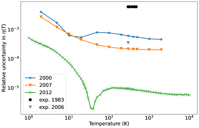
Figure 9: The evolution of the relative uncertainty in the ab initio calculation of viscosity for ⁴He. Stars: calculations from Ref. 4. Triangles: calculations from Ref. 5. Crosses: calculations from Ref. 6. The minimum of the calculated uncertainty near $40$ K is unphysical; see Sec. VI.3. Black dots: experimental data from Ref. 321. The gray triangle is the experimental value reported in Refs. 322, 323.

In the case of neon, the best theoretical estimates of transport coefficients are given in Ref. 112, while for argon they can be found in Ref. 159. In both cases, the best experimental results are obtained from ratio measurements using the ab initio value of the viscosity or thermal conductivity of helium.

V Molecular Systems

While the focus of this review is on noble gases, which are the fluids of choice for most ab initio-based primary temperature and pressure metrology, first-principles thermophysical properties for molecular species can also be of interest and make significant contributions. Three of the most promising areas are humidity metrology, low-pressure metrology, and atmospheric physics.

There are two main factors that make rigorous ab initio calculations of properties much more difficult for molecules than for monatomic species. The first is the increased dimensionality, where interactions depend not only on distance but on the relative orientations of the molecules. This not only complicates the development of potential-energy surfaces between molecules, but also makes the calculation of properties such as virial coefficients a sampling problem in many dimensions. Second, for rigorous calculations the internal degrees of freedom of the molecule must be considered, because properties of interest (such as the mean polarizability) depend on the molecular geometry and a distribution of geometries is sampled for each quantum state of the molecule. In some cases it may be adequate to assume a rigid molecule, but at a minimum an estimate of the uncertainty introduced by this assumption is needed, even though it might be difficult to compute.

In this section, we will describe the calculation of single-molecule quantities and quantities involving two or more molecules, along with the use of these quantities to calculate properties of interest for metrology. Particular attention will be given to methods for addressing the challenges specific to molecular species. Finally, we will discuss some metrological applications that use properties of molecular species.

V.1 Single-molecule calculations

V.1.1 Intramolecular potentials

In order to compute values of a property of a molecule averaged over nuclear motions, it is necessary to have a potential-energy surface for the molecule. Such surfaces can be developed with ab initio calculations, and they can often be refined if accurate spectroscopic measurements are available. Development of the intramolecular potential is relatively straightforward for diatomic molecules such as H₂, N₂, and CO because the potential is one-dimensional, but the dimensionality and complexity increases quickly with the number of atoms. Surfaces of sufficiently high quality for most purposes have been developed for the triatomic molecules H₂O [324] and CO₂. [325] These intramolecular potential-energy surfaces are also needed in order to sample configurations when considering molecular flexibility for pair calculations as described in Sec. V.2.2. Except for few-electron diatomics and two-electron triatomics, pure ab initio surfaces are not accurate enough to provide rovibrational spectra competitive with experiments, and the most accurate molecular surfaces are always semiempirical.

V.1.2 Electromagnetic properties

In contrast to noble gases, molecular species have multipole moments in the BO approximation (dipole, quadrupole, etc.). The most significant for metrology is the electric dipole moment. Rigorous ab initio calculation of the dipole moment for a molecule such as H₂O requires the development of a dipole-moment surface in which the dipole moment vector is given as a function of atomic coordinates, along with the single-molecule PES. The dipole moment for a given rovibrational state can then be computed as the expectation value averaged over the wave function of that state. Because the population of states changes with temperature, the average dipole moment will also change (slightly) with temperature; this has been analyzed for H₂O and its isotopologues by Garberoglio et al. [326]

The polarizability is another important quantity, both in the static limit for capacitance-based metrology and at higher frequencies for metrology based on optical refractivity. Unlike a noble gas whose polarizability at a given frequency is a single number, the polarizability of a molecule is a tensor that reflects the variation with directionality of the applied field and of the molecular axes. However, the quantity of interest for metrology is the mean polarizability, defined as $1/3$ of the trace of the polarizability tensor.

Polarizability reflects the response of the electrons to an electric field. It can be computed ab initio in a relatively straightforward way. While for monatomic species (and homonuclear diatomic species) the electronic polarizability is the only contribution, more complicated molecules have an additional contribution in the static limit and at low frequencies; this is usually called the vibrational polarizability. It can be thought of as the electric field distorting the molecule (and therefore its charge distribution) by pushing the negatively and positively charged parts of the molecule in opposite directions.

The molecular dipole moment and polarizability are defined as the first- and second-order response to an externally applied electric field $E_{0}$, respectively. They can be computed by numerical differentiation of the molecular energy computed in the BO approximation as a function of $E_{0}$, or by perturbation theory. Although in principle these two approaches should give the same result, in practice some differences are observed. For atomic systems, the results from perturbation theory are found to be more accurate than numerical differentiation and are generally preferred. [199] In the case of water, numerical differentiation is considered more accurate for dipole-moment calculations. [327]

Once intramolecular potential-energy surfaces, polarizability surfaces, and dipole-moment surfaces are available, one can calculate the temperature-dependent electromagnetic response of a molecule, that is the first dielectric virial coefficient $A_{\varepsilon}$ (see Eq. (8)), which is generally given by two contributions: [326] the first is proportional to the rovibrational and thermal average of the electronic polarizability surface, while the second depends on the squared modulus of the transition matrix element of the dipole-moment surface. Additionally, one can separate the contribution from the dipole-moment transition matrix elements into those transitions where the vibrational state of the molecule changes and those for which the vibrational state of the molecule does not change, but the rotational state does: these two components of the dipole-moment contribution to the molecular polarizability are known as vibrational and rotational polarizabilities, respectively. [328]

For small molecules (two or three atoms), one can solve directly the many-body Schrödinger equation for nuclear motion [329] (e.g., using the efficient discrete-variable representation [330] of the few-body Hamiltonian [331]) and then perform the appropriate rovibrational and thermal averages to obtain $A_{\varepsilon}$. It has recently been shown that the path-integral approach outlined in Sec. IV can be successfully used to compute the first dielectric virial coefficient of water. [326] It can possibly be generalized to larger molecules, where the direct solution of the many-body Schrödinger equation becomes very demanding in terms of computational power.

In the case of water, computational results using the most accurate intramolecular potential-energy surface, [324] polarizability surface, [332] and dipole-moment surface for water [327] are in good agreement with the experimental values of the dipole-moment contribution to $A_{\varepsilon}$ (which has an uncertainty of $\sim 5\%$), and within 0.1% of the experimental values for the static dipole moment, although the theoretical surfaces for water do not yet have rigorously assigned uncertainties.

V.1.3 Spectroscopy

It is now possible, especially for molecules containing only two or three atoms, to compute the positions and intensities of spectroscopic lines ab initio. The calculation of line positions requires only the single-molecule potential-energy surface. The more important quantity for thermodynamic metrology, however, is the intensity of specific lines. This requires both the PES and a surface for the dipole moment as a function of the coordinates. Accurate ab initio dipole-moment surfaces have been developed for H₂O, [327] CO₂, [333, 334] and CO. [335] The possible use in pressure metrology of intensities calculated from the surfaces for CO and CO₂ will be discussed in Sec. V.4

V.2 Calculations for molecular clusters

V.2.1 Interaction potentials

The development of interaction potentials for molecular gases is more difficult than for atomic ones due to the additional degrees of freedom, but much of the description in Sec. III is still applicable. A common approximation when developing intermolecular pair potentials is to treat the molecules as rigid rotors, which reduces the dimensionality considerably. For example, the PES of a pair of flexible water molecules has 12 degrees of freedom. By freezing the four OH bond lengths and the two HOH bond angles, only six degrees of freedom, usually taken to be the center-of-mass separation and five angles describing the mutual orientation, remain. To minimize the consequences of freezing the intramolecular degrees of freedom, the zero-point vibrationally averaged structures of the monomers are often used instead of the corresponding equilibrium structures. [336, 337]

However, even a six-dimensional dimer PES requires investigating thousands or even tens of thousands of pair configurations with high-level ab initio methods. As discussed in Sec. III, the most commonly applied level of theory is CCSD(T) [338] for molecular monomers; this method is usually applied with the frozen-core (FC) approximation. Such a level of theory was only the starting point in the schemes used to develop the most accurate pair potentials for the noble gases beyond helium. For the CCSD(T) method, the computational cost scales with the seventh power of the size of the molecules, and the scaling becomes even steeper for post-CCSD(T) methods.

In recent years, several intermolecular PESs have been developed that go beyond the CCSD(T)/FC level of electronic structure theory. The first step is to include all electrons in the calculations. Examples of all-electron (AE) surfaces are the flexible-monomer water dimer PES of Ref. 339 and the rigid-monomer ammonia dimer PES of Ref. 340. Also, post-CCSD(T)/AE terms were used in the H₂-CO flexible-monomer PESs starting in 2012. [341, 342] The T(Q) contributions were shown to have surprisingly large effects on the H₂-CO spectra. [343]

Intermolecular pair potentials can be accurately represented analytically by a number of different base functional forms. Mimicking the anisotropy of the PES is most commonly achieved either by using spherical harmonics expansions or by placing interaction sites at different positions in the molecules, with each site in one molecule interacting with each site in the other molecule through an isotropic function. The site-site potential form is also often used for the empirical effective pair potentials commonly employed in molecular dynamics and Monte Carlo simulations of large molecular systems. The analytical functions used to represent high-dimensional ab initio PESs for pairs of small rigid molecules typically have a few tens up to a few hundred fit parameters.

Determination of these parameters, i.e., fitting a PES to a set of grid points in a dimer configurational space and the corresponding interaction energies, was until recently a major task taking often several months of human effort. This bottleneck has recently been removed by computer codes that perform such fitting automatically. In particular, the autoPES program [344, 339] can develop both rigid- and flexible-monomer fits at arbitrary level of electronic structure theory. The automation is complete: a user just inputs specifications of monomers and the program provides on output an analytic PES. This means that the program determines the set of grid points, runs electronic structure calculations for each point, and performs the fit. In addition to developing automation, the autoPES project introduced several improvements in the strategy of generating PESs. In particular, the large-$R$ region of a PES is computed ab initio from the asymptotic expansion. Such expansion predicts interaction energies well down to $R$ about two times larger than the van der Waals minimum distance. This means that no electronic structure calculations are needed in this region and autoPES can develop accurate PESs for dimers of few-atomic monomers using only about 1000 grid points, while most published work used dozens of thousands of points.

Accurate analytical rigid-rotor PESs exist for a large number of both like-species and unlike-species molecule pairs. For metrology, the most noteworthy of these are the N₂–N₂, [345] CO₂–CO₂, [346, 347] H₂O–CO₂, [348] H₂O–N₂, [349] and H₂O–O₂. [350] Other accurate PESs of this type are: N₂–HF, [351] H₂O–H₂O, [352, 339] (HF)₂, [353] (HCl)₂, [354] CH₄–H₂O, [355, 356] and H₂–CO. [341, 343]

Many of these PESs (e.g., those from Refs. 345, 346, 348, 349, 350) are based on nonrelativistic interaction energies corresponding to the frozen-core CCSD(T) level of theory in the CBS limit and are represented analytically by site-site potential functions, with each individual site-site interaction being modeled by a modified Tang–Toennies type potential [357] with an added Coulomb interaction term. In the case of the N₂–N₂ PES, [345] corrections to the interaction energies for post-CCSD(T), relativistic, and core-core and core-valence correlation effects were considered. Motivated by the availability of extremely accurate experimental data for the second virial coefficients of N₂ and CO₂, the N₂–N₂ [345] and CO₂–CO₂ [346] PESs were additionally fine-tuned such that these data are almost perfectly matched by the values resulting from the PESs. The maximum well depths of the PESs were changed by the fine-tuning by less than 1%. Such fine-tuning does, however, mean that properties such as virial coefficients calculated from these tuned potentials cannot be considered to be truly from first principles for the purpose of metrology.

The second group of PESs listed above was also developed using either CCSD(T), with FC or AE, or SAPT. Post-CCSD(T) terms were considered in some cases, as already mentioned above. A range of different functional forms was used in the fitting, for larger monomers it was most often the site-site form.

While the error introduced by approximating molecules as rigid rotors is believed to be small for the molecules considered here, more rigorous calculations should include the intramolecular degrees of freedom; this has been done for example for the H₂–H₂, H₂–CO, and H₂O–H₂O potentials. [341, 342, 358, 359, 339] There are several difficulties involved in the generation of fully flexible potentials. The first one is the larger number of degrees of freedom. A system of $N$ molecules approximated as rigid rotors can be described by $C_{\mathrm{r}}=6N-6$ coordinates, while $C_{\mathrm{f}}=3nN-6$ coordinates are necessary to fully describe a configuration of the same molecules if each of the monomers has $n$ atoms. For sampling $c$ configurations per degree of freedom, the number of calculations needed to explore the potential-energy surface grows exponentially as $c^{C_{\mathrm{r|f}}}$. In the case of, say, the water trimer ($N=3$, $n=3$), even assuming $c=3$ one goes from $3^{12}\approx 5\times 10^{5}$ configurations for rigid models to $3^{21}\approx 10^{10}$ configurations for a fully flexible approach. The exponential increase of the number of configurations as a function of the number of degrees of freedom to be consdiered is sometimes called the dimensionality curse. Not all of these configurations are equally important and there is room for significant pruning and clever sampling strategies: one of the most useful starts from potentials developed for rigid molecules and enables the development of fully flexible versions optimizing the number of additional molecular configurations to be evaluated. [360, 361] More generally, even for a few degrees of freedom, the product of dimensions strategy leading to the $c^{C}$ is the worst strategy to follow. Instead, one uses various types of guided MC generation of grid points. In particular, the statistically guided grid generation method of Ref. 362 reduces the number of points needed for a 6-dimensional PES to about 300 (assuming the use of ab initio asymptotics). Another important issue regards the choice of a suitable form for the analytic potential and the fitting procedure. As in the case of rigid potentials, site-site interaction models (based on exponential functions at short range, inverse powers at long range, and Coulomb potentials) are commonly used also for intermolecular flexible potentials. For the intramolecular interactions, Morse functions are often used but polynomial expansions work sufficiently well for molecules in their low-energy rovibrational state. [339] Nevertheless, the dimensionality curse drastically limits the development of fully flexible potentials and for the time being only pair and three-body potentials involving diatomic and triatomic molecules (notably water [363, 364, 352]) have been developed.

V.2.2 Density virial coefficients

The calculation of density virial coefficients for molecular systems can be performed in a way very similar to that for noble gases. The main difference concerns the evaluation of the matrix elements of the free-molecule kinetic energy operator, that is the generalization of Eq. (63) which in turn depends on the specific degrees of freedom considered in the molecular model under consideration.

In the most general case, one considers the translational degrees of freedom of all the atoms in the molecule. Equation (63) remains the same (with the obvious modification of an atom-dependent mass $m$), but one needs an intramolecular potential to keep the molecule bound and, in general, a large number of beads, especially if light atoms (such as hydrogen or one of its isotopes) are to be considered. This approach allows flexibility effects to be fully accounted for and has been applied to investigate the second virial coefficient of hydrogen [358] and water [359] isotopologues. As one might expect, flexibility is more important at higher temperatures. On the other hand, this approach requires intramolecular and intermolecular potentials that depend on all the degrees of freedom, which in turn call for very demanding ab initio electronic structure calculations.

At sufficiently low temperatures, molecules occupy their vibrational ground state, and rigid monomer models are expected to be quite (although not perfectly) accurate. In this case, a whole molecule is described as a rigid rotor, that is by 3 translational and 3 rotational degrees of freedom (2 in the case of linear molecules). The matrix elements of the kinetic energy operator are, in this case, more complicated than that in Eq. (63), but their expression has been worked out for both linear [365] and non-linear [366, 367] rotors.

The rigid-rotor approximation of a molecular system is, in principle, an uncontrolled approximation and, consequently, cannot directly provide useful data for metrological applications. On the other hand, the associated uncertainties can be partially offset by the fact that potential-energy surfaces can be generated higher accuracy than in the case of fully flexible models. [254, 368] Validation of the ab initio results with experimental data can be used to establish the temperature range in which a rigid model is valid, and provide useful estimates of virial coefficients where experimental data are lacking. Additionally, rigid models can be a stepping stone towards the more accurate fully flexible approaches.

Also, semiclassical approximations of density [369] or dielectric virial coefficients [276] for molecular systems are available. They are generally much easier to evaluate than by path-integral calculations, and are quite accurate in many cases. [359, 326]

V.2.3 Dielectric and refractivity virial coefficients

The calculation of dielectric and refractivity virial coefficients for molecular species is much more difficult than for the monatomic systems discussed in Sec. IV.5.3. In addition to the increased dimensionality, the charge asymmetry creates additional polarization effects in interacting molecules. A complete treatment must therefore include the effect of the molecular interactions not only on the polarizability of the molecules, but also on their charge distribution. Because of this complexity, it seems unlikely that coefficients beyond the second virial will be calculated in the foreseeable future, and quantitatively accurate calculations with realistic uncertainty estimates may be limited to diatomic molecules such as N₂ or H₂.

The only attempt at such calculations we are aware of for realistic (polarizable) molecular models is the work of Stone et al., [370] who calculated the second dielectric virial coefficient for several small molecules, including CO and H₂O. A recent experimental determination of the second dielectric virial coefficient for CO [371] was in qualitative but not quantitative agreement with the prediction of Stone et al.

For rigorous metrology, it would be necessary to characterize the uncertainty of the surfaces describing the mutual polarization and pair polarizability of the molecules. The dimensionality, and therefore the complexity, of these calculations for a diatomic molecule like N₂ would be similar to that for the three-body polarizability and dipole surfaces for monatomic gases.

V.2.4 Molecular collisions

In some pressure-metrology applications near vacuum conditions, collision rates, which are related to collision integrals, are required. We already introduced collision integrals for atom-atom collisions in Sec. IV.6, but the concept can be generalized to include atom-molecule and molecule-molecule collisions, which enables the calculation of transport properties for dilute molecular gases. While the collision integrals for atom-atom collisions result in a classical treatment from the solution of the linearized Boltzmann equation and in the quantum-mechanical case from the solution of the linearized Uehling–Uhlenbeck equation, [372] the corresponding classical and quantum-mechanical equations for collisions involving molecules are the linearized Curtiss–Kagan–Maksimov equation [373, 374, 375, 376] and the linearized Waldmann–Snider equation. [377, 378, 379, 380]

The formalism for the calculation of collision integrals involving molecules is much more complex than in the case of atom-atom collisions. Relations for classical collision integrals were derived by Curtiss for rigid linear molecules [381] and extended to rigid nonlinear molecules by Dickinson et al. [382] The quantum-mechanical calculation of collision integrals involving two molecules has rarely been attempted because of the mathematical complexity and large computational requirements, whereas atom-molecule collisions have been studied quantum-mechanically more often. For collisions between a helium atom and a nitrogen molecule, collision integrals were calculated both classically and quantum-mechanically. [383, 384] The comparison showed that quantum effects are small except at low temperatures. The degree to which the quantum nature of collisions can be neglected for pairs with larger expected quantum effects, such as H₂O–H₂O, remains an open question, but the agreement with experiment of classically calculated dilute-gas viscosities for H₂O [385] suggests that the classical approximation is adequate for most purposes.

V.3 Humidity metrology

Much humidity metrology requires knowledge of humid air’s departure from ideal-gas behavior. Because the densities are low, this can be described by the virial expansion. The second virial coefficient of pure water has been calculated [359] based on flexible ab initio pair potentials computed at a high level of theory. [363, 364, 352] It is necessary to take the flexibility of the water molecule into account to obtain quantitative accuracy. [359]

The most important contribution to the nonideality of humid air comes from the interaction second virial coefficient of water with air. While fairly accurate measurements of this quantity exist near ambient temperatures, it can now be computed with similar or better uncertainty by combining the cross second virial coefficients for water with the main components of dry air. [386] Good quality pair potentials exist for water with argon, [387] nitrogen, [349] and oxygen, [350] and these have been combined by Hellmann [350] to produce accurate water-air second virial coefficients between 150 K and 2000 K.

For humidity metrology at pressures significantly higher than atmospheric, corrections at the third virial coefficient level become significant. Only very limited data exist for the relevant third virial coefficients (water-water-air and water-air-air), [388] so ab initio calculation of these quantities would be useful. This requires development of three-body potential-energy surfaces for systems such as H₂O–N₂–N₂ and H₂O–H₂O–O₂. To our knowledge, no high-accuracy surfaces exist for these three-molecule systems, but their development should be feasible with current technology.

The same framework can be used for humidity metrology in other gases. Hygrometers are typically calibrated with air or nitrogen as the carrier gas, but some error will be introduced if the calibration is used in the measurement of moisture in a different gas. Calibrations can be adjusted if ab initio values of the cross second virial coefficient are known for water with the gas of interest. Such values have been developed for several important gases, such as carbon dioxide, [348] methane, [389] helium, [390] and hydrogen. [391]

Some emerging technologies for humidity metrology can be aided by ab initio property calculations. Instruments to measure humidity from the change in dielectric constant with water content of a gas [392, 393] require the first dielectric virial coefficient of water, which depends on its molecular polarizability and dipole moment. These quantities, and their temperature dependence, have been a subject of recent theoretical study. [326]

Spectroscopic measurement of humidity has also been proposed; [394] this requires the intensity of an absorption line for the water molecule. Thus far, work in this area has used measured line intensities due to their smaller uncertainty compared to ab initio values. The recent work of Rubin et al. [395] demonstrated mutually consistent sub-percent accuracy for both experimental and theoretical intensities based on a semiempirical PES for an H₂O line, offering promise for the future use of calculated intensities to reduce the uncertainty of humidity metrology.

V.4 Pressure metrology

Molecular calculations are also promising for pressure metrology at low pressures. [99] Refractivity-based pressure measurements using noble gases are discussed in Sec. II.3. Some proposed approaches use ratios of the refractivity of a more refractive gas (such as nitrogen or argon) to that of helium. Use of nitrogen in these systems would be aided by good ab initio results for the polarizability of the N₂ molecule and its second density and refractivity virial coefficients.

For low pressures, on the order of 1 Pa and below, absorption spectroscopy is a promising approach for pressure measurement. The absorption of a gas such as CO or CO₂ can be used to measure low gas densities (from which the pressure is calculated by the ideal-gas law, perhaps with a second virial correction); this can be a primary pressure standard if the line intensity is calculated from semiempirical potential-energy and dipole-moment ab initio surfaces tuned to spectral data. Even if measured intensities are used, theoretical results are valuable to check their accuracy. For CO₂, uncertainty of intensity measurements and agreement between theory and experiment below 0.5% has been obtained. [334, 396] The simpler CO molecule is more amenable to accurate theoretical calculations; consistency between experimental and theoretical line intensities on the order of 0.1% has recently been achieved. [335] In these calculations, the potential energy curve was purely empirical, but the dipole-moment surface was obtained ab initio. An unresolved question in this work so far is the uncertainty of ab initio calculated line intensities, which must depend in a complex way on the uncertainties in the intramolecular potential and in the dipole-moment surface. Without reasonable estimates for the uncertainty of calculated intensities, the utility of this spectroscopic method for primary pressure standards is diminished.

For ultrahigh vacuum and below, gas densities can be measured based on the collision rate between the gas and a collection of trapped ultra-cold atoms. Both lithium and rubidium have been proposed as the trapped species. [397, 398, 399, 400, 401, 402, 403] While in some implementations an apparatus constant is derived from measurements, [399, 400] it has recently been recognized [404] that the proposed procedure introduces error when light species (such as Li and H₂) are involved in the collisions.

It is also possible to determine the relevant proportionality factor for the collision rate from first principles using collision cross sections calculated from ab initio pair potentials and quantum collision theory. These calculations have been performed for lithium with H₂ (the most common gas in metallic vacuum systems) and He; [405, 406] ab initio calculations with rubidium are more challenging due to the large number of electrons. A recent paper has reported first-principles collision rate coefficients for both Rb and Li with noble gases, H₂, and N₂. [407] It is also possible to measure the ratio of two collision pairs (for example, Rb–H₂ versus Li–H₂) to obtain the coefficient for a system that is more difficult to calculate ab initio; [397, 404] in this approach a low uncertainty for the simpler-to-calculate system (that with fewer electrons) is essential.

V.5 Atmospheric physics

In atmospheric physics, the interaction of radiation with atmospheric gases, particularly H₂O and CO₂, has received increasing attention for climate studies; it is also important for Earth-based astronomy where the atmosphere is in the optical path. Scientists in these fields rely on line positions and intensities in the HITRAN database. [408] Increasingly, ab initio calculations are being used to supplement experimental measurements for these quantities, as has recently been summarized for CO₂. [409]

V.6 Transport properties

While transport properties of molecular gases are of little relevance in precision metrology, for the sake of completeness we mention briefly the current state of the art for pure molecular gases. Most of the transport property calculations for such gases performed so far are based on classically calculated collision integrals for rigid molecules using the formalism of Curtiss [373] for linear molecules and of Dickinson et al. [382] for nonlinear molecules (see Sec. V.2.4.)

A representative example of such calculations for gases consisting of small molecules other than H₂ are the classical shear viscosity and thermal conductivity calculations of Hellmann and Vogel [385] and Hellmann and Bich, [410] respectively, for pure H₂O. The agreement with the best experimental data is within a few tenths of a percent for the viscosity and a few percent for the thermal conductivity. For both properties, these deviations correspond to the typical uncertainties of the best experimental data. The significant contribution to the thermal conductivity due to the transport of energy “stored” in the vibrational degrees of freedom, which is not directly accounted for by the classical rigid-rotor calculations, was estimated using a scheme that only requires knowledge of the ideal-gas heat capacity in addition to the rigid-rotor collision integrals. [410] The main assumption in this scheme is that collisions that change the vibrational energy levels of the molecules are so rare that their effects on the collision integrals are negligible.

For pure H₂, classical calculations are not accurate enough even at ambient temperature. Fully quantum-mechanical calculations were performed by Mehl et al. [411] using a spherically-averaged modification of a H₂–H₂ PES, [254] thus reducing the complexity of the collision calculations to that for monatomic gases. Despite this approximation, the calculated shear viscosity and thermal conductivity values for H₂ agree very well with the best experimental data, particularly in the case of the viscosity where the agreement is within 0.1%.

VI Concluding Remarks and Future Perspectives

The outstanding progress achieved during the last three decades by the ab initio calculation of the thermophysical properties of pure fluids and mixtures has drastically reduced the uncertainty of the measurement of these properties and of the thermodynamic variables temperature, pressure, and composition.

For example, consider primary thermometry. Ab initio calculations directly contributed to the acoustic and dielectric determination of the value of the Boltzmann constant that is used in the new SI definition of the kelvin. The remarkably accurate theoretical calculations of the polarizability and the non-ideality of thermometric gases have also facilitated simplified measurement strategies and techniques. [24, 48, 49] Consequently, new paths directly disseminating the thermodynamic temperature are now available at temperatures below $25$ K, where the realization of ITS-90 is particularly complicated. Various methods of gas thermometry have determined $T$ with uncertainties that are comparable to or even lower than the uncertainty of realizations of ITS-90. [30, 57, 58] Improved theory has also suggested that primary CVGT could usefully be revisited, as discussed in Section II.2.4.

In the near future, technical achievements will likely further reduce the uncertainty of measurements of the thermodynamic temperature and the thermophysical properties of gases. Efforts are underway to improve: (1) the purity of the thermometric gases at their point of use, (2) implementing two-gas methods to reduce the uncertainties from compressibility of the apparatus, and (3) developing robust microphones (possibly based on optical interferometry) to facilitate cryogenic AGT. In the remainder of this section, we will summarize current limitations and describe some prospects for future contributions.

VI.1 Current limitations of ab initio property calculations

As described in Sec. III, ab initio calculations of properties for individual helium atoms and pairs of atoms have achieved extraordinarily small uncertainties. Even for three-body interactions, the potential energy is now known with small uncertainty, and good surfaces are available for the three-body polarizability and dipole moment surfaces. This enables accurate calculations, with no uncontrolled approximations, of the second and third density, acoustic, and dielectric virial coefficients. This high level of accuracy is due to the small number of electrons involved; electron correlation at the FCI level is still tractable for three helium atoms with a total of six electrons.

For DCGT and RIGT, it would be desirable to have similarly accurate properties for neon and argon, because their higher polarizability (and therefore stronger response) reduces the relative effect of other sources of uncertainty such as imperfect knowledge of the compressibility of the apparatus or the presence of impurities in the gas. Unfortunately, this level of accuracy for neon and argon is unlikely to be obtained in the foreseeable future. The neon atom has 10 electrons, as many as five helium atoms, and argon has 18. While recent efforts have (at large computational expense) significantly reduced the uncertainty of single-atom and dimer quantities for neon and argon, [59, 60, 61, 112, 113] they do not approach the levels of accuracy achieved for helium. For example, the relative uncertainty of the best calculation of the static polarizability of a neon atom [60] is more than $100$ times greater than that of a helium atom. [187] Similarly, the relative uncertainty of the pair potential minimum energy is about $100$ times larger for neon [112] than for helium. [7] Therefore, the relative uncertainties of calculated gas-phase thermophysical properties will be much higher for other gases than for helium. In such cases, the most accurate values of properties will be obtained by measuring ratios of properties relative to that of helium. This has already been done for the static polarizability of neon and argon [58] and for the low-density viscosity of several gases. [161, 162, 163]

Refractivity-based thermal metrology [76, 312] requires $A_{\mathrm{R}}$, and preferably also $B_{\mathrm{R}}$ and $C_{\mathrm{R}}$. At microwave frequencies, the static values ($A_{\varepsilon}$, $B_{\varepsilon}$, etc.) can be used. At optical frequencies, $A_{\mathrm{R}}$ and $B_{\mathrm{R}}$ have been computed at a state-of-the-art level for helium, [73, 78] but corresponding calculations for neon and argon rely on values for the dynamic polarizability and for the Cauchy moment $\Delta S(-4)$ that could be significantly improved. Even with state-of-the-art ab initio results, it seems likely that ratio measurements using helium, such as those of Egan et al. for $A_{\mathrm{R}}$, [114] will produce lower uncertainties. To our knowledge, the theory for calculating $C_{\mathrm{R}}$ at optical frequencies is not available. Therefore, at the moment, it is necessary to take rather uncertain values from experiment or assume (based on the small difference between $B_{\mathrm{R}}$ and $B_{\varepsilon}$) that it is equal to $C_{\varepsilon}$.

As mentioned in Sec. IV.5.3 and also noted by Rourke, [312] another issue for refractivity methods is the unclear situation surrounding the $A_{\mu}$ contribution. The best calculations of the magnetic susceptibility for helium, [74] neon, [59] and argon [61] disagree with the old, sparse measurements of these quantities [316] by amounts much larger than their stated uncertainties. Independent calculations of the magnetic susceptibility for one or more of these species would be helpful in assessing this discrepancy, but what is most needed is a modern measurement of the magnetic susceptibility of a noble gas (probably argon), either as an absolute measurement or as a ratio to a substance with a better-known magnetic susceptibility, such as liquid water.

To reach higher pressures with helium-based apparatus, it would be desirable to have reliable values, with uncertainties, for the fourth virial coefficient $D(T)$. The most complete first-principles estimate so far [122] used high-accuracy two-body and three-body potentials, but had a significant uncertainty component due to the unknown four-body potential. Accurate calculations of the nonadditive four-body potential for helium are feasible with modern methods.A four-body PES for helium, even if its relative uncertainty was as large as 10%, would allow reference-quality calculation of $D(T)$ and enable improved metrology.

VI.2 Molecular gases

Nitrogen is an attractive option for gas-based metrology due to its availability in high purity and its longstanding use in traditional apparatus such as piston gauges, but its lack of spherical symmetry and its internal degree of freedom add complication to ab initio calculation of its properties. The development of potential-energy surfaces for pair and three-body interactions for rigid molecular molecules is certainly feasible. This is also possible for flexible models, pending the difficulties already discussed in Sec. V.2.1. Once this data is available, the methods for calculations of density virial coefficients have already been proven. [254, 368, 359] (see Sec. V.2.2.) To the best of our knowledge, no fully ab initio calculation of dielectric virial coefficients for molecular systems has been performed. This task will require the development of the molecular interaction-induced polarizability function. The path-integral approach described in Sec. IV can certainly be extended to compute these quantities as well as rigorously propagate their uncertainties.

VI.3 Improved uncertainty estimations

As mentioned in Sec. IV.3, much progress has been made in estimating realistic uncertainties for density and dielectric virial coefficients. The old method of simply displacing the potentials in a “plus” and “minus” direction, while correct for one-dimensional integrations such as $B$ and $B_{\varepsilon}$, is inefficient and can produce inaccurate results for higher coefficients. The functional differentiation approach discussed in Sec. IV.3 provides more rigorous results.

However, it is not entirely clear how to obtain uncertainties for acoustic virial coefficients, because they involve temperature derivatives of $B(T)$ and $C(T)$. The rigorous assignment of uncertainty to a derivative of a function computed from uncertain input is an unsolved problem as far as we are aware. Binosi et al. [292] recently applied a statistical method (the Schlessinger Point Method) to the estimation of uncertainties for acoustic virial coefficients; this may provide a way forward.

A similar issue exists for the low-density transport properties. The very low uncertainty of the viscosity of helium shown in Fig. 9 near $40$ K, obtained with the traditional method of “plus” and “minus” perturbations to the pair potential, is an artifact of competing effects on the collision integral of perturbations from different parts of the potential. While $B(T)$, for example, exhibits monotonic behavior with respect to perturbations in the potential, that is not the case for the collision integrals used to compute transport properties, which can cause uncertainties to be artificially underestimated. This was recognized by Hellmann and coworkers, who created potentials perturbed in additional ways to provide a non-rigorous but reasonable estimation method for the uncertainty of low-density transport properties for krypton, [144] xenon, [412] and neon. [112] Further analysis would be welcome to improve the rigor of uncertainty estimates for transport collision integrals.

VI.4 Transport properties

In addition to the uncertainty issue just mentioned, we see two areas for improvement in the field of transport properties. The first concerns the density dependence beyond the low-density limiting values discussed in this work. As mentioned in Sec. II.5, for flow metrology it would be desirable to know the viscosity with small and rigorous uncertainties not only at zero density, but at the real densities at which instruments are calibrated. The first correction should be a virial-like term linear in density, but the most successful theory so far [166, 167, 168] relies on some simplifying assumptions. A more rigorous theory would be a significant advance. Even if the initial density dependence were only known for helium, that would enable better metrology for other gases because of the established methods for measuring viscosity ratios.

The second area is the transport properties of molecular species, such as N₂ or H₂O. As mentioned in Sec. IV.6, classical collision integrals can be calculated for these species when they are modeled as rigid rotors. While it is believed that the errors introduced by the assumptions of classical dynamics and rigid molecules are small, it would be desirable to have verification from a more rigorous calculation. One might expect quantum effects to be significant for the dynamics of H₂O collisions, since they make a large contribution to $B(T)$ for H₂O. [358] Since fully quantum calculation of collision integrals is currently intractable for all but the simplest systems, the development of a viable “semiclassical” method for transport properties would be desirable. No such formulation exists to our knowledge.

VI.5 Simulations of liquid helium

While we have focused on the gaseous systems where ab initio properties are already making major contributions to metrology, the thermophysical properties of condensed phases (particularly for helium) are also important in temperature metrology. For example, the vapor pressures of liquid ³He and ⁴He are part of the definition of ITS-90. [413] With highly accurate two- and three-body potentials for helium (perhaps eventually supplemented by a four-body potential), high-accuracy simulation of thermodynamic properties of liquid helium may become feasible.

In fact, path-integral simulations of liquid ⁴He can be performed without uncontrolled approximations, [272] although, to the best of our knowledge, the most recent ab initio potentials have not been employed yet to compute any liquid helium property (e.g., the specific heat – and hence the vapor pressure, via the Clapeyron equation – or the temperature of superfluid transition). Consequently, the accuracy of first-principles many-body potentials in the case of fluid phases of ⁴He is largely unknown. The use of three-body (or higher, when available) potentials is expected to require considerable computational resources, as has been recently observed in simulations of liquid para-H₂, [414] but theoretical developments in efficient simulation methods for degenerate systems [415] might pave the way for a fully ab initio calculation of the thermophysical properties of condensed ⁴He.

In the case of fermionic systems such as ³He, the path-integral approach suffers in principle from a “sign problem” [416] which generally requires some approximations, and results in a large statistical uncertainty. However, two research groups have recently claimed to have overcome these limitations, [417, 418] which might result in accurate calculations of thermophysical properties in the liquid phase also for this isotope.

VI.6 Reproducibility and validation

It is desirable for metrological standards to be based on multiple independent studies, so that they will not be distorted by a single unrecognized error. For example, for the recent redefinition of the SI in which several fundamental physical constants were assigned exact values, it was required that the value assigned to the Boltzmann constant be based on consistent results from at least two independent experiments using different techniques and meeting a low uncertainty threshold. [23] Similarly, metrological application of the calculated results discussed in this Review would be on a firmer basis if there was independent confirmation of the results.

The danger of an unrecognized error in calculated quantities is not merely hypothetical. For several years, the “best” calculated values of $C$ for ³He were in error below about 4.5 K because the effects of nuclear spin on the quantum exchange contribution had been incorporated incorrectly; this was eventually recognized and corrected in Errata. [123, 122] An early quantum calculation of $B_{\varepsilon}$ of argon [419] disagreed with a later study, [73] apparently because of inexact handling of resonance states in the earlier work. Ideally, there would be independent confirmation of all the results cited in Table 4 so that any errors could be detected.

One helpful step in this direction would be more complete documentation of calculations, including computer code, so that others can reproduce or check the work. It is common to provide computer code for potential-energy surfaces, but the calculation of virial coefficients has typically been performed with specialized software that is not public.

More important for metrology, however, would be independent verification of the calculated results. Conceptually, this has two parts: validation of the calculated quantities and surfaces described in Sec. III (potential-energy, polarizability, and dipole surfaces; atomic and magnetic polarizabilities) and validation of the calculation of virial coefficients from these quantities (described in Sec. IV).

Validation of calculated virial coefficients is probably the easier of the two parts, because it is typically less computationally demanding. This has been done for a few quantities; for example, two groups have performed fully quantum calculations (in one case neglecting exchange effects that become important below 7 K) of $C$ [123, 308] and $D$ [308, 122] for ⁴He. Consistency checks can also be made by comparing different calculation methods, including classical and semiclassical approaches that should agree with the quantum calculations at high temperatures. The error in $B_{\varepsilon}$ for argon mentioned above was detected by comparing phase-shift calculations to PIMC and semiclassical calculations, showing the value of multi-method comparisons.

The independent validation of calculated atomic quantities and intermolecular surfaces is more difficult, because these require large amounts of dedicated computer time. There have been a few cases where parallel efforts have produced independent, high-quality results; these include $A_{\varepsilon}$ for neon [59, 60] and the three-body potential of argon. [118, 268] Some validation is also provided when the state of the art advances and new potentials are produced that agree with previous potentials (but have smaller uncertainties); this has been the case with the sequential development of pair potentials for helium (Sec. III.3). In some cases, however, these are not truly independent verifications because they are developed by the same group and use many of the same methods. While it may be difficult to justify the extensive work required to independently confirm a state-of-the-art calculated surface, there would be value in performing spot checks of a few points. This would require developers of surfaces to make their calculated points available (or at least a subset of them), and also the multiple calculated quantities that typically contribute to each point.

We believe that more attention should be paid to the reproducibility and validation of the calculated results that are increasingly important in precision metrology. Work of this nature may not be very attractive to funding agencies (or graduate students), but it is needed for more confident use of gas-based metrology.

Author Declarations

Conflict of Interest

The authors have no conflicts to disclose.

Appendix A Formulae for the Third Acoustic Virial Coefficient, $\gamma_{\mathrm{a}}$

As is apparent from Eqs. (35), (36), and (32), the explicit expression of the third acoustic virial coefficient as a function of the pair and three-body potential is quite involved. We found that it is most conveniently expressed by defining

$$b(r,T) = U_{2}(r)\mathrm{e}^{-\beta U_{2}(r)}-1$$ (95)

$$b_{T}(r,T) = \beta U_{2}(r)\mathrm{e}^{-\beta U_{2}(r)}$$ (96)

$$b_{TT}(r,T) = \beta U_{2}(r)(\beta U_{2}(r)-2)\mathrm{e}^{-\beta U_{2}(r)}$$ (97)

and

$$c = \mathrm{e}^{-\beta U_{3}}-\sum_{i<j}\mathrm{e}^{-\beta U_{2}(r_{ij})}+2$$ (98)

$$c_{T} = \beta U_{3}\mathrm{e}^{-\beta U_{3}}-\sum_{i<j}\beta U_{2}(r_{ij})\mathrm{e}^{-\beta U_{2}(r_{ij})}$$ (99)

$$c_{TT} = \beta U_{3}(\beta U_{3}-2)\mathrm{e}^{-\beta U_{3}}-$$ (100)

$$\sum_{i<j}\beta U_{3}(\beta U_{3}-2)\mathrm{e}^{-\beta U_{3}},$$

where $c$, $c_{T}$ and $c_{TT}$ are functions of the temperature $T$ as well as $r_{12}$,$r_{13}$, and $r_{23}$ through their dependence on $U_{3}$. Performing the substitution $\gamma_{0}=5/3$, we obtain

$$RT\gamma_{\mathrm{a}}(T) = \frac{8\pi^{3}}{3}N_{\mathrm{A}}^{2}\int\left[\frac{2}{15}b_{TT}(r_{12})b_{TT}(r_{13})+\frac{14}{15}b_{T}(r_{12})b_{TT}(r_{13})+b(r_{12})b_{TT}(r_{13})+\right.$$ (101)

$$\frac{73}{30}b_{T}(r_{12})b_{T}(r_{13})+\frac{34}{5}b(r_{12})b_{T}(r_{13})+\frac{33}{5}b(r_{12})b(r_{13})-$$

$$\left.\left(\frac{2}{15}c_{TT}(r_{12},r_{13},r_{23})+\frac{16}{15}c_{T}(r_{12},r_{13},r_{23})+\frac{13}{5}c(r_{12},r_{13},r_{23})\right)\right]\mathrm{d}\Omega_{3}.$$

The path-integral expression for $\gamma_{\mathrm{a}}$ is more complicated, due to the fact that the ring-polymer distribution function $F$ of Eq. (66) depends on temperature. In particular, defining $\cal U$ so that

$$F=\Lambda^{3}\left(\frac{P^{3/2}}{\Lambda^{3}}\right)^{P}\exp\left(-\beta{\cal U}\right),$$ (102)

one can show that

$$\frac{\mathrm{d}F}{\mathrm{d}\beta}=\left({\cal U}-\frac{3(P-1)}{2\beta}\right)F,$$ (103)

and derive path-integral expressions for $\gamma_{\mathrm{a}}$. However, this straightforward approach is characterized by large variance in the Monte Carlo simulations, since Eq. (103) has a form analogous to the thermodynamic estimator of the kinetic energy. [290] It is possible to derive equivalent expressions with smaller variance, using the same ideas that lead to the virial estimator. [420, 290] The resulting formulae are very cumbersome, and can be found in Ref. 292.

References

- McEvoy et al. [2020] H. C. McEvoy et al., “Methodologies and uncertainty estimates for measurements over the temperature range from 430 K to 1358 K under the auspices of the EMPIR InK2 project,” Meas. Sci. Technol. 32, 035001 (2020).
- Rowlinson [1973] J. S. Rowlinson, “Legacy of van der Waals,” Nature 244, 414 (1973).
- Aziz, Janzen, and Moldover [1995] R. A. Aziz, A. R. Janzen, and M. R. Moldover, “Ab initio calculations for helium: a standard for transport property measurements,” Phys. Rev. Lett. 74, 1586 (1995).
- Hurly and Moldover [2000] J. J. Hurly and M. R. Moldover, “Ab initio values of the thermophysical properties of helium as standards,” J. Res. Natl. Inst. Stand. Technol. 105, 667 (2000).
- Hurly and Mehl [2007] J. J. Hurly and J. B. Mehl, “4He thermophysical properties: New ab initio calculations,” J. Res. Natl. Inst. Stand. Technol. 112, 75 (2007).
- Cencek et al. [2012] W. Cencek, M. Przybytek, J. Komasa, J. B. Mehl, B. Jeziorski, and K. Szalewicz, “Effects of adiabatic, relativistic, and quantum electrodynamics interactions on the pair potential and thermophysical properties of helium,” J. Chem. Phys. 136, 224303 (2012).
- Czachorowski et al. [2020] P. Czachorowski, M. Przybytek, M. Lesiuk, M. Puchalski, and B. Jeziorski, “Second virial coefficients for 4He and 3He from an accurate relativistic interaction potential,” Phys. Rev. A 102, 042810 (2020).
- White et al. [1960] D. White, T. Rubin, P. Camky, and H. L. Johnston, “The virial coefficients of helium from to K,” J. Phys. Chem. 64, 1607 (1960).
- Berry [1979] K. Berry, “NPL-75: A low temperature gas thermometry scale from K to K,” Metrologia 15, 89 (1979).
- Kemp, Kemp, and Besley [1986] R. Kemp, W. Kemp, and L. Besley, “A determination of thermodynamic temperatures and measurements of the second virial coefficient of 4He between K and K using a constant-volume gas thermometer,” Metrologia 23, 61 (1986).
- Gaiser and Fellmuth [2009] C. Gaiser and B. Fellmuth, “Helium virial coefficients—a comparison between new highly accurate theoretical and experimental data,” Metrologia 46, 525 (2009).
- Gaiser and Fellmuth [2021a] C. Gaiser and B. Fellmuth, “Highly-accurate second-virial-coefficient values for helium from 3.7 K to 273 K determined by dielectric-constant gas thermometry,” Metrologia 58, 015013 (2021a).
- Madonna Ripa et al. [2021] D. Madonna Ripa, D. Imbraguglio, C. Gaiser, P. Steur, D. Giraudi, M. Fogliati, M. Bertinetti, G. Lopardo, R. Dematteis, and R. M. Gavioso, “Refractive index gas thermometry between K and K,” Metrologia 58, 025008 (2021).
- Egan et al. [2016] P. F. Egan, J. A. Stone, J. E. Ricker, and J. H. Hendricks, “Comparison measurements of low-pressure between a laser refractometer and ultrasonic manometer,” Rev. Sci. Instrum. 87, 053113 (2016).
- Gaiser, Fellmuth, and Sabuga [2020] C. Gaiser, B. Fellmuth, and W. Sabuga, “Primary gas-pressure standard from electrical measurements and thermophysical ab initio calculations,” Nature Phys. 16, 177 (2020).
- Gaiser et al. [2022] C. Gaiser et al., “2022 Update for the differences between thermodynamic temperature and ITS-90 below K,” J. Phys. Chem. Ref. Data 51, 043105 (2022).
- White and Fischer [2015] D. R. White and J. Fischer, “The Boltzmann constant and the new kelvin,” Metrologia 52, S213 (2015).
- Fischer et al. [2011] J. Fischer et al., “Present estimates of the differences between thermodynamic temperatures and the ITS-90,” Int. J. Thermophys. 32, 12 (2011).
- Cohen and Taylor [1973] E. R. Cohen and B. N. Taylor, “The 1973 least-squares adjustment of the fundamental constants,” J. Phys. Chem. Ref. Data 2, 663 (1973).
- Newell et al. [2018] D. B. Newell et al., “The CODATA 2017 values of , , , and for the revision of the SI,” Metrologia 55, L13 (2018).
- Pitre et al. [2017] L. Pitre et al., “New measurement of the Boltzmann constant by acoustic thermometry of helium-4 gas,” Metrologia 54, 856 (2017).
- de Podesta et al. [2017] M. de Podesta et al., “Re-estimation of argon isotope ratios leading to a revised estimate of the Boltzmann constant,” Metrologia 54, 683 (2017).
- Fischer et al. [2018] J. Fischer et al., “The Boltzmann project,” Metrologia 55, R1 (2018).
- Moldover et al. [2014] M. R. Moldover, R. M. Gavioso, J. B. Mehl, L. Pitre, M. de Podesta, and J. T. Zhang, “Acoustic gas thermometry,” Metrologia 51, R1 (2014).
- Note [1] Notice that in the literature one might find multiple and inconsistent definitions of the acoustic virial coefficients, depending on the variable chosen for the expansion of (the pressure or the molar density ) and the powers of included in the definition of the acoustic virials. We used the convention put forward in Ref. \rev@citealpnumGillis1996; in this case has the same dimensions as the second virial coefficient and has the same dimensions as the third virial coefficient .
- Moldover et al. [1999] M. R. Moldover, S. J. Boyes, C. W. Meyer, and A. R. Goodwin, “Thermodynamic temperatures of the triple points of mercury and gallium and in the interval K to K,” J. Res. Natl. Inst. Stand. Technol. 104, 11 (1999).
- Morantz [2017] P. Morantz, Ph.D. thesis, Cranfield University (2017).
- Mehl and Moldover [1986] J. B. Mehl and M. R. Moldover, “Measurement of the ratio of the speed of sound to the speed of light,” Phys. Rev. A 34, 3341 (1986).
- Underwood et al. [2010] R. Underwood, D. Flack, P. Morantz, G. Sutton, P. Shore, and M. de Podesta, “Dimensional characterization of a quasispherical resonator by microwave and coordinate measurement techniques,” Metrologia 48, 1 (2010).
- Mehl [2009] J. B. Mehl, “Second-order electromagnetic eigenfrequencies of a triaxial ellipsoid,” Metrologia 46, 554 (2009).
- Yang, Underwood, and de Podesta [2018] I. Yang, R. Underwood, and M. de Podesta, “Investigating the adequacy of a low-cost vector network analyser for microwave measurements in quasispherical resonators,” Meas. Sci. Technol. 29, 075013 (2018).
- Corbellini and Gavioso [2013] S. Corbellini and R. M. Gavioso, “A low-cost instrument for the accurate measurement of resonances in microwave cavities,” IEEE Trans Instrum Meas 62, 1259 (2013).
- Zhang et al. [2016] K. Zhang, X. J. Feng, J. T. Zhang, H. Lin, Y. N. Duan, and Y. Y. Duan, “Microwave measurements of the length and thermal expansion of a cylindrical resonator for primary acoustic gas thermometry,” Meas. Sci. Technol. 28, 015006 (2016).
- Strouse et al. [2003] G. F. Strouse, D. R. Defibaugh, M. R. Moldover, and D. C. Ripple, “Progress in primary acoustic thermometry at NIST: 273 K to 505 K,” AIP Conference Proceedings, 684, 31 (2003).
- Yang et al. [2015] I. Yang, L. Pitre, M. R. Moldover, J. Zhang, X. Feng, and J. S. Kim, “Improving acoustic determinations of the Boltzmann constant with mass spectrometer measurements of the molar mass of argon,” Metrologia 52, S394 (2015).
- Moldover, Mehl, and Greenspan [1986] M. R. Moldover, J. B. Mehl, and M. Greenspan, “Gas-filled spherical resonators: Theory and experiment,” J. Acoust. Soc. Am. 79, 253 (1986).
- Gillis [2012] K. A. Gillis, “Second-order boundary corrections to the radial acoustic eigenvalues for a spherical cavity,” Metrologia 49, L21 (2012).
- Zhang et al. [2010] J. T. Zhang, H. Lin, J. P. Sun, X. J. Feng, K. A. Gillis, and M. R. Moldover, “Cylindrical acoustic resonator for the re-determination of the Boltzmann constant,” Int. J. Thermophys. 31, 1273 (2010).
- Moldover [2009] M. R. Moldover, “Optimizing acoustic measurements of the Boltzmann constant,” C. R. Phys. 10, 815 (2009).
- Sharipov and Moldover [2016] F. Sharipov and M. R. Moldover, “Energy accommodation coefficient extracted from acoustic resonator experiments,” J. Vac. Sci. Technol. A 34, 061604 (2016).
- Mehl [1985] J. B. Mehl, “Spherical acoustic resonator: effects of shell motion,” J. Acoust. Soc. Am. 78, 782 (1985).
- Gavioso et al. [2010a] R. M. Gavioso, D. Madonna Ripa, C. Guianvarc’h, G. Benedetto, P. A. Giuliano Albo, R. Cuccaro, L. Pitre, and D. Truong, “Shell perturbations of an acoustic thermometer determined from speed of sound in gas mixtures,” Int. J. Thermophys. 31, 1739 (2010a).
- Truong et al. [2011] D. Truong, F. Sparasci, E. Foltete, M. Ouisse, and L. Pitre, “Measuring shell resonances of spherical acoustic resonators,” Int. J. Thermophys. 32, 427 (2011).
- Gavioso et al. [2019] R. M. Gavioso, D. Madonna Ripa, P. Steur, R. Dematteis, and D. Imbraguglio, “Determination of the thermodynamic temperature between K and K from speed of sound measurements in helium,” Metrologia 56, 045006 (2019).
- Ripple, Strouse, and Moldover [2007] D. C. Ripple, G. F. Strouse, and M. R. Moldover, “Acoustic thermometry results from 271 to 552 K,” Int. J. Thermophys. 28, 1789 (2007).
- Underwood et al. [2017a] R. Underwood, M. de Podesta, G. Sutton, L. Stanger, R. Rusby, P. Harris, P. Morantz, and G. Machin, “Further estimates of () close to the triple point of water,” Int. J. Thermophys. 38, 44 (2017a).
- Ewing and Trusler [2000] M. B. Ewing and J. P. M. Trusler, “Primary acoustic thermometry between K and K,” J. Chem. Thermodyn. 32, 1229 (2000).
- Benedetto et al. [2004] G. Benedetto, R. M. Gavioso, R. Spagnolo, P. Marcarino, and A. Merlone, “Acoustic measurements of the thermodynamic temperature between the triple point of mercury and K,” Metrologia 41, 74 (2004).
- Pitre, Moldover, and Tew [2006] L. Pitre, M. R. Moldover, and W. L. Tew, “Acoustic thermometry: new results from 273 K to 77 K and progress towards 4 K,” Metrologia 43, 142 (2006).
- Zhang et al. [2020] K. Zhang, X. Feng, J. Zhang, Y. Duan, H. Lin, and Y. Duan, “Determination of from 234 K to 303 K by acoustic thermometry with a cylindrical resonator,” Metrologia 57, 024004 (2020).
- Astrov, Belyansky, and Dedikov [1995] D. Astrov, L. Belyansky, and Y. Dedikov, “Correction of the gas-thermometry scale of the VNIIFTRI in the range 2.5 K to 308 K,” Metrologia 32, 393 (1995).
- Gugan and Michel [1980] D. Gugan and G. W. Michel, “Dielectric constant gas thermometry from 4.2 to 27.1 K,” Metrologia 16, 149 (1980).
- Gugan [1991] D. Gugan, “Improved virial coefficients of 4He from dielectric constant measurements,” Metrologia 28, 405 (1991).
- Luther, Grohmann, and Fellmuth [1996] H. Luther, K. Grohmann, and B. Fellmuth, “Determination of thermodynamic temperature and 4He virial coefficients between 4.2 K and 27.0 K by dielectric constant gas thermometry,” Metrologia 33, 341 (1996).
- Gaiser, Zandt, and Fellmuth [2015] C. Gaiser, T. Zandt, and B. Fellmuth, “Dielectric-constant gas thermometry,” Metrologia 52, S217 (2015).
- Gaiser and Fellmuth [2019] C. Gaiser and B. Fellmuth, “Highly-accurate density-virial-coefficient values for helium, neon, and argon at 0.01 ∘C determined by dielectric-constant gas thermometry,” J. Chem. Phys. 150, 134303 (2019).
- Gaiser and Fellmuth [2021b] C. Gaiser and B. Fellmuth, “Primary thermometry at 4 K, 14 K, and 25 K applying dielectric-constant gas thermometry,” Metrologia 58, 042101 (2021b).
- Gaiser and Fellmuth [2018] C. Gaiser and B. Fellmuth, “Polarizability of helium, neon, and argon: New perspectives for gas metrology,” Phys. Rev. Lett. 120, 123203 (2018).
- Lesiuk, Przybytek, and Jeziorski [2020] M. Lesiuk, M. Przybytek, and B. Jeziorski, “Theoretical determination of polarizability and magnetic susceptibility of neon,” Phys. Rev. A 102, 52816 (2020).
- Hellmann [2022] R. Hellmann, “Ab initio determination of the polarizability of neon,” Phys. Rev. A 105, 022809 (2022).
- Lesiuk and Jeziorski [2023] M. Lesiuk and B. Jeziorski, “First-principles calculation of the frequency-dependent dipole polarizability of argon,” Phys. Rev. A 107, 042805 (2023).
- Gaiser, Fellmuth, and Haft [2017] C. Gaiser, B. Fellmuth, and N. Haft, “Primary thermometry from 2.5 K to 140 K applying dielectric-constant gas thermometry,” Metrologia 54, 141 (2017).
- Gaiser, Fellmuth, and Haft [2020] C. Gaiser, B. Fellmuth, and N. Haft, “Thermodynamic-temperature data from 30 K to 200 K,” Metrologia 57, 055003 (2020).
- Jentschura, Puchalski, and Mohr [2011] U. D. Jentschura, M. Puchalski, and P. J. Mohr, “Thermal correction to the molar polarizability of a Boltzmann gas,” Phys. Rev. A 84, 064102 (2011).
- Maryott and Buckley [1953] A. A. Maryott and F. G. Buckley, Natl. Bur. Standards Circ. 537 (1953).
- Johnston, Oudemans, and Cole [1960] D. R. Johnston, G. J. Oudemans, and R. H. Cole, “Dielectric constants of imperfect gases. I. Helium, argon, nitrogen, and methane,” J. Chem. Phys. 33, 1310 (1960).
- Huot and Bose [1991] J. Huot and T. K. Bose, “Experimental determination of the dielectric virial coefficients of atomic gases as a function of temperature,” J. Chem. Phys. 95, 2683 (1991).
- Buckley, Hamelin, and Moldover [2000] T. J. Buckley, J. Hamelin, and M. R. Moldover, “Toroidal cross capacitor for measuring the dielectric constant of gases,” Rev. Sci. Instrum. 71, 2914 (2000).
- Schmidt and Moldover [2003] J. W. Schmidt and M. R. Moldover, “Dielectric permittivity of eight gases measured with cross capacitors,” Int. J. Thermophys. 24, 375 (2003).
- Günz, Gaiser, and Richter [2017] C. Günz, C. Gaiser, and M. Richter, “Concept of a new technique for the combined determination of dielectric and density virial coefficients,” Meas. Sci. Technol. 28, 027002 (2017).
- Zandt et al. [2015] T. Zandt, W. Sabuga, C. Gaiser, and B. Fellmuth, “Measurement of pressures up to MPa applying pressure balances for dielectric-constant gas thermometry,” Metrologia 52, S305 (2015).
- Gaiser et al. [2017] C. Gaiser, B. Fellmuth, N. Haft, A. Kuhn, B. Thiele-Krivoi, T. Zandt, J. Fischer, O. Jusko, and W. Sabuga, “Final determination of the Boltzmann constant by dielectric-constant gas thermometry,” Metrologia 54, 280 (2017).
- Garberoglio and Harvey [2020] G. Garberoglio and A. H. Harvey, “Path-integral calculation of the second dielectric and refractivity virial coefficients of helium, neon, and argon,” J. Res. Natl. Inst. Stand. Technol. 125, 125022 (2020).
- Bruch and Weinhold [2002] L. W. Bruch and F. Weinhold, “Nuclear motion and Breit–Pauli corrections to the diamagnetism of atomic helium,” J. Chem. Phys. 117, 3243 (2002), Erratum: 119, 638 (2003).
- Schmidt et al. [2007] J. W. Schmidt, R. M. Gavioso, E. F. May, and M. R. Moldover, “Polarizability of helium and gas metrology,” Phys. Rev. Lett. 98, 254504 (2007).
- Rourke et al. [2019] P. M. C. Rourke, C. Gaiser, B. Gao, D. Madonna Ripa, M. R. Moldover, L. Pitre, and R. Underwood, “Refractive-index gas thermometry,” Metrologia 56, 032001 (2019).
- Egan et al. [2017] P. F. Egan, J. A. Stone, J. E. Ricker, J. H. Hendricks, and G. F. Strouse, “Cell-based refractometer for pascal realization,” Opt. Lett. 42, 2944 (2017).
- Puchalski et al. [2016] M. Puchalski, K. Piszczatowski, J. Komasa, B. Jeziorski, and K. Szalewicz, “Theoretical determination of the polarizability dispersion and the refractive index of helium,” Phys. Rev. A 93, 032515 (2016).
- Rourke [2020] P. M. C. Rourke, “Thermodynamic temperature of the triple point of xenon measured by refractive index gas thermometry,” Metrologia 57, 024001 (2020).
- [80] Andeen-Hagerling, Model AH 2500A, Option E. Andeen-Hagerling, Inc. Cleveland, Ohio, USA. In order to describe materials and procedures adequately, it is occasionally necessary to identify commercial products by manufacturer’s name or label. In no instance does such identification imply endorsement by the authors’ institutions, nor does it imply that the particular product or equipment is necessarily the best available for the purpose.
- Fellmuth et al. [2011] B. Fellmuth, H. Bothe, N. Haft, and J. Melcher, “High-precision capacitance bridge for dielectric-constant gas thermometry,” IEEE Trans. Instrum. Meas. 60, 2522 (2011).
- Pan et al. [2020] C. Pan, H. Chen, D. Han, H. Zhang, M. Plimmer, D. Imbraguglio, E. Luo, B. Gao, and L. Pitre, “Numerical and experimental study of the hydrostatic pressure correction in gas thermometry: A case in the SPRIGT,” Int. J. Thermophys. 41, 1 (2020).
- Gao et al. [2020] B. Gao et al., “Measurement of thermodynamic temperature between 5 K and 24.5 K with single-pressure refractive-index gas thermometry,” Metrologia 57, 065006 (2020).
- Pan et al. [2021] C. Pan, F. Sparasci, H. Zhang, P. Gambette, M. Plimmer, D. Imbraguglio, R. M. Gavioso, M. R. Moldover, B. Gao, and L. Pitre, “Acoustic measurement of the triple point of neon and thermodynamic calibration of a transfer standard for accurate cryogenic thermometry,” Metrologia 58, 045006 (2021).
- Zhang et al. [2023] H. Zhang, X. Kong, Y. Song, B. Gao, D. Han, M. Plimmer, F. Sparasci, E. Luo, and L. Pitre, “Relative refractive-index gas thermometry between 5 K and 25 K,” To be published (2023).
- May et al. [2004] E. F. May, L. Pitre, J. B. Mehl, M. R. Moldover, and J. W. Schmidt, “Quasi-spherical cavity resonators for metrology based on the relative dielectric permittivity of gases,” Rev. Sci. Instrum. 75, 3307 (2004).
- MEP [2019] Mise en pratique for the definition of the kelvin in the SI, Bureau International des Poids et Mesures, 9th ed. (2019), Appendix 2, 20 May 2019.
- Schooley [1990] J. F. Schooley, “NBS/NIST gas thermometry from 0 to 660 ∘C,” J. Res. Natl. Inst. Stand. Technol. 95, 255 (1990).
- Edsinger and Schooley [1989] R. E. Edsinger and J. F. Schooley, “Differences between thermodynamic temperature and (IPTS-68) in the range 230 ∘C to 660 ∘C,” Metrologia 26, 95 (1989).
- Guildner and Edsinger [1976] L. A. Guildner and R. E. Edsinger, “Deviation of international practical temperatures from thermodynamic temperatures in the temperature range from 273.16 K to 730 K,” J. Res. Nat. Bur. Stand. Sect. A 80, 703 (1976).
- Rusby et al. [1991] R. L. Rusby, R. P. Hudson, M. Durieux, J. F. Schooley, P. P. M. Steur, and C. A. Swenson, “Thermodynamic basis of the ITS-90,” Metrologia 28, 9 (1991).
- Astrov et al. [1989] D. N. Astrov, L. B. Beliansky, Y. A. Dedikov, S. P. Polunin, and A. A. Zakharov, “Precision gas thermometry between 2.5 K and 308 K,” Metrologia 26, 151 (1989).
- Pavese and Molinar Min Beciet [2016] F. Pavese and G. Molinar Min Beciet, Modern gas-based temperature and pressure measurements, 2nd ed. (Springer Science & Business Media, 2016).
- Schmidt et al. [2005] J. W. Schmidt, K. Jain, A. P. Miiller, W. J. Bowers, and D. A. Olson, “Primary pressure standards based on dimensionally characterized piston/cylinder assemblies,” Metrologia 43, 53 (2005).
- Sabuga [2011] W. Sabuga, “Pressure measurements in gas media up to 7.5 MPa for the Boltzmann constant redetermination,” PTB Mitteilungen 121, 247 (2011).
- Sharipov et al. [2016] F. Sharipov, Y. Yang, J. E. Ricker, and J. H. Hendricks, “Primary pressure standard based on piston-cylinder assemblies. calculation of effective cross sectional area based on rarefied gas dynamics,” Metrologia 53, 1177 (2016).
- Molinar et al. [2000] G. Molinar, J. Legras, J. Jager, A. Ooiwas, and J. Schmidt, “DRAFT B - results of the CCM pressure key comparison (phase B) in gas media and gauge mode from kPa to MPa,” (2000).
- Moldover [1998] M. R. Moldover, “Can a pressure standard be based on capacitance measurements?” J. Res. Natl. Inst. Stand. Technol. 103, 167 (1998).
- Jousten et al. [2017] K. Jousten et al., “Perspectives for a new realization of the pascal by optical methods,” Metrologia 54, S146 (2017).
- Egan et al. [2015] P. F. Egan, J. A. Stone, J. H. Hendricks, J. E. Ricker, G. E. Scace, and G. F. Strouse, “Performance of a dual Fabry–Perot cavity refractometer,” Optics Letters 40, 3945 (2015).
- Naris et al. [2018] S. Naris, N. Vasileiadis, D. Valougeorgis, A. S. Hashad, and W. Sabuga, “Computation of the effective area and associated uncertainties of non-rotating piston gauges FPG and FRS,” Metrologia 56, 015004 (2018).
- Stone et al. [2013] J. Stone, P. Egan, D. Gerty, J. Hendricks, D. Olson, J. Ricker, G. Scace, and G. Strouse, “Picometer metrology for precise measurement of refractive index, pressure, and temperature,” NCSLI Measure 8, 67 (2013).
- Silander et al. [2019] I. Silander, T. Hausmaninger, C. Forssén, M. Zelan, and O. Axner, “Gas equilibration gas modulation refractometry for assessment of pressure with sub-ppm precision,” J. Vac. Sci. Technol. B 37, 042901 (2019).
- Forssén et al. [2022] C. Forssén, I. Silander, J. Zakrisson, M. Zelan, and O. Axner, “An optical pascal in Sweden,” J. Optics 24, 033002 (2022).
- Mari et al. [2023] D. Mari, M. Pisani, M. Astrua, M. Zucco, S. Pasqualin, A. Egidi, M. Bertinetti, and A. Barbone, “Realisation of an optical pressure standard by a multi-reflection interferometric technique,” Measurement 211, 112639 (2023).
- Takei et al. [2020] Y. Takei et al., “Development of an optical pressure measurement system using an external cavity diode laser with a wide tunable frequency range,” Measurement 151, 107090 (2020).
- Yang, Rubin, and Sun [2021] Y. Yang, T. Rubin, and J. Sun, “Characterization of a vacuum pressure standard based on optical refractometry using nitrogen developed at NIM,” Vacuum 194, 110598 (2021).
- Gambette [2021] P. Gambette, Towards a quantum standard for absolute pressure measurements, Ph.D. thesis, HESAM Université, Paris, France (2021).
- Gambette et al. [2023] P. Gambette, R. M. Gavioso, D. Madonna Ripa, M. D. Plimmer, F. Sparasci, and L. Pitre, “Toward the realization of a primary low-pressure standard using a superconducting microwave resonator,” Rev. Sci. Instrum. 94, 035112 (2023).
- Migliori and Sarrao [1997] A. Migliori and J. Sarrao, Resonant Ultrasound Spectroscopy (Wiley, New York, 1997).
- Gaiser, Fellmuth, and Sabuga [2022] C. Gaiser, B. Fellmuth, and W. Sabuga, “Primary gas pressure standard passes next stress test,” Ann. Physik 534, 2200336 (2022).
- Hellmann et al. [2021] R. Hellmann, C. Gaiser, B. Fellmuth, T. Vasyltsova, and E. Bich, “Thermophysical properties of low-density neon gas from highly accurate first-principles calculations and dielectric-constant gas thermometry measurements,” J. Chem. Phys. 154, 164304 (2021).
- [113] M. Lesiuk, Private communication on February 28, 2023.
- Egan et al. [2019] P. F. Egan, J. A. Stone, J. K. Scherschligt, and A. H. Harvey, “Measured relationship between thermodynamic pressure and refractivity for six candidate gases in laser barometry,” J. Vac. Sci. Technol. A 37, 031603 (2019).
- Ricker et al. [2021] J. Ricker, K. O. Douglass, J. Hendricks, S. White, and S. Syssoev, “Determination of distortion corrections for a fixed length optical cavity pressure standard,” Measurement: Sensors 18, 100286 (2021).
- Schultz and Kofke [2019] A. J. Schultz and D. A. Kofke, “Virial coefficients of helium-4 from ab initio-based molecular models,” J. Chem. Eng. Data 64, 3742 (2019).
- El Hawary et al. [2019] A. El Hawary, R. Hellmann, K. Meier, and H. Busemann, “Eighth-order virial equation of state and speed-of-sound measurements for krypton,” J. Chem. Phys. 151, 154303 (2019).
- Jäger et al. [2011] B. Jäger, R. Hellmann, E. Bich, and E. Vogel, “Ab initio virial equation of state for argon using a new nonadditive three-body potential,” J. Chem. Phys. 135, 084308 (2011).
- Mickan et al. [2013] B. Mickan, H. Toebben, A. Johnson, and T. Kegel, “Final results of bilateral comparison between NIST and PTB for flows of high pressure natural gas,” Metrologia 50, 07004 (2013).
- McLinden and Lösch-Will [2007] M. O. McLinden and C. Lösch-Will, “Apparatus for wide-ranging, high-accuracy fluid measurements based on a compact two-sinker densimeter,” J. Chem. Thermodyn. 39, 507 (2007).
- Moldover and McLinden [2010] M. R. Moldover and M. O. McLinden, “Using ab initio “data” to accurately determine the fourth density virial coefficient of helium,” J. Chem. Thermodyn. 42, 1193 (2010).
- Garberoglio and Harvey [2021] G. Garberoglio and A. H. Harvey, “Path-integral calculation of the fourth virial coefficient of helium isotopes,” J. Chem. Phys. 154, 104107 (2021).
- Garberoglio, Moldover, and Harvey [2011] G. Garberoglio, M. R. Moldover, and A. H. Harvey, “Improved first-principles calculation of the third virial coefficient of helium,” J. Res. Natl. Inst. Stand. Technol. 116, 729 (2011), Erratum: 125, 125019 (2020).
- Kayukawa et al. [2012] Y. Kayukawa, Y. Kano, K. Fujii, and H. Sato, “Absolute density measurements by dual sinker magnetic levitation densimeter,” Metrologia 49, 513 (2012).
- McLinden [2014] M. O. McLinden, “Liquids, solutions and vapours,” (Royal Society of Chemistry, 2014) Chap. 2: Experimental Techniques 1: Direct Methods, p. 73.
- Burnett [1936] E. S. Burnett, “Compressibility determinations without volume measurements,” J. Appl. Mechanics 3, 136 (1936).
- Sakoda et al. [2012] N. Sakoda, K. Shindo, K. Motomura, K. Shinzato, M. Kohno, Y. Takata, and M. Fujii, “Burnett method with absolute pressure transducer and measurements for PVT properties of nitrogen and hydrogen up to 473 K and 100 MPa,” Int. J. Thermophys. 33, 6 (2012).
- Estrada-Alexanders and Trusler [1995] A. F. Estrada-Alexanders and J. P. M. Trusler, “The speed of sound in gaseous argon at temperatures between 110 K and 450 K and at pressures up to 19 MPa,” J. Chem. Thermodyn. 27, 1075 (1995).
- Meier and Kabelac [2006] K. Meier and S. Kabelac, “Speed of sound instrument for fluids with pressures up to 100 MPa,” Rev. Sci. Instrum. 77, 123903 (2006).
- Trusler [1991] J. P. M. Trusler, Physical Acoustics and Metrology of Fluids (CRC Press, Boca Raton, FL, 1991).
- Trusler and Lemmon [2017] J. P. M. Trusler and E. W. Lemmon, “Determination of the thermodynamic properties of water from the speed of sound,” J. Chem. Thermodyn. 109, 61 (2017).
- Gokul, Schultz, and Kofke [2021] N. Gokul, A. J. Schultz, and D. A. Kofke, “Speed of sound in helium-4 from ab initio acoustic virial coefficients,” J. Chem. Eng. Data 66, 3258 (2021).
- Przybytek et al. [2010] M. Przybytek, W. Cencek, J. Komasa, G. Łach, B. Jeziorski, and K. Szalewicz, “Relativistic and quantum electrodynamics effects in helium pair potential,” Phys. Rev. Lett. 104, 183003 (2010).
- Cencek, Patkowski, and Szalewicz [2009] W. Cencek, K. Patkowski, and K. Szalewicz, “Full-configuration-interaction calculation of three-body nonadditive contribution to helium interaction potential,” J. Chem. Phys. 131, 064105 (2009).
- BIPM et al. [2008] BIPM, IEC, IFCC, ILAC, ISO, IUPAC, IUPAP, and OIML, “Guide to the expression of uncertainty in measurement,” Tech. Rep. (Bureau International des Poids et Mesures, 2008).
- Gammon [1976] B. E. Gammon, “The velocity of sound with derived state properties in helium at to ∘C with pressure to 150 atm,” J. Chem. Phys. 64, 2556 (1976).
- Kortbeek et al. [1988] P. J. Kortbeek, J. J. Van de Ridder, S. N. Biswas, and J. A. Schouten, “Measurement of the compressibility and sound velocity of helium up to 1 GPa,” Int. J. Thermophys. 9, 425 (1988).
- Plumb and Cataland [1966] H. Plumb and G. Cataland, “Acoustical thermometer and the National Bureau of Standards provisional temperature scale 2–20 (1965),” Metrologia 2, 127 (1966).
- Mas, Lotrich, and Szalewicz [1999] E. M. Mas, V. F. Lotrich, and K. Szalewicz, “Third virial coefficient of argon,” J. Chem. Phys. 110, 6694 (1999).
- Aziz [1993] R. A. Aziz, “A highly accurate interatomic potential for argon,” J. Chem. Phys. 99, 4518 (1993).
- Dymond and Alder [1971] J. H. Dymond and B. J. Alder, “Triplet potential for argon,” J. Chem. Phys. 54, 3472 (1971).
- Gilgen, Kleinrahm, and Wagner [1994] R. Gilgen, R. Kleinrahm, and W. Wagner, “Measurement and correlation of the (pressure, density, temperature) relation of argon I. The homogeneous gas and liquid regions in the temperature range from 90 K to 340 K at pressures up to 12 MPa,” J. Chem. Thermodyn. 26, 383 (1994).
- Jäger [2013] B. Jäger, “Thermodynamic properties of gaseous argon from the ab initio virial equation of state,” Z. Phys. Chem. 227, 303 (2013).
- Jäger et al. [2016] B. Jäger, R. Hellmann, E. Bich, and E. Vogel, “State-of-the-art ab initio potential energy curve for the krypton atom pair and thermophysical properties of dilute krypton gas,” J. Chem. Phys. 144, 114304 (2016).
- Tildesley and Allen [1987] D. J. Tildesley and M. P. Allen, Computer Simulation of Liquids (Clarendon Oxford, 1987).
- Graben and Ray [1993] H. W. Graben and J. R. Ray, “Eight physical systems of thermodynamics, statistical mechanics, and computer simulations,” Mol. Phys. 80, 1183 (1993).
- Bukowski and Szalewicz [2001] R. Bukowski and K. Szalewicz, “Complete ab initio three-body nonadditive potential in Monte Carlo simulations of vapor-liquid equilibria and pure phases of argon,” J. Chem. Phys. 114, 9518 (2001).
- Vargaftik [1975] N. B. Vargaftik, Tables on the thermophysical properties of liquids and gases (John Wiley & Sons, New York, 1975).
- Ströker, Hellmann, and Meier [2022a] P. Ströker, R. Hellmann, and K. Meier, “Thermodynamic properties of argon from Monte Carlo simulations using ab initio potentials,” Phys. Rev. E 105, 064129 (2022a).
- Jäger et al. [2009] B. Jäger, R. Hellmann, E. Bich, and E. Vogel, “Ab initio pair potential energy curve for the argon atom pair and thermophysical properties of the dilute argon gas. I. Argon–argon interatomic potential and rovibrational spectra,” Mol. Phys. 107, 2181 (2009).
- Klimeck, Kleinrahm, and Wagner [1998] J. Klimeck, R. Kleinrahm, and W. Wagner, “An accurate single-sinker densimeter and measurements of the relation of argon and nitrogen in the temperature range from (235 to 520) K at pressures up to 30 MPa,” J. Chem. Thermodyn. 30, 1571 (1998).
- Ströker, Hellmann, and Meier [2022b] P. Ströker, R. Hellmann, and K. Meier, “Thermodynamic properties of krypton from Monte Carlo simulations using ab initio potentials,” J. Chem. Phys. 157, 114504 (2022b).
- Gavioso et al. [2010b] R. M. Gavioso, G. Benedetto, P. A. Giuliano Albo, D. Madonna Ripa, A. Merlone, C. Guianvarc’h, F. Moro, and R. Cuccaro, “A determination of the Boltzmann constant from speed of sound measurements in helium at a single thermodynamic state,” Metrologia 47, 387 (2010b).
- Acton and Kellner [1977] A. Acton and K. Kellner, “The low temperature thermal conductivity of 4He: I. measurements between 3.3 and 20 K on the dilute gas, the dense gas and the liquid,” Physica B+C 90, 192 (1977), see Fig. 4.
- May et al. [2006] E. F. May, M. R. Moldover, R. F. Berg, and J. J. Hurly, “Transport properties of argon at zero density from viscosity-ratio measurements,” Metrologia 43, 247 (2006).
- Zhang, Lin, and Che [2013] J. T. Zhang, H. Lin, and J. Che, “Effects of connecting tubing on a two-capillary viscometer,” Metrologia 50, 377 (2013).
- Lin et al. [2014] H. Lin, X. J. Feng, J. T. Zhang, and C. Liu, “Using a two-capillary viscometer with preheating to measure the viscosity of dilute argon from 298.15 K to 653.15 K,” J. Chem. Phys. 141, 234311 (2014).
- Vogel [2010] E. Vogel, “Reference viscosity of argon at low density in the temperature range from 290 K to 680 K,” Int. J. Thermophys. 31, 447 (2010).
- Vogel et al. [2010] E. Vogel, B. Jäger, R. Hellmann, and E. Bich, “Ab initio pair potential energy curve for the argon atom pair and thermophysical properties for the dilute argon gas. II. Thermophysical properties for low-density argon,” Mol. Phys. 108, 3335 (2010).
- Lemmon and Jacobsen [2004] E. W. Lemmon and R. T. Jacobsen, “Viscosity and thermal conductivity equations for nitrogen, oxygen, argon, and air,” Int. J. Thermophys. 25, 21 (2004).
- Berg and Moldover [2012] R. F. Berg and M. R. Moldover, “Recommended viscosities of 11 dilute gases at 25 ∘C,” J. Phys. Chem. Ref. Data 41, 043104 (2012).
- Vogel and Bich [2021] E. Vogel and E. Bich, “Recommended values of the viscosity in the limit of zero density for R134a and six vapors of aromatic hydrocarbons as well as of the initial density dependence of viscosity for R134a. Revisited from experiment between 297 K and 631 K,” Int. J. Thermophys. 42, 1 (2021).
- Xiao et al. [2020] X. Xiao, D. Rowland, S. Z. S. Al Ghafri, and E. F. May, “Wide-ranging reference correlations for dilute gas transport properties based on ab initio calculations and viscosity ratio measurements,” J. Phys. Chem. Ref. Data 49, 013101 (2020), Erratum: 50, 019901 (2021).
- Schäfer, Richter, and Span [2015] M. Schäfer, M. Richter, and R. Span, “Measurements of the viscosity of carbon dioxide at temperatures from (253.15 to 473.15) K with pressures up to 1.2 MPa,” J. Chem. Thermodyn. 89, 7 (2015).
- Wright et al. [2012] J. D. Wright, T. Cobu, R. F. Berg, and M. R. Moldover, “Calibration of laminar flow meters for process gases,” Flow Meas. Inst. 25, 8 (2012).
- Friend and Rainwater [1984] D. G. Friend and J. C. Rainwater, “Transport properties of a moderately dense gas,” Chem. Phys. Lett. 107, 590 (1984).
- Rainwater and Friend [1987] J. C. Rainwater and D. G. Friend, “Second viscosity and thermal-conductivity virial coefficients of gases: Extension to low reduced temperature,” Phys. Rev. A 36, 4062 (1987).
- Najafi et al. [1998] B. Najafi, Y. Ghayeb, J. C. Rainwater, S. Alavi, and R. F. Snider, “Improved initial density dependence of the viscosity and a corresponding states function for high pressures,” Physica A 260, 31 (1998).
- Kołos and Wolniewicz [1965] W. Kołos and L. Wolniewicz, “Potential-energy curves for the , , and states of the hydrogen molecule,” J. Chem. Phys. 43, 2429 (1965).
- Williams et al. [1996] H. L. Williams, T. Korona, R. Bukowski, B. Jeziorski, and K. Szalewicz, “Helium dimer potential from symmetry-adapted perturbation theory,” Chem. Phys. Lett. 262, 431 (1996).
- Korona et al. [1997] T. Korona, H. L. Williams, R. Bukowski, B. Jeziorski, and K. Szalewicz, “Symmetry-adapted perturbation theory calculation of He–He interaction energy,” J. Chem. Phys. 106, 5109 (1997).
- Przybytek et al. [2017] M. Przybytek, W. Cencek, B. Jeziorski, and K. Szalewicz, “Pair potential with submillikelvin uncertainties and nonadiabatic treatment of the halo state of the helium dimer,” Phys. Rev. Lett. 119, 123401 (2017).
- Jeziorski, Moszyński, and Szalewicz [1994] B. Jeziorski, R. Moszyński, and K. Szalewicz, “Perturbation theory approach to intermolecular potential energy surfaces of van der Waals complexes,” Chem. Rev. 94, 1887 (1994).
- Szalewicz, Patkowski, and Jeziorski [2005] K. Szalewicz, K. Patkowski, and B. Jeziorski, “Intermolecular interactions via perturbation theory: from diatoms to biomolecules,” Struct. & Bond. 116, 43 (2005).
- Szalewicz [2012] K. Szalewicz, “Symmetry-adapted perturbation theory of intermolecular forces,” Wiley Interdisc. Rev.–Comp. Mol. Sci. 2, 254 (2012).
- Szalewicz and Jeziorski [2022] K. Szalewicz and B. Jeziorski, “Physical mechanisms of intermolecular interactions from symmetry-adapted perturbation theory,” J. Mol. Model. 28, 273 (2022).
- Jeziorski, Chałasiński, and Szalewicz [1978] B. Jeziorski, G. Chałasiński, and K. Szalewicz, “Symmetry forcing and convergence properties of perturbation expansions for molecular interaction energies,” Int. J. Quantum Chem. 14, 271 (1978).
- Dunning, Jr. [1989] T. H. Dunning, Jr., “Gaussian-basis sets for use in correlated molecular calculations. 1. The atoms boron through neon and hydrogen,” J. Chem. Phys. 90, 1007 (1989).
- Patkowski et al. [2007] K. Patkowski, W. Cencek, M. Jeziorska, B. Jeziorski, and K. Szalewicz, “Accurate pair interaction energies for helium from supermolecular Gaussian geminal calculations,” J. Phys. Chem. A 111, 7611 (2007).
- Jeziorska et al. [2007] M. Jeziorska, W. Cencek, K. Patkowski, B. Jeziorski, and K. Szalewicz, “Pair potential for helium from symmetry-adapted perturbation theory calculations and from supermolecular data,” J. Chem. Phys. 127, 124303 (2007).
- Jeziorska et al. [2008] M. Jeziorska, W. Cencek, K. Patkowski, B. Jeziorski, and K. Szalewicz, “Complete basis set extrapolations of dispersion, exchange, and coupled-clusters contributions to the interaction energy: a helium dimer study,” Int. J. Quantum Chem. 108, 2053 (2008).
- Cencek, Szalewicz, and Jeziorski [2001] W. Cencek, K. Szalewicz, and B. Jeziorski, “Breit-Pauli and direct perturbation theory calculations of relativistic helium polarizability,” Phys. Rev. Lett. 86, 5675 (2001).
- Łach, Jeziorski, and Szalewicz [2004] G. Łach, B. Jeziorski, and K. Szalewicz, “Radiative corrections to the polarizability of helium,” Phys. Rev. Lett. 92, 233001 (2004).
- Cencek et al. [2005] W. Cencek, J. Komasa, K. Pachucki, and K. Szalewicz, “Relativistic corrections to the helium dimer interaction energy,” Phys. Rev. Lett. 95, 233004 (2005).
- Przybytek et al. [2012] M. Przybytek, B. Jeziorski, W. Cencek, J. Komasa, J. B. Mehl, and K. Szalewicz, “Onset of Casimir-Polder retardation in a long-range molecular quantum state,” Phys. Rev. Lett. 108, 183201 (2012).
- Piszczatowski et al. [2015] K. Piszczatowski, M. Puchalski, J. Komasa, B. Jeziorski, and K. Szalewicz, “Frequency-dependent polarizability of helium including relativistic effects with nuclear recoil terms,” Phys. Rev. Lett. 114, 173004 (2015).
- Puchalski et al. [2020] M. Puchalski, K. Szalewicz, M. Lesiuk, and B. Jeziorski, “QED calculation of the dipole polarizability of helium atom,” Phys. Rev. A 101, 022505 (2020).
- Szalewicz et al. [2023] K. Szalewicz, W. Cencek, B. Jeziorski, K. Patkowski, and M. Przybytek, “How competitive are expansions in orbital products with explicitly correlated expansions for helium dimer?” Adv. Quantum Chem. (2023), in press.
- Szalewicz and Jeziorski [2010] K. Szalewicz and B. Jeziorski, “Explicitly-correlated Gaussian geminals in electronic structure calculations,” Mol. Phys. 108, 3091 (2010).
- Kong, Bischoff, and Valeev [2012] L. Kong, F. A. Bischoff, and E. F. Valeev, “Explicitly correlated R12/F12 methods for electronic structure,” Chem. Rev. 112, 75 (2012).
- Mitroy et al. [2013] J. Mitroy, S. Bubin, K. Varga, W. Horiuchi, Y. Suzuki, L. Adamowicz, W. Cencek, K. Szalewicz, J. Komasa, and D. Blume, “Theory and application of explicitly correlated Gaussians,” Rev. Mod. Phys. 85, 693 (2013).
- Moldover, Tew, and Yoon [2016] M. R. Moldover, W. L. Tew, and H. W. Yoon, “Advances in thermometry,” Nature Phys. 12, 7 (2016).
- Gavioso et al. [2016] R. M. Gavioso et al., “Progress towards the determination of thermodynamic temperature with ultra-low uncertainty,” Phil. Trans. Roy. Soc. A 374, 20150046 (2016).
- Newell and Tiesinga [2019] D. B. Newell and E. Tiesinga, eds., NIST Special Publication 330: The International System of Units (SI) (National Institute of Standards and Technology, Gaithersburg, MD, 2019) doi:10.6028/NIST.SP.330-2019.
- Yan et al. [1996] Z. C. Yan, J. F. Babb, A. Dalgarno, and G. W. F. Drake, “Variational calculations of dispersion coefficients for interactions among H, He, and Li atoms,” Phys. Rev. A 54, 2824 (1996).
- Pachucki and Sapirstein [2001] K. Pachucki and J. Sapirstein, “Relativistic and QED corrections to the polarizability of helium,” Phys. Rev. A 63, 012504 (2001).
- Bethe and Salpeter [1957] H. A. Bethe and E. E. Salpeter, Quantum Mechanics of One- and Two-Electron Systems (Springer-Verlag, Berlin and New York, 1957).
- Pachucki [2006] K. Pachucki, “ Ry corrections to singlet states of helium,” Phys. Rev. A 74, 022512 (2006).
- Cencek, Komasa, and Szalewicz [2011] W. Cencek, J. Komasa, and K. Szalewicz, “Collision-induced dipole polarizability of helium dimer from explicitly correlated calculations,” J. Chem. Phys. 135, 014301 (2011).
- Garberoglio, Harvey, and Jeziorski [2021] G. Garberoglio, A. H. Harvey, and B. Jeziorski, “Path-integral calculation of the third dielectric virial coefficient of noble gases,” J. Chem. Phys. 155, 234103 (2021).
- Lang et al. [2023a] J. Lang, M. Przybytek, M. Lesiuk, and B. Jeziorski, “Collision-induced three-body polarizability of helium,” J. Chem. Phys. 158, 114303 (2023a).
- Li and Hunt [1997] X. Li and K. L. C. Hunt, “Nonadditive three-body dipoles of inert gas trimers and H: Long-range effects in far infrared absorption and triple vibrational transitions,” J. Chem. Phys. 107, 4133 (1997).
- Garberoglio et al. [2023] G. Garberoglio, A. H. Harvey, M. Lesiuk, J. Lang, and B. Jeziorski, “Path-integral calculation of the third dielectric virial coefficient of helium based on ab initio three-body polarizability and dipole surfaces,” in preparation (2023).
- Slater [1928] J. C. Slater, “The normal state of helium,” Phys. Rev. 32, 349 (1928).
- Spirko, Sauer, and Szalewicz [2013] V. Spirko, S. P. A. Sauer, and K. Szalewicz, “Relation between properties of long-range diatomic bound states,” Phys. Rev. A 87, 012510 (2013).
- Aziz et al. [1979] R. A. Aziz, V. P. S. Nain, J. S. Carley, W. L. Taylor, and G. T. McConville, “An accurate intermolecular potential for helium,” J. Chem. Phys. 70, 4330 (1979).
- Aziz, McCourt, and Wong [1987] R. A. Aziz, F. R. W. McCourt, and C. C. K. Wong, “A new determination of the ground-state interatomic potential for He2,” Mol. Phys. 61, 1487 (1987).
- Liu and McLean [1989] B. Liu and A. D. McLean, “The interacting correlated fragments model for weak interactions, basis set superposition error, and the helium dimer potential,” J. Chem. Phys. 91, 2348 (1989).
- Aziz and Slaman [1991] R. A. Aziz and M. J. Slaman, “An examination of ab initio results from the helium potential energy curve,” J. Chem. Phys. 94, 8047 (1991).
- [210] R. J. Vos, T. van Mourik, J. H. van Lenthe, and F. B. van Duijneveldt, (unpublished).
- Ceperley and Partridge [1986] D. M. Ceperley and H. J. Partridge, “The He2 potential at small distances,” J. Chem. Phys. 84, 820 (1986).
- Tang, Toennies, and Yiu [1995] K. T. Tang, J. P. Toennies, and C. L. Yiu, “Accurate analytical He-He van der Waals potential based on perturbation theory,” Phys. Rev. Lett. 74, 1546 (1995).
- van Mourik and van Lenthe [1995] T. van Mourik and J. H. van Lenthe, “Benchmark full configuration-interaction calculations on the helium dimer,” J. Chem. Phys. 102, 7479 (1995).
- Szalewicz and Jeziorski [1979] K. Szalewicz and B. Jeziorski, “Symmetry-adapted double-perturbation analysis of intramolecular correlation effects in weak intermolecular interactions,” Mol. Phys. 38, 191 (1979).
- Chałasiński et al. [1977] G. Chałasiński, B. Jeziorski, J. Andzelm, and K. Szalewicz, “On the multipole structure of exchange dispersion energy in the interaction of two helium atoms,” Mol. Phys. 33, 971 (1977).
- Rybak et al. [1987] S. Rybak, K. Szalewicz, B. Jeziorski, and M. Jaszuński, “Intraatomic correlation effects for the He-He dispersion and exchange dispersion energies using explicitly correlated Gaussian geminals,” J. Chem. Phys. 86, 5652 (1987).
- Rybak, Szalewicz, and Jeziorski [1989] S. Rybak, K. Szalewicz, and B. Jeziorski, “An accurate calculation of the first-order interaction energy for helium dimer,” J. Chem. Phys. 91, 4779 (1989).
- Jankowski et al. [1990] P. Jankowski, B. Jeziorski, S. Rybak, and K. Szalewicz, “Perturbation analysis of the first-order exchange energy for the helium dimer,” J. Chem. Phys. 92, 7441 (1990).
- Rybak, Jeziorski, and Szalewicz [1991] S. Rybak, B. Jeziorski, and K. Szalewicz, “Many-body symmetry-adapted perturbation theory of intermolecular interactions - H2O and HF dimers,” J. Chem. Phys. 95, 6576 (1991).
- Moszyński, Jeziorski, and Szalewicz [1993] R. Moszyński, B. Jeziorski, and K. Szalewicz, “Møller-Plesset expansion of the dispersion energy in the ring approximation,” Int. J. Quantum Chem. 45, 409 (1993).
- Moszyński, Jeziorski, and Szalewicz [1994] R. Moszyński, B. Jeziorski, and K. Szalewicz, “Many-body theory of exchange effects in intermolecular interactions. Second-quantization approach and comparison with full CI results,” J. Chem. Phys. 100, 1312 (1994).
- Moszyński et al. [1994] R. Moszyński, B. Jeziorski, S. Rybak, K. Szalewicz, and H. L. Williams, “Many-body theory of exchange effects in intermolecular interactions – Density-matrix approach and applications to He-F-, He-HF, H2-HF, and Ar-H2 dimers,” J. Chem. Phys. 100, 5080 (1994).
- Williams et al. [1995a] H. L. Williams, K. Szalewicz, R. Moszyński, and B. Jeziorski, “Dispersion energy in the coupled pair approximation with noniterative inclusion of single and triple excitations,” J. Chem. Phys. 103, 4586 (1995a).
- Williams et al. [1995b] H. L. Williams, E. M. Mas, K. Szalewicz, and B. Jeziorski, “On the effectiveness of monomer-, dimer-, and bond-centered basis functions in calculations of intermolecular interaction energies,” J. Chem. Phys. 103, 7374 (1995b).
- Janzen and Aziz [1997] A. R. Janzen and R. A. Aziz, “An accurate potential energy curve for helium based on ab initio calculations,” J. Chem. Phys. 107, 914 (1997).
- van Mourik and Dunning Jr. [1999] T. van Mourik and T. H. Dunning Jr., “A new ab initio potential energy curve for the helium dimer,” J. Chem. Phys. 111, 9248 (1999).
- Noga, Klopper, and Kutzelnigg [1997] J. Noga, W. Klopper, and W. Kutzelnigg, in Recent Advances in Coupled-Cluster Methods, edited by R. J. Bartlett (World Scientific, London, 1997) p. 1.
- Komasa and Rychlewski [1997] J. Komasa and J. Rychlewski, “Explicitly correlated Gaussian functions in variational calculations: the ground state of helium dimer,” Mol. Phys. 91, 909 (1997).
- Komasa, Cencek, and Rychlewski [1999] J. Komasa, W. Cencek, and J. Rychlewski, “Adiabatic corrections of the helium dimer from exponentially correlated Gaussian functions,” Chem. Phys. Lett. 304, 293 (1999).
- Gdanitz [1999] R. Gdanitz, “Accurately solving the electronic Schrödinger equation of atoms and molecules using explicitly correlated (-)MR-CI. IV. the helium dimer (He2),” Mol. Phys. 96, 1423 (1999).
- Gdanitz [2000] R. Gdanitz, “Accurately solving the electronic Schrödinger equation of atoms and molecules by extrapolating to the basis set limit. I. the helium dimer (He2),” J. Chem. Phys. 113, 5145 (2000).
- Gdanitz [2001] R. Gdanitz, “Accurately solving the electronic Schrödinger equation of atoms and molecules using explicitly correlated (-)MR-CI. VI. The helium dimer (He2) revisited,” Mol. Phys. 99, 923 (2001).
- Anderson, Traynor, and Boghosian [1993] J. B. Anderson, C. A. Traynor, and B. M. Boghosian, “An exact quantum Monte-Carlo calculation of the helium-helium intermolecular potential,” J. Chem. Phys. 99, 345 (1993).
- Anderson [2001] J. B. Anderson, “An exact quantum Monte Carlo calculation of the helium-helium intermolecular potential. II,” J. Chem. Phys. 115, 4546 (2001).
- Anderson [2004] J. B. Anderson, “Comment on “An exact quantum Monte Carlo calculation of the helium-helium intermolecular potential” [J. Chem. Phys. 115, 4546 (2001)],” J. Chem. Phys. 120, 9886 (2004).
- Jeziorska et al. [2003] M. Jeziorska, R. Bukowski, W. Cencek, M. Jaszuński, B. Jeziorski, and K. Szalewicz, “On the performance of bond functions and basis set extrapolation techniques in high-accuracy calculations of interatomic potentials. A helium dimer study,” Coll. Czech. Chem. Commun. 68, 463 (2003).
- Cencek et al. [2004] W. Cencek, M. Jeziorska, R. Bukowski, M. Jaszuński, B. Jeziorski, and K. Szalewicz, “Helium dimer interaction energies from Gaussian geminal and orbital calculations,” J. Phys. Chem. A 108, 3211 (2004).
- Szalewicz et al. [1982] K. Szalewicz, B. Jeziorski, H. J. Monkhorst, and J. G. Zabolitzky, “A new functional for variational calculation of atomic and molecular second-order correlation energies,” Chem. Phys. Lett. 91, 169 (1982).
- Szalewicz et al. [1983a] K. Szalewicz, B. Jeziorski, H. J. Monkhorst, and J. G. Zabolitzky, “Atomic and molecular correlation energies with explicitly correlated Gaussian geminals. I. Second-order perturbation treatment for He, Be, H2, and LiH,” J. Chem. Phys. 78, 1420 (1983a).
- Szalewicz et al. [1983b] K. Szalewicz, B. Jeziorski, H. J. Monkhorst, and J. G. Zabolitzky, “Atomic and molecular correlation energies with explicitly correlated Gaussian geminals. II. Perturbation treatment through third order for He, Be, H2, and LiH,” J. Chem. Phys. 79, 5543 (1983b).
- Jeziorski et al. [1984] B. Jeziorski, H. J. Monkhorst, K. Szalewicz, and J. G. Zabolitzky, “Atomic and molecular correlation energies with explicitly correlated Gaussian geminals. III. Coupled cluster treatment for He, Be, H2, and LiH,” J. Chem. Phys. 81, 368 (1984).
- Szalewicz et al. [1984] K. Szalewicz, B. Jeziorski, H. J. Monkhorst, and J. G. Zabolitzky, “Atomic and molecular correlation energies with explicitly correlated Gaussian geminals. IV. A simplified treatment of strong orthogonality in MBPT and coupled cluster calculations,” J. Chem. Phys. 81, 2723 (1984).
- Wenzel et al. [1986] K. B. Wenzel, J. G. Zabolitzky, K. Szalewicz, B. Jeziorski, and H. J. Monkhorst, “Atomic and molecular correlation energies with explicitly correlated Gaussian geminals. V. Cartesian Gaussian geminals and the neon atom,” J. Chem. Phys. 85, 3964 (1986).
- Bukowski, Jeziorski, and Szalewicz [1994] R. Bukowski, B. Jeziorski, and K. Szalewicz, “New effective strategy of generating Gaussian-type geminal basis sets for correlation energy calculations,” J. Chem. Phys. 100, 1366 (1994).
- Bukowski et al. [1995] R. Bukowski, B. Jeziorski, S. Rybak, and K. Szalewicz, “Second-order correlation energy calculations for H2O using explicitly correlated Gaussian-type geminals,” J. Chem. Phys. 102, 888 (1995).
- Bukowski, Jeziorski, and Szalewicz [1996] R. Bukowski, B. Jeziorski, and K. Szalewicz, “Basis set superposition problem in interaction energy calculations with explicitly correlated bases. Saturated second- and third-order energies for He2,” J. Chem. Phys. 104, 3306 (1996).
- Jeziorski, Bukowski, and Szalewicz [1997] B. Jeziorski, R. Bukowski, and K. Szalewicz, “Completeness criteria for explicitly correlated Gaussian geminal bases of axial symmetry,” Int. J. Quantum Chem. 61, 769 (1997).
- Bukowski, Jeziorski, and Szalewicz [1999] R. Bukowski, B. Jeziorski, and K. Szalewicz, “Gaussian geminals in explicitly correlated coupled cluster theory including single and double excitations,” J. Chem. Phys. 110, 4165 (1999).
- Przybytek, Jeziorski, and Szalewicz [2009] M. Przybytek, B. Jeziorski, and K. Szalewicz, “Infinite-order functional for nonlinear parameters optimization in explicitly correlated coupled cluster theory,” Int. J. Quantum Chem. 109, 2872 (2009).
- Komasa [1999] J. Komasa, “Exponentially correlated Gaussian functions in variational calculations: Energy expectation values in the ground state helium dimer,” J. Chem. Phys. 110, 7909 (1999).
- Hellmann, Bich, and Vogel [2007] R. Hellmann, E. Bich, and E. Vogel, “Ab initio potential energy curve for the helium atom pair and thermophysical properties of dilute helium gas. I. Helium-helium interatomic potential,” Mol. Phys. 105, 3013 (2007).
- Bich, Hellmann, and Vogel [2007] E. Bich, R. Hellmann, and E. Vogel, “Ab initio potential energy curve for the helium atom pair and thermophysical properties of the dilute helium gas. II. Thermophysical standard values for low-density helium,” Mol. Phys. 105, 3035 (2007).
- Cencek and Szalewicz [2008] W. Cencek and K. Szalewicz, “Ultra-high accuracy calculations for hydrogen molecule and helium dimer,” Int. J. Quantum Chem. 108, 2191 (2008).
- Patkowski et al. [2008] K. Patkowski, W. Cencek, P. Jankowski, K. Szalewicz, J. B. Mehl, G. Garberoglio, and A. H. Harvey, “Potential energy surface for interactions between two hydrogen molecules,” J. Chem. Phys. 129, 094304 (2008).
- Pachucki and Komasa [2006] K. Pachucki and J. Komasa, “Radiative correction to the helium dimer interaction energy,” J. Chem. Phys. 124, 064308 (2006).
- Coriani et al. [2004] S. Coriani, T. Helgaker, P. Jorgensen, and W. Klopper, “A closed-shell coupled-cluster treatment of the Breit–Pauli first-order relativistic energy correction,” J. Chem. Phys. 121, 6591 (2004).
- Casimir and Polder [1948] H. B. G. Casimir and D. Polder, “The influence of retardation on the London-van der Waals forces,” Phys. Rev. 73, 360 (1948).
- Szalewicz, Bukowski, and Jeziorski [2005] K. Szalewicz, R. Bukowski, and B. Jeziorski, “On the importance of many-body forces in clusters and condensed phase,” in Theory and Applications of Computational Chemistry: The First Fourty Years, edited by C. E. Dykstra, G. Frenking, K. S. Kim, and G. E. Scuseria (Elsevier, Amsterdam, 2005) Chap. 33, p. 919.
- Cencek et al. [2007] W. Cencek, M. Jeziorska, O. Akin-Ojo, and K. Szalewicz, “Three-body contribution to the helium interaction potential,” J. Phys. Chem. A 111, 11311 (2007).
- Lotrich and Szalewicz [1997a] V. F. Lotrich and K. Szalewicz, “Symmetry-adapted perturbation theory of three-body nonadditivity of intermolecular interaction energy,” J. Chem. Phys. 106, 9668 (1997a).
- Lotrich and Szalewicz [1997b] V. F. Lotrich and K. Szalewicz, “Symmetry-adapted perturbation theory of three-body nonadditivity in Ar trimer,” J. Chem. Phys. 106, 9688 (1997b).
- Lotrich and Szalewicz [1997c] V. F. Lotrich and K. Szalewicz, “Three-body contribution to binding energy of solid argon and analysis of crystal structure,” Phys. Rev. Lett. 79, 1301 (1997c).
- Lotrich, Jankowski, and Szalewicz [1998] V. F. Lotrich, P. Jankowski, and K. Szalewicz, “Symmetry-adapted perturbation theory of three-body nonadditivity in the Ar2HF trimer,” J. Chem. Phys. 108, 4725–4738 (1998).
- Lotrich and Szalewicz [2000] V. F. Lotrich and K. Szalewicz, “Perturbation theory of three-body exchange nonadditivity and application to helium trimer,” J. Chem. Phys. 112, 112 (2000).
- Lang et al. [2023b] J. Lang, G. Garberoglio, M. Przybytek, M. Jeziorska, and B. Jeziorski, “Three-body potential and third virial coefficients for helium including relativistic and nuclear-motion effects,” submitted to Phys. Chem. Chem. Phys. (2023b), preprint: https://doi.org/10.48550/arXiv.2304.07887.
- Patkowski and Szalewicz [2010] K. Patkowski and K. Szalewicz, “Argon pair potential at basis and excitation limits,” J. Chem. Phys. 133, 094304 (2010).
- Patkowski et al. [2005] K. Patkowski, G. Murdachaew, C.-M. Fou, and K. Szalewicz, “Accurate ab initio potential for argon dimer including highly repulsive region,” Mol. Phys. 103, 2031–2045 (2005).
- Cencek et al. [2013] W. Cencek, G. Garberoglio, A. H. Harvey, M. O. McLinden, and K. Szalewicz, “Three-body nonadditive potential for argon with estimated uncertainties and third virial coefficient,” J. Phys. Chem. A 117, 7542 (2013).
- Hirschfelder, Curtiss, and Bird [1954] J. O. Hirschfelder, C. F. Curtiss, and R. B. Bird, Molecular Theory of Gases and Liquids (John Wiley & Sons, New York, 1954).
- Hill [1987] T. L. Hill, An Introduction to Statistical Thermodynamics (Dover, Garden City, NY, 1987).
- Feynman and Hibbs [1965] R. P. Feynman and A. Hibbs, Quantum Mechanics and Path Integrals (McGraw-Hill, New York, 1965).
- Ceperley [1995] D. M. Ceperley, “Path integrals in the theory of condensed helium,” Rev. Mod. Phys. 67, 279 (1995).
- Gillis and Moldover [1996] K. A. Gillis and M. R. Moldover, “Practical determination of gas densities from the speed of sound using square-well potentials,” Int. J. Thermophys. 17, 1305 (1996).
- Hill [1958] T. L. Hill, “Theory of the dielectric constant of imperfect gases and dilute solutions,” J. Chem. Phys. 28, 61 (1958).
- Moszyński, Heijmen, and van der Avoird [1995] R. Moszyński, T. G. A. Heijmen, and A. van der Avoird, “Second dielectric virial coefficient of helium gas: quantum-statistical calculations from an ab initio interaction-induced polarizability,” Chem. Phys. Lett. 247, 440 (1995).
- Gray, Gubbins, and Joslin [2011] C. G. Gray, K. E. Gubbins, and C. G. Joslin, Theory of Molecular Fluids, Vol. 2: Applications (Oxford Science Publications, Oxford, UK, 2011).
- Martin [1974] P. H. Martin, “The long-range dipole moment of three identical atoms,” Mol. Phys. 27, 129 (1974).
- Bruch, Corcoran, and Weinhold [1978] L. W. Bruch, C. T. Corcoran, and F. Weinhold, “On the dipole moment of three identical spherical atoms,” Mol. Phys. 35, 1205 (1978).
- Koch et al. [1999] H. Koch, C. Hättig, H. Larsen, J. Olsen, P. Jørgensen, B. Fernández, and A. Rizzo, “The effect of intermolecular interactions on the electric properties of helium and argon. II. The dielectric, refractivity, Kerr, and hyperpolarizability second virial coefficients,” J. Chem. Phys. 111, 10108 (1999).
- De Boer and Michels [1939] J. De Boer and A. Michels, “Quantum-mechanical calculation of the second virial-coefficient of helium at low temperatures,” Physica 6, 409 (1939).
- Kilpatrick et al. [1954] J. E. Kilpatrick, W. E. Keller, E. F. Hammel, and N. Metropolis, “Second virial coefficients of He3 and He4,” Phys. Rev. 94, 1103 (1954).
- Boyd, Larsen, and Kilpatrick [1969] M. E. Boyd, S. Y. Larsen, and J. E. Kilpatrick, “Quantum mechanical second virial coefficient of a Lennard-Jones gas. Helium,” J. Chem. Phys. 50, 4034 (1969).
- Pais and Uhlenbeck [1959] A. Pais and G. E. Uhlenbeck, “On the quantum theory of the third virial coefficient,” Phys. Rev. 116, 250 (1959).
- Larsen [1963] S. Y. Larsen, “Quantum-mechanical calculation of the third virial coefficient of He4,” Phys. Rev. 130, 1426 (1963).
- Fosdick and Jordan [1966] L. D. Fosdick and H. F. Jordan, “Path-integral calculation of the two-particle Slater sum for He4,” Phys. Rev. 143, 58 (1966).
- Jordan and Fosdick [1968] H. F. Jordan and L. D. Fosdick, “Three-particle effects in the pair distribution function for He4 gas,” Phys. Rev. 171, 128 (1968).
- Li and Broughton [1987] X.-P. Li and J. Q. Broughton, “High-order correction to the Trotter expansion for use in computer simulation,” J. Chem. Phys. 86, 5094 (1987).
- Kono, Takasak, and Lin [1988] H. Kono, A. Takasak, and S. H. Lin, “Monte Carlo calculation of the quantum partition function via path integral formulations,” J. Chem. Phys. 88, 6390 (1988).
- Takahashi and Imada [1984] M. Takahashi and M. Imada, “Monte Carlo calculation of quantum systems. II. Higher order correction,” J. Phys. Soc. Japan 53, 3765 (1984).
- Tuckerman [2010] M. Tuckerman, Statistical mechanics: theory and molecular simulation (Oxford University Press, Oxford, UK, 2010).
- Garberoglio [2008] G. Garberoglio, “Boltzmann bias grand canonical Monte Carlo.” J. Chem. Phys. 128, 134109 (2008).
- Binosi, Garberoglio, and Harvey [tion] D. Binosi, G. Garberoglio, and A. H. Harvey, “Third density and acoustic virial coefficients of helium isotopologues from ab initio calculations,” J. Chem. Phys. (in preparation).
- Wigner [1932] E. Wigner, “On the quantum correction for thermodynamic equilibrium,” Phys. Rev. 40, 749 (1932).
- Kirkwood [1933] J. G. Kirkwood, “Quantum statistics of almost classical assemblies,” Phys. Rev. 44, 31 (1933).
- Yokota [1960] T. Yokota, “Expansion theorem of density matrix, virial expansion and new formula for multiple scattering,” J. Phys. Soc. Japan 15, 779 (1960).
- Garberoglio and Harvey [2011] G. Garberoglio and A. H. Harvey, “Path-integral calculation of the third virial coefficient of quantum gases at low temperatures,” J. Chem. Phys. 134, 134106 (2011), Erratum: 152, 199903 (2020).
- Garberoglio and Harvey [2009] G. Garberoglio and A. H. Harvey, “First-principles calculation of the third virial coefficient of helium,” J. Res. Natl. Inst. Stand. Technol. 114, 249 (2009).
- Masters [2008] A. J. Masters, “Virial expansions,” J. Phys. Cond. Mat. 20, 283102 (2008).
- Schultz and Kofke [2022] A. J. Schultz and D. A. Kofke, “Virial equation of state as a new frontier for computational chemistry,” J. Chem. Phys. 157, 190901 (2022).
- Ursell [1927] H. Ursell, “The evaluation of Gibbs’ phase-integral for imperfect gases,” Proc. Camb. Phil. Soc. 23, 685 (1927).
- Mayer [1937] J. E. Mayer, “The statistical mechanics of condensing systems. I,” J. Chem. Phys. 5, 67 (1937).
- Mayer and Mayer [1977] J. E. Mayer and M. G. Mayer, Statistical Mechanics (Wiley, New York, 1977).
- Singh and Kofke [2004] J. K. Singh and D. A. Kofke, “Mayer sampling: Calculation of cluster integrals using free-energy perturbation methods,” Phys. Rev. Lett. 92, 220601 (2004).
- Wheatley [2013] R. J. Wheatley, “Calculation of high-order virial coefficients with applications to hard and soft spheres,” Phys. Rev. Lett. 110, 200601 (2013).
- Feng et al. [2015] C. Feng, A. J. Schultz, V. Chaudhary, and D. A. Kofke, “Eighth to sixteenth virial coefficients of the Lennard-Jones model,” J. Chem. Phys. 143, 044504 (2015).
- Wheatley et al. [2020] R. J. Wheatley, A. J. Schultz, H. Do, N. Gokul, and D. A. Kofke, “Cluster integrals and virial coefficients for realistic molecular models,” Phys. Rev. E 101, 051301 (2020).
- Shaul, Schultz, and Kofke [2011] K. R. S. Shaul, A. J. Schultz, and D. A. Kofke, “Mayer-sampling Monte Carlo calculations of uniquely flexible contributions to virial coefficients,” J. Chem. Phys. 135, 124101 (2011).
- Shaul, Schultz, and Kofke [2012] K. R. S. Shaul, A. J. Schultz, and D. A. Kofke, “Path-integral Mayer-sampling calculations of the quantum Boltzmann contribution to virial coefficients of helium-4,” J. Chem. Phys. 137, 184101 (2012).
- Schwerdtfeger and Hermann [2009] P. Schwerdtfeger and A. Hermann, “Equation of state for solid neon from quantum theory,” Phys. Rev. B 80, 064106 (2009).
- Alder et al. [1980] B. J. Alder, J. C. Beers, H. L. Strauss, and J. J. Weis, “Dielectric constant of atomic fluids with variable polarizability,” Proc. Nat. Acad. Sci. 77, 3098–3102 (1980).
- Buckingham and Hands [1991] A. Buckingham and I. Hands, “The three-body contribution to the polarizability of a trimer of inert gas atoms using a dipole–induced-dipole model,” Chem. Phys. Lett. 185, 544–549 (1991).
- Rourke [2021] P. M. C. Rourke, “Perspective on the refractive-index gas metrology data landscape,” J. Phys. Chem. Ref. Data 50, 033104 (2021).
- Wiebke, Pahl, and Schwerdtfeger [2012a] J. Wiebke, E. Pahl, and P. Schwerdtfeger, “Sensitivity of the thermal and acoustic virial coefficients of argon to the argon interaction potential,” J. Chem. Phys. 137, 064702 (2012a).
- Wiebke, Pahl, and Schwerdtfeger [2012b] J. Wiebke, E. Pahl, and P. Schwerdtfeger, “Up to fourth virial coefficients from simple and efficient internal-coordinate sampling: Application to neon,” J. Chem. Phys. 137, 014508 (2012b).
- Blancett, Hall, and Canfield [1970] A. L. Blancett, K. R. Hall, and F. B. Canfield, “Isotherms for the He-Ar system at ∘C, ∘C and ∘C up to 700 atm,” Physica 47, 75 (1970).
- Barter, Meisenheimer, and Stevenson [1960] C. Barter, R. G. Meisenheimer, and D. P. Stevenson, “Diamagnetic susceptibilities of simple hydrocarbons and volatile hydrides,” J. Phys. Chem. 64, 1312 (1960).
- Song and Luo [2020] B. Song and Q.-Y. Luo, “Accurate second dielectric virial coefficient of helium, neon, and argon from ab initio potentials and polarizabilities,” Metrologia 57, 025007 (2020).
- Chapman and Cowling [1990] S. Chapman and T. G. Cowling, The mathematical theory of non-uniform gases: an account of the kinetic theory of viscosity, thermal conduction and diffusion in gases (Cambridge University Press, Cambridge, UK, 1990).
- Meeks et al. [1994] F. Meeks, T. Cleland, K. Hutchinson, and W. Taylor, “On the quantum cross sections in dilute gases,” J. Chem. Phys. 100, 3813–3820 (1994).
- Viehland, Janzen, and Aziz [1995] L. A. Viehland, A. R. Janzen, and R. A. Aziz, “High approximations to the transport properties of pure atomic gases,” J. Chem. Phys. 102, 5444 (1995).
- Kestin and Wakeham [1983] J. Kestin and W. A. Wakeham, “The viscosity and diffusion coefficient of binary mixtures of nitrous oxide with He, Ne and CO,” Ber. Bunsenges. Phys. Chem. 87, 309 (1983).
- Berg [2005] R. F. Berg, “Simple flow meter and viscometer of high accuracy for gases,” Metrologia 42, 11 (2005).
- Berg [2006] R. F. Berg, “Simple flow meter and viscometer of high accuracy for gases,” Metrologia 43, 183 (2006).
- Mizus et al. [2018] I. I. Mizus, A. A. Kyuberis, N. F. Zobov, V. Y. Makhnev, O. L. Polyansky, and J. Tennyson, “High-accuracy water potential energy surface for the calculation of infrared spectra,” Philos. Trans. Royal Soc. A 376, 20170149 (2018).
- Huang et al. [2017] X. Huang, D. W. Schwenke, R. S. Freedman, and T. J. Lee, “Ames-2016 line lists for 13 isotopologues of CO2: Updates, consistency, and remaining issues,” J. Quant. Spectrosc. Rad. Trans. 203, 224 (2017).
- Garberoglio et al. [tion] G. Garberoglio, C. Lissoni, L. Spagnoli, and A. H. Harvey, “Comprehensive calculation of the first dielectric virial coefficient of water,” J. Chem. Phys. (in preparation).
- Conway et al. [2018] E. K. Conway, A. A. Kyuberis, O. L. Polyansky, J. Tennyson, and N. F. Zobov, “A highly accurate ab initio dipole moment surface for the ground electronic state of water vapour for spectra extending into the ultraviolet,” J. Chem. Phys. 149, 084307 (2018).
- Bishop [1990] D. M. Bishop, “Molecular vibrational and rotational motion in static and dynamic electric fields,” Rev. Mod. Phys. 62, 343 (1990).
- Tennyson et al. [2004] J. Tennyson, M. A. Kostin, P. Barletta, G. J. Harris, O. L. Polyansky, J. Ramanlal, and N. F. Zobov, “DVR3D: a program suite for the calculation of rotation–vibration spectra of triatomic molecules,” Comput. Phys. Commun. 163, 85 (2004).
- Baye [2015] D. Baye, “The Lagrange-mesh method,” Phys. Rep. 565, 1 (2015).
- Sutcliffe and Tennyson [1987] B. T. Sutcliffe and J. Tennyson, “Variational methods for the calculation of rovibrational energy levels of small molecules,” J. Chem. Soc., Faraday Trans. 83, 1663 (1987).
- Lao et al. [2018] K. U. Lao, J. Jia, R. Maitra, and R. A. DiStasio, “On the geometric dependence of the molecular dipole polarizability in water: A benchmark study of higher-order electron correlation, basis set incompleteness error, core electron effects, and zero-point vibrational contributions,” J. Chem. Phys. 149, 204303 (2018).
- Fleisher et al. [2021] A. J. Fleisher, H. Yi, A. Srivastava, O. L. Polyansky, N. F. Zobov, and J. T. Hodges, “Absolute 13C/12C isotope amount ratio for Vienna PeeDee Belemnite from infrared absorption spectroscopy,” Nature Phys. 17, 889 (2021).
- Huang et al. [2022] X. Huang, D. W. Schwenke, R. S. Freedman, and T. J. Lee, “Ames-2021 CO2 dipole moment surface and IR line lists: Toward 0.1% uncertainty for CO2 IR intensities,” J. Phys. Chem. A 126, 5940 (2022).
- Bielska et al. [2022] K. Bielska et al., “Subpromille measurements and calculations of CO (3–0) overtone line intensities,” Phys. Rev. Lett. 129, 043002 (2022).
- Mas and Szalewicz [1996] E. M. Mas and K. Szalewicz, “Effects of monomer geometry and basis set saturation on computed depth of water dimer potential,” J. Chem. Phys. 104, 7606 (1996).
- Jeziorska et al. [2000] M. Jeziorska, P. Jankowski, K. Szalewicz, and B. Jeziorski, “On the optimal choice of monomer geometry in calculations of intermolecular potentials. Rovibrational spectrum of Ar–HF generated from two- and three-dimensional SAPT potentials,” J. Chem. Phys. 113, 2957 (2000).
- Raghavachari et al. [1989] K. Raghavachari, G. W. Trucks, J. A. Pople, and M. Head-Gordon, “A fifth-order perturbation comparison of electron correlation theories,” Chem. Phys. Lett. 157, 479 (1989).
- Metz and Szalewicz [2020a] M. P. Metz and K. Szalewicz, “Automatic generation of flexible-monomer intermolecular potential energy surfaces,” J. Chem. Theory Comput. 16, 2317 (2020a).
- Jing, Szalewicz, and van der Avoird [2022] A. Jing, K. Szalewicz, and A. van der Avoird, “Ammonia dimer: extremely fluxional but still hydrogen bonded,” Nature Comm. 13, 1470 (2022).
- Jankowski, McKellar, and Szalewicz [2012] P. Jankowski, A. R. W. McKellar, and K. Szalewicz, “Theory untangles high-resolution infrared spectrum of the orthoH2-CO van der Waals complex,” Science 336, 1147 (2012).
- Jankowski et al. [2013] P. Jankowski, L. A. Surin, A. Potapov, S. Schlemmer, A. R. W. McKellar, and K. Szalewicz, “A comprehensive experimental and theoretical study of H2-CO spectra,” J. Chem. Phys. 138, 084307 (2013).
- Jankowski, Grabowska, and Szalewicz [2021] P. Jankowski, E. Grabowska, and K. Szalewicz, “On the role of coupled-clusters’ full triple and perturbative quadruple excitations on rovibrational spectra of van der Waals complexes,” Mol. Phys. 119, e1955989 (2021), DOI 10.1080/00268976.2021.1955989.
- Metz, Piszczatowski, and Szalewicz [2016] M. P. Metz, K. Piszczatowski, and K. Szalewicz, “Automatic generation of intermolecular potential energy surfaces,” J. Chem. Theory Comput. 12, 5895 (2016).
- Hellmann [2013] R. Hellmann, “Ab initio potential energy surface for the nitrogen molecule pair and thermophysical properties of nitrogen gas,” Mol. Phys. 111, 387 (2013).
- Hellmann [2014] R. Hellmann, “Ab initio potential energy surface for the carbon dioxide molecule pair and thermophysical properties of dilute carbon dioxide gas,” Chem. Phys. Lett. 613, 133 (2014).
- Yue et al. [2022] S. Yue, M. Riera, R. Ghosh, A. Z. Panagiotopoulos, and F. Paesani, “Transferability of data-driven, many-body models for CO2 simulations in the vapor and liquid phases,” J. Chem. Phys. 156 (2022), 10.1063/5.0080061.
- Hellmann [2019a] R. Hellmann, “Cross second virial coefficient and dilute gas transport properties of the (H2O + CO2) system from first-principles calculations,” Fluid Phase Equilib. 485, 251 (2019a).
- Hellmann [2019b] R. Hellmann, “First-principles calculation of the cross second virial coefficient and the dilute gas shear viscosity, thermal conductivity, and binary diffusion coefficient of the (H2O + N2) system,” J. Chem. Eng. Data 64, 5959 (2019b).
- Hellmann [2020] R. Hellmann, “Reference values for the cross second virial coefficients and dilute gas binary diffusion coefficients of the systems (H2O + O2) and (H2O + Air) from first principles,” J. Chem. Eng. Data 65, 4130 (2020).
- Jankowski et al. [2001] P. Jankowski, S. N. Tsang, W. Klemperer, and K. Szalewicz, “Spectra of N2–HF from symmetry-adapted perturbation theory potential,” J. Chem. Phys. 114, 8948 (2001).
- Jankowski et al. [2015] P. Jankowski, G. Murdachaew, R. Bukowski, O. Akin-Ojo, C. Leforestier, and K. Szalewicz, “Ab Initio water pair potential with flexible monomers,” J. Phys. Chem. A 119, 2940 (2015).
- Ovsyannikov et al. [2022] R. I. Ovsyannikov, V. Y. Makhnev, N. F. Zobov, J. Koput, J. Tennyson, and O. L. Polyansky, “Highly accurate HF dimer ab initio potential energy surface,” J. Chem. Phys. 156, 164305 (2022).
- Jiang et al. [2005] H. Jiang, A. Sarsa, G. Murdachaew, K. Szalewicz, and Z. Bacic, “(HCl)2 and (HF)2 in small helium clusters: Quantum solvation of hydrogen-bonded dimers,” J. Chem. Phys. 123, 224313 (2005).
- Akin-Ojo and Szalewicz [2005] O. Akin-Ojo and K. Szalewicz, “Potential energy surface for water-methane,” J. Chem. Phys. 123, 134311 (2005).
- Akin-Ojo and Szalewicz [2019] O. Akin-Ojo and K. Szalewicz, “Does a pair of methane molecules aggregate in water?” J. Chem. Phys. 150, 084501 (2019).
- Tang and Toennies [1984] K. T. Tang and J. P. Toennies, “An improved simple model for the van der Waals potential based on universal damping functions for the dispersion coefficients,” J. Chem. Phys. 80, 3726 (1984).
- Garberoglio et al. [2014] G. Garberoglio, P. Jankowski, K. Szalewicz, and A. H. Harvey, “Path-integral calculation of the second virial coefficient including intramolecular flexibility effects,” J. Chem. Phys. 141, 044119 (2014).
- Garberoglio et al. [2018] G. Garberoglio, P. Jankowski, K. Szalewicz, and A. H. Harvey, “Fully quantum calculation of the second and third virial coefficients of water and its isotopologues from ab initio potentials,” Faraday Discuss. 212, 467 (2018).
- Murdachaew and Szalewicz [2001] G. Murdachaew and K. Szalewicz, “Intermolecular potentials with flexible monomers,” Faraday Discuss. 118, 121 (2001).
- Murdachaew, Szalewicz, and Bukowski [2002] G. Murdachaew, K. Szalewicz, and R. Bukowski, “Efficient generation of flexible-monomer intermolecular potential energy surfaces,” Phys. Rev. Lett. 88, 123202 (2002).
- Metz and Szalewicz [2020b] M. P. Metz and K. Szalewicz, “A statistically guided grid generation method and its application to intermolecular potential energy surfaces,” J. Chem. Phys. 152, 134111 (2020b).
- Wang et al. [2011] Y. Wang, X. Huang, B. C. Shepler, B. J. Braams, and J. M. Bowman, “Flexible, ab initio potential, and dipole moment surfaces for water. I. Tests and applications for clusters up to the 22-mer,” J. Chem. Phys. 134, 094509 (2011).
- Babin, Medders, and Paesani [2014] V. Babin, G. R. Medders, and F. Paesani, “Development of a ”first principles” water potential with flexible monomers. II: Trimer potential energy surface, third virial coefficient, and small clusters,” J. Chem. Theory Comput. 10, 1599 (2014).
- Marx and Müser [1999] D. Marx and M. H. Müser, “Path integral simulations of rotors: theory and applications,” J. Phys. Cond. Mat. 11, R117 (1999).
- Noya et al. [2011] E. G. Noya, L. M. Sesé, R. Ramírez, C. McBride, M. M. Conde, and C. Vega, “Path integral Monte Carlo simulations for rigid rotors and their application to water,” Mol. Phys. 109, 149 (2011).
- Noya, Vega, and McBride [2011] E. G. Noya, C. Vega, and C. McBride, “A quantum propagator for path-integral simulations of rigid molecules,” J. Chem. Phys. 134, 054117 (2011).
- Garberoglio et al. [2012] G. Garberoglio, P. Jankowski, K. Szalewicz, and A. H. Harvey, “Second virial coefficients of H2 and its isotopologues from a six-dimensional potential,” J. Chem. Phys. 137, 154308 (2012).
- Schenter [2002] G. K. Schenter, “The development of effective classical potentials and the quantum statistical mechanical second virial coefficient of water,” J. Chem. Phys. 117, 6573 (2002).
- Stone, Tantirungrotechai, and Buckingham [2000] A. J. Stone, Y. Tantirungrotechai, and A. D. Buckingham, “The dielectric virial coefficient and model intermolecular potentials,” Phys. Chem. Chem. Phys. 2, 429 (2000).
- Tsankova et al. [2018] G. Tsankova, M. Richter, P. L. Stanwix, E. F. May, and R. Span, “Accurate high-pressure measurements of carbon monoxide’s electrical properties,” Chem. Phys. Chem. 19, 784 (2018).
- Uehling and Uhlenbeck [1933] E. A. Uehling and G. E. Uhlenbeck, “Transport phenomena in Einstein–Bose and Fermi–Dirac gases. I,” Phys. Rev. 43, 552 (1933).
- Curtiss [1981a] C. F. Curtiss, “The classical Boltzmann equation of a gas of diatomic molecules,” J. Chem. Phys. 75, 376 (1981a).
- Curtiss [1992] C. F. Curtiss, “The classical Boltzmann equation of a molecular gas,” J. Chem. Phys. 97, 1416 (1992).
- Kagan and Maksimov [1961] Y. Kagan and L. A. Maksimov, “Kinetic theory of gases with rotational degrees of freedom,” Zh. Eksp. Teor. Fiz 41, 45 (1961).
- Kagan and Maksimov [1966] Y. Kagan and L. A. Maksimov, “Kinetic theory of gases with rotational degrees of freedom in an external electric field,” Zh. Eksp. Teor. Fiz 51, 1893 (1966).
- Waldmann [1957] L. Waldmann, “Die Boltzmann-gleichung für gase mit rotierenden molekülen,” Z. Naturforsch. A 12, 660 (1957).
- Waldmann [1958a] L. Waldmann, “Transporterscheinungen in gasen von mittlerem druck,” in Thermodynamik der Gase/Thermodynamics of Gases (Springer, 1958) p. 295.
- Waldmann [1958b] L. Waldmann, “Die Boltzmann-gleichung für gase aus spinteilchen,” Z. Naturforsch. A 13, 609 (1958b).
- Snider [1960] R. F. Snider, “Quantum-mechanical modified Boltzmann equation for degenerate internal states,” J. Chem. Phys. 32, 1051 (1960).
- Curtiss [1981b] C. F. Curtiss, “Classical, diatomic molecule, kinetic theory cross sections,” J. Chem. Phys. 75, 1341 (1981b).
- Dickinson et al. [2007] A. S. Dickinson, R. Hellmann, E. Bich, and E. Vogel, “Transport properties of asymmetric-top molecules,” Phys. Chem. Chem. Phys. 9, 2836 (2007).
- McCourt et al. [1991] F. R. W. McCourt, V. Vesovic, W. A. Wakeham, A. S. Dickinson, and M. Mustafa, “Quantum mechanical calculations of effective collision cross-sections for He-N2 interaction: Part I. Viscomagnetic effect,” Mol. Phys. 72, 1347 (1991).
- Vesovic et al. [1995] V. Vesovic, W. A. Wakeham, A. S. Dickinson, F. R. W. McCourt, and M. Thachuk, “Quantum mechanical calculation of generalized collision cross-sections for the He-N2 interaction. Part II. Thermomagnetic effect,” Mol. Phys. 84, 553 (1995).
- Hellmann and Vogel [2015] R. Hellmann and E. Vogel, “The viscosity of dilute water vapor revisited: New reference values from experiment and theory for temperatures between 250 and 2500 K,” J. Chem. Eng. Data 60, 3600 (2015).
- Harvey and Huang [2007] A. H. Harvey and P. H. Huang, “First-principles calculation of the air–water second virial coefficient,” Int. J. Thermophys. 28, 556 (2007).
- Hodges, Wheatley, and Harvey [2002a] M. P. Hodges, R. J. Wheatley, and A. H. Harvey, “Intermolecular potentials and second virial coefficients of the water–neon and water–argon complexes,” J. Chem. Phys. 117, 7169 (2002a).
- Hyland and Wexler [1983] R. W. Hyland and A. Wexler, “Formulations for the thermodynamic properties of dry air from 173.15 K to 473.15 K, and of saturated moist air from 173.15 K to 372.15 K, at pressures to 5 MPa,” ASHRAE Trans. 89, 520 (1983).
- Akin-Ojo, Harvey, and Szalewicz [2006] O. Akin-Ojo, A. H. Harvey, and K. Szalewicz, “Methane-water cross second virial coefficient with quantum corrections from an ab initio potential,” J. Chem. Phys. 125, 014314 (2006).
- Hodges, Wheatley, and Harvey [2002b] M. P. Hodges, R. J. Wheatley, and A. H. Harvey, “Intermolecular potential and second virial coefficient of the water–helium complex,” J. Chem. Phys. 116, 1397 (2002b).
- Hellmann [2023] R. Hellmann, “Cross second virial coefficients of the H2O-H2 and H2S-H2 systems from first principles.” in preparation (2023).
- Cuccaro et al. [2012] R. Cuccaro, R. M. Gavioso, G. Benedetto, D. Madonna Ripa, V. Fernicola, and C. Guianvarc’h, “Microwave determination of water mole fraction in humid gas mixtures,” Int. J. Thermophys. 33, 1352 (2012).
- Gavioso et al. [2014] R. M. Gavioso, D. Madonna Ripa, R. Benyon, J. G. Gallegos, F. Perez-Sanz, S. Corbellini, S. Avila, and A. M. Benito, “Measuring humidity in methane and natural gas with a microwave technique,” Int. J. Thermophys. 35, 748 (2014).
- Underwood et al. [2017b] R. Underwood, T. Gardiner, A. Finlayson, S. Bell, and M. de Podesta, “An improved non-contact thermometer and hygrometer with rapid response,” Metrologia 54, S9 (2017b).
- Rubin et al. [2022] T. M. Rubin, M. Sarrazin, N. F. Zobov, J. Tennyson, and O. L. Polyansky, “Sub-percent accuracy for the intensity of a near-infrared water line at 10670 cm-1: experiment and analysis,” Mol. Phys. 120, e2063769 (2022).
- Polyansky et al. [2015] O. L. Polyansky, K. Bielska, M. Ghysels, L. Lodi, N. F. Zobov, J. T. Hodges, and J. Tennyson, “High-accuracy CO2 line intensities determined from theory and experiment,” Phys. Rev. Lett. 114, 243001 (2015).
- Scherschligt et al. [2017] J. Scherschligt, J. A. Fedchak, D. S. Barker, S. Eckel, N. Klimov, C. Makrides, and E. Tiesinga, “Development of a new UHV/XHV pressure standard (cold atom vacuum standard),” Metrologia 54, S125 (2017).
- Eckel et al. [2018] S. Eckel, D. S. Barker, J. A. Fedchak, N. N. Klimov, E. Norrgard, J. Scherschligt, C. Makrides, and E. Tiesinga, “Challenges to miniaturizing cold atom technology for deployable vacuum metrology,” Metrologia 55, S182 (2018).
- Shen, Madison, and Booth [2020] P. Shen, K. W. Madison, and J. L. Booth, “Realization of a universal quantum pressure standard,” Metrologia 57, 025015 (2020).
- Shen, Madison, and Booth [2021] P. Shen, K. W. Madison, and J. L. Booth, “Refining the cold atom pressure standard,” Metrologia 58, 022101 (2021).
- Ehinger et al. [2022] L. H. Ehinger, B. P. Acharya, D. S. Barker, J. A. Fedchak, J. Scherschligt, E. Tiesinga, and S. Eckel, “Comparison of two multiplexed portable cold-atom vacuum standards,” AVS Quantum Sci. 4, 034403 (2022).
- Zhang et al. [2022] S.-Z. Zhang, W.-J. Sun, M. Dong, H.-B. Wu, R. Li, X.-J. Zhang, J.-Y. Zhang, and Y.-J. Cheng, “Vacuum pressure measurement based on 6Li cold atoms in a magneto-optical trap,” Acta Phys. Sin. 71, 094204 (2022).
- Barker et al. [2022] D. S. Barker, B. P. Acharya, J. A. Fedchak, N. N. Klimov, E. B. Norrgard, J. Scherschligt, E. Tiesinga, and S. P. Eckel, “Precise quantum measurement of vacuum with cold atoms,” Rev. Sci. Instrum. 93, 121101 (2022).
- Shen et al. [2022] P. Shen, E. Frieling, K. R. Herperger, D. Uhland, R. A. Stewart, A. Deshmukh, R. V. Krems, J. L. Booth, and K. W. Madison, “Cross-calibration of atomic pressure sensors and deviation from quantum diffractive collision universality for light particles,” arXiv preprint arXiv:2209.02900 (2022).
- Makrides et al. [2019] C. Makrides, D. S. Barker, J. A. Fedchak, J. Scherschligt, S. Eckel, and E. Tiesinga, “Elastic rate coefficients for Li + H2 collisions in the calibration of a cold-atom vacuum standard,” Phys. Rev. A 99, 042704 (2019).
- Makrides et al. [2020] C. Makrides, D. S. Barker, J. A. Fedchak, J. Scherschligt, S. Eckel, and E. Tiesinga, “Collisions of room-temperature helium with ultracold lithium and the van der Waals bound state of HeLi,” Phys. Rev. A 101, 012702 (2020).
- Klos and Tiesinga [2022] J. Klos and E. Tiesinga, “Elastic and glancing-angle rate coefficients for heating of ultracold Li and Rb atoms by collisions with room-temperature noble gases, H2, and N2,” J. Chem. Phys. 158, 014308 (2022).
- Gordon et al. [2022] I. E. Gordon et al., “The HITRAN2020 molecular spectroscopic database,” J. Quant. Spectrosc. Rad. Trans. 277, 107949 (2022).
- Karlovets et al. [2021] E. V. Karlovets et al., “The update of the line positions and intensities in the line list of carbon dioxide for the HITRAN2020 spectroscopic database,” J. Quant. Spectrosc. Rad. Trans. 276, 107896 (2021).
- Hellmann and Bich [2015] R. Hellmann and E. Bich, “An improved kinetic theory approach for calculating the thermal conductivity of polyatomic gases,” Mol. Phys. 113, 176 (2015).
- Mehl, Huber, and Harvey [2010] J. B. Mehl, M. L. Huber, and A. H. Harvey, “Ab initio transport coefficients of gaseous hydrogen,” Int. J. Thermophys. 31, 740 (2010).
- Hellmann, Jäger, and Bich [2017] R. Hellmann, B. Jäger, and E. Bich, “State-of-the-art ab initio potential energy curve for the xenon atom pair and related spectroscopic and thermophysical properties,” J. Chem. Phys. 147, 034304 (2017).
- Preston-Thomas [1990] H. Preston-Thomas, “The International Temperature Scale of 1990 (ITS-90),” Metrologia 27, 107 (1990).
- Ibrahim and Roy [2022] A. Ibrahim and P.-N. Roy, “Equation of state of solid parahydrogen using ab initio two-body and three-body interaction potentials,” J. Chem. Phys. 157, 174503 (2022).
- Spada, Giorgini, and Pilati [2022] G. Spada, S. Giorgini, and S. Pilati, “Path-integral Monte Carlo worm algorithm for Bose systems with periodic boundary conditions,” Condensed Matter 7, 30 (2022).
- Chakravarty [1997] C. Chakravarty, “Path integral simulations of atomic and molecular systems,” Int. Rev. Phys. Chem. 16, 421 (1997).
- Filinov, Syrovatka, and Levashov [2022] V. S. Filinov, R. S. Syrovatka, and P. R. Levashov, “Solution of the ‘sign problem’ in the path integral Monte Carlo simulations of strongly correlated Fermi systems: thermodynamic properties of helium-3,” Mol. Phys. 120, e2102549 (2022).
- Dornheim et al. [2022] T. Dornheim, Z. A. Moldabekov, J. Vorberger, and B. Militzer, “Path integral Monte Carlo approach to the structural properties and collective excitations of liquid 3He without fixed nodes,” Sci. Rep. 12, 708 (2022).
- Rizzo et al. [2002] A. Rizzo, C. Hättig, B. Fernández, and H. Koch, “The effect of intermolecular interactions on the electric properties of helium and argon. III. Quantum statistical calculations of the dielectric second virial coefficients,” J. Chem. Phys. 117, 2609 (2002).
- Herman, Bruskin, and Berne [1982] M. F. Herman, E. J. Bruskin, and B. J. Berne, “On path integral Monte Carlo simulations,” J. Chem. Phys. 76, 5150 (1982).