Learning Absorption Rates in Glucose-Insulin Dynamics from Meal Covariates

Abstract

Traditional models of glucose-insulin dynamics rely on heuristic parameterizations chosen to fit observations within a laboratory setting. However, these models cannot describe glucose dynamics in daily life. One source of failure is in their descriptions of glucose absorption rates after meal events. A meal’s macronutritional content has nuanced effects on the absorption profile, which is difficult to model mechanistically. In this paper, we propose to learn the effects of macronutrition content from glucose-insulin data and meal covariates. Given macronutrition information and meal times, we use a neural network to predict an individual’s glucose absorption rate. We use this neural rate function as the control function in a differential equation of glucose dynamics, enabling end-to-end training. On simulated data, our approach is able to closely approximate true absorption rates, resulting in better forecast than heuristic parameterizations, despite only observing glucose, insulin, and macronutritional information. Our work readily generalizes to meal events with higher-dimensional covariates, such as images, setting the stage for glucose dynamics models that are personalized to each individual’s daily life.

1 Introduction

Type-1 diabetes is a chronic condition of glucose dysregulation that affects 9 million people around the world. Decades of research have produced dozens of glucose-insulin dynamics models in order to understand the condition and help diabetics manage their daily lives. These models are typically developed using physiological knowledge and validated in laboratory settings. However, these mechanistic models are incomplete; they are not flexible enough to fit observations outside of controlled settings, due to unmodelled variables, unmodelled dynamics, and external influences. As a result, these mechanistic models fail to fully describe an individual’s glycemic response to external inputs like nutrition.

Standard models, such as Dalla Man et al. [10], focus on the glycemic impact of carbohydrates in a meal—carbohydrates are broken down into glucose molecules, then absorbed into blood. However, these models typically ignore other macronutrients, such as fat, fiber, and protein, which are known to contribute substantially to the amount and timing of glucose absorption into the blood. Indeed, this phenomenon is the basis for the glycemic index of various foods. In reality, individual glycemic responses to nutrition go beyond such a simple characterization. For example, Zeevi et al. [28] identified multiple patient sub-groups with different glycemic responses to complex foods.

In our paper, we propose a method that can leverage real-world nutrition and glucose-insulin measurements to improve the fidelity of existing mechanistic models. While we tailor this approach to the specific application of type-1 diabetes, we note that our methodology fits within a broad paradigm of hybrid modeling of dynamical systems [27, 19, 22, 24]. These approaches can improve mechanistic ODEs using flexible components that learn from observations of the system and its external controls.

2 Background on modelling glucose-insulin dynamics

Our paper builds on the tradition of modelling physiological dynamics via ordinary differential equations (ODEs), [5, 26, 10, 16, 21]. Traditional models consider ODEs of the form $\dot{x}(t)=f(t,x(t))+u(t)$, where $x\in\mathbbm{R}^{n}$ denotes physiologic states, $f:\mathbbm{R}^{n}\to\mathbbm{R}^{n}$ encodes mechanistic knowledge of their interactions, and $u:\mathbbm{R}\to\mathbbm{R}^{n}$ represents external time-varying inputs into the system. Significant effort has gone towards identifying $u$ from insulin, exercise, and meal data, but $u$ is typically represented via a gastrointestinal ODE model [11, 9] or via hand-chosen functional forms [15, 14, 20]. Both approaches for representing meals depend only on carbohydrate consumption and do not consider other macronutrient quantities.

Our paper considers the minimal model of glucose-insulin dynamics by Bergman et al. [5]:

$$\dot{G}(t) =-c_{1}[G(t)-G_{b}]-G(t)X(t)+u_{G}(t)$$ (1a)

$$\dot{X}(t) =-c_{2}X(t)+c_{3}[I(t)-I_{b}]$$ (1b)

$$\dot{I}(t) =-c_{4}[I(t)-I_{b}]+u_{I}(t)$$ (1c)

where $x=(G,X,I)$ and $u=(u_{G},u_{I})$. Here, $G:\mathbbm{R}\to\mathbbm{R}$ represents plasma glucose concentration, $I:\mathbbm{R}\to\mathbbm{R}$ represents plasma insulin concentration, $X:\mathbbm{R}\to\mathbbm{R}$ represents the effect of insulin on glucose, $G_{b},I_{b}\in\mathbbm{R}$ represent basal glucose and insulin levels, respectively, and $c_{1},c_{2},c_{3},c_{4}\in\mathbbm{R}$ represent rate constants for the interactions. Importantly, $u_{G}:\mathbbm{R}\to\mathbbm{R}$ represents the appearance of glucose in the blood (e.g. absorbed from nutrition in the gut) and $u_{I}:\mathbbm{R}\to\mathbbm{R}$ represents the appearance of insulin in the blood (e.g. absorbed from subcutaneous injection or drip). See Gallardo-Hernández et al. [13] for a modern exposition and the units of each quantity.

Modelling nutrition absorption from discrete meal events.

When simulating the daily management of diabetes, the continuous functions $u_{G},u_{I}$ are typically derived from observed discrete events (e.g. meals and insulin injections). Each discrete-time event $e_{i}=(t_{i},m_{i})$ consists of a timestamp $t_{i}$ and a covariate $m_{i}$. If $e_{i}$ is a meal event, $m_{i}$ may consist of macronutritional information, an image of the food, or both. Pharmacodynamics models are often used to map the insulin dose to a continuous absorption profile $u_{I}$ that is compatible with the above model. However, the dependence of glucose absorption $u_{G}$ on full macronutritional content of a meal event is less well-understood; thus we focus on modelling $u_{G}$ in this paper.

Mechanistic $u_{G}$ models often derive $u_{G}$ as the solution to another set of heuristic ODEs[10]. However, this approach introduces additional handcrafted parameterizations to explain quantities that are unobservable outside of the lab setting, such as the glucose concentration in the stomach over time after a meal. A simpler yet effective approach is to directly model $u_{G}$ phenomenologically, and estimate it from data [14, 20]. Instead of deriving $u_{G}$ from an intricate model of the human body, this approach represents $u_{G}$ directly using a parametric function adapted from data.

3 Phenomenologically modelling the absorption rate

Let each meal event $i$ be $e_{i}=(t_{i},m_{i})$ where $t_{i}\in\mathbbm{R}$ is the meal time and $m_{i}\in\mathbbm{R}^{M}$ is a vector of meal covariates, such as its macronutrition content or even a photo of the food. We assume we have data on a set $E$ of these meal events. For each meal $i$, we associate a parametric function $a_{i}:\mathbbm{R}_{+}\to\mathbbm{R}_{+}$, such that $a_{i}(t)$ is the absorption rate of the meal at time $t$. The overall control function $u_{G}$ is then a sum over the events:

$$u_{G}(t)=\sum_{i=1}^{|E|}a_{i}(t).$$ (2)

$a_{i}$ is usually compactly supported, since meals only affects glucose locally in time. Decomposing $u_{G}$ into a sum allows us to model the effect of each meal individually, instead of all at once.

A simple heuristic choice is a square function $a_{i}(t)=g_{i}\mathbbm{1}_{[0,w)}(t-t_{i})/w$ where $w$ is the width of the square as a free parameter and $g_{i}\in\mathbbm{R}$ is the amount of glucose produced from the meal. Another choice is the bump function $a_{i}(t)=g_{i}\mathbbm{1}_{[0,\infty)}(t-t_{i})(e^{-b_{1}(t-t_{i})}-e^{-b_{2}(t-t_{i})})/b_{3}$ where $b_{1}$ and $b_{2}$ are free parameters and $b_{3}$ is a normalization constant [2, 1]. For both choices, $g_{i}$ must be estimated by the patient or by a nutritionist (e.g. when $m_{i}$ is a food image), which can be highly inaccurate. More importantly, the shape of these parameterizations does not depend on $m_{i}$, even though foods vary in absorption profiles.

A neural phenomenological model.

The form of Equation (2) suggests a natural extension that takes advantage of the flexiblity of neural networks. Given a meal event $e_{i}=(t_{i},m_{i})$, we model its absorption rate using a neural network $a_{\theta}$ such that

$$a_{i}(t)=g_{i}\cdot a_{\theta}(t-t_{i},m_{i})\mathbbm{1}_{[0,\infty)}(t-t_{i}).$$ (3)

We make use of the estimated glucose content $g_{i}$ following prior approaches since it is often already available in the meals dataset, and gives an expert-informed glucose absorption scale factor. Alternatively, $g_{i}$ can be included as another input to $a_{\theta}$ instead of being a multiplicative constant. Even if the estimated $g_{i}$ is inaccurate, $a_{\theta}$ has the flexiblity to rescale $g_{i}$ based on the observed $m_{i}$. Most importantly, our parameterization differs in that its shape can adapt to the meal covariates $m_{i}$. We share one neural network $a_{\theta}$ across all meal events, allowing it to generalize to macronutritional information similar to, but not exactly the same as, meals from the training set. Altogether, Equations (1),(2),(3) define our neural differential equation model.

End-to-end training on partial observations.

Having defined our parametric function, we now discuss how to learn the parameters $\theta$ in a setting that is realistic to settings outside of the laboratory. Recent technologies like continuous glucose monitors and artificial pancreases enable real-time measurements of glucose levels and insulin dosage. However, most of a patient’s physiological state is unobserved. Within Equation (1), we do not observe insulin $I$ and its effect $X$.

Let $x$ be the state of our differential equation from Equation (1). We assume our temporal data consists of noisy partial observations over time $\{(t_{k},y_{k})\}_{k=1}^{T}$, where $y_{k}=Hx(t_{k})+\varepsilon$. We assume the projection operator $H:(G,X,I)\mapsto(G,0,0)$ and $\varepsilon$ is a zero-mean i.i.d. noise process. Given initial condition $x(t_{0})=x_{0}$, we can numerically integrate Equation (1) with a given $u_{I}$ and our parameterized $u_{G}(\cdot\ ;\theta)$ to obtain an estimate $\hat{y}(t_{k})=H\hat{x}(t_{k})$ where $\hat{x}(t_{k})=\text{Integrate}(f,u,x_{0},t_{0},t_{k})$. We then minimize the mean squared error objective $L(\theta)=\sum_{k=1}^{T}\|\hat{y}(t_{k})-y_{k}\|_{2}^{2}/T$ with respect to $\theta$ to fit our parametric model [12]. However, this procedure requires us to know $x_{0}$, which is not fully observed in practice.

Many methods exist for performing such under-determined state and parameter estimation; often, the state-estimation component is performed using filtering or smoothing [6, 19, 8, 7, 25], but can also be learnt through other data-driven [4, 17] or gradient-descent [23] methods. In our experiments, we estimate an initial state $x_{0}$ by using a sequence of $F$ observations $(G(t_{-F+1}),G(t_{-F+2}),\ldots,G(t_{0}))$ as a forcing function when forward integrating Equation (1), described in Section 4.3 of Levine and Stuart [19]. This simple procedure was sufficient for our model to learn a good $\theta$, likely due to the rapidly decaying autocorrelation of (1).

4 Experiments

We evaluate our proposed method on simulated data. We simulate 28 days worth of glucose, insulin, and meal data for one virtual patient using Equation (1). We evaluate our method against baseline methods with and without glucose observation noise. We also evaluate each method in the realistic setting where the time of each meal is noisily reported, since in daily life, the recorded meal time is often only approximately correct.

Data generation.

For each day, we generate four meals: breakfast, lunch, dinner, and a late snack. Meals occur uniformly at random within 6-9AM, 11AM-2:30PM, 5-8PM, and 10-11PM, respectively. Each meal contains a glucose amount uniformly random within 5-65g, 20-70g, 40-100g, and 5-15g respectively. For each meal event $i$, we convert grams of glucose to plasma glucose concentration, assuming the individual has 50dl of blood, and use the result as $g_{i}$. To simulate different absorption profiles, each meal is a convex mixture of three “absorption templates”. Each template $j$ is given by delayed bump function $a^{j}(t)\propto g_{i}\mathbbm{1}_{[0,\infty)}(t-t_{i}-d)(e^{-b_{1}(t-t_{i}-d)}-e^{-b_{2}(t-t_{i}-d)})$, each with its own set of parameters $(b_{1},b_{2},d)\in\{(0.04,0.09,5\text{min}),(0.08,0.13,5\text{min}),(0.03,0.04,30\text{min})\}$, visualized in Figure 1. The templates represent regular absorption, fast absorption, and slow absorption, respectively. The macronutrition of meal $i$ is then the vector of mixture coefficients $m_{i}\in\mathbbm{R}^{3}$ such that meal $i$ has absorption profile $a_{i}(t)=\sum_{j=1}^{3}m_{ij}a^{j}(t)$. To ensure $a_{i}$ is smooth, we average each value $a_{i}(t)$ with a grid of 50 points from the past 5 minutes.

For each meal time $t_{i}$, we simulate an insulin bolus dose at a time sampled from $\mathcal{N}(t_{i},(10\text{min})^{2})$. We sample a glucose to insulin conversion for each meal from $\mathcal{N}(7\text{g/U},(1\text{g/U})^{2})$. To simulate imperfect measurements, we add a relative $N(0,0.05^{2})$ observation noise. To simulate imperfect meal time recordings, we add $N(5\text{min},(2.5\text{min})^{2})$ noise to meal times. We use a square function $u_{I}$, corresponding to a constant insulin absorption rate, over $30$ minutes, which we assume to be known to every model. We use parameters from Andersen and Højbjerre [3] for Equation 1, and we use Euler integration with a step size of $0.1$ minutes to produce an observation every $5$ minutes.

Experimental setup.

We split our generated data temporally into 3 disjoint training, validation, and testing trajectories. We optimize using Adam [18] for 1000 iterations, with a half-period cosine learning rate schedule following a linear ramp up to $0.2$ over the first 30 iterations. We use minibatches of 512 sequences of 4 hour windows (48 observations) and use 10 observations for estimating the initial condition. We minimize the mean squared error on the observed glucose values with respect to the parameters $\theta$ of $a_{\theta}$, keeping the other parameters of Equation (1) fixed. We parameterize our neural $a_{\theta}$ using a feedforward network with 2 hidden layers of 64 units and GELU activations. We found that appropriately scaling the input and outputs of $a_{i}$ is crucial for stable optimization.

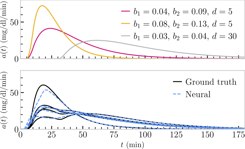
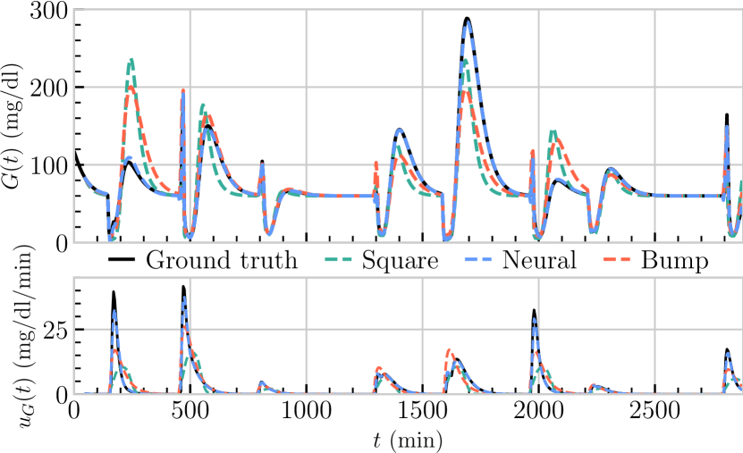
Figure 1: Left: (Top) “Absorption templates” used to generate $u_{G}$. (Bottom) 5 Samples of ground truth and learned $u_{G}$ for meals from the test set. Right: Glucose forecast and predicted absorption rates of each model over a 2 day window from the test trajectory.

	Exact timestamps		Noisy timestamps
$a_{i}$	Exact observations	Noisy observations	Exact observations	Noisy observations
Neural	0.95mg/dl	3.66mg/dl	1.48mg/dl	3.63mg/dl
Bump	9.52mg/dl	10.11mg/dl	9.53mg/dl	10.24mg/dl
Square	11.60mg/dl	11.53mg/dl	11.65mg/dl	11.56mg/dl

Table 1: Forecast RMSE computed over all possible 4 hour windows of the test set trajectory, reflecting the window size used for training.

Evaluations.

We compare our neural absorption function against the two common parameterizations of $u_{G}$ from Section 3, fit via gradient-based optimization. We approximate the piece-wise constant square function using a difference of sigmoids; otherwise the width cannot be learned. Our neural model is able to closely approximate the ground truth $u_{G}$, especially in the tails, as shown in Figure 1 (left). This results in significantly better forecasts, and our neural model closely tracks the ground truth glucose values and absorption rates, even extrapolating to durations much longer than what was seen in training. We visualize such long term forecasts in Figure 1 (right). We also report the forecast RMSE on the test set in Table 1. Our neural model attains lower forecast errors across all settings. In the noiseless case, our neural model is 10x more accurate than heuristic parameterizations. The RMSEs generally increase as we add noise, though the bump and square functions are already such poor forecasters that noise does not worsen their errors significantly.

5 Discussion

Our experiments show that our proposed method is a promising way to learn absorption profiles that depend on macronutritional information. Our approach readily generalizes to handle arbitrary meal covariates beyond macronutritional information, such as food images or descriptions. Although this paper only uses synthetic data, our method can complement any glucose dynamics model of real-world data. Learning accurate dynamics from data, however, remains a challenging problem. We see our method as a vital component in future data-driven hybrid models of glucose-insulin dynamics.

References

- Albers et al. [2020] D. J. Albers, M. E. Levine, M. Sirlanci, and A. M. Stuart. A Simple Modeling Framework For Prediction In The Human Glucose-Insulin System, August 2020.
- Albers et al. [2017] David J. Albers, Matthew Levine, Bruce Gluckman, Henry Ginsberg, George Hripcsak, and Lena Mamykina. Personalized glucose forecasting for type 2 diabetes using data assimilation. PLOS Computational Biology, 13(4):e1005232, April 2017. ISSN 1553-7358. doi: 10.1371/journal.pcbi.1005232.
- Andersen and Højbjerre [2003] Kim E. Andersen and Malene Højbjerre. A Bayesian Approach to Bergman’s Minimal Model. In International Workshop on Artificial Intelligence and Statistics, pages 1–8. PMLR, January 2003.
- Ayed et al. [2019] Ibrahim Ayed, Emmanuel de Bézenac, Arthur Pajot, Julien Brajard, and Patrick Gallinari. Learning Dynamical Systems from Partial Observations. CoRR, abs/1902.11136, 2019.
- Bergman et al. [1979] R N Bergman, Y Z Ider, C R Bowden, and C Cobelli. Quantitative estimation of insulin sensitivity. American Journal of Physiology-Endocrinology and Metabolism, 236(6):E667, June 1979. ISSN 0193-1849, 1522-1555. doi: 10.1152/ajpendo.1979.236.6.E667.
- Brajard et al. [2020] Julien Brajard, Alberto Carassi, Marc Bocquet, and Laurent Bertino. Combining data assimilation and machine learning to emulate a dynamical model from sparse and noisy observations: A case study with the Lorenz 96 model. Journal of Computational Science, 44:101171, July 2020. ISSN 18777503. doi: 10.1016/j.jocs.2020.101171.
- Chen et al. [2018] Ricky T. Q. Chen, Yulia Rubanova, Jesse Bettencourt, and David K Duvenaud. Neural Ordinary Differential Equations. In Advances in Neural Information Processing Systems, volume 31. Curran Associates, Inc., 2018.
- Chen et al. [2021] Yuming Chen, Daniel Sanz-Alonso, and Rebecca Willett. Auto-differentiable Ensemble Kalman Filters. arXiv:2107.07687 [cs, stat], July 2021.
- Dalla Man et al. [2006] C. Dalla Man, M. Camilleri, and C. Cobelli. A System Model of Oral Glucose Absorption: Validation on Gold Standard Data. IEEE Transactions on Biomedical Engineering, 53(12):2472–2478, December 2006. ISSN 0018-9294, 1558-2531. doi: 10.1109/TBME.2006.883792.
- Dalla Man et al. [2007] Chiara Dalla Man, Robert A. Rizza, and Claudio Cobelli. Meal Simulation Model of the Glucose-Insulin System. IEEE Transactions on Biomedical Engineering, 54(10):1740–1749, October 2007. ISSN 0018-9294. doi: 10.1109/TBME.2007.893506.
- Elashoff et al. [1982] Janet D. Elashoff, Terry J. Reedy, and James H. Meyer. Analysis of Gastric Emptying Data. Gastroenterology, 83(6):1306–1312, December 1982. ISSN 00165085. doi: 10.1016/S0016-5085(82)80145-5.
- Finzi et al. [2020] Marc Finzi, Ke Alexander Wang, and Andrew G. Wilson. Simplifying Hamiltonian and Lagrangian Neural Networks via Explicit Constraints. Advances in Neural Information Processing Systems, 33:13880–13889, 2020.
- Gallardo-Hernández et al. [2022] Ana Gabriela Gallardo-Hernández, Marcos A. González-Olvera, Medardo Castellanos-Fuentes, Jésica Escobar, Cristina Revilla-Monsalve, Ana Luisa Hernandez-Perez, and Ron Leder. Minimally-Invasive and Efficient Method to Accurately Fit the Bergman Minimal Model to Diabetes Type 2. Cellular and Molecular Bioengineering, 15(3):267–279, June 2022. ISSN 1865-5033. doi: 10.1007/s12195-022-00719-x.
- Herrero et al. [2012] Pau Herrero, Jorge Bondia, Cesar C. Palerm, Josep Vehí, Pantelis Georgiou, Nick Oliver, and Christofer Toumazou. A Simple Robust Method for Estimating the Glucose Rate of Appearance from Mixed Meals. Journal of Diabetes Science and Technology, 6(1):153–162, January 2012. ISSN 1932-2968, 1932-2968. doi: 10.1177/193229681200600119.
- Hovorka et al. [2004] Roman Hovorka, Valentina Canonico, Ludovic J Chassin, Ulrich Haueter, Massimo Massi-Benedetti, Marco Orsini Federici, Thomas R Pieber, Helga C Schaller, Lukas Schaupp, Thomas Vering, and Malgorzata E Wilinska. Nonlinear model predictive control of glucose concentration in subjects with type 1 diabetes. Physiological Measurement, 25(4):905–920, August 2004. ISSN 0967-3334, 1361-6579. doi: 10.1088/0967-3334/25/4/010.
- Hovorka et al. [2008] Roman Hovorka, Ludovic J Chassin, Martin Ellmerer, Johannes Plank, and Malgorzata E Wilinska. A simulation model of glucose regulation in the critically ill. Physiological measurement, 29(8):959, 2008.
- Kemeth et al. [2021] Felix P. Kemeth, Tom Bertalan, Nikolaos Evangelou, Tianqi Cui, Saurabh Malani, and Ioannis G. Kevrekidis. Initializing LSTM internal states via manifold learning. Chaos: An Interdisciplinary Journal of Nonlinear Science, 31(9):093111, September 2021. ISSN 1054-1500, 1089-7682. doi: 10.1063/5.0055371.
- Kingma and Ba [2014] Diederik P. Kingma and Jimmy Ba. Adam: A method for stochastic optimization, 2014. URL https://arxiv.org/abs/1412.6980.
- Levine and Stuart [2022] Matthew E. Levine and Andrew M. Stuart. A framework for machine learning of model error in dynamical systems. Communications of the American Mathematical Society, 2(07):283–344, 2022. ISSN 2692-3688. doi: 10.1090/cams/10.
- [20] Chengyuan Liu, Josep Vehı, Nick Oliver, Pantelis Georgiou, and Pau Herrero. Enhancing Blood Glucose Prediction with Meal Absorption and Physical Exercise Information. page 10.
- Mari et al. [2020] Andrea Mari, Andrea Tura, Eleonora Grespan, and Roberto Bizzotto. Mathematical Modeling for the Physiological and Clinical Investigation of Glucose Homeostasis and Diabetes. Frontiers in Physiology, 11:575789, November 2020. ISSN 1664-042X. doi: 10.3389/fphys.2020.575789.
- Miller et al. [2021] Andrew C. Miller, Nicholas J. Foti, and Emily B. Fox. Breiman’s Two Cultures: You Don’t Have to Choose Sides. Observational Studies, 7(1):161–169, 2021. ISSN 2767-3324. doi: 10.1353/obs.2021.0003.
- Ouala et al. [2020] S. Ouala, D. Nguyen, L. Drumetz, B. Chapron, A. Pascual, F. Collard, L. Gaultier, and R. Fablet. Learning latent dynamics for partially observed chaotic systems. Chaos: An Interdisciplinary Journal of Nonlinear Science, 30(10):103121, October 2020. ISSN 1054-1500, 1089-7682. doi: 10.1063/5.0019309.
- Rico-Martinez et al. [1994] R. Rico-Martinez, J.S. Anderson, and I.G. Kevrekidis. Continuous-time nonlinear signal processing: A neural network based approach for gray box identification. In Proceedings of IEEE Workshop on Neural Networks for Signal Processing, pages 596–605, Ermioni, Greece, 1994. IEEE. ISBN 978-0-7803-2026-0. doi: 10.1109/NNSP.1994.366006.
- Rubanova et al. [2019] Yulia Rubanova, Ricky T. Q. Chen, and David K Duvenaud. Latent Ordinary Differential Equations for Irregularly-Sampled Time Series. In Advances in Neural Information Processing Systems, volume 32. Curran Associates, Inc., 2019.
- Sturis et al. [1991] Jeppe Sturis, Kenneth S Polonsky, Erik Mosekilde, and Eve Van Cauter. Computer model for mechanisms underlying ultradian oscillations of insulin and glucose. American Journal of Physiology-Endocrinology And Metabolism, 260(5):E801–E809, 1991.
- Willard et al. [2022] Jared Willard, Xiaowei Jia, Shaoming Xu, Michael Steinbach, and Vipin Kumar. Integrating Scientific Knowledge with Machine Learning for Engineering and Environmental Systems. ACM Computing Surveys, page 3514228, March 2022. ISSN 0360-0300, 1557-7341. doi: 10.1145/3514228.
- Zeevi et al. [2015] David Zeevi, Tal Korem, Niv Zmora, David Israeli, Daphna Rothschild, Adina Weinberger, Orly Ben-Yacov, Dar Lador, Tali Avnit-Sagi, Maya Lotan-Pompan, Jotham Suez, Jemal Ali Mahdi, Elad Matot, Gal Malka, Noa Kosower, Michal Rein, Gili Zilberman-Schapira, Lenka Dohnalová, Meirav Pevsner-Fischer, Rony Bikovsky, Zamir Halpern, Eran Elinav, and Eran Segal. Personalized Nutrition by Prediction of Glycemic Responses. Cell, 163(5):1079–1094, November 2015. ISSN 00928674. doi: 10.1016/j.cell.2015.11.001.