Structured interpolation for multivariate transfer functions of quadratic-bilinear systems

Abstract

High-dimensional/high-fidelity nonlinear dynamical systems appear naturally when the goal is to accurately model real-world phenomena. Many physical properties are thereby encoded in the internal differential structure of these resulting large-scale nonlinear systems. The high-dimensionality of the dynamics causes computational bottlenecks, especially when these large-scale systems need to be simulated for a variety of situations such as different forcing terms. This motivates model reduction where the goal is to replace the full-order dynamics with accurate reduced-order surrogates. Interpolation-based model reduction has been proven to be an effective tool for the construction of cheap-to-evaluate surrogate models that preserve the internal structure in the case of weak nonlinearities. In this paper, we consider the construction of multivariate interpolants in frequency domain for structured quadratic-bilinear systems. We propose definitions for structured variants of the symmetric subsystem and generalized transfer functions of quadratic-bilinear systems and provide conditions for structure-preserving interpolation by projection. The theoretical results are illustrated using two numerical examples including the simulation of molecular dynamics in crystal structures.

We introduce new formulas for structured subsystem transfer functions to describe quadratic-bilinear systems with internal differential structures in the frequency domain. We formulate conditions on projection spaces to enforce structure-preserving interpolation for such transfer functions allowing for structure-preserving model reduction of quadratic-bilinear systems.

1 Introduction

The accurate modeling of real-world phenomena and processes yields dynamical systems typically including nonlinearities. Additionally, these systems often inherit some internal structure from the underlying physical nature of the considered problem. An example for such internal structures is the description of internal system states by second-order time derivatives as it is usually the case in the modeling of mechanical structures. Such nonlinear mechanical systems take the form

$$\widetilde{M}\ddot{q}(t) =f\big{(}q(t),\dot{q}(t),u(t)\big{)},$$ (1)

$$y(t) =C_{\mathrm{p}}q(t)+C_{\mathrm{v}}\dot{q}(t),$$

with internal states $q(t)\in\mathbb{R}^{\ell}$, describing the system behavior, the external controls $u(t)\in\mathbb{R}^{m}$ that allow the user to change the internal behavior, and the quantities of interest $y(t)\in\mathbb{R}^{p}$ that can be observed from the outside, e.g., by sensor measurements. Thereby, the first equation in Eq. 1 is a second-order differential equation with mass (descriptor) matrix $\widetilde{M}\in\mathbb{R}^{\ell\times\ell}$ and the nonlinear time evolution function $f\colon\mathbb{R}^{\ell}\times\mathbb{R}^{\ell}\times\mathbb{R}^{m}\to\mathbb{R}^{\ell}$. The second, algebraic equation describes the quantities of interest as linear combination of the states and their first-order derivatives. Throughout this paper, we assume for any system to have homogeneous initial conditions.

The Toda lattice is an example of a nonlinear mechanical system of the form Eq. 1. It is used in solid state mechanics to model the movement of particles in a one-dimensional crystal structure [33]; see Figure 1. The nonlinear time evolution function contains exponential terms that describe the forces between the different particles:

$$f\big{(}q(t),\dot{q}(t),u(t)\big{)}=-\widetilde{D}\dot{q}(t)-\begin{bmatrix}e^{k_{1}(q_{1}(t)-q_{2}(t))}-1\\ e^{k_{2}(q_{2}(t)-q_{3}(t))}-e^{k_{1}(q_{1}(t)-q_{2}(t))}\\ \vdots\\ e^{k_{\ell}q_{\ell}(t)}-e^{k_{\ell-1}(q_{\ell-1}(t)-q_{\ell}(t))}\end{bmatrix},$$ (2)

with the positive semidefinite diagonal damping matrix $\widetilde{D}\in\mathbb{R}^{\ell\times\ell}$ and the positive stiffness coefficients $k_{1},\ldots,k_{\ell}$. See [35, Sec. 1.3.3] for the derivation of the differential model from the underlying Hamiltonian.

Figure 1: Schematic illustration of the Toda lattice with $\ell$ particles [35]. Atoms in a one-dimensional crystal structure are represented as point masses and connected by exponential springs modeling the forces between the particles.

In many applications, in particular those involving discretizations of partial differential equations, the number of differential equations $\ell$ in Eq. 1, describing the internal system behavior, is large and increases further with the demand for more accuracy. However, an increasing amount of differential equations also leads to an increasing demand for computational resources such as time and memory for simulations of the models or their use in optimization. A remedy to this problem is model order reduction, which aims for the computation of cheap-to-evaluate surrogate models described by significantly less differential equations, $r\ll\ell$, which approximate the input-to-output behavior of the original system as

$$\lVert y-\hat{y}\rVert\leq\tau\cdot\lVert u\rVert,$$

in some suitable norms for the output of the reduced model $\hat{y}$ and all admissible inputs $u$.

An established approach for model reduction of general (structured) nonlinear systems such as Eq. 1 is proper orthogonal decomposition (POD) [20, 23, 37], in which time simulations are used to extract information about the system dynamics for the construction of a basis matrix to project the system states. Other approaches aim for the extension of balancing-related model reduction to nonlinear systems using Gramians defined via time simulations as in the empirical Gramian method [19, 24, 25] or by new energy measures [32, 21] to construct suitable projection matrices. Nevertheless, a problem arising in the general system case is the approximation of the nonlinear time evolution function $f$ in Eq. 1 that circumvents the computationally expensive lifting and truncation of the low-dimensional state in every time step. A solution to that are hyperreduction techniques such as the (discrete) empirical interpolation method ((D)EIM) [4, 12, 13, 27], which computes a selection operator to restrict the evaluation of $f$ to its rows most contributing. This introduces another layer of approximations and needs explicit access to the implementation of the original time evolution function $f$.

An alternative to hyperreduction that gained significant popularity in model reduction in the last decade is quadratic-bilinearization [18]; in optimization also known as McCormick relaxation [26]: For $f$ smooth enough, general nonlinear systems can be rewritten into quadratic-bilinear form by introducing auxiliary variables and differential-algebraic equations, which then can be reduced directly using the classical projection-based model reduction approach. In the case of Eq. 1, the corresponding quadratic-bilinear system retains the internal mechanical structure as

$$0 =M\ddot{q}(t)+D\dot{q}(t)+Kq(t)$$ (3)

$$\quad{}+{}H_{\mathrm{vv}}\big{(}\dot{q}(t)\otimes\dot{q}(t)\big{)}+H_{\mathrm{vp}}\big{(}\dot{q}(t)\otimes q(t)\big{)}$$

$$\quad{}+{}H_{\mathrm{pv}}\big{(}q(t)\otimes\dot{q}(t)\big{)}+H_{\mathrm{pp}}\big{(}q(t)\otimes q(t)\big{)}$$

$$\quad{}-{}\sum_{j=1}^{m}N_{\mathrm{v},j}\dot{q}(t)u_{j}(t)-\sum_{j=1}^{m}N_{\mathrm{p},j}q(t)u_{j}(t)-B_{\mathrm{u}}u(t),$$

$$y(t) =C_{\mathrm{p}}q(t)+C_{\mathrm{v}}\dot{q}(t),$$

where $M,D,K,N_{\mathrm{v},j},N_{\mathrm{p},j}\in\mathbb{R}^{n\times n}$, for $j=1,\ldots,m$, $H_{\mathrm{vv}},H_{\mathrm{vp}},H_{\mathrm{pv}},H_{\mathrm{pp}}\in\mathbb{R}^{n\times n^{2}}$, $B_{\mathrm{u}}\in\mathbb{R}^{n\times m}$, $C_{\mathrm{p}},C_{\mathrm{v}}\in\mathbb{R}^{p\times n}$, and $\otimes$ denotes the Kronecker product. Due to the introduction of auxiliary variables, we have that $n\geq\ell$, which appears counter-intuitive to the actual task of reducing the number of internal system states in model reduction. However, the new nonlinearity structure of Eq. 3 allows to apply well-established model reduction techniques without the necessity of the hyperreduction step for the nonlinearity. The Toda lattice model (Figure 1) can also be rewritten into Eq. 3. The process of quadratic-bilinearization and the derivation of several structured quadratic-bilinear formulations for the Toda lattice model are shown in [35, Sec. 6.2]. Furthermore, we refer the reader to the numerical experiments in Section 5.3 for more details.

So far, the literature on the model reduction of quadratic-bilinear systems mainly considered the case of unstructured, first-order systems of the form

$$E\dot{x}(t) =Ax(t)+H\big{(}x(t)\otimes x(t)\big{)}+\sum\limits_{j=1}^{m}Nx(t)u_{j}(t)+Bu(t),$$ (4)

$$y(t) =Cx(t),$$

with $E,A,N_{j}\in\mathbb{R}^{n\times n}$, for $j=1,\ldots,m$, $H\in\mathbb{R}^{n\times n^{2}}$, $B\in\mathbb{R}^{n\times m}$ and $C\in\mathbb{R}^{p\times n}$. Model reduction methods developed for Eq. 4 among others include the interpolation of multivariate subsystem transfer functions [18, 1, 6, 2], Volterra series interpolation [9, 2], balanced truncation [7], learning models from frequency domain data via the Loewner framework [15] or learning models from time domain data by operator inference [28, 29]. The reformulation of general nonlinear systems into quadratic-bilinear form Eq. 4 has also been proven to be an effective strategy for classical nonlinear model reduction methods such as POD [22].

In this paper, we extend the idea of quadratic-bilinear subsystem interpolation to systems with additional internal differential structures such as in the mechanical case Eq. 3. We propose extensions for the definitions of the first three symmetric subsystem transfer functions and the first three generalized transfer functions to the structured system case and then present subspace conditions for structure-preserving interpolation of these transfer functions. The effectiveness of resulting model reduction methods based on this interpolation theory is illustrated on two different structured examples including the Toda lattice model above. Parts of the theoretical results presented here were derived in the course of writing the dissertation of the corresponding author [35].

The rest of the paper is organized as follows: In Section 2, we recap the ideas of Volterra series expansions and unstructured quadratic-bilinear systems in the frequency domain. We present the definitions of structured transfer functions of quadratic-bilinear systems in Section 3 and the results on structure-preserving interpolation in Section 4. We employ the interpolation results for model reduction of two structured numerical examples in Section 5. The paper is concluded in Section 6.

2 Mathematical preliminaries

In this section, we recap the concept of Volterra series for quadratic-bilinear systems and two resulting transfer function formulations.

2.1 Volterra series expansions

The Volterra series expansion allows to describe the solution of nonlinear dynamical systems as a series of solutions of coupled linear systems [31]. A common approach to derive the Volterra series expansion is by variational analysis [18]. Let a scaled input signal $\alpha u(t)$, with $\alpha>0$, be given for the quadratic-bilinear system Eq. 4 and assume the system state to have an analytic representation of the form

$$x(t)=\sum\limits_{k=1}^{\infty}\alpha^{k}x_{k}(t),$$ (5)

with a sequence of states $x_{k}(t)$. Inserting Eq. 5 into Eq. 4 and extracting the terms corresponding to the same power of the coefficient $\alpha$ yields the states $x_{k}(t)$ to be described by cascaded subsystems, which are linear in their respective unknown state $x_{k}(t)$. For example, the first three resulting linear subsystems for Eq. 5 are given by

$$E\dot{x}_{1}(t) =Ax_{1}(t)+Bu(t),$$ (6)

$$E\dot{x}_{2}(t) =Ax_{2}(t)+H\big{(}x_{1}(t)\otimes x_{1}(t)\big{)}+\sum\limits_{j=1}^{m}N_{j}x_{1}(t)u_{j}(t),$$

$$E\dot{x}_{3}(t) =Ax_{3}(t)+H\big{(}x_{1}(t)\otimes x_{2}(t)+x_{2}(t)\otimes x_{1}(t)\big{)}+\sum\limits_{j=1}^{m}N_{j}x_{2}(t)u_{j}(t).$$

Applying the variation-of-constants formula to the subsystems in Eq. 6 allows the description of the input-to-output behavior of Eq. 4 via its Volterra series expansion:

$$y(t)=\sum\limits_{k=1}^{\infty}\int\limits_{0}^{t}\int\limits_{0}^{t_{1}}\cdots\int\limits_{0}^{t_{k-1}}g_{k}(t_{1},\ldots,t_{k})\big{(}u(t-t_{1})\otimes\cdots\otimes u(t-t_{k})\big{)}\operatorname{d}{t_{k}}\cdots\operatorname{d}{t_{1}},$$ (7)

where $g_{k}(t_{1},\ldots,t_{k})$ are the Volterra kernels of the corresponding representation. The kernels used in Eq. 7 are of the symmetric type [31, 18]. Applying the multivariate Laplace transformation [31] to Eq. 7 results in an equivalent description of the quadratic-bilinear system Eq. 4 in the frequency domain by multivariate transfer functions.

2.2 Subsystem transfer functions of quadratic-bilinear systems

In this work, we restrict ourselves to the presentation of the transfer functions corresponding to the first three coupled linear subsystems for brevity and practical relevance. General formulas for arbitrarily high levels of multivariate transfer functions for Eq. 4 have been developed in [35, Sec. 2.3.2].

2.2.1 Symmetric subsystem transfer functions

The symmetric subsystem transfer functions are based on the symmetric Volterra kernels from [31]; cf. Eq. 7. Historically, this is the first transfer function type that has been investigated for the model reduction of Eq. 4 in [18]. Here, the term “symmetric” refers to the fact that the transfer function is invariant with respect to the order of its arguments.

The first symmetric subsystem transfer function corresponds to the linear part of Eq. 4 as it can be seen in Eq. 6 such that

$$G_{\mathrm{sym},1}(s_{1})=Cg_{\mathrm{sym},1}(s_{1})=C(s_{1}E-A)^{-1}B,$$ (8)

with $s_{1}\in\mathbb{C}$. Thereby, the term $g_{\mathrm{sym},1}(s_{1})\in\mathbb{C}^{n\times m}$ is used in the following for notational convenience and denotes the input-to-state transition of the first subsystem. The second symmetric subsystem transfer function depends on two complex frequency arguments $s_{1},s_{2}\in\mathbb{C}$ and is given by

$$G_{\mathrm{sym},2}(s_{1},s_{2})=Cg_{\mathrm{sym},2}(s_{1},s_{2}),$$ (9)

where the function describing the input-to-state transition on the right-hand side of Eq. 9 is given by

$$g_{\mathrm{sym},2}(s_{1},s_{2}) =\frac{1}{2}\big{(}(s_{1}+s_{2})E-A\big{)}^{-1}$$

$$\quad{}\times{}\Big{(}H\big{(}g_{\mathrm{sym},1}(s_{1})\otimes g_{\mathrm{sym},1}(s_{2})+g_{\mathrm{sym},1}(s_{2})\otimes g_{\mathrm{sym},1}(s_{1})\big{)}$$

$$\qquad{}+{}N\big{(}I_{m}\otimes\big{(}g_{\mathrm{sym},1}(s_{1})+g_{\mathrm{sym},1}(s_{2})\big{)}\big{)}\Big{)},$$

with $g_{\mathrm{sym},1}$ from Eq. 8, $I_{m}$ denoting the $m$-dimensional identity matrix and the column concatenation of the bilinear terms as

$$N=\begin{bmatrix}N_{1}&N_{2}&\ldots&N_{m}\end{bmatrix}.$$ (10)

Last, the third symmetric subsystem transfer function is defined similarly to Eq. 9 by

$$G_{\mathrm{sym},3}(s_{1},s_{2},s_{3})=Cg_{\mathrm{sym},3}(s_{1},s_{2},s_{3}),$$ (11)

with $s_{1},s_{2},s_{3}\in\mathbb{C}$ and the input-to-state transition given via

$$g_{\mathrm{sym},3}(s_{1},s_{2},s_{3}) =\frac{1}{6}\big{(}(s_{1}+s_{2}+s_{3})E-A\big{)}^{-1}$$

$$\quad{}\times{}\Big{(}H\big{(}g_{\mathrm{sym},1}(s_{1})\otimes g_{\mathrm{sym},2}(s_{2},s_{3})+g_{\mathrm{sym},1}(s_{2})\otimes g_{\mathrm{sym},2}(s_{1},s_{3})$$

$$\quad\qquad{}+{}g_{\mathrm{sym},1}(s_{3})\otimes g_{\mathrm{sym},2}(s_{1},s_{2})+g_{\mathrm{sym},2}(s_{1},s_{2})\otimes g_{\mathrm{sym},1}(s_{3})$$

$$\quad\qquad{}+{}g_{\mathrm{sym},2}(s_{1},s_{3})\otimes g_{\mathrm{sym},1}(s_{2})+g_{\mathrm{sym},2}(s_{2},s_{3})\otimes g_{\mathrm{sym},1}(s_{1})\big{)}$$

$$\qquad{}+{}N\big{(}I_{m}\otimes\big{(}g_{\mathrm{sym},2}(s_{1},s_{2})+g_{\mathrm{sym},2}(s_{1},s_{3})+g_{\mathrm{sym},2}(s_{2},s_{3})\big{)}\big{)}\Big{)},$$

using $g_{\mathrm{sym},1}$ from Eq. 8 and $g_{\mathrm{sym},2}$ from Eq. 9.

2.2.2 Generalized transfer functions

In contrast to the symmetric case, the generalized transfer functions do not directly correspond to a Volterra kernel representation. They have been introduced in [15] for the extension of the data-driven Loewner framework to quadratic-bilinear systems and are inspired by the regular transfer functions of bilinear systems, which only consist of products of the terms of the dynamical system; see, e.g., [3]. The formulation given in [15] for the single-input/single-output (SISO) system case has been extended to multi-input/multi-output systems in [35, Sec. 2.3.2].

As in the symmetric case, the first regular transfer function corresponds to the linear system components, with

$$G_{\mathrm{gen},1}^{\mathrm{(B)}}(s_{1})=C(s_{1}E-A)^{-1}B.$$ (12)

Also the second regular transfer function is uniquely defined resulting from one multiplication with the bilinear terms:

$$G_{\mathrm{gen},2}^{\mathrm{(N,(B))}}(s_{1},s_{2})=C(s_{2}E-A)^{-1}N\big{(}I_{m}\otimes(s_{1}E-A)^{-1}B\big{)}.$$ (13)

For the third level however, two different generalized transfer functions exist. The first one is identical to the third regular bilinear transfer function with

$$G_{\mathrm{gen},3}^{\mathrm{(N,(N,(B)))}}(s_{1},s_{2},s_{3}) =C(s_{3}E-A)^{-1}N\Big{(}I_{m}\otimes\big{(}(s_{2}E-A)^{-1}N$$ (14)

$$\quad{}\otimes{}(I_{m}\otimes(s_{1}E-A)^{-1}B)\big{)}\Big{)};$$

see also [10]. The second one involves the quadratic term and is given by

$$G_{\mathrm{gen},3}^{\mathrm{(H,(B),(B))}}(s_{1},s_{2},s_{3})=C(s_{3}E-A)^{-1}H\big{(}(s_{2}E-A)^{-1}B\otimes(s_{1}E-A)^{-1}B\big{)}.$$ (15)

Note that the index levels of the generalized and symmetric transfer functions do not coincide since the second symmetric subsystem transfer function does contain the quadratic term in contrast to the second level generalized transfer function, which has only the bilinear terms.

3 Structured transfer functions of quadratic-bilinear systems

In this section, we extend the transfer function formulations from Section 2 to the setting of structured quadratic-bilinear systems starting with the introductory example of quadratic-bilinear mechanical systems. Based on this motivation, we introduce the formulas for structured symmetric and generalized transfer functions before we consider the case of quadratic-bilinear time-delay systems as another example for internal differential structures at the end of this section.

3.1 Transfer functions for mechanical systems

In general, any system in second-order form Eq. 3 can be rewritten in first-order form Eq. 4 using the concatenated first-order state $x(t)=\begin{bmatrix}q(t)^{\mkern-1.5mu\mathsf{T}}&\dot{q}(t)^{\mkern-1.5mu\mathsf{T}}\end{bmatrix}^{\mkern-1.5mu\mathsf{T}}$. The first-order system matrices are then, for example, given by

$$E =\begin{bmatrix}I_{n}&0\\ 0&M\end{bmatrix}, A =\begin{bmatrix}0&I_{n}\\ -K&-D\end{bmatrix}, B =\begin{bmatrix}0\\ B_{\mathrm{u}}\end{bmatrix},$$ (16)

$$C =\begin{bmatrix}C_{\mathrm{p}}&C_{\mathrm{v}}\end{bmatrix}, N_{j} =\begin{bmatrix}0&0\\ N_{\mathrm{p},j}&N_{\mathrm{v},j}\end{bmatrix},$$

for $j=1,\ldots,m$, with the quadratic term

$$H=-\begin{bmatrix}0&0&\ldots&0&0&0&0&\ldots&0&0\\ H_{\mathrm{pp},1}&H_{\mathrm{pv},1}&\ldots&H_{\mathrm{pp},n}&H_{\mathrm{pv},n}&H_{\mathrm{vp},1}&H_{\mathrm{vv},1}&\ldots&H_{\mathrm{vp},n}&H_{\mathrm{vv},n}\end{bmatrix}.$$ (17)

Thereby, the matrix blocks in Eq. 17 are $n\times n$ matrix slices of the second-order quadratic terms in Eq. 3, e.g., for $H_{\mathrm{pp}}$ modeling the multiplication of the state with itself we have

$$H_{\mathrm{pp}}=\begin{bmatrix}H_{\mathrm{pp},1}&H_{\mathrm{pp},2}&\ldots&H_{\mathrm{pp},n}\end{bmatrix},$$

with $H_{\mathrm{pp},j}\in\mathbb{R}^{n\times n}$ for all $j=1,\ldots,n$.

Now, we exploit the block structures of the matrices in Eqs. 16 and 17 to derive the symmetric and generalized transfer functions of Eq. 3. In both transfer function cases, the first level transfer functions correspond to the linear system case and it can be observed that for Eq. 3 it holds that

$$G_{\mathrm{sym},1}(s_{1})=G_{\mathrm{gen},1}^{\mathrm{(B)}}(s_{1}) =(C_{\mathrm{p}}+s_{1}C_{\mathrm{v}})g_{\mathrm{sym},1}(s_{1})$$ (18)

$$=(C_{\mathrm{p}}+s_{1}C_{\mathrm{v}})(s_{1}^{2}M+s_{1}D+K)^{-1}B_{\mathrm{u}},$$

where $g_{\mathrm{sym},1}(s_{1})$ denotes here the input-to-state transition of the second-order state $q$.

For the next two levels, we concentrate first on the symmetric transfer function case. Inserting Eqs. 16 and 17 into Eq. 9 yields the second symmetric subsystem transfer function of Eq. 3 to be

$$G_{\mathrm{sym},2}(s_{1},s_{2}) =\big{(}C_{\mathrm{p}}+(s_{1}+s_{2})C_{\mathrm{v}}\big{)}g_{\mathrm{sym},2}(s_{1},s_{2})$$ (19)

$$=\frac{1}{2}\big{(}C_{\mathrm{p}}+(s_{1}+s_{2})C_{\mathrm{v}}\big{)}\big{(}(s_{1}+s_{2})^{2}M+(s_{1}+s_{2})D+K\big{)}^{-1}$$

$$\quad{}\times{}\Big{(}-(H_{\mathrm{pp}}+s_{2}H_{\mathrm{pv}}+s_{1}H_{\mathrm{vp}}+s_{1}s_{2}H_{\mathrm{vv}})\big{(}g_{\mathrm{sym},1}(s_{1})\otimes g_{\mathrm{sym},1}(s_{2})\big{)}$$

$$\qquad{}-{}(H_{\mathrm{pp}}+s_{1}H_{\mathrm{pv}}+s_{2}H_{\mathrm{vp}}+s_{1}s_{2}H_{\mathrm{vv}})\big{(}g_{\mathrm{sym},1}(s_{2})\otimes g_{\mathrm{sym},1}(s_{1})\big{)}$$

$$\qquad{}+{}(N_{\mathrm{p}}+s_{1}N_{\mathrm{v}})\big{(}I_{m}\otimes g_{\mathrm{sym},1}(s_{1})\big{)}$$

$$\qquad{}+{}(N_{\mathrm{p}}+s_{2}N_{\mathrm{v}})\big{(}I_{m}\otimes g_{\mathrm{sym},1}(s_{2})\big{)}\Big{)},$$

where $g_{\mathrm{sym},2}$ denotes the input-to-state transition of the second subsystem, $g_{\mathrm{sym},1}$ is the input-to-state transition from the first subsystem in Eq. 18, and the bilinear terms are concatenated as

$$N_{\mathrm{p}} =\begin{bmatrix}N_{\mathrm{p},1}&\ldots&N_{\mathrm{p},m}\end{bmatrix} N_{\mathrm{v}} =\begin{bmatrix}N_{\mathrm{v},1}&\ldots&N_{\mathrm{v},m}\end{bmatrix}.$$ and (20)

Similarly, inserting the block matrices Eqs. 16 and 17 into the unstructured third symmetric subsystem transfer function Eq. 11 leads to the structured third symmetric subsystem transfer function representation for Eq. 3. Due to the complexity of the resulting formula, we will not write it out here explicitly but outline some of its features. The third subsystem transfer function of Eq. 4 has a similar structure to Eqs. 11 and 19 with linear combinations of the quadratic and bilinear terms multiplied with the previous input-to-state transition terms $g_{\mathrm{sym},1}$ and $g_{\mathrm{sym},2}$ from Eqs. 18 and 19. Due to the occurrence of the sum of the frequency arguments in the first term of Eq. 19, this translates into the frequency dependence of the second-order quadratic and bilinear terms such that terms of the forms

$$-\big{(}H_{\mathrm{pp}}+s_{3}H_{\mathrm{pv}}+(s_{1}+s_{2})H_{\mathrm{vp}}+(s_{1}+s_{2})s_{3}H_{\mathrm{vv}}\big{)}\big{(}g_{\mathrm{sym},2}(s_{1},s_{2})\otimes g_{\mathrm{sym},1}(s_{3})\big{)}$$ (21)

$$\text{and}\quad\big{(}N_{\mathrm{p}}+(s_{1}+s_{2})N_{\mathrm{v}}\big{)}\big{(}I_{m}\otimes g_{\mathrm{sym},2}(s_{1},s_{2})\big{)}$$

appear. For more details, we refer the reader to the next section, which contains the definitions of the transfer function formulas for general structures.

For the generalized transfer functions, one can observe that the second level transfer function resembles the corresponding bilinear regular transfer function, for which the structured system case has been developed in [10]. The resulting transfer function for Eq. 3 is thereby given as

$$G_{\mathrm{gen},2}^{\mathrm{(N,(B))}}(s_{1},s_{2}) =(C_{\mathrm{p}}+s_{2}C_{\mathrm{v}})(s_{2}^{2}M+s_{2}D+K)^{-1}(N_{\mathrm{p}}+s_{1}N_{\mathrm{v}})$$ (22)

$$\quad{}\times{}\big{(}I_{m}\otimes(s_{1}^{2}M+s_{1}D+K)^{-1}B_{\mathrm{u}}\big{)},$$

where the bilinear terms are concatenated as in Eq. 20. Similarly, the purely bilinear third level generalized transfer function of Eq. 3 is given by

$$G_{\mathrm{gen},3}^{\mathrm{(N,(N,(B)))}} =(C_{\mathrm{p}}+s_{3}C_{\mathrm{v}})(s_{3}^{2}M+s_{3}D+K)^{-1}(N_{\mathrm{p}}+s_{2}N_{\mathrm{v}})$$ (23)

$$\quad{}\times{}\Big{(}I_{m}\otimes(s_{2}^{2}M+s_{2}D+K)^{-1}(N_{\mathrm{p}}+s_{1}N_{\mathrm{v}})$$

$$\qquad{}\times{}\big{(}I_{m}\otimes(s_{1}^{2}M+s_{1}D+K)^{-1}B_{\mathrm{u}}\big{)}\Big{)}.$$

On the other hand, the third level generalized transfer function of Eq. 3 involving the quadratic term can be derived by inserting Eq. 16 into Eq. 15, which yields

$$G_{\mathrm{gen},3}^{\mathrm{(H,(B),(B))}}(s_{1},s_{2},s_{3}) =-(C_{\mathrm{p}}+s_{3}C_{\mathrm{v}})(s_{3}^{2}M+s_{3}D+K)^{-1}$$ (24)

$$\quad{}\times{}(H_{\mathrm{pp}}+s_{1}H_{\mathrm{pv}}+s_{2}H_{\mathrm{vp}}+s_{1}s_{2}H_{\mathrm{vv}})$$

$$\quad{}\times{}\big{(}(s_{2}^{2}M+s_{2}D+K)^{-1}B_{\mathrm{u}}\otimes(s_{1}^{2}M+s_{1}D+K)^{-1}B_{\mathrm{u}}\big{)}.$$

Overall, and similar to the linear and bilinear cases, we can observe the occurrence of the same terms describing the linear, bilinear or quadratic dynamics in the different transfer functions by means of the given system matrices and the complex variables $s_{1},s_{2},s_{3}$. This motivates the definitions for the general structured framework in the upcoming section.

3.2 Structured transfer function formulas for quadratic-bilinear systems

Before deriving structured quadratic-bilinear transfer functions, we briefly recall the ideas from [5], which considered the structured transfer functions for linear dynamical systems in which frequency-dependent equations are used for describing the dynamics. First, consider linear first-order (unstructured) systems with the time domain representation

$$E\dot{x}(t)-Ax(t) =Bu(t), y(t)=Cx(t).$$ (25)

By taking the Laplace transform of Eq. 25, the dynamical system in Eq. 25 can be equivalently described in the frequency domain as

$$(sE-A)X(s) =BU(s), Y(s)=CX(s),$$ (26)

with $s\in\mathbb{C}$, where $U(s),X(s),Y(s)$ are the Laplace transforms of the inputs $u(t)$, states $x(t)$, and outputs $y(t)$, respectively. Now consider a linear dynamical system with a second-order structure with the time domain representation

$$M\ddot{x}(t)+D\dot{x}(t)+Kx(t) =B_{\mathrm{u}}u(t), y(t)=C_{\mathrm{p}}x(t)+C_{\mathrm{v}}\dot{x}(t).$$ (27)

As in the unstructured case, taking the Laplace transform of Eq. 27 yields the representation in the frequency domain

$$(s^{2}M+sD+K)X(s) =B_{\mathrm{u}}U(s), Y(s)=(C_{\mathrm{p}}+sC_{\mathrm{v}})X(s).$$ (28)

Observe that in both cases of Eq. 26 and Eq. 28, the system states in the frequency domain can be described as solution of frequency-dependent linear systems of equations of the form

$$\mathcal{K}(s)X(s) =\mathcal{B}(s)U(s), Y(s) =\mathcal{C}(s),$$ (29)

where the matrix-valued functions $\mathcal{K}\colon\mathbb{C}\to\mathbb{C}^{n\times n}$, $\mathcal{B}\colon\mathbb{C}\to\mathbb{C}^{n\times m}$ and $\mathcal{C}\colon\mathbb{C}\to\mathbb{C}^{p\times m}$ describe the linear dynamics, and the input and output behavior of the system. In particular, we recover Eq. 26 by setting $\mathcal{K}(s)=sE-A$, $\mathcal{B}(s)=B$, and $\mathcal{C}(s)=B$. Similarly, we recover Eq. 28 by setting $\mathcal{K}(s)=s^{2}M+sD+K$, $\mathcal{B}(s)=B_{\mathrm{u}}$, and $\mathcal{C}(s)=C_{\mathrm{p}}+sC_{\mathrm{v}}$. We refer the reader to [5] for further examples of structured dynamics that fit into the general framework of Eq. 29. Then, for every $s\in\mathbb{C}$ for which $\mathcal{K}(s)$ in Eq. 29 is invertible, the transfer function of the underlying linear dynamical system is given by

$$G(s)=\mathcal{C}(s)\mathcal{K}(s)^{-1}\mathcal{B}(s).$$ (30)

For the extension to structured bilinear systems in [10], a new frequency-dependent function $\mathcal{N}\colon\mathbb{C}\to\mathbb{C}^{n\times nm}$ was introduced, modeling the effect of the bilinear terms, where

$$\mathcal{N}(s)=\begin{bmatrix}\mathcal{N}_{1}(s)&\ldots&\mathcal{N}_{m}(s)\end{bmatrix},$$

with $\mathcal{N}_{j}\colon\mathbb{C}\to\mathbb{C}^{n\times n}$ for all $j=1,\ldots,m$. In this manuscript, we further extend the structured transfer function framework to the quadratic-bilinear case, which appears ubiquitously in prominent applications as we briefly discussed in Section 1.

First, we consider the symmetric transfer function case. Inspired by Eqs. 8, 9 and 11, from the unstructured first-order case, and Eqs. 18, 19 and 21, we introduce the following definition for the structured symmetric subsystem transfer functions.

Definition 1.

Given matrix-valued functions of the form $\mathcal{C}\colon\mathbb{C}\to\mathbb{C}^{p\times m}$, $\mathcal{K}\colon\mathbb{C}\to\mathbb{C}^{n\times n}$, $\mathcal{B}\colon\mathbb{C}\to\mathbb{C}^{n\times m}$, $\mathcal{N}\colon\mathbb{C}\to\mathbb{C}^{n\times nm}$, $\mathcal{H}\colon\mathbb{C}\times\mathbb{C}\to\mathbb{C}^{n\times n^{2}}$, for which there exists an $s\in\mathbb{C}$ at which they can be evaluated and $\mathcal{K}(s)$ is invertible. The first three structured symmetric subsystem transfer functions are defined as

$$G_{\mathrm{sym},1}(s_{1}) =\mathcal{C}(s_{1})g_{\mathrm{sym},1}(s_{1}),$$

$$G_{\mathrm{sym},2}(s_{1},s_{2}) =\mathcal{C}(s_{1}+s_{2})g_{\mathrm{sym},2}(s_{1},s_{2}),$$

$$G_{\mathrm{sym},3}(s_{1},s_{2},s_{3}) =\mathcal{C}(s_{1}+s_{2}+s_{3})g_{\mathrm{sym},3}(s_{1},s_{2},s_{3}),$$

where the input-to-state transitions are recursively given by

$$g_{\mathrm{sym},1}(s_{1}) =\mathcal{K}(s_{1})^{-1}\mathcal{B}(s_{1}),$$

$$g_{\mathrm{sym},2}(s_{1},s_{2}) =\frac{1}{2}\mathcal{K}(s_{1}+s_{2})^{-1}\Big{(}\mathcal{H}(s_{1},s_{2})\big{(}g_{\mathrm{sym},1}(s_{1})\otimes g_{\mathrm{sym},1}(s_{2})\big{)}$$

$$\quad{}+{}\mathcal{H}(s_{2},s_{1})\big{(}g_{\mathrm{sym},1}(s_{2})\otimes g_{\mathrm{sym},1}(s_{1})\big{)}+\mathcal{N}(s_{1})\big{(}I_{m}\otimes g_{\mathrm{sym},1}(s_{1})\big{)}$$

$$\quad{}+{}\mathcal{N}(s_{2})\big{(}I_{m}\otimes g_{\mathrm{sym},1}(s_{2})\big{)}\Big{)},$$

$$g_{\mathrm{sym},3}(s_{1},s_{2},s_{3}) =\frac{1}{6}\mathcal{K}(s_{1}+s_{2}+s_{3})^{-1}\Big{(}\mathcal{H}(s_{1}+s_{2},s_{3})\big{(}g_{\mathrm{sym},2}(s_{1},s_{2})\otimes g_{\mathrm{sym},1}(s_{3})\big{)}$$

$$\quad{}+{}\mathcal{H}(s_{1}+s_{3},s_{2})\big{(}g_{\mathrm{sym},2}(s_{1},s_{3})\otimes g_{\mathrm{sym},1}(s_{2})\big{)}$$

$$\quad{}+{}\mathcal{H}(s_{2}+s_{3},s_{1})\big{(}g_{\mathrm{sym},2}(s_{2},s_{3})\otimes g_{\mathrm{sym},1}(s_{1})\big{)}$$

$$\quad{}+{}\mathcal{H}(s_{1},s_{2}+s_{3})\big{(}g_{\mathrm{sym},1}(s_{1})\otimes g_{\mathrm{sym},2}(s_{2},s_{3})\big{)}$$

$$\quad{}+{}\mathcal{H}(s_{2},s_{1}+s_{3})\big{(}g_{\mathrm{sym},1}(s_{2})\otimes g_{\mathrm{sym},2}(s_{1},s_{3})\big{)}$$

$$\quad{}+{}\mathcal{H}(s_{3},s_{1}+s_{2})\big{(}g_{\mathrm{sym},1}(s_{3})\otimes g_{\mathrm{sym},2}(s_{1},s_{2})\big{)}$$

$$\quad{}+{}\mathcal{N}(s_{1}+s_{2})\big{(}I_{m}\otimes g_{\mathrm{sym},2}(s_{1},s_{2})\big{)}$$

$$\quad{}+{}\mathcal{N}(s_{1}+s_{3})\big{(}I_{m}\otimes g_{\mathrm{sym},2}(s_{1},s_{3})\big{)}$$

$$\quad{}+{}\mathcal{N}(s_{2}+s_{3})\big{(}I_{m}\otimes g_{\mathrm{sym},2}(s_{2},s_{3})\big{)}\Big{)}.$$

Similarly, we give a definition for the structured variant of the generalized transfer functions inspired by the first-order case Eqs. 12, 13, 14 and 15, and second-order case Eqs. 18, 22, 23 and 24 in the following.

Definition 2.

Given matrix-valued functions of the form $\mathcal{C}\colon\mathbb{C}\to\mathbb{C}^{p\times m}$, $\mathcal{K}\colon\mathbb{C}\to\mathbb{C}^{n\times n}$, $\mathcal{B}\colon\mathbb{C}\to\mathbb{C}^{n\times m}$, $\mathcal{N}\colon\mathbb{C}\to\mathbb{C}^{n\times nm}$, $\mathcal{H}\colon\mathbb{C}\times\mathbb{C}\to\mathbb{C}^{n\times n^{2}}$, for which there exists an $s\in\mathbb{C}$ at which they can be evaluated and $\mathcal{K}(s)$ is invertible. The first three levels of structured generalized transfer functions are defined as

$$G_{\mathrm{gen},1}^{\mathrm{(B)}}(s_{1}) =\mathcal{C}(s_{1})\mathcal{K}(s_{1})^{-1}\mathcal{B}(s_{1}),$$

$$G_{\mathrm{gen},2}^{\mathrm{(N,(B))}}(s_{1},s_{2}) =\mathcal{C}(s_{2})\mathcal{K}(s_{2})^{-1}\mathcal{N}(s_{1})\big{(}I_{m}\otimes\mathcal{K}(s_{1})^{-1}\mathcal{B}(s_{1})\big{)},$$

$$G_{\mathrm{gen},3}^{\mathrm{(N,(N,(B)))}}(s_{1},s_{2},s_{3}) =\mathcal{C}(s_{3})\mathcal{K}(s_{3})^{-1}\mathcal{N}(s_{2})\Big{(}I_{m}\otimes\mathcal{K}(s_{2})^{-1}\mathcal{N}(s_{1})$$

$$\quad{}\times{}\big{(}I_{m}\otimes\mathcal{K}(s_{1})^{-1}\mathcal{B}(s_{1})\big{)}\Big{)},$$

$$G_{\mathrm{gen},3}^{\mathrm{(H,(B),(B))}}(s_{1},s_{2},s_{3}) =\mathcal{C}(s_{3})\mathcal{K}(s_{3})^{-1}\mathcal{H}(s_{2},s_{1})\big{(}\mathcal{K}(s_{2})^{-1}\mathcal{B}(s_{2})\otimes\mathcal{K}(s_{1})^{-1}\mathcal{B}(s_{1})\big{)}.$$

In [8], a simplified variant of the generalized transfer functions Eqs. 12, 13, 14 and 15 has been extended to systems with polynomial nonlinearities. Based on the structured definitions above, these simplified generalized transfer functions have then been extended to the structured case in [17].

Note that in both Definitions 1 and 2, the new matrix-valued function $\mathcal{H}\colon\mathbb{C}\times\mathbb{C}\to\mathbb{C}^{n\times n^{2}}$ results from the quadratic terms in the time domain.

Both examples of internal system structures considered so far can be represented in the new structured transfer function framework. Unstructured first-order systems of the form Eq. 4 are given by

$$\mathcal{C}(s) =C, \mathcal{K}(s) =sE-A, \mathcal{B}(s) =B, \mathcal{N}(s) =N, \mathcal{H}(s_{1},s_{2}) =H,$$

where the bilinear terms are concatenated as in Eq. 10. For the second-order system of the form Eq. 3, the symmetric and generalized transfer functions given in Section 3.1 can be recovered from Definitions 1 and 2 using

$$\mathcal{C}(s) =C_{\mathrm{p}}+sC_{\mathrm{v}},$$

$$\mathcal{K}(s) =s^{2}M+sD+K,$$

$$\mathcal{B}(s) =B_{\mathrm{u}},$$

$$\mathcal{N}(s) =N_{\mathrm{p}}+sN_{\mathrm{v}},$$

$$\mathcal{H}(s_{1},s_{2}) =-(H_{\mathrm{pp}}+s_{2}H_{\mathrm{pv}}+s_{1}H_{\mathrm{vp}}+s_{1}s_{2}H_{\mathrm{vv}}),$$

with the bilinear terms concatenated as in Eq. 20. For the definition of higher level structured transfer functions for quadratic-bilinear systems see [35, Sec. 6.3].

3.3 Another example structure: Quadratic-bilinear time-delay systems

Before we consider interpolation of the structured transfer functions in Definitions 1 and 2, we present another example for internal system structures that are covered by the new structured transfer function framework. Quadratic-bilinear systems with constant time delays in the linear dynamic components can be written as

$$E\dot{x}(t) =\sum\limits_{k=1}^{\ell}A_{k}x(t-\tau_{k})+H\big{(}x(t)\otimes x(t)\big{)}+\sum\limits_{j=1}^{m}N_{j}x(t)u_{j}(t)+Bu(t),$$ (31)

$$y(t) =Cx(t),$$

with the matrices $A_{k}\in\mathbb{R}^{n\times n}$ describing the effect of state delayed by $\tau_{k}\in\mathbb{R}_{\geq 0}$, for all $k=1,\ldots,\ell$, and the remaining system matrices as defined in Eq. 4. Following the variational analyses from Eq. 6, we observe that the time-delay structure only affects the terms with the linear dynamics. Therefore, the structured transfer functions for Eq. 31 are given by using the matrix-valued functions

$$\mathcal{C}(s) =C, \mathcal{K}(s) =sE-\sum\limits_{k=1}^{\ell}A_{k}e^{-\tau_{k}s}, \mathcal{B}(s) =B, \mathcal{N}(s) =N, \mathcal{H}(s_{1},s_{2}) =H$$

in Definitions 1 and 2. This is in accordance to the results for bilinear time-delay systems obtained in [16, 10].

4 Structured transfer function interpolation

In this section, we present results on the construction of structured interpolants for the symmetric or generalized transfer functions from the previous section.

4.1 Structure-preserving model reduction via projection

For the construction of interpolating reduced-order models, we will use the projection approach in this work. Thereby, two constant basis matrices $V,W\in\mathbb{C}^{n\times r}$ are constructed, which allow the computation of the reduced-order quantities via multiplication with the original system matrices. Given the full-order matrix-valued functions $\mathcal{C}\colon\mathbb{C}\to\mathbb{C}^{p\times n}$, $\mathcal{K}\colon\mathbb{C}\to\mathbb{C}^{n\times n}$, $\mathcal{B}\colon\mathbb{C}\to\mathbb{C}^{n\times m}$, $\mathcal{N}\colon\mathbb{C}\to\mathbb{C}^{n\times nm}$, $\mathcal{H}\colon\mathbb{C}\times\mathbb{C}\to\mathbb{C}^{n\times n^{2}}$, that describe a structured quadratic-bilinear system in the frequency domain, reduced-order model quantities are computed by

$$\widehat{\mathcal{C}}(s) =\mathcal{C}V, \widehat{\mathcal{K}}(s) =W^{\mathsf{H}}\mathcal{K}(s)V,$$ (32)

$$\widehat{\mathcal{B}}(s) =W^{\mathsf{H}}\mathcal{B}(s), \widehat{\mathcal{N}}(s) =W^{\mathsf{H}}\mathcal{N}(s)(I_{m}\otimes V)$$

and $$\widehat{\mathcal{H}}(s_{1},s_{2}) =W^{\mathsf{H}}\mathcal{H}(s_{1},s_{2})(V\otimes V),$$

where $W^{\mathsf{H}}:=\overline{W}^{\mkern-1.5mu\mathsf{T}}$ denotes the conjugate transpose of the matrix $W$. The Kronecker product in the multiplication with the concatenation of the bilinear terms in Eq. 32 boils down to the multiplication of each single bilinear term with the two basis matrices as

$$\widehat{\mathcal{N}}(s)=\begin{bmatrix}\widehat{\mathcal{N}}_{1}(s)&\ldots&\widehat{\mathcal{N}}_{m}(s)\end{bmatrix}=\begin{bmatrix}W^{\mathsf{H}}\mathcal{N}_{1}(s)V&\ldots&W^{\mathsf{H}}\mathcal{N}_{m}(s)V\end{bmatrix}.$$

Moreover, the Kronecker product of the basis matrix $V$ for the reduction of the quadratic term in Eq. 32 can be implemented efficiently without explicitly forming $V\otimes V$, using techniques from tensor algebra; see, e.g., [6, 7, 35].

Model reduction by projection preserves internal structures by construction. Any matrix-valued function can be decomposed into frequency-affine form, e.g., in the case of the term describing the linear dynamics, it can be written as

$$\mathcal{K}(s)=\sum\limits_{j=1}^{n_{\mathcal{K}}}h_{j}(s)\mathcal{K}_{j},$$ (33)

with $n_{\mathcal{K}}\in\mathbb{N}$, some frequency-dependent scalar functions $h_{j}\colon\mathbb{C}\to\mathbb{C}$ and constant matrices $\mathcal{K}_{j}\in\mathbb{C}^{n\times n}$, for all $j=1,\ldots,n_{\mathcal{K}}$. The reduced-order matrix-valued function is then given by

$$\widehat{\mathcal{K}}(s)=W^{\mathsf{H}}\mathcal{K}(s)V=\sum\limits_{j=1}^{n_{\mathcal{K}}}h_{j}(s)W^{\mathsf{H}}\mathcal{K}_{j}V=\sum\limits_{j=1}^{n_{\mathcal{K}}}h_{j}(s)\widehat{\mathcal{K}}_{j},$$ (34)

with the reduced-order constant matrices $\widehat{\mathcal{K}}_{j}\in\mathbb{C}^{r\times r}$, for all $j=1,\ldots,n_{\mathcal{K}}$. The frequency-dependent scalar functions in Eq. 34 are the same as in Eq. 33, i.e., the internal structure is preserved and the reduced-order matrices replace their high-dimensional counterparts from the original system to describe the reduced-order model.

To illustrate the computation of reduced-order quadratic-bilinear systems via projection, we consider the two motivational differential structures from the previous section. In the case of second-order quadratic-bilinear systems Eq. 3, reduced-order systems are computed as

$$\widehat{\mathcal{C}}(s) =C_{\mathrm{p}}V+sC_{\mathrm{v}}V, \widehat{\mathcal{K}}(s) =s^{2}W^{\mathsf{H}}MV+W^{\mathsf{H}}DV+W^{\mathsf{H}}KV,$$

$$\widehat{\mathcal{B}}(s) =W^{\mathsf{H}}B_{\mathrm{u}}, \widehat{\mathcal{N}}(s) =W^{\mathsf{H}}N_{\mathrm{p}}(I_{m}\otimes V)+sW^{\mathsf{H}}N_{\mathrm{v}}(I_{m}\otimes V),$$

with the reduced quadratic terms given by

$$\widehat{\mathcal{H}}(s_{1},s_{2}) =-(W^{\mathsf{H}}H_{\mathrm{pp}}(V\otimes V)+s_{2}W^{\mathsf{H}}H_{\mathrm{pv}}(V\otimes V)$$

$$\quad{}+{}s_{1}W^{\mathsf{H}}H_{\mathrm{vp}}(V\otimes V)+s_{1}s_{2}W^{\mathsf{H}}H_{\mathrm{vv}}(V\otimes V)).$$

Evaluating the matrix products yields the reduced-order matrices that represent the reduced-order system in the same structure as the original system Eq. 3. Similarly, for the quadratic-bilinear time-delay system Eq. 31, reduced-order systems are computed via

$$\widehat{\mathcal{C}}(s) =CV, \widehat{\mathcal{K}}(s) =sW^{\mathsf{H}}EV-\sum\limits_{k=1}^{\ell}W^{\mathsf{H}}A_{k}Ve^{-\tau_{k}s},$$

$$\widehat{\mathcal{B}}(s) =W^{\mathsf{H}}B, \widehat{\mathcal{N}}(s) =W^{\mathsf{H}}N(I_{m}\otimes V)$$

and $$\widehat{\mathcal{H}}(s_{1},s_{2}) =W^{\mathsf{H}}H(V\otimes V).$$

As in the second-order system case, evaluating the matrix products allows to replace the original, high-dimensional system matrices in Eq. 31 by the reduced ones to describe the reduced-order system using the same structure.

The essential question of projection-based model order reduction is the construction of the basis matrices $V$ and $W$. In the following, conditions are derived to enforce interpolation of the original symmetric or generalized transfer functions by the corresponding transfer functions given via the reduced matrix-valued functions Eq. 32.

4.2 Interpolating symmetric transfer functions

In this section, we consider the interpolation of the structured symmetric subsystem transfer functions from Definition 1. The following proposition states some first results for the general interpolation of the first two symmetric subsystem transfer functions at different frequency points.

Proposition 1 ([35, Cor. 6.3]).

Let $G$ be a quadratic-bilinear system, described by its symmetric subsystem transfer functions $G_{\mathrm{sym},k}$ from Definition 1, and $\widehat{G}$ the reduced-order quadratic-bilinear system constructed by Eq. 32, with its reduced-order symmetric subsystem transfer functions $\widehat{G}_{\mathrm{sym},k}$. Also, let $\sigma_{1},\sigma_{2}\in\mathbb{C}$ be interpolation points such that the matrix-valued functions $\mathcal{C},\mathcal{K},\mathcal{B},\mathcal{N},\mathcal{H}$ and $\mathcal{K}(.)^{-1}$ are defined in these points and their sum. Construct the basis matrix $V$ by

$$V_{1,1} =\mathcal{K}(\sigma_{1})^{-1}\mathcal{B}(\sigma_{1}),$$

$$V_{1,2} =\mathcal{K}(\sigma_{2})^{-1}\mathcal{B}(\sigma_{2}),$$

$$V_{2} =\mathcal{K}(\sigma_{1}+\sigma_{2})^{-1}\big{(}\mathcal{H}(\sigma_{1},\sigma_{2})(V_{1,1}\otimes V_{1,2})+\mathcal{H}(\sigma_{2},\sigma_{1})(V_{1,2}\otimes V_{1,1})$$

$$\quad{}+{}\mathcal{N}(\sigma_{1})(I_{m}\otimes V_{1,1})+\mathcal{N}(\sigma_{2})(I_{m}\otimes V_{1,2})\big{)},$$

$$\operatorname{span}(V) \supseteq\operatorname{span}\left(\begin{bmatrix}V_{1,1}&V_{1,2}&V_{2}\end{bmatrix}\right),$$

and let $W$ be an arbitrary full-rank matrix of appropriate dimensions. Then, the symmetric subsystem transfer functions of $\widehat{G}$ interpolate those of $G$ in the following way:

$$G_{\mathrm{sym},1}(\sigma_{1}) =\widehat{G}_{\mathrm{sym},1}(\sigma_{1}),$$

$$G_{\mathrm{sym},1}(\sigma_{2}) =\widehat{G}_{\mathrm{sym},1}(\sigma_{2}),$$

$$G_{\mathrm{sym},2}(\sigma_{1},\sigma_{2}) =\widehat{G}_{\mathrm{sym},1}(\sigma_{1},\sigma_{2}).$$

Note that using [35, Thm. 6.2], the basis matrix $V$ in Proposition 1 can be extended such that the third symmetric subsystem transfer function is interpolated as well. In practice however, this result is barely used due to the exponential increase of terms to evaluate for the construction of the projection space and the corresponding computational complexity. Therefore, it is omitted here.

The next proposition considers a similar interpolation result as in Proposition 1 by setting conditions on the second basis matrix as well.

Proposition 2 ([35, Lem. 6.4]).

Given the same assumptions as in Proposition 1, let the matrices $V_{1,1}$ and $V_{1,2}$ be as in Proposition 1. Construct the two basis matrices such that

$$\operatorname{span}(V) \supseteq\operatorname{span}\left(\begin{bmatrix}V_{1,1}&V_{1,2}\end{bmatrix}\right),$$

$$\operatorname{span}(W) \supseteq\operatorname{span}\left(\mathcal{K}(\sigma_{1}+\sigma_{2})^{-\mathsf{H}}\mathcal{C}(\sigma_{1}+\sigma_{2})^{\mathsf{H}}\right),$$

and let $V$ and $W$ be of the same dimension. Then, the symmetric subsystem transfer functions of $\widehat{G}$ interpolate those of $G$ in the following way:

$$G_{\mathrm{sym},1}(\sigma_{1}) =\widehat{G}_{\mathrm{sym},1}(\sigma_{1}),$$

$$G_{\mathrm{sym},1}(\sigma_{2}) =\widehat{G}_{\mathrm{sym},1}(\sigma_{2}),$$

$$G_{\mathrm{sym},1}(\sigma_{1}+\sigma_{2}) =\widehat{G}_{\mathrm{sym},1}(\sigma_{1}+\sigma_{2}),$$

$$G_{\mathrm{sym},2}(\sigma_{1},\sigma_{2}) =\widehat{G}_{\mathrm{sym},2}(\sigma_{1},\sigma_{2}).$$

The result of Proposition 2 allows to enforce the same and more interpolation conditions than in Proposition 1 in an implicit way using the second basis matrix. This reduces the computational complexity of the construction of the basis matrices, since no nonlinear terms are involved, and allows to match more interpolation conditions with smaller reduced-order models.

The choice of interpolation points for the different subsystem levels is crucial for the quality of the computed reduced-order model. Good or even optimal choices of interpolation points are currently unknown. However, an advantageous choice to minimize the amount of basis contributions necessary for the interpolation of higher level subsystem transfer functions in the symmetric case is $\sigma_{1}=\sigma_{2}=\sigma_{3}=\sigma$. The following theorem states the interpolation conditions for this particular selection of interpolation points and also gives conditions for the interpolation of the third subsystem transfer function.

Theorem 1.

Let $G$ be a quadratic-bilinear system, described by its symmetric subsystem transfer functions $G_{\mathrm{sym},k}$ as in Definition 1, and $\widehat{G}$ the reduced-order quadratic-bilinear system constructed by Eq. 32, with its reduced-order symmetric subsystem transfer functions $\widehat{G}_{\mathrm{sym},k}$. Also, let $\sigma\in\mathbb{C}$ be an interpolation point such that the matrix-valued functions $\mathcal{C},\mathcal{K},\mathcal{B},\mathcal{N},\mathcal{H}$ and $\mathcal{K}(.)^{-1}$ are defined at $\sigma$ as well as at $2\sigma$ and $3\sigma$. Construct the matrices

$$V_{1} =\mathcal{K}(\sigma)^{-1}\mathcal{B}(\sigma),$$

$$V_{2} =\mathcal{K}(2\sigma)^{-1}\big{(}\mathcal{H}(\sigma,\sigma)(V_{1}\otimes V_{1})+\mathcal{N}(\sigma)(I_{m}\otimes V_{1})\big{)},$$

$$V_{3} =\mathcal{K}(3\sigma)^{-1}\big{(}\mathcal{H}(2\sigma,\sigma)(V_{2}\otimes V_{1})+\mathcal{H}(\sigma,2\sigma)(V_{1}\otimes V_{2})+\mathcal{N}(2\sigma)(I_{m}\otimes V_{2})\big{)},$$

and

$$W_{1} =\mathcal{K}(2\sigma)^{-\mathsf{H}}\mathcal{C}(2\sigma)^{\mathsf{H}},$$

$$W_{2} =\mathcal{K}(3\sigma)^{-\mathsf{H}}\mathcal{C}(3\sigma)^{\mathsf{H}}.$$

Then, the following statements hold true:

1. If the basis matrix $V$ is such that

   $$\operatorname{span}(V)\supseteq\operatorname{span}\left(\begin{bmatrix}V_{1}&V_{2}&V_{3}\end{bmatrix}\right),$$

   and $W$ is full-rank and of the same dimension as $V$, then the symmetric transfer functions of $\widehat{G}$ interpolate those of $G$ in the following way:

   $$G_{\mathrm{sym},1}(\sigma) =\widehat{G}_{\mathrm{sym},1}(\sigma),$$

   $$G_{\mathrm{sym},2}(\sigma,\sigma) =\widehat{G}_{\mathrm{sym},2}(\sigma,\sigma),$$

   $$G_{\mathrm{sym},3}(\sigma,\sigma,\sigma) =\widehat{G}_{\mathrm{sym},3}(\sigma,\sigma,\sigma).$$

2. If the basis matrices $V$ and $W$ are such that

   $$\operatorname{span}(V) \supseteq\operatorname{span}\left(V_{1}\right) \operatorname{span}(W) \supseteq\operatorname{span}\left(W_{1}\right),$$ and

   and have the same dimension, then the symmetric transfer functions of $\widehat{G}$ interpolate those of $G$ in the following way:

   $$G_{\mathrm{sym},1}(\sigma) =\widehat{G}_{\mathrm{sym},1}(\sigma),$$

   $$G_{\mathrm{sym},1}(2\sigma) =\widehat{G}_{\mathrm{sym},1}(2\sigma),$$

   $$G_{\mathrm{sym},2}(\sigma,\sigma) =\widehat{G}_{\mathrm{sym},2}(\sigma,\sigma).$$

3. If the basis matrices $V$ and $W$ are such that

   $$\operatorname{span}(V) \supseteq\operatorname{span}\left(\begin{bmatrix}V_{1}&V_{2}\end{bmatrix}\right) \operatorname{span}(W) \supseteq\operatorname{span}\left(W_{2}\right),$$ and

   and both of appropriate dimensions, then the symmetric transfer functions of $\widehat{G}$ interpolate those of $G$ in the following way:

   $$G_{\mathrm{sym},1}(\sigma) =\widehat{G}_{\mathrm{sym},1}(\sigma),$$

   $$G_{\mathrm{sym},1}(3\sigma) =\widehat{G}_{\mathrm{sym},1}(3\sigma),$$

   $$G_{\mathrm{sym},2}(\sigma,\sigma) =\widehat{G}_{\mathrm{sym},2}(\sigma,\sigma),$$

   $$G_{\mathrm{sym},3}(\sigma,\sigma,\sigma) =\widehat{G}_{\mathrm{sym},3}(\sigma,\sigma,\sigma).$$

Proof.

Part (a) is an extension of Proposition 1 to the third symmetric subsystem transfer function with the special selection of interpolation points and follows immediately from [35, Thm. 6.2]. Part (b) follows directly from Proposition 2 such that only Part (c) is left to be proven. The first three interpolation conditions follow from previous results, therefore we concentrate on the third symmetric subsystem transfer function. Inserting the selection of interpolation points into Definition 1 yields

$$\widehat{G}_{\mathrm{sym},3}(\sigma,\sigma,\sigma) =\frac{1}{2}\widehat{\mathcal{C}}(3\sigma)\widehat{\mathcal{K}}(3\sigma)^{-1}\big{(}\widehat{\mathcal{H}}(2\sigma,\sigma)(\widehat{V}_{2}\otimes\widehat{V}_{1})$$

$$\quad{}+{}\widehat{\mathcal{H}}(\sigma,2\sigma)(\widehat{V}_{1}\otimes\widehat{V}_{2})+\widehat{\mathcal{N}}(2\sigma)(I_{m}\otimes\widehat{V}_{2})\big{)},$$

where

$$\widehat{V}_{1} =\widehat{\mathcal{K}}(\sigma)^{-1}\widehat{\mathcal{B}}(\sigma)\quad\text{and}$$

$$\widehat{V}_{2} =\widehat{\mathcal{K}}(2\sigma)^{-1}\big{(}\widehat{\mathcal{H}}(\sigma,\sigma)(\widehat{V}_{1}\otimes\widehat{V}_{1})+\widehat{\mathcal{N}}(\sigma)(I_{m}\otimes\widehat{V}_{1})\big{)}.$$

Using the projector $P_{\mathrm{V}}=V(W^{\mathsf{H}}\mathcal{K}(\sigma)V)^{-1}W^{\mathsf{H}}\mathcal{K}(\sigma)$ onto the space spanned by the columns of $V$, it follows that

$$V\widehat{V}_{1} =V_{1} V\widehat{V}_{2} =V_{2}$$ and

hold due to the construction of the space spanned by the columns of $V$ via the columns of $V_{1}$ and $V_{2}$. Using the projector $P_{\mathrm{W}}=W(W^{\mathsf{H}}\mathcal{K}(\sigma)V)^{-\mathsf{H}}V^{\mathsf{H}}\mathcal{K}(\sigma)^{\mathsf{H}}$ onto the space spanned by the columns of $W$, it also holds that

$$\widehat{\mathcal{C}}(\sigma)\widehat{\mathcal{K}}(\sigma)^{-1}W^{\mathsf{H}}=\mathcal{C}(\sigma)\mathcal{K}(\sigma)^{-1},$$

such that the final result of the theorem holds via

$$\widehat{G}_{\mathrm{sym},3}(\sigma,\sigma,\sigma) =\frac{1}{2}\widehat{\mathcal{C}}(3\sigma)\widehat{\mathcal{K}}(3\sigma)^{-1}W^{\mathsf{H}}\big{(}\mathcal{H}(2\sigma,\sigma)(V\widehat{V}_{2}\otimes V\widehat{V}_{1})$$

$$\quad{}+{}\mathcal{H}(\sigma,2\sigma)(V\widehat{V}_{1}\otimes V\widehat{V}_{2})+\mathcal{N}(2\sigma)(I_{m}\otimes V\widehat{V}_{2})\big{)}$$

$$=\frac{1}{2}\mathcal{C}(3\sigma)\mathcal{K}(3\sigma)^{-1}\big{(}\mathcal{H}(2\sigma,\sigma)(V_{2}\otimes V_{1})$$

$$\quad{}+{}\mathcal{H}(\sigma,2\sigma)(V_{1}\otimes V_{2})+\mathcal{N}(2\sigma)(I_{m}\otimes V_{2})\big{)}$$

$$=G_{\mathrm{sym},3}(\sigma,\sigma,\sigma).$$

∎

4.3 Interpolating generalized transfer functions

In this section, we investigate conditions on the projection spaces for the interpolation of the structured generalized transfer functions from Definition 2. The following proposition can be seen as an analog to Proposition 1 for the generalized case.

Proposition 3 ([35, Thm. 6.13]).

Let $G$ be a quadratic-bilinear system, described by its generalized transfer functions $G_{\mathrm{gen},k}^{\mathrm{(.)}}$ from Definition 2, and $\widehat{G}$ the reduced-order quadratic-bilinear system constructed by Eq. 32, with its reduced-order generalized transfer functions $\widehat{G}_{\mathrm{gen},k}^{\mathrm{(.)}}$. Also, let $\sigma_{1},\sigma_{2},\sigma_{3}\in\mathbb{C}$ be interpolation points such that the matrix-valued functions $\mathcal{C},\mathcal{K},\mathcal{B},\mathcal{N},\mathcal{H}$ and $\mathcal{K}(.)^{-1}$ are defined at these points. Compute

$$V_{1,1} =\mathcal{K}(\sigma_{1})^{-1}\mathcal{B}(\sigma_{1}),$$

$$V_{1,2} =\mathcal{K}(\sigma_{2})^{-1}\mathcal{B}(\sigma_{2}),$$

$$V_{2} =\mathcal{K}(\sigma_{2})^{-1}\mathcal{N}(\sigma_{1})(I_{m}\otimes V_{1,1}),$$

$$V_{3,1} =\mathcal{K}(\sigma_{3})^{-1}\mathcal{N}(\sigma_{2})(I_{m}\otimes V_{2}),$$

$$V_{3,2} =\mathcal{K}(\sigma_{3})^{-1}\mathcal{H}(\sigma_{2},\sigma_{1})(V_{1,2}\otimes V_{1,1}),$$

and construct the basis matrix $V$ such that

$$\operatorname{span}(V) \supseteq\operatorname{span}\left(\begin{bmatrix}V_{1,1}&V_{1,2}&V_{2}&V_{3,1}&V_{3,2}\end{bmatrix}\right).$$

Let $W$ be an arbitrary full-rank matrix of appropriate dimensions. Then, the generalized transfer functions of $\widehat{G}$ interpolate those of $G$ in the following way:

$$G_{\mathrm{gen},1}^{\mathrm{(B)}}(\sigma_{1}) =\widehat{G}_{\mathrm{gen},1}^{\mathrm{(B)}}(\sigma_{1}),$$

$$G_{\mathrm{gen},1}^{\mathrm{(B)}}(\sigma_{2}) =\widehat{G}_{\mathrm{gen},1}^{\mathrm{(B)}}(\sigma_{2}),$$

$$G_{\mathrm{gen},2}^{\mathrm{(N,(B))}}(\sigma_{1},\sigma_{2}) =\widehat{G}_{\mathrm{gen},2}^{\mathrm{(N,(B))}}(\sigma_{1},\sigma_{2}),$$

$$G_{\mathrm{gen},3}^{\mathrm{(N,(N,(B)))}}(\sigma_{1},\sigma_{2},\sigma_{3}) =\widehat{G}_{\mathrm{gen},3}^{\mathrm{(N,(N,(B)))}}(\sigma_{1},\sigma_{2},\sigma_{3}),$$

$$G_{\mathrm{gen},3}^{\mathrm{(H,(B),(B))}}(\sigma_{1},\sigma_{2},\sigma_{3}) =\widehat{G}_{\mathrm{gen},3}^{\mathrm{(H,(B),(B))}}(\sigma_{1},\sigma_{2},\sigma_{3}).$$

Remark 1.

As for the symmetric subsystem transfer functions, it is possible to reduce the dimensions of the constructed projection space by choosing suitable interpolation points and, also as in the symmetric subsystem transfer function case, this can be achieved by choosing $\sigma_{1}=\sigma_{2}=\sigma_{3}$. However, only marginal savings in terms of basis contributions and computational costs can be achieved by this since in Proposition 3, only the matrix $V_{1,2}$ can be omitted.

Note that in Proposition 3, the basis contribution from $V_{3,1}$ results in the interpolation of the third generalized transfer function with two bilinear terms $G_{\mathrm{gen},3}^{\mathrm{(N,(N,(B)))}}$. It may happen that no interpolation conditions are imposed for this transfer function such that the subspace dimensions can be reduced by omitting $V_{3,1}$. As in the case of symmetric subsystem transfer functions, the second basis matrix $W$ can be used to reduce the minimal dimension of the constructed subspaces and to simplify the construction of the subspaces. These results are given in the following corollary.

Corollary 1.

Let $G$ be a quadratic-bilinear system, described by its generalized transfer functions $G_{\mathrm{gen},k}^{\mathrm{(.)}}$ from Definition 2, and $\widehat{G}$ the reduced-order quadratic-bilinear system constructed by Eq. 32, with its reduced-order generalized transfer functions $\widehat{G}_{\mathrm{gen},k}^{\mathrm{(.)}}$. Also, let $\sigma_{1},\sigma_{2}\in\mathbb{C}$ be interpolation points such that the matrix-valued functions $\mathcal{C},\mathcal{K},\mathcal{B},\mathcal{N},\mathcal{H}$ and $\mathcal{K}(.)^{-1}$ are defined at these points. Let the basis matrices $V$ and $W$ be constructed by

$$\operatorname{span}(V) \supseteq\operatorname{span}\left(\mathcal{K}(\sigma_{1})^{-1}\mathcal{B}(\sigma_{1})\right),$$

$$\operatorname{span}(W) \supseteq\operatorname{span}\left(\mathcal{K}(\sigma_{2})^{-\mathsf{H}}\mathcal{C}(\sigma_{2})^{\mathsf{H}}\right),$$

and are of the same dimension. Then, the generalized transfer functions of $\widehat{G}$ interpolate those of $G$ in the following way:

$$G_{\mathrm{gen},1}^{\mathrm{(B)}}(\sigma_{1}) =\widehat{G}_{\mathrm{gen},1}^{\mathrm{(B)}}(\sigma_{1}),$$

$$G_{\mathrm{gen},1}^{\mathrm{(B)}}(\sigma_{2}) =\widehat{G}_{\mathrm{gen},1}^{\mathrm{(B)}}(\sigma_{2}),$$

$$G_{\mathrm{gen},2}^{\mathrm{(N,(B))}}(\sigma_{1},\sigma_{2}) =\widehat{G}_{\mathrm{gen},2}^{\mathrm{(N,(B))}}(\sigma_{1},\sigma_{2}),$$

$$G_{\mathrm{gen},3}^{\mathrm{(H,(B),(B))}}(\sigma_{1},\sigma_{1},\sigma_{2}) =\widehat{G}_{\mathrm{gen},3}^{\mathrm{(H,(B),(B))}}(\sigma_{1},\sigma_{1},\sigma_{2}).$$

Proof.

The result follows directly from [35, Lem. 6.15] by restriction to two interpolation points. ∎

Similar to Proposition 2, the result in Corollary 1 states that the interpolation of higher level transfer functions is possible in an implicit way without evaluating any of the nonlinear terms. Corollary 1 shows the version of the implicit interpolation result with the smallest achievable minimal subspace dimensions for the interpolation of the third level generalized transfer function with quadratic term. The choice of identical interpolation points will not further reduce the dimensions of the projection spaces, but allows to replace the interpolation of the first level generalized transfer function in two points by matching the transfer function value and its derivative in one point; see [5] and [35, Lem. 6.15].

5 Numerical experiments

Now, we employ the interpolation results from above for constructing structured reduced-order quadratic-bilinear systems in two numerical examples. The experiments were run on compute nodes of the Greene high-performance computing cluster of the New York University using 16 processing cores of the Intel Xeon Platinum 8268 24C 205W CPU at 2.90 GHz and 32 GB main memory. We used MATLAB 9.9.0.1467703 (R2020b) running on Red Hat Enterprise Linux release 8.4 (Ootpa). The source code, data and results of the numerical experiments are open source/open access and available at [36].

5.1 Experimental setup

In both numerical examples, we compute reduced-order models via structure-preserving interpolation of the symmetric subsystem transfer functions and the generalized transfer functions, denoted by SymInt and GenInt, respectively. We compute models using either (i) only the construction of the basis matrix $V$ and a one-sided projection by setting $W=V$, which we abbreviate further on by V, or (ii) by also constructing the left basis matrix $W$ for a two-sided projection following the results in Theorems 1 and 1, which we abbreviate by VW. For simplicity, the interpolation points are chosen logarithmically equidistant on the imaginary axis in all cases. If we compute only the basis matrices for interpolation without additional information, this is denoted by equi. On the other hand, if we oversampled the frequency range of interest and compressed the resulting basis to a prescribed dimension, e.g., using pivoted QR, this is denoted by avg; cf. [35, Rem. 3.3]. In all cases, we focus on the interpolation of either (i) the first two symmetric subsystem transfer functions or (ii) the first two levels of the generalized transfer functions and the third level generalized transfer function containing the quadratic term. The following overview summarizes the considered interpolation methods:

SymInt(V, equi)

is the interpolation of symmetric subsystem transfer functions via one-sided projection by constructing the basis matrix $V$.

SymInt(VW, equi)

is the interpolation of symmetric subsystem transfer functions via two-sided projection. Additional interpolation points are selected for the construction of $W$ to match the dimension of $V$.

SymInt(V, avg)

is the approximation of an interpolation basis for symmetric subsystem transfer functions using only samples for the construction of $V$ and one-sided projection.

SymInt(VW, avg)

is the approximation of left and right interpolation bases for symmetric subsystem transfer functions using samples for the construction of $V$ and $W$ and two-sided projection. Additional interpolation points are selected for the construction of $W$ to match the computational work to the construction of $V$.

GenInt(V, equi)

is the interpolation of generalized transfer functions via one-sided projection by constructing the basis matrix $V$. Samples from the second and third level transfer functions are taken alternating.

GenInt(VW, equi)

is the interpolation of generalized transfer functions via two-sided projection. For the construction of $V$, samples from the second and third level transfer functions are taken alternating. Additional interpolation points are selected for the construction of $W$ to match the dimension of $V$.

GenInt(V, avg)

is the approximation of an interpolation basis for generalized transfer functions using only samples for the construction of $V$ and one-sided projection. At all interpolation points, second and third level samples are taken.

SymInt(VW, avg)

is the approximation of left and right interpolation bases for generalized transfer functions using samples for the construction of $V$ and $W$ and two-sided projection. For the construction of $V$, second and third level samples are taken at all interpolation points. Additional interpolation points are selected for the construction of $W$ to equalize the computational work to the construction of $V$.

As an additional comparison, we have computed reduced-order models via proper orthogonal decomposition (POD). All POD models have been trained via simulations of the unit step response to remove the correlation of the training and test input signals. For a fair comparison, the trajectory lengths used for POD are chosen with respect to comparable amounts of computational work to the interpolation methods. We consider therefore:

POD,

which has a computational workload similar to SymInt(V, equi) and GenInt(V, equi), and

POD(avg),

which uses similar to SymInt(V, avg) and GenInt(V, avg) an oversampling and computes the orthogonal basis via truncated singular value decomposition.

For the comparison of the reduced-order models in time domain, we simulate the models over finite time intervals using input signals taken from a Gaussian process $\operatorname{GP}(\mu,\mathsf{K})$, with constant mean $\mu\in\mathbb{R}$ and the squared exponential kernel

$$\mathsf{K}(x,y)=\exp\left(-\frac{\lvert x-y\rvert^{2}}{2\varsigma^{2}}\right),$$

where $\varsigma\geq 0$ is a smoothing parameter. The parameters $\mu$ and $\varsigma$ are chosen independently for the two examples and are given below. For visualization, we compute and plot the maximum pointwise relative errors

$$\operatorname{relerr}(t):=\max_{j}\left\lvert\frac{y_{j}(t)-\hat{y}_{j}(t)}{y_{j}(t)}\right\rvert.$$

Also, we compute discretized approximations of the relative $L_{2}$ and $L_{\infty}$ errors via

$$\operatorname{relerr}_{L_{2}} :=\frac{\lVert\operatorname{vec}(y_{\mathrm{h}}-\hat{y}_{\mathrm{h}})\rVert_{2}}{\lVert\operatorname{vec}(y_{\mathrm{h}})\rVert_{2}} \operatorname{relerr}_{L_{\infty}} :=\frac{\lVert\operatorname{vec}(y_{\mathrm{h}}-\hat{y}_{\mathrm{h}})\rVert_{\infty}}{\lVert\operatorname{vec}(y_{\mathrm{h}})\rVert_{\infty}},$$ and

where $y_{\mathrm{h}},\hat{y}_{\mathrm{h}}\in\mathbb{R}^{p\times n_{h}}$ are the discretized output signals of the original and reduced-order model, respectively, in the time interval $[0,t_{\mathrm{f}}]$, and $\operatorname{vec}(.)$ is the vectorization operator.

In frequency domain, we consider the pointwise relative spectral norm errors defined as

$$\operatorname{relerr}(\omega) :=\frac{\lVert G_{\mathrm{sym},1}(\mathfrak{i}\omega)-\widehat{G}_{\mathrm{sym},1}(\mathfrak{i}\omega)\rVert_{2}}{\lVert G_{\mathrm{sym},1}(\mathfrak{i}\omega)\rVert_{2}}$$ and

$$\operatorname{relerr}(\omega_{1},\omega_{2}) :=\frac{\lVert G_{\mathrm{sym},2}(\mathfrak{i}\omega_{1},\mathfrak{i}\omega_{2})-\widehat{G}_{\mathrm{sym},2}(\mathfrak{i}\omega_{1},\mathfrak{i}\omega_{2})\rVert_{2}}{\lVert G_{\mathrm{sym},2}(\mathfrak{i}\omega_{1},\mathfrak{i}\omega_{2})\rVert_{2}},$$

over the limited frequency intervals $\omega,\omega_{1},\omega_{2}\in[\omega_{\min},\omega_{\max}]$. Additionally, we compute approximations to the relative $\mathcal{L}_{\infty}$-norm errors for the first and second symmetric subsystem transfer functions via

$$\operatorname{relerr}_{\mathcal{L}_{\infty}}^{(1)} :=\frac{\max\limits_{\omega}\lVert G_{\mathrm{sym},1}(\mathfrak{i}\omega)-\widehat{G}_{\mathrm{sym},1}(\mathfrak{i}\omega)\rVert_{2}}{\max\limits_{\omega}\lVert G_{\mathrm{sym},1}(\mathfrak{i}\omega)\rVert_{2}}$$ and

$$\operatorname{relerr}_{\mathcal{L}_{\infty}}^{(2)} :=\frac{\max\limits_{\omega_{1},\,\omega_{2}}\lVert G_{\mathrm{sym},2}(\mathfrak{i}\omega_{1},\mathfrak{i}\omega_{2})-\widehat{G}_{\mathrm{sym},2}(\mathfrak{i}\omega_{1},\mathfrak{i}\omega_{2})\rVert_{2}}{\max\limits_{\omega_{1},\,\omega_{2}}\lVert G_{\mathrm{sym},2}(\mathfrak{i}\omega_{1},\mathfrak{i}\omega_{2})\rVert_{2}},$$

using $500$ logarithmically equidistant sampling points in the frequency interval of interest $[\omega_{\min},\omega_{\max}]$.

For further details on the experimental setup, we refer the reader to the accompanying code package [36].

5.2 Quadratic time-delayed reaction-diffusion model

Table 1: Errors computed as shown in Section 5.1 for the time-delay example: POD computes the worst performing reduced-order model, while POD(avg) is only as good as the worst interpolation-based models. Here, SymInt(VW, avg) performs best w.r.t. three out of the four error measures, while according to $\operatorname{relerr}_{\mathcal{L}_{\infty}}^{(1)}$, the best reduced-order model is computed by GenInt(VW, avg).

	$\boldsymbol{\operatorname{relerr}_{L_{2}}}$	$\boldsymbol{\operatorname{relerr}_{L_{\infty}}}$	$\boldsymbol{\operatorname{relerr}_{\mathcal{L}_{\infty}}^{(1)}}$	$\boldsymbol{\operatorname{relerr}_{\mathcal{L}_{\infty}}^{(2)}}$
SymInt(V, equi)	$8.1604\texttt{e-}07$	$1.8475\texttt{e-}06$	$2.5851\texttt{e-}06$	$3.4393\texttt{e-}06$
SymInt(V, avg)	$3.1414\texttt{e-}08$	$4.9411\texttt{e-}08$	$3.4598\texttt{e-}08$	$1.0957\texttt{e-}06$
SymInt(VW, equi)	$1.0181\texttt{e-}05$	$4.9409\texttt{e-}05$	$1.0705\texttt{e-}07$	$4.3354\texttt{e-}06$
SymInt(VW, avg)	$6.1325\texttt{e-}09$	$2.4509\texttt{e-}08$	$4.9776\texttt{e-}10$	$2.5239\texttt{e-}09$
GenInt(V, equi)	$3.2373\texttt{e-}06$	$4.3868\texttt{e-}06$	$1.1713\texttt{e-}05$	$5.3102\texttt{e-}06$
GenInt(V, avg)	$3.9579\texttt{e-}08$	$6.7805\texttt{e-}08$	$3.1402\texttt{e-}08$	$1.0562\texttt{e-}06$
GenInt(VW, equi)	$1.1332\texttt{e-}05$	$2.9810\texttt{e-}05$	$7.0970\texttt{e-}07$	$2.1736\texttt{e-}06$
GenInt(VW, avg)	$1.0280\texttt{e-}08$	$4.3505\texttt{e-}08$	$1.1418\texttt{e-}10$	$4.1712\texttt{e-}09$
POD	$5.2902\texttt{e-}04$	$1.0422\texttt{e-}03$	$6.2910\texttt{e-}04$	$2.8691\texttt{e-}04$
POD(avg)	$2.1228\texttt{e-}05$	$5.1048\texttt{e-}05$	$9.8140\texttt{e-}06$	$3.7744\texttt{e-}05$

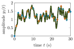
(a) Time simulation.

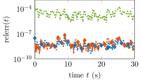
(b) Maximum pointwise relative errors.

Figure 2: Time simulation of the time-delay example: The best reduced-order models from each generating approach are shown. All reduced-order models can recover the system behavior for the given input signal, but the interpolation-based reduced-order models perform around four orders of magnitude better in terms of accuracy than the model generated by POD(avg).

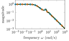
(a) Linear transfer functions.

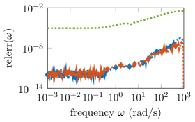
(b) Pointwise relative errors.

Figure 3: Sigma plots showing $\lVert G(\mathfrak{i}\omega))\rVert_{2}$ of the first symmetric subsystem transfer function of the time-delay example: The best reduced-order models from each generating approach are shown. All reduced-order models can recover the system behavior for the given input signal, but the interpolation-based reduced-order models perform around six orders of magnitude better in terms of accuracy than the model generated by POD(avg).

(a) SymInt(VW, avg).

(b) GenInt(VW, avg).

(c) POD(avg).

Figure 4: Second symmetric subsystem transfer function relative approximation errors $\operatorname{relerr}(\omega_{1},\omega_{2})$ of the time-delay example: The best reduced-order models from each generating approach are shown. The errors of both interpolation-based reduced-order models are at least four orders of magnitude better than those of the POD(avg) model.

As first example, we consider the time-delayed heated rod with bilinear feedback from [16, 11], to which we append a quadratic reaction term to obtain

$$\partial_{\mathrm{t}}\nu(\zeta,t) =\Delta\nu(\zeta,t)-2\sin(\zeta)\nu(\zeta,t)+2\sin(\zeta)\nu(\zeta,t-\tau)$$

$$\quad{}-{}2\sin(\zeta)\nu(\zeta,t)^{2}+\sum\limits_{j=1}^{m}b_{j}(\zeta)(\nu(\zeta,t)+1)u_{j}(t),$$

with $(t,\zeta)\in(0,t_{\mathrm{f}})\times(0,\pi)$, boundary conditions $\nu(t,0)=\nu(t,\pi)=0$ for all $t\in[0,t_{\mathrm{f}}]$, and the constant time delay $\tau=1$. After spatial discretization with central finite differences, we obtain a quadratic-bilinear time-delay system of the form

$$E\dot{x}(t) =Ax(t)+A_{\mathrm{d}}x(t-\tau)+H(x(t)\otimes x(t))+\sum\limits_{j=1}^{m}N_{k}x(t)u_{j}(t)+Bu(t),$$

$$y(t) =Cx(t),$$

with $E,A,A_{\mathrm{d}},N_{j}\in\mathbb{R}^{n\times n}$, for $j=1,\ldots,m$, $H\in\mathbb{R}^{n\times n^{2}}$, $B\in\mathbb{R}^{n\times m}$ and $C\in\mathbb{R}^{p\times n}$. For our experiments, we have chosen $n=2\,000$, $m=2$ and $p=2$, where $u_{1}$ controls the temperature of the first third of the rod and $u_{2}$ the rest, and $y_{1}$ observes the temperature of the first half of the rod and $y_{2}$ of the second half. The system has zero initial conditions $x(t)=0$ for all $t\leq 0$.

The reduced-order models are computed as explained in Section 5.1 with a reduced order of $r=24$. In Table 1, we can see that all reduced-order models perform well for this example. However, the interpolation-based models provide smaller errors than those generated by POD, where the better POD model computed by POD(avg) performs mildly worse than the worst interpolation-based reduced-order models. Comparing the different interpolation approaches we can observe that mostly, the interpolation of symmetric transfer functions performs better in the time simulations and in frequency domain than the interpolation of the generalized transfer functions. For the reduced-order models that provide exact interpolation (equi), the sampling of higher-order terms in the generalized transfer function needed to be restricted to match the reduced basis dimension. This restriction is removed in avg such that more information about the bilinear and quadratic terms can be obtained in sampling the generalized transfer functions compared to the symmetric transfer function setting, but this does only lead to a better reduced-order model when measured with $\operatorname{relerr}_{\mathcal{L}_{\infty}}^{(1)}$.

Figure 2 shows the time simulation of the full-order model and the best performing reduced-order models from each method over the time interval $[0,30]$ s. We restricted Figure 2(a) to only the first output signal for clarity, but the pointwise relative errors in Figure 2(b) are computed over both output entries. For the input signals, we have chosen the mean $\mu=2$ and the parameter $\varsigma=0.25$. The interpolation-based methods clearly outperform POD(avg) by approximately four orders of magnitude. There is no significant difference between the errors of SymInt(VW, avg) and GenInt(VW, avg).

Similar results can be observed in frequency domain. The first symmetric subsystem transfer functions are shown in Figure 3, while Figure 4 illustrates the pointwise relative errors of the second symmetric subsystem transfer functions. In both cases, we only show the best performing methods in the frequency interval $\omega,\omega_{1},\omega_{2}\in[10^{-3},10^{3}]$ rad/s. As in the time domain, the interpolation-based methods outperform POD(avg) by several orders of magnitude in terms of accuracy. Further plots of the other methods in time and frequency domain can be found in the accompanying code package [36].

5.3 Particle motion in one-dimensional crystal structures

Table 2: Error table of the Toda lattice example: The errors are computed as shown in Section 5.1. Only the interpolation methods with one-sided projections provide reduced-order models that are stable in the time simulation. The models with $\infty$ error are unstable. SymInt(V, equi) outperforms GenInt(V, equi) by around a factor of $2$.

	$\boldsymbol{\operatorname{relerr}_{L_{2}}}$	$\boldsymbol{\operatorname{relerr}_{L_{\infty}}}$	$\boldsymbol{\operatorname{relerr}_{\mathcal{L}_{\infty}}^{(1)}}$	$\boldsymbol{\operatorname{relerr}_{\mathcal{L}_{\infty}}^{(2)}}$
SymInt(V, equi)	$2.4797\texttt{e-}04$	$4.1415\texttt{e-}04$	$4.5518\texttt{e-}03$	$4.6131\texttt{e-}02$
SymInt(V, avg)	$1.4565\texttt{e-}02$	$1.7264\texttt{e-}02$	$1.4862\texttt{e-}02$	$9.4341\texttt{e-}02$
SymInt(VW, equi)	$\infty$	$\infty$	$3.7049\texttt{e-}03$	$4.4699\texttt{e-}02$
SymInt(VW, avg)	$\infty$	$\infty$	$2.3354\texttt{e-}05$	$2.3035\texttt{e-}01$
GenInt(V, equi)	$5.0036\texttt{e-}04$	$8.4421\texttt{e-}04$	$1.0227\texttt{e-}02$	$5.6204\texttt{e-}02$
GenInt(V, avg)	$4.2052\texttt{e-}03$	$8.5704\texttt{e-}03$	$1.8517\texttt{e-}03$	$2.6190\texttt{e-}02$
GenInt(VW, equi)	$\infty$	$\infty$	$1.3348\texttt{e-}02$	$1.3706\texttt{e+}01$
GenInt(VW, avg)	$\infty$	$\infty$	$8.2451\texttt{e-}06$	$4.5499\texttt{e-}02$
POD	$\infty$	$\infty$	$8.1769\texttt{e-}01$	$7.7696\texttt{e-}01$
POD(avg)	$\infty$	$\infty$	$4.6483\texttt{e-}01$	$6.2382\texttt{e-}01$

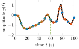
(a) Time simulation.

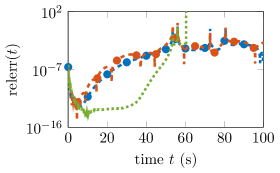
(b) Maximum pointwise relative errors.

Figure 5: Time simulation of the Toda lattice example: The best reduced-order models from each generating approach are shown. Only the interpolation-based reduced-order models recover the system behavior over the full time interval, while POD(avg) becomes unstable after about $60$ s.

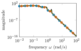
(a) Linear transfer functions.

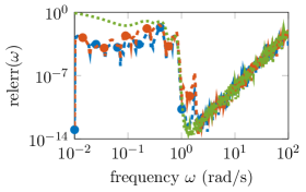
(b) Pointwise relative errors.

Figure 6: First symmetric transfer function of the Toda lattice example: Only the best performing methods from the time simulation are shown. All reduced-order models recover the transfer function behavior of the original system. For low frequencies, POD(avg) performs two order of magnitude worse than the interpolating methods.

(a) SymInt(V, equi).

(b) GenInt(V, equi).

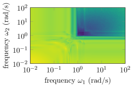
(c) POD(avg).

Figure 7: Second symmetric transfer function relative approximation errors $\operatorname{relerr}(\omega_{1},\omega_{2})$ of the Toda lattice example: Only the best performing methods from the time simulation are shown. For large frequencies, SymInt(V, equi) and POD(avg) perform equally well and better than GenInt(V, equi), while for low frequencies, POD(avg) is an order of magnitude worse than the interpolating methods.

As second example, we consider the motion of particles in a one-dimensional crystal structure described by the Toda lattice model from the introduction; see Figure 1. The original system with exponential nonlinearities Eq. 2 can be rewritten into quadratic-bilinear form by introducing the auxiliary variables

$$z_{j}(t)=\begin{cases}e^{k_{j}(q_{j}(t)-q_{j+1}(t))}-1&\text{for}\leavevmode\nobreak\ j<\ell,\\ e^{k_{\ell}q_{\ell}(t)}-1&\text{for}\leavevmode\nobreak\ j=\ell.\end{cases}$$ (35)

By differentiating Eq. 35 twice, the Toda lattice model can be written as a system of quadratic-bilinear ordinary differential equations of the form

$$0 =M\ddot{q}(t)+D\dot{q}(t)+Kq(t)+H_{\mathrm{vv}}\big{(}\dot{q}(t)\otimes\dot{q}(t)\big{)}+H_{\mathrm{pv}}\big{(}q(t)\otimes\dot{q}(t)\big{)}$$ (36)

$$\quad{}+{}H_{\mathrm{pp}}\big{(}q(t)\otimes q(t)\big{)}-N_{\mathrm{p}}q(t)u(t)-B_{\mathrm{u}}u(t),$$

$$y(t) =C_{\mathrm{v}}\dot{q}(t),$$

with the dimensions as in Eq. 3 and $m=1$ input and $p=1$ output. The exact parameterization of the matrices in Eq. 36 can be found in [35, Sec. 6.5]. For our experiments, we use the same setup as in [35, Sec. 6.5] with $\ell=2\,000$ particles such that Eq. 36 has the order $n=4\,000$.

It has been observed in [35] that the internal block structures of the matrices in Eq. 36 resulting from the original and auxiliary variables should be preserved for stability of the reduced-order models. Therefore, we follow the suggestion in [35, Sec. 6.5] and use the split congruence transformation approach [14, 30, 34]. That is, given a basis matrix $V=\begin{bmatrix}V_{1}^{\mathsf{H}}&V_{2}^{\mathsf{H}}\end{bmatrix}^{\mathsf{H}}\in\mathbb{C}^{2\ell\times r}$, we construct the extended basis matrix

$$\widetilde{V}=\begin{bmatrix}V_{1}&0\\ 0&V_{2}\end{bmatrix}\in\mathbb{C}^{2\ell\times 2r},$$

and similarly for a left basis matrix $W$. The extended basis matrices are then used for model reduction by projection. We apply this approach in our experiments to modify all projection basis matrices computed as described in Section 5.1. By construction, it holds that

$$\operatorname{span}(V)\subseteq\operatorname{span}(\widetilde{V}).$$

Therefore, if $V$ was constructed to satisfy any subspace conditions in Section 4 for interpolation, the basis matrix $\widetilde{V}$ also satisfies these conditions such that interpolation properties are preserved.

For the comparison in our experiments, we have chosen the reduced order of all computed models to be $2r=120$. The results are shown in Table 2. The best performing model in terms of time simulation error is SymInt(V, equi) followed by its counterpart for the generalized transfer functions GenInt(V, equi). None of the models resulting from a two-sided projection has a stable time-domain simulation, which appears to be a consequence of loosing additional mechanical properties by $V\neq W$. Also none of the POD generated models performs stable in the time-domain simulation. Here, the large frequency domain errors indicate that the approximation quality is not sufficient to approximate the system behavior well enough. In frequency domain, we observe similarly to the previous numerical example that SymInt(VW, avg) and GenInt(VW, avg) perform best in terms of approximating the first symmetric subsystem transfer function.

The time-domain simulations of the full- and the best performing reduced-order models from each method are shown in Figure 5 in the time interval $[0,100]$ s. For the input signal, we have chosen the mean $\mu=0$ and the smoothing parameter $\varsigma=2$. POD(avg) performs visibly stable only until around $60$ s, while the other two models follow the system behavior over the complete time interval. The pointwise relative errors in Figure 5(b) reveal POD(avg) to be more accurate than SymInt(V, equi) and GenInt(V, equi) for the first half of the time interval before it assumes the same error level as the other two methods and finally becomes unstable. SymInt(V, equi) and GenInt(V, equi) have overall a similar error behavior, with the errors of GenInt(V, equi) being mildly larger.

On the other hand, in frequency domain, we can observe a similar behavior compared to the previous numerical example. The results for the same reduced-order models that performed best in time domain can be seen in Figures 6 and 7, with the frequency interval of interest $\omega,\omega_{1},\omega_{2}\in[10^{-3},10^{3}]$ rad/s. The POD generated models perform worst, with the exception of GenInt(VW, equi). The models based on oversampling generalized transfer functions perform better than those based on oversampling the symmetric transfer functions due to the additional information obtained from the nonlinear terms. However, in this example we can observe that the oversampling procedure may produce larger errors than exact interpolation. In particular, models computed via avg provide worse approximation errors for larger frequencies, where the transfer functions are converging to zero, while the models with equi preserve the system behavior due to the exact interpolation. Further plots of the other methods in time and frequency domain can be found in the accompanying code package [36].

6 Conclusions

We have extended the structure-preserving interpolation framework to quadratic-bilinear systems. Based on two motivating structured examples, we have introduced the structured variants of the symmetric subsystem and generalized transfer functions of quadratic-bilinear systems. For both transfer function types, we provided subspace conditions enabling the computation of interpolating structured reduced-order models by projection. The theoretical findings are then used to compute structured reduced-order models in two numerical examples. The theory presented here can be applied to a much broader class of structures than those used here for illustrations.

The numerical results suggest that the interpolation of symmetric transfer functions provides more accurate reduced-order models than the generalized transfer functions for the same reduced order. This is most certainly a consequence of the restriction to only products of system terms in the generalized transfer functions. However, we have seen that when the basis matrices are first constructed by oversampling and then compressed, the generalized transfer function interpolation framework provides more accurate reduced-order models for the same computational costs as for the symmetric transfer functions due to additional information obtained from the nonlinear terms. The authors of [17] extend on this oversampling idea and the definition of structured generalized transfer functions for quadratic-bilinear systems from this paper to propose structure-preserving model reduction for systems with polynomial nonlinearities based on the interpolation of generalized transfer functions with at most one nonlinear component. While this gives a first efficient approach to simulation-free model reduction for polynomial systems, there are many open questions left. One related to our observations in this work is the question whether exact interpolation of transfer functions based on Volterra kernels may perform better than an oversampling procedure. This needs a thorough investigation of interpolation conditions for polynomial systems, which we will address in some future work.

Another transfer function type for quadratic-bilinear systems are regular subsystem transfer functions. These have been omitted in this paper since for the choice of identical interpolation points, the projection spaces of regular and symmetric subsystem transfer functions coincide. The formulas for structured variants of regular transfer functions and results on interpolation conditions will be presented in a separate work.

For simplicity of exposition, we have restricted the numerical experiments to only logarithmically equidistant interpolation points on the imaginary axis. While such a procedure is often sufficient in practice, the question of good or even optimal interpolation points remains open and crucial for the success of such model reduction methods. This is still an unresolved issue even in the case of structured linear systems and needs further investigation in the future.

References

- [1] M. I. Ahmad, P. Benner, and I. Jaimoukha. Krylov subspace methods for model reduction of quadratic-bilinear systems. IET Control Theory Appl., 10(16):2010–2018, 2016. doi:10.1049/iet-cta.2016.0415.
- [2] A. C. Antoulas, C. A. Beattie, and S. Gugercin. Interpolatory Methods for Model Reduction. Computational Science & Engineering. SIAM, Philadelphia, PA, 2020. doi:10.1137/1.9781611976083.
- [3] Z. Bai and D. Skoogh. A projection method for model reduction of bilinear dynamical systems. Linear Algebra Appl., 415(2–3):406–425, 2006. doi:10.1016/j.laa.2005.04.032.
- [4] M. Barrault, Y. Maday, N. C. Nguyen, and A. T. Patera. An ‘empirical interpolation’ method: application to efficient reduced-basis discretization of partial differential equations. C. R. Math. Acad. Sci. Paris, 339(9):667–672, 2004. doi:10.1016/j.crma.2004.08.006.
- [5] C. A. Beattie and S. Gugercin. Interpolatory projection methods for structure-preserving model reduction. Syst. Control Lett., 58(3):225–232, 2009. doi:10.1016/j.sysconle.2008.10.016.
- [6] P. Benner and T. Breiten. Two-sided projection methods for nonlinear model order reduction. SIAM J. Sci. Comput., 37(2):B239–B260, 2015. doi:10.1137/14097255X.
- [7] P. Benner and P. Goyal. Balanced truncation model order reduction for quadratic-bilinear control systems. e-print 1705.00160, arXiv, 2017. Optimization and Control (math.OC). doi:10.48550/arXiv.1705.00160.
- [8] P. Benner and P. Goyal. Interpolation-based model order reduction for polynomial systems. SIAM J. Sci. Comput., 43(1):A84–A108, 2021. doi:10.1137/19M1259171.
- [9] P. Benner, P. Goyal, and S. Gugercin. -quasi-optimal model order reduction for quadratic-bilinear control systems. SIAM J. Matrix Anal. Appl., 39(2):983–1032, 2018. doi:10.1137/16M1098280.
- [10] P. Benner, S. Gugercin, and S. W. R. Werner. Structure-preserving interpolation of bilinear control systems. Adv. Comput. Math., 47(3):43, 2021. doi:10.1007/s10444-021-09863-w.
- [11] P. Benner, S. Gugercin, and S. W .R. Werner. A unifying framework for tangential interpolation of structured bilinear control systems. e-print 2206.01657, arXiv, 2022. Numerical Analysis (math.NA). doi:10.48550/arXiv.2206.01657.
- [12] S. Chaturantabut and D. C. Sorensen. Nonlinear model reduction via discrete empirical interpolation. SIAM J. Sci. Comput., 32(5):2737–2764, 2010. doi:10.1137/090766498.
- [13] Z. Drmač and S. Gugercin. A new selection operator for the discrete empirical interpolation method—Improved a priori error bound and extensions. SIAM J. Sci. Comput., 38(2):A631–A648, 2016. doi:10.1137/15M1019271.
- [14] R. W. Freund. Padé-type model reduction of second-order and higher-order linear dynamical systems. In P. Benner, V. Mehrmann, and D. C. Sorensen, editors, Dimension Reduction of Large-Scale Systems, volume 45 of Lect. Notes Comput. Sci. Eng., pages 173–189. Springer, Berlin, Heidelberg, 2005. doi:10.1007/3-540-27909-1_8.
- [15] I. V. Gosea and A. C. Antoulas. Data-driven model order reduction of quadratic-bilinear systems. Numer. Linear Algebra Appl., 25(6):e2200, 2018. doi:10.1002/nla.2200.
- [16] I. V. Gosea, I. Pontes Duff, P. Benner, and A. C. Antoulas. Model order reduction of bilinear time-delay systems. In Proc. of 18th European Control Conference (ECC), pages 2289–2294, 2019. doi:10.23919/ECC.2019.8796085.
- [17] P. Goyal, I. Pontes Duff, and P. Benner. Dominant subspaces of high-fidelity nonlinear structured parametric dynamical systems and model reduction. e-print 2301.09484, arXiv, 2023. Dynamical Systems (math.DS). doi:10.48550/arXiv.2301.09484.
- [18] C. Gu. QLMOR: A projection-based nonlinear model order reduction approach using quadratic-linear representation of nonlinear systems. IEEE Trans. Comput.-Aided Des. Integr. Circuits Syst., 30(9):1307–1320, 2011. doi:10.1109/TCAD.2011.2142184.
- [19] C. Himpe and M. Ohlberger. A unified software framework for empirical Gramians. J. Math., 2013:365909, 2013. doi:10.1155/2013/365909.
- [20] M. Hinze and S. Volkwein. Proper orthogonal decomposition surrogate models for nonlinear dynamical systems: Error estimates and suboptimal control. In P. Benner, V. Mehrmann, and D. C. Sorensen, editors, Dimension Reduction of Large-Scale Systems, volume 45 of Lect. Notes Comput. Sci. Eng., pages 261–306. Springer, Berlin, Heidelberg, 2005. doi:10.1007/3-540-27909-1_10.
- [21] B. Kramer, S. Gugercin, and J. Borggaard. Nonlinear balanced truncation: Part 1 – Computing energy functions. e-print 2209.07645, arXiv, 2022. Optimization and Control (math.OC). doi:10.48550/arXiv.2209.07645.
- [22] B. Kramer and K. E. Willcox. Nonlinear model order reduction via lifting transformations and proper orthogonal decomposition. AIAA J., 57(6):2297–2307, 2019. doi:10.2514/1.J057791.
- [23] K. Kunisch and S. Volkwein. Galerkin proper orthogonal decomposition methods for a general equation in fluid dynamics. SIAM J. Numer. Anal., 40(2):492–515, 2002. doi:10.1137/S0036142900382612.
- [24] S. Lall, J. E. Marsden, and S. Glavaški. Empirical model reduction of controlled nonlinear systems. IFAC Proceedings Volumes (14th IFAC World Congress), 32(2):2598–2603, 1999. doi:10.1016/S1474-6670(17)56442-3.
- [25] D. Lawrence, J. H. Myatt, and R. C. Camphouse. On model reduction via empirical balanced truncation. In Proc. Am. Control Conf., volume 5, pages 3139–3144, 2005. doi:10.1109/ACC.2005.1470454.
- [26] G. P. McCormick. Computability of global solutions to factorable nonconvex programs: Part I — Convex underestimating problems. Math. Program., 10(1):147–175, 1976. doi:10.1007/BF01580665.
- [27] B. Peherstorfer. Model reduction for transport-dominated problems via online adaptive bases and adaptive sampling. SIAM J. Sci. Comput., 42(5):A2803–A2836, 2020. doi:10.1137/19M1257275.
- [28] B. Peherstorfer and K. Willcox. Data-driven operator inference for nonintrusive projection-based model reduction. Comput. Methods Appl. Mech. Eng., 306:196–215, 2016. doi:10.1016/j.cma.2016.03.025.
- [29] E. Qian, B. Kramer, B. Peherstorfer, and K. Willcox. Lift & Learn: Physics-informed machine learning for large-scale nonlinear dynamical systems. Phys. D: Nonlinear Phenom., 406:132401, 2020. doi:10.1016/j.physd.2020.132401.
- [30] T. K. S. Ritschel, F. Weiß, M. Baumann, and S. Grundel. Nonlinear model reduction of dynamical power grid models using quadratization and balanced truncation. at-Automatisierungstechnik, 68(12):1022–1034, 2020. doi:10.1515/auto-2020-0070.
- [31] W. J. Rugh. Nonlinear System Theory: The Volterra/Wiener Approach. The Johns Hopkins University Press, Baltimore, 1981.
- [32] J. M. A. Scherpen. Balancing for nonlinear systems. Syst. Control Lett., 21(2):143–153, 1993. doi:10.1016/0167-6911(93)90117-O.
- [33] M. Toda. Vibration of a chain with nonlinear interaction. J. Phys. Soc. Jpn., 22(2):431–436, 1967. doi:10.1143/JPSJ.22.431.
- [34] A. Van de Walle, F. Naets, E. Deckers, and W. Desmet. Stability-preserving model order reduction for time-domain simulation of vibro-acoustic FE models. Int. J. Numer. Methods Eng., 109(6):889–912, 2017. doi:10.1002/nme.5323.
- [35] S. W. R. Werner. Structure-Preserving Model Reduction for Mechanical Systems. Dissertation, Otto-von-Guericke-Universität, Magdeburg, Germany, 2021. doi:10.25673/38617.
- [36] S. W. R. Werner. Code, data and results for numerical experiments in “Structured interpolation for multivariate transfer functions of quadratic-bilinear systems” (version 1.0), April 2023. doi:10.5281/zenodo.7397069.
- [37] K. Willcox and J. Peraire. Balanced model reduction via the proper orthogonal decomposition. AIAA J., 40(11):2323–2330, 2002. doi:10.2514/2.1570.