Quantum butterfly effect at the crossroads of symmetry breaking

Abstract

We investigate the effect of symmetry breaking on chaos in one-dimensional quantum mechanical models using the numerical chaos diagnostic tool, Out-of-Time-Order Correlator(OTOC). Previous research has primarily shown that OTOC shows exponential growth in the neighbourhood of a local maximum. If this is true, the exponential growth should disappear once the local maximum is removed from the system. However, we find that removing the local maximum by a small symmetry-breaking(perturbation) term to the Hamiltonian does not drastically affect the behaviour of OTOC. Instead, with the increase of perturbation strength, the broken symmetric region expands, causing the exponential growth of OTOC to spread over a broader range of eigenstates. We adopt various potentials and find this behaviour universal. We also use other chaos diagnostic tools, such as Loschmidt Echo(LE) and spectral form factor(SFF), to confirm this. This study confirms that a broken symmetric region is responsible for the exponential growth of the microcanonical and thermal OTOC rather than the local maximum. In other words, OTOC is sensitive to symmetry breaking in the Hamiltonian, which is often synonymous with the butterfly effect.

I Introduction

The Lyapunov exponent, a classical diagnostic tool extensively discussed in [1, 2, 3, 4], effectively characterizes classical chaos by examining the divergence of nearby trajectories in phase space ( a measure of the sensitivity to initial conditions). However, the Heisenberg uncertainty principle dictates that for a system with $N$ degrees of freedom, a single quantum state occupies a volume of $\hbar^{N}$ in classical phase space. Hence, we no longer have the luxury of following individual orbits. Thus, there is a pressing need for a novel chaos diagnostic tool tailored for quantum systems.

Several diagnostic tools are develpoed over the years to detect chaos in quantum systems. Some of them are, level-spacing-distribution[5, 6], SFF[7, 8, 9], level number variance[10, 9, 8], entanglement power[11, 12, 13, 14], quantum coherence[15], Loschmidt echo[16, 17, 18, 19, 20] etc. Nevertheless, one such tool, initially considered in the context of superconductivity[21] rapidly gaining traction in the high energy and condensed matter communities, is the OTOC [22, 23, 24, 25, 26, 27, 28, 29, 30, 31, 32, 33, 34].

The OTOCs, within the framework of quantum mechanics, are the growth of non-commutating quantum mechanical operators describing the Unequal Time Commutation Relations(UTCRs). It is the most potent quantum mechanical analogue of the classical sensitiveness to the initial conditions. However, the OTOC measures sensitivity in a scrambled time order quite differently than its classical counterpart. Unlike classical systems, quantum measurements inherently disturb the measured system, and the OTOCs measure this disturbance by considering both forward and backward time evolution.

In their respective works, several researchers have discussed the behaviour of OTOCs in the context of chaos and potential functions. Hashimoto et al. [35] and R. A. Kidd et al. [36] argued that observing exponential growth in OTOCs near a local maximum of a potential function can be misleading and may not necessarily indicate chaos. Supporting this perspective, Kirkby et al. [37] also claimed that relying solely on OTOCs to detect chaos can yield false signals. Tianrui Xu et al. [38] also argued that the exponential growth of OTOCs, often referred to as scrambling, does not inevitably imply the presence of chaos. In contrast, Takeshi Morita [39] demonstrated that OTOCs for a localized wave packet representing a classical particle near a hill in the potential function exhibit exponential growth.

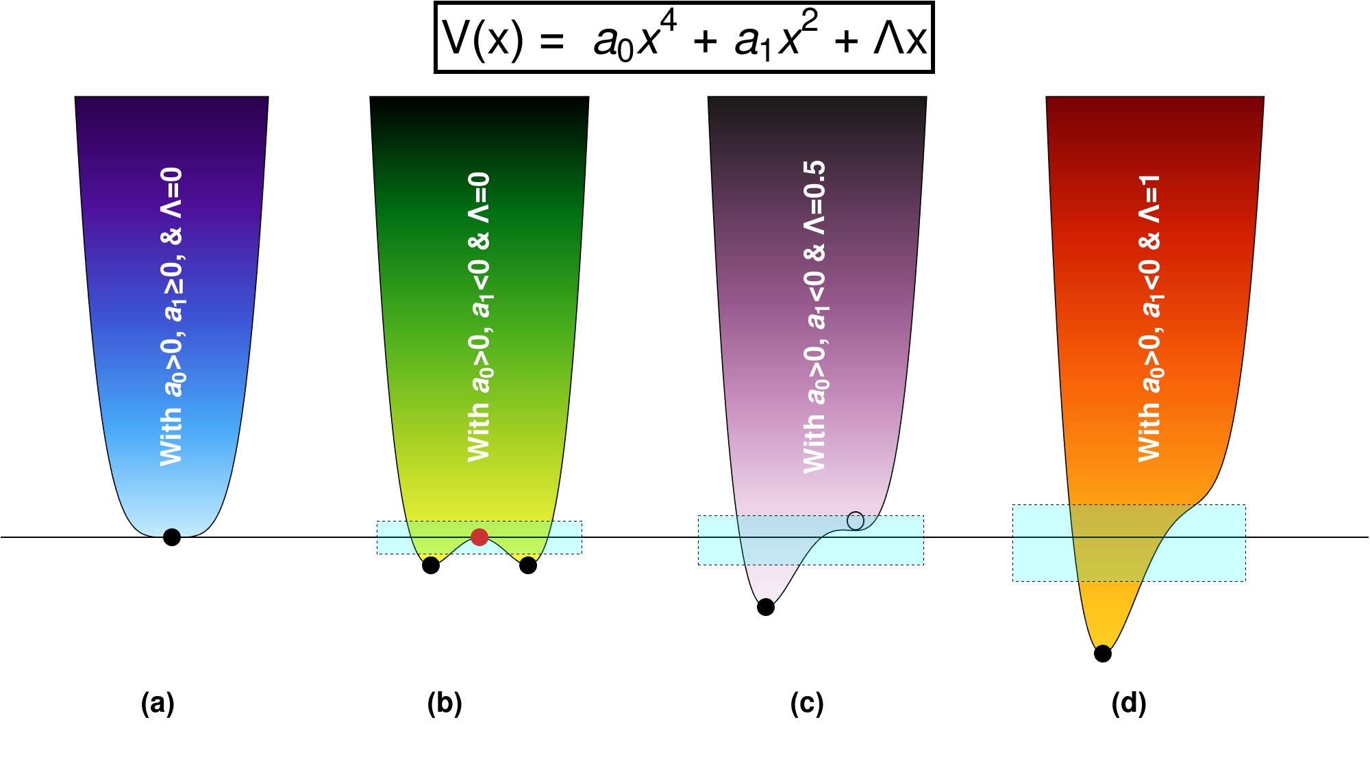
Figure 1: A potential function, $V(x)=a_{0}x^{4}+a_{1}x^{2}+\Lambda x$. (a) $a_{0}>0$, $a_{1}\geq 0$ & $\Lambda=0$, a single well is formed with minimum at $x=0$ having parity symmetry. (b) $a_{0}>0$, $a_{1}<0$, & $\Lambda=0$, the minimum at $x=0$ is now destroyed, giving rise to two symmetrical minima keeping the parity. Such dynamical symmetry breaking follows a pitchfork bifurcation. (c-d) However, for $a_{0}>0$, $a_{1}<0$ & $\Lambda>0$, the symmetry in the double-well is broken explicitly, and the potential landscape becomes asymmetric following a saddle-node bifurcation. Here, $\newmoon\rightarrow$ global minimum, $\newmoon$$\rightarrow$ local maximum, $\fullmoon\rightarrow$ local minimum, and $\blacksquare$$\rightarrow$ broken-symmetric region.

It is important to know, whether removing the saddle point(local maximum) from the potential affects significantly the exponential growth of OTOCs or not. Investigating whether OTOCs continue to exhibit similar behaviour or undergo changes when the saddle point is removed can shed light on the cause of the chaos signature. To explore this, we consider one-dimensional quantum mechanical systems with various polynomial potentials[40, 35, 39, 41, 42, 43, 44] and employ a method of symmetry breaking(SB)[45, 46, 47, 48, 49, 50, 51, 52] by varying a parameter in the system’s potential until the local maximum is eliminated, as shown schematically in Fig.(1). As the saddle point disappears, the potential function becomes asymmetric, driven by a symmetry-breaking term or perturbation. We can also confirm this asymmetry in the Hamiltonian by looking at the eigenstate structure[46]. The previously almost degenerate eigenstates, in the symmetric potential well, split and become non-degenerate in that asymmetry potential well by an amount almost equal to the asymmetry term. Our primary aim is to measure the effect of asymmetry on OTOC, whether enhancing or suppressing the exponential growth or spreading it over a larger neighbourhood as the asymmetry strength(the overall perturbation) increases. We reconfirmed the signature of chaos by measuring Loschmidt Echo and Spectral Form Factor(SFF) for all the models under nearly identical scenarios.

This paper is organised as follows. In section( II), we discuss the formalism to compute the OTOC for a quantum mechanical system with time-independent Hamiltonian. In section( III), we devise three models, namely $Model(I)$, a double well, $Model(II)$, a triple well and $Model(III)$, a double well with a plateau. In this section, we also discuss the solution to the Schrödinger equations of these quantum mechanical models under different perturbation strengths and show the energy distributions. By adding perturbation, we break the primitive symmetry present in these systems and force them to devolve into asymmetric states. In section( IV), we measure the effect of symmetry breaking by measuring microcanonical and thermal OTOCs. Section( V) contains a detailed analysis of our numerical observations including Loschmidt echo and SFF. Finally, in section( VI), we summarise our results and make a few closing remarks.

II OTOC in quantum mechanics for a time-independent Hamiltonian

A 2N-point OTOC [23, 28] is defined as:

$$C_{\beta}(t_{1},t_{2})=-\expectationvalue{\commutator{\hat{x}(t_{1})}{\hat{p}(t_{2})}^{N}}$$ (1)

While the $N=1$ case exhibits random but decaying behaviour, studying the $N=2$ case, involving the four-point correlator, provides a complete understanding of time disorder averaging. Exploring higher-order cases would be unnecessary for our study.

For simplicity, we take $t_{1}=t$ and $t_{2}=0$ in Eq.(1), and define the four-point OTOC[53] as:

$$\mathcal{C}_{\beta}(t)=-\expectationvalue{\commutator{\hat{x}(t)}{\hat{p}}^{2}}$$ (2)

where, $\beta=\dfrac{1}{k_{B}T}$, also known as “the coldness function”, $\hat{x}$ and $\hat{p}$ are respectively quantum mechanical operators for position and momentum.

Using the classical-quantum correspondence[54, 55], $\dfrac{[,]}{i\hbar}\rightarrow\{,\}_{poisson}$, one can show its subtle relation with the classical Lyapunov exponent as follows,

$$\begin{array}[]{r@{}l}\frac{1}{i\hbar}\expectationvalue{[x(t),p(0)]}&\rightarrow\{x(t),p(0)\}=\partialderivative{x(t)}{x(0)}\sim e^{\lambda_{L}t}\\ -\frac{1}{\hbar^{2}}\expectationvalue{[x(t),p(0)]^{2}}&\rightarrow\{x(t),p(0)\}^{2}=\quantity(\partialderivative{x(t)}{x(0)})^{2}\sim e^{2\lambda_{L}t}\end{array}$$ (3)

Thus, from the above semi-classical connection, OTOC quantifies the sensitivity of time evolutions in both chaotic and non-chaotic quantum systems to their initial conditions. In non-chaotic systems, fluctuations exhibit periodic, aperiodic, or irregular behaviour, whereas, in the case of chaotic quantum systems, the random time disordering phenomenon is characterized by exponential growth[56, 57, 58, 59, 60, 61]. Here, we assume that the classical-quantum correspondence can break down after the Ehrenfest time, making it more challenging to detect exponential developments in quantum systems compared to classical ones[62].

For a natural Hamiltonian with the form,

$$\mathcal{H}=\sum_{i=1}^{N}\dfrac{p_{i}^{2}}{2}+\mathcal{U}(x_{1},x_{2},...,x_{N}),$$ (4)

and partition function,

$$Z(\beta)=\sum{e^{-\beta\mathcal{H}}}=\sum_{m}{e^{-\beta E_{m}}}$$ (5)

eq.(2) takes the form [40, 35, 56, 63, 64],

$${}\mathcal{C}_{\beta}(t)=\dfrac{1}{Z(\beta)}\sum_{m}e^{-\beta E_{m}}c_{m}(t)$$ (6)

where, $H\ket{m}=E_{m}\ket{m}$ and

$${}c_{m}(t)=\dfrac{1}{4}\sum_{k,l,r}x_{ml}~{}x_{lk}~{}x_{rm}~{}x_{kr}\bigglb(E_{rk}~{}E_{lk}e^{itE_{rl}}+E_{mr}~{}E_{ml}e^{-itE_{rl}}-E_{rk}~{}E_{ml}e^{it(E_{rm}+E_{lk})}-E_{mr}~{}E_{lk}e^{-it(E_{rm}+E_{lk})}\bigglb)$$ (7)

We refer $c_{m}(t)$, in Eq.(7), for a fixed energy eigenstate as Microcanonical OTOC and $\mathcal{C}_{\beta}(t)$, in Eq.(6), as a Thermal OTOC. Here, $E_{nm}=E_{n}-E_{m}$, $x_{nm}=\matrixelement{n}{\hat{x}}{m}$ and $p_{nm}=\matrixelement{n}{\hat{p}}{m}$.

III Models

The Hamiltonian of the harmonic oscillator(HO) is given by,

$$H=\dfrac{\hat{p}^{2}}{2~{}m}+\dfrac{m~{}\omega^{2}}{2}\hat{x}^{2}$$ (8)

Here, we work in the natural units( $\hbar=1$) and, without any loss of generality, we assume that the mass of the oscillator, $m=1$. Depending on the value of frequency $\omega$, three different cases arise: for real positive value, we have a harmonic oscillator potential; for zero, we have a free particle and for imaginary number, we have an inverted harmonic oscillator(IHO)[42, 65, 66, 67, 68, 69, 70, 71, 72]. In this work, we will be mainly concerned with the Hamiltonians having an inverted harmonic oscillator term.

The inverted quantum oscillator, a physically realized system, exhibits an unstable point at (x=0, p=0) in phase space. When perturbed, the particle undergoes exponential acceleration away from this fixed point, resulting in divergent solutions in phase space. We have taken different manifestations of the IHO in our study, denoted as $Model(I)$ (III.1), and $Model(III)$ (III.3), each having distinct forms of lower bounds and hilltops. Furthermore, $Model(II)$ (III.2) notably employs the HO potential form to create a triple-well configuration.

III.1 $Model(I)$: Double Well

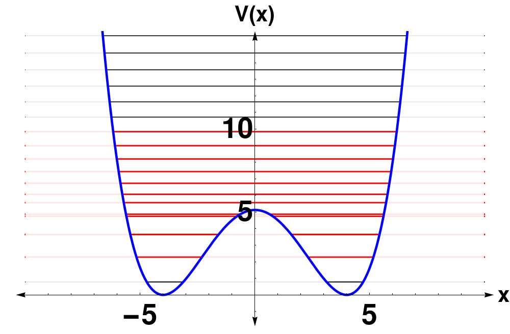
(a) Model(I) Potential.

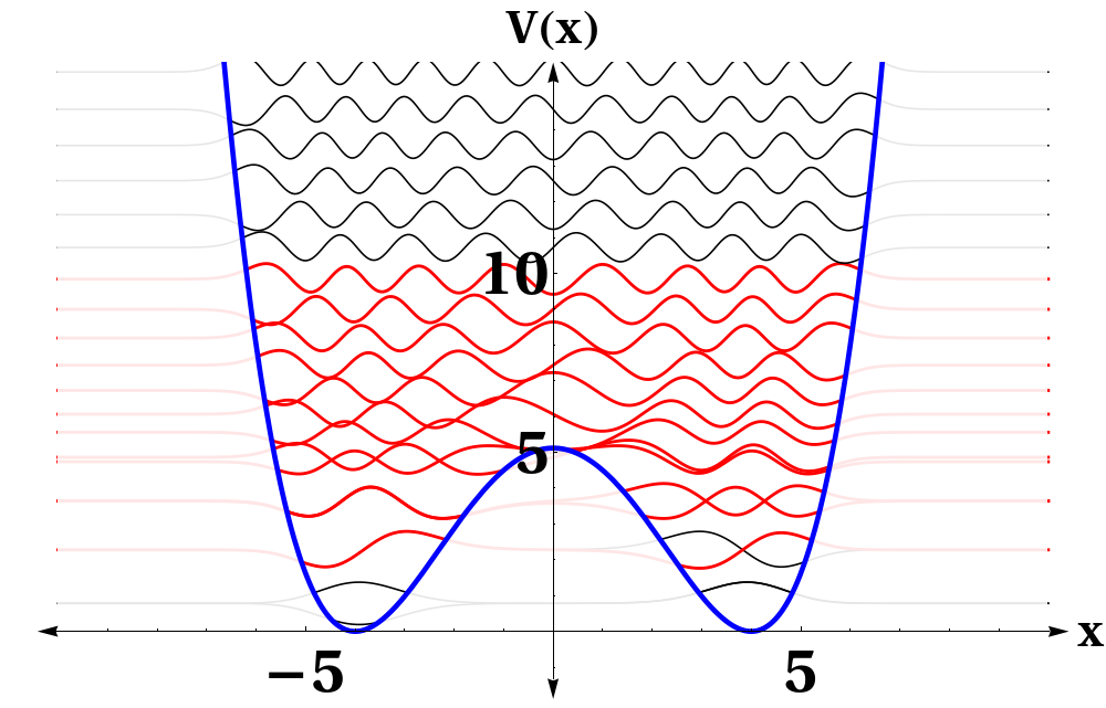
(b) Model(I) Energy Eigenfunctions.

Figure 2: Potential shape and energy eigenvalues for $Model(I)$ with $a_{0}=0.02$, $a_{1}=0.64$ and $\sigma=0.0$. The energy levels below the top of the hill are non-degenerated, and the red lines near the hilltop of the potential show exponential growth in OTOC.

Let us consider, a Hamiltonian of the form of:

$$\mathcal{H}=\frac{-1}{2}\laplacian_{x}+V(x)$$ (9)

here, for $Model(I)$, $V(x)$ is in the form of a non-linear potential function:

$$V(x) = a_{0}~{}\hat{x}^{4}-a_{1}~{}\hat{x}^{2}+\quantity(\sigma~{}\sqrt{\frac{a_{0}}{2~{}a_{1}}})~{}\hat{x}$$ (10a)

$$\Rightarrow V(x) = a_{0}~{}\hat{x}^{4}-a_{1}~{}\hat{x}^{2}+~{}\Lambda\;\hat{x}$$ (10b)

where, $a_{0}$, $a_{1}$ and $\sigma$ are known as stabilisation, destabilisation and asymmetry parameter, respectively. Note that the term $x^{4}$ provides a lower bound to the potential, and here it is taken to be zero for all the models. The parameter $\Lambda$ stands for the perturbation strength.

It is evident in this constructed system that the non-degenerate energy doublets have a splitting $\Delta=\sigma$, i.e. splitting between levels remains close to $\sigma$ for all doublets lying below the barrier top. The initial inspiration for devising the model is taken from [73, 74, 75, 76].

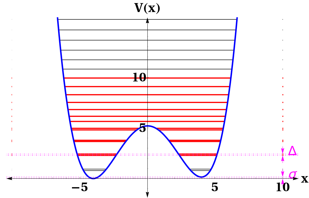
(a) $\sigma=0.15$

(b) $\sigma=10.0$

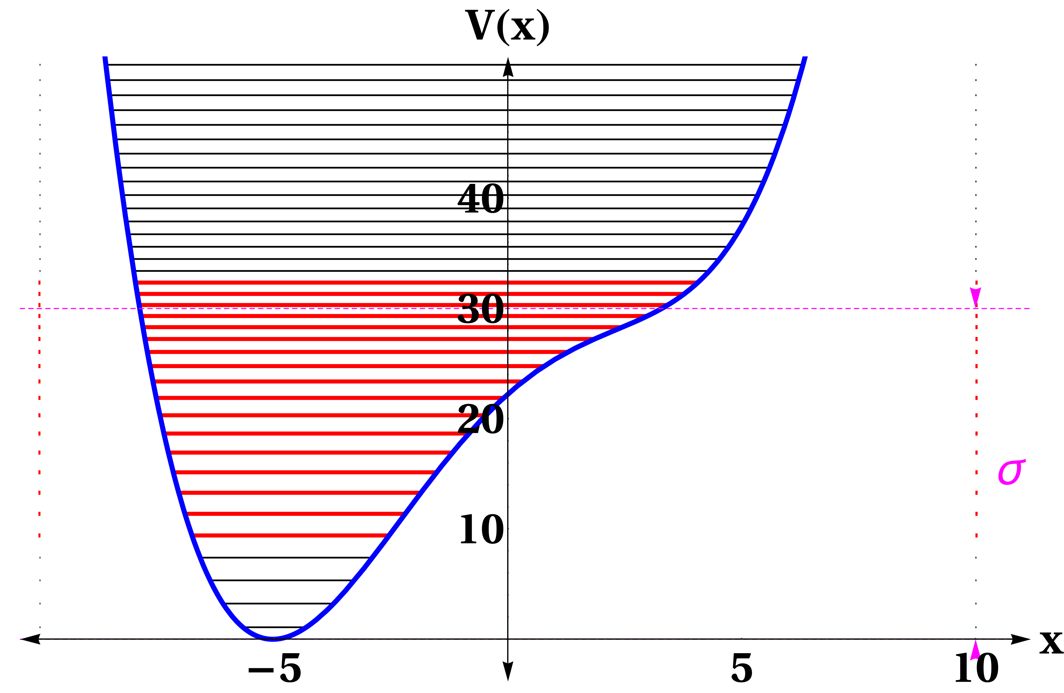
(c) $\sigma=30.0$

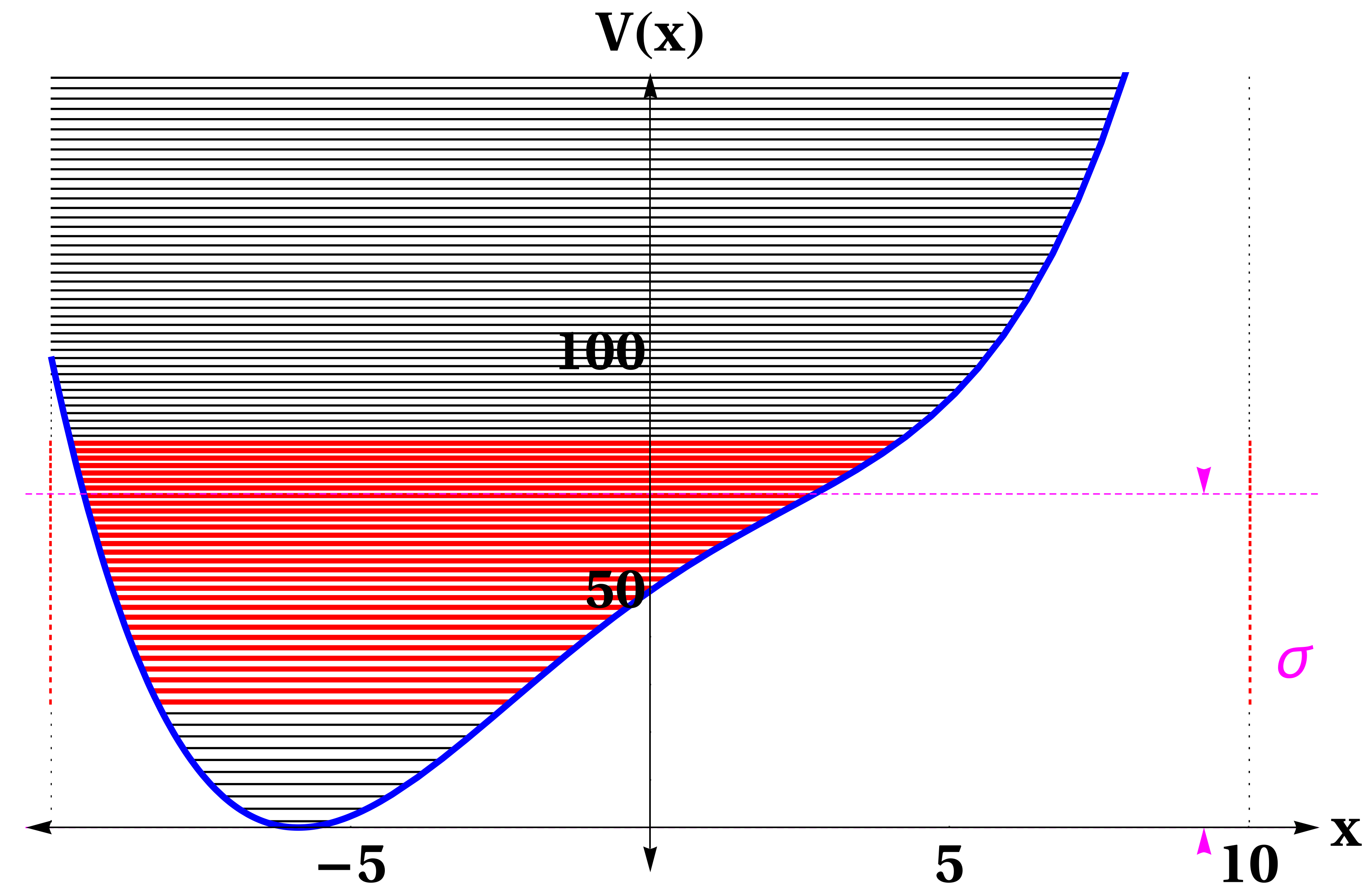
(d) $\sigma=70.0$

Figure 3: $Model(I)$ with different values of $\sigma$.

We numerically solve the time-independent Schrödinger equation considering the Hamiltonian in Eq.(9) in Mathematica 12.0 using NDEigensystem built-in command and obtain the energy eigenvalues $E_{n}$ and the wave functions $\psi_{n}(x)$ for all the models. The results for $Model(I)$ with $\sigma=0$ are shown in Fig.(2). Here, the eigenstates below the hilltop are non-degenerate even though the Hamiltonian and the potential are symmetric under space inversion[77, 78, 79]. Fig.(3) shows the energy eigenvalues for $\sigma$ having values $0.15$, $10.0$, $30.0$ and $70.0$ for $Model(I)$.

All our numerical observations on $Model(I)$ and $Model(III)$ are carried out by considering the width ($\Delta L$) to be 20, $L$ ranging from -10 to 10. Below $\Delta L=15$, the energy separation between levels proliferates, causing the calculation of thermal OTOC very challenging. However, for $Model(II)$, since it contains harmonic terms, so $\Delta L$ could range from $-\infty$ to $\infty$.

III.2 $Model(II)$ : Triple Well

Triple-well potentials have applications in various areas of physics, such as the study of molecular dynamics, where they can be used to model the behaviour of molecules in a triple-well potential energy landscape. They also have possible applications in quantum computing, where they can be used as a building block for quantum gates and algorithms.

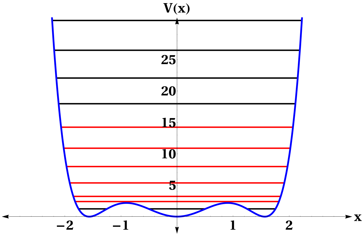
(a) $\sigma=0.0$

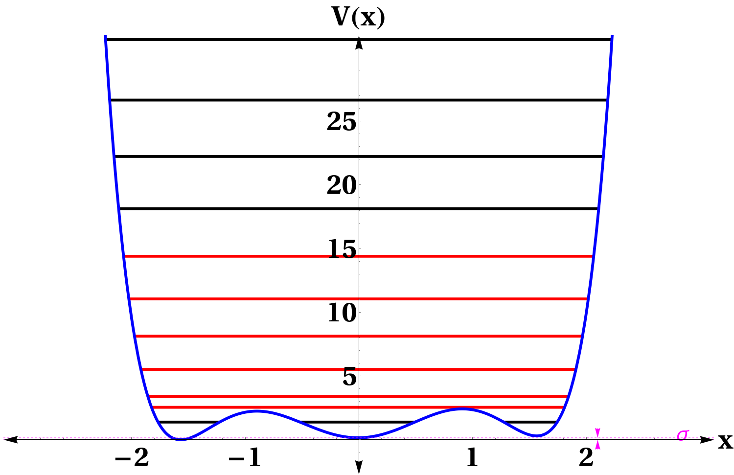
(b) $\sigma=0.15$

(c) $\sigma=10.0$

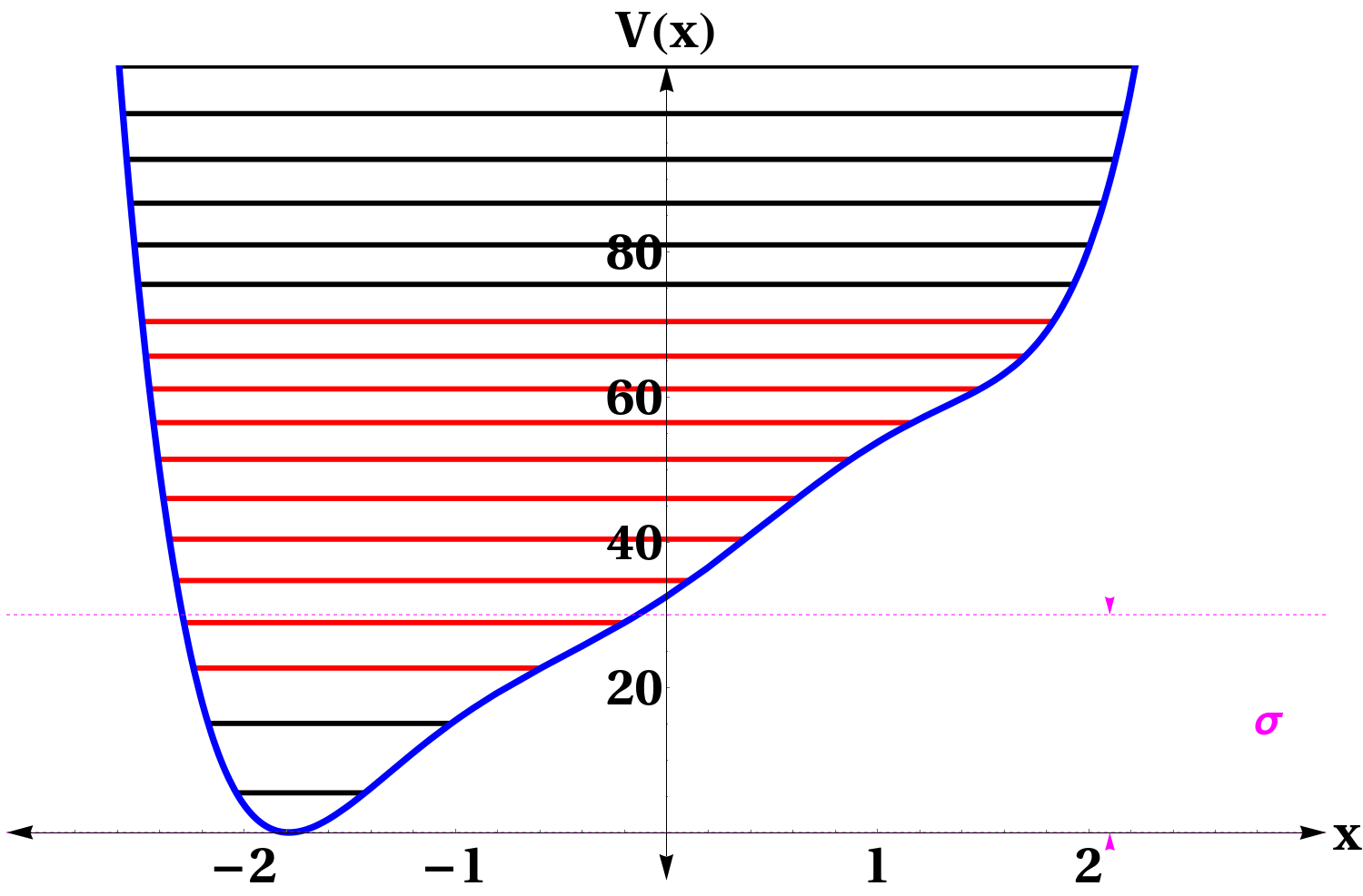
(d) $\sigma=30.0$

Figure 4: $Model(II)$ with different values of $\sigma$.

This model is primarily inspired by the work on [42, 43, 44]. The potential in Eq. (9) for this case is

$$V(x)=a_{1}~{}x^{2}-a_{0}~{}x^{4}+x^{6}+\Lambda~{}x$$ (11)

where $m=1$, $a_{0}=4.9$, $a_{1}=6$.

Fig.(4) shows the potential structure and the corresponding energy eigenvalue distributions under different values of $\sigma$.

III.3 $Model(III)$ : Double Well With A Plateau

The double-well potential[39, 41] with perturbation has a modified version:

$$V(x)=a_{0}~{}\hat{x}^{6}-a_{1}~{}\hat{x}^{4}+\Lambda~{}\hat{x}$$ (12)

where $a_{0}~{}=\frac{1}{142}$, $a_{1}~{}=0.15$, $x^{4}$ produces a plateau instead of a hilltop and $x^{6}$ term gives a lower bound to the potential.

The double-well potential arises in various contexts in physics, including in the study of condensed matter systems, such as in modelling phase transitions and superconductors’ behaviour. It is also used to model the behaviour of a particle in a symmetric potential energy landscape. The energy barrier between the two wells in $Model(I)$ is relatively low and narrow. However, in this model, barrier is broader and taller for which quantum particles are more likely to become trapped in one of the wells.

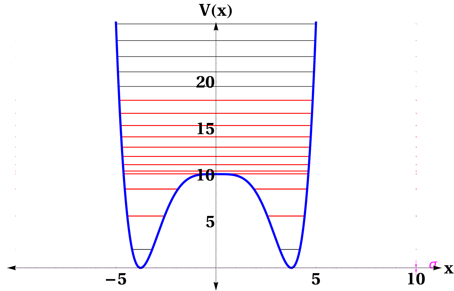
(a) $\sigma=0.0$

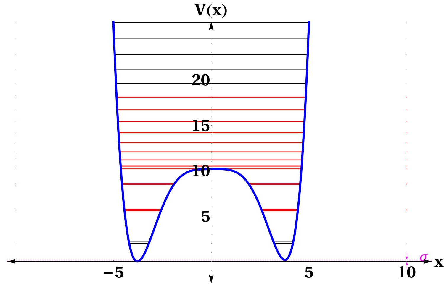
(b) $\sigma=0.15$

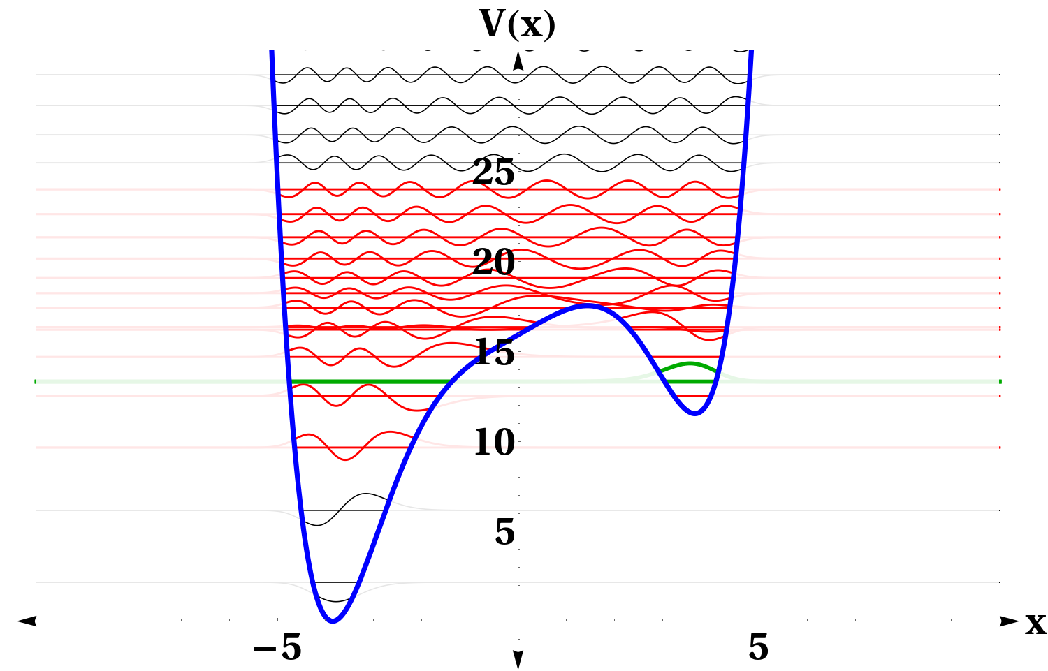
(c) $\sigma=10.0$

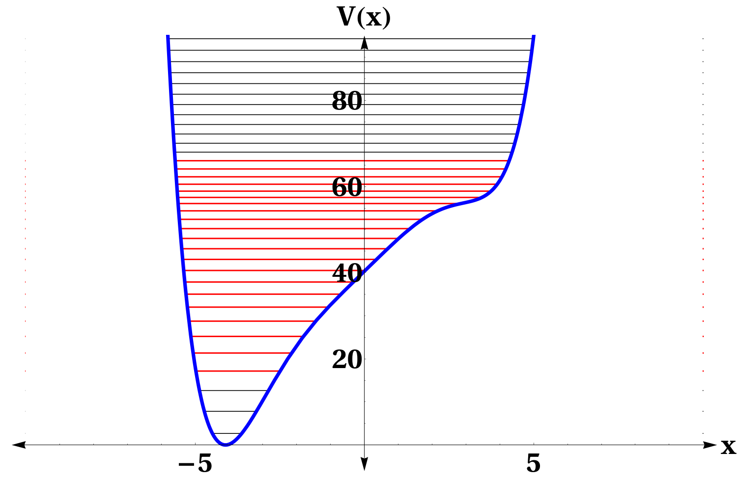
(d) $\sigma=50.0$

Figure 5: $Model(III)$ with different values of $\sigma$.

In Fig.(5), we depict the potential structure and corresponding energy eigenvalues for $\sigma=0.0$, $0.15$, $10.0$, and $50.0$. Notably, as the asymmetry strength increases, degeneracy vanishes from the system, leading the plateau to transition into a local maximum at $\sigma=0.15$ and $10.0$. At $\sigma=50$, the local maximum or plateau disappear entirely. This phenomenon emerges by introducing varying levels of asymmetry strength, thereby breaking the system’s symmetry.

IV Result

In this section, we numerically observe OTOC for several values of perturbation strengths. In other words, we measure the effect of symmetry breaking on the behaviour of OTOC. The exponential growth for microcanonical OTOCs is shown in red colour in all three models. All calculations are performed using a time-step of $0.1$ for computational efficiency and steadfast convergence.

IV.1 Model(I)

Consistent with previous result[35], at $\sigma=0$, microcanonical OTOC for $Model(I)$ display exponential growth within a small energy eigenfunction range(from $n=4$ to $15$) around the local maximum of the potential, highlighted in red in Fig.(6(a)). Similarly, in Fig.(6(b)), the thermal OTOC exhibit exponential growth at higher temperatures.

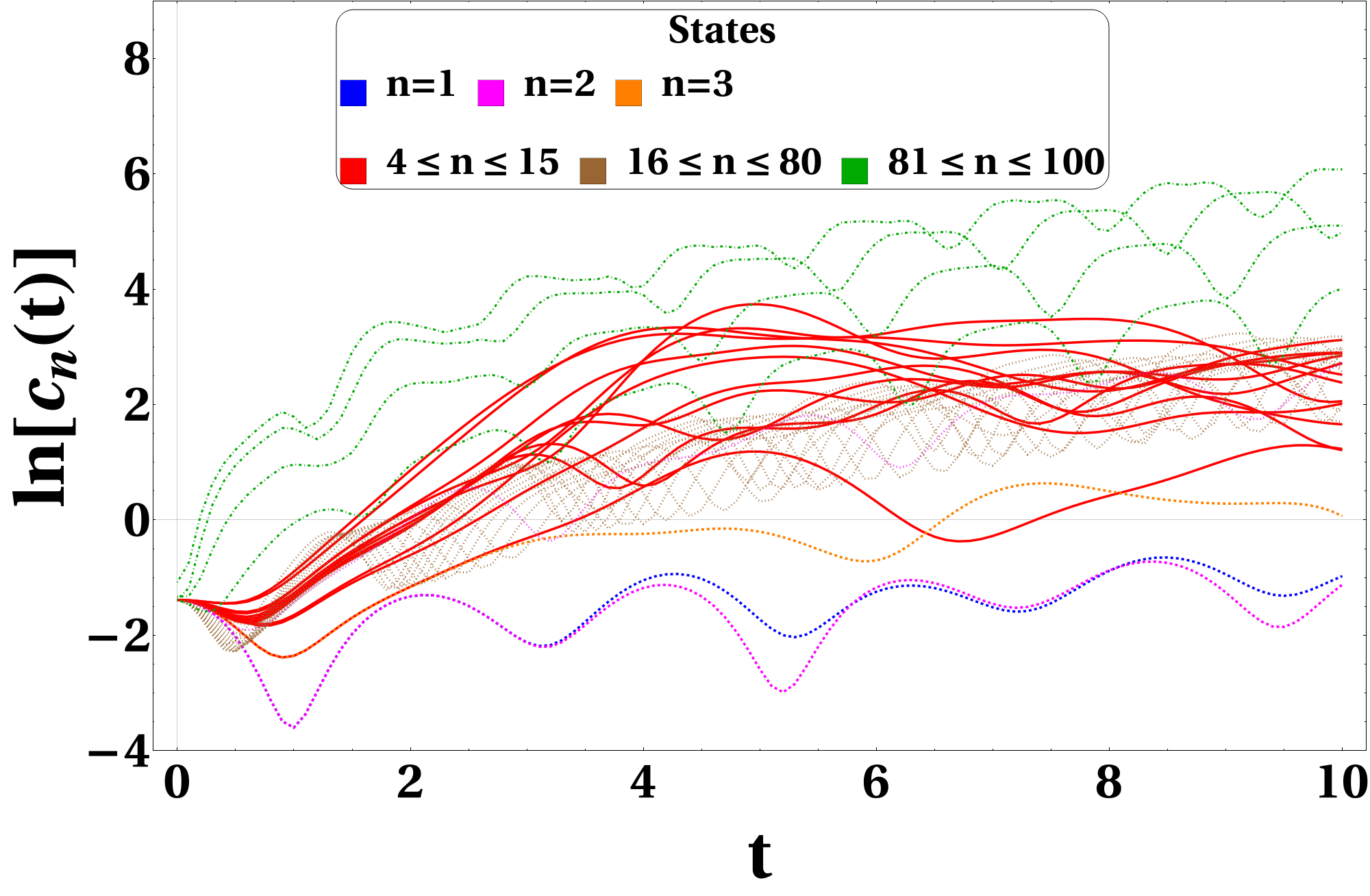
(a) Microcanonical OTOC

(b) Thermal OTOC

Figure 6: OTOCs for $Model(I)$ with $\sigma=0.0$.

Additionally, Figs.(7), (8), (9), and (10) depict OTOC behaviour for $\sigma$ values of $0.15$, $10$, $30$, and $70$ respectively.

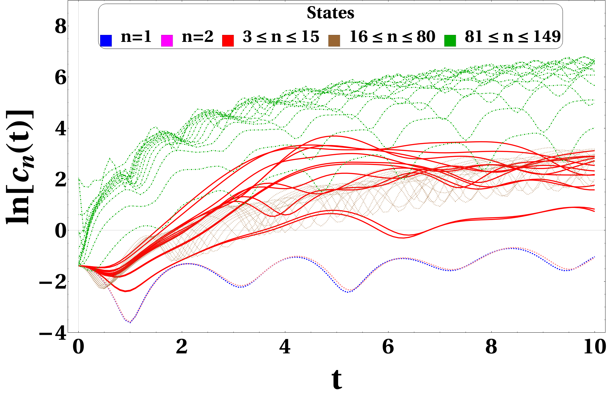
(a) Microcanonical OTOC

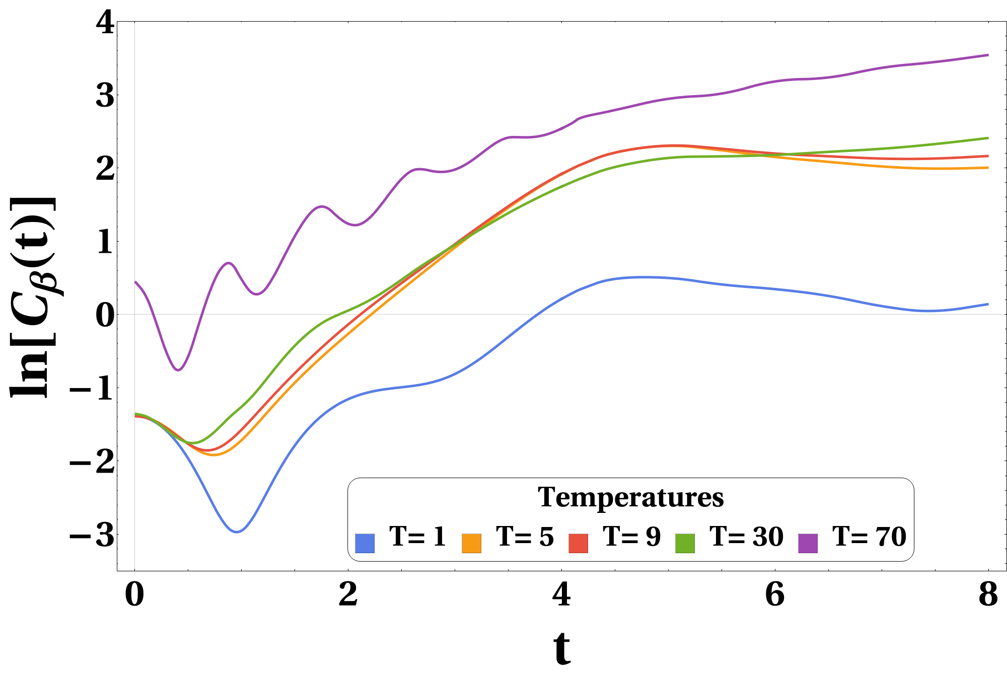
(b) Thermal OTOC

Figure 7: OTOCs of Model(I) with $\sigma=0.15$.

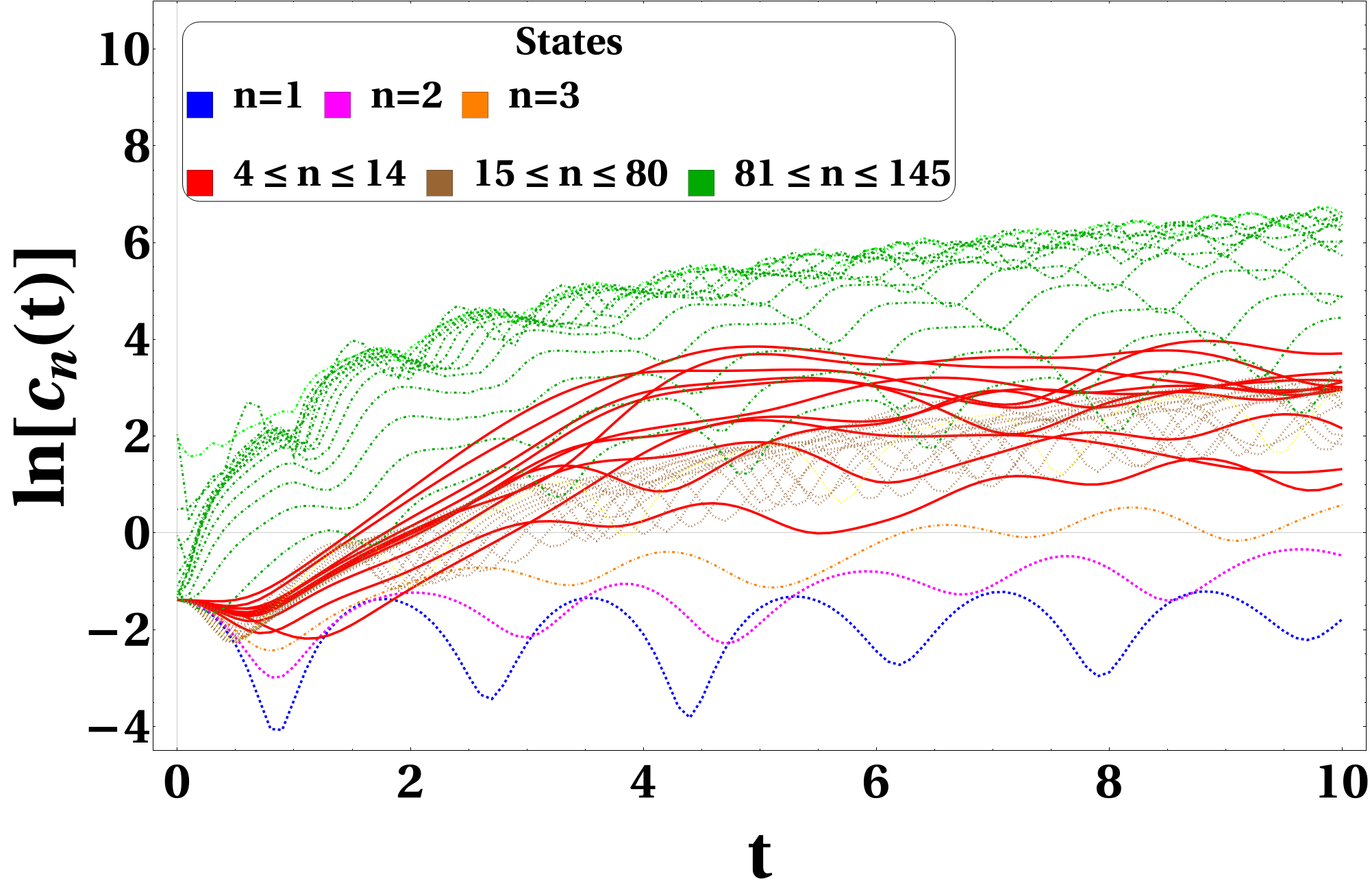
(a) Microcanonical OTOC

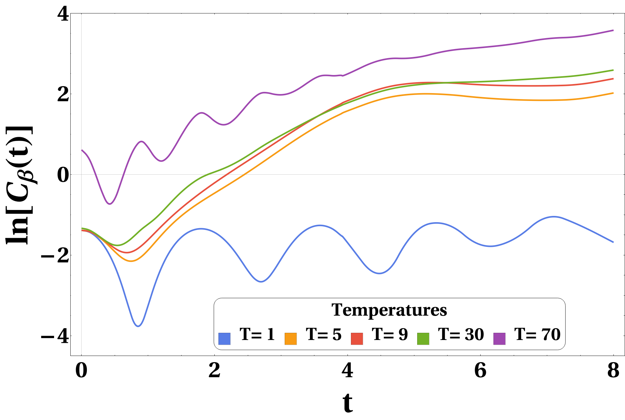
(b) Thermal OTOC

Figure 8: OTOCs of $Model(I)$ with $\sigma=10.0$.

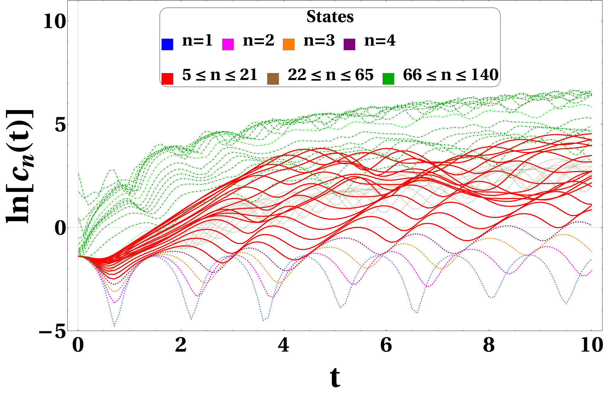
(a) Microcanonical OTOC

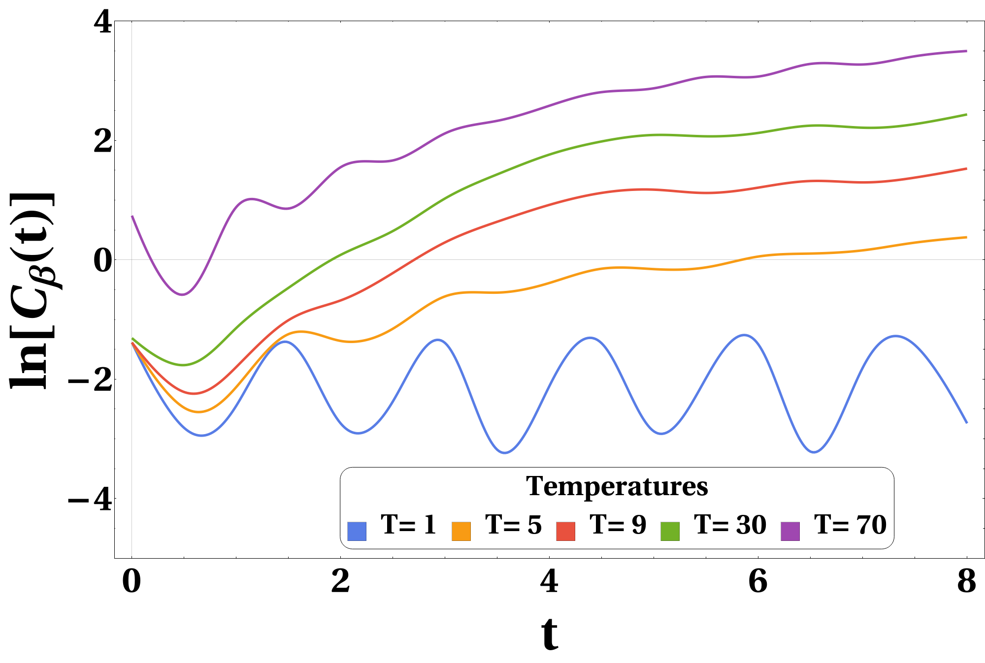
(b) Thermal OTOC

Figure 9: OTOCs for $Model(I)$ with $\sigma=30.0$.

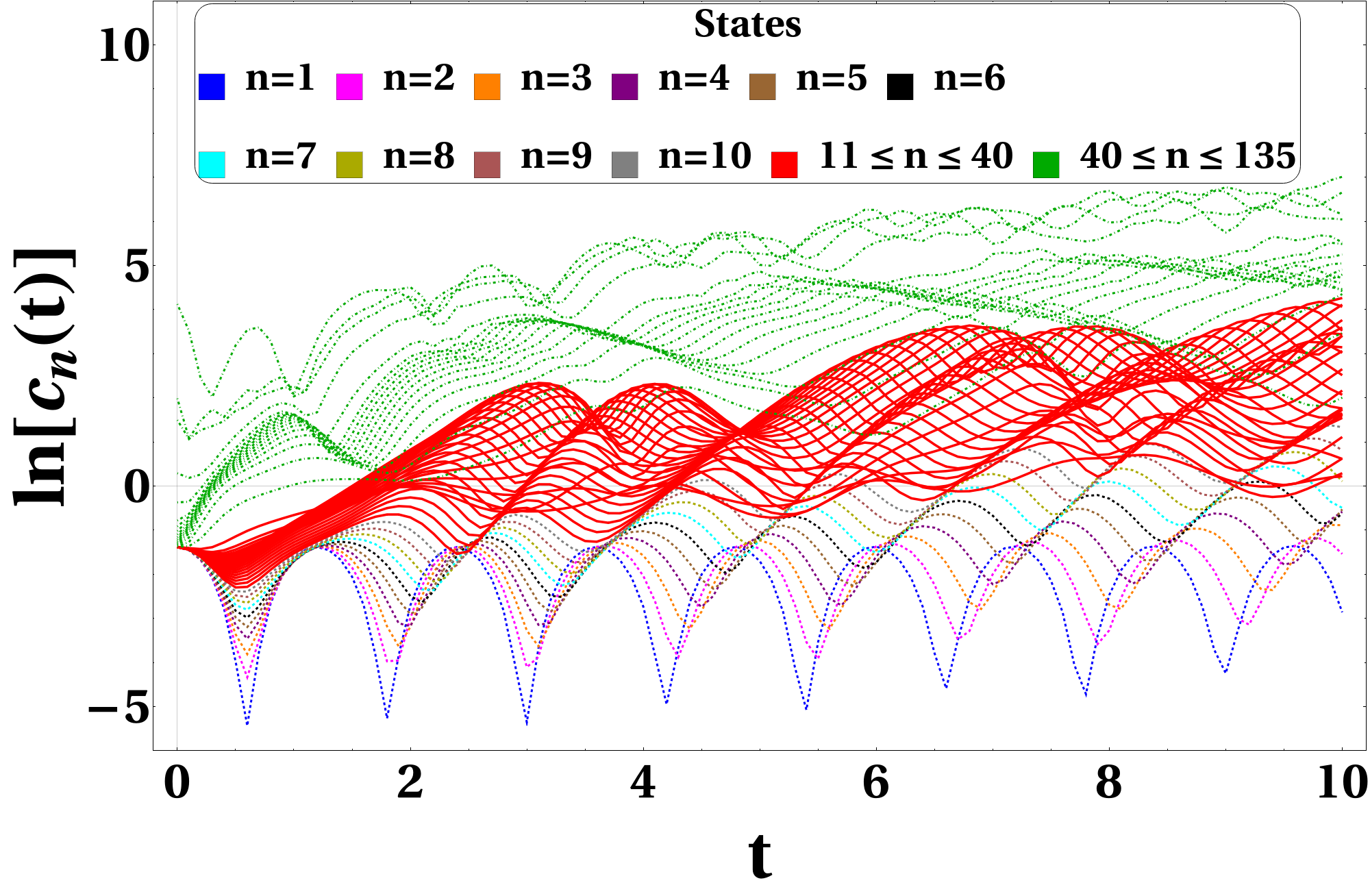
(a) Microcanonical OTOC

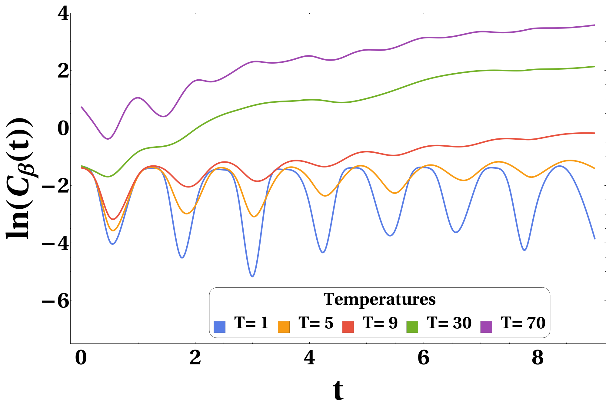
(b) Thermal OTOC

Figure 10: OTOCs for $Model(I)$ with $\sigma=70.0$.

Like the previous result, the exponential growth of OTOCs is observed in Figs.(7) and (8) for $\sigma=0.15$ and $10.0$, respectively, around the hilltop of the potential. It is to notice here that with the increase of the asymmetry parameter($\sigma$), the broken symmetric region expands and with that, the number of states showing exponential growth also widens.

Furthermore, in Fig.(3(c)), $\sigma=30.0$ leads to the disappearance of the local maximum in the potential, yet both microcanonical and thermal OTOCs display sustained exponential growth (Fig.(9)) within the Ehrenfest time. Here, the number of energy levels that show exponential growth have significantly increased from $n=5$ to $n=21$ with the increase in the broken symmetry region. For $\sigma=70.0$ (Fig.(3(d))), the potential lacks a local maximum entirely, but a broader energy levels spectrum still exhibit exponential growth in microcanonical OTOC (Fig.(10)), albeit with the shortest growth duration. However, in this case, the thermal OTOC shows no such growth.

IV.2 Model(II)

In Figs.(11(a)) and (11(b)), microcanonical OTOC exhibits exponential growth around the peaks of the potential for $\sigma=0.0$ and $0.15$ respectively, in the range from $n=2$ to $n=7$. Similarly, thermal OTOC at higher temperatures also displays exponential growth for the same $\sigma$ values, as illustrated in Figs.(12(a)) and (12(b)).

In Fig.(4(c)), at $\sigma=10.0$, the local maximum disappears in the potential, causing the broken symmetry region to expand. In this extended region, both microcanonical and thermal OTOCs continue their exponential growth, as depicted in Figs.(11(c)) and (12(c)).

At $\sigma=30.0$, in Fig.(4(d)), the potential completely lacks a local maximum, resulting in a broader broken symmetric region. Consequently, a more sweeping range of energy levels continues to manifest exponential growth, albeit with a shorter duration, as shown in Figs.(11(d)) and (12(d)). However, at this specific value of $\sigma$, the thermal OTOC exhibits random aperiodic behaviour.

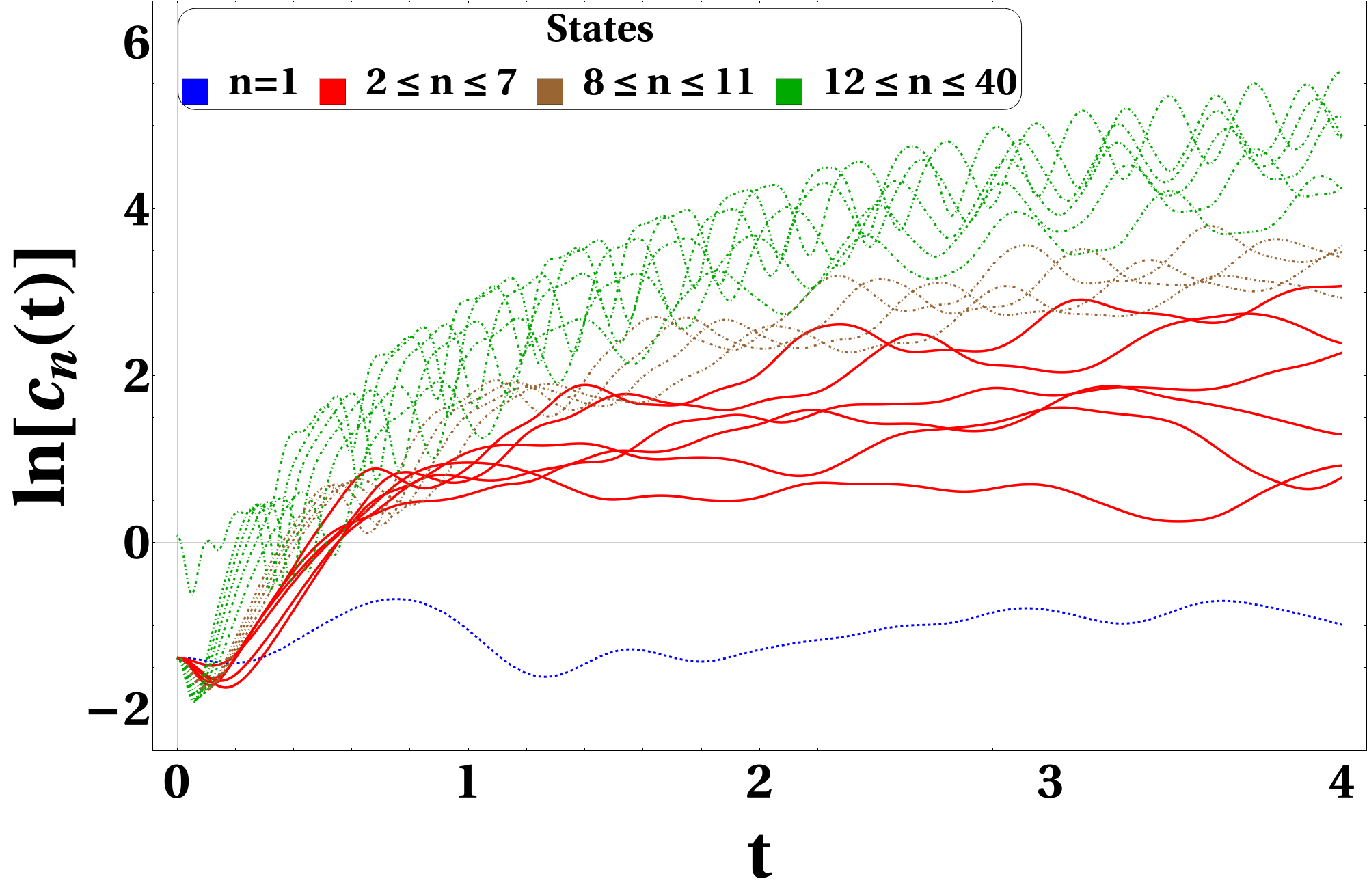
(a) $\sigma=0.0$

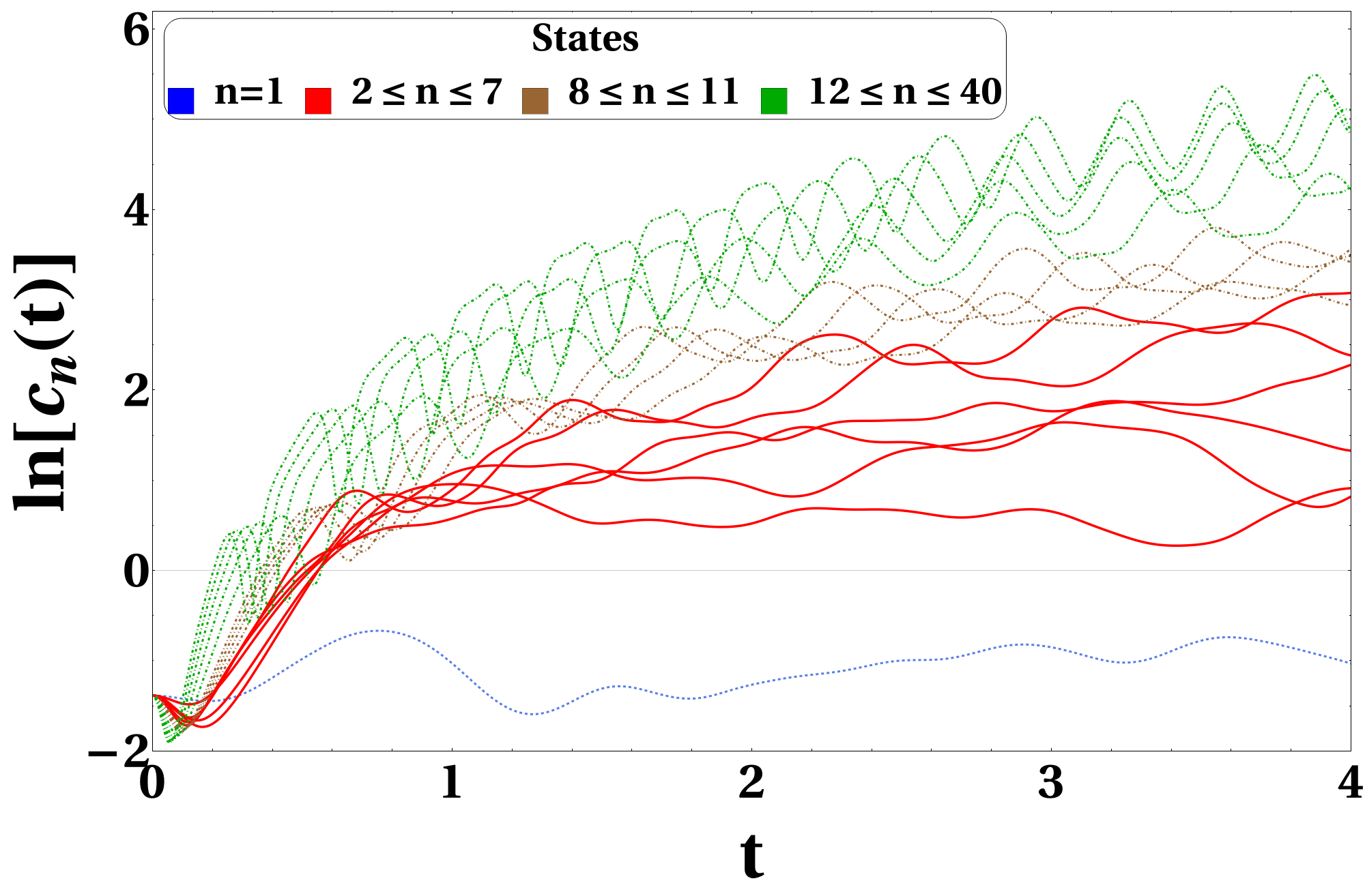
(b) $\sigma=0.15$

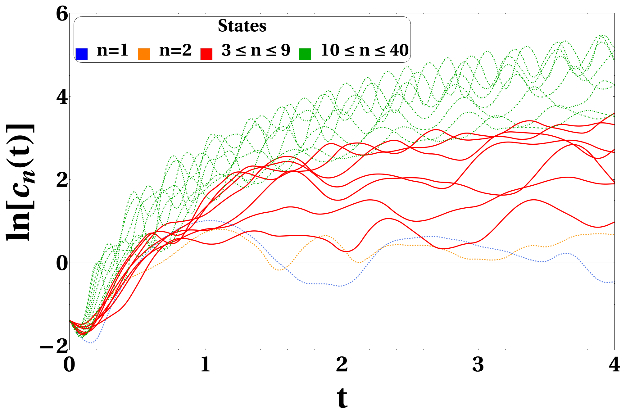
(c) $\sigma=10.0$

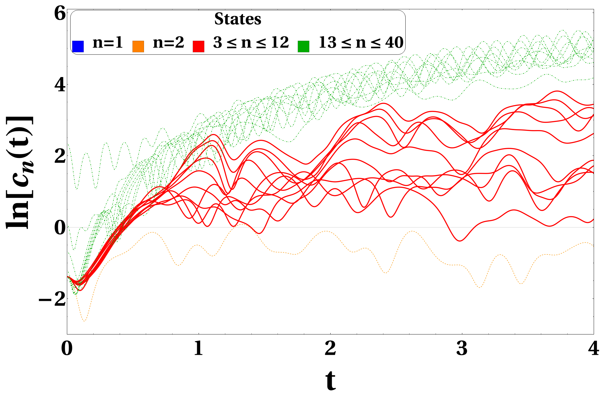
(d) $\sigma=30.0$

Figure 11: Microcanonical OTOCs for $Model(II)$, at different values of $\sigma$.

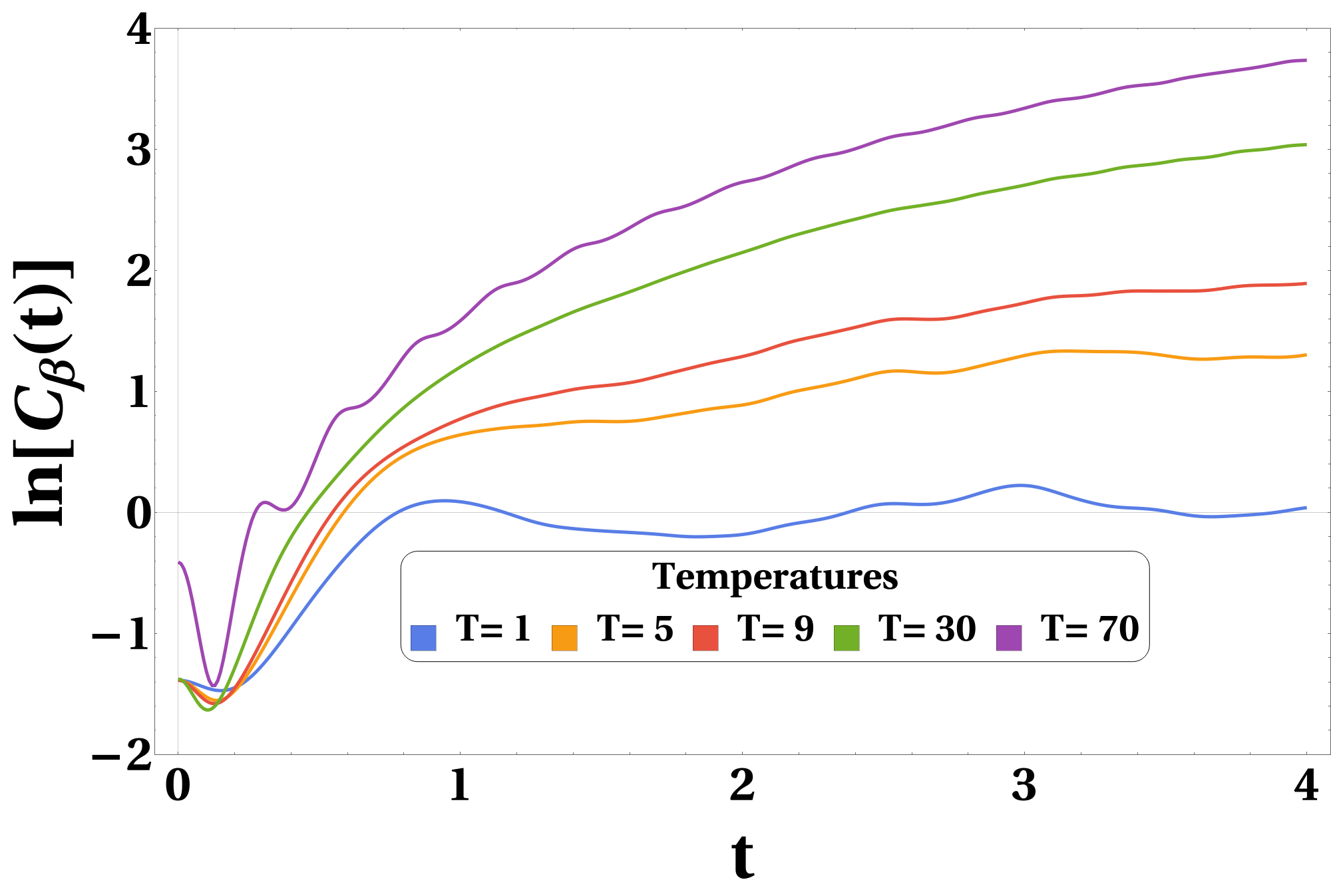
(a) $\sigma=0.0$

(b) $\sigma=0.15$

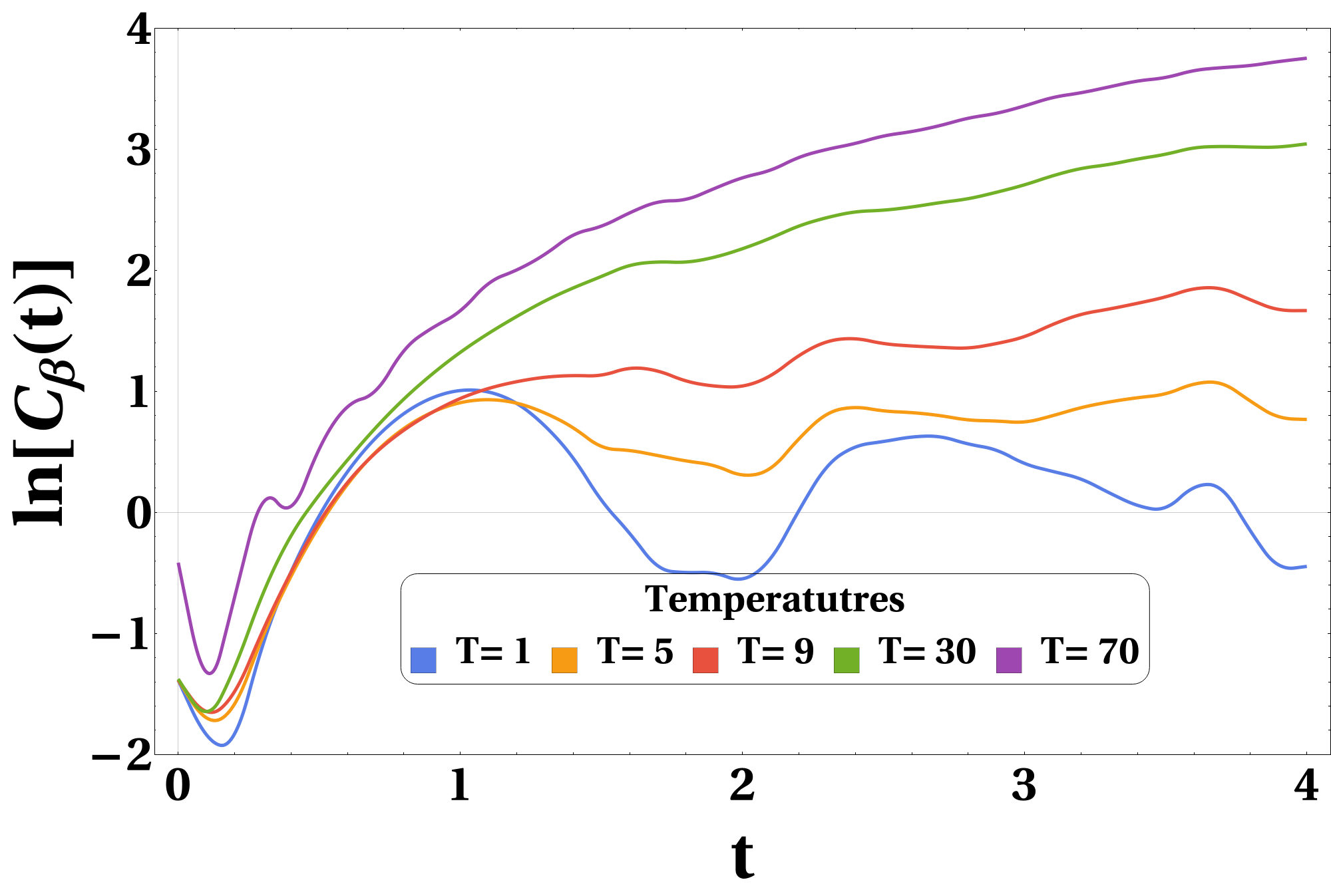
(c) $\sigma=10.0$

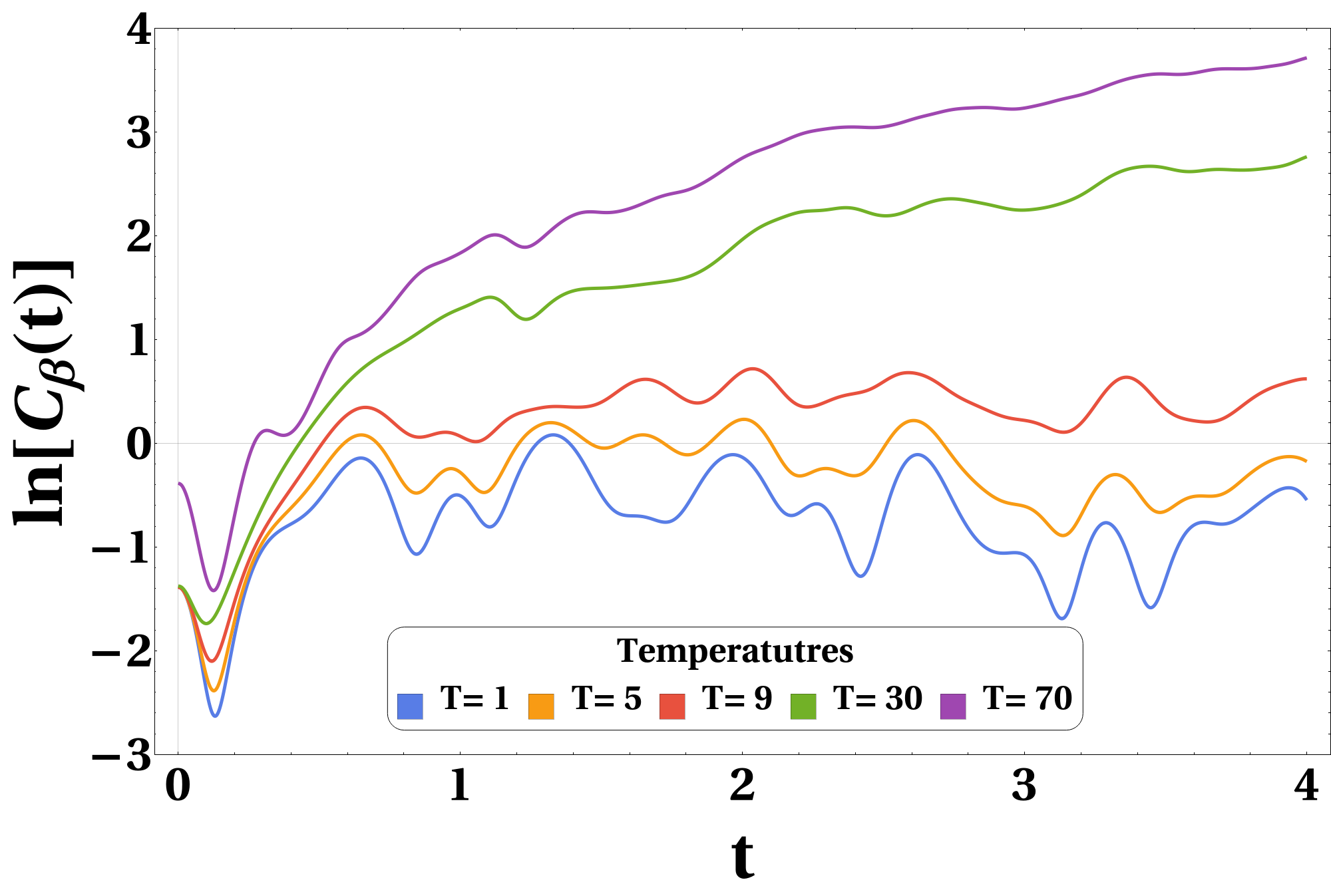
(d) $\sigma=30.0$

Figure 12: Thermal OTOCs for $Model(II)$ at different values of $\sigma$.

IV.3 Model(III)

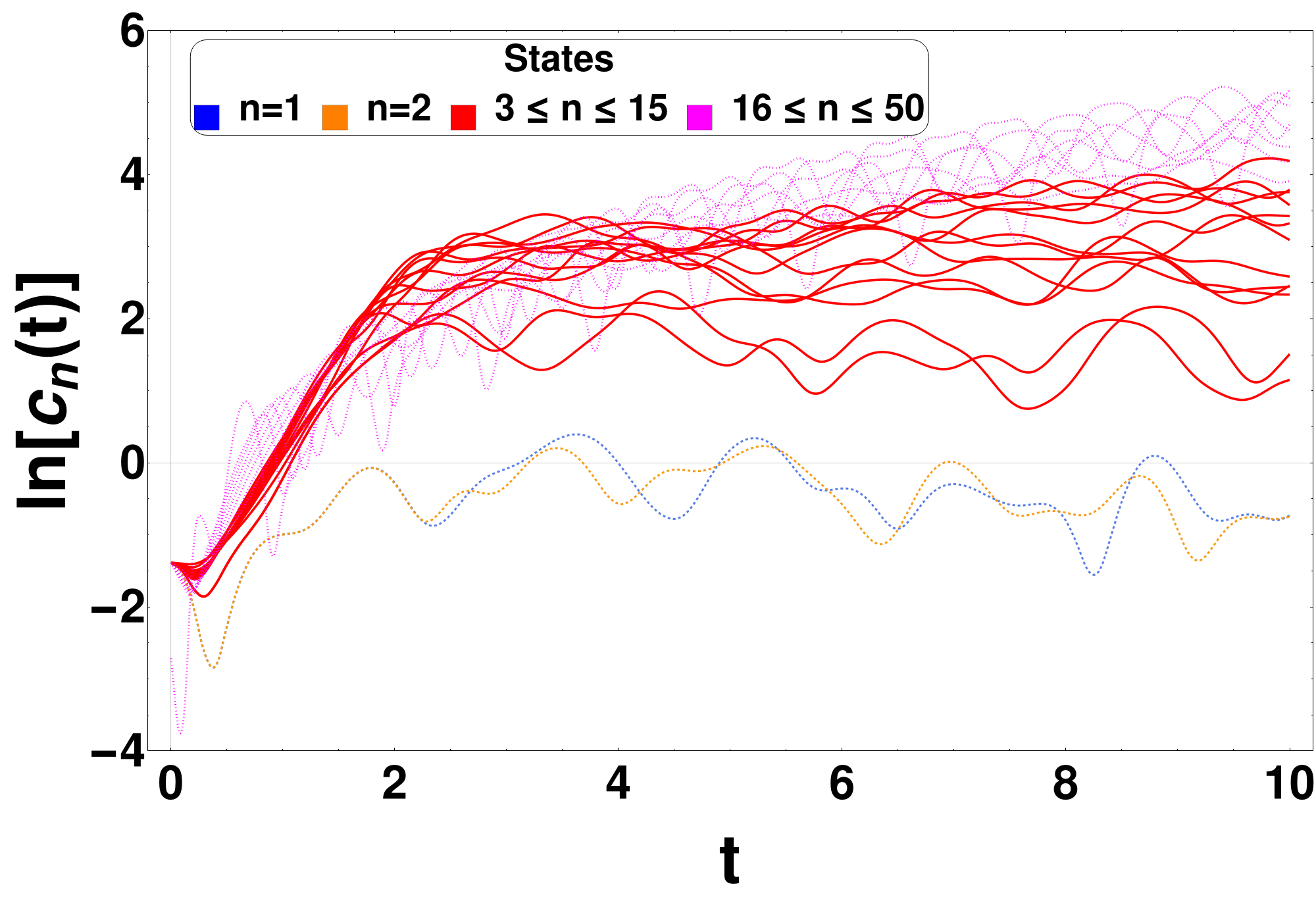
(a) $\sigma=0.0$

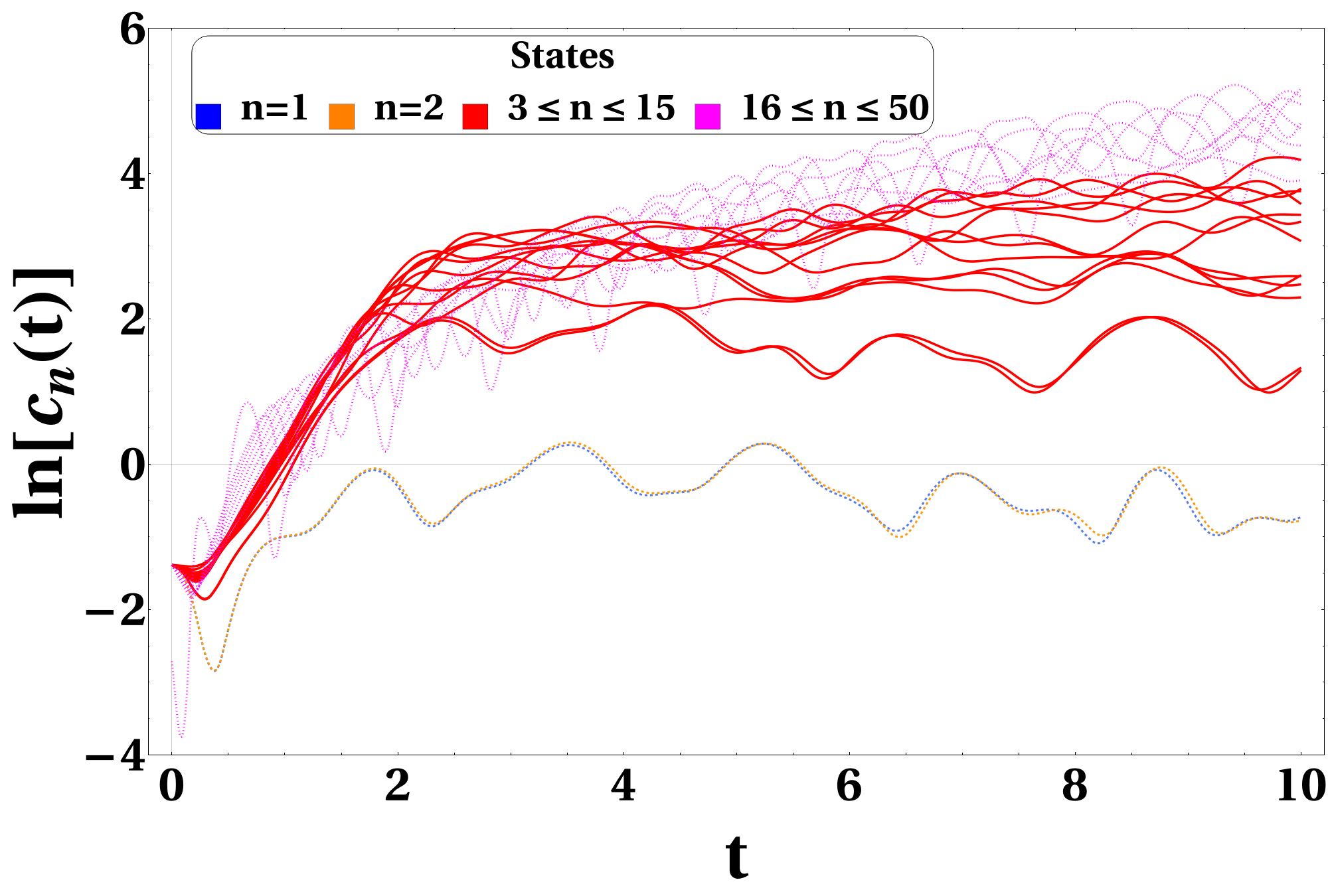
(b) $\sigma=0.15$

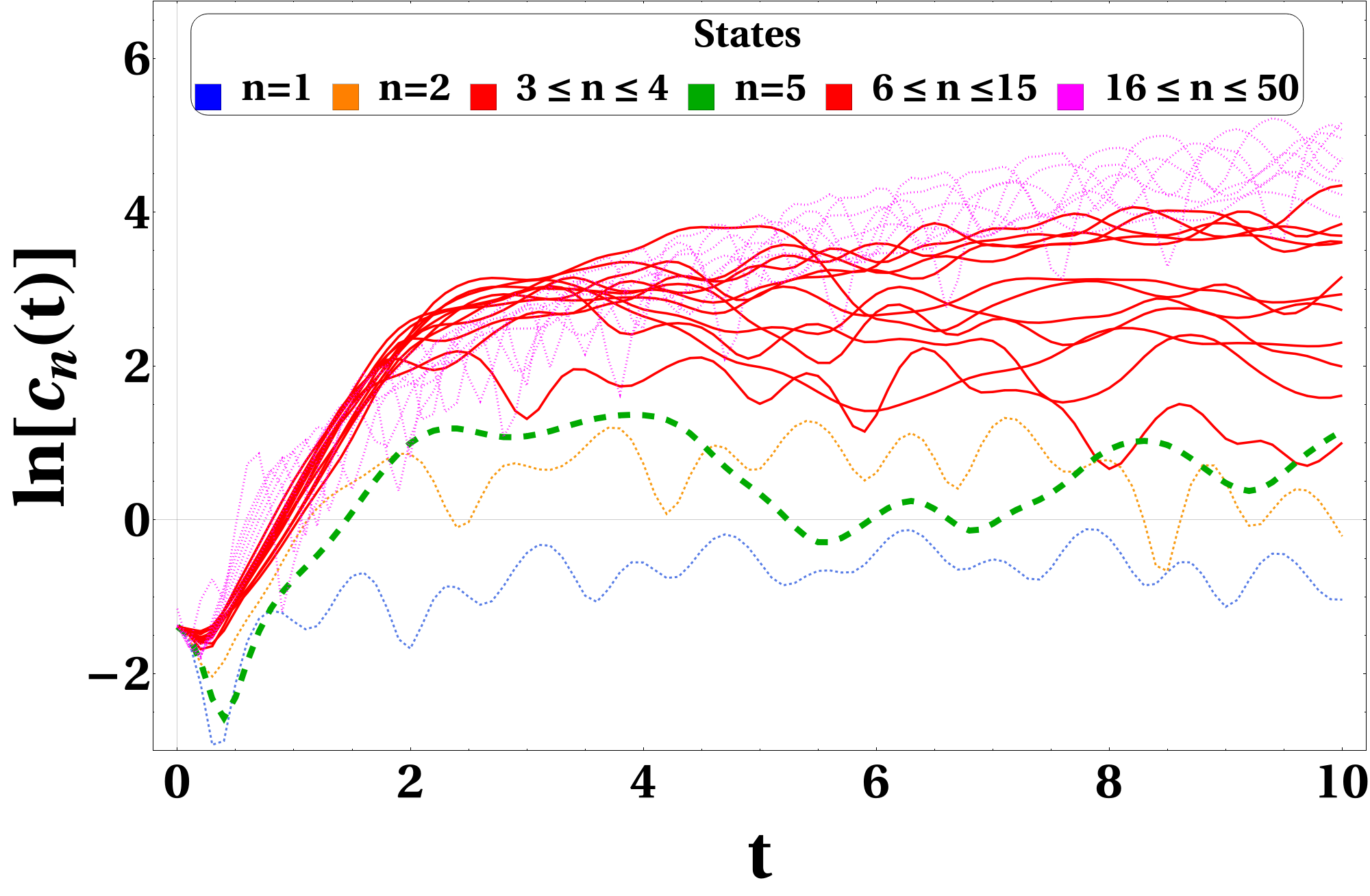
(c) $\sigma=10.0$

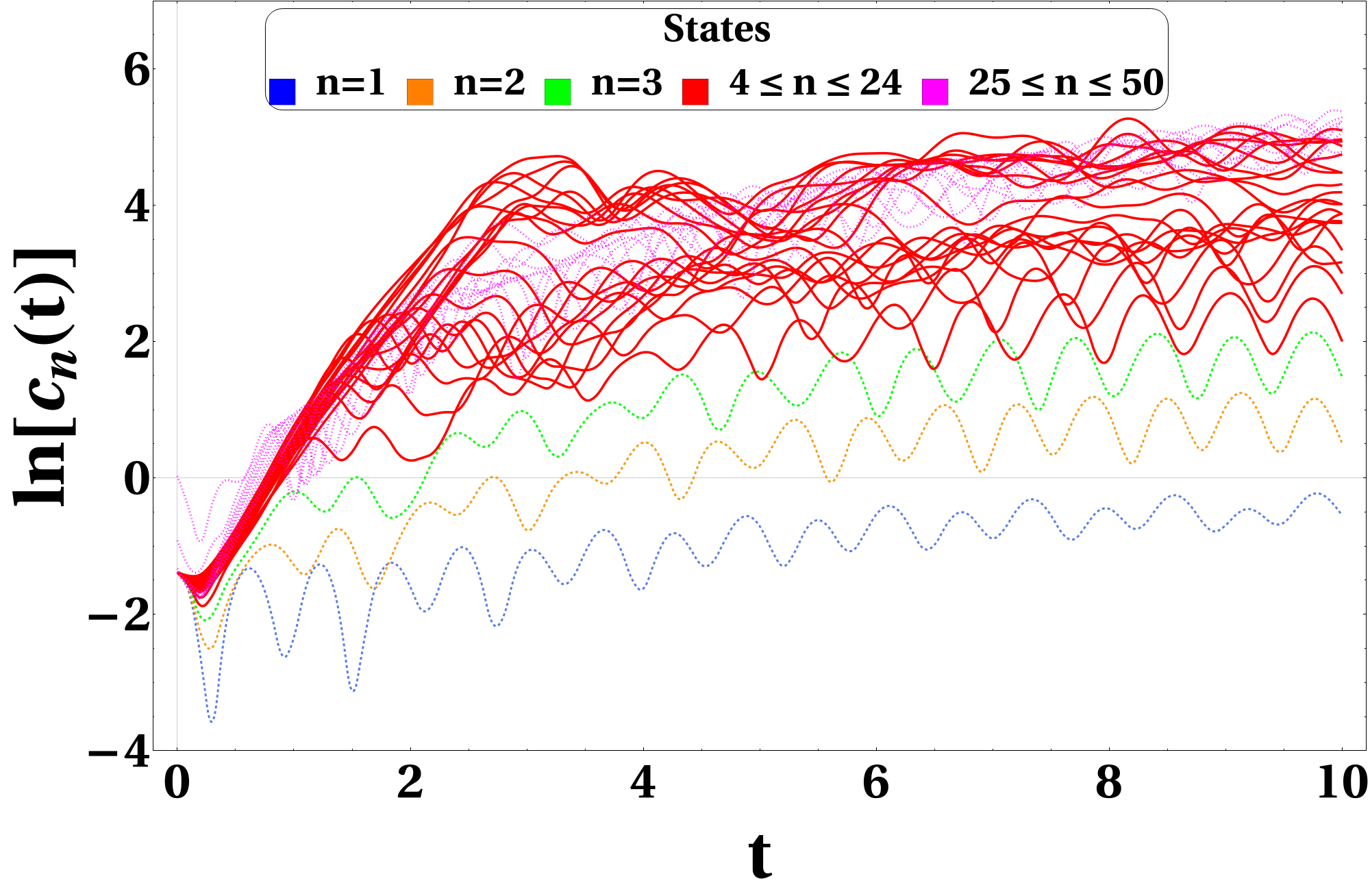
(d) $\sigma=50.0$

(e) $\sigma=0.0$

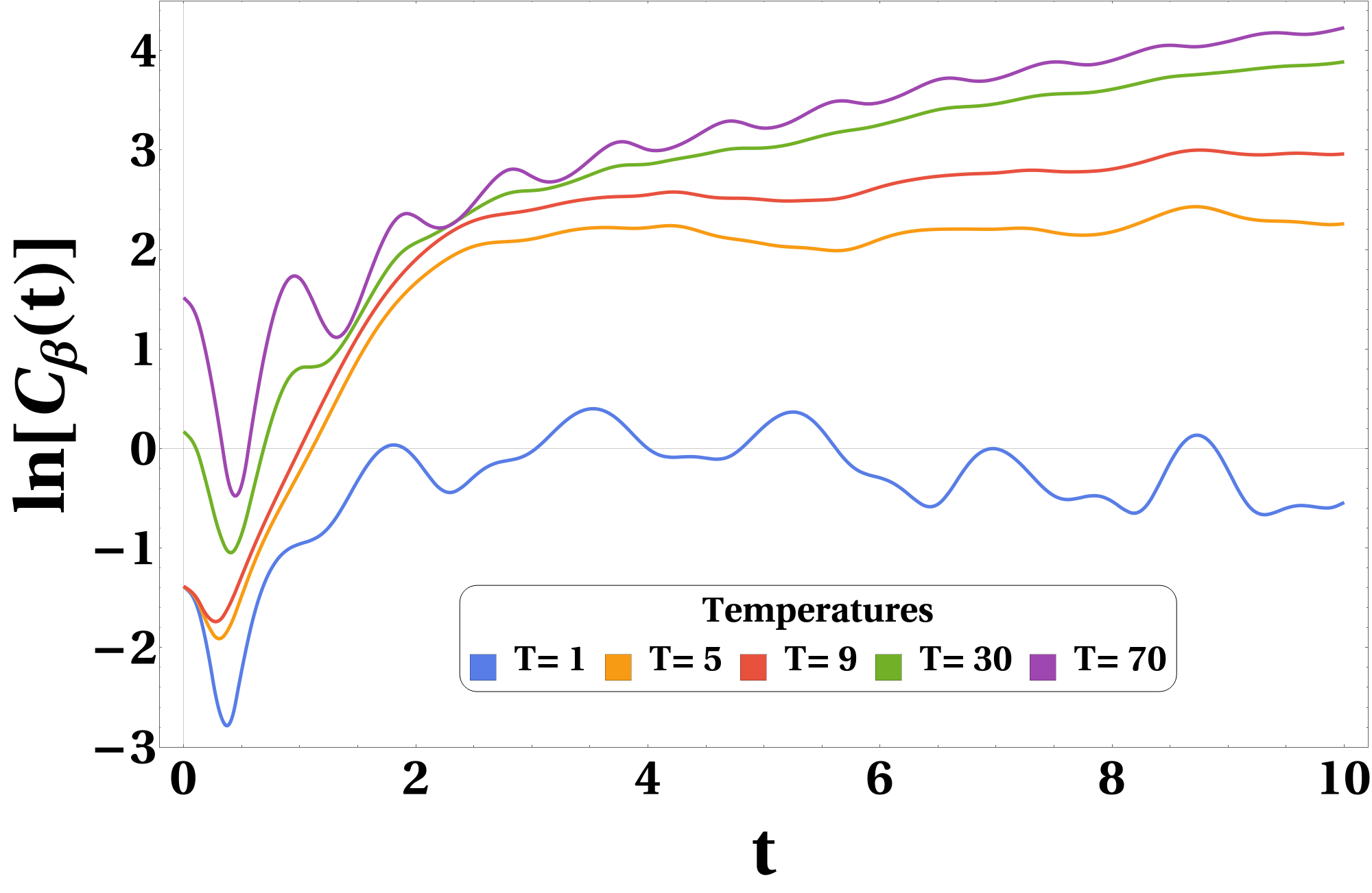
(f) $\sigma=0.15$

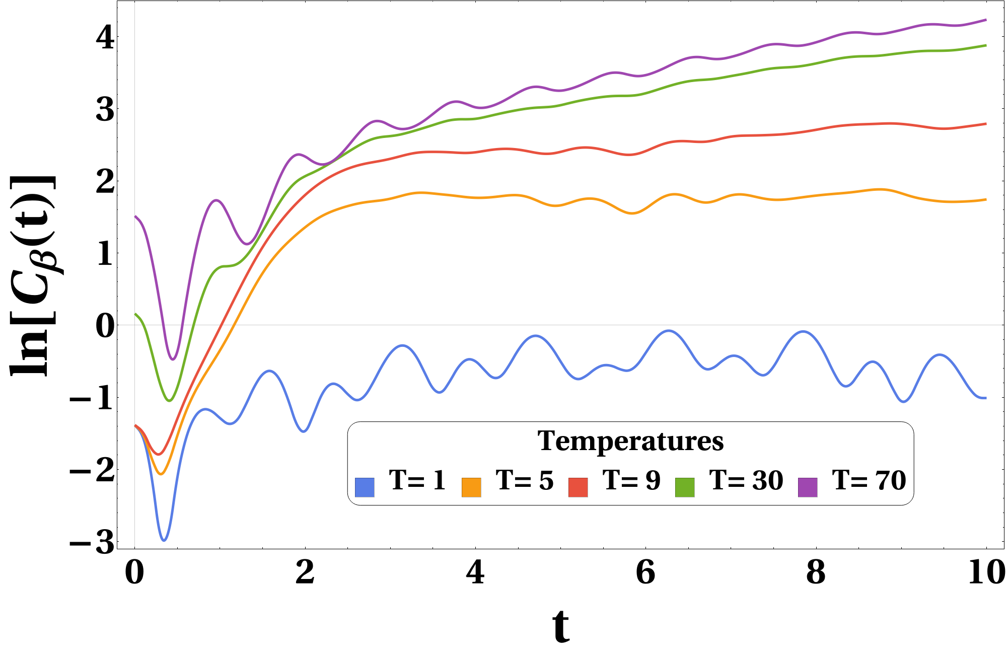
(g) $\sigma=10.0$

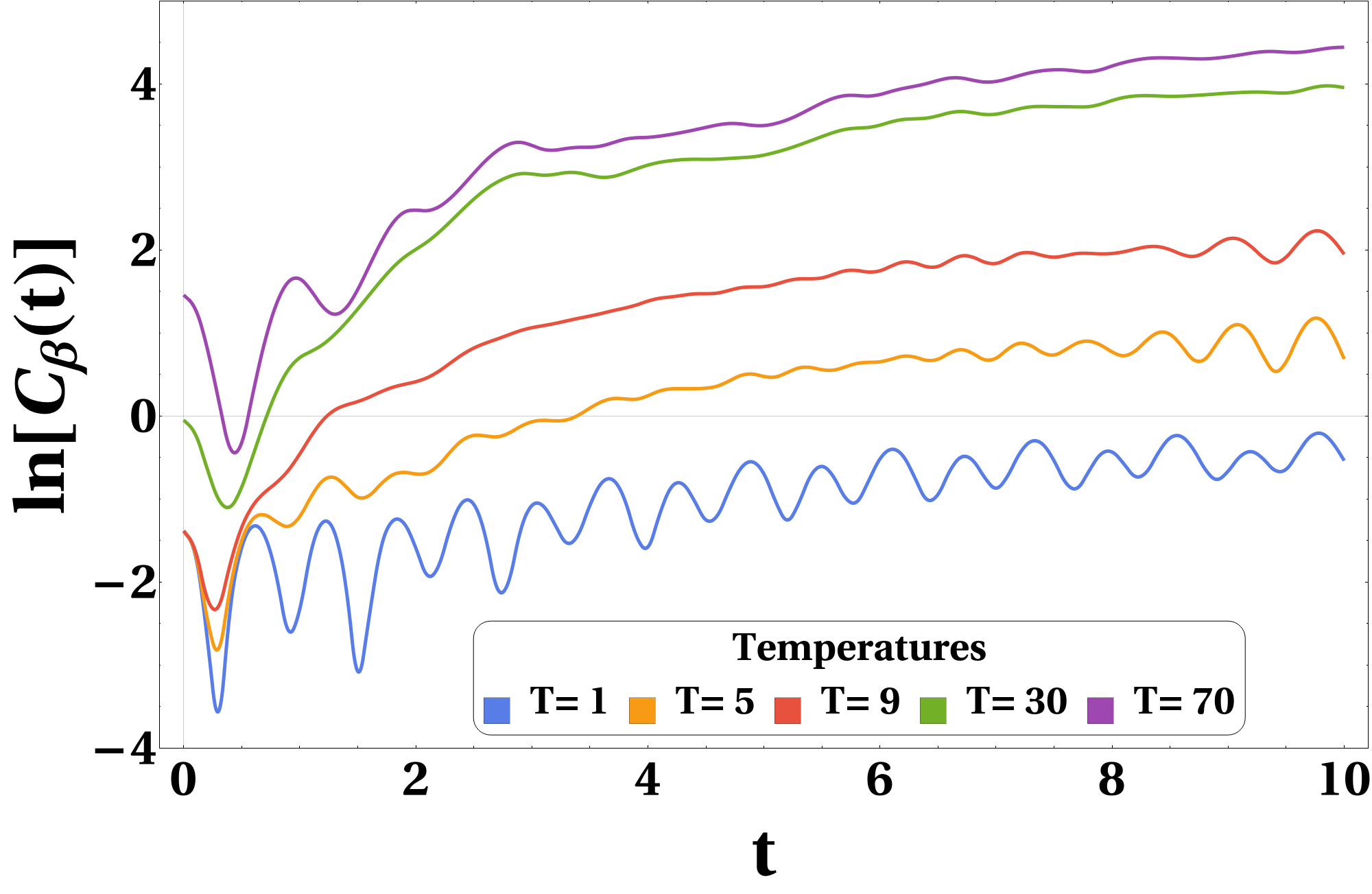
(h) $\sigma=50.0$

Figure 13: (a), (b), (c), (d) shows microcanonical OTOC and (e), (f), (g), (h) shows thermal OTOC for $Model(III)$ with different values of $\sigma$.

Considering potential for $Model(III)$(Eq.(14)), we plotted Eq.(7) and Eq.(6), for different values of $\sigma$ in Fig.(13).

Here, we find that the microcanonical OTOC shows exponential growth for energy levels near the plateau for $\sigma=0.0$ and $0.15$ in Fig.(13(a)) and in Fig.(13(b)), respectively. Similarly, the behaviour of thermal OTOC can be seen in Fig.(13(e)) and Fig.(13(f)) for the same value of $\sigma$s. However, for $\sigma=10.0$, the plateau transforms into a local maximum at $x=1.44077$ shown in Fig.(5(c)). For which the right side of this double-well potential(a local minimum) has its ground state ($5^{th}$ excited state for the whole system) close to this maximum. As a result, its growth rate falls behind the exponential regime of the $3^{rd}$ to $15^{th}$ excited states shown in the green dashed line in Fig.(13(c)). For $\sigma=50.0$, neither the plateau nor the local maximum is present, as shown in Fig.(5(d)). Nevertheless, microcanonical OTOC continues to grow exponentially at this asymmetry strength, as shown in Fig.(13(d)). Thermal OTOC also shows exponential growth at these values for higher temperatures, shown in Fig.(13(g)) and Fig.(13(h)).

V Discussion

A small symmetry-breaking term in the Hamiltonian introduces a delicate perturbation that disrupts certain classical systems’ underlying symmetries. This perturbation acts as a catalyst, initiating a cascade of non-linear resonances within the symmetry-breaking regions. This emergence of non-linear resonances often leads to the initial onset of chaos. As these regions expand, the chaotic nature of the system amplifies, resulting in an even greater degree of unpredictability and complexity.

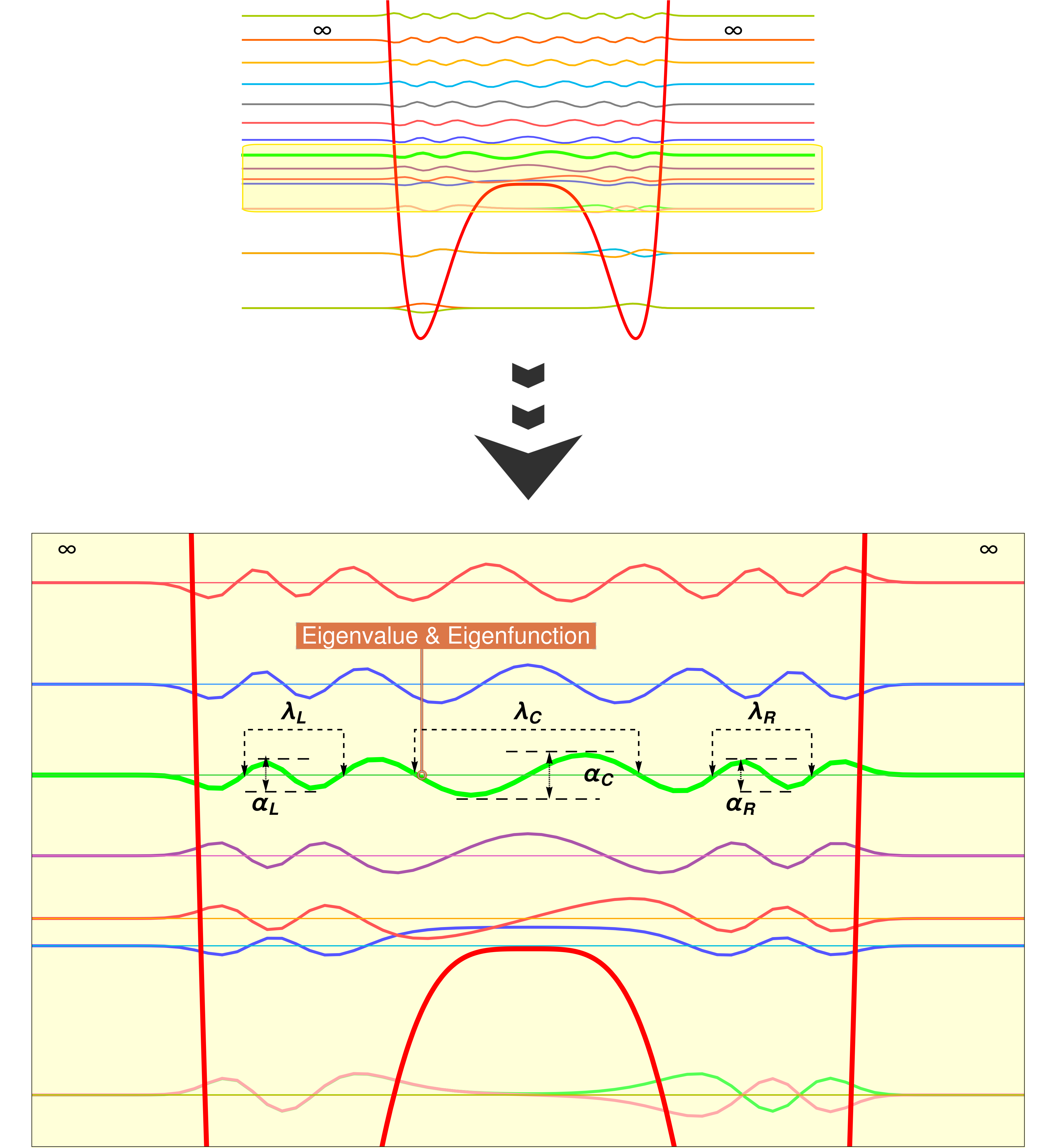
(a) $Model(III)$ with nonzero $\sigma=0.0$. The eigenstates spread near the plateau from both the directions with a slight increase in amplitude in the same direction, i.e., $\lambda_{L}<\lambda_{C}>\lambda_{R}$ and $\alpha_{L}<\alpha_{C}>\alpha_{R}$.

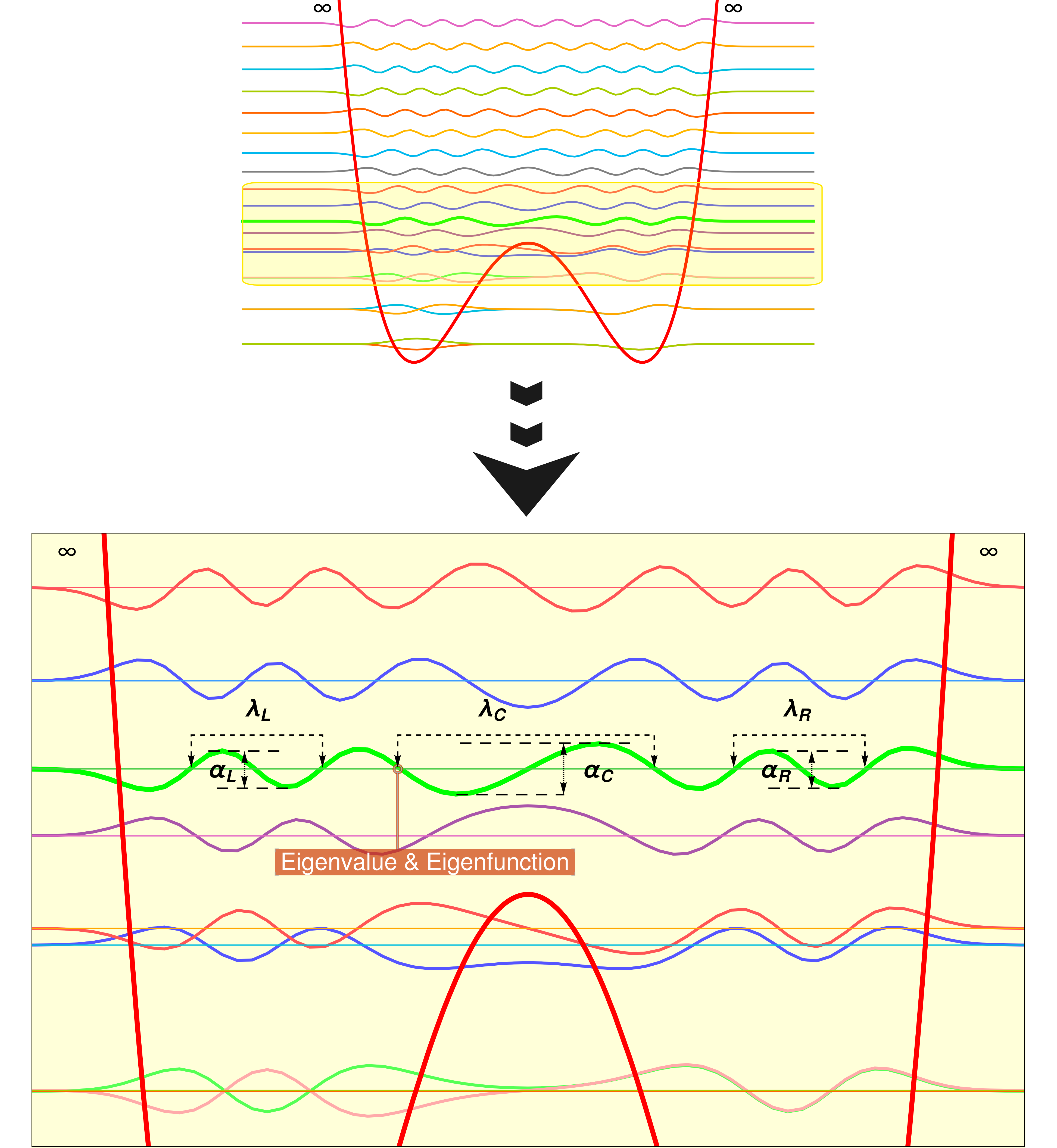
(b) $Model(I)$ with $\sigma=0$. The eigenstates spread near the hilltop from both the directions with a slight increase in amplitude in the same direction, i.e., $\lambda_{L}<\lambda_{C}>\lambda_{R}$ and $\alpha_{L}<\alpha_{C}>\alpha_{R}$.

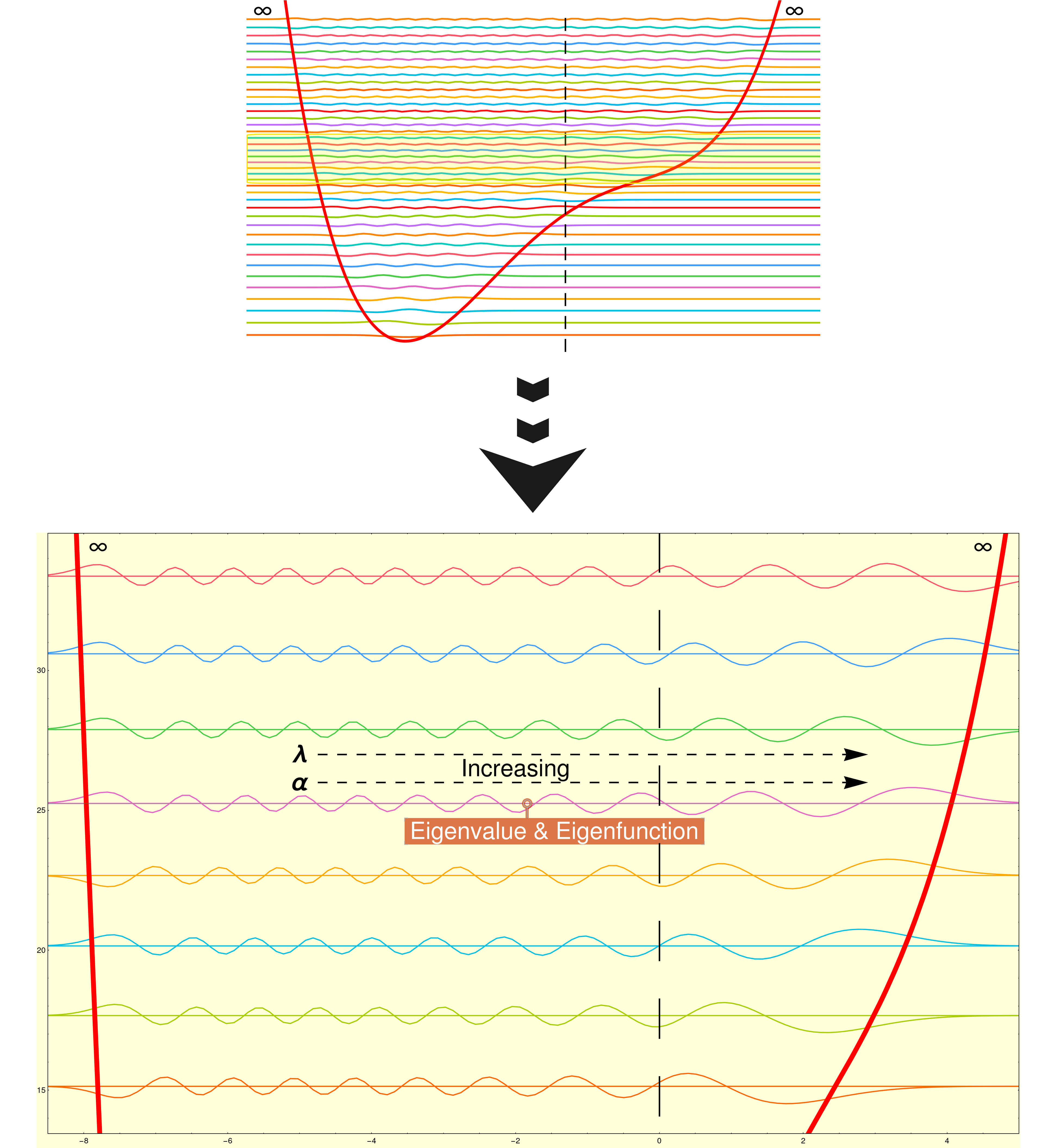
(c) $Model(I)$ with nonzero $\sigma$. In the reigion of the broken symmetry, eventhough the local maxima is absent, the eigenstates spread gradually from the left to the right with a slight increase in amplitude in the same direction.

Figure 14: Stretching of eigenstates because of symmetry breaking. $\lambda$ and $\dfrac{\alpha}{2}$ are the wavelength and amplitude of the eigenstates, respectively.

In previous studies[35, 37, 80, 38, 36, 81, 39, 82, 83], numerous authors have widely observed the exponential growth of OTOC in the vicinity of an unstable equilibrium. However, our findings indicate that introducing perturbation or a symmetry-breaking term in the potential, aimed at eliminating the unstable equilibrium from the system, does not necessarily eliminate the exponential growth of OTOC. Instead, it mitigates the growth to some extent, reducing the magnitude of the exponential behaviour yet spreading over a more significant vicinity. This happens because of the symmetry-breaking of the Hamiltonian[48, 84, 85, 86, 87, 88, 89, 90, 91, 92, 93, 94, 95, 96, 97, 98].

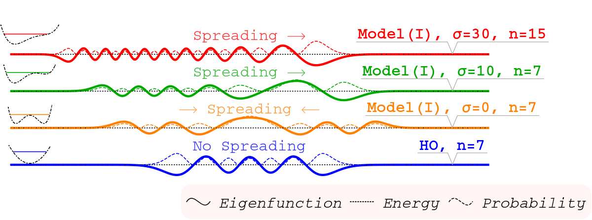
Figure 15: Stretching of eigenstates(solid line) along the width of the potential with spreading of probability distribution(dashed line) for different models.

As the symmetry breaks, asymmetry appears in potential function leading to the disappearance of degeneracy from the system. This ultimately leads to stretching and spreading of eigenfunctions, shown in Figs.(14 & 15). For $\sigma=0$, the eigenfunctions in the neighbourhood of the unstable equilibrium have longer wavelengths and higher amplitude compared to their left and right. In other words, the eigenfunctions spread around the unstable equilibrium or in broken symmetry region shown in Figs.(14(a) & 14(b)). This spreading behaviour continues as we keep increasing the value of $\sigma$. For specific values of $\sigma$, when we eliminate the unstable equilibrium, this spreading behaviour continues to exist, but instead of spreading in the middle, it now spreads from left to right as shown in Fig.(14(c)). This symmetry-breaking effect can be seen for all three models mentioned above.

The irregularities in the eigenfunctions, stemming from the symmetry breaking, are captured by the exponential growth of the four-point OTOC. In other words, the exponential growth primarily originates from the symmetry-breaking in the potential rather than the presence of a local maximum. We have also observed that as the strength of the perturbation increases, the broken symmetric regions widen. Consequently, a broader range of consecutive eigenstates exhibits exponential growth, albeit for shorter durations. As we move towards higher regions in the potential wells, the energy values become sufficiently large and suppress the impact of symmetry breaking on the eigenfunctions. Consequently, the stretching and localisation gradually diminish, decreasing the results obtained from the four-point OTOC.

However, if we continue to increase the strength of the perturbation, the last term in the potential becomes dominant and drives the system. At this point, the system loses its original nature and transforms into a new system altogether, where the previously observed behaviour of the OTOC no longer manifests.

Loschmidt Echo

Loschmidt echo measures the revival occurring under an imperfect time-reversal procedure applied to a complex quantum system. This tool quantifies the sensitivity of quantum evolution to isospectral perturbations. Any spectral quantity will remain unaffected, but the Loschmidt echo will generally decay[99, 100, 101, 102, 103, 104, 105, 106].

Different decay behaviours in quantum fidelity are well-defined based on factors like perturbation strength, system complexity, dimension, and initial state. Reviews by Gorin et al.[101] and Jacquod et al. [20] discuss fidelity properties, decoherence, and irreversibility. Notable decay regimes include Lyapunov[17], Fermi-Golden-Rule[17, 107], and perturbative[107, 108, 109], observed in both regular and chaotic systems[110, 111, 112]. This contrasts the typical view of exponential decay as chaotic; to our knowledge, no theoretical model is currently able to quantitatively explain the exponential decay of the Loschmidt echo in integrable systems.

Mathematically, the Loschmidt echo is then defined as,

$$M(t)=\quantity|A(t)|^{2}=\quantity|\expectationvalue{e^{i\hat{\mathcal{H}}_{2}t/\hbar}e^{-i\hat{\mathcal{H}}_{1}t/\hbar}}{\Psi_{0}}|^{2}$$ (13)

where $A(t)$ is the Loschmidt amplitude. It quantifies the “distance” (in the Hilbert space) between the state $e^{-i\hat{\mathcal{H}_{1}}t}\ket{\psi_{0}}$, resulting from the initial state $\ket{\psi_{0}}$ in the course of evolution through a time $t$ under the Hamiltonian $\mathcal{H}_{1}$, and the state $e^{-i\hat{\mathcal{H}_{2}}t}\ket{\psi_{0}}$ obtained by evolving the same initial state through the same time $t$, but under a slightly different perturbed Hamiltonian $\mathcal{H}_{2}$. The LE, by construction, equals unity for t = 0 and typically decays further in time.

Table 1: Values of perturbation strength($\Lambda$) for different values of asymmetry parameter($\sigma$).

$\bm{\sigma}$	$\bm{\Lambda}$
	$Model(I)$	$Model(II)$	$Model(III)$
0.0	0.0	0.0	0.0
0.15	0.0188	0.0959	0.0229819
10.0	1.2500	6.3900	1.53214
30.0	3.7500	19.1703	-
50.0	-	-	7.66066
70.0	8.7500	-	-

Perfect recovery of $\ket{\psi_{0}}$ would be achieved by choosing $\mathcal{H}_{2}=\mathcal{H}_{1}$, which leads to $M(t)=1$, but this is an impossible task in realistic problems and $M(t)$ is usually a decreasing function in $t$. The notion of time reversal i.e. a backward time evolution from $t$ to $0$ under $\mathcal{H}_{2}$ is equivalent to the forward evolution between $t$ and $2t$ under the Hamiltonian $-\mathcal{H}_{2}$.

Now, to compute Eq.(13), we follow the algorithm given by A. Peres in [16]. It follows that

$$\begin{split}M(t)&=\quantity|\expectationvalue{e^{i(\hat{\mathcal{H}}_{2}-\hat{\mathcal{H}}_{1})t/\hbar}}{\Psi_{0}}|^{2}\\ &=\quantity|\expectationvalue{e^{i\Lambda\hat{x}t/\hbar}}{\Psi_{0}}|^{2}\\ &=\quantity|\expectationvalue{e^{i\hat{x}\tau}}{\Psi_{0}}|^{2}\end{split}$$ (14)

where $\tau=\dfrac{\Lambda t}{\hbar}$ and we assume that $\Lambda\hat{x}(=\hat{\mathcal{H}}_{2}-\hat{\mathcal{H}}_{1})$ is classically small but quantum mechanically significant such that the perturbation does not change the topology of the trajectories but introduces a phase difference.

For regular systems, $M(t)$ must oscillates with a fairly large amplitude. Strictly speaking, $M(t)$ is almost periodic. On the other hand, if $\mathcal{H}_{1}$ is chaotic, $M(t)$ is small. Another fact is that the initial decay rate of $M(t)$ for regular systems is fairly same as for chaotic systems. It is in fact completely independent of Hamiltonian.

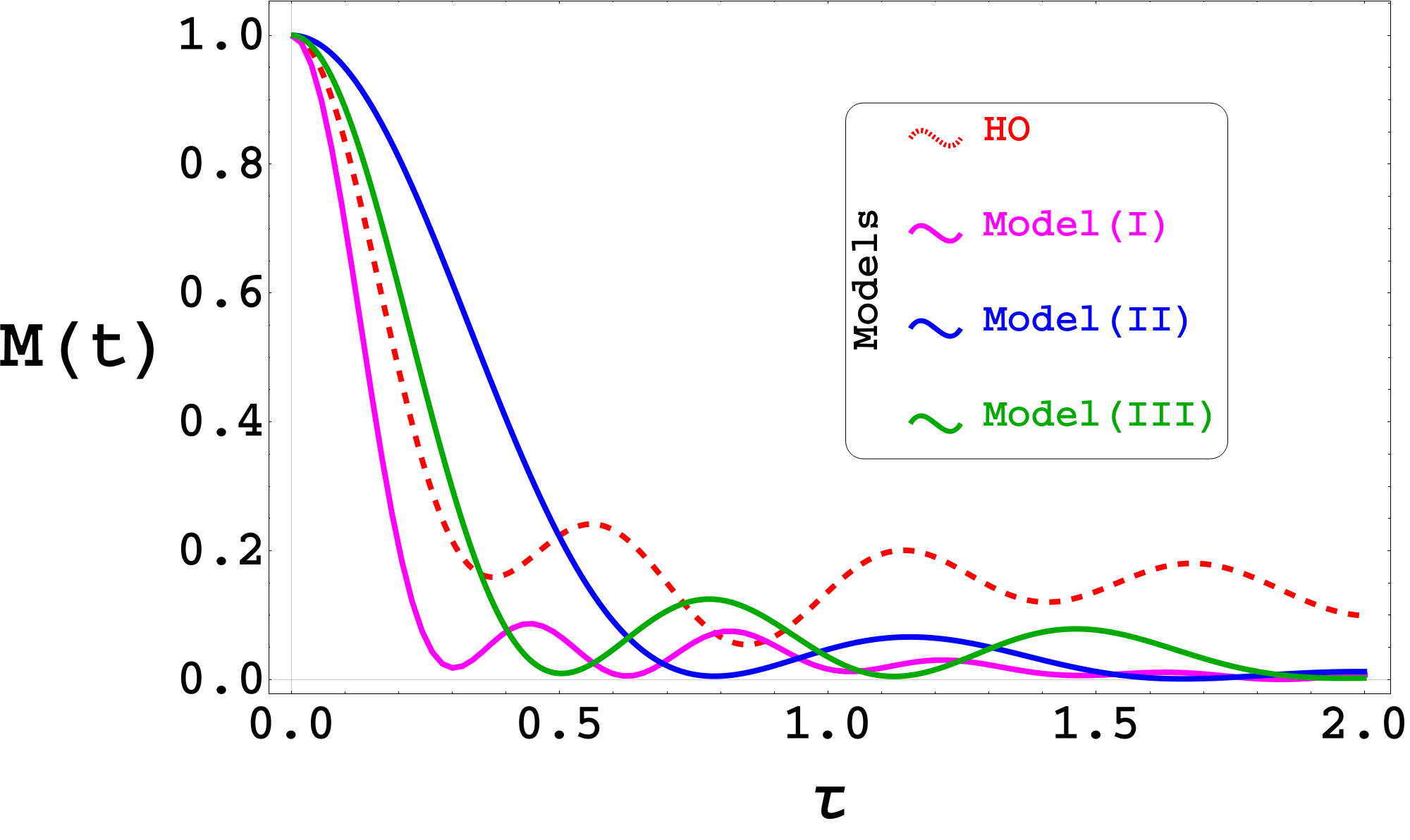
Figure 16: Loschmidt Echo of Harmonic Oscillator(HO), $Model(I)$, $Model(II)$, and $Model(III)$.

For varying $\Lambda$ values as outlined in Table(1), our numerical investigation reveals an initial exponential decay followed by anticipated low-amplitude oscillations in the LE. Fig. (16) illustrates the compilation of LEs encompassing the Harmonic Oscillator(HO), as well as $Models(I)$, $(II)$, and $(III)$. In particular, after the initial decay, the LE displays significant amplitude fluctuations in the HO case. However, intriguingly, our investigated models demonstrate comparatively smaller fluctuations in their LE behaviour. This contrast in fluctuation amplitude between the HO and our models suggests the presence of distinctive dynamical behaviours, potentially indicating unconventional characteristics in our systems.

Spectral Form Factor

Another quantity related to OTOC and Loschmidt Echo is the spectral form factor(SFF) [113, 114, 115, 25, 9]. In a chaotic system, the SFF exhibits a dip-ramp-plateau structure, while the ramp is not present in integrable systems. To alleviate the computation and to achieve more physical intuition, with the analytical continuance, the partition function can be defined as

$$\mathcal{Z}(\beta,t)=Z(\beta+it)=\Tr(e^{-\beta\mathcal{H}-i\mathcal{H}t})$$ (15)

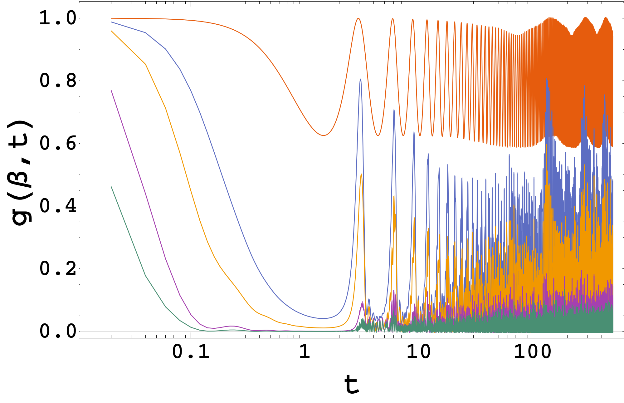
(a) $Model(I)$ with $\sigma=30$

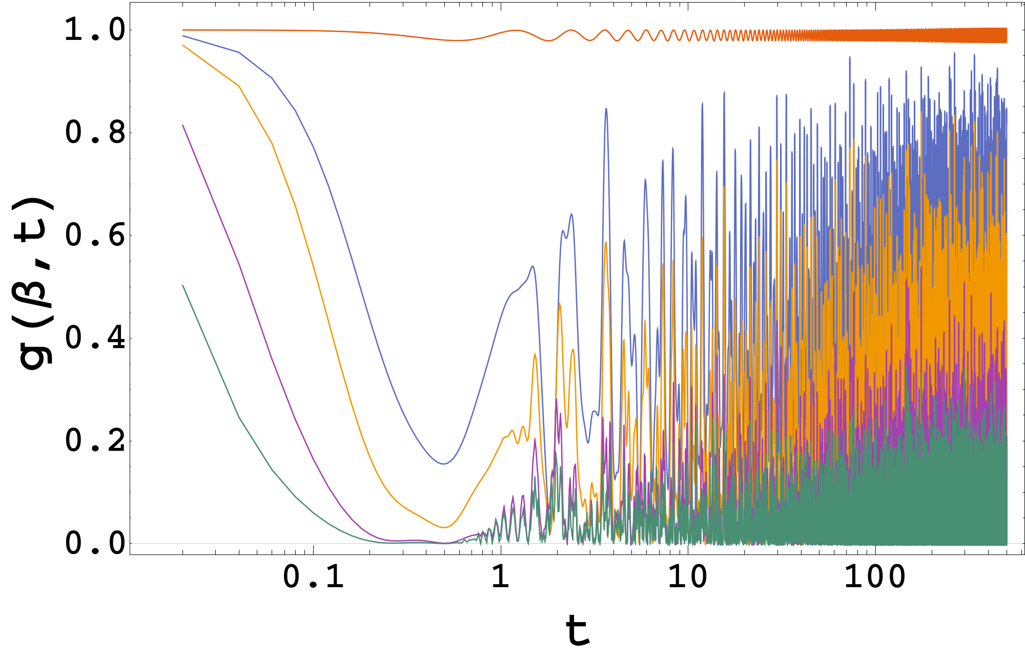
(b) $Model(II)$ with $\sigma=10$

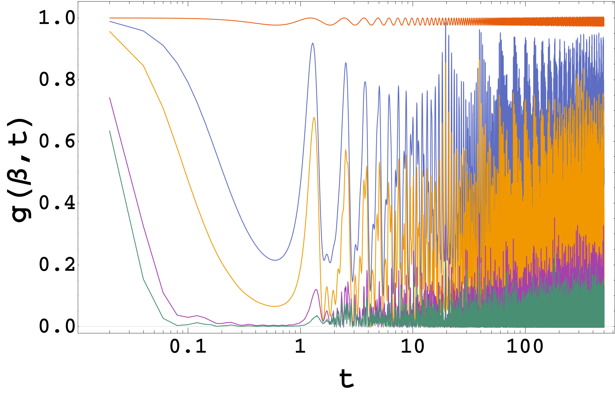
(c) $Model(III)$ with $\sigma=50$

Figure 17: SFF as a function of time for five different temperatures $T=$ ($\blacksquare$$\rightarrow 1$), ($\blacksquare$$\rightarrow 5$), ($\blacksquare$$\rightarrow 9$), ($\blacksquare$$\rightarrow 30$) and ($\blacksquare$$\rightarrow 70$).

where $\mathcal{Z}$ is the partition function.The time average of $\mathcal{Z}(\beta,t)$ vanishes, so it is an oscillating function around zero. At late times $\mathcal{Z}(\beta,t)$ also oscillates erratically.

Normalizing it by the partition function, we can determine the size of fluctuations:

$$g(\beta,t)=\absolutevalue{\frac{\mathcal{Z}(\beta,t)}{Z(\beta)}}^{2}=\frac{1}{\absolutevalue{Z(\beta)}^{2}}\sum_{m,n}e^{-\beta(E_{m}+E_{n})}e^{i(E_{m}-E_{n})t}$$ (16)

The function $g(\beta,t)$ is the desired SFF.

The SFF of a chaotic system shows a distinct dip-ramp-plateau pattern[7, 116, 117, 25, 118, 9, 119, 120]. The initial decay represents a short-time slope following a ramp due to long-range energy level repulsion. The dip marks the shift from the slope to the ramp. Finally, the plateau arises from finite Hilbert space dimensions approaching a constant value, $\mathcal{Z}(2\beta)/\mathcal{Z}(\beta)^{2}$, when no degeneracies exist.

The SFFs for all three models are depicted in Fig.(17). At low temperatures, $g(\beta,t)$ initially decreases and returns to its initial value. In contrast, $g(\beta,t)$ exhibits an initial drop at high temperatures, followed by a rise and eventually settles into a fluctuating plateau at late times. The high-temperature behaviour of $g(\beta,t)$ bears some resemblance to that of a single random matrix.

VI Conclusion

The exponential growth of both microcanonical and thermal OTOC in the neighbourhood of the local maximum of an IHO potential is a well-known fact; however, it is incomplete. With several examples, we demonstrate that even without a local maximum, OTOC shows exponential growth in the same neighbourhood, and in some cases, this region broadens. Hence, the cause of this growth, in general, cannot be due to the presence of a local maximum but due to the symmetry breaking in the Hamiltonian. The behaviour of OTOC in a single-well potential is periodic. However, by varying an order parameter, when we break the existing symmetry in the Hamiltonian of this system, it ends up with one local maximum and two minima ($Model(I)$) or two maxima and three minima ($Model(III)$) or a plateau and two minima ($Model(III)$). Irrespective of their shapes, early time exponential growth of OTOC comes into the picture in the neighbourhood of the broken symmetric regions, which happens to be around the local maxima of these wells. When we further break the symmetries and make the systems free of any local maximum, OTOC continues to show exponential growth in a broader region where symmetry breakings occur. Chaos first appears in the neighbourhood of the broken symmetric regions, and as the parameter responsible for it strengthens, the chaotic regions also expand. Here, OTOC, a quantum mechanical diagnostic tool for chaos, beautifully captures the effects of symmetry-breaking, although the models under study are regular integrable systems. Therefore, our study provides compelling evidence supporting the importance of symmetry breaking when analysing the behaviour of complex quantum mechanical systems, which has important implications for understanding various physical systems, from condensed matter systems to black holes.

Overall, the study of OTOCs and symmetry breaking has important implications for our understanding of quantum chaos and the behaviour of complex systems. We aim to extend our research further into the matter considering coupled systems and particles with spin.

References

- [1] A. Wolf, J. B. Swift, H. L. Swinney, and J. A. Vastano, “Determining lyapunov exponents from a time series,” Physica D: Nonlinear Phenomena, vol. 16, no. 3, pp. 285–317, 1985.
- [2] M.-F. Danca and N. Kuznetsov, “Matlab code for lyapunov exponents of fractional-order systems,” International Journal of Bifurcation and Chaos, vol. 28, no. 05, p. 1850067, 2018.
- [3] F. Christiansen and H. H. Rugh, “Computing lyapunov spectra with continuous gram - schmidt orthonormalization,” Nonlinearity, vol. 10, p. 1063, sep 1997.
- [4] S. Habib and R. D. Ryne, “Symplectic calculation of lyapunov exponents,” Phys. Rev. Lett., vol. 74, pp. 70–73, Jan 1995.
- [5] O. Bohigas, M. J. Giannoni, and C. Schmit, “Characterization of chaotic quantum spectra and universality of level fluctuation laws,” Phys. Rev. Lett., vol. 52, pp. 1–4, Jan 1984.
- [6] F. Haake, S. Gnutzmann, and M. Kuś, Quantum Signatures of Chaos. Springer Series in Synergetics, Springer International Publishing, 2019.
- [7] J. S. Cotler, G. Gur-Ari, M. Hanada, J. Polchinski, P. Saad, S. H. Shenker, A. Stanford, Douglasand Streicher, and M. Tezuka, “Black holes and random matrices,” Journal of High Energy Physics, vol. 2017, p. 118, May 2017.
- [8] A. Gaikwad and R. Sinha, “Spectral form factor in non-gaussian random matrix theories,” Phys. Rev. D, vol. 100, p. 026017, Jul 2019.
- [9] J. Liu, “Spectral form factors and late time quantum chaos,” Phys. Rev. D, vol. 98, p. 086026, Oct 2018.
- [10] T. Guhr, A. Müller–Groeling, and H. A. Weidenmüller, “Random-matrix theories in quantum physics: common concepts,” Physics Reports, vol. 299, no. 4, pp. 189–425, 1998.
- [11] X. Wang, S. Ghose, B. C. Sanders, and B. Hu, “Entanglement as a signature of quantum chaos,” Phys. Rev. E, vol. 70, p. 016217, Jul 2004.
- [12] P. Zanardi, C. Zalka, and L. Faoro, “Entangling power of quantum evolutions,” Phys. Rev. A, vol. 62, p. 030301, Aug 2000.
- [13] A. Lakshminarayan, “Entangling power of quantized chaotic systems,” Phys. Rev. E, vol. 64, p. 036207, Aug 2001.
- [14] P. Zanardi, “Entanglement of quantum evolutions,” Phys. Rev. A, vol. 63, p. 040304, Mar 2001.
- [15] N. Anand, G. Styliaris, M. Kumari, and P. Zanardi, “Quantum coherence as a signature of chaos,” Phys. Rev. Research, vol. 3, p. 023214, Jun 2021.
- [16] A. Peres, “Stability of quantum motion in chaotic and regular systems,” Phys. Rev. A, vol. 30, pp. 1610–1615, Oct 1984.
- [17] R. A. Jalabert and H. M. Pastawski, “Environment-independent decoherence rate in classically chaotic systems,” Phys. Rev. Lett., vol. 86, pp. 2490–2493, Mar 2001.
- [18] P. Jacquod, “Semiclassical time evolution of the reduced density matrix and dynamically assisted generation of entanglement for bipartite quantum systems,” Phys. Rev. Lett., vol. 92, p. 150403, Apr 2004.
- [19] C. Petitjean and P. Jacquod, “Lyapunov generation of entanglement and the correspondence principle,” Phys. Rev. Lett., vol. 97, p. 194103, Nov 2006.
- [20] P. Jacquod and C. Petitjean, “Decoherence, entanglement and irreversibility in quantum dynamical systems with few degrees of freedom,” Advances in Physics, vol. 58, no. 2, pp. 67–196, 2009.
- [21] A. I. Larkin and Y. N. Ovchinnikov, “Quasiclassical Method in the Theory of Superconductivity,” Soviet Journal of Experimental and Theoretical Physics, vol. 28, p. 1200, june 1969.
- [22] I. García-Mata, M. Saraceno, R. A. Jalabert, A. J. Roncaglia, and D. A. Wisniacki, “Chaos signatures in the short and long time behavior of the out-of-time ordered correlator,” Phys. Rev. Lett., vol. 121, p. 210601, Nov 2018.
- [23] R. N. Das, S. Dutta, and A. Maji, “Generalised out-of-time-order correlator in supersymmetric quantum mechanics,” 2022.
- [24] P. Zanardi and N. Anand, “Information scrambling and chaos in open quantum systems,” Phys. Rev. A, vol. 103, p. 062214, Jun 2021.
- [25] P. Romatschke, “Quantum mechanical out-of-time-ordered-correlators for the anharmonic (quartic) oscillator,” Journal of High Energy Physics, vol. 2021, p. 30, Jan 2021.
- [26] M. A. Prado Reynoso, G. J. Delben, M. Schlesinger, and M. W. Beims, “Finite-time lyapunov fluctuations and the upper bound of classical and quantum out-of-time-ordered expansion rate exponents,” Phys. Rev. E, vol. 106, p. L062201, Dec 2022.
- [27] R. J. Lewis-Swan, A. Safavi-Naini, J. J. Bollinger, and A. M. Rey, “Unifying scrambling, thermalization and entanglement through measurement of fidelity out-of-time-order correlators in the dicke model,” Nature Communications, vol. 10, p. 1581, Apr 2019.
- [28] R. J. Garcia, Y. Zhou, and A. Jaffe, “Quantum scrambling with classical shadows,” Phys. Rev. Res., vol. 3, p. 033155, Aug 2021.
- [29] A. Lakshminarayan, “Out-of-time-ordered correlator in the quantum bakers map and truncated unitary matrices,” Phys. Rev. E, vol. 99, p. 012201, Jan 2019.
- [30] E. B. Rozenbaum, S. Ganeshan, and V. Galitski, “Lyapunov exponent and out-of-time-ordered correlator’s growth rate in a chaotic system,” Phys. Rev. Lett., vol. 118, p. 086801, Feb 2017.
- [31] F. Meier, M. Steinhuber, J. D. Urbina, D. Waltner, and T. Guhr, “Signatures of the interplay between chaos and local criticality on the dynamics of scrambling in many-body systems,” Phys. Rev. E, vol. 107, p. 054202, May 2023.
- [32] T. Ali, A. Bhattacharyya, S. S. Haque, E. H. Kim, N. Moynihan, and J. Murugan, “Chaos and complexity in quantum mechanics,” Phys. Rev. D, vol. 101, p. 026021, Jan 2020.
- [33] I. Kukuljan, S. c. v. Grozdanov, and T. c. v. Prosen, “Weak quantum chaos,” Phys. Rev. B, vol. 96, p. 060301, Aug 2017.
- [34] E. M. Fortes, I. García-Mata, R. A. Jalabert, and D. A. Wisniacki, “Gauging classical and quantum integrability through out-of-time-ordered correlators,” Phys. Rev. E, vol. 100, p. 042201, Oct 2019.
- [35] K. Hashimoto, K.-B. Huh, K.-Y. Kim, and R. Watanabe, “Exponential growth of out-of-time-order correlator without chaos: inverted harmonic oscillator,” Journal of High Energy Physics, vol. 2020, p. 68, Nov 2020.
- [36] R. A. Kidd, A. Safavi-Naini, and J. F. Corney, “Saddle-point scrambling without thermalization,” Phys. Rev. A, vol. 103, p. 033304, Mar 2021.
- [37] W. Kirkby, D. H. J. O’Dell, and J. Mumford, “False signals of chaos from quantum probes,” Phys. Rev. A, vol. 104, p. 043308, Oct 2021.
- [38] T. Xu, T. Scaffidi, and X. Cao, “Does scrambling equal chaos?,” Phys. Rev. Lett., vol. 124, p. 140602, Apr 2020.
- [39] T. Morita, “Extracting classical lyapunov exponent from one-dimensional quantum mechanics,” Phys. Rev. D, vol. 106, p. 106001, Nov 2022.
- [40] K. Hashimoto, K. Murata, and R. Yoshii, “Out-of-time-order correlators in quantum mechanics,” Journal of High Energy Physics, vol. 2017, p. 138, Oct 2017.
- [41] P. Garbaczewski, V. A. Stephanovich, and G. Engel, “Electron spectra in double quantum wells of different shapes,” New Journal of Physics, vol. 24, p. 033052, mar 2022.
- [42] N. Aquino, J. Garza, G. Campoy, and A. Vela, “Energy eigenvalues for free and confined triple-well potentials,” Revista Mexicana De Fisica, vol. 57, pp. 46–52, 2011.
- [43] K. Wittmann W., E. R. Castro, A. Foerster, and L. F. Santos, “Interacting bosons in a triple well: Preface of many-body quantum chaos,” Phys. Rev. E, vol. 105, p. 034204, Mar 2022.
- [44] R. J. Damburg, R. K. Propin, and Y. I. Ryabykh, “Perturbation theory for the triple-well anharmonic oscillator,” Phys. Rev. A, vol. 41, pp. 1218–1224, Feb 1990.
- [45] L. N. Hand and J. D. Finch, “Chaotic dynamics,” in Analytical Mechanics, p. 423–492, Cambridge University Press, 1998.
- [46] L. Reichl, “Bounded quantum systems,” in The Transition to Chaos: Conservative Classical and Quantum Systems, pp. 195–237, Cham: Springer International Publishing, 2021.
- [47] P. Bracken, “Introductory chapter: Dynamical symmetries and quantum chaos,” in Research Advances in Chaos Theory (P. Bracken, ed.), ch. 1, Rijeka: IntechOpen, 2020.
- [48] W.-M. Zhang, D. H. Feng, J.-M. Yuan, and S.-J. Wang, “Integrability and nonintegrability of quantum systems: Quantum integrability and dynamical symmetry,” Phys. Rev. A, vol. 40, pp. 438–447, Jul 1989.
- [49] G.-H. Sun, Q. Dong, V. B. Bezerra, and S.-H. Dong, “Exact solutions of an asymmetric double well potential,” Journal of Mathematical Chemistry, vol. 60, pp. 605–612, Apr 2022.
- [50] G. Theocharis, P. G. Kevrekidis, D. J. Frantzeskakis, and P. Schmelcher, “Symmetry breaking in symmetric and asymmetric double-well potentials,” Phys. Rev. E, vol. 74, p. 056608, Nov 2006.
- [51] Y. Nambu, “Dynamical symmetry breaking,” in Broken Symmetry, pp. 436–451, 1995.
- [52] S. Sarkar and J. S. Satchell, “Quantum chaos in the lorenz equations with symmetry breaking,” Phys. Rev. A, vol. 35, pp. 398–405, Jan 1987.
- [53] R. A. Jalabert, I. García-Mata, and D. A. Wisniacki, “Semiclassical theory of out-of-time-order correlators for low-dimensional classically chaotic systems,” Phys. Rev. E, vol. 98, p. 062218, Dec 2018.
- [54] J. S. Cotler, D. Ding, and G. R. Penington, “Out-of-time-order operators and the butterfly effect,” Annals of Physics, vol. 396, pp. 318–333, 2018.
- [55] S. S. Haque and B. Underwood, “Squeezed out-of-time-order correlator and cosmology,” Phys. Rev. D, vol. 103, p. 023533, Jan 2021.
- [56] K. Y. Bhagat, B. Bose, S. Choudhury, S. Chowdhury, R. N. Das, S. G. Dastider, N. Gupta, A. Maji, G. D. Pasquino, and S. Paul, “The generalized otoc from supersymmetric quantum mechanics—study of random fluctuations from eigenstate representation of correlation functions,” Symmetry, vol. 13, no. 1, 2021.
- [57] I. García-Mata, R. A. Jalabert, and D. A. Wisniacki, “Out-of-time-order correlations and quantum chaos,” Scholarpedia, vol. 18, no. 4, p. 55237, 2023. revision #199677.
- [58] J. Chávez-Carlos, B. López-del Carpio, M. A. Bastarrachea-Magnani, P. Stránský, S. Lerma-Hernández, L. F. Santos, and J. G. Hirsch, “Quantum and classical lyapunov exponents in atom-field interaction systems,” Phys. Rev. Lett., vol. 122, p. 024101, Jan 2019.
- [59] E. B. Rozenbaum, S. Ganeshan, and V. Galitski, “Universal level statistics of the out-of-time-ordered operator,” Phys. Rev. B, vol. 100, p. 035112, Jul 2019.
- [60] R. K. Shukla, A. Lakshminarayan, and S. K. Mishra, “Out-of-time-order correlators of nonlocal block-spin and random observables in integrable and nonintegrable spin chains,” Phys. Rev. B, vol. 105, p. 224307, Jun 2022.
- [61] M. Steinhuber, P. Schlagheck, J.-D. Urbina, and K. Richter, “A dynamical transition from localized to uniform scrambling in locally hyperbolic systems,” 2023.
- [62] J. Maldacena, S. H. Shenker, and D. Stanford, “A bound on chaos,” Journal of High Energy Physics, vol. 2016, p. 106, Aug 2016.
- [63] M. Zonnios, J. Levinsen, M. M. Parish, F. A. Pollock, and K. Modi, “Signatures of quantum chaos in an out-of-time-order tensor,” Phys. Rev. Lett., vol. 128, p. 150601, Apr 2022.
- [64] T. Akutagawa, K. Hashimoto, T. Sasaki, and R. Watanabe, “Out-of-time-order correlator in coupled harmonic oscillators,” Journal of High Energy Physics, vol. 2020, Aug 2020.
- [65] A. Bhattacharyya, W. Chemissany, S. S. Haque, J. Murugan, and B. Yan, “The multi-faceted inverted harmonic oscillator: Chaos and complexity,” SciPost Phys. Core, vol. 4, p. 002, 2021.
- [66] S. Gentilini, M. C. Braidotti, G. Marcucci, E. DelRe, and C. Conti, “Physical realization of the glauber quantum oscillator,” Scientific Reports, vol. 5, p. 15816, Nov 2015.
- [67] V. Subramanyan, S. S. Hegde, S. Vishveshwara, and B. Bradlyn, “Physics of the inverted harmonic oscillator: From the lowest landau level to event horizons,” Annals of Physics, vol. 435, p. 168470, 2021. Special issue on Philip W. Anderson.
- [68] S. Choudhury, S. P. Selvam, and K. Shirish, “Circuit complexity from supersymmetric quantum field theory with morse function,” Symmetry, vol. 14, p. 1656, aug 2022.
- [69] Z.-M. Xu, B. Wu, and W.-L. Yang, “van der waals fluid and charged ads black hole in the landau theory,” Classical and Quantum Gravity, vol. 38, p. 205008, sep 2021.
- [70] R. Li and J. Wang, “Generalized free energy landscape of a black hole phase transition,” Phys. Rev. D, vol. 106, p. 106015, Nov 2022.
- [71] S.-W. Wei, Y.-X. Liu, and Y.-Q. Wang, “Dynamic properties of thermodynamic phase transition for five-dimensional neutral gauss-bonnet ads black hole on free energy landscape,” Nuclear Physics B, vol. 976, p. 115692, 2022.
- [72] Y.-Z. Du, H.-F. Li, F. Liu, and L.-C. Zhang, “Dynamic property of phase transition for non-linear charged anti-de sitter black holes *,” Chinese Physics C, vol. 46, p. 055104, may 2022.
- [73] V. I. Kuvshinov, A. V. Kuzmin, and V. A. Piatrou, “Asymmetric double well system as effective model for the kicked one,” 2011.
- [74] R. P. McRae and B. C. Garrett, “Anharmonic corrections to variational transition state theory calculations of rate constants for a model activated reaction in solution,” The Journal of Chemical Physics, vol. 98, pp. 6929–6934, 05 1993.
- [75] A. J. Brizard and M. C. Westland, “Motion in an asymmetric double well,” Communications in Nonlinear Science and Numerical Simulation, vol. 43, pp. 351–368, 2017.
- [76] M. Selg, “Exactly solvable asymmetric double-well potentials,” Physica Scripta, vol. 62, p. 108, aug 2000.
- [77] R. J. W. Hodgson and Y. P. Varshni, “Splitting in a double-minimum potential with almost twofold degenerate lower levels,” Journal of Physics A: Mathematical and General, vol. 22, p. 61, jan 1989.
- [78] N. Gupta, A. K. Roy, and B. M. Deb, “One-dimensional multiple-well oscillators: A time-dependent quantum mechanical approach,” Pramana, vol. 59, pp. 575–583, Oct 2002.
- [79] J. J. Sakurai and J. Napolitano, “Symmetry in quantum mechanics,” in Modern Quantum Mechanics, p. 262–302, Cambridge University Press, 2 ed., 2017.
- [80] S. Pilatowsky-Cameo, J. Chávez-Carlos, M. A. Bastarrachea-Magnani, P. Stránský, S. Lerma-Hernández, L. F. Santos, and J. G. Hirsch, “Positive quantum lyapunov exponents in experimental systems with a regular classical limit,” Phys. Rev. E, vol. 101, p. 010202, Jan 2020.
- [81] T. Morita, “Thermal emission from semiclassical dynamical systems,” Phys. Rev. Lett., vol. 122, p. 101603, Mar 2019.
- [82] J. Wang, G. Benenti, G. Casati, and W.-g. Wang, “Quantum chaos and the correspondence principle,” Phys. Rev. E, vol. 103, p. L030201, Mar 2021.
- [83] E. B. Rozenbaum, L. A. Bunimovich, and V. Galitski, “Early-time exponential instabilities in nonchaotic quantum systems,” Phys. Rev. Lett., vol. 125, p. 014101, Jul 2020.
- [84] W.-M. Zhang, D. H. Feng, and J.-M. Yuan, “Integrability and nonintegrability of quantum systems. ii. dynamics in quantum phase space,” Phys. Rev. A, vol. 42, pp. 7125–7150, Dec 1990.
- [85] I. V. Ovchinnikov and M. Di Ventra, “Chaos as a symmetry-breaking phenomenon,” Modern Physics Letters B, vol. 33, no. 24, p. 1950287, 2019.
- [86] R. O. Ramos and F. A. R. Navarro, “Chaotic symmetry breaking and dissipative two-field dynamics,” Phys. Rev. D, vol. 62, p. 085016, Sep 2000.
- [87] A. Masoumi, F. Pellicano, F. S. Samani, and M. Barbieri, “Symmetry breaking and chaos-induced imbalance in planetary gears,” Nonlinear Dynamics, vol. 80, pp. 561–582, Apr 2015.
- [88] A. J. Beekman, L. Rademaker, and J. van Wezel, “An introduction to spontaneous symmetry breaking,” SciPost Phys. Lect. Notes, p. 11, 2019.
- [89] C. Jung, W. P. K. Zapfe, T. H. Seligman, and O. Merlo, “Symmetry breaking: a tool to unveil the topology of chaotic scattering with three degrees of freedom,” AIP Conference Proceedings, vol. 1323, 12 2010.
- [90] K. G. Szabó and T. Tél, “On the symmetry-breaking bifurcation of chaotic attractors,” Journal of Statistical Physics, vol. 54, pp. 925–948, Feb 1989.
- [91] D. C. Krakauer, “Symmetry–simplicity, broken symmetry–complexity,” Interface Focus, vol. 13, no. 3, p. 20220075, 2023.
- [92] A. Pandey, R. Ramaswamy, and P. Shukla, “Symmetry breaking in quantum chaotic systems,” Pramana, vol. 41, pp. L75–L81, Jul 1993.
- [93] K. Kaneko, “Transition from Torus to Chaos Accompanied by Frequency Lockings with Symmetry Breaking: In Connection with the Coupled-Logistic Map,” Progress of Theoretical Physics, vol. 69, pp. 1427–1442, 05 1983.
- [94] K. Kaneko, “On the Period-Adding Phenomena at the Frequency Locking in a One-Dimensional Mapping: ,” Progress of Theoretical Physics, vol. 68, pp. 669–672, 08 1982.
- [95] F. M. Haehl, C. Marteau, W. Reeves, and M. Rozali, “Symmetries and spectral statistics in chaotic conformal field theories,” Journal of High Energy Physics, vol. 2023, p. 196, Jul 2023.
- [96] R. Ramaswamy, “Symmetry-breaking in local lyapunov exponents,” The European Physical Journal B - Condensed Matter and Complex Systems, vol. 29, pp. 339–343, Sep 2002.
- [97] M. Aßmann, J. Thewes, D. Fröhlich, and M. Bayer, “Quantum chaos and breaking of all anti-unitary symmetries in rydberg excitons,” Nature Materials, vol. 15, pp. 741–745, Jul 2016.
- [98] E. A. Ostrovskaya and F. Nori, “Probing quantum chaos,” Nature Materials, vol. 15, pp. 702–703, Jul 2016.
- [99] A. Chenu, I. L. Egusquiza, J. Molina-Vilaplana, and A. del Campo, “Quantum work statistics, loschmidt echo and information scrambling,” Scientific Reports, vol. 8, p. 12634, Aug 2018.
- [100] A. Goussev, R. A. Jalabert, H. M. Pastawski, and D. A. Wisniacki, “Loschmidt echo,” Scholarpedia, vol. 7, no. 8, p. 11687, 2012. revision #127578.
- [101] T. Gorin, T. Prosen, T. H. Seligman, and M. Žnidarič, “Dynamics of loschmidt echoes and fidelity decay,” Physics Reports, vol. 435, no. 2, pp. 33–156, 2006.
- [102] B. Yan, L. Cincio, and W. H. Zurek, “Information scrambling and loschmidt echo,” Phys. Rev. Lett., vol. 124, p. 160603, Apr 2020.
- [103] M. Serbyn and D. A. Abanin, “Loschmidt echo in many-body localized phases,” Phys. Rev. B, vol. 96, p. 014202, Jul 2017.
- [104] S. PG, V. Madhok, and A. Lakshminarayan, “Out-of-time-ordered correlators and the loschmidt echo in the quantum kicked top: how low can we go?,” Journal of Physics D: Applied Physics, vol. 54, p. 274004, apr 2021.
- [105] C. M. Sánchez, A. K. Chattah, K. X. Wei, L. Buljubasich, P. Cappellaro, and H. M. Pastawski, “Perturbation independent decay of the loschmidt echo in a many-body system,” Phys. Rev. Lett., vol. 124, p. 030601, Jan 2020.
- [106] P. Jacquod, I. Adagideli, and C. W. J. Beenakker, “Anomalous power law of quantum reversibility for classically regular dynamics,” Europhysics Letters, vol. 61, p. 729, mar 2003.
- [107] P. Jacquod, P. Silvestrov, and C. Beenakker, “Golden rule decay versus lyapunov decay of the quantum loschmidt echo,” Phys. Rev. E, vol. 64, p. 055203, Oct 2001.
- [108] N. R. Cerruti and S. Tomsovic, “A uniform approximation for the fidelity in chaotic systems,” Journal of Physics A: Mathematical and General, vol. 36, p. 11915, nov 2003.
- [109] T. Prosen and M. Znidaric, “Stability of quantum motion and correlation decay,” Journal of Physics A: Mathematical and General, vol. 35, p. 1455, feb 2002.
- [110] R. Dubertrand and A. Goussev, “Origin of the exponential decay of the loschmidt echo in integrable systems,” Phys. Rev. E, vol. 89, p. 022915, Feb 2014.
- [111] R. Sankaranarayanan and A. Lakshminarayan, “Recurrence of fidelity in nearly integrable systems,” Phys. Rev. E, vol. 68, p. 036216, Sep 2003.
- [112] T. Prosen and M. Žnidarič, “Quantum freeze of fidelity decay for a class of integrable dynamics,” New Journal of Physics, vol. 5, p. 109, aug 2003.
- [113] E. Brézin and S. Hikami, “Spectral form factor in a random matrix theory,” Phys. Rev. E, vol. 55, pp. 4067–4083, Apr 1997.
- [114] R. de Mello Koch, J.-H. Huang, C.-T. Ma, and H. J. Van Zyl, “Spectral form factor as an otoc averaged over the heisenberg group,” Physics Letters B, vol. 795, pp. 183–187, 2019.
- [115] Z. Cao, Z. Xu, and A. del Campo, “Probing quantum chaos in multipartite systems,” Phys. Rev. Res., vol. 4, p. 033093, Aug 2022.
- [116] M. Tezuka, O. Oktay, E. Rinaldi, M. Hanada, and F. Nori, “Binary-coupling sparse sachdev-ye-kitaev model: An improved model of quantum chaos and holography,” Phys. Rev. B, vol. 107, p. L081103, Feb 2023.
- [117] Y. Liu, M. A. Nowak, and I. Zahed, “Disorder in the sachdev–ye–kitaev model,” Physics Letters B, vol. 773, pp. 647–653, 2017.
- [118] B. Winer, Michaeland Swingle, “The loschmidt spectral form factor,” Journal of High Energy Physics, vol. 2022, p. 137, Oct 2022.
- [119] D. Roy, D. Mishra, and T. c. v. Prosen, “Spectral form factor in a minimal bosonic model of many-body quantum chaos,” Phys. Rev. E, vol. 106, p. 024208, Aug 2022.
- [120] F. Borgonovi, F. Izrailev, L. Santos, and V. Zelevinsky, “Quantum chaos and thermalization in isolated systems of interacting particles,” Physics Reports, vol. 626, pp. 1–58, 2016. Quantum chaos and thermalization in isolated systems of interacting particles.