Multi-field inflation with large scalar fluctuations: non-Gaussianity and perturbativity
Abstract
Recently multi-field inflation models that can produce large scalar fluctuations on small scales have drawn a lot of attention, primarily because they could lead to primordial black hole production and generation of large second-order gravitational waves. In this work, we focus on models where the scalar fields responsible for inflation live on a hyperbolic field space. In this case, geometrical destabilisation and non-geodesic motion are responsible for the peak in the scalar power spectrum. We present new results for scalar non-Gaussianity and discuss its dependence on the model’s parameters. On scales around the peak, we typically find that the non-Gaussianity is large and close to local in form. We validate our results by employing two different numerical techniques, utilising the transport approach, based on full cosmological perturbation theory, and the formalism, based on the separate universe approximation. We discuss implications of our results for the perturbativity of the underlying theory, focusing in particular on versions of these models with potentially relevant phenomenology at interferometer scales.
1 Introduction
Cosmological inflation has become the leading paradigm for describing the very early universe. Not only does it solve the main issues connected to the standard Hot Big Bang cosmology, but also explains the origin of the large-scale structure in the universe. The strongest bounds on inflation come from large-scale observations of the cosmic microwave background (CMB) [1], and up to now they are consistent with the simplest inflationary scenario, single-field slow-roll (SFSR) inflation. In this case, a single, canonical scalar field slowly rolling down its own potential produces the background accelerated expansion and seeds primordial scalar perturbations that are almost scale invariant and approximately Gaussian.
Large-scale probes test the inflaton evolution when the CMB scales crossed the horizon, e.g. approximately 50-60 e-folds before the end of inflation. Constraints on the rest of observable inflation, i.e. on the small-scale statistics of the scalar perturbations, are much looser and deviations from the simple SFSR large-scale behavior are possible. The scalar power spectrum could, for example, strongly deviate from approximate scale invariance and exhibit a large peak on scales smaller than those probed in the CMB. The interest in this class of inflationary models has gained a lot of momentum in recent years, as enhanced scalar perturbations could lead to the production of black holes of primordial origin (PBHs) [2] (see e.g. the reviews [3, 4]), which could possibly explain a fraction/the totality of dark matter [5, 6, 7]. A large peak in the scalar power spectrum would also lead to enhanced gravitational waves (GWs) sourced at second order in perturbation theory [8, 9], even in the absence of PBH formation. The detection and characterisation of this cosmological signal with current and future GWs observatories would provide us with a unique window on the very early universe (see e.g. [10, 11, 12, 13, 14]), especially concerning the portion of observable inflation that is beyond large-scale probes.
Usually, the production of a peak in the scalar power spectrum is associated with departures from slow-roll [15]. In the context of single-field inflation this can be achieved when the field slows down rapidly on its potential, for example because an inflection point leads to a phase of ultra-slow roll [16, 17, 18, 19, 20, 21, 22, 23, 24]111See [25, 26] for a multi-field model that effectively yields ultra-slow-roll, single-field behavior..
In this work we focus on an alternative mechanism, based on the (likely) possibility that many fields were playing a role during inflation [27]. In this case, geometrical effects and non-geodesic motion could be responsible for enhanced scalar fluctuations [28, 29, 30]. Recently [31, 32, 33] this possibility has been investigated in the context of -attractor models of inflation [34, 35, 36, 37, 38, 39, 40, 41]. Excellent agreement with current CMB constraints, large-scale predictions that are independent of the specific shape of the inflaton potential, and possible embeddings of these models in supergravity theories are all features that make -attractors very compelling models for inflation.
Cosmological -attractors are usually formulated in terms of a complex field, , living on the Poincaré hyperbolic disc [42, 43], with potential regular everywhere on the disk. The complex field can be parametrised in terms of two scalar fields, the radial and angular fields and as
| (1.1) |
where in the last step we have transformed into the canonical radial field . The fields and live on a hyperbolic field space, with field-space curvature
| (1.2) |
Usually is strongly stabilised during inflation, in which case plays the role of the inflaton in a single-field version of these models [43]. Importantly, the transformation to the canonical radial field renders the original potential a generic function of . This provides a natural mechanism for producing a single-field potential with a plateau region (at in this case), which could sustain slow-roll evolution, from a generic potential . In addition, this leads to universal predictions for the large-scale observables [34, 44, 45], see below eqs.(1.4)-(1.5), meaning that they are stable against different choices of the functional form of the potential.
The explicit form of the large-scale universal predictions depend on the behavior of the derivative of at the boundary of the hyperbolic disk: when the potential and it’s derivative are not singular at the boundary of the hyperbolic disk we classify the resulting -attractors as exponential222The adjectives exponential and polynomial refer to the way in which the plateau in the potential is approached at large values of the canonical field. models, which include the well known E- and T-models [42], while polynomial -attractors admit potentials with a singular derivative at the boundary of the hyperbolic disk [46]. There are many possible realisations of polynomial models [46], but in this work we focus on the particular one which yields the following potential written in terms of the canonical variable333Note that the polynomial -attractor potentials (and their derivative) are not sigular when expressed in terms of the canonical variable.
| (1.3) |
where the parameter describes the polynomial approach to the plateau at large field values, .
The large-scale predicitions for the scalar spectral tilt, , and the tensor-to-scalar ratio, , given at leading order in , are
| (1.4) | ||||
| (1.5) |
where is the number of e-folds elapsed between the horizon crossing of the CMB scale to the end of inflation. Polynomial models lead to slightly higher values with respect to exponential -attractors, and the predictions for the two classes of models (when including all types of polynomial attractors) cover almost completely the C.L. area in the plane singled out by the results of the Planck mission [46].
For some models the angular field is also dynamical during inflation, and the full multi-field evolution has to be taken into account [47, 48, 49, 50, 51, 31, 32]. For models with strongly-curved field spaces, the background trajectory deviates from geodesic motion, the isocuravature perturbation experiences a transient tachyonic instability and, due to the turning trajectory, sources a peak in the scalar power spectrum. This has been studied in the context of exponential -attractors in [31] and of polynomial -attractors in [30, 32]. In [31] it has been shown that exponential -attractor models with a strongly-curved field space, , can lead to enhanced scalar fluctuations on small scales. A first connection between the model of [30] and -attractors was made in [31], where the authors explicitly show the correspondence between polar and planar coordinates on a 2D-hyperbolic field space, where the former are usually employed in the context of -attractors and the latter in the model of [30]. In particular, the kinetic Lagrangian (given explicitly in eq.(2.15)) is the same as for an -attractor model provided and using appropriate coordinate transformations. This connection was further formalised in [32], where the radial field potential is identified as that of a polynomial -attractor and a supergravity realisation of the model is given. For appropriate choices of the geometrical parameter , these models can deliver a large peak in the scalar power spectrum [30, 32].
Due to the presence of a peak in the scalar power spectrum, the large-scale universal predictions for the tilt, eqs.(1.4)-(1.5), are modified [31, 32] such that the scalar spectral tilt becomes
| (1.6) | ||||
| (1.7) |
where is the e-folding separation between the horizon crossing of the peak scale in the scalar power spectrum and the end of inflation. Requiring that the scalar spectral tilt is consistent with the current large-scale measurement [1]
| (1.8) |
in turn constrains the position of the peak in the scalar power spectrum [31]. Assuming during inflation, the peak scale can be expressed as
| (1.9) |
By requiring eqs.(1.6)-(1.7) to yield values compatible at least at C.L. with (1.8), and employing eq.(1.9) yields
| (1.10) | ||||
| (1.11) |
Due to the constraint in eq.(1.10), exponential models can only lead to the formation of PBHs with very light masses and production of second-order GWs that peak at ultra-high frequencies, beyond the reach of current and planned GWs observatories [31]. On the other hand, peaks on slightly larger scales are allowed for the polynomial model, see (1.11), whose phenomenology could potentially be tested by upcoming GWs obvservations at interferometer scales (see e.g. [30, 14]). For this reason in the following we will focus on the polynomial -attractor model of [30, 32].
Strong enhancements of the scalar perturbations on small scales might be expected to be associated with significant non-Gaussianity, which can impact both the production of PBHs [52, 53, 10, 54, 55, 56, 57, 58, 59, 60, 61, 21, 62, 63, 64, 65, 66] and induced second-order GWs [67, 68, 69, 70, 71, 72, 73, 74]. Large non-Gaussianities also imply that the tree-level scalar power spectrum itself, i.e. the power spectrum calculated using the linear equations of motion for the perturbations, could get large corrections when expanding the Lagrangian to higher-order in the fluctuations, with the risk of the theory becoming non-perturbative. For these reasons, in this work we calculate the scalar 3-point correlation function, the bispectrum, for the models of [30, 32], and evaluate the amplitude of non-Gaussianity in models with large peaks in the scalar power spectrum. We then employ our results as a diagnostic tool to assess perturbativity444Alternatively one could calculate the loop-corrections to the tree-level scalar power spectrum using the In-In formalism. This method can be employed for cases where the non-Gaussianity is not of the local type. Loop corrections in single-field models delivering large scalar fluctuations have been calculated recently [75, 76, 77, 78, 79, 80, 81, 82, 83, 84, 85, 86, 87] (for an earlier work see [88]), while to our knowledge this attempt has not been done for multi-field models. of the underlying theory for scales around the peak, focusing in particular on versions of these models with potentially relevant phenomenology at interferometer scales.
Content: We summarise general features of multi-field inflation in section 2.1. In section 2.2 we focus on the polynomial -attractor of [30, 32] and introduce three realisations of it, distinguished by different values of the field-space curvature, which will be our working examples. In section 2.3 we calculate the amplitude of the scalar 3-point correlation function by employing the numerical code PyTransport [89, 90], based on the transport equations for the correlators which follow from full cosmological perturbation theory. In section 3, we develop a second numerical tool, based on a numerical realisation of the formalism, to cross check the PyTransport results for the scalar power spectrum and bispectrum amplitudes. In section 4 we explore further the details of the dependence of non-Gaussianity on the field-space geometry and discuss the perturbativity of these models. We comment on our results in section 5 and provide additional materials in a series of appendices. In particular, in appendices A and B we systematically analyse the dependence of the scalar power spectrum and bispectrum amplitudes on the model parameter space, namely variations in the value of the initial condition for the second field and in the field-space curvature. Finally, in appendix C we provide analytic expressions for the fields and velocities 2-point correlators at horizon crossing, required to develop the numerical approach of section 3.
Conventions: Throughout this work, we consider a spatially-flat Friedmann–Lemaître–Robertson–Walker universe, with line element , where denotes cosmic time and is the scale factor. The Hubble rate is defined as , where a derivative with respect to cosmic time is denoted by . The number of e-folds of expansion is defined as and . We use natural units and set the reduced Planck mass, , to unity unless otherwise stated.
2 Calculating non-Gaussianities: the transport approach
2.1 Multi-field inflation warm up
The action of multi-field inflationary models can be written as
| (2.1) |
where is the metric on the field space and is the multi-field potential. In this work we focus on a two-field model. We therefore restrict the number of fields described by the action (2.1) to two, and consider a FRLW universe. The fields and background evolution are described by the equations
| (2.2) | |||
| (2.3) | |||
| (2.4) |
where , is the kinetic energy of the fields, , and are the Christoffel symbols on the field space. The first Hubble slow-roll parameter is defined as
| (2.5) |
and inflation ends when .
When studying the perturbations around the inflating background, it is useful to project the covariant perturbation in the spatially-flat gauge [91], , along the instantaneous adiabatic and entropic directions [92, 93]. The adiabatic direction is (instantly) coincident with the field-space background trajectory direction, while the entropic direction is orthogonal to it. More precisely, the new basis is defined by the unit-norm vectors and , where is the turn rate in field space and is defined by . In the following, we will also refer to the dimensionless bending parameter
| (2.6) |
which measures the deviation of the background trajectory from a geodesic in field space.
The adiabatic and entropic perturbations are defined respectively as and , and from these the dimensionless comoving curvature and entropic perturbations are given by
| (2.7) |
The 2- and 3-point correlation functions for the curvature perturbation are given by
| (2.8) | ||||
| (2.9) |
From these we can define the dimensionless scalar power spectrum
| (2.10) |
and the reduced bispectrum
| (2.11) |
In multi-field inflation, the adiabatic and entropic perturbations (2.7) are coupled in the presence of a non-zero bending of the field-space trajectory, i.e. non-geodesic motion in field-space [92]. For example, in the super-horizon regime the curvature perturbation is not necessarily constant as in single-field inflation, and obeys (see e.g. [94])
| (2.12) |
In this regime, the entropic perturbation evolves according to
| (2.13) |
where the entropic effective squared-mass in the super-horizon regime is
| (2.14) |
In the equation above, the first term represents the Hessian of the multi-field potential, , defined by means of a covariant derivative in field space in order to take into account the non-trivial geometry. The second term is proportional to , the intrinsic scalar curvature of the field space, and the last term to the bending of the field-space trajectory, see eq.(2.6).
In the models under analysis, the field space is hyperbolic, (for more on geometrical destabilisation see also [47, 48, 95, 94, 96, 97, 98, 99]). As demonstrated in [30], for suitable choices of the model’s parameters the combination is large enough to overcome the other contributions to eq.(2.14) and transiently. The entropic perturbation becomes tachyonic, grows and sources the curvature perturbation due to the turning trajectory. This produces a peak in the scalar power spectrum (2.10) on scales smaller than the CMB scales, which could lead to primordial black hole production and to large GWs produced at second-order in perturbation theory [30].
2.2 The model and its background evolution
Specialising to the model in [30], the multi-field action (2.1) becomes
| (2.15) |
Here are planar555See Appendix E in [31] for a discussion about planar and polar coordinates in 2D-hyperbolic field spaces. coordinates in the field space, the field-space curvature is and the only non-zero Christoffel symbols are
| (2.16) |
Following [30], we study the multi-field potential
| (2.17) |
where we recognise the polynomial -attractor potential of eq.(1.3) for the canonical scalar field [32]. Similarly to [30] we dub the second field , but we could have equally called it , as we did in section 1. In eq.(2.17), we fix and [30].
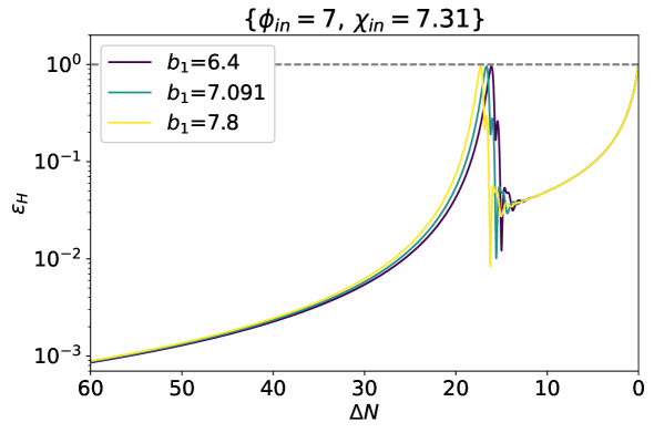
For appropriate choices of the model’s parameters, the background evolution of these models is characterised by two phases. The first is driven by the field , which slowly rolls down its potential while is effectively frozen due to the effect of the hyperbolic field-space geometry. When , the suppression is lifted, there is a turn in field space, and the second field starts rolling towards the minimum of its potential, up until the end of inflation [30]. At the transition between the two phases, and the (negative) term in eq.(2.14) causes a transient tachyonic instability for the entropic perturbation, which, as we have described, in turn sources a large on small scales [30].
In each model realisation, two parameters are particularly relevant, the value of , which determines the field-space curvature and therefore (roughly) the growth of , and the initial condition on the second field, , which sets the duration of the second phase of evolution and therefore the position of the peak in the scalar power spectrum [30].
In section 2.3 we investigate the effect that changes in have on the scalar power spectrum and non-Gaussianity, and do a similar analysis in appendix A for models where we vary . First, we present the background evolution for three working examples that we use throughout, namely three models with and different values of the geometrical parameter, .
2.3 Scalar non-Gaussianities
In this section, we calculate the scalar power spectrum and the primordial scalar non-Gaussianity, parametrised by the reduced bispectrum (2.11), for the working examples introduced in section 2.2. The numerical results presented in this section have been obtained using the publicly available code PyTransport [100, 89, 90]666See [101, 102, 103, 104, 105] for earlier related work, and [106, 107] for an alternative open source package, CppTransport, based on the same approach. PyTransport is available at github.com/jronayne/PyTransport.. The transport code works by evolving the 2- and 3-point function of covariant field fluctuations and their conjugate momenta from initial conditions set in the quantum regime on sub-horizon scales. It then converts these correlations into the power spectrum and bispectrum of [108].
An important quantity needed to connect inflationary dynamics with large-scale observables is the number of e-folds elapsed between the horizon crossing of the CMB scale, , and the end of inflation, defined as [1]
| (2.18) |
In this expression is the present comoving Hubble rate, is the energy density at the end of inflation, is the value of the potential when the comoving wavenumber crossed the horizon during inflation. The parameters and respectively represent the equation of state parameter during reheating and its duration
| (2.19) |
where is the energy scale at the end of it. For reheating to be completed before the onset of the Big Bang Nucleosynthesis [1], its duration is bounded from above:
| (2.20) |
When the equation-of-state parameter for reheating777For simplicity in the following we assume that . is , is maximised for instantaneous reheating, or . By assuming instant reheating and values of compatible with CMB observations, we iteratively solve eq.(2.18) for models with and , finding , regardless of . We also find that the maximum duration of reheating is . These quantities, together with the e-folding separation between the horizon crossing of the peak scale and the end of inflation, , determine the value of the scalar spectral tilt on large scales, see eq.(1.7). We approximate with the duration of the second phase of evolution, i.e. the number of e-folds that elapsed between the local maximum of and the end of inflation. We find that all the models we study are compatible at least at C.L. with the large-scale measurement (1.8) for appropriate choices of . For example, yields for the model with . We have also shown that for these models to be consistent with (1.8) at least at C.L., the inequality (1.11) follows, implying that viable models that satisfy constraints must lead to peaks in the scalar power spectrum beyond LISA scales, e.g. on scales relevant to LIGO or the Einstein telescope.
In [30] the authors fix , which would follow from . This value of , while being allowed by the upper bound , yields values of the scalar spectral tilt not compatible with (1.8). Nevertheless, in the following we will adopt for simplicity and consistency with [30]. This still serves as a useful benchmark to illustrate our conclusions regarding non-Gaussianity for these models, bearing in mind that while this choice leads to tensions with the measurements, there are appropriate choices of reheating duration (and therefore ) that make these models compatible with the Planck measurement (1.8), as explained above.
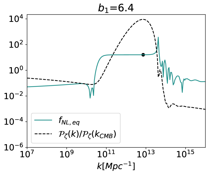
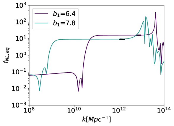
We display in figure 2 results for and the reduced bispectrum in the equilateral configuration, , at scales around the peak region for the three models introduced in section 2.2.
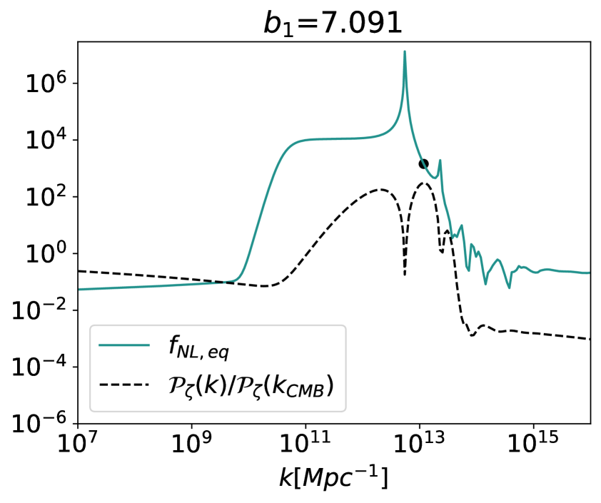
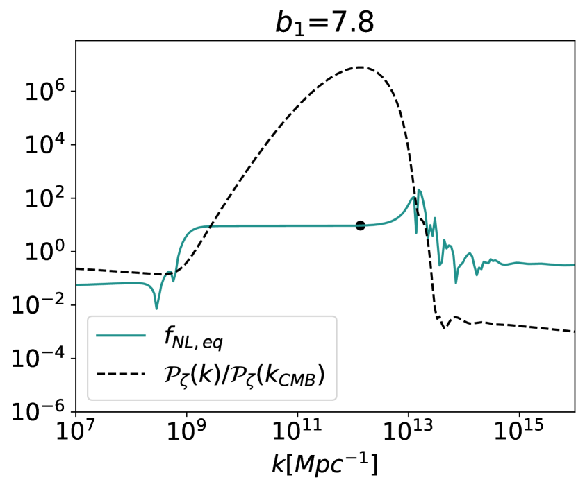
The enhancement of relative to the CMB scale is for each in increasing order. Interestingly the peak amplitude does not always increase for larger , i.e. more strongly-curved field spaces. We confirm this by systematically exploring more values in the range , see appendix B. In particular, figure 15 shows that for the peak amplitude starts decreasing up until the critical value , after which increases again for increasing . The presence of a critical value for the curvature divides the range into two regions, which motivates our choice of the three cases to work with.
In figure 2, we see that for and , is approximately flat, i.e. scale-independent, over the peak scales. However, for , which is close to the critical value, the scalar power spectrum exhibits a two-peak structure with the second peak being the largest, and the non-Gaussianity at is in a region of rapidly changing , outside of the plateau. As demonstrated in appendix B this is the exception, and all models with non-critical field-space curvature display a plateau in . We also find that the amplitude of the equilateral non-Gaussianity at the peak scale is non-monotonic for increasing , with for each in increasing order.
Excluding the critical value , the approximate scale-independence of the equilateral non-Gaussianity amplitude over peak scales points to non-Gaussianity of the local shape. We confirm this for the case by explicitly looking at the shape dependence of at fixed overall scale .
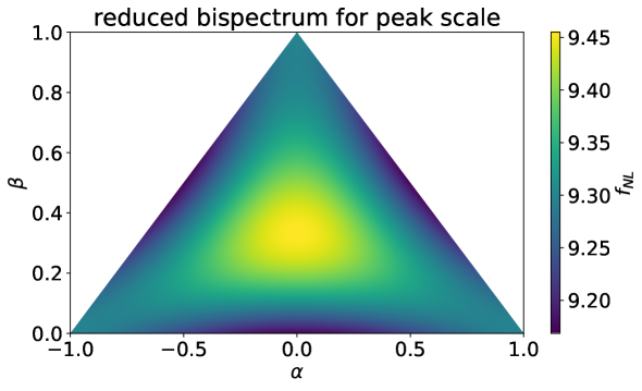
In figure 3 we display the reduced bispectrum as a function of , defined as , and . The range of values of the bispectrum shows that is almost constant for all triangle configurations, meaning that the bispectrum is scale-independent and therefore of the local shape. We have checked that as we increase the resolution of the triangle plot, i.e. the closer we get to the squeezed configuration represented by the triangle points , we see a drop in the value of , which is expected since does eventually display a scale dependence at scales outside of the plateau.
3 Calculating non-Gaussianities: the numerical approach
When non-Gaussianity is local, it is highly suggestive that it has been produced on super-horizon scales. In order to test this hypothesis, and to cross check the results obtained in section 2, we develop here a second numerical approach, based on the formalism [109, 110, 111, 112, 113].
The formalism is a powerful tool to compute the non-linear evolution of cosmological perturbations on large scales, . In particular, the curvature perturbation is identified with the perturbed number of e-folds of evolution between a spatially-flat hypersurface at time and a uniform-density hypersurface at time
| (3.1) |
where . By Taylor expanding eq.(3.1) for two fields and by retaining only linear contributions888We have checked that truncating the expansion at the linear order is sufficient to justify the results obtained in section 2, see e.g. figure 5., we get
| (3.2) |
Eq.(3.2) can be used to calculate the scalar power spectrum
| (3.3) |
where and . For each scale the 2-point correlators appearing in eq.(3.3) are evaluated at horizon crossing, and the formalism takes into account all the subsequent (and possibly complicated) evolution to produce the curvature power spectrum.
We apply eq.(3.3) to calculate super-horizon contributions to the scalar power spectrum and primordial scalar non-Gaussianities in the models analysed in section 2. For this purpose, we calculate in appendix C analytic expressions for the correlators appearing in (3.3), which need to be evaluated at horizon crossing. In particular, we employ the mode functions for non-interacting, massless fields in a quasi-de Sitter background, see eq.(C.1).
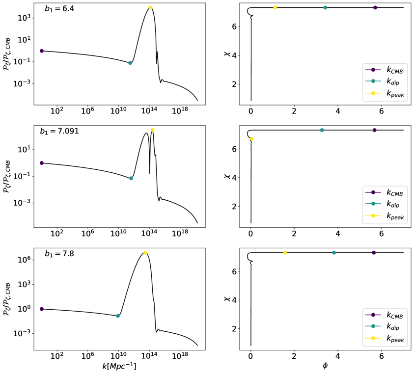
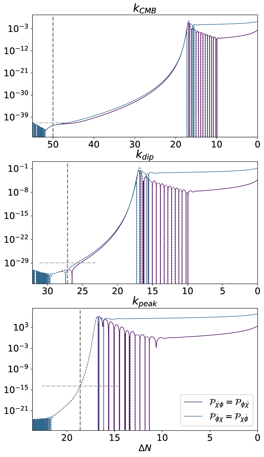
For the models with and , the peak scale leaves the horizon before the turn in field space (e.g. before the isocurvature perturbation becomes unstable), see figure 4. Here we represent on the left , with the CMB, dip and peak scales highlighted, and mark on the right the times at which these scales cross the horizon on top of the fields’ evolution. In both cases, the peak scale leaves the horizon before the field-space trajectory turns and for this reason we expect our approach, that relies on the correlator (C.1), to well describe the perturbations in the peak region. When , the scalar power spectrum exhibits a double peak, with the second peak larger than the first one and the peak scale exiting the horizon during the transition. For critical curvature values, , we therefore expect sub-horizon effects to be relevant. This implies that correlators at horizon crossing receive corrections from sub-horizon interactions, and using the correlators for non-interacting, massless fields on de Sitter, eq.(C.1), is only appropriate as a first approximation. In this (exceptional) case we therefore expect our approach not to fully account for the perturbations evolution.
By using the results of appendix C, eq.(3.3) reduces to
| (3.4) |
where the dimensionless correlators are listed in eqs.(C.23)-(C.32) and need to be evaluated for each scale at horizon crossing.
3.1 The scalar power spectrum
With , we adjust in eq.(2.17) such that the scalar power spectrum amplitude on large scales satisfies the Planck normalisation [1]. We numerically solve the background evolution with initial conditions 999We have chosen the initial condition such that inflation lasts longer than and the background trajectory is on the slow-roll attractor when the CMB scale crossed the horizon. and stop the evolution when : the resulting set of numerical solutions constitutes our reference background evolution. The energy density at the end of inflation for the solutions , , defines a constant-energy-density hypersurface, which will be our reference when calculating (3.1).
We slice the time-evolution during the observable window of inflation by considering equally spaced e-folding numbers, , each of which is associated with a comoving scale, , that crossed the horizon at that time
| (3.5) |
where we have assumed and is defined in eq.(2.18). Using , we evaluate for each the corresponding set , which can be regarded as the set of initial conditions at the time of horizon crossing of the scale . For each , we evaluate the analytic expressions for the 2-point correlators in eq.(3.4), see appendix C, at horizon crossing by using the set . The correlators values will be used in evaluating eq.(3.4) for each scale .
We calculate the derivatives in (3.4) in the same way, so we describe in detail just one of the cases, . For each time , we consider the reference set of initial conditions and vary only the initial condition for ,
| (3.6) |
In particular, we consider 61 new initial conditions, with . For each one of these, which we label with the perturbed value , where , we solve the background evolution up until and evaluate the number of e-folds this takes, . We then fit the obtained numerical data with the linear function
| (3.7) |
and identify for the scale . The product of the square with the value of the 2-point correlator at horizon crossing constitutes the first contribution to (3.4) for the scale . We repeat the same procedure for the remaining initial conditions in to derive and . By using these results, the correlators at horizon crossing in eqs.(C.23)-(C.32), and eq.(3.4), we obtain . Repeating this for all the scales yields to the numerical result for the scalar power spectrum.
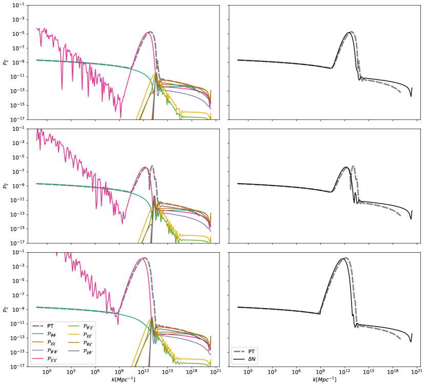
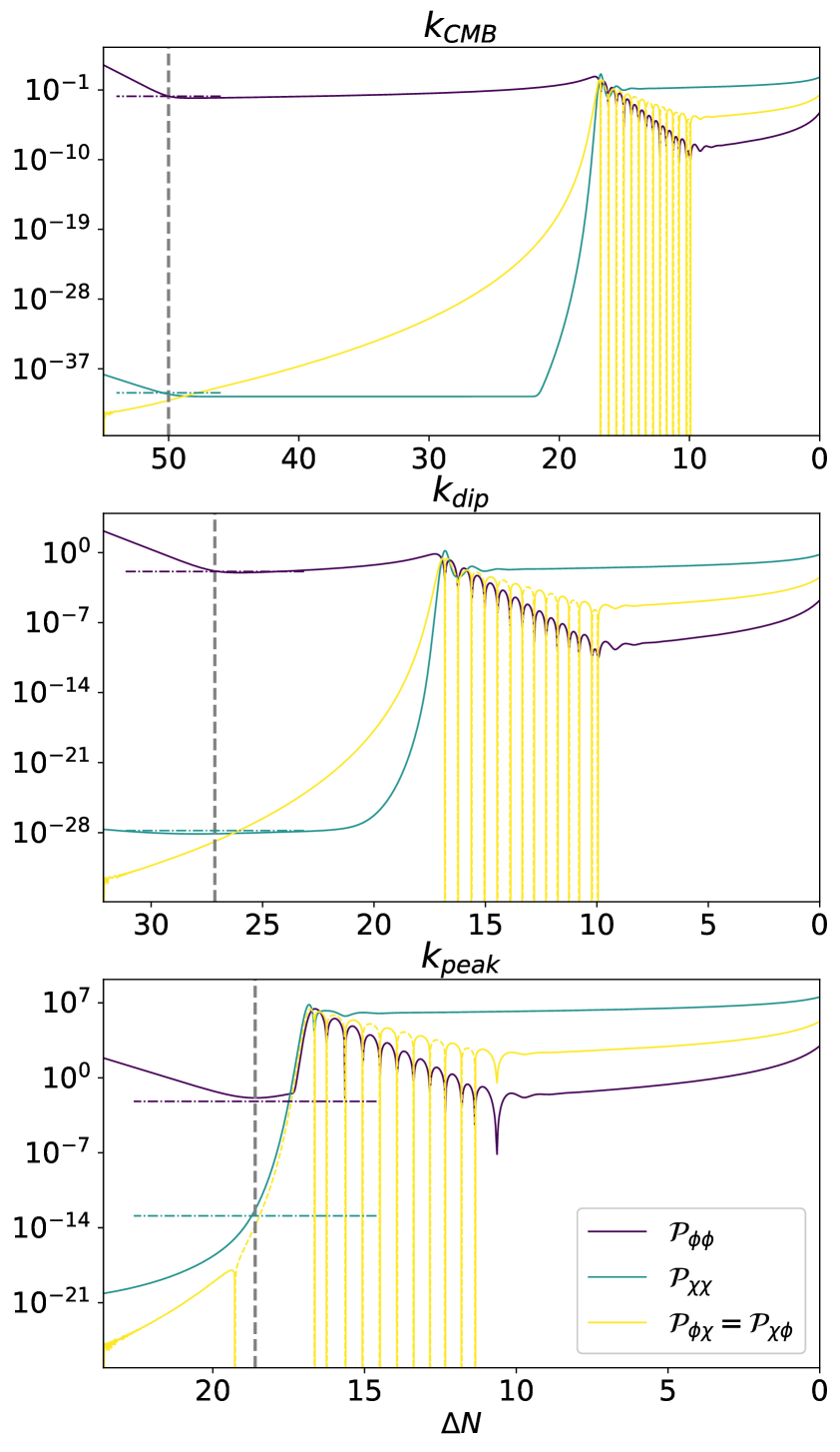
We represent in the left panels of figure 5 the results obtained for models with different values of . In particular, the colored lines represent the eight contributions to the scalar power spectrum within the numerical calculation, see eq.(3.4), and the gray-dashed line displays the PyTransport result for comparison.
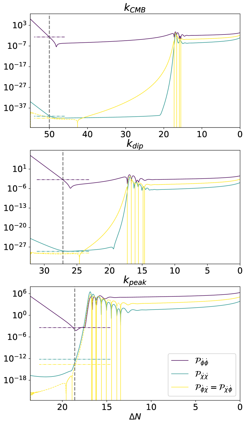
In each case the power spectrum is first dominated by perturbations in the field, which at these times is slowly rolling, while is frozen. The peak is produced by perturbations in the second field velocity, . On large scales, the contribution is dominated by numerical noise101010The unstable quantity here is , which rapidly oscillates between large positive and negative values, see figure 6. The information on the sign of is lost in figure 5, due to the square taken, see eq.(3.4).. This is easily explained considering the fact that during the first stage of evolution is frozen, with exponentially suppressed, and dealing with such extreme values leads to some instabilities in the numerics. The numerical peak is slightly different with respect to the PyTransport result, especially when considering its position. This is probably due to the analytic correlators that we use to implement the calculation, which rely on a series of approximations, see eq.(C.1).
After the peak region, the scalar power spectrum displays a second slow-roll plateau. The largest contribution at these scales is given by fluctuations in , which is slowly rolling and dominates the second phase of evolution after the transition. Comparable to this contribution are those of mixed cross-correlators, and . The sum of all contributions yields a plateau slightly larger than the PyTransport one, see the right panels in figure 5, where we compare the sum111111On large scales we neglect the noise-dominated contribution. of the eight contributions, see eq.(3.4), with the PyTransport results. The discrepancy between the two approaches increases towards smaller scales. These differences might be explained by the fact that small scales cross the horizon towards the end of inflation, where the slow-roll approximation fails, and our initial conditions for the formalism are no longer appropriate.
While the agreement between the numerical results and the output of PyTransport is quite remarkable for and , in the case of the fluctuations in explain only the first (secondary) peak in the scalar power spectrum. This is not surprising considering the fact that the peak scale crossed the horizon during the turn in field space, see figure 4, signalling that sub-horizon effects (not accounted for by our analytic correlators at horizon crossing) need to be taken into account.
As discussed in section 2.3, the PyTransport results show a critical behavior in the scalar power spectrum for , see also figure 14. We find a sign of criticality also in quantities calculated with the approach.
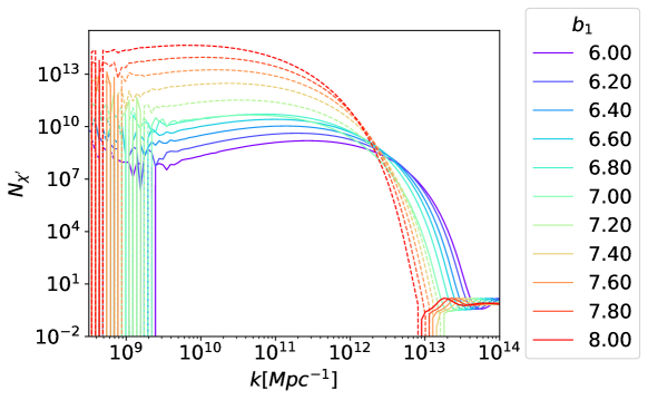
We display in figure 6 values of for scales in the peak region for different values of . We distinguish positive (continuous) and negative (dashed) values of . The transition between positive and negative in the peak region is located between and , exactly where expected from the PyTransport results. This flags with a second independent approach the presence of critical values for the geometrical parameter around .
3.2 Scalar non-Gaussianities
The amplitude of scalar non-Gaussianities (more precisely the shape-independent part of ) can be calculated within the formalism as (see e.g. [114, 115])
| (3.8) |
where . In section 3.1 we have demonstrated that the peak in the scalar power spectrum is due to fluctuations in the second field velocity, . For this reason we expect the amplitude of non-Gaussianity around the scale to be approximately given as
| (3.9) |
Since the numerical approach does not reproduce the position of the peak in the scalar power spectrum precisely, see figure 5, we use the numerical results from PyTransport to derive the peak position, . We select 10 scales that crossed the horizon around the same time as , in the range
| (3.10) |
For each of these scales, we use the reference background evolution to calculate the initial conditions at horizon crossing, , and consider a small variation of the initial condition for the velocity ,
| (3.11) |
Following a procedure similar to what described in section 3.1, we derive the numerical data and obtain the derivatives and by using a linear and quadratic fit respectively to the data. We then combine these derivatives for each scale as prescribed by eq.(3.9).
We represent the results for our two121212We do not expect the numerical approach to yield the correct for the model with as we have already seen that it fails at reproducing the principal peak in , see the central panel in figure 5. working examples with and in figure 7. For comparison, we show the numerical values together with the PyTransport results. The non-Gaussianity amplitudes for scales around calculated with the two different numerical approaches agree to a very good level.
4 The field-space geometry, non-Gaussianity and perturbativity
In section 2, we calculated with PyTransport the amplitude of non-Gaussianity associated with large peaks in the scalar power spectrum for models of [30, 32] with different values of the field-space curvature. In section 3 we have validated the results of section 2 by means of a second numerical approach, based on the formalism. Here, we explore in more detail the dependence of the amplitude of non-Gaussianity at peak scales on the geometrical parameter , and use the results to assess the perturbativity of these models.
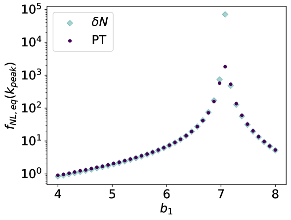
We display in figure 8 at for models with different values of (for more details see appendix B). By comparing the PyTransport and numerical results, we see that overall the two series of points agree quite well, with deviations for cases with . These are expected considering the fact that crossed the horizon during the turn in field space for these models (see figure 4) and sub-horzion effects, not captured by the analytic correlators at horizon crossing that we use, are therefore expected to be relevant. The amplitude increases in magnitude for increasing , with a faster and faster rate, peaks for and then decreases again for the remaining range of . As is the case for the power spectrum amplitude at , see figure 15, the amplitude of non-Gaussianity also displays a critical behavior at .
As shown in section 2, the non-Gaussianity at peak scales is approximately of the local type for models with different from the critical value. For local non-Gaussianity, when one field or field velocity perturbation at horizon crossing is the dominant contribution to (as is the case here), the curvature perturbation in real space can be expanded as (see for example [116])131313See [117] for a calculation including the cubic non-Gaussianity parameter.
| (4.1) |
where is the Gaussian contribution to the curvature perturbation and is its variance. Beginning from eq.(4.1) and moving to Fourier space, we find that
| (4.2) |
where is an infrared cutoff and the Gaussian power spectrum that comes from including only the leading term in eq.(4.1). When the Gaussian power spectrum is scale invariant, the integral above can be performed exactly (see for example [118, 119]), and the ratio between the one-loop power spectrum and the Gaussian one is
| (4.3) |
One can take to be the scale over which the power spectrum is being measured, and hence can be taken to be close to for our purposes, such that . Given our power-spectrum is not scale invariant over the peak scales, this expression can only be taken as an indication of when perturbativity breaks down. By requiring , eq.(4.3) yields
| (4.4) |
which we will use in the following as a criterion to assess the perturbativity of these models, given the amplitude of the scalar power spectrum and non-Gaussianity at the peak scales. Note that (4.4) is an upper limit, and perturbativity, or least the accuracy of results, may be in question well before the bound is saturated.
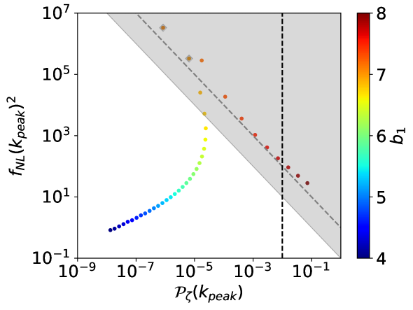
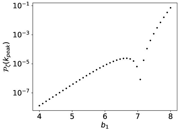
In figure 9 we represent against for the same models considered in figure 8. The gray area highlights regions for which , which according to (4.4) signals a breakdown of perturbativity. The points highlighted with a gray diamond correspond to models with critical values of the field-space curvature, therefore we should not apply the criterion (4.4), valid for local non-Gaussianity, to these points. With these points excluded, all models with violate (4.4). In particular, models that could lead to PBH production (the usual criteria is for Gaussian perturbations which drops to when the smoothed density contrast, rather than , is used to calculate the abundance of PBHs [120]) and/or large second-order GWs are all flawed by perturbativity issues.
Figure 9 illustrates again the fact that the peak amplitude does not always increase by increasing the value of the geometrical parameter, as well as how behaves. This has important consequences for power spectra with smaller peaks, : they can produced within models with different values of , but each model corresponds to a different non-Gaussianity amplitude, some of which violate the criterion (4.4).
5 Discussion
In this work we have investigated multi-fields models of inflation with hyperbolic field space. We focus on the polynomial -attractors introduced in [30], which can deliver a large peak in the scalar power spectrum on small scales due to geometrical destabilisation and turning trajectories. In some cases the scalar power spectrum could lead to large second-order GWs and possibly result into PBH production. We show that peaks at scales are consistent at least at C.L. with large-scale measurements of the scalar spectral tilt, and therefore these models could provide a relevant source to the stochastic background of GWs at interferometer scales, and deserve further investigation.
Up to now the models of [30], and other similar ones where multi-field effects are responsible for the peak in (see e.g. [29, 28, 31]) have been investigated only at the linear level, i.e. by employing the linear equations of motion for the perturbations. In this work we make a step towards investigating non-linear effects, and calculate the scalar bispectrum at peak scales. We find that the amplitude of non-Gaussianity, as well as the scalar power spectrum peak, depends non-monotonically on the field-space curvature and on the initial condition for the second field, which encourages us to identify critical values for these parameters. For models with non-critical values of the parameters, we show that the peak in the scalar power spectrum results from super-horizon effects and that the scalar non-Gaussianity is of the local type at peak scales, with a plateau region highly reminiscent of that found in single-field models (see e.g. [64]). This is an important result since the effect of non-Gaussianity on gravitational wave production has been investigated in detail only for local non-Gaussianity. Our result indicates that the framework of, e.g., [72], which is based on local non-Gaussianity, can immediately be applied to models such as the one studied here, at least as a first approximation.
We derive and cross check our results by employing two different numerical tools, the code PyTransport and a newly developed approach based on the formalism, whose applicability is due to the super-horizon evolution of peak-scales modes. The numerical results allow us to also establish that the scalar power spectrum peak originates from fluctuations in the second field velocity.
We employ our results to assess the perturbativity of these models. Since the non-Gaussianity is approximately local, we use as a diagnostic tool the quantity and find that many realisations of these models are flawed by perturbativity issues, including phenomenologically-interesting cases with large peaks in the scalar power spectrum, , see figures 9 and 13. To our knowledge this work provides the first attempt to assess the perturbativity of a multi-field model with a peak in the scalar power spectrum.
Non-Gaussianity arising in two-field models of inflation with hyperbolic field space and non-geodesic motion has been the subject of several investigations [98, 121, 122, 123, 124]141414For recent efforts in computing non-Gaussianity in multi-field models within the cosmological bootstrap program see e.g. [125], and [126] for the cosmological flow framework.. Previous studies address models where the entropic perturbation instability is triggered on sub-horizon scales151515More recently, super-horizon effects are taken into account by means of an analytical calculation, showing that rapidly turning trajectories can produce potentially large bispectra, with contributions from many shapes [127]. and the curvature perturbation exponentially grows around horizon crossing, getting amplified at all scales; for these models the non-Gaussianity is enhanced in the flattend configuration. As discussed above, in this work we consider a different class of models, focusing on hyperbolic models delivering amplified scalar fluctuations on small scales.
There are many possible directions for future work. Similarly to what has been done for single-field models leading to enhanced fluctuations [75, 76, 77, 80, 81, 79, 82, 83], one could check the viability of multi-field models by calculating the one-loop correction to the tree-level scalar power spectrum. Note that this approach does not rely on the assumption of the non-Gaussianity being of the local type. We also plan to expand on these results by comparing them with the non-Gaussianity produced within multi-field models where the peak is produced from sub-horizon effects. In addition, it would be interesting to understand why, for the models considered in this work, sub-horizon effects become relevant for critical values of the field-space curvature and initial conditions.
We conclude by noting that there are two important lessons to draw from our work, which likely extend to other models. First, non-Gaussianity can be large over peak scales, potentially leading to important effects in PBH formation rates, and in the spectrum of scalar induced gravitational waves. Secondly, non-Gaussianity can potentially be too large for strongly curved field space metrics, which at a minimum renders perturbative calculations invalid in this regime.
Acknowledgments
The authors would like to thank David Wands for many interesting discussions on related topics and for very useful comments on the manuscript. DJM is supported by a Royal Society University Research Fellowship and LI by a Royal Society funded postdoctoral position.
Appendix A Varying
We illustrate here the impact that changes in the initial condition of the second field, , have on the scalar power spectrum and non-Gaussianity. We consider models with and (chosen such that the scalar power spectrum reaches at LIGO scales), and vary .
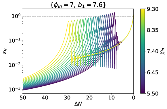
In figure 10 the time-dependence of shows two phases of inflation, separated by a transition with , with the duration of the second phase of evolution, which is driven by , set by the value of . We note that the exact value of at the transition also depends on , and for some models inflation is briefly interrupted.
The duration of the second phase of evolution is important in determining the value of the scalar spectral tilt on large scales. This is shown in eq.(1.7), where we can approximate with the duration of the second phase. Assuming instant reheating, we iteratively solve eq.(2.18) with values compatible with Planck measurements of the amplitude of scalar perturbations and find for these models. We also find that the maximum allowed duration of reheating, see eq.(2.20), is . These models are compatible at least at C.L. with (1.8) for initial conditions and appropriate choices of , with larger corresponding to shorter reheating stages. We also find that initial conditions could yield a peak in the scalar power spectrum at ET or LIGO scales, whilst complying with (1.8) at least at C.L.. By using eq.(2.18), it is easy to show that (used in [30]) is not compatible with the values obtained for and . Nevertheless, constraining the parameter space of these models in view of the compatibility with large-scale measurements is not the focus of this work, so we will employ here, as was used in [30] and in the main body of the paper for the set of models where we varied .
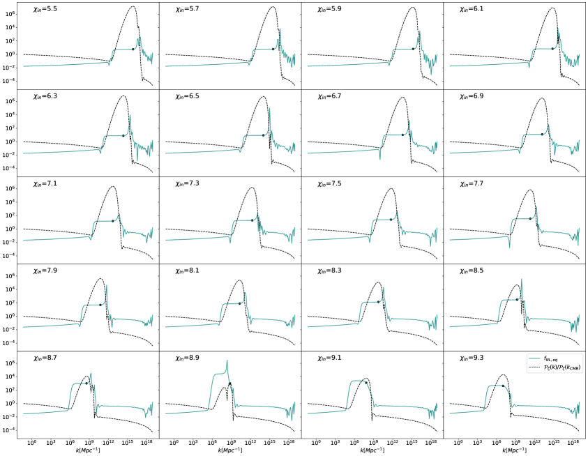
We display in figure 11 results for and the reduced bispectrum in the equilateral configuration, , at scales around the peak region for the same models of figure 10. For larger the second phase of background evolution lasts longer, see figure 10, which explains why the peak is located on larger scales. The peak region is characterised by an almost flat profile for , as for the models analysed in section 2, hinting at non-Gaussianity of the local type. This is true for all cases except for , where is outside of the plateau region, in a zone of rapidly varying . Also note that in this case the scalar power spectrum exhibits a two-peak structure, with the second peak being the largest.
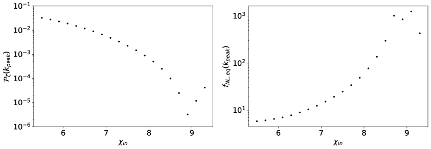
Considering this and the behavior of and against , see figure 12, we conclude that models in which is varied also display signs of criticality.
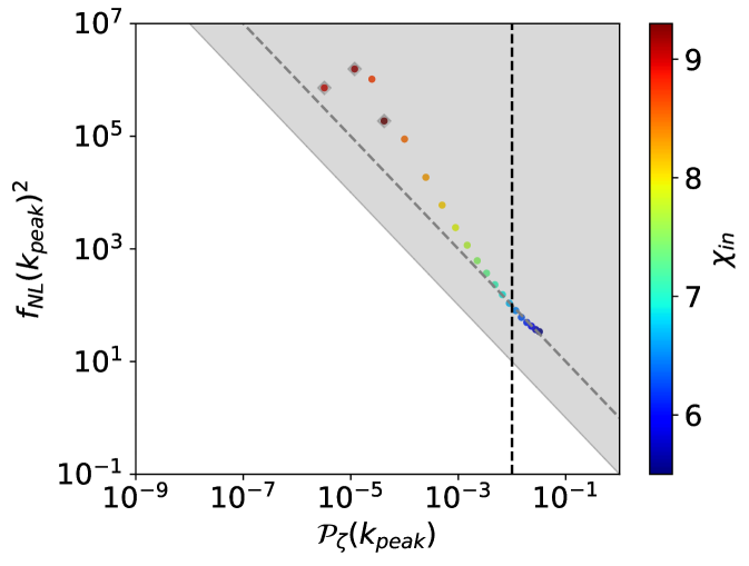
Similarly to what has been done for the set of models where we varied , see figure 9, we display in figure 13 values of against . The points highlighted with gray diamonds correspond to critical values of , in which case the non-Gaussianity is not of the local type. For all the other models, the criterion (4.4) applies and figure 13 shows that they are all flawed by perturbativity issues, including those delivering a large peak at LIGO and ET scales.
Appendix B Varying
To motivate our choice of values for the field-space geometrical parameter in section 2, we include here results for the scalar power spectrum and amplitude of equilateral non-Gaussianity derived for additional values in the range .
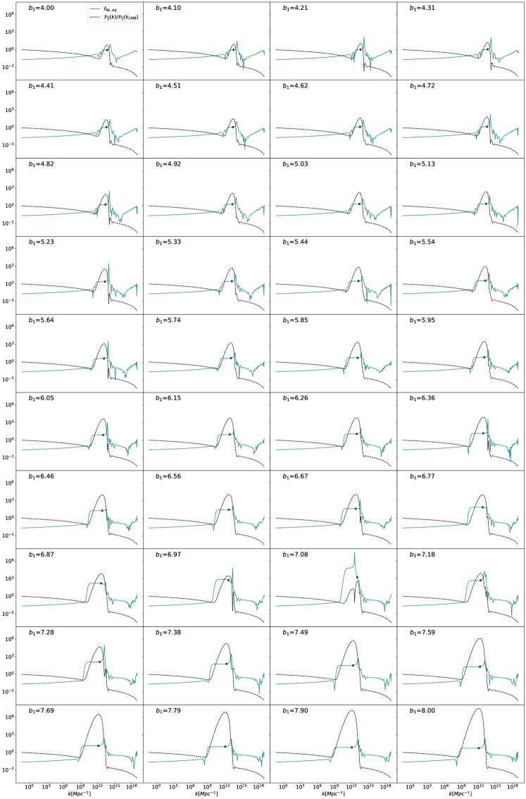
We display in figure 14 numerical results for and , calculated using PyTransport, for 40 values of . When , the scalar power spectrum is characterised by a two-peak structure, with the second peak being also the principal one. Also, while in all the other cases (black dots in figure 14) lies in the plateau region, for this is not true.
We show in figure 15 values of against , which clearly display a non-monotonic behavior.
The results represented in figures 14 and 15 show a change of behavior for the power spectrum and equilateral non-Gaussianity amplitudes at the peak scale when . For this reason, in section 2 we choose to discuss the three values , respectively smaller than, similar to and larger than the critical value.
Appendix C Analytic 2-point correlators at horizon crossing
Here we derive expressions for the 2-point correlation function of the fields and their velocities used in the numerical computation described in section 3. In particular, we follow the approach of [100].
Assuming that the fields are massless and non-interacting at the time in which to evaluate the 2-point correlators, i.e. at horizon crossing, the 2-point correlator at unequal times in nearly de Sitter spacetime reads161616Besides requiring the fields to be non-interacting and effectively massless, eq.(C.1) also relies on the slow-roll approximation, . This holds if the scales of interest exit the horizon before the turn in field space, which is true for peak scales in all the field-space curvature cases considered, except for the critical values , see section 3.
| (C.1) |
where we use conformal time, . At linear-order stands for the field perturbation, with the indices such that, e.g., . In eq.(C.1), is defined as [128]
| (C.2) |
where we have defined the exponential operator and given the first three terms of its Taylor expansion. Eq.(C.2) shows that in the limit , and therefore coincides with .
Using (C.1) and (C.2), it is straightforward to show that the fields 2-point correlator at equal times is given by
| (C.3) |
In order to derive correlators involving field velocities, it is useful to first calculate derivatives of with respect to and . By using eq.(C.2) and applying the Leibniz integral rule, we obtain
| (C.4) | ||||
| (C.5) |
and
| (C.6) |
By taking the limit , eqs.(C.4)-(C.6) reduce to
| (C.7) | ||||
| (C.8) | ||||
| (C.9) |
By using eq.(C.1) and eqs.(C.7)-(C.9), one can then derive the equal-times field-velocity cross-correlators
| (C.10) |
| (C.11) |
and the equal-times velocity-velocity correlators
| (C.12) |
Note that in deriving eqs.(C.10)-(C.12), we do not take time-derivatives of the Hubble rate since eq.(C.1) relies on the slow-roll approximation, .
For the purpose of the numerical calculation of section 3, we need the time-derivatives of the fields to be calculated with respect to , where . Note that the prime symbol stands for a derivative with respect to . Also, on de Sitter . By keeping this into account and using the metric (2.15) and the Christoffel symbols (2.16) in eqs.(C.3), (C.10)-(C.12), we get
| (C.13) | ||||
| (C.14) | ||||
| (C.15) | ||||
| (C.16) | ||||
| (C.17) | ||||
| (C.18) | ||||
| (C.19) | ||||
| (C.20) | ||||
| (C.21) | ||||
| (C.22) |
where we simplify the notation by defining the dimensionless power spectrum .
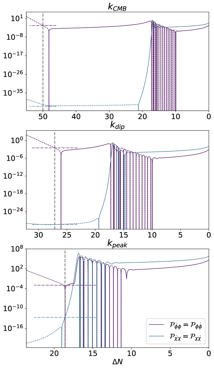
In figures 16 and 17 we provide an explicit check of the expressions derived above. For this purpose we transform derivatives with respect to into derivatives with respect to cosmic time . We compare the numerical evolution of each correlator, calculated with PyTransport, with the corresponding dot-dashed line, representing the analytic expressions derived above evaluated at horizon crossing (). If two correlators are equal numerically, e.g. and , we only represent one of the two. In the left panel of figure 16 there is no line corresponding to the analytic correlator because it is zero according to the corresponding analytic expression (C.15), due to the fact that the metric is diagonal. Figures 16 and 17 show that the analytical correlators match remarkably well the numerical values at horizon crossing in most cases, with slight deviations for the mixed field-velocity cross-correlators, see the right panel of figure 17.
In eqs.(C.13)-(C.22), the leading terms in the limit represent the homogeneous growing mode, to be used in the calculation, while terms proportional to constitute gradient corrections. By retaining only the homogeneous growing mode, the 2-point correlators at horizon crossing are
| (C.23) | ||||
| (C.24) | ||||
| (C.25) | ||||
| (C.26) |
| (C.27) | |||
| (C.28) | |||
| (C.29) | |||
| (C.30) | |||
| (C.31) |
| (C.32) |
where the time-dependent functions appearing in these expressions are to be evaluated at horizon crossing, . These correlators represent the initial conditions for the calculation of section 3.
References
- [1] Planck collaboration, Planck 2018 results. X. Constraints on inflation, Astron. Astrophys. 641 (2020) A10 [1807.06211].
- [2] B. J. Carr and S. W. Hawking, Black Holes in the Early Universe, Monthly Notices of the Royal Astronomical Society 168 (1974) 399.
- [3] M. Sasaki, T. Suyama, T. Tanaka and S. Yokoyama, Primordial black holes—perspectives in gravitational wave astronomy, Class. Quant. Grav. 35 (2018) 063001 [1801.05235].
- [4] B. Carr, K. Kohri, Y. Sendouda and J. Yokoyama, Constraints on primordial black holes, Rept. Prog. Phys. 84 (2021) 116902 [2002.12778].
- [5] S. Bird, I. Cholis, J. B. Muñoz, Y. Ali-Haïmoud, M. Kamionkowski, E. D. Kovetz et al., Did LIGO detect dark matter?, Phys. Rev. Lett. 116 (2016) 201301 [1603.00464].
- [6] G. Bertone and T. Tait, M. P., A new era in the search for dark matter, Nature 562 (2018) 51 [1810.01668].
- [7] N. Bartolo, V. De Luca, G. Franciolini, A. Lewis, M. Peloso and A. Riotto, Primordial Black Hole Dark Matter: LISA Serendipity, Phys. Rev. Lett. 122 (2019) 211301 [1810.12218].
- [8] K. N. Ananda, C. Clarkson and D. Wands, The Cosmological gravitational wave background from primordial density perturbations, Phys. Rev. D 75 (2007) 123518 [gr-qc/0612013].
- [9] D. Baumann, P. J. Steinhardt, K. Takahashi and K. Ichiki, Gravitational Wave Spectrum Induced by Primordial Scalar Perturbations, Phys. Rev. D 76 (2007) 084019 [hep-th/0703290].
- [10] R. Saito, J. Yokoyama and R. Nagata, Single-field inflation, anomalous enhancement of superhorizon fluctuations, and non-Gaussianity in primordial black hole formation, JCAP 06 (2008) 024 [0804.3470].
- [11] R. Saito and J. Yokoyama, Gravitational-Wave Constraints on the Abundance of Primordial Black Holes, Prog. Theor. Phys. 123 (2010) 867 [0912.5317].
- [12] J. Fumagalli, S. Renaux-Petel and L. T. Witkowski, Resonant features in the stochastic gravitational wave background, 2105.06481.
- [13] L. T. Witkowski, G. Domènech, J. Fumagalli and S. Renaux-Petel, Expansion history-dependent oscillations in the scalar-induced gravitational wave background, 2110.09480.
- [14] M. Braglia, X. Chen and D. K. Hazra, Probing Primordial Features with the Stochastic Gravitational Wave Background, JCAP 03 (2021) 005 [2012.05821].
- [15] H. Motohashi and W. Hu, Primordial Black Holes and Slow-Roll Violation, Phys. Rev. D 96 (2017) 063503 [1706.06784].
- [16] J. Garcia-Bellido and E. Ruiz Morales, Primordial black holes from single field models of inflation, Phys. Dark Univ. 18 (2017) 47 [1702.03901].
- [17] C. Germani and T. Prokopec, On primordial black holes from an inflection point, Phys. Dark Univ. 18 (2017) 6 [1706.04226].
- [18] G. Ballesteros and M. Taoso, Primordial black hole dark matter from single field inflation, Phys. Rev. D 97 (2018) 023501 [1709.05565].
- [19] M. Cicoli, V. A. Diaz and F. G. Pedro, Primordial Black Holes from String Inflation, JCAP 06 (2018) 034 [1803.02837].
- [20] I. Dalianis, A. Kehagias and G. Tringas, Primordial black holes from -attractors, JCAP 01 (2019) 037 [1805.09483].
- [21] S. Passaglia, W. Hu and H. Motohashi, Primordial black holes and local non-Gaussianity in canonical inflation, Phys. Rev. D 99 (2019) 043536 [1812.08243].
- [22] N. Bhaumik and R. K. Jain, Primordial black holes dark matter from inflection point models of inflation and the effects of reheating, JCAP 01 (2020) 037 [1907.04125].
- [23] S. Balaji, J. Silk and Y.-P. Wu, Induced gravitational waves from the cosmic coincidence, JCAP 06 (2022) 008 [2202.00700].
- [24] H. V. Ragavendra and L. Sriramkumar, Observational Imprints of Enhanced Scalar Power on Small Scales in Ultra Slow Roll Inflation and Associated Non-Gaussianities, Galaxies 11 (2023) 34 [2301.08887].
- [25] S. R. Geller, W. Qin, E. McDonough and D. I. Kaiser, Primordial black holes from multifield inflation with nonminimal couplings, Phys. Rev. D 106 (2022) 063535 [2205.04471].
- [26] W. Qin, S. R. Geller, S. Balaji, E. McDonough and D. I. Kaiser, Planck Constraints and Gravitational Wave Forecasts for Primordial Black Hole Dark Matter Seeded by Multifield Inflation, 2303.02168.
- [27] D. Baumann and L. McAllister, Inflation and String Theory, Cambridge Monographs on Mathematical Physics. Cambridge University Press, 2015, 10.1017/CBO9781316105733, [1404.2601].
- [28] J. Fumagalli, S. Renaux-Petel, J. W. Ronayne and L. T. Witkowski, Turning in the landscape: a new mechanism for generating Primordial Black Holes, 2004.08369.
- [29] G. A. Palma, S. Sypsas and C. Zenteno, Seeding primordial black holes in multifield inflation, Phys. Rev. Lett. 125 (2020) 121301 [2004.06106].
- [30] M. Braglia, D. K. Hazra, F. Finelli, G. F. Smoot, L. Sriramkumar and A. A. Starobinsky, Generating PBHs and small-scale GWs in two-field models of inflation, JCAP 08 (2020) 001 [2005.02895].
- [31] L. Iacconi, H. Assadullahi, M. Fasiello and D. Wands, Revisiting small-scale fluctuations in -attractor models of inflation, JCAP 06 (2022) 007 [2112.05092].
- [32] R. Kallosh and A. Linde, Dilaton-axion inflation with PBHs and GWs, JCAP 08 (2022) 037 [2203.10437].
- [33] M. Braglia, A. Linde, R. Kallosh and F. Finelli, Hybrid -attractors, primordial black holes and gravitational wave backgrounds, 2211.14262.
- [34] R. Kallosh and A. Linde, Universality Class in Conformal Inflation, JCAP 07 (2013) 002 [1306.5220].
- [35] R. Kallosh and A. Linde, Multi-field Conformal Cosmological Attractors, JCAP 12 (2013) 006 [1309.2015].
- [36] S. Ferrara, R. Kallosh, A. Linde and M. Porrati, Minimal Supergravity Models of Inflation, Phys. Rev. D 88 (2013) 085038 [1307.7696].
- [37] R. Kallosh and A. Linde, Superconformal generalization of the chaotic inflation model , JCAP 06 (2013) 027 [1306.3211].
- [38] R. Kallosh and A. Linde, Superconformal generalizations of the Starobinsky model, JCAP 06 (2013) 028 [1306.3214].
- [39] R. Kallosh and A. Linde, Non-minimal Inflationary Attractors, JCAP 10 (2013) 033 [1307.7938].
- [40] R. Kallosh, A. Linde and D. Roest, Universal Attractor for Inflation at Strong Coupling, Phys. Rev. Lett. 112 (2014) 011303 [1310.3950].
- [41] R. Kallosh, A. Linde and D. Roest, Superconformal Inflationary -Attractors, JHEP 11 (2013) 198 [1311.0472].
- [42] R. Kallosh and A. Linde, Escher in the Sky, Comptes Rendus Physique 16 (2015) 914 [1503.06785].
- [43] J. J. M. Carrasco, R. Kallosh, A. Linde and D. Roest, Hyperbolic geometry of cosmological attractors, Phys. Rev. D 92 (2015) 041301 [1504.05557].
- [44] M. Galante, R. Kallosh, A. Linde and D. Roest, Unity of Cosmological Inflation Attractors, Phys. Rev. Lett. 114 (2015) 141302 [1412.3797].
- [45] J. Fumagalli, Renormalization Group independence of Cosmological Attractors, Phys. Lett. B 769 (2017) 451 [1611.04997].
- [46] R. Kallosh and A. Linde, Polynomial -attractors, JCAP 04 (2022) 017 [2202.06492].
- [47] A. R. Brown, Hyperbolic Inflation, Phys. Rev. Lett. 121 (2018) 251601 [1705.03023].
- [48] S. Mizuno and S. Mukohyama, Primordial perturbations from inflation with a hyperbolic field-space, Phys. Rev. D 96 (2017) 103533 [1707.05125].
- [49] A. Achúcarro, R. Kallosh, A. Linde, D.-G. Wang and Y. Welling, Universality of multi-field -attractors, JCAP 04 (2018) 028 [1711.09478].
- [50] A. Linde, D.-G. Wang, Y. Welling, Y. Yamada and A. Achúcarro, Hypernatural inflation, JCAP 07 (2018) 035 [1803.09911].
- [51] P. Christodoulidis, D. Roest and E. I. Sfakianakis, Angular inflation in multi-field -attractors, JCAP 11 (2019) 002 [1803.09841].
- [52] J. S. Bullock and J. R. Primack, NonGaussian fluctuations and primordial black holes from inflation, Phys. Rev. D 55 (1997) 7423 [astro-ph/9611106].
- [53] J. Yokoyama, Chaotic new inflation and formation of primordial black holes, Phys. Rev. D 58 (1998) 083510 [astro-ph/9802357].
- [54] C. T. Byrnes, E. J. Copeland and A. M. Green, Primordial black holes as a tool for constraining non-Gaussianity, Phys. Rev. D 86 (2012) 043512 [1206.4188].
- [55] S. Young and C. T. Byrnes, Primordial black holes in non-Gaussian regimes, JCAP 08 (2013) 052 [1307.4995].
- [56] E. V. Bugaev and P. A. Klimai, Primordial black hole constraints for curvaton models with predicted large non-Gaussianity, Int. J. Mod. Phys. D 22 (2013) 1350034 [1303.3146].
- [57] S. Young and C. T. Byrnes, Long-short wavelength mode coupling tightens primordial black hole constraints, Phys. Rev. D 91 (2015) 083521 [1411.4620].
- [58] S. Young, D. Regan and C. T. Byrnes, Influence of large local and non-local bispectra on primordial black hole abundance, JCAP 02 (2016) 029 [1512.07224].
- [59] G. Franciolini, A. Kehagias, S. Matarrese and A. Riotto, Primordial Black Holes from Inflation and non-Gaussianity, JCAP 03 (2018) 016 [1801.09415].
- [60] V. Atal and C. Germani, The role of non-gaussianities in Primordial Black Hole formation, Phys. Dark Univ. 24 (2019) 100275 [1811.07857].
- [61] V. De Luca, G. Franciolini, A. Kehagias, M. Peloso, A. Riotto and C. Ünal, The Ineludible non-Gaussianity of the Primordial Black Hole Abundance, JCAP 07 (2019) 048 [1904.00970].
- [62] O. Özsoy and G. Tasinato, CMB T cross correlations as a probe of primordial black hole scenarios, Phys. Rev. D 104 (2021) 043526 [2104.12792].
- [63] M. Taoso and A. Urbano, Non-gaussianities for primordial black hole formation, JCAP 08 (2021) 016 [2102.03610].
- [64] M. W. Davies, P. Carrilho and D. J. Mulryne, Non-Gaussianity in inflationary scenarios for primordial black holes, 2110.08189.
- [65] G. Ferrante, G. Franciolini, A. Iovino, Junior. and A. Urbano, Primordial non-Gaussianity up to all orders: Theoretical aspects and implications for primordial black hole models, Phys. Rev. D 107 (2023) 043520 [2211.01728].
- [66] A. D. Gow, H. Assadullahi, J. H. P. Jackson, K. Koyama, V. Vennin and D. Wands, Non-perturbative non-Gaussianity and primordial black holes, 2211.08348.
- [67] G. Domènech, Scalar induced gravitational waves review, 2109.01398.
- [68] R.-g. Cai, S. Pi and M. Sasaki, Gravitational Waves Induced by non-Gaussian Scalar Perturbations, Phys. Rev. Lett. 122 (2019) 201101 [1810.11000].
- [69] C. Unal, Imprints of Primordial Non-Gaussianity on Gravitational Wave Spectrum, Phys. Rev. D 99 (2019) 041301 [1811.09151].
- [70] C. Yuan and Q.-G. Huang, Gravitational waves induced by the local-type non-Gaussian curvature perturbations, Phys. Lett. B 821 (2021) 136606 [2007.10686].
- [71] V. Atal and G. Domènech, Probing non-Gaussianities with the high frequency tail of induced gravitational waves, JCAP 06 (2021) 001 [2103.01056].
- [72] P. Adshead, K. D. Lozanov and Z. J. Weiner, Non-Gaussianity and the induced gravitational wave background, JCAP 10 (2021) 080 [2105.01659].
- [73] H. V. Ragavendra, P. Saha, L. Sriramkumar and J. Silk, Primordial black holes and secondary gravitational waves from ultraslow roll and punctuated inflation, Phys. Rev. D 103 (2021) 083510 [2008.12202].
- [74] S. Garcia-Saenz, L. Pinol, S. Renaux-Petel and D. Werth, No-go theorem for scalar-trispectrum-induced gravitational waves, JCAP 03 (2023) 057 [2207.14267].
- [75] K. Inomata, M. Braglia and X. Chen, Questions on calculation of primordial power spectrum with large spikes: the resonance model case, 2211.02586.
- [76] J. Kristiano and J. Yokoyama, Ruling Out Primordial Black Hole Formation From Single-Field Inflation, 2211.03395.
- [77] A. Riotto, The Primordial Black Hole Formation from Single-Field Inflation is Not Ruled Out, 2301.00599.
- [78] S. Choudhury, M. R. Gangopadhyay and M. Sami, No-go for the formation of heavy mass Primordial Black Holes in Single Field Inflation, 2301.10000.
- [79] S. Choudhury, S. Panda and M. Sami, No-go for PBH formation in EFT of single field inflation, 2302.05655.
- [80] J. Kristiano and J. Yokoyama, Response to criticism on ”Ruling Out Primordial Black Hole Formation From Single-Field Inflation”: A note on bispectrum and one-loop correction in single-field inflation with primordial black hole formation, 2303.00341.
- [81] A. Riotto, The Primordial Black Hole Formation from Single-Field Inflation is Still Not Ruled Out, 2303.01727.
- [82] H. Firouzjahi, One-loop Corrections in Power Spectrum in Single Field Inflation, 2303.12025.
- [83] H. Motohashi and Y. Tada, Squeezed bispectrum and one-loop corrections in transient constant-roll inflation, 2303.16035.
- [84] S. Choudhury, S. Panda and M. Sami, Quantum loop effects on the power spectrum and constraints on primordial black holes, 2303.06066.
- [85] S. Choudhury, S. Panda and M. Sami, Galileon inflation evades the no-go for PBH formation in the single-field framework, 2304.04065.
- [86] H. Firouzjahi and A. Riotto, Primordial Black Holes and Loops in Single-Field Inflation, 2304.07801.
- [87] H. Firouzjahi, Loop Corrections in Gravitational Wave Spectrum in Single Field Inflation, 2305.01527.
- [88] S.-L. Cheng, D.-S. Lee and K.-W. Ng, Power spectrum of primordial perturbations during ultra-slow-roll inflation with back reaction effects, Phys. Lett. B 827 (2022) 136956 [2106.09275].
- [89] D. J. Mulryne and J. W. Ronayne, PyTransport: A Python package for the calculation of inflationary correlation functions, J. Open Source Softw. 3 (2018) 494 [1609.00381].
- [90] J. W. Ronayne and D. J. Mulryne, Numerically evaluating the bispectrum in curved field-space— with PyTransport 2.0, JCAP 01 (2018) 023 [1708.07130].
- [91] J.-O. Gong and T. Tanaka, A covariant approach to general field space metric in multi-field inflation, JCAP 03 (2011) 015 [1101.4809].
- [92] C. Gordon, D. Wands, B. A. Bassett and R. Maartens, Adiabatic and entropy perturbations from inflation, Phys. Rev. D 63 (2000) 023506 [astro-ph/0009131].
- [93] S. Groot Nibbelink and B. J. W. van Tent, Scalar perturbations during multiple field slow-roll inflation, Class. Quant. Grav. 19 (2002) 613 [hep-ph/0107272].
- [94] S. Renaux-Petel and K. Turzyński, Geometrical Destabilization of Inflation, Phys. Rev. Lett. 117 (2016) 141301 [1510.01281].
- [95] S. Renaux-Petel and K. Turzynski, On reaching the adiabatic limit in multi-field inflation, JCAP 06 (2015) 010 [1405.6195].
- [96] S. Renaux-Petel, K. Turzyński and V. Vennin, Geometrical destabilization, premature end of inflation and Bayesian model selection, JCAP 11 (2017) 006 [1706.01835].
- [97] S. Garcia-Saenz, S. Renaux-Petel and J. Ronayne, Primordial fluctuations and non-Gaussianities in sidetracked inflation, JCAP 1807 (2018) 057 [1804.11279].
- [98] S. Garcia-Saenz and S. Renaux-Petel, Flattened non-Gaussianities from the effective field theory of inflation with imaginary speed of sound, JCAP 11 (2018) 005 [1805.12563].
- [99] O. Grocholski, M. Kalinowski, M. Kolanowski, S. Renaux-Petel, K. Turzyński and V. Vennin, On backreaction effects in geometrical destabilisation of inflation, JCAP 05 (2019) 008 [1901.10468].
- [100] M. Dias, J. Frazer, D. J. Mulryne and D. Seery, Numerical evaluation of the bispectrum in multiple field inflation—the transport approach with code, JCAP 12 (2016) 033 [1609.00379].
- [101] D. J. Mulryne, Transporting non-Gaussianity from sub to super-horizon scales, JCAP 09 (2013) 010 [1302.3842].
- [102] D. Seery, D. J. Mulryne, J. Frazer and R. H. Ribeiro, Inflationary perturbation theory is geometrical optics in phase space, JCAP 09 (2012) 010 [1203.2635].
- [103] D. J. Mulryne, D. Seery and D. Wesley, Moment transport equations for the primordial curvature perturbation, JCAP 04 (2011) 030 [1008.3159].
- [104] D. J. Mulryne, D. Seery and D. Wesley, Moment transport equations for non-Gaussianity, JCAP 01 (2010) 024 [0909.2256].
- [105] M. Dias, J. Frazer and D. Seery, Computing observables in curved multifield models of inflation—A guide (with code) to the transport method, JCAP 12 (2015) 030 [1502.03125].
- [106] D. Seery, CppTransport: a platform to automate calculation of inflationary correlation functions, 1609.00380.
- [107] S. Butchers and D. Seery, Numerical evaluation of inflationary 3-point functions on curved field space—with the transport method \& CppTransport, JCAP 07 (2018) 031 [1803.10563].
- [108] M. Dias, J. Elliston, J. Frazer, D. Mulryne and D. Seery, The curvature perturbation at second order, JCAP 02 (2015) 040 [1410.3491].
- [109] A. A. Starobinsky, Multicomponent de Sitter (Inflationary) Stages and the Generation of Perturbations, JETP Lett. 42 (1985) 152.
- [110] M. Sasaki and E. D. Stewart, A General analytic formula for the spectral index of the density perturbations produced during inflation, Prog. Theor. Phys. 95 (1996) 71 [astro-ph/9507001].
- [111] D. Wands, K. A. Malik, D. H. Lyth and A. R. Liddle, A New approach to the evolution of cosmological perturbations on large scales, Phys. Rev. D 62 (2000) 043527 [astro-ph/0003278].
- [112] D. H. Lyth, K. A. Malik and M. Sasaki, A General proof of the conservation of the curvature perturbation, JCAP 05 (2005) 004 [astro-ph/0411220].
- [113] D. H. Lyth and Y. Rodriguez, The Inflationary prediction for primordial non-Gaussianity, Phys. Rev. Lett. 95 (2005) 121302 [astro-ph/0504045].
- [114] F. Vernizzi and D. Wands, Non-gaussianities in two-field inflation, JCAP 05 (2006) 019 [astro-ph/0603799].
- [115] C. T. Byrnes, K.-Y. Choi and L. M. H. Hall, Conditions for large non-Gaussianity in two-field slow-roll inflation, JCAP 10 (2008) 008 [0807.1101].
- [116] D. Wands, Local non-Gaussianity from inflation, Class. Quant. Grav. 27 (2010) 124002 [1004.0818].
- [117] D.-S. Meng, C. Yuan and Q.-g. Huang, One-loop correction to the enhanced curvature perturbation with local-type non-Gaussianity for the formation of primordial black holes, Phys. Rev. D 106 (2022) 063508 [2207.07668].
- [118] D. H. Lyth, Non-gaussianity and cosmic uncertainty in curvaton-type models, JCAP 06 (2006) 015 [astro-ph/0602285].
- [119] J. Kumar, L. Leblond and A. Rajaraman, Scale Dependent Local Non-Gaussianity from Loops, JCAP 04 (2010) 024 [0909.2040].
- [120] V. De Luca and A. Riotto, A note on the abundance of primordial black holes: Use and misuse of the metric curvature perturbation, Phys. Lett. B 828 (2022) 137035 [2201.09008].
- [121] J. Fumagalli, S. Garcia-Saenz, L. Pinol, S. Renaux-Petel and J. Ronayne, Hyper-Non-Gaussianities in Inflation with Strongly Nongeodesic Motion, Phys. Rev. Lett. 123 (2019) 201302 [1902.03221].
- [122] S. Garcia-Saenz, L. Pinol and S. Renaux-Petel, Revisiting non-Gaussianity in multifield inflation with curved field space, 1907.10403.
- [123] T. Bjorkmo, R. Z. Ferreira and M. C. D. Marsh, Mild Non-Gaussianities under Perturbative Control from Rapid-Turn Inflation Models, JCAP 12 (2019) 036 [1908.11316].
- [124] R. Z. Ferreira, Non-Gaussianities in models of inflation with large and negative entropic masses, JCAP 08 (2020) 034 [2003.13410].
- [125] D.-G. Wang, G. L. Pimentel and A. Achúcarro, Bootstrapping Multi-Field Inflation: non-Gaussianities from light scalars revisited, 2212.14035.
- [126] D. Werth, L. Pinol and S. Renaux-Petel, Cosmological Flow of Primordial Correlators, 2302.00655.
- [127] O. Iarygina, M. C. D. Marsh and G. Salinas, Non-Gaussianity in rapid-turn multi-field inflation, 2303.14156.
- [128] J. Elliston, D. Seery and R. Tavakol, The inflationary bispectrum with curved field-space, JCAP 11 (2012) 060 [1208.6011].