ClusterNet: A Perception-Based Clustering Model for Scattered Data

Abstract

Visualizations for scattered data are used to make users understand certain attributes of their data by solving different tasks, e.g. correlation estimation, outlier detection, cluster separation. In this paper, we focus on the later task, and develop a technique that is aligned to human perception, that can be used to understand how human subjects perceive clusterings in scattered data and possibly optimize for better understanding. Cluster separation in scatterplots is a task that is typically tackled by widely used clustering techniques, such as for instance k-means or DBSCAN. However, as these algorithms are based on non-perceptual metrics, we can show in our experiments, that their output do not reflect human cluster perception. To bridge the gap between human cluster perception and machine-computed clusters, we propose a learning strategy which directly operates on scattered data. To learn perceptual cluster separation on this data, we crowdsourced a large scale dataset, consisting of $7,320$ point-wise cluster affiliations for bivariate data, which has been labeled by $384$ human crowd workers. Based on this data, we were able to train ClusterNet, a point-based deep learning model, trained to reflect human perception of cluster separability. In order to train ClusterNet on human annotated data, we omit rendering scatterplots on a 2D canvas, but rather use a PointNet++ architecture enabling inference on point clouds directly. In this work, we provide details on how we collected our dataset, report statistics of the resulting annotations, and investigate perceptual agreement of cluster separation for real-world data. We further report the training and evaluation protocol of ClusterNet and introduce a novel metric, that measures the accuracy between a clustering technique and a group of human annotators. We investigate in predicting point-wise human agreement in order to detect imbiguities. Finally, we compare our approach against existing state-of-the-art clustering techniques and can show, that ClusterNet is able to generalize to unseen and out of scope data.

1 Introduction

Clustering is often applied in the context of scatterplots in order to help humans to identify patterns within a large set of data points, whereby the resulting insights can be used to guide further analysis or decision-making. Since the effectiveness of a clustering depends on various factors, such as the choice of clustering algorithm, its parameters, or the number of clusters to be identified, the development of cluster algorithms has been targeted since decades [1, 2, 3]. While the developed algorithms obtain a meaningful separation of clusters, these clusters often do not correlate with the human visual system’s perceptual cluster separation, and require carefully selected parameters. Recent works even describe human visual perception as the gold standard to evaluate clustering [4].

The fact that clustering algorithms do not always align with the perceptual cluster separation of the human visual system can make it more challenging for humans to interpret and make sense of the clustering results. When the algorithm identifies clusters that do not align with the way humans would naturally group data, it can be more difficult for humans to understand and interpret the patterns and relationships within the data. Additionally, such clusterings may lead to incorrect or biased interpretations of the data, especially in cases where the data is being used to inform important decisions, where a clear understanding of the underlying patterns in the data is mandatory. Therefore, we propose ClusterNet, a learning-based clustering approach, that takes into account the way humans naturally group and interpret data. We have developed ClusterNet in the hope that it improves the accuracy and usefulness of clustering results in visualization scenarios, and that it makes it easier for humans to interpret and apply those results.

A straight forward approach to learn clustering, would be to train a conventional CNN directly on images of scatterplots. While this is in principle possible, it has severe downsides. Firstly, scatterplots are typically less dense than other images, and the distribution of the visualized points is often uneven, with many points in some regions and few points in others. This can make it difficult for 2D CNNs to learn meaningful patterns across the entire plot, as the filters may not capture the relevant features in regions with fewer data points. Secondly, due to these less dense regions, image-based scatterplot representations contain mostly white space, since void space between points are stored in an image. These regions need to be processed by CNN kernels introducing significant more computation (quadratic increase) compared to the operation on points. Therefore, we have designed ClusterNet to directly work on the underlying point data. It is trained using crowdsourced clusterings of data points, and employs a point-wise contrastive loss computation, which enables order invariant segmentation gradient propagation, circumventing the problem of cross entropy loss producing contradictory gradients for order dependent class labels. We further utilize meta classification learning [5, 6], optimizing a binary classifier for pairwise similarity predictions between points, which poses a contrastive learning method. In such a way, positive samples are derived from data points originating to the same (similar) cluster, whereas negative samples are drawn from points in dissimilar clusters. Thus, within this paper, we make the following contributions:

• We propose ClusterNet, a point-based neural clustering algorithm, that clusters point-based data in accordance with human cluster perception.

• We present a novel training strategy to train ClusterNet on point-based clustering datasets, by exploiting contrastive meta classification learning.

• We introduce an outlier-aware, generalizable metric, for measuring agreement between an isolated rater and a group of raters.

• We release a large-scale point-based clustering dataset, containing 7,320 human annotated scatterplots from real-word data.

Within the remainder of this paper, we will first discuss the work related to our approach in Section 2, before providing details on crowdsourcing human annotations for cluster separation in Section 3. We then describe our method in Section 4, followed Section 5 and evaluation of ClusterNet in Section 6. Finally, we address limitations of our approach in Section 7, we provide a discussion of our method in Section 8 and conclude in Section 9.

2 Related Work

Many approaches for clustering bi-variate data have been developed in the last few decades. In this section, we provide an overview of existing approaches, first focusing on algorithms based on hand-crafted features, before discussing learning-based algorithms. Finally, we will discuss those algorithms, which take into account human perception.

Conventional clustering. For many years, a huge number of algorithms for clustering data have been developed, among them: density-based clustering [1], hierarchical clustering, subspace clustering, fuzzy clustering, co-clustering, scale-up methods, while there are more coming every year. While some of these approaches have a fixed maximum number of clusters to find, others need to be tuned by finding adequate values for neighborhood size, point distance threshold or bandwidth. One of the most frequently used approaches, DBScan [1], evaluates distances between the nearest points, while also removing outliers. Zhang et al. propose BIRCH [2], a tree-based cluster algorithm, that uses an existing agglomerative hierarchical clustering algorithm to cluster leaf nodes. A density-based clustering algorithm is presented by Ankerst et al. [3], which produces a cluster ordering, representing the cluster structure of a given set of points. Aupetit et al. [7] provide an evaluation of $6$ state-of-the-art clustering techniques on a perception-based benchmark [8]. In their evaluation, they assess a cluster counting task, where the benchmark provides human decision for a scatterplot, if one or more than one cluster were perceived. They can show that agglomerative clustering techniques are in substantial agreement with human raters. However, in this work, we asked human raters for point-wise cluster decisions, rather than a binary decision for a cluster number.

Neural Clustering. Learnable cluster algorithms, have been around for a long time, like Learning Vector Quantization [9] or Neural Gas [10]. An overview of neural clustering approaches are proposed by Du et al. [11] and Schnellback et al. [12]. Self-organized maps (k-SOM), developed by T. Kohonen [13, 14, 15], is a neural clustering algorithm, that operates on a grid of neurons, where the network learns to assign clusters to proximal data points. Xia et al. [16] propose an interactive cluster analysis by contrastive dimensionality reduction. First, a neural network generates an initial embedding for dimensionality reduction of a given high-dimensional dataset. Then, in an interactive way, the user selects data points to create must link and cannot link connections between clusters. Then the neural network is re-trained in a contrastive learning manner to update the embedding. Xia et al. [4] propose a CNN-based approach that segments the image identifying two clusters. They compute gradients by reordering the labels of two clusters by their positions in the vertical direction using cross-entropy loss. Fan et al. [17, 18] use a CNN in order to automatically brush areas in scatterplots, without selecting individual points, which is a selection targeted clustering technique. In contrast, ClusterNet is based on PointNet++ and does not require rendering an image, like related image-based approaches. It rather operates on scattered data directly, while being order invariant to the input point cloud, making it applicable to real-world data.

Perception-based clustering. In the work of Quadri et al. [19] they crowdsource cluster counts from human observers for synthetic scatterplots. They use distance and density-based algorithms to compute cluster merge trees. Furthermore, they use the merge trees in conjunction with a linear regression model to find the number of clusters a human would perceive in a scatterplot, without identifying the actual clusters. Abbas et al. [8, 20] propose two visual quality measures to rank scatterplots based on their complexity of visual patterns. They encode scatterplots using Gaussian Mixture Models (GMM), before optimizing a model based on human judgments. While their approach is limited to rank scatterplots based on their grouping patters generated by GMM, we propose a clustering algorithm, that operates on any bivariate data, assigning cluster labels to individual points. Further, Sedlmair and Aupetit [21, 22] evaluated $15$ visual quality measures for class separability on human judgments presenting distance consistency (DSC) [23] as best measure. ScatterNet, proposed by Ma et al. [24], is a learned similarity measure that captures perceptual similarities between scatterplots to reflect human judgments. Xia et al. [16] propose a human visual analysis approach for dimensionality reduction of high-dimensional data. Within a human-in-the-loop task, contrastive learning is applied, in order to gradually learn to cluster an embedding space. However, this iterative process requires a fine-tuning of the model for each user input to update the embedding.

TABLE I: Overview of existing scatterplot datasets featuring subjective human judgments. Judgments collected for our dataset consists of richly annotated scatterplots, rather than binary decisions.

Dataset	users	responses	stimuli	modality	human judgment
ScatterNet [24]	22	5,135	50,677	real	similarity perception
ClustMe [8]	34	34,000	1,000	synthetic	cluster count (binary)
ASD [25]	70	1,259	5,376	real	visual encoding
VDCP [19]	26	1,139	7,500	synthetic	cluster count
HSP [26]	18	4,446	247	real	similarity perception
WINES [27]	18	90	18	real	class separability
SDR [21]	2	1,632	816	real+synth	class separability
VCF [4]	5	152K	50,864	real+synth	binary cluster separation
ClusterNet	384	7,320	1,464	real	point-wise clustering affiliation

Scatterplot datasets. Our provided dataset is not the first scatterplot dataset available to the research community. Existing work already investigates subjective human judgments in the context of scatterplots [24, 8, 25, 19, 28, 26, 27, 21]. As listed in Table I datasets are collected featuring diverse human judgments like similarity perception, class separability or cluster counts, whereby sources for real scatterplots are popular datasets like MNIST, Rdatasets [29], or scatterplots synthetically generated based on Gaussian Mixture Models. While these datasets provide valuable human judgments for scatterplots, they lack complexity, as point-wise judgments are crucial for the investigation of human cluster perception. Therefore, we have collected point-annotated cluster data, for which we describe the crowdsourcing process and provide statistics in the following subsections.

3 Point-Based Clustering Dataset

This section provides details on the collection of our dataset, which is used to train ClusterNet. In order to collect a large number of annotations, feasible to train a point-based deep learning model, we crowdsourced annotations for our dataset online using Prolific.

3.1 Stimuli Selection

To be able to collect high quality annotations, the right selection of stimuli, crowd workers will be exposed to, is crucial. To be able to test our approach in real-world scenarios, it was mandatory to choose real-world stimuli, rather than more simplistic ones generated with Gaussian mixture models. Thus, we download data from https://data.gov, the United States government’s open data website. It offers access to datasets covering a broad range of topics, including agriculture, climate, crime, education, finance, health, energy, and more. During the time of collecting the dataset, the site provided more than $240K$ datasets. Because of easier processing, we chose to only collect data available as CSV files. To be able to generate comparable stimuli, we did a first preprocessing step of all downloaded CSV files and filtered out datasets with less than $512$ or more than $10K$ rows. Furthermore, we only used CSV files with more than $2$ columns, since we require at least two data dimensions in order to draw two-dimensional plots. For datasets with more than $512$ rows, we randomly sample a fixed number of $512$ rows, and similarly to Sedlmair et al. [21], we applied dimensionality reduction techniques to these datasets yielding $1464$ scatterplots. For dimensionality reduction, we used t-SNE[30] and PCA[31] from the scikit-learn framework using default parameters. Finally, we normalized all datasets by centering points around $(0,0)$, with positions lying within the range of $[-1,1]$. The resulting dataset has been used to generate stimuli for our crowdsourcing process.

3.2 Crowdsourcing Process

In the past, crowdsourcing experiments have been proven useful for collecting large amounts of annotated data [32, 33, 34, 35]. To be able to crowdsource our training data from a large group of raters, we built a web-based framework supporting mouse and keyboard interactions. Crowd workers were exposed to this framework, and tasked to segment clusters in scatterplots generated for the stimuli selected as discussed above. To have an intuitive interaction, clusters had to be segmented by brushing points, whereas brush color varied per cluster.

The entire crowdsourcing process is divided into three parts. First, each crowd worker received an introduction, where he/she watched a $3$ minute video with a description of the task, example stimuli with corresponding clusterings, as well as examples for good and bad clusterings. We refer the reader to the supplementary material for the tutorial video. In order to segment the scatterplots on a point-based level, we presented the plots as a vector-based plot, rendered on a $500x500$ pixel-sized canvas using a marker size of $5$ pixels (see Figure 4). We allowed participants to brush the points using a brush with a variable size, effectively enabling them to make coarse and fine-grained annotations. While initially, all points within the scatterplot are colored black, during the segmentation process, participants use the brush to colorize the points within a cluster using a selected color. Initially, the interface provides only a single color for brushing points. However, the user can add more colors (up to $20$) by clicking a $+$ button, as also shown in Figure 4. If participants were not able to delineate any cluster, we enabled them to explicitly state this using a checkbox labeled I can’t see any cluster. Users were further instructed, that points without cluster affiliation should remain black, which would signal that they are considered outliers or noise in general. Once confident with a segmentation, participants pressed a button below the plot to continue to the next stimulus.

In the second part of the crowdsourcing process, each user had to practice the task during a short training phase, whereby he/she also received performance feedback. While this part made use of stimuli not used in the main study, these stimuli formed obvious clusters, which were chosen such that we would expect an agreement between clustering algorithm results and capable human observer results. Accordingly, we were able to use this clustering as ground truth for the participant feedback. We could also verify participant performance through these stimuli, and let users only continue to the study’s final part if they successfully completed all these training stimuli.

In the third part of the crowdsourcing process, participants were faced with the main study, during which they had to annotate clusters in $20$ stimuli each. In order to detect bots or click-through behavior, we added three additional sanity checks. In Figure 4, we present such a stimulus used as sanity check, for which we predefined a ground truth cluster separation. User segmentations, which diverge more than $30\%$ from the target, fail this sanity check, while we discard the data from users that fail more than one sanity check.

Using this procedure, we collected $7,320$ point-wise annotations for $1,464$ scatterplots, whereby each stimulus is annotated by at least $5$ individuals. On average, a user took $15.1$ minutes to complete our study, whereby we had $257$ male, $125$ female, and $2$ users who did not want to provide their sex ($M_{age}=32.7$). We had to reject a single user, as he/she failed the sanity checks, and further 17 users, as they did discontinue the study. In the following, we report statistics regarding the collected dataset. In comparison to existing datasets, see Table I, we obtained annotations from $5$ times more subjects than previous dataset studies.

3.3 Annotation Analysis

As described above, we crowdsourced $5$ point-wise annotations per scatterplot from human raters. In order to investigate agreement between human judgments, we computed an agreement score $\operatorname{\alpha}$, which we define in Section 5. Having defined a metric to measure human agreement for clustering scatterplots enables us to investigate the degree of agreement for our collected dataset, and thus the quality of the data. Based on this score, the average agreement score for our collected dataset is $81.9\%$. In Figure 2, we display average agreement scores stratified by number of clusters, whereby the number of clusters is determined by checking if more than half of the users agree on the same number of clusters. If this agreement cannot be found, the average number of clusters of all $5$ annotations is computed. It shows that, except for $5$ and $12$ clusters, the agreement between users is not affected by an increasing number of clusters.

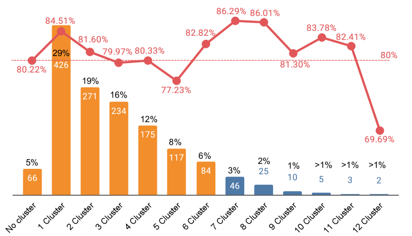
Figure 2: Our dataset consists of $1,464$ stimuli, we show the distribution of stimuli that got annotated with a certain number of clusters. User agreement is visualized in red for the number of clusters.

To illustrate our agreement score, Figure 3 shows two stimuli with corresponding annotations and different agreement scores, whereby both stimuli have been annotated by five participants. In the top row are $5$ annotations where participants showed strong agreement in the clustering, resulting in an average agreement score of $99.79\%$. In contrast, the bottom row shows annotations with an agreement score below $50\%$, where participants not only disagree on which points belong together, but one participant (most right) even indicated the absence of a cluster. Note that our score is independent of the order of clusters and, therefore also of cluster color. This means it only matters that points are drawn using the same color, but not with which color. In the top row of Figure 3, all $5$ users agreed on the number of clusters ($8$) and the corresponding shape of the clusters. In the bottom row, the users disagreed on any aspects, resulting in a relatively low agreement score. Additionally, in Figure 2 it becomes apparent, that for an increasing number of clusters the occurrence of data samples decreases. Looking at cluster numbers greater than $6$ clusters, the amount of data samples is below $5\%$, an insignificant number of samples to make general assumptions. Therefore, we exclude such stimuli from our training set, and included only those which are highlighted in Figure 2.

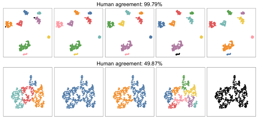
Figure 3: Comparison of two scatterplots used in our study. The top row shows a strong average agreement score of $99.79\%$, while the bottom row has a low average agreement score below $50\%$.

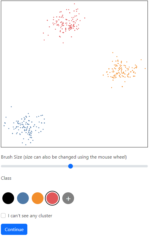
Figure 4: Web interface used for the crowdsource study in order to collect point-wise annotations from human observers. The shown scatterplot is a sanity check to filter out click-through participants.

4 ClusterNet

To be able to learn and imitate human cluster perception based on our large-scale point-based clustering dataset, we propose ClusterNet, a model that learns to cluster point-based data from human annotations. In this section, we will first discuss ClusterNet’s architecture (see Subsection 4.1), before discussing the loss we used for training ClusterNet (see Subsection 4.2).

4.1 Model Architecture

While ClusterNet shall be used as an alternative to exiting clustering techniques, it shall not learn on image data, as this requires rendering in a pre-process step in order to apply ClusterNet. Therefore, such as existing clustering techniques, we directly operate on scattered data and output a point-wise prediction containing clustering results. Since the feature encoder of ClusterNet is based on PointNet++, it encodes point attributes like density and distances in the point features. ClusterNet has to be able to learn from our unstructured data, in which each point is associated with a cluster ID and points with the same cluster ID belong to the same cluster. Unfortunately, learning on such unstructured data poses several challenges. First, due to the unstructured and irregular nature of the scatterplot data, traditional convolutional neural network (CNN) architectures which expect a regular grid data structure are not applicable. This is an important aspect, since the ordering of our scattered point data, as stored on disk, might vary, without actually affecting the visualization. Such effects are sometimes overlooked in the visualization community, but have recently also been investigated for line graphs by other researchers [36]. For training ClusterNet, we need to take this aspect into consideration, such that its predictions become invariant over point ordering. Unfortunately, order-invariance is not only relevant with respect to the order of stored points, but also with respect to the order of clusters. When predicting clusters, we want ClusterNet to be invariant of the cluster IDs, since cluster IDs can be permutated, without affecting the correctness of the result. So we need to realize a model architecture and a loss, which are invariant to these orderings. Another challenge is the fact that our visual stimuli are often sparse, meaning they contain a large number of empty regions, it becomes more challenging to extract useful information from the data. Finally, since crowdsourcing annotations involves human raters, our training data set size is smaller than in other domains. Together with the noise naturally present in scatterplot data sets, this poses a high risk of overfitting.

To deal with the challenges outlined above, we have investigated techniques from the field of deep geometric learning, where order invariance is also an important aspect. In the past years, several point-based learning architectures have been proposed, which directly learn on point cloud data [37, 38, 39, 40, 41]. In order to build ClusterNet, we decided to adapt the well-known PointNet++[38] architecture to learn on our point-based scatterplot dataset, since it was demonstrated to perform well at semantic segmentation tasks. However, in their experiments they also apply their network to 2D point clouds, sampled from MNIST [42] images. We follow their example and fix the input size to $N=512$ points in Euclidean space and setting the z-axis of all points to $0$. The feature extractor consists of $4$ hierarchical layers, for both down sampling and up sampling stages, where we use point cloud sizes $256,128,64,8$ for farthest point sampling (FPS). Note, that we use a random initialized FPS during training, and fixing it for inference. Additionally, we change the implementation of PointNet++, that for each point, the encoder produces a vector of size $128$, before outputting a cluster probability $P$ and noise probability $P_{noise}$ for each point. The two outputs of our network have the shape $NxC$ and $Nx1$, where $C$ is the maximum number of clusters. However, commonly used loss functions like negative log likelihood would require a fixed cluster order, and are therefore not applicable, as it would mean that we relate the position of a cluster to the number of clusters present in the target. Having said this, during training the model would chase arbitrary gradients, resulting in the absence of convergence, which makes a specialized loss important.

4.2 Training Loss

In order to be not only invariant with respect to point order, but also with respect to cluster order, we borrow from the field of meta classification learning using a contrastive loss, as proposed by Hsu et al. [5, 43, 6]. Meta classification learning solves a multi-class problem by reformulating it as a binary-class problem. It optimizes a binary classifier for pairwise similarity prediction and through this process learns a multi-class classifier as a submodule. Therefore, we represent our cluster targets as a similarity matrix $\operatorname{\mathbb{S}}$, which encodes point-wise cluster affiliation. It has the form $\operatorname{\mathbb{S}}\in N^{2}$, where $N$ is the number of points in the scatterplot, and it is defined as:

$$\operatorname{\mathbb{S}}_{ij}=\begin{cases}1,&P_{i},P_{j}\text{same cluster (positive)}\\ 0,&\text{different cluster (negative)}\end{cases}$$ (1)

where $P_{i},P_{j}$ are points from the same scatterplot. This matrix contains positive samples for similar points, that belong to the same cluster, and negative samples for points that are dissimilar, not the same cluster. For clarification, we demonstrate the representation of our targets in Figure 5. It is clear, that permuting the order of points results in the same matrix with equal permutation applied.

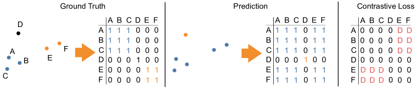
Figure 5: Scattered data with color coded clustering (left), and corresponding similarity matrix $\operatorname{\mathbb{S}}$, see Equation 1 (right).

Based on this cluster formulation, we can now define a measure to investigate agreement between targets, referring to it as agreement score $\operatorname{\hat{\operatorname{\alpha}}}$ and define it as follows:

$$\operatorname{\hat{\operatorname{\alpha}}}(R_{a},R_{b})=\frac{1}{N^{2}}\sum_{i}^{N}\sum_{j}^{N}{1-|\operatorname{\mathbb{S}}_{ij}(R_{a})-\operatorname{\mathbb{S}}_{ij}(R_{b})|}$$ (2)

where $R_{a},R_{b}$ are annotations of two users for the same scatterplot $R$. In order to compute agreement inside a group of $M$ targets, we can then compute an averaged agreement score for all possible combinations of two targets $\binom{M}{2}=K$ as follows:

$$\operatorname{\alpha}(G)=\frac{1}{K}\sum^{K}{\operatorname{\hat{\operatorname{\alpha}}}(R_{a},R_{b})}$$ (3)

Ultimately, representing targets in binary form using $\operatorname{\mathbb{S}}$ enables us to apply meta classification learning to our point-based ClusterNet, by minimizing the following loss term::

$$\mathfrak{L}_{mcl}=-\omega_{D}\sum_{ij}{\operatorname{\mathbb{S}}_{ij}\,log\,\hat{\operatorname{\mathbb{S}}}_{ij}\,+\,(1-\operatorname{\mathbb{S}}_{ij})\,log(1-\hat{\operatorname{\mathbb{S}}}_{ij})}$$ (4)

where $\omega_{D}$ is a weight matrix, that is used to rescale the momentum of negative samples in our contrastive loss. Further, we use it to correct the imbalanced error contribution of small clusters, accounting with fewer points to the loss function. We define such weight matrix as follows:

$$\omega_{D}(\operatorname{\mathbb{S}})=\begin{cases}\frac{1}{w_{c}^{2}},&\operatorname{\mathbb{S}}=1\\ D,&\operatorname{\mathbb{S}}=0\\ \end{cases}$$ (5)

where $D$ is the momentum of negative samples and $w_{c}$ is the cluster specific contribution $w_{c}=N_{c}/N$. $N_{c}$ is the number of points for a specific cluster $c$ and $N$ the total number of points.

Separating clusters in scattered data is not well-defined. While it might be obvious in some cases, in other cases points might not cluster at all. Also, outliers might be present in the scatterplot. In the following, we treat non-clustering points and outliers the same, calling it noise. In order to better capture the aspect of noise, we introduce another loss term $\mathfrak{L}_{noise}$. It is computed using a weighted binary cross entropy loss in order to counter strong class imbalances between positive (cluster) and negative (noise) samples. In our experiments we found, that scaling the weighting of negative samples by $9$ is beneficial, whereby we reserve cluster ID $0$ for points annotated as noise. In order to convert a multi-cluster target, that contains multiple cluster IDs, into a binary target, we replace all cluster IDs greater than $0$ with $1$. The loss term is then defined as follows:

$$\mathfrak{L}_{noise}=\frac{1}{N}\sum_{i}^{N}{0.9\,y_{i}\,log(p_{i})+0.1\,(1-y_{i})\,log(1-p_{i})}$$ (6)

Now, we can combine both loss terms into a weighted linear combination, whereby our loss term $L_{total}$ is composed using $\omega_{mcl}=0.1$ and $\omega_{noise}=1.0$ resulting in the following overall loss:

$$\mathfrak{L}_{total}=\mathfrak{L}_{mcl}\,\omega_{mcl}\,+\mathfrak{L}_{noise}\,\omega_{noise}$$ (7)

4.3 Training Protocol

To train ClusterNet, we use the Adam optimizer [44], with $betas=(0.9,0.999)$ and learning rate $1e-5$, reducing the learning rate by a factor of $10$ when the validation loss stagnates for $50$ epochs with batch size $32$. We divide our dataset in train ($1,171$ stimuli), validation ($87$) and test ($206$) split. During training, we apply random data augmentation to the input point clouds, using horizontal and vertical flips and random rotations between $-180$ and $180$ degrees, before normalizing all points clouds to be in range $-1.0$ and $1.0$ centered around the origin. Additionally, we adopt a random crop transformation, which performs random horizontal and vertical cuts through the points. Points from the left (top) side of the cutting line are moved to the right (bottom) side, and vise versa. We keep track of the clusters that get cut, in this way increasing the number of cluster annotations accordingly. For details on how we implement such data augmentation strategy, we refer the reader to our supplementary material.

5 Outlier-Aware Rater Agreement

In order to evaluate our model, we need to measure its performance on our test split. Many measures exist, that can quantify performance regarding different aspects. Therefore, selecting a metric, that is able to grasp the intended solution to our problem is crucial.

In order to evaluate ClusterNet, we need to be able to measure the ’agreement between an isolated rater and a group of raters’, which is computed by the Vanbelle Kappa Index [45] defined as:

$$\operatorname{\kappa_{v}}=\frac{\Pi_{T}-\Pi_{E}}{\Pi_{M}-\Pi_{E}}$$ (8)

with $\Pi_{T}$ being the theoretical agreement,$\Pi_{M}$ the maximum attainable agreement and $\Pi_{E}$ the agreement expected by chance. Thus, the Vanbelle Kappa Index computes values in the range of $-1$ (minimal agreement) and $1$ (perfect agreement). A value of $0$ relates to the agreement expected by chance. Note, Vanbelle and Albert indicate in their work, that if there is no variability in the rating of the isolated rater or by the group of raters, their index reduces to $\operatorname{\kappa_{v}}=1$ for perfect agreement, $\operatorname{\kappa_{v}}=0$ else, when $\Pi_{M}=\Pi_{E}$. Therefore, it is clear, that in the case of no cluster and single cluster, the variability tends to be zero, leading to $\operatorname{\kappa_{v}}=0$, if the group of raters does not perfectly agree. Although, these are rather rare cases.

Nevertheless, it is beneficial to employ a measure that is also sensible to outliers inside the group of raters, and that can even measure if an isolated rating can improve agreement inside the group. In order to do so, we use $\operatorname{\hat{\operatorname{\alpha}}}$ from Equation 2, and compute an averaged n-fold score $\operatorname{\alpha}$ for a given prediction $R$ and the group of users $G$. Therefore, we pick an annotation inside the group and replace it with $R$, yielding a modified group $G^{R}$. Then we compute $\operatorname{\alpha}(G^{R})$ and repeat this $N$ times, where $N$ is equal to the number of annotations in the group. Thus, we compute an agreement index $\operatorname{\kappa_{\operatorname{\alpha}}}$, that indicates if a given prediction improves agreement for $G$, when $\operatorname{\kappa_{\operatorname{\alpha}}}>0$ or decline when $\operatorname{\kappa_{\operatorname{\alpha}}}<0$. We define $\operatorname{\kappa_{\operatorname{\alpha}}}$ as follows:

$$\operatorname{\kappa_{\operatorname{\alpha}}}(R,G)=\frac{1}{N}\sum^{N}{\operatorname{\alpha}(G^{R}_{n})-\operatorname{\alpha}(G)}$$ (9)

where $G$ is the group of annotations and $G^{R}_{n}$ is the modified version of $G$ with the nth annotation replaced by $R$.

Since $\operatorname{\kappa_{v}}$ and $\operatorname{\kappa_{\operatorname{\alpha}}}$ do not capture outliers, we further adopt a noise index $\operatorname{\kappa_{n}}$, which computes the average of an n-fold binary Jaccard Index $\mathfrak{J}$ over the group of users and the prediction. This measure is defined as:

$$\operatorname{\kappa_{n}}(\hat{R},\hat{G})=\frac{1}{N}\sum^{N}{\mathfrak{J}(\hat{R},\hat{R}_{n})}$$ (10)

where $\hat{R}$ is the binary prediction for outliers. It encodes points associated with noise as $0$ and points affiliating with a cluster as $1$. $\hat{R_{n}}$ are the binary annotation of $G$ encoding noise.

Having defined these metrics, we will use them in the next section to evaluate ClusterNet’s results.

6 Experiments

In this section, we evaluate the results obtained from ClusterNet trained on our point-based scatterplot dataset. Similar to existing cluster algorithms like DBSCAN [1], Birch [2] and Optics [3], ClusterNet can predict on bi-variate data directly, rather than rendered scatterplot images. As described in Section 3, scatterplots used for crowdsourcing human annotations, originate from real bi-variate data, represented by arrays of 2D points. For evaluation of our experiments, we compute the three metrics proposed in Section 5 and report results averaged per group of cluster numbers. In order to compensate for imbalanced numbers of data samples per group, we compute the weighted average. Note, that $\operatorname{\kappa_{n}}$ is computed only for data samples that actually contain any noise labels.

6.1 Clustering Technique Comparison

ClusterNet is a model trained to predict human clustering for scattered data. In this experiment, we investigate the gap between existing clustering techniques and ClusterNet. Therefore, ten state-of-the-art clustering algorithms are compared using the implementation from scikit-learn. Since all approaches are parameterized, we first do a parameter search using our training dataset to find the specific optimized parameters for each technique. We then evaluate each approach using our test dataset and compare it against ClusterNet using the best model from Section 6.4. In LABEL:tab:clustering_technique_experiment, we report performance results for such clustering techniques. Note, that some techniques do not compute outliers, for which we do not calculate $\operatorname{\kappa_{n}}$. Looking at the results, we can see that ClusterNet outperforms all compared state-of-the-art approaches on all metrics. Looking at the $\operatorname{\alpha}$ measure, we can see, that predictions from ClusterNet almost perfectly agree with the group of users, indicated by a value close to zero. The Vanbelle Kappa Index $\operatorname{\kappa_{v}}$ also suggests a superior performance of ClusterNet over the other clustering techniques, which we interpret such that ClusterNet predictions agree with human annotators. Finally, examining the accuracy for noise or outlier prediction, ClusterNet has a slight advantage over DBSCAN, while both approaches clearly outperform Optics.

TABLE II: Comparison between ClusterNet and ten state-of-the-art clustering techniques using three test datasets: ours, SDR [21] and Data.gov . Some cluster techniques do not compute outliers, for which we omit evaluating $\operatorname{\kappa_{n}}$. Results highlighted with a * are from clustering techniques, that require priors about number of clusters, which is extracted from the ground truth annotation.

	ClusterNet	DBSCAN	OPTICS	Ward	Mean	Affinity	Spectral	Agglomerative	BIRCH	K-means	Gaussian Mixture
		[1]	[3]	[46]	Shift[47]	Propagation[48]	Clustering[49]	Clustering[50]	[2]	[51]	Model[52]
Evaluation on our test split
$\operatorname{\kappa_{\operatorname{\alpha}}}\uparrow$	-0.52	-4.13	-5.56	-1.04*	-6.90	-10.34	-2.65*	-7.02	-7.68	-1.49*	-0.90*
$\operatorname{\kappa_{v}}\uparrow$	0.69	0.62	0.56	0.66*	0.53	0.39	0.53*	0.38	0.38	0.63*	0.67*
$\operatorname{\kappa_{n}}\uparrow$	60.91%	55.49%	25.30%	-	-	-	-	-	-	-	-
Evaluation on SDR [21] data set.
$\operatorname{\kappa_{\operatorname{\alpha}}}\uparrow$	-1.49	-5.32	-4.25	-10.35*	-5.10	-11.43	-10.35*	-6.65	-7.11	-10.35*	-10.35*
$\operatorname{\kappa_{v}}\uparrow$	0.68	0.50	0.58	0.56*	0.61	0.36	0.56*	0.42	0.44	0.56*	0.56*
$\operatorname{\kappa_{n}}\uparrow$	58.07%	44.13%	31.56%	-	-	-	-	-	-	-	-
Evaluation on Data.gov
$\operatorname{\kappa_{\operatorname{\alpha}}}\uparrow$	0.03	-0.14	-1.94	-3.42*	-0.32	-2.04	-3.42*	-1.70	-0.94	-3.42*	-3.42*
$\operatorname{\kappa_{v}}\uparrow$	0.90	0.83	0.49	0.56*	0.79	0.46	0.56*	0.50	0.67	0.56*	0.56*
$\operatorname{\kappa_{n}}\uparrow$	53.66%	28.93%	17.68%	-	-	-	-	-	-	-	-
*The ground truth number of cluster was given to compute these scores.

6.2 Contrastive Loss Weighting Analysis

In Section 4.2, we proposed our contrastive loss function $\mathfrak{L}_{mcl}$, together with weight matrix $\omega_{D}$, which is used to rescale the momentum of negative samples. Depending on the scaling factor $D$, the weight matrix pushes apart dissimilar points. In this experiment, we demonstrate how this can be used to adjust the behavior of our model using different values for $D\in[0.1,1.0,10.0,50.0,100.0]$. To do so, we train five models using the protocol from above, and we report validation performance in LABEL:tab:weight_factor_experiment. Each model was trained for $37K$ steps and looking at the results, the model trained with weighting factor $D=50.0$ show slightly better results for $\operatorname{\alpha}$ and $\operatorname{\kappa_{v}}$, while noise prediction accuracy lacks behind the others. We see that, the model separates clusters stronger, for higher values of $D$ and merges clusters for small values. In the case for medium values of $D=10$ and $D=50$, the clustering results are more variable, increasing clustering performance, but also makes it harder for the model to differentiate between noise and cluster decision. However, in the following experiments, we can show that this effect reduces, for larger numbers of training steps, and we therefore use $D=50.0$ in the remaining experiments, if not stated otherwise.

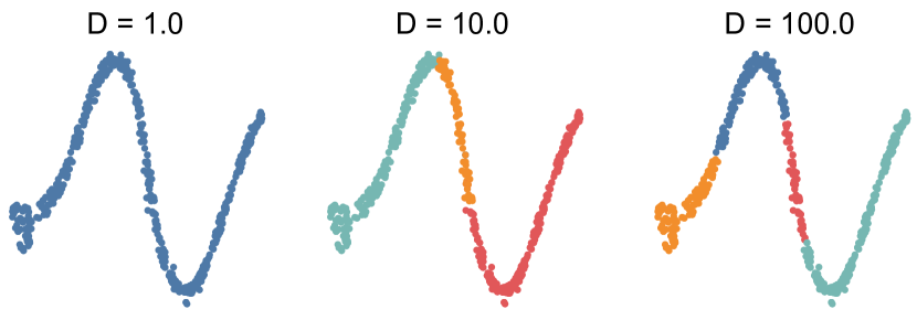
Figure 6: Predictions from three models, trained using different weighting factor $D=[1,10,100]$. Increasing the weighting produces predictions separating clusters more often.

TABLE III: Results of the contrastive loss weighting analysis (a), the human agreement analysis (b), and the fine-tuning analysis (c). We report performance results computing three metrics: $\operatorname{\kappa_{\operatorname{\alpha}}},\operatorname{\kappa_{v}},\operatorname{\kappa_{n}}$.

$D$	$\operatorname{\kappa_{\operatorname{\alpha}}}$	$\operatorname{\kappa_{v}}$	$\operatorname{\kappa_{n}}$
0.1	-5.64	0.53	49.97%
1.0	-6.33	0.43	48.09%
10.0	-2.01	0.61	46.26%
50.0	-1.66	0.62	45.91%
100.0	-1.78	0.61	50.76%

(a) Analysis of different weights $D$ for negative samples in our contrastive loss

$T_{agree}$	#samples	$\operatorname{\kappa_{\operatorname{\alpha}}}$	$\operatorname{\kappa_{v}}$	$\operatorname{\kappa_{n}}$
unfiltered	1171	-1.66	0.62	45.91%
50%	1148	-1.52	0.62	47.51%
60%	1049	-1.34	0.63	50.24%
70%	883	-0.55	0.68	58.48%
80%	672	-1.27	0.57	54.08%
90%	448	-1.66	0.58	53.92%

(b) Human agreement analysis by selecting different subsets of our data set

$D$	$T_{agree}$	$\operatorname{\kappa_{\operatorname{\alpha}}}$	$\operatorname{\kappa_{v}}$	$\operatorname{\kappa_{n}}$
0.01	$70\%$	-0.85%	0.66	57.07%
0.1	$70\%$	-0.52%	0.69	60.91%
1.0	$70\%$	-0.68%	0.67	52.36%

(c) Fine-tuning analysis of our best model by decreasing momentum for negative samples

6.3 Human Agreement Analysis

In Section 3.3 the agreement rate between users is discussed, and we showed that it is similar for different numbers of clusters. In this experiment, we investigate the impact of increasing human agreement during training for our model performance. To do so, we use a threshold $T_{agree}$ to filter our training dataset. We start by $T_{agree}=10\%$ and increase it in $10\%$ steps until we reach $T_{agree}=100\%$. For each threshold, we discard training samples, where the agreement score $\operatorname{\alpha}(G)<T_{agree}$. In Figure 7, we report the number of remaining training data for each threshold, as well as the resulting average agreement score. Looking at the different dataset sizes, we chose $5$ threshold values: $50\%,60\%,70\%,80\%,90\%$, to use in this experiment. We do not train a model using threshold $100\%$, since too few training samples would remain in order to expect a robust model. For threshold values below $50\%$, no training sample gets discarded, and we call this dataset unfiltered. In this experiment, we use a fixed negative momentum $D=50.0$.

The obtained results a shown in LABEL:tab:filter_agreement_experiment. The first row shows results from the model trained on all available training data, and is identical with the best model from the first experiment. The results suggest, that while increasing the level of agreement in the annotations, the test performance increases until reaching a maximum, see row number four. From this point on, filtering for higher agreement rates reduces the amount of training samples, while also decreasing model performance. We conclude from this experiment, that a certain degree of variance in the annotations, helps to improve model performance, and that our model achieves robustness through such variability. As a result, we use the model from row four in LABEL:tab:filter_agreement_experiment for our remaining experiments.

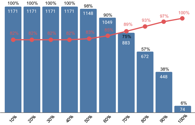
Figure 7: We filter the training dataset using different agreement thresholds $T_{agree}$, discarding training samples, where the agreement score is below such threshold. This results in different amounts of training data. For each threshold, we compute the resulting averaged agreement score for the remaining training data.

6.4 Fine-Tuning Analysis

After investigating the impact of weighting negative samples in Section 6.2 and maximizing user agreement in the training data in Section 6.3, we conduct a third experiment. Until now, we achieve the best results using a value of $D=50.0$ and an agreement threshold of $T_{agree}=70\%$. In our supplement material, we evaluate performance of such model for certain numbers of clusters, separately. We can show, that the largest error contribution originates from predictions for single clusters. This experiment investigates if, using smaller values of $D$, improves single cluster predictions. Therefore, we train three different models using momentum values $D=[0.01,0.1,1]$. In LABEL:tab:finetune_experiment, we report the performance results for all three models. Since the model has already learned to separate clusters, fine-tuning it to reduce its cluster separation ambitions must be done carefully. Therefore, we fine-tune each mode using a reduced learning rate of $10^{-7}$ for $8K$ training steps. Looking at the results, fine-tuning our model using a weighting factor $D=0.1$, helps to improve single cluster predictions and even overall performance of our model.

6.5 Generalization Analysis

In this experiment, we want to investigate the ability of ClusterNet to generalize to unseen data. Therefore, we use the dataset provided by the work of Sedmair [21], where 2D scatterplots are derived using dimensionality reduction techniques (SDR), consisting of real and synthetic data and apply identical crowdsource annotation procedure as described in Section 3. In such a way, we collect clusterings of $68$ participants for $272$ stimuli. Then, we evaluate the best model from Section 6.4 using this data set and report results for infering clusterings in LABEL:tab:clustering_technique_experiment and for regressing agreement predictions in Table IV. We can show, that ClusterNet outperforms existing clustering techniques in all three measures, $\operatorname{\kappa_{\operatorname{\alpha}}},\operatorname{\kappa_{v}},\operatorname{\kappa_{n}}$ indicating better alignments to human ratings and demonstrating the ability of ClusterNet generalizing to unseen data. In the upper eight rows of Figure 11 qualitative results are shown for ClusterNet generated during inference. These estimated clusterings for the SDR [21] test dataset underline well aligned predictions of ClusterNet to human judgments. In the next experiment, we investigate generalization to unbiased data by removing DR introducing potential projection bias to the data distribution.

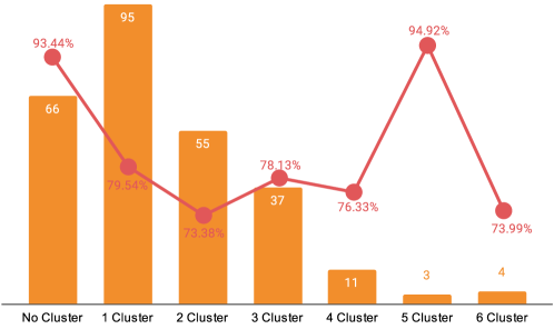
Figure 8: SDR [21] consists of $272$ stimuli, we show the distribution of stimuli that got annotated with a certain number of clusters. User agreement is visualized in red for the number of clusters.

6.6 Clustering in the Wild

Both data sets ClusterNet and SDR [21] apply dimensionality reduction (DR) techniques in order to derive 2D data for the application of different clustering approaches. In order to evaluate these approaches without a potential bias of the used DR technique, we collect a third data set without applying DR randomly sampling datasets from data.gov. The dimensionality of these datasets range from two to more than ten dimensions. Since we want to avoid the application of DR, we convert multi-dimensional data to bivarate data by randomly selecting two dimensions, as done by [24]. After visual inspection of the resulting scatterplots, we decide to crowdsource annotations from $20$ human raters per stimuli rather than only $5$ resulting in $50$ raters participating in the crowdsource study. We use the same web application described in Section 3.2 collecting human clusterings for $50$ stimuli. In Figure 9 the annotation and corresponding human rater agreement is displayed. Looking at the collected annotations, see Figure 9, human raters mainly perceived two clusters or less, while they agree more for the cases, when three or more clusters were selected. Finally, we use the best model from Section 6.4 and infer clustering and agreement predictions reporting results in LABEL:tab:clustering_technique_experiment and Table IV, respectively. Looking at the results, we can see that ClusterNet’s prediction slightly improve human rater agreement, indicated by a positive value of $\operatorname{\kappa_{\operatorname{\alpha}}}$. ClusterNet shows best scores for $\operatorname{\kappa_{v}}$ and $\operatorname{\kappa_{n}}$ amongst all competing clustering techniques, indicating well aligned clustering prediction to human judgment. In the bottom part of Figure 11, we present qualitative results of eight stimuli, taken from the Data.gov test dataset, showing superior performance of ClusterNet in comparison to existing clustering techniques.

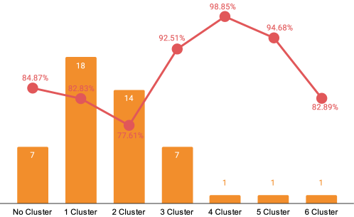
Figure 9: Data.gov consists of $50$ stimuli, we show the distribution of stimuli that got annotated with a certain number of clusters. User agreement is visualized in red for the number of clusters, respectively. Note, that for Data.gov per stimulus $20$ human raters provided clustering annotations.

6.7 Human Agreement Estimation

In Section 6.3, we investigated the effect of maximizing human agreement during training our model in order to learn a robust model. However, one question remains, what if human raters do not agree on a clustering. In Figure 10 on the left side, we display ratings of five human annotators for the same stimulus as well as the corresponding agreement rate amongst the group of raters, in the sixth column. In this experiment, we extend ClusterNet to output an agreement score $\operatorname{\alpha}$ in conjuction with cluster probability $P$ and noise probability $P_{noise}$ for each point. The estimation $\overline{\operatorname{\alpha}}$ of our network has the shape $Nx1$ and is computed by applying a Sidmoid activation to the network output. Training ClusterNet to predict $\operatorname{\alpha}$ is done by adding the agreement loss term to Equation 7, which is defined by:

$$\mathfrak{L}_{agree}=|\operatorname{\alpha}-\overline{\operatorname{\alpha}}|$$ (11)

where $\operatorname{\alpha}$ is the aggregated agreement score between all human raters, see Equation 3 and $\overline{\operatorname{\alpha}}$ is the prediction by ClusterNet. Note, that $\operatorname{\alpha}$ is computed per point without computing the average over all points. We use the identical finetune procedure as described in Section 6.4 and same hyperparameters and train ClusterNet on our collected training dataset and evaluate it on three test datasets: ClusterNet, SDR [21] and Data.gov and report results for five regression measures in Table IV. Looking at the results, it appears no large gap between all three datasets. There are slightly better test results for Data.gov indicated by the smallest $MaxErr$ value amongst all three, supporting the assumption of generalization to data out of distribution. In the last column of Figure 10, we display prediction results of ClusterNet for all three datasets, the first three rows for our test dataset, third to sixth row for SDR [21] and the last three rows for Data.gov stimulis. The first five rows display human annotations, note that we randomly sample five annotations for the last three rows, since for Data.gov we collected annotations from $20$ raters per stimulus.

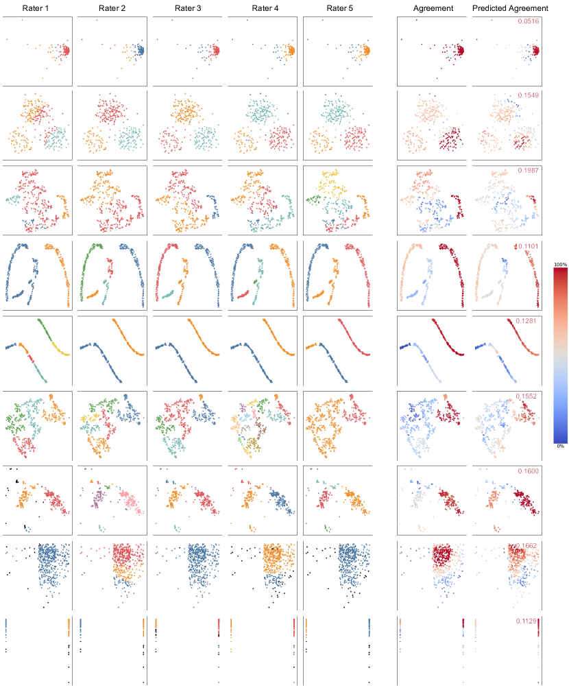
Figure 10: The first five column display human annotations collected during our online crowdsource study. We compare annotations for six stimuli. In the sixth column, the computed agreement score per point is shown. Finally, in the last column, the prediction of ClustetNet is shown, along with the averaged absolute error over all points.

Test dataset	MSE	$L_{1}$	$MSE_{log}$	MAE	MaxErr
ClusterNet	0.0305	0.1393	0.0101	0.1287	0.3068
SDR [21]	0.0317	0.1564	0.0100	0.1479	0.3029
Data.gov	0.0261	0.1451	0.0081	0.1362	0.2826

TABLE IV: We evaluate our model, that is trained on our dataset for the human agreement estimation task. We compute five regression metrics to measure it’s performance on three datasets: ClusterNet, the dataset SDR [21] , that consits of real and synthetic scatterplots and the dataset collected from Data.gov with real data without DR applied.

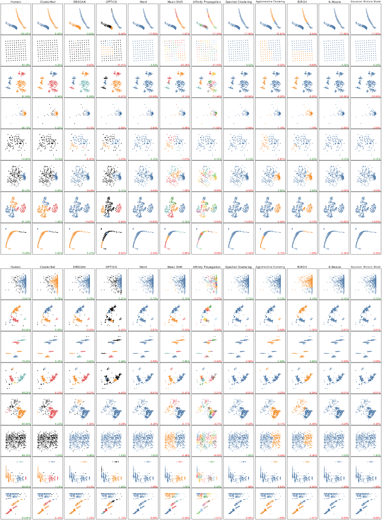
Figure 11: Qualitative evaluation results. The first eight rows are taken from the SDR [21] data set and the last eight rows from the Data.gov test dataset. Each column shows the results for a clustering technique. We compare our approach ClusterNet and ten existing clustering techniques, as well as the human rating with the maximum agreement inside the group of raters, in the first column. For each technique, the corresponding $\operatorname{\kappa_{\operatorname{\alpha}}}$ score is show in green, when the clustering improves group agreement and red, otherwise.

7 Limitations

While being the first of its kind, and performing well on human-like clustering, ClusterNet is not free of limitations. PointNet++ is order invariant with respect to the input point cloud, as is our contrastive loss term. However, the construction of the similarity matrix has a complexity of $O(n^{2})$. In our experiments, we used a fixed size for point clouds $N=512$, in order to keep computational costs low. As a result, we had to discard or randomly sample from real-world datasets, to match such requirements. However, in the field of contrastive learning, approaches like SimCLR [53] or SwAV [54] exist, which do not have this limitation and could be used to cluster points on the basis of their latent codes.

ClusterNet is trained on human annotated data collected during a crowdsourced study. Therefore, we rendered datasets using a fixed visual encoding, which limits the assumptions about agreement and perceived numbers of clusters to such visual encoding. So in cases, where visual encoding affects cluster perception, this would not be captured by ClusterNet. However, as argued above, we believe that as soon as visual encodings interfere with the clustering, the visual encoding should be reconsidered in the first place. Nevertheless, if wanted, our crowdsourced study could have also included variable visual encodings, and provide it as point features to our network during training. Thus, this is not strictly a limitation of ClusterNet, as more stimuli data could incorporate visual encodings during cluster prediction.

8 Discussion

ClusterNet is developed as an alternative to existing clustering techniques, that is specifically aligned to human perception. However, as discussed in Section 7, this work fixes the visual encoding during dataset construction in order to keep the desing space managable. Therefore, exploring the effect of visual design is subject to future research, while this work provides a promising baseline, that is able to generalize beyond unseen data. Further, our analysis of human agreement on clusterings show large varieties of the degree of agreement depending on the structure of the underlying data. It is questionable how meaningful a single clustering prediction is, for cases when a group of human raters provide ambiguous annotations. A generative model could be trained to produce many different such human aligned clusterings, reflecting the same human ambiguous distribution of annotation. In this work, we decided to predict an agreement score for each point, providing a neural feedback about the learned human discord. For a user of ClusterNet, this provides some understanding of the reliableness of the corresponding estimated clustering.

9 Conclusions and Future Work

We demonstrate ClusterNet, a clustering model based on human perceived clustering annotations. We collected a large-scale dataset using Prolific to crowdsource human point-wise clustering annotations. Investigation of the collected data, shows agreement above $80\%$ between human subjects. This dataset enables us to train ClusterNet, a learned clustering model, that mimics point clustering as performed by the human visual system. In multiple experiments, our protocol for training a point-based model is demonstrated, and we show how we fine-tune our model in order to adjust it to human annotations. In order to evaluate ClusterNet, we further proposed a novel metric, that measures agreement improvement, while also being sensible to annotation consistency. Ultimately, we evaluate our model using SDR [21] and Data.gov , which are datasets featuring unseen and out of scope data and compare it against ten state-of-the-art clustering techniques, whereby ClusterNet outperforms all compared algorithms demonstating it’s ability to generalize to new data. In our experiments, we also present how to deal with multiple correct clusterings, e.g. when multiple human judgments disagree on a particular stimulus. ClusterNet can be used to estimate human agreement, enabling to detect such ambiguities.

While we see ClusterNet as a milestone for perception-based clustering, we see several endeavors for future research. First, we could investigate the influence of the visual stimuli on cluster perception. Furthermore, we could facilitate the presented technology to learn other scatterplot tasks, such as for instance noise detection. Finally, we would like to investigate how ClusterNet can be used to optimize scatterplot visualization parameters.

Sebastian Hartwig is a Ph.D. student at Ulm University, Germany, where he previously received his B.Sc. and M.Sc. degrees in computer science. He completed his master’s degree at the Institute of Media Informatics in 2017 before joining the research group Visual Computing. His research focus on human perception based machine learning for computer graphics and visualization application, as well as machine scene understanding like depth and layout estimation.

Christian van Onzenoodt received his Master’s degree in Media Informatics from Ulm University in 2017.Following this, he was working as a research associate at the Visual Computing Group at Ulm University before he started working as a Data Engineer for the Liebherr International Group. His research interests are information visualization focusing on the perception of visualizations.

Pedro Hermosilla obtained his PhD in Computing at the Polytechnical University of Catalonia, under the supervision of Prof. Pere-Pau Vazquez and Prof. Alvar Vinacua. Later, he did a PostDoc at Ulm University with Prof. Timo Ropinski where he worked on developing machine learning technologies for 3D and unstructured data, with a particular interest in point clouds, graphs, and implicit representations. At the moment, he is an Assistant Professor in AI for Visual Computing at the Technical University of Wien, where he continues his research on these topics and how to apply such technologies to solve different problems in the fields of Computer Vision, Computer Graphics, and Bioinformatics.

Timo Ropinski is a professor at Ulm University, heading the Visual Computing Group. Before moving to Ulm, he was Professor in Interactive Visualization at Linköping University, heading the Scientific Visualization Group. He received his Ph.D. in computer science in 2004 from the University of Münster, where he also completed his Habilitation in 2009. Currently, Timo serves as chair of the EG VCBM Steering Committee, and as an editorial board member of IEEE TVCG.

References

- [1] M. Ester, H.-P. Kriegel, J. Sander, X. Xu et al., “A density-based algorithm for discovering clusters in large spatial databases with noise.” in kdd, vol. 96, no. 34, 1996, pp. 226–231.
- [2] T. Zhang, R. Ramakrishnan, and M. Livny, “Birch: A new data clustering algorithm and its applications,” Data mining and knowledge discovery, vol. 1, no. 2, pp. 141–182, 1997.
- [3] M. Ankerst, M. M. Breunig, H.-P. Kriegel, and J. Sander, “Optics: Ordering points to identify the clustering structure,” ACM Sigmod record, vol. 28, no. 2, pp. 49–60, 1999.
- [4] J. Xia, W. Lin, G. Jiang, Y. Wang, W. Chen, and T. Schreck, “Visual clustering factors in scatterplots,” IEEE Computer Graphics and Applications, vol. 41, no. 5, pp. 79–89, 2021.
- [5] Y.-C. Hsu and Z. Kira, “Neural network-based clustering using pairwise constraints,” arXiv preprint arXiv:1511.06321, 2015.
- [6] Y.-C. Hsu, Z. Lv, J. Schlosser, P. Odom, and Z. Kira, “Multi-class classification without multi-class labels,” arXiv preprint arXiv:1901.00544, 2019.
- [7] M. Aupetit, M. Sedlmair, M. M. Abbas, A. Baggag, and H. Bensmail, “Toward perception-based evaluation of clustering techniques for visual analytics,” in 2019 IEEE Visualization Conference (VIS). IEEE, 2019, pp. 141–145.
- [8] M. M. Abbas, M. Aupetit, M. Sedlmair, and H. Bensmail, “Clustme: A visual quality measure for ranking monochrome scatterplots based on cluster patterns,” in Computer Graphics Forum, vol. 38, no. 3. Wiley Online Library, 2019, pp. 225–236.
- [9] A. Sato and K. Yamada, “Generalized learning vector quantization,” Advances in neural information processing systems, vol. 8, 1995.
- [10] T. M. Martinetz, S. G. Berkovich, and K. J. Schulten, “’neural-gas’ network for vector quantization and its application to time-series prediction,” IEEE transactions on neural networks, vol. 4, no. 4, pp. 558–569, 1993.
- [11] K.-L. Du, “Clustering: A neural network approach,” Neural networks, vol. 23, no. 1, pp. 89–107, 2010.
- [12] J. Schnellbach and M. Kajo, “Clustering with deep neural networks–an overview of recent methods,” Network, vol. 39, 2020.
- [13] T. Kohonen, “Self-organizing maps: ophmization approaches,” in Artificial neural networks. Elsevier, 1991, pp. 981–990.
- [14] M. Ghaseminezhad and A. Karami, “A novel self-organizing map (som) neural network for discrete groups of data clustering,” Applied Soft Computing, vol. 11, no. 4, pp. 3771–3778, 2011.
- [15] R. Amarasiri, D. Alahakoon, and K. A. Smith, “Hdgsom: a modified growing self-organizing map for high dimensional data clustering,” in Fourth International Conference on Hybrid Intelligent Systems (HIS’04). IEEE, 2004, pp. 216–221.
- [16] J. Xia, L. Huang, W. Lin, X. Zhao, J. Wu, Y. Chen, Y. Zhao, and W. Chen, “Interactive visual cluster analysis by contrastive dimensionality reduction,” IEEE Transactions on Visualization and Computer Graphics, 2022.
- [17] C. Fan and H. Hauser, “Fast and accurate cnn-based brushing in scatterplots,” in Computer Graphics Forum, vol. 37, no. 3. Wiley Online Library, 2018, pp. 111–120.
- [18] ——, “On sketch-based selections from scatterplots using kde, compared to mahalanobis and cnn brushing,” IEEE Computer Graphics and Applications, vol. 41, no. 5, pp. 67–78, 2021.
- [19] G. J. Quadri and P. Rosen, “Modeling the influence of visual density on cluster perception in scatterplots using topology,” IEEE Transactions on Visualization and Computer Graphics, vol. 27, no. 2, pp. 1829–1839, 2020.
- [20] M. Abbas, E. Ullah, A. Baggag, H. Bensmail, M. Sedlmair, and M. Aupetit, “Clustrank: a visual quality measure trained on perceptual data for sorting scatterplots by cluster patterns,” arXiv preprint arXiv:2106.00599, 2021.
- [21] M. Sedlmair, T. Munzner, and M. Tory, “Empirical guidance on scatterplot and dimension reduction technique choices,” IEEE transactions on visualization and computer graphics, vol. 19, no. 12, pp. 2634–2643, 2013.
- [22] M. Sedlmair and M. Aupetit, “Data-driven evaluation of visual quality measures,” in Computer Graphics Forum, vol. 34, no. 3. Wiley Online Library, 2015, pp. 201–210.
- [23] M. Sips, B. Neubert, J. P. Lewis, and P. Hanrahan, “Selecting good views of high-dimensional data using class consistency,” in Computer Graphics Forum, vol. 28, no. 3. Wiley Online Library, 2009, pp. 831–838.
- [24] Y. Ma, A. K. Tung, W. Wang, X. Gao, Z. Pan, and W. Chen, “Scatternet: A deep subjective similarity model for visual analysis of scatterplots,” IEEE transactions on visualization and computer graphics, vol. 26, no. 3, pp. 1562–1576, 2018.
- [25] G. J. Quadri, J. A. Nieves, B. M. Wiernik, and P. Rosen, “Automatic scatterplot design optimization for clustering identification,” IEEE Transactions on Visualization and Computer Graphics, 2022.
- [26] A. V. Pandey, J. Krause, C. Felix, J. Boy, and E. Bertini, “Towards understanding human similarity perception in the analysis of large sets of scatter plots,” in Proceedings of the 2016 CHI Conference on Human Factors in Computing Systems, 2016, pp. 3659–3669.
- [27] A. Tatu, P. Bak, E. Bertini, D. Keim, and J. Schneidewind, “Visual quality metrics and human perception: an initial study on 2d projections of large multidimensional data,” in Proceedings of the international conference on advanced visual interfaces, 2010, pp. 49–56.
- [28] G. J. Quadri and P. Rosen, “A survey of perception-based visualization studies by task,” IEEE transactions on visualization and computer graphics, 2021.
- [29] V. Arel-Bundock, Rdatasets: A collection of datasets originally distributed in various R packages, 2023, r package version 1.0.0. [Online]. Available: https://vincentarelbundock.github.io/Rdatasets
- [30] L. Van der Maaten and G. Hinton, “Visualizing data using t-sne.” Journal of machine learning research, vol. 9, no. 11, 2008.
- [31] I. T. Jolliffe, Principal component analysis for special types of data. Springer, 2002.
- [32] S. Hartwig, M. Schelling, C. v. Onzenoodt, P.-P. Vázquez, P. Hermosilla, and T. Ropinski, “Learning human viewpoint preferences from sparsely annotated models,” in Computer Graphics Forum, vol. 41, no. 6. Wiley Online Library, 2022, pp. 453–466.
- [33] J. Heer and M. Bostock, “Crowdsourcing graphical perception: using mechanical turk to assess visualization design,” in Proceedings of the SIGCHI conference on human factors in computing systems. ACM, 2010, pp. 203–212.
- [34] M. Buhrmester, T. Kwang, and S. D. Gosling, “Amazon’s mechanical turk: A new source of inexpensive, yet high-quality, data?” Perspectives on psychological science, vol. 6, no. 1, pp. 3–5, 2011.
- [35] C. van Onzenoodt, P.-P. Vázquez, and T. Ropinski, “Out of the plane: Flower vs. star glyphs to support high-dimensional exploration in two-dimensional embeddings,” IEEE transactions on visualization and computer graphics, 2022.
- [36] T. Trautner and S. Bruckner, “Line weaver: Importance-driven order enhanced rendering of dense line charts,” in Computer Graphics Forum, vol. 40, no. 3. Wiley Online Library, 2021, pp. 399–410.
- [37] C. R. Qi, H. Su, K. Mo, and L. J. Guibas, “Pointnet: Deep learning on point sets for 3d classification and segmentation,” in Proceedings of the IEEE conference on computer vision and pattern recognition, 2017, pp. 652–660.
- [38] C. R. Qi, L. Yi, H. Su, and L. J. Guibas, “Pointnet++: Deep hierarchical feature learning on point sets in a metric space,” Advances in neural information processing systems, vol. 30, 2017.
- [39] P. Hermosilla, T. Ritschel, P.-P. Vázquez, À. Vinacua, and T. Ropinski, “Monte carlo convolution for learning on non-uniformly sampled point clouds,” ACM Transactions on Graphics (TOG), vol. 37, no. 6, pp. 1–12, 2018.
- [40] H. Jiang, F. Yan, J. Cai, J. Zheng, and J. Xiao, “End-to-end 3d point cloud instance segmentation without detection,” in Proceedings of the IEEE/CVF Conference on Computer Vision and Pattern Recognition, 2020, pp. 12 796–12 805.
- [41] Z. Ding, X. Han, and M. Niethammer, “Votenet: A deep learning label fusion method for multi-atlas segmentation,” in Medical Image Computing and Computer Assisted Intervention–MICCAI 2019: 22nd International Conference, Shenzhen, China, October 13–17, 2019, Proceedings, Part III 22. Springer, 2019, pp. 202–210.
- [42] Y. LeCun, L. Bottou, Y. Bengio, and P. Haffner, “Gradient-based learning applied to document recognition,” Proceedings of the IEEE, vol. 86, no. 11, pp. 2278–2324, 1998.
- [43] Y.-C. Hsu, Z. Lv, and Z. Kira, “Learning to cluster in order to transfer across domains and tasks,” arXiv preprint arXiv:1711.10125, 2017.
- [44] D. P. Kingma and J. Ba, “Adam: A method for stochastic optimization,” arXiv preprint arXiv:1412.6980, 2014.
- [45] S. Vanbelle and A. Albert, “Agreement between an isolated rater and a group of raters,” Statistica Neerlandica, vol. 63, no. 1, pp. 82–100, 2009.
- [46] F. Murtagh and P. Legendre, “Ward’s hierarchical clustering method: clustering criterion and agglomerative algorithm,” arXiv preprint arXiv:1111.6285, 2011.
- [47] D. Comaniciu and P. Meer, “Mean shift: A robust approach toward feature space analysis,” IEEE Transactions on pattern analysis and machine intelligence, vol. 24, no. 5, pp. 603–619, 2002.
- [48] B. J. Frey and D. Dueck, “Clustering by passing messages between data points,” science, vol. 315, no. 5814, pp. 972–976, 2007.
- [49] A. Ng, M. Jordan, and Y. Weiss, “On spectral clustering: Analysis and an algorithm,” Advances in neural information processing systems, vol. 14, 2001.
- [50] B. Moseley and J. Wang, “Approximation bounds for hierarchical clustering: Average linkage, bisecting k-means, and local search,” Advances in neural information processing systems, vol. 30, 2017.
- [51] J. A. Hartigan and M. A. Wong, “Algorithm as 136: A k-means clustering algorithm,” Journal of the royal statistical society. series c (applied statistics), vol. 28, no. 1, pp. 100–108, 1979.
- [52] H. Bensmail, G. Celeux, A. E. Raftery, and C. P. Robert, “Inference in model-based cluster analysis,” statistics and Computing, vol. 7, pp. 1–10, 1997.
- [53] T. Chen, S. Kornblith, M. Norouzi, and G. Hinton, “A simple framework for contrastive learning of visual representations,” in International conference on machine learning. PMLR, 2020, pp. 1597–1607.
- [54] M. Caron, I. Misra, J. Mairal, P. Goyal, P. Bojanowski, and A. Joulin, “Unsupervised learning of visual features by contrasting cluster assignments,” Advances in neural information processing systems, vol. 33, pp. 9912–9924, 2020.