Exploring the flavor structure of quarks and leptons with reinforcement learning

Abstract

We propose a method to explore the flavor structure of quarks and leptons with reinforcement learning. As a concrete model, we utilize a basic value-based algorithm for models with $U(1)$ flavor symmetry. By training neural networks on the $U(1)$ charges of quarks and leptons, the agent finds 21 models to be consistent with experimentally measured masses and mixing angles of quarks and leptons. In particular, an intrinsic value of normal ordering tends to be larger than that of inverted ordering, and the normal ordering is well fitted with the current experimental data in contrast to the inverted ordering. A specific value of effective mass for the neutrinoless double beta decay and a sizable leptonic CP violation induced by an angular component of flavon field are predicted by autonomous behavior of the agent. Our finding results indicate that the reinforcement learning can be a new method for understanding the flavor structure.

1 Introduction

The origin of flavor structure of quarks and leptons is one of the unsolved problems in particle physics. To understand the peculiar pattern of fermion masses and mixings, the flavor symmetries have been utilized to explain these flavor puzzle. An attractive feature of the flavor symmetry is that it may connect the bottom-up approach of flavor model building with the top-down approach based on an ultra-violet completion of the Standard Model such as the string theory. In this paper, we adopt a bottom-up approach to explore the flavor structure of quarks and leptons.

In most traditional approaches to address the flavor structure of quarks and leptons, one assumes a certain representation of quarks and leptons under the flavor symmetry among all possible configurations. Indeed, it will be difficult to exhaust all possible realistic flavor patterns from a broad theoretical landscape. For instance, in a global $U(1)$ flavor symmetric model using the Froggatt-Nielsen (FN) mechanism Froggatt:1978nt , we have a degree of freedom of $U(1)$ charge assignment of each quark and lepton. When we consider the flavor dependent $U(1)$ charges of the quarks $q_{i}$ within the range $-9\leq q_{i}\leq 9$, it results in ${\cal O}(10^{14})$ patterns of $U(1)$ charges even for the quark sector. When we combine with the lepton sector, we are faced with the problem of doing a brute-force search over a higher-dimensional parameter space. This is a simple flavor model using the continuous flavor symmetry, but in general, it is difficult to find a realistic flavor pattern from a huge amount of possibilities in flavor models with discrete symmetries. Thus, it motivates us to apply recent machine learning techniques for an exhaustive search of flavor models.

In order to explore such a huge landscape of flavor models, in this paper, we will deal with a reinforcement learning (RL), which is known as one of machine learning techniques . In the framework of RL, an agent autonomously discovers desirable behavior to solve given problems, where a systematic search is impossible. So far, such a technique was utilized to find the parameter space of FN models with an emphasis on the quark sector Harvey:2021oue , where only the experimental values of quark masses and mixing angles are efficiently reproduced. However, it is quite important to see whether one can reproduce the flavor structure of all the fermion masses and mixings. Throughout this paper, we assume the Type-I see-saw mechanism to realize active neutrino masses and large mixing angles in the lepton sector. We will utilize a basic value-based algorithm, where the neural network is trained by data given by an environment. To find the flavor structure of quarks and leptons efficiently, we set the environment where the inputs consist of $U(1)$ charges of quarks and leptons under the $U(1)$ flavor symmetry and the coefficients appearing in Yukawa couplings are randomly fixed as ${\cal O}(1)$ real values. The outputs of the neural network are probabilities for the action determined by a policy. Here, the action of agent is given by increasing or decreasing one of the $U(1)$ charges by one, and the agent receives the reward (punishment) for this action when the fermion masses and mixings determined by the $U(1)$ charges approach (deviate from) the experimental values. Specifically, the reward function is defined by the intrinsic value consisting of fermion masses and elements of CKM and PMNS matrices whose values are minimized under a vacuum expectation value (VEV) of complex flavon field.

In addition to reproducing the experimental values, parameter search with RL will provide new insights on the neutrino mass ordering and CP phase in the lepton sector. Note that a source of CP violation is assumed to be originating from the phase of complex flavon field. By training neural networks without specifying the neutrino mass orderings, RL can help to find whether the neutrinos are in the normal ordering or in the inverted ordering. From the results of trained network, we find that the normal ordering is statistically favored by the agent. Furthermore, the sizable Majorana CP phases and effective mass for the neutrinoless double beta decay are predicted around specific values.

This paper is organized as follows. After briefly reviewing RL with an emphasis on Deep Q-network in Sec. 2, we establish the FN model with RL in Sec. 3. We begin with the model building with RL by focusing on the quark sector in Sec. 4, and the training of the lepton sector is performed in Sec. 5. In particular, we analyze two scenarios for the neutrino sector. In Sec. 5.1, we implement the FN model with fixed neutrino mass ordering to the neural network, but the neutrino mass ordering is not specified in the analysis of Sec. 5.2. Sec. 6 is devoted to the conclusion and discussion. In Appendix B, we list our finding $U(1)$ charge assignment of quarks and leptons.

2 Reinforcement learning with deep Q-network

In this section, we briefly review RL with the Deep Q-Network (DQN) used in the analysis of this paper. For more details, see, e.g., Ref. RL . The RL is constructed by an agent and an environment. At a certain time, the agent observes the environment and takes some action. Depending on the change of the environment caused by the action, the agent will receive rewards or penalties. By repeating those processes and searching for actions that maximize the total rewards, the agent is designed to exhibit autonomous behavior in the environment.

To determine the action, we utilize the neural network model. In the multi-layer perceptrons, a $n$-th layer with $N_{n-1}$-dimensional vector $\vec{x}_{n-1}=(x_{n-1,1},x_{n-1,2},\cdots,x_{n-1,N_{n-1}})$ in multi-layer perceptrons transforms into a $N_{n}$-dimensional vector $\vec{x}_{n}=(x_{n,1},x_{n,2},\cdots,x_{n,N_{n}})$:

$$x_{n,i}=h_{n}(w_{ij}^{n}x_{n-1,j}+b_{i}^{n}),$$ (2.1)

with $h,w,b$ being the activation function, the weight and the bias, respectively. In the analysis of this paper, we employ a fully-connected layer. Then, the DQN known as one of the RL methods is characterized by Q network, target network, and experience replay. In this paper, we consider the neural networks whose output can be constructed by a softmax layer. Note that Q network and target network have same structures, but weights and biases in those are generically different from each other.

RL using the DQN proceeds through the following 5 steps:

1. An agent observes the environment state $s$ which is given as an input in the target neural network, as shown in Fig. 1. The target network (TN) gives the probabilities $p$ as an output. Since we adopt the softmax layer defined by

   $$f:\mathbb{R}^{n}\rightarrow[0,1]^{n},$$ (2.2)

   with $f({\bf x})_{i}=e^{x_{i}}/\sum_{i=1}^{n}e^{x_{i}}$, the output will also be regarded as probabilities.

   

   Figure 1: As a first step, the state $s$ observed by the agent is given as input in the target network.

2. In a second step, the agent determine the action $\mathfrak{a}$, taking into account the probabilities $p$ given by the first step. At the initial stage, the neural network cannot judge whether the action is an appropriate one. Let us denote the action with the highest probability $\mathfrak{b}$. To acquire the ability of autonomous behavior for the agent, we adopt the $\epsilon$-greedy method, where the greedy action $\mathfrak{b}$ is selected with probability $1-\epsilon$ and a random action $\mathfrak{c}$ is selected with probability $\epsilon$ (see Fig. 2), that is,

   $$\mathfrak{a}=\left\{\begin{array}[]{l}\mathfrak{b}\quad(\text{with}\,1-\epsilon)\\ \mathfrak{c}\quad(\text{with}\,\epsilon)\end{array}\right..$$ (2.5)

   

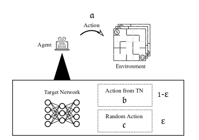
   Figure 2: In the second step, the agent selects the action $\mathfrak{a}$ through the $\epsilon$-greedy policy.

   By repeating this process, a sequence of the states is defined as follows:

   $$s_{1}\xrightarrow{\mathfrak{a}_{1}}s_{2}\xrightarrow{\mathfrak{a}_{2}}s_{3}\xrightarrow{\mathfrak{a}_{3}}\cdots,$$ (2.6)

   and this chain is called an episode. The initial environment state $s_{1}$ is chosen randomly. The number of actions is specified by $N_{\rm step}$ for one episode and the agent repeats this step $N_{\rm ep}$ times as shown in Table 1. Note that the greedy action is determined by taking into account the probabilities $p$ in the first step. The value of $\epsilon$ is chosen to ensure that the agent gradually takes the greedy action, whose explicit form will be given by

   $$\epsilon=\max\left(\epsilon_{0}r^{k-1},\ \epsilon_{\rm min}\right),$$ (2.7)

   with $k=1,2,...,N_{\rm ep}$. In the following analysis, we adopt $\epsilon_{0}=1,\ r=0.99999$ and $\epsilon_{\rm min}=0.01$. This definition means that the agent gains various experiences for the large $\epsilon$, using which the agent gradually takes a plausible action.

   	Step 1	Step 2	$\cdots$	Step $N_{\rm step}$
   Episode 1	$s_{1}^{1}$	$s_{2}^{1}$	$\cdots$	$s_{N_{\rm step}}^{1}$
   Episode 2	$s_{1}^{2}$	$s_{2}^{2}$	$\cdots$	$s_{N_{\rm step}}^{2}$
   $\vdots$	$\vdots$	$\vdots$	$\cdots$	$\vdots$
   Episode $N_{\rm ep}$	$s_{1}^{N_{\rm ep}}$	$s_{2}^{N_{\rm ep}}$	$\cdots$	$s_{N_{\rm step}}^{N_{\rm ep}}$

   Table 1: The environment states $s$ are changed by the actions. The agent performs at most $N_{\rm step}$ step for one episode.

3. The state $s$ is updated to $s^{\prime}$ through the action $\mathfrak{a}$. Depending on the states $s^{\prime}$, the agent receives a reward ${\cal R}$. In a third step, the transition $e=\langle s,\mathfrak{a},s^{\prime},{\cal R}\rangle$ corresponding to trajectories of experience is stored in the replay buffer as seen in Fig. 3.

   

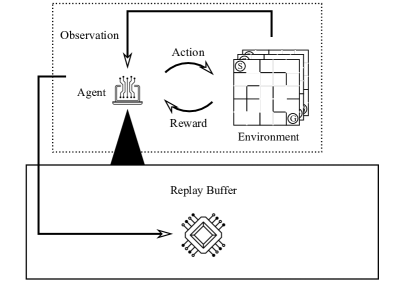
   Figure 3: In the third step, the transition $e=\langle s,\mathfrak{a},s^{\prime},{\cal R}\rangle$ is stored in the replay buffer.

4. A fourth step consists of “experience replay” and “stochastic gradient method”. The experience replay is to extract a mini-batch of transitions randomly sampled from the replay buffer, where the Q network is optimized by using at most a batch of transitions times epoch number. The advantage of this experience replay is twofold. First, the transitions in a batch are uncorrelated due to the random selection of past experiences. Second, one can reuse each transition in the training because all the experience is stored in the replay buffer.

   In the framework of DQN, there are two neural networks: Q network and target network. The Q network is updated by the stochastic gradient method where the mini-batch of transitions is used in the training data (see Fig. 4). When we denote outputs of the Q network and the target network by $y(s)$ and $y^{\prime}(s^{\prime})$, respectively, the weights and the biases are updated by minimizing a loss function $L(y,y^{\prime})$. In this paper, we adopt the Huber function:

   $$\begin{split}L_{\rm Huber}(y,y^{\prime})=\left\{\begin{array}[]{l}\frac{1}{2}(y^{\prime}_{\left({\cal R}\right)i}-y_{i})^{2}\qquad\qquad\,\,\,\,\text{if}\ |y^{\prime}_{\left({\cal R}\right)i}-y_{i}|\leq\delta\\ \delta\cdot|y^{\prime}_{\left({\cal R}\right)i}-y_{i}|-\frac{1}{2}\delta^{2}\qquad\text{if}\ |y^{\prime}_{\left({\cal R}\right)i}-y_{i}|>\delta\end{array}\right.,\end{split}$$ (2.8)

   with $y^{\prime}_{\left({\cal R}\right)}={\cal R}+\gamma y^{\prime},\ \gamma=0.99$ and $\delta=1$, which combines a mean squared error and a mean absolute error . Note that the training of Q network is carried out at the end of one episode, including at most the $N_{\rm step}$ step as shown in Table 1.

   

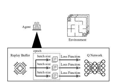
   Figure 4: In the fourth step, we randomly pick up the transitions with batch size from the replay buffer, and the weights and the biases of the Q network are updated by the stochastic gradient method in terms of these transitions.

5. The Q network and the target network have different parameters $\Theta=\{w,b\}$ and $\Theta^{\prime}=\{w^{\prime},b^{\prime}\}$, respectively. Lastly, the parameters $\Theta$ in the Q network are slightly reflected in $\Theta^{\prime}$ in the target network (see Fig. 5). Specifically, in the case of a soft update, this reflection proceeds as follows:

   $$\Theta^{\prime}\leftarrow(1-\alpha)\Theta^{\prime}+\alpha\Theta,$$ (2.9)

   where $\alpha$ is called the “learning rate”. This procedure can suppress rapid parameter changes and update the target network while maintaining learning stability. When $\alpha$ is large, the stability of the learning will be lost, but the small $\alpha$ will lead to a slow learning. In this paper, we adopt $\alpha=2.5\times 10^{-4}$. Since the stochastic gradient method is not used in updating the parameters of the target network as described above, no loss function is defined for this network.

   

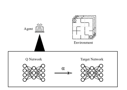
   Figure 5: In the last step, the weights and the biases of the target network are updated, following the soft update with the learning rate $\alpha$.

3 Froggatt-Nielsen model with reinforcement learning

3.1 The environment

In FN models, the hierarchical structure of fermion masses and the flavor structure are addressed by the global $U(1)$ symmetry. For simplicity, we introduce only one complex scalar field (so-called flavon field), charged under $U(1)$. The relevant Yukawa terms of quarks and leptons are given by

$${\cal L} =y^{u}_{ij}\left(\frac{\phi}{M}\right)^{n^{u}_{ij}}\bar{Q}_{i}H^{c}u_{j}+y^{d}_{ij}\left(\frac{\phi}{M}\right)^{n^{d}_{ij}}\bar{Q}_{i}Hd_{j}+y^{l}_{ij}\left(\frac{\phi}{M}\right)^{n^{l}_{ij}}\bar{L}_{i}Hl_{j}$$

$$+y^{\nu}_{ij}\left(\frac{\phi}{M}\right)^{n^{\nu}_{ij}}\bar{L}_{i}H^{c}N_{j}+\frac{y^{N}_{ij}}{2}\left(\frac{\phi}{M}\right)^{n^{N}_{ij}}M\bar{N}^{c}_{i}N_{j}+\text{h.c.},$$ (3.1)

where $\{Q_{i},u_{i},d_{i},L_{i},l_{i},N_{i},H\}$ denote the left-handed quarks, the right-handed up-type quarks, the right-handed down-type quarks, the left-handed leptons, the right-handed charged leptons, the right-handed neutrinos, and the SM Higgs doublet with $H^{c}=i\sigma_{2}H^{\ast}$, respectively. Here, we assume three right-handed neutrinos and tiny neutrino masses are generated by Type-I seesaw mechanism where the parameter $M$ is chosen as $M=10^{15}$ GeV throughout the analysis of this paper, and the Yukawa couplings $\{y^{u}_{ij},y^{d}_{ij},y^{l}_{ij},y^{\nu}_{ij},y^{N}_{ij}\}$ are ${\cal O}(1)$ real coefficients. Since the SM fields and the flavon field are also charged under $U(1)$, let us denote their $U(1)$ charges by

$$\{q(Q_{i}),\,q(u_{i}),\,q(d_{i}),\,q(L_{i}),\,q(l_{i}),\,q(N_{i}),\,q(H),\,q(\phi)\}.$$ (3.2)

To be invariant under the $U(1)$ symmetry, the integers $n_{ij}$ satisfy the following relations:

$$\begin{split}n^{u}_{ij}&=-\frac{q(\bar{Q}_{i}H^{c}u_{j})}{q(\phi)}=-\frac{-q(Q_{i})-q(H)+q(u_{j})}{q(\phi)},\\ n^{d}_{ij}&=-\frac{q(\bar{Q}_{i}Hd_{j})}{q(\phi)}=-\frac{-q(Q_{i})+q(H)+q(d_{j})}{q(\phi)},\end{split}$$ (3.3)

$$\begin{split}n^{l}_{ij}&=-\frac{q(\bar{L}_{i}Hl_{j})}{q(\phi)}=-\frac{-q(L_{i})+q(H)+q(l_{j})}{q(\phi)},\\ n^{\nu}_{ij}&=-\frac{q(\bar{L}_{i}H^{c}N_{j})}{q(\phi)}=-\frac{-q(L_{i})-q(H)+q(N_{j})}{q(\phi)},\\ n^{N}_{ij}&=-\frac{q(\bar{N}_{i}^{c}N_{j})}{q(\phi)}=-\frac{q(N_{i})+q(N_{j})}{q(\phi)},\end{split}$$ (3.4)

where $n_{ij}$ are considered positive integers throughout this paper. Furthermore, we require the presence of Yukawa term $\bar{Q}_{3}H^{c}u_{3}$, irrelevant to $q(\phi)$:

$$q(\bar{Q}_{3}H^{c}u_{3})=0\leftrightarrow q(H)=q(u_{3})-q(Q_{3});$$ (3.5)

otherwise one cannot realize the value of top quark mass. Once $\phi$ and $H$ develop VEVs, $\langle\phi\rangle=v_{\phi}$ and $\langle H\rangle=v_{\rm EW}=174\,$GeV, the Dirac mass matrices of quarks and leptons as well as the Majorana mass matrix are given by

$$\begin{split}m_{ij}^{u}&=y^{u}_{ij}\epsilon^{n^{u}_{ij}}v_{\rm EW},\qquad m_{ij}^{d}=y^{d}_{ij}\epsilon^{n^{d}_{ij}}v_{\rm EW},\qquad\\ m_{ij}^{l}&=y^{l}_{ij}\epsilon^{n^{l}_{ij}}v_{\rm EW},\qquad m_{Dij}^{\nu}=y^{\nu}_{ij}\epsilon^{n^{\nu}_{ij}}v_{\rm EW},\qquad m_{ij}^{N}=My^{N}_{ij}\epsilon^{n^{N}_{ij}}.\end{split}$$ (3.6)

The light neutrino mass matrix is obtained by integrating out heavy right-handed neutrinos:

$$m_{ij}^{\nu}=-\left(m^{\nu}\cdot(m^{N})^{-1}\cdot(m^{\nu})^{T}\right)_{ij}.$$ (3.7)

The quark and lepton mass matrices are diagonalized as

$$\begin{split}m^{u}&=U^{u}{\rm diag}(m^{u})(V^{u})^{\dagger},\qquad m^{d}=U^{d}{\rm diag}(m^{d})(V^{d})^{\dagger},\qquad\\ m^{l}&=U^{l}{\rm diag}(m^{l})(V^{l})^{\dagger},\qquad m^{\nu}=U^{\nu}{\rm diag}(m^{\nu})(U^{\nu})^{T},\end{split}$$ (3.8)

and the flavor mixings are given by the difference between mass eigenstates and flavor eigenstates:

$$\begin{split}V_{\rm PMNS}&=(U^{l})^{\dagger}V^{\nu}\\ &=\begin{pmatrix}c_{12}c_{13}&s_{12}c_{13}&s_{13}e^{-i\delta_{\rm CP}}\\ -s_{12}c_{23}-c_{12}s_{23}s_{13}e^{i\delta_{\text{CP}}}&c_{12}c_{23}-s_{12}s_{23}s_{13}e^{i\delta_{\text{CP}}}&s_{23}c_{13}\\ s_{12}s_{23}-c_{12}c_{23}s_{13}e^{i\delta_{\text{CP}}}&-c_{12}s_{23}-s_{12}c_{23}s_{13}e^{i\delta_{\text{CP}}}&c_{23}c_{13}\end{pmatrix}\begin{pmatrix}1&0&0\\ 0&e^{i\frac{\alpha_{21}}{2}}&0\\ 0&0&e^{i\frac{\alpha_{31}}{2}}\end{pmatrix},\end{split}$$ (3.9)

with $c_{ij}=\cos\theta_{ij}$ and $s_{ij}=\sin\theta_{ij}$, which also holds for the CKM matrix $V_{\rm CKM}=(U^{u})^{\dagger}U^{d}$ in the quark sector except the Majorana phases $\{\alpha_{21},\alpha_{31}\}$. Since the quarks and the leptons are charged under $U(1)$, the flavon VEV $\langle\phi\rangle=v_{\phi}$ will lead to the flavor structure due to the smallness of $|\epsilon|$:

$$\epsilon:=\frac{v_{\phi}}{M}.$$ (3.10)

Recalling that the $U(1)$ charge of Higgs doublet is determined by Eq. (3.5), the flavor structure of quarks and leptons is specified by the following charge vector:

$${\cal Q}_{a}:=\{q(Q_{i}),\,q(u_{i}),\,q(d_{i}),\,q(L_{i}),\,q(l_{i}),\,q(N_{i}),\,q(\phi)\},$$ (3.11)

consisting of 19 elements. This is the input for target network and Q network as the state $s$. In the following analysis using RL, we restrict ourselves to the following range of $U(1)$ charge:

$$-9\leq{\cal Q}_{a}\leq 9,$$ (3.12)

corresponding to total $19^{19}\sim 10^{24}$ possibilities for the charge assignment. It will be a challenging issue to find a realistic flavor pattern by the brute force approach. Furthermore, it is generally difficult to use the gradient descent method, because the $U(1)$ charges are discrete and even a small difference in the charges will result in exponential differences in calculated values such as masses. Against those backgrounds, the necessity of applying reinforcement learning arises. Note that a generic $U(1)$ charge of flavon will lead to the non-integer $n_{ij}$; thereby we focus on $q(\phi)=1$ or $-1$ with 50% probability in the following analysis.

3.2 Neural Network

A state $s$ given by the charge assignment ${\cal Q}$ will be updated to $s^{\prime}$ through the action $\mathfrak{a}$. To determine the action, we utilize the neural network as shown in Table 2. The activation function $h$ (in Eq.(2.1)) is chosen as a SELU function for hidden layers 1,2,3 and the softmax function (2.2) for the output layer. We employ the ADAM optimizer in TensorFlow DBLP:journals/corr/AbadiABBCCCDDDG16 , where the weights and biases are chosen to minimize the loss function given by the Huber function (2.8).

In the FN model, the flavor structure of quarks and leptons is determined by the charge vector ${\cal Q}_{a}$, including total $10^{24}$ possibilities for the charge assignment as pointed out before. When we focus on only the quark sector, the parameter spaces of $U(1)$ charges reduce to $19^{10}\sim 10^{12}$ possibilities. To achieve a highly efficient learning in a short time, it is better to perform a separate training for the $U(1)$ charge assignment of quarks and leptons. Note that only the flavon $U(1)$ charge connects the quark sector with the lepton sector since the $U(1)$ charge of the Higgs is determined by the charge of third generation quarks (3.5). As mentioned before, we focus on $q(\phi)=1$ or $-1$ with 50% probability in the following analysis. Thus, we first analyze the parameter space of quark $U(1)$ charges by RL as will be discussed in detail in Sec. 4, and move to the lepton sector with fixed $U(1)$ charge of Higgs fields as will be discussed in detail in Sec. 5.

The hyperparameters are set as $N_{\rm ep}=10^{5}$ and $N_{\rm ep}=6\times 10^{4}$ for the episode number in the quark and lepton sector respectively, $N_{\rm step}=32$ for the step number, batch sizes of 32, epoch number of 32, and the learning rate $\alpha=2.5\times 10^{-4}$, respectively. The hyperparameters in $\epsilon$-greedy method are described in the previous section. About the step number $N_{\rm step}=32$, the same value was used in the previous research that focuses on only the quark sector Harvey:2021oue . In Ref. Harvey:2021oue , it was shown that terminal states can be reached after a sufficient amount of learning. Therefore, it is expected that $N_{\rm step}=32$ is enough to achieve terminal states in the current situation where the quark sector and the lepton sector are searched separately.

layer	Input	Hidden 1	Hidden 2	Hidden 3	Output
Dimension	$\mathbb{Z}^{A}$	$\mathbb{R}^{64}$	$\mathbb{R}^{64}$	$\mathbb{R}^{64}$	$\mathbb{R}^{2A}$

Table 2: In the neural network, the input is the charge assignment ${\cal Q}_{a}$ with dimension $A$, and the activation functions are the SELU function for hidden layers 1,2,3. Since we use the softmax function (2.2) for the output layer, the output with dimension $2A$ is interpreted as probabilities. The dimension of the output layer is twice that of the input layer due to the action of the agent (3.13).

3.3 Agent

To implement the FN model in the context of RL with DQN, we specify the following action $\mathfrak{a}$ of the agent at each step:

$$\mathfrak{a}\,:\,{\cal Q}_{a}\rightarrow{\cal Q}_{a}\pm 1\,\,(a\in A),$$ (3.13)

where $A$ corresponds to $\{Q_{i},u_{i},d_{i},\phi\}$ in the analysis of Sec. 4 and $\{L_{i},l_{i},N_{i},\phi\}$ in the analysis of Sec. 5. These two candidates of the action make the dimension of the output layer $2A$ in Table 2. At the initial stage, the ${\cal O}(1)$ coefficients in Yukawa terms (3.1) are picked up from the two Gaussian distribution with an average $\pm 1$ and standard deviation 0.25 (see Fig. 6) and after the training by neural network introduced in the previous section, they are optimized to proper values by the Monte-Carlo simulation.

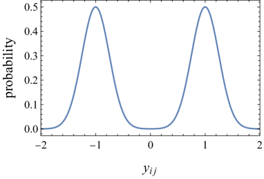
Figure 6: Distribution of ${\cal O}(1)$ coefficients in Yukawa terms (3.1).

Thus, once the charges are fixed, one can compare the masses and mixings of quarks or leptons given by the action $\mathfrak{a}$ with the experimental values. Specifically, we define the intrinsic value:

$$\begin{split}{\cal V}({\cal Q})=\left\{\begin{array}[]{ll}-{\rm min}_{v_{\phi}}\bigl{[}{\cal M}_{\rm quark}+{\cal C}\bigl{]}&\quad({\rm used\,in\,Sec.\,\ref{sec:quark}})\\ -\bigl{[}{\cal M}_{\rm lepton}+{\cal M}_{\rm neutrino}+{\cal P}\bigl{]}&\quad({\rm used\,in\,Sec.\,\ref{sec:lepton}})\end{array}\right.\end{split},$$ (3.14)

whose components will be defined below. Note that the flavon VEV is chosen to maximize the intrinsic value relevant for the quark sector in Sec. 4; thereby there is no flavon dependence in the intrinsic value of the lepton sector.

1. Quark and lepton masses:

   ${\cal M}_{\rm quark}$ (${\cal M}_{\rm lepton}$) consists of the ratio of the predicted quark (lepton) masses by the agent to the experimental values:

   $${\cal M}_{\rm quark}=\sum_{\alpha=u,d}E_{\alpha},\qquad{\cal M}_{\rm lepton}=\sum_{\alpha=l}E_{\alpha},$$ (3.15)

   with

   $$E_{\alpha}=\biggl{|}\log_{10}\left(\frac{|m_{\alpha}|}{|m_{\alpha,{\rm exp}}|}\right)\biggl{|}.$$ (3.16)

   The experimental values are listed in Tables 3 and 4 for quarks and leptons, respectively.

2. Neutrino masses:

   Since the ordering of neutrino masses has not been confirmed yet, we search the neutrino structure in two cases: RL with fixed neutrino mass ordering in Sec. 5.1 and RL without specifying the neutrino mass ordering in Sec. 5.2. In each case, the intrinsic value relevant to the neutrino masses is defined as:

   $${\cal M}_{\rm neutrino}=\left\{\begin{array}[]{ll}\sum_{\alpha=\nu_{21},\nu_{31}}E_{\alpha}^{\nu}&\quad({\rm normal\,ordering\,in\,Sec.\,\ref{sec:neutrino1}})\\ \sum_{\alpha=\nu_{21},\nu_{32}}E_{\alpha}^{\nu}&\quad({\rm inverted\,ordering\,in\,Sec.\,\ref{sec:neutrino1}})\\ 0&\quad({\rm unspecified\,mass\,ordering\,in\,Sec.\,\ref{sec:neutrino2}})\end{array}\right.,$$ (3.20)

   with

   $$E_{\alpha}^{\nu}=\biggl{|}\log_{10}\left(\frac{|\Delta m_{\alpha}^{2}|}{|\Delta m^{2}_{\alpha,{\rm exp}}|}\right)\biggl{|},$$ (3.21)

   where the experimental values are listed in Table 4.

3. Mixing angles:

   In addition, the intrinsic value includes the information of quark mixings and lepton mixings in ${\cal C}$ and ${\cal P}$:

   $${\cal C}=\sum_{i,j}E_{\cal C}^{ij},\qquad{\cal P}=\sum_{i,j}E_{\cal P}^{ij},$$ (3.22)

   with

   $$E_{\cal C}^{ij}=\biggl{|}\log_{10}\left(\frac{|V_{\rm CKM}^{ij}|}{|V_{\rm CKM,\,exp}^{ij}|}\right)\biggl{|},\quad E_{\cal P}^{ij}=\biggl{|}\log_{10}\left(\frac{|V_{\rm PMNS}^{ij}|}{|V_{\rm PMNS,\,exp}^{ij}|}\right)\biggl{|},$$ (3.23)

   where $E_{\cal C}^{ij}$ and $E_{\cal P}^{ij}$ represent the ratio of the predicted quark and lepton mixings by the agent to the experimental values, respectively. From Tables 3 and 4, the CKM and PMNS matrices are of the form:

   $$\begin{split}|V_{\rm CKM,\,exp}|&=\left(\begin{array}[]{lll}0.97435\pm 0.00016&\,\,0.22500\pm 0.00067&\,\,0.00369\pm 0.00011\\ 0.22486\pm 0.00067&\,\,0.97349\pm 0.00016&\,\,0.04182_{-0.00074}^{+0.00085}\\ 0.00857_{-0.00018}^{+0.00020}&\,\,0.0410_{-0.00072}^{+0.00083}&\,\,0.999118_{-0.000036}^{+0.000031}\end{array}\right),\\ |V_{\rm PMNS,\,exp}|_{3\sigma}&=\left(\begin{array}[]{lll}0.803\rightarrow 0.845&\,\,0.514\rightarrow 0.578&\,\,0.143\rightarrow 0.155\\ 0.244\rightarrow 0.498&\,\,0.502\rightarrow 0.693&\,\,0.632\rightarrow 0.768\\ 0.272\rightarrow 0.517&\,\,0.473\rightarrow 0.672&\,\,0.623\rightarrow 0.761\end{array}\right).\end{split}$$ (3.24)

$m_{u}$/MeV	$m_{d}$/MeV	$m_{s}$/MeV	$m_{c}$/GeV	$m_{b}$/GeV	$m_{t}$/GeV
$2.16^{+0.49}_{-0.26}$	${4.67}^{+0.48}_{-0.17}$	${93.4}^{+8.6}_{-3.4}$	${1.27}\pm{0.02}$	$4.18^{+0.03}_{-0.02}$	$172.69\pm 0.30$
$s_{12}$	$s_{13}$	$s_{23}$	$\delta_{\rm CP}$
$0.22500\pm 0.00067$	$0.00369\pm 0.00011$	$0.04182^{+0.00085}_{-0.00074}$	$1.144\pm 0.027$

Table 3: Masses, mixing angles, and CP phase in the quark sector ParticleDataGroup:2022pth , where we show the top-quark mass from direct measurements.

Observables	Normal Ordering (NO)		Inverted Ordering (IO)
	$1\sigma$ range	$3\sigma$ range	$1\sigma$ range	$3\sigma$ range
$\sin^{2}\theta_{12}$	$0.303_{-0.011}^{+0.012}$	$0.270\rightarrow 0.341$	$0.303_{-0.011}^{+0.012}$	$0.270\rightarrow 0.341$
$\sin^{2}\theta_{13}$	$0.02225_{-0.00059}^{+0.00056}$	$0.02052\rightarrow 0.02398$	$0.02223_{-0.00058}^{+0.00058}$	$0.02048\rightarrow 0.02416$
$\sin^{2}\theta_{23}$	$0.451_{-0.016}^{+0.019}$	$0.408\rightarrow 0.603$	$0.569_{-0.021}^{+0.016}$	$0.412\rightarrow 0.613$
$\delta_{\text{CP}}/\pi$	$1.29_{-0.14}^{+0.20}$	$0.80\rightarrow 1.94$	$1.53_{-0.16}^{+0.12}$	$1.08\rightarrow 1.91$
$\cfrac{\Delta m_{21}^{2}}{10^{-5}\mathrm{eV}^{2}}$	$7.41_{-0.20}^{+0.21}$	$6.82\rightarrow 8.03$	$7.42_{-0.20}^{+0.21}$	$6.82\rightarrow 8.04$
$\dfrac{\Delta m_{3l}^{2}}{10^{-3}\mathrm{eV}^{2}}$	$2.507_{-0.027}^{+0.026}$	$2.427\rightarrow 2.590$	$-2.486_{-0.028}^{+0.025}$	$-2.570\rightarrow-2.406$
$m_{e}$/MeV	$0.510999$
$m_{\mu}$/MeV	$105.658$
$m_{\tau}/\text{MeV}$	$1776.86$

Table 4: Experimental values for the lepton sector obtained from global analysis of the data, where $\Delta m_{3l}^{2}\equiv\Delta m_{31}^{2}=m^{2}_{3}-m^{2}_{1}>0$ for NO and $\Delta m_{3l}^{2}\equiv\Delta m_{32}^{2}=m^{2}_{3}-m^{2}_{2}<0$ for IO. Here, we use the data from Ref. ParticleDataGroup:2022pth for charged lepton masses and NuFIT v5.2 results with Super-Kamiokande atmospheric data for the lepton mixing angles and CP phase Esteban:2020cvm .

The flavon VEV is defined to maximize the intrinsic value, and we search for the VEV within

$$0.01\leq|v_{\phi}|\leq 0.3,\qquad-\pi\leq{\rm arg}(v_{\phi})\leq\pi,$$ (3.25)

where the angular component of the flavon VEV determines the CP phase. The large intrinsic value indicates that the obtained charge assignment well reproduces the experimental values. Such a charge assignment is called terminal state. Specifically, the terminal state is defined to satisfy the following requirement:

$$|{\cal V}({\cal Q})|<V_{0},\qquad E_{\alpha},E_{\alpha}^{\nu}<V_{1}\quad({\rm for}\,\forall\alpha),\qquad E_{{\cal C},{\cal P}}^{ij}<V_{2}\quad({\rm for}\,\forall i,j).$$ (3.26)

In this paper, we adopt $V_{0}=10.0$, $V_{1}=1.0$ and $V_{2}=0.2$. Here, $V_{1}=1.0$ ($V_{2}=0.2)$ means that the ratio of the predicted fermion masses (mixings) to the observed masses (mixings) is considered within $0.1\leq r_{\rm mass}\leq 10$ ($0.63\leq r_{\rm mixings}\leq 1.58$).

Let us denote the charge assignment ${\cal Q}$ observed by the agent and ${\cal Q}^{\prime}$ after the action $\mathfrak{a}$. For the action of the agent $({\cal Q},\mathfrak{a})$, we will give the reward $\mathcal{R}$ in the following prescription:

1. Give the basic point $\mathcal{R}_{\rm base}$, depending on the value of intrinsic value:

   $$\mathcal{R}_{\rm base}=\left\{\begin{array}[]{ll}{\cal V}({\cal Q}^{\prime})-{\cal V}({\cal Q})&\qquad{\rm if}\,{\cal V}({\cal Q}^{\prime})-{\cal V}({\cal Q})>0\\ \mathcal{R}_{\rm offset}&\qquad{\rm if}\,{\cal V}({\cal Q}^{\prime})-{\cal V}({\cal Q})\leq 0\end{array}\right.,$$ (3.29)

   where $\mathcal{R}_{\rm offset}$ corresponds to a penalty, chosen as $\mathcal{R}_{\rm offset}=-10$.

2. When the ${\cal Q}^{\prime}$ lies outside $-9\leq{\cal Q}^{\prime}\leq 9$ or the flavon charge satisfies $q(\phi)=0$, we give the penalty ${\cal R}_{\rm offset}$ and the environment comes back to the original charge assignment ${\cal Q}$.

3. When the ${\cal Q}^{\prime}$ is turned out to be a terminal state, we give the bonus point ${\cal R}_{\rm term}$, chosen as $\mathcal{R}_{\rm term}=100$.

4. Summing up the above points, we define the reward ${\cal R}({\cal Q},\mathfrak{a})$.

The structure of the neural network and the design of the reward largely determine the behavior of RL. Therefore, to facilitate comparison with Ref. Harvey:2021oue , we use the same architecture .

4 Learning the quark sector

In this section, we analyze the charge assignment of the quark sector, following the RL with DQN introduced in the previous section. Even for the quark sector within the range of $U(1)$ charges $-9\leq q\leq 9$ , there exists $19^{10}\sim 6.1\times 10^{12}$ possible states in the environment. By training the neural network about 15 hours on a single CPU , it turned out that terminal states are found after ${\cal O}(20,000)$ episodes as shown in Fig. 7. The loss function tends to be minimized as in Fig. 7, where the small positive loss corresponds to the existence of various paths to terminal states as commented in Ref. Harvey:2021oue . We also check that the reward increases when the loss function decreases. The network leads to terminal states in ¿6% of all cases for total episode $N_{\rm ep}=10^{5}$. Then, after removing the negative integers of $n_{ij}$ in Eq. (3.3), it results in 21 independent terminal states. When we focus on only the quark masses in the training of neural network, we will obtain terminal states in 90%. It implies that the implementation of masses and mixings will be a more difficult task for the agent to find a realistic flavor pattern.

By performing the Monte-Carlo search with the Gaussian distribution shown in Fig. 6, the ${\cal O}(1)$ coefficients $y_{ij}$ are optimized to more realistic ones, according to which the intrinsic value is also optimized. We show the benchmark point of charge assignment with the highest intrinsic value in Table 5, where the masses and mixing angles are well fitted with observed values up to ${\cal O}(0.1)$%. This will be improved by a further brute-force search over the parameter space of ${\cal O}(1)$ coefficients. Furthermore, from Eq. (3.14), the averaged intrinsic value of the terminal states in Harvey:2021oue is calculated as $\mathcal{V}\simeq-0.646$. Thus, we argue that the reinforcement learning constructed in this work is able to search for $U(1)$ charges with the equivalent accuracy as previous research, even when $v_{\phi}$ is extended to be a complex number. Note that there is no CP phase in the quark sector. Even when the angular component of flavon is non-zero, the CP phase is chosen to 0 due to the phase rotation of quark fields. Nonvanishing CP phase in the quark sector will be realized by introducing multiple flavon fields Leurer:1993gy , but it will be left for future work.

The above fact that the realistic model is a very rarefied distribution means that learning results can change with changes in the random number seed. The RL algorithm developed in this work involves a large random numbers (such as the initial Yukawa couplings, the initial $U(1)$ charges, the choice of greedy actions, and the behavior in random actions). While the agent aims to maximize the reward, it does not always reach the terminal states due to the weak distribution of such states. Therefore, if the random seed is changed, there is no guarantee that the same terminal states described in this paper will be discovered. Nevertheless, even in that case, the discovery of different terminal states would be expected.

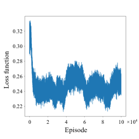
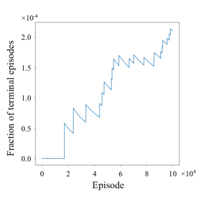
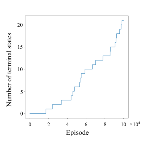
Figure 7: Learning results for the quark sector. The results are the output of neural network leading to the best-fit model shown in Table 5. From left to right, three panels show (a) the loss function vs episode number (b) the fraction of terminal episodes vs episode number (c) the number of terminal states vs episode number, respectively.

Charges	${\cal Q}=\left(\begin{array}[]{ccc|ccc|ccc|cc}Q_{1}&Q_{2}&Q_{3}&u_{1}&u_{2}&u_{3}&d_{1}&d_{2}&d_{3}&H&\phi\\ \hline\cr 9&8&6&1&3&4&6&5&5&-2&1\\ \end{array}\right)$
$\mathcal{O}\left(1\right)$ coeff.	$y^{u}\simeq\left(\begin{array}[]{rrr}0.430&0.806&-1.220\\ -0.962&-0.598&-0.747\\ -1.328&-1.172&1.018\end{array}\right)\ ,\ y^{d}\simeq\left(\begin{array}[]{rrr}-0.996&-0.747&-1.068\\ 0.958&1.441&1.033\\ 0.765&-0.500&-1.029\end{array}\right)$
VEV	$v_{\phi}\simeq 0.181\cdot e^{-0.863i}$
Intrinsic value	$\mathcal{V}_{\mathrm{opt}}\simeq-0.701$
Masses (output)	$\left(\begin{array}[]{lll}m_{u}&m_{c}&m_{t}\\ m_{d}&m_{s}&m_{b}\end{array}\right)\simeq\left(\begin{array}[]{lll}0.002&1.468&180.945\\ 0.003&0.102&4.501\end{array}\right)\ \mathrm{GeV}$
Ratios (masses)	$\left(\begin{array}[]{lll}E_{u}&E_{c}&E_{t}\\ E_{d}&E_{s}&E_{b}\end{array}\right)\simeq\left(\begin{array}[]{lll}0.008&0.063&0.020\\ 0.149&0.037&0.032\end{array}\right)$
CKM matrix (output)	$\left|V_{\mathrm{CKM}}\right|\simeq\left(\begin{array}[]{lll}0.973&0.229&0.004\\ 0.229&0.972&0.057\\ 0.009&0.057&0.998\end{array}\right)$
Ratios (mixings)	$E_{\cal C}\simeq\left(\begin{array}[]{lll}0.000&0.005&0.047\\ 0.004&0.001&0.149\\ 0.033&0.152&0.000\end{array}\right)$

Table 5: Benchmark point for the quark sector.

5 Learning the neutrino structure

In this section, we move to the numerical analysis of the lepton sector, following the RL with DQN introduced in the Secs. 2 and 3. Based on the analysis in Sec. 4, we fix the Higgs $U(1)$ charges and the VEV $v_{\phi}$ to realize the 21 realistic FN models in the quark sector. However, there still exists $19^{9}\sim 3.2\times 10^{11}$ possible states within the range of $U(1)$ charges $-9\leq q\leq 9$ in the environment. We first analyze the lepton sector with fixed neutrino mass ordering; normal ordering or inverted ordering in Sec. 5.1. In the next analysis of Sec. 5.2, the neutrino mass ordering has not been fixed yet. Thus, one can find plausible FN models whether the neutrino masses are in the normal ordering or in the inverted ordering.

5.1 Fixed ordering of neutrino masses

By training the neural network about 8 hours on a single CPU, it turned out that terminal states are found after ${\cal O}(5,000)$ episodes as shown in Fig. 8 with the normal ordering. The loss function tends to be minimized as in Fig. 8 until ${\cal O}(50,000)$ episodes. It is notable that the reward increases when the loss function decreases. After these critical numbers of episodes, the loss function increases, indicating a sign of overtraining. This is because the lepton sector rapidly leads to the terminal states compared with the quark sector. Indeed, the network leads to terminal states in ¿0.06% of all cases for total episode $N_{\rm ep}=6\times 10^{4}$. Therefore, for the lepton sector, we provided an upper bound for the computational cost, which is that ${\cal O}(50,000)$ episodes are sufficient for the agent to acquire the optimal behavior. After removing the negative integers of $n_{ij}$ in Eq. (3.4) and picking up flavon $U(1)$ charge to be consistent with quark sector, we arrive at 63 and 121 terminal states with normal ordering and inverted ordering, respectively. By performing the Monte-Carlo search over the ${\cal O}(1)$ coefficients $y_{ij}$ with the Gaussian distribution shown in Fig. 6, the lepton masses and mixings are further optimized to more realistic ones, according to which the intrinsic value is also optimized. Specifically, we performed the Monte-Carlo search 10 times to search the realistic values within $3\sigma$. In the first 10,000 trials, the ${\cal O}(1)$ coefficients $y_{ij}$ are optimized by using the Gaussian distribution shown in Fig. 6. Then, for the ${\cal O}(1)$ coefficients with highest intrinsic value among them, we performed the second 10,000 trials with the Gaussian distribution where an average is the coefficients obtained by the first Monte-Carlo search and the standard deviation is 0.25.

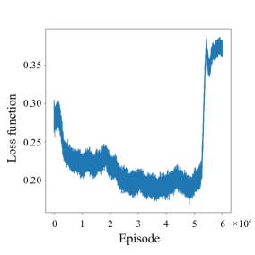
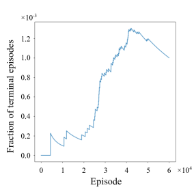
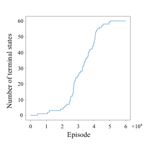
Figure 8: Learning results for the lepton sector with fixed NO of neutrino masses. The results are the output of neural network leading to the best-fit model (the square in Figs. 9 and 10). From left to right, three panels show (a) the loss function vs episode number (b) the fraction of terminal episodes vs episode number (c) the number of terminal states vs episode number, respectively.

After carrying out the same procedure 10 times in total, we find that the results of 6 models with normal ordering are in agreement with experimental values within $3\sigma$. We show the benchmark point with the highest intrinsic value in Table 6 for the normal ordering. Here, we list the effective Majorana neutrino mass $m_{\beta\beta}$ for the neutrinoless double beta decay:

$$m_{\beta\beta}=\left|m_{1}\cos^{2}{\theta_{12}}\cos^{2}{\theta_{13}}+m_{2}\sin^{2}{\theta_{12}}\cos^{2}{\theta_{13}}e^{i\alpha_{21}}+m_{3}\sin^{2}{\theta_{13}}e^{i(\alpha_{31}-2\delta_{\mathrm{CP}})}\right|,$$ (5.1)

which would be measured by the KamLAND-Zen experiment KamLAND-Zen:2022tow . In this analysis, we assume the parameter $M=10^{15}$ GeV to realize the tiny neutrino masses with ${\cal O}(1)$ coefficients of Yukawa couplings, but we leave the detailed study with different values of $M$ for future work. Note that the angular component of flavon leads to the nonvanishing Majorana CP phases in contrast to the quark sector. Thus, one can analyze the correlation between mixing angles and CP phase as shown in Figs. 9 and 10 for the normal ordering, in which all the terminal states within $3\sigma$ are shown. The CP phase $\alpha_{21}$ is predicted at 0. Note that the information of the CP phase has not been implemented in the learning of neural network.

Remarkably, one cannot find the neutrino mass of inverted ordering to be consistent with the experimental values within $3\sigma$, although we perform the Monte-Carlo search 10 times over the ${\cal O}(1)$ coefficients $y_{ij}$ of 121 terminal states. It indicates that normal ordering will be favored by the autonomous behavior of the agent. Indeed, the intrinsic value of normal ordering after the Monte-Carlo search tends to be larger than that of inverted ordering as shown in Fig. 11.

Charges	${\cal Q}=\left(\begin{array}[]{ccc|ccc|ccc|cc}L_{1}&L_{2}&L_{3}&N_{1}&N_{2}&N_{3}&l_{1}&l_{2}&l_{3}&H&\phi\\ \hline\cr 2&1&2&-8&-1&-9&-7&-3&-3&-1&1\\ \end{array}\right)$
$\mathcal{O}\left(1\right)$ coeff.	$y^{l}\simeq\left(\begin{array}[]{rrr}-0.889&2.056&-0.299\\ -1.584&-2.697&1.542\\ -0.797&0.918&1.501\end{array}\right)\ ,\ y^{\nu}\simeq\left(\begin{array}[]{rrr}1.135&-1.331&0.128\\ 1.207&-1.203&-0.051\\ -0.671&-2.639&0.074\end{array}\right)$
	$y^{N}\simeq\left(\begin{array}[]{rrr}1.125&-0.388&0.950\\ -0.388&1.066&-0.349\\ 0.950&-0.349&-0.656\end{array}\right)$
VEV	$v_{\phi}\simeq 0.268\cdot e^{-0.166i}$
Intrinsic value	$\mathcal{V}_{\mathrm{opt}}\simeq-0.853$
Masses (output)	$\left(\begin{array}[]{lll}m_{e}&m_{\mu}&m_{\tau}\end{array}\right)\simeq\left(\begin{array}[]{lll}4.576\times 10^{-1},&1.231\times 10^{2},&7.571\times 10^{2}\end{array}\right)\ \mathrm{MeV}$ $\left(\begin{array}[]{lll}m_{\nu_{1}}&m_{\nu_{2}}&m_{\nu_{3}}\end{array}\right)\simeq\left(\begin{array}[]{lll}0.107,&8.500,&49.39\end{array}\right)\ \mathrm{meV}$
Ratios (masses)	$\left(\begin{array}[]{lll}E_{e}&E_{\mu}&E_{\tau}\\ E_{\nu_{21}}&E_{\nu_{31}}&\end{array}\right)\simeq\left(\begin{array}[]{lll}0.048&0.066&0.371\\ 0.011&0.012&\end{array}\right)$
PMNS matrix (output)	$\left|V_{\mathrm{PMNS}}\right|\simeq\left(\begin{array}[]{lll}0.819&0.553&0.154\\ 0.346&0.689&0.637\\ 0.458&0.468&0.756\end{array}\right)$
Ratios (mixings)	$E_{\cal P}\simeq\left(\begin{array}[]{lll}0.003&0.006&0.013\\ 0.030&0.062&0.041\\ 0.064&0.088&0.038\end{array}\right)$
Majorana phases	$\alpha_{21}\simeq 0.0,\ \alpha_{31}\simeq-0.106\pi$
Effective mass	$m_{\beta\beta}\simeq 3.793\ \mathrm{meV}$

Table 6: Benchmark point for the lepton sector with NO, where the neutrino mass ordering is specified in the learning of the network.

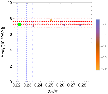
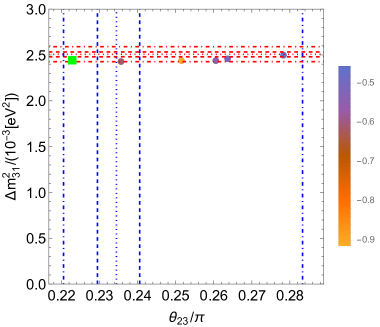
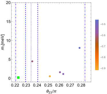
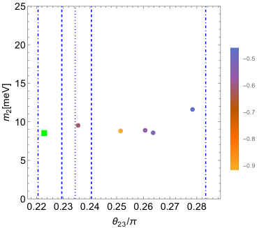
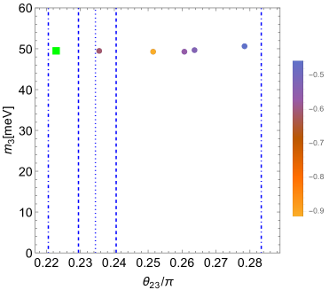
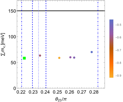
Figure 9: Neutrino masses vs mixing angle $\theta_{23}$, where the dotted line represents the global best fit value in NuFIT v5.2 results with Super-Kamiokande atmospheric data Esteban:2020cvm , and the inside region of each line represents dashed line $\leq 1\sigma$, dotdashed line $\leq 3\sigma$ CL, respectively. The sum of neutrino masses is constrained by $0.15$ eV (95% CL) corresponding to the black solid line in the case of $\Lambda$CDM model RoyChoudhury:2019hls . We denote a best-fit point within $3\sigma$ by a square, and the intrinsic value (3.14) is written in the legend. Note that the neutrino mass ordering is fixed as NO in the training of the neural network.

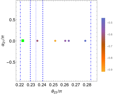
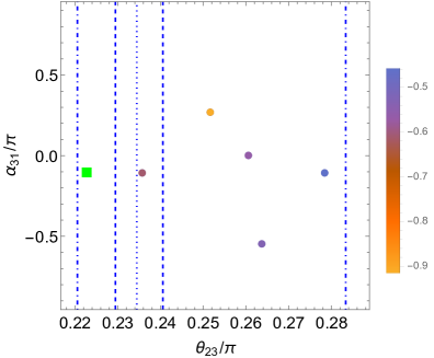
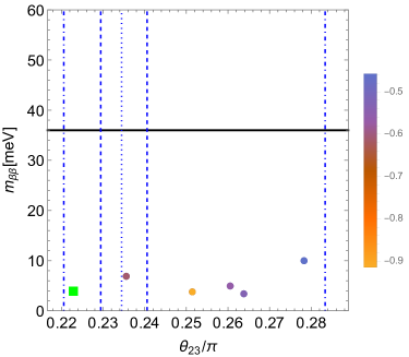
Figure 10: Majorana phases $\alpha_{21},\alpha_{31}$ and effective Majorana neutrino mass $m_{\beta\beta}$ vs mixing angle $\theta_{23}$, where the dotted line represents the global best fit value in NuFIT v5.2 results with Super-Kamiokande atmospheric data Esteban:2020cvm , and the inside region of each line represents dashed line $\leq 1\sigma$, dotdashed line $\leq 3\sigma$ CL, respectively. The effective Majorana neutrino mass is upper bounded by $0.036$ eV (90% CL) corresponding to the black solid line KamLAND-Zen:2022tow . We denote a best-fit point within $3\sigma$ by a square, and the intrinsic value (3.14) is written in the legend. Note that the neutrino mass ordering is fixed as NO in the training of the neural network.

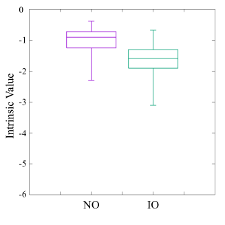
(a) Only lepton sector.

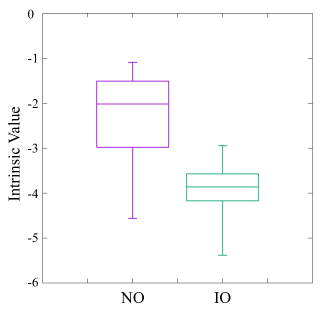
(b) Sum with quark sector.

Figure 11: Boxplots of intrinsic values for the lepton sector, where the neutrino mass ordering is fixed in the learning of neural network. In the left panel, we show intrinsic values obtained in the RL with the lepton sector, but in the right panel, we incorporate the values of the quark sector analyzed in Sec. 4.

5.2 Unfixed ordering of neutrino masses

In this subsection, we train the neural network without specifying the neutrino mass ordering. For each of the 21 realistic FN models in the quark sector, we performed the training twice to obtain a sufficient number of realistic models. Similar to the previous analyses, the neural network is trained about 12 hours on a single CPU. It turned out that terminal states are found after ${\cal O}(2,000)$ episodes as shown in Fig. 12, where the loss function tends to decrease until ${\cal O}(8,000)$ episodes. It is notable that the reward increases when the loss function decreases, and the lepton sector rapidly leads to the terminal states compared with the quark sector. The network leads to terminal states in about ¿60% of all cases for total episode $N_{\rm ep}=6\times 10^{4}$. In contrast to the previous analysis, the trained network efficiently leads to terminal states. After removing the negative integers of $n_{ij}$ in Eq. (3.4), we arrive at 13,733 (13,432) and 22,430 (20,357) terminal states with normal ordering and inverted ordering in the first (second) learning, respectively . By performing the Monte-Carlo search over the ${\cal O}(1)$ coefficients $y_{ij}$ with the Gaussian distribution shown in Fig. 6, the lepton masses and mixings are optimized to more realistic ones, according to which the intrinsic value is also optimized. Specifically, we performed the Monte-Carlo search two times to search the realistic values within $3\sigma$. In the first Monte-Carlo search, we ran 10,000 trials with the Gaussian distribution shown in Fig. 6. Then, for the ${\cal O}(1)$ coefficients with highest intrinsic value among them, we performed the second 10,000 trials with the Gaussian distribution where an average is the coefficients obtained by the first Monte-Carlo search and the standard deviation is 0.25.

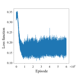
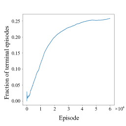
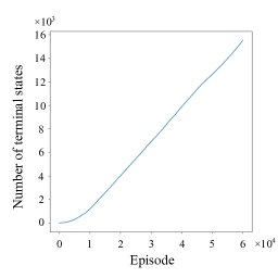
Figure 12: Learning results for the lepton sector by RL without specifying the neutrino mass ordering. The results are the output of neural network leading to the best-fit model (the diamond in Figs. 13 and 14). We observe a similar behavior for other outputs. From left to right, three panels show (a) the loss function vs episode number (b) the fraction of terminal episodes vs episode number (c) the number of terminal states vs episode number, respectively.

After carrying out the Monte-Carlo analysis, we find that the results of 15 models with normal ordering are in agreement with experimental values within $3\sigma$. Two best fit points with the highest intrinsic value are shown in Tables 7 and 8 for the normal ordering. As presented in the previous section, one can analyze the correlation between mixing angles and the other observed values as shown in Figs. 13 and 14 for the normal ordering, in which all the terminal states within $3\sigma$ are shown. It turned out that the Majorana CP phases are typically nonzero, and the summation of neutrino masses and the effective mass are not widely distributed but tend to be localized at $\sum_{i}m_{\nu_{i}}\sim 60\,{\rm meV}$ and $2\,{\rm meV}\leq m_{\beta\beta}\leq 6\,{\rm meV}$, respectively.

Charges	${\cal Q}=\left(\begin{array}[]{ccc|ccc|ccc|cc}L_{1}&L_{2}&L_{3}&N_{1}&N_{2}&N_{3}&l_{1}&l_{2}&l_{3}&H&\phi\\ \hline\cr 3&3&2&-3&0&0&-3&0&0&-2&1\\ \end{array}\right)$
$\mathcal{O}\left(1\right)$ coeff.	$y^{l}\simeq\left(\begin{array}[]{rrr}1.728&-1.717&1.790\\ 1.225&-0.456&-1.589\\ -2.243&-2.316&-2.664\end{array}\right)\ ,\ y^{\nu}\simeq\left(\begin{array}[]{rrr}-1.737&-1.060&2.712\\ 3.083&-1.698&-0.342\\ -0.396&0.9445&-0.287\end{array}\right)$
	$y^{N}\simeq\left(\begin{array}[]{rrr}-1.031&2.275&1.453\\ 2.275&-0.457&0.333\\ 1.453&0.333&1.559\end{array}\right)$
VEV	$v_{\phi}\simeq 0.181\cdot e^{-0.863i}$
Intrinsic value	$\mathcal{V}_{\mathrm{opt}}\simeq-0.859$
Masses (output)	$\left(\begin{array}[]{lll}m_{e}&m_{\mu}&m_{\tau}\end{array}\right)\simeq\left(\begin{array}[]{lll}4.960\times 10^{-1},&8.575\times 10^{1},&6.553\times 10^{2}\end{array}\right)\ \mathrm{MeV}$ $\left(\begin{array}[]{lll}m_{\nu_{1}}&m_{\nu_{2}}&m_{\nu_{3}}\end{array}\right)\simeq\left(\begin{array}[]{lll}0.210,&8.869,&50.18\end{array}\right)\ \mathrm{meV}$
Ratios (masses)	$\left(\begin{array}[]{lll}E_{e}&E_{\mu}&E_{\tau}\\ E_{\nu_{21}}&E_{\nu_{31}}&\end{array}\right)\simeq\left(\begin{array}[]{lll}0.013&0.091&0.433\\ 0.026&0.002&\end{array}\right)$
PMNS matrix (output)	$\left|V_{\mathrm{PMNS}}\right|\simeq\left(\begin{array}[]{lll}0.823&0.548&0.149\\ 0.332&0.677&0.656\\ 0.460&0.491&0.740\end{array}\right)$
Ratios (mixings)	$E_{\cal P}\simeq\left(\begin{array}[]{lll}0.000&0.001&0.001\\ 0.048&0.054&0.028\\ 0.066&0.067&0.029\end{array}\right)$
Majorana phases	$\alpha_{21}\simeq 0.0,\ \alpha_{31}\simeq 0.549\pi$
Effective mass	$m_{\beta\beta}\simeq 2.850\ \mathrm{meV}$

Table 7: Benchmark point for the lepton sector with NO (corresponding to the diamond in Figs. 13 and 14), where the neutrino mass ordering is not specified in the learning of the network.

Charges	${\cal Q}=\left(\begin{array}[]{ccc|ccc|ccc|cc}L_{1}&L_{2}&L_{3}&N_{1}&N_{2}&N_{3}&l_{1}&l_{2}&l_{3}&H&\phi\\ \hline\cr 2&3&1&-7&-8&-1&-2&-5&-1&-1&1\\ \end{array}\right)$
$\mathcal{O}\left(1\right)$ coeff.	$y^{l}\simeq\left(\begin{array}[]{rrr}-0.424&-0.567&0.897\\ -0.482&-0.787&0.827\\ 0.141&-0.704&0.565\end{array}\right)\ ,\ y^{\nu}\simeq\left(\begin{array}[]{rrr}-1.243&1.096&0.396\\ -0.898&-1.501&-3.224\\ 2.361&2.246&-1.668\end{array}\right)$
	$y^{N}\simeq\left(\begin{array}[]{rrr}2.311&0.877&-1.491\\ 0.877&-1.746&0.186\\ -1.491&0.186&-0.283\end{array}\right)$
VEV	$v_{\phi}\simeq 0.268\cdot e^{-0.166i}$
Intrinsic value	$\mathcal{V}_{\mathrm{opt}}\simeq-0.720$
Masses (output)	$\left(\begin{array}[]{lll}m_{e}&m_{\mu}&m_{\tau}\end{array}\right)\simeq\left(\begin{array}[]{lll}4.067\times 10^{-1},&1.483\times 10^{2},&2.066\times 10^{3}\end{array}\right)\ \mathrm{MeV}$ $\left(\begin{array}[]{lll}m_{\nu_{1}}&m_{\nu_{2}}&m_{\nu_{3}}\end{array}\right)\simeq\left(\begin{array}[]{lll}2.251,&9.006,&50.04\end{array}\right)\ \mathrm{meV}$
Ratios (masses)	$\left(\begin{array}[]{lll}E_{e}&E_{\mu}&E_{\tau}\\ E_{\nu_{21}}&E_{\nu_{31}}&\end{array}\right)\simeq\left(\begin{array}[]{lll}0.099&0.147&0.066\\ 0.011&0.000&\end{array}\right)$
PMNS matrix (output)	$\left|V_{\mathrm{PMNS}}\right|\simeq\left(\begin{array}[]{lll}0.817&0.556&0.151\\ 0.499&0.552&0.668\\ 0.288&0.621&0.729\end{array}\right)$
Ratios (mixings)	$E_{\cal P}\simeq\left(\begin{array}[]{lll}0.004&0.008&0.005\\ 0.129&0.035&0.020\\ 0.137&0.035&0.023\end{array}\right)$
Majorana phases	$\alpha_{21}\simeq 0.106\pi,\ \alpha_{31}\simeq-0.211\pi$
Effective mass	$m_{\beta\beta}\simeq 5.040\ \mathrm{meV}$

Table 8: Benchmark point for the lepton sector with NO (corresponding to the square in Figs. 13 and 14), where the neutrino mass ordering is not specified in the learning of the network.

Remarkably, one cannot obtain the experimental values of neutrino masses and mixings within $3\sigma$ for the inverted ordering, although we perform the Monte-Carlo searches over the ${\cal O}(1)$ coefficients $y_{ij}$ of all the terminal states. Thus, the normal ordering of neutrino masses is also favored by the trained neural network, although the neural network itself was trained without any knowledge of neutrino mass ordering. Indeed, the intrinsic value of normal ordering after the Monte-Carlo search tends to be larger than that of inverted ordering as shown in Fig. 15. This conspicuous feature can also be seen by looking at the intrinsic value including both the quark and lepton sectors.

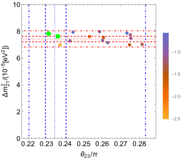
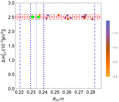
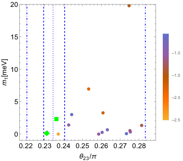
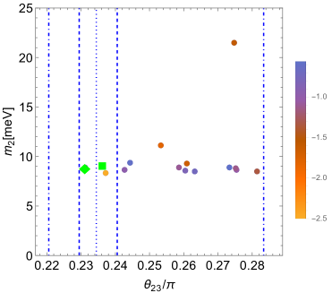
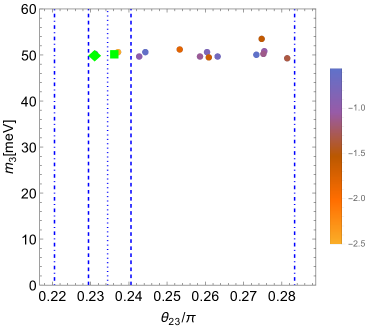
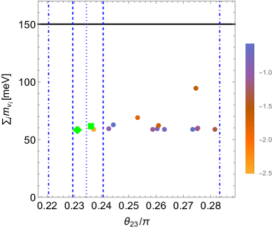
Figure 13: Neutrino masses vs mixing angle $\theta_{23}$, where the dotted line represents the global best fit value in NuFIT v5.2 results with Super-Kamiokande atmospheric data Esteban:2020cvm , and the inside region of each line represents dashed line $\leq 1\sigma$, dotdashed line $\leq 3\sigma$ CL, respectively. The sum of neutrino masses is constrained by $0.15$ eV (95% CL) corresponding to the black solid line in the case of $\Lambda$CDM model RoyChoudhury:2019hls . We denote two best-fit points within $3\sigma$ by a diamond and a square, and the intrinsic value (3.14) is written in the legend. Since the neutrino mass ordering is unfixed in the training of the neural network, we show only NO results from the terminal states.

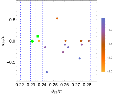
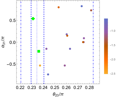
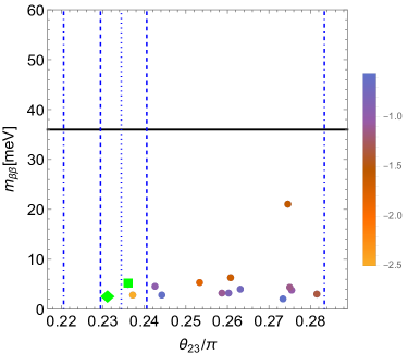
Figure 14: Majorana phases $\alpha_{21},\alpha_{31}$ and effective Majorana neutrino mass $m_{\beta\beta}$ vs mixing angle $\theta_{23}$, where the dotted line represents the global best fit value in NuFIT v5.2 results with Super-Kamiokande atmospheric data Esteban:2020cvm , and the inside region of each line represents dashed line $\leq 1\sigma$, dotdashed line $\leq 3\sigma$ CL, respectively. The effective Majorana neutrino mass is upper bounded by $0.036$ eV (90% CL) corresponding to the black solid line KamLAND-Zen:2022tow . We denote two best-fit points within $3\sigma$ by a diamond and a square, and the intrinsic value (3.14) is written in the legend.

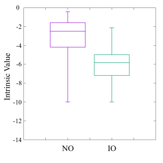
(a) Only the lepton sector.

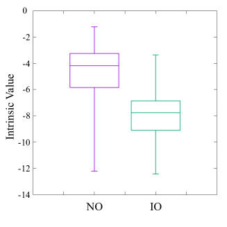
(b) Both the lepton and quark sectors.

Figure 15: Boxplots of intrinsic values for the lepton sector from the result of second learning, where the neutrino mass ordering is unspecified in the learning of neural network. In the left panel, we show intrinsic values obtained in the RL with the lepton sector, but in the right panel, we incorporate the values of the quark sector analyzed in Sec. 4. We obtain similar results in the first learning.

6 Conclusion

The flavor symmetries are one of attractive tools to understand the flavor structure of quarks and leptons. To address the flavor puzzle in the Standard Model, we have applied the reinforcement learning technique to flavor models with $U(1)$ horizontal symmetry. RL will shed new light on the phenomenological approach to scan over the parameter space of flavor models in contrast to the brute-force approach.

In this paper, we have extended the analysis of Ref. Harvey:2021oue to explore the flavor structure of quarks and leptons by employing the RL with DQN. Based on the neural network architectures in the framework of $U(1)$ flavor model with RL established in Secs. 2 and 3, the agent is designed to exhibit autonomous behavior in the environment (parameter space of $U(1)$ charges). Since the parameter space of $U(1)$ charges is huge, we have performed a separate search for the $U(1)$ charge assignment of quarks and leptons. Trained neural network leads to phenomenologically promising terminal states in ¿6% for the quark sector and ¿60% for the lepton sector in the case of unfixed ordering of neutrino masses. In the analysis of Sec. 5.2, we have not specified the neutrino mass ordering in the evaluation of intrinsic value, meaning that the agent does not have any knowledge of neutrino mass ordering. However, the autonomous behavior of the agent suggests us that the intrinsic value of normal ordering tends to be larger than that of inverted ordering as shown in Fig. 15, and the normal ordering is well fitted with the current experimental data in contrast to the inverted ordering. Remarkably, the effective mass for the neutrinoless double beta decay is predicted around specific values, and the Majorana CP phases are nonzero in general.

Before closing our paper, it is worthwhile mentioning a possible application of our analysis:

• We have focused on the flavor structure of Yukawa couplings, but it is easily applicable to reveal the flavor structure of higher-dimensional operators (see for the Standard Model effective field theory (SMEFT) with $U(1)$ flavor symmetry Bordone:2019uzc and discrete symmetry Kobayashi:2021pav .). Since the trained neural network predicts the plausible charge assignment of quarks and leptons, one can also determine the flavor structure of higher-dimensional operators. It would be interesting to clarify whether RL technique we proposed can explore the flavor structure of the SMEFT.

• On top of that, the CP-odd fluctuation of complex flavon field (flaxion) would be regarded as QCD axion as discussed in Refs. Salvio:2015cja ; Ballesteros:2016euj ; Ballesteros:2016xej ; Ema:2016ops , where the cosmological problems (such as the origin of dark matter, baryon asymmetry of the Universe, and the inflation) are simultaneously solved by the dynamics of flavon field. Since the flavon field has flavor changing neutral current (FCNC) interactions with quarks and leptons controlled by the $U(1)$ flavor symmetry, charge assignment of quarks and leptons plays an important role of determining the FCNC processes. It is fascinating to apply our finding charge assignment to such an axion physics, which left for future work.

• We have focused on the $U(1)$ horizontal symmetry, but it is easily applicable to other flavor symmetries such as discrete flavor symmetries. We hope to elucidate a comprehensive study about the global structure of flavor models in an upcoming paper.

• By analyzing the underlying factors that characterize reasonable flavor models from neural networks, we will figure out general patterns behind the flavor models. The search for the flavor structure by RL is expected not only to explore new physics beyond the Standard Model by validating flavor models, but also to unravel the black box of machine learning itself.

Appendix A Formulation of reinforcement learning

This Appendix provides a brief review about the formulation of RL. Note that the notation used here is independent of that in the main text. In the following, we denote the state space $\mathcal{S}$ and the action space $\mathcal{A}$, respectively.

The most fundamental assumption in RL is to utilize the Markov Decision Processes (MDPs) for solving the problem. MDPs are state transitions in which the state $s_{t}$ and reward $r_{t}$ at time $t$ are completely determined by the state $s_{t-1}$ and action $a_{t-1}$ at the previous time $t-1$.

Considering a specific policy $\pi\left(\mathfrak{a}|s\right)$ under the MDPs, the total reward $R_{t}$, the state-value function $V\left(s\right)$ and the action-value function $Q\left(s,\mathfrak{a}\right)$ are defined as follows:

$$R_{t} =\sum_{t^{\prime}=0}^{\infty}\gamma^{t^{\prime}}r_{t+t^{\prime}},$$ (A.1)

$$V^{\pi}\left(s\right) =\mathbb{E}\left[R_{t};s_{t}=s\right],$$ (A.2)

$$Q^{\pi}\left(s,\mathfrak{a}\right) =\mathbb{E}\left[R_{t};s_{t}=s,\mathfrak{a}_{t}=\mathfrak{a}\right],$$ (A.3)

where $\mathbb{E}$ means an expected value. Note that the discount rate $\gamma$ is a real number satisfying $0<\gamma<1$, and it weights the rewards at each time to prevent divergence of the values. These equations define the value functions as the expected value of the total reward that could be obtained at times after $t$. The relation between $V\left(s\right)$ and $Q\left(s,\mathfrak{a}\right)$ is as follows:

$$V^{\pi}\left(s\right)=\sum_{\mathfrak{a}\in\mathcal{A}}\pi\left(\mathfrak{a}|s\right)Q^{\pi}\left(s,\mathfrak{a}\right).$$ (A.4)

The goal of RL is to determine an optimal policy $\pi^{*}$ that maximizes the expected value of $R_{t}$. This is equivalent to deriving $\pi^{*}$ such that $V\left(s\right)$ and $Q\left(s,\mathfrak{a}\right)$ are maximized. To solve this optimization problem, we first rewrite Eq.(A.2) (the definition of $V\left(s\right)$) into a recursive expression as follows:

$$V^{\pi}\left(s\right) =\mathbb{E}\left[r_{t}+\gamma\sum_{t^{\prime}=1}^{\infty}\gamma^{t^{\prime}-1}r_{t+t^{\prime}};s_{t}=s\right]$$ (A.5)

$$=\sum_{\mathfrak{a}\in\mathcal{A}}\pi\left(\mathfrak{a}|s\right)\sum_{s^{\prime}\in\mathcal{S}}p\left(s^{\prime}|s,\mathfrak{a}\right)\left[r_{t}+\gamma V^{\pi}\left(s^{\prime}\right)\right].$$ (A.6)

Here, $p\left(s^{\prime}|s,\mathfrak{a}\right)$ is the probability distribution for “choosing the action $\mathfrak{a}_{t}$ in state $s_{t}$, and transition to state $s_{t+1}$”, which completely characterizes the time evolution of the environment under MDPs. The similar deformation for Eq.(A.3) (the definition of $Q\left(s,\mathfrak{a}\right)$) leads to the following equation:

$$Q^{\pi}\left(s,\mathfrak{a}\right)=\sum_{s^{\prime}\in\mathcal{S}}p\left(s^{\prime}|s,\mathfrak{a}\right)\left[r_{t}+\gamma\sum_{\mathfrak{a^{\prime}}\in\mathcal{A}}\pi\left(\mathfrak{a^{\prime}}|s^{\prime}\right)Q^{\pi}\left(s^{\prime},\mathfrak{a^{\prime}}\right)\right].$$ (A.7)

These equations represent the expected reward obtained under a specific policy $\pi$. On the other hand, the probability of choosing an action is deterministic if the agent has acquired the optimal policy $\pi^{*}$. That is, the probability of taking a particular action is 1, and 0 otherwise. This makes the optimal solutions $\{V^{*},Q^{*}\}$ satisfy the following equations:

$$V^{*}\left(s\right) =\max_{\mathfrak{a}\in\mathcal{A}}\sum_{s^{\prime}\in\mathcal{S}}p\left(s^{\prime}|s,\mathfrak{a}\right)\left[r_{t}+\gamma V^{*}\left(s^{\prime}\right)\right],$$ (A.8)

$$Q^{*}\left(s,\mathfrak{a}\right) =\sum_{s^{\prime}\in\mathcal{S}}p\left(s^{\prime}|s,\mathfrak{a}\right)\left[r_{t}+\gamma\max_{\mathfrak{a^{\prime}}\in\mathcal{A}}Q^{*}\left(s^{\prime},\mathfrak{a^{\prime}}\right)\right].$$ (A.9)

These recursive equations are called as Bellman equations. When the state transition probability $p\left(s^{\prime}|s,\mathfrak{a}\right)$ is known, the equations can be solved by the sequential assignment method. In reality, however, complete information on $p\left(s^{\prime}|s,\mathfrak{a}\right)$ is rarely known. Furthermore, even if the state-value $V$ is calculated without such information, the expected value of rewards from a particular action cannot be calculated, so an appropriate action cannot be determined. Therefore, in many realistic problems, the action-value $Q$ is approximated by some mathematical models such as a neural network, and parameters are determined so that $Q$ is maximized. This method is called as the value-based approach.

Rewriting Eq.(A.9) based on the sequential assignment method, we obtain the following expression where $\alpha$ is the learning rate:

$$Q\left(s,\mathfrak{a}\right)\leftarrow Q\left(s,\mathfrak{a}\right)+\alpha\left[r\left(s,\mathfrak{a}\right)+\gamma\sum_{s^{\prime}\in\mathcal{S}}p\left(s^{\prime}|s,\mathfrak{a}\right)\max_{\mathfrak{a^{\prime}}\in\mathcal{A}}Q\left(s^{\prime},\mathfrak{a^{\prime}}\right)-Q\left(s,\mathfrak{a}\right)\right].$$ (A.10)

The expected reward $r\left(s,\mathfrak{a}\right)$ is defined as:

$$r\left(s,\mathfrak{a}\right)=\sum_{s^{\prime}\in\mathcal{S}}p\left(s^{\prime}|s,\mathfrak{a}\right)r_{t}.$$ (A.11)

When the concrete expression of $p\left(s^{\prime}|s,\mathfrak{a}\right)$ is not known, first, the action $\mathfrak{a}$ is selected based on the currently expected action-value. Next, the maximized action-value is achieved by minimizing the difference from the actually obtained action-value. In this process, $Q\left(s_{t},\mathfrak{a}_{t}\right)$ is updated as follows, and this method of learning is called as Q learning:

$$Q\left(s_{t},\mathfrak{a}_{t}\right)\leftarrow Q\left(s_{t},\mathfrak{a}_{t}\right)+\alpha\left[r_{t}+\gamma\max_{\mathfrak{a}\in\mathcal{A}}Q\left(s_{t+1},\mathfrak{a}\right)-Q\left(s_{t},\mathfrak{a}_{t}\right)\right].$$ (A.12)

In DQN, the term $\max_{\mathfrak{a}\in\mathcal{A}}Q\left(s_{t+1},\mathfrak{a}\right)$ is approximated by the neural network. The action-value is normalized by using a softmax function in the final layer of the neural network. Then, the output value can also be interpreted as probabilities. This allows the output of the neural network to be interpreted as a probability indicating which action is most plausible. In addition, DQN uses Q network (with parameters $\Theta$) and target network (with parameters $\Theta^{\prime}$) to update the action-value as follows to improve the stability of learning:

$$Q_{\Theta}\left(s_{t},\mathfrak{a}_{t}\right)\leftarrow Q_{\Theta}\left(s_{t},\mathfrak{a}_{t}\right)+\alpha\left[r_{t}+\gamma\max_{\mathfrak{a}\in\mathcal{A}}Q_{\Theta^{\prime}}\left(s_{t+1},\mathfrak{a}\right)-Q_{\Theta}\left(s_{t},\mathfrak{a}_{t}\right)\right].$$ (A.13)

Appendix B FN charges

We list our finding charge assignment of quarks in Appendix B.1. For the lepton sector, we present the results of RL by picking the models up only when theoretical values of neutrinos with the normal ordering are within $3\sigma$ considering $(\Delta m_{21}^{2},\Delta m_{31}^{2},\sin^{2}\theta_{12},\sin^{2}\theta_{13},\sin^{2}\theta_{23})$. These are summarized in Appendices B.2 and B.3, where the neutrino mass ordering is specified and unspecified in the learning of neural networks, respectively.

B.1 Quark sector

Charges	${\cal Q}=\left(\begin{array}[]{ccc|ccc|ccc|cc}Q_{1}&Q_{2}&Q_{3}&u_{1}&u_{2}&u_{3}&d_{1}&d_{2}&d_{3}&H&\phi\\ \hline\cr 0&-2&3&1&7&1&8&9&7&-2&-1\\ \end{array}\right)$
$\mathcal{O}\left(1\right)$ coeff.	$y^{u}\simeq\left(\begin{array}[]{rrr}0.856&1.537&0.895\\ -1.071&0.833&-1.377\\ 1.181&-1.507&0.805\end{array}\right)\ ,\ y^{d}\simeq\left(\begin{array}[]{rrr}-0.915&1.347&-0.746\\ -0.559&1.108&0.884\\ 0.898&1.056&1.111\end{array}\right)$
VEV, Value	$v_{\phi}\simeq 0.294\cdot e^{-0.930i}\ ,\ \mathcal{V}_{\mathrm{opt}}\simeq-1.834$
Charges	${\cal Q}=\left(\begin{array}[]{ccc|ccc|ccc|cc}Q_{1}&Q_{2}&Q_{3}&u_{1}&u_{2}&u_{3}&d_{1}&d_{2}&d_{3}&H&\phi\\ \hline\cr-7&-9&-4&-6&-5&-7&3&4&2&-3&-1\\ \end{array}\right)$
$\mathcal{O}\left(1\right)$ coeff.	$y^{u}\simeq\left(\begin{array}[]{rrr}-1.001&-0.857&0.989\\ 0.791&0.868&0.889\\ -0.889&-0.885&-0.940\end{array}\right)\ ,\ y^{d}\simeq\left(\begin{array}[]{rrr}-0.995&0.870&-0.985\\ 1.199&-1.127&-1.412\\ -1.325&-0.882&-1.020\end{array}\right)$
VEV, Value	$v_{\phi}\simeq 0.283\cdot e^{-0.860i}\ ,\ \mathcal{V}_{\mathrm{opt}}\simeq-1.416$
Charges	${\cal Q}=\left(\begin{array}[]{ccc|ccc|ccc|cc}Q_{1}&Q_{2}&Q_{3}&u_{1}&u_{2}&u_{3}&d_{1}&d_{2}&d_{3}&H&\phi\\ \hline\cr-6&-5&-3&5&4&2&-5&-7&-5&5&-1\\ \end{array}\right)$
$\mathcal{O}\left(1\right)$ coeff.	$y^{u}\simeq\left(\begin{array}[]{rrr}-1.451&1.161&-0.722\\ -1.475&0.953&-1.262\\ 0.798&0.865&1.182\end{array}\right)\ ,\ y^{d}\simeq\left(\begin{array}[]{rrr}1.229&-0.976&0.756\\ -1.280&-0.985&-1.159\\ 1.235&0.355&0.825\end{array}\right)$
VEV, Value	$v_{\phi}\simeq 0.171\cdot e^{0.649i}\ ,\ \mathcal{V}_{\mathrm{opt}}\simeq-2.066$
Charges	${\cal Q}=\left(\begin{array}[]{ccc|ccc|ccc|cc}Q_{1}&Q_{2}&Q_{3}&u_{1}&u_{2}&u_{3}&d_{1}&d_{2}&d_{3}&H&\phi\\ \hline\cr-6&-8&-3&3&7&1&-5&-3&-5&4&-1\\ \end{array}\right)$
$\mathcal{O}\left(1\right)$ coeff.	$y^{u}\simeq\left(\begin{array}[]{rrr}1.498&1.767&-1.223\\ 1.090&-1.531&-1.080\\ -1.035&-1.383&-0.864\end{array}\right)\ ,\ y^{d}\simeq\left(\begin{array}[]{rrr}0.778&1.466&0.921\\ -0.945&-0.858&-1.249\\ -1.077&0.555&-1.006\end{array}\right)$
VEV, Value	$v_{\phi}\simeq 0.300\cdot e^{0.912i}\ ,\ \mathcal{V}_{\mathrm{opt}}\simeq-1.881$
Charges	${\cal Q}=\left(\begin{array}[]{ccc|ccc|ccc|cc}Q_{1}&Q_{2}&Q_{3}&u_{1}&u_{2}&u_{3}&d_{1}&d_{2}&d_{3}&H&\phi\\ \hline\cr-3&-2&0&6&3&2&1&-1&0&2&-1\\ \end{array}\right)$
$\mathcal{O}\left(1\right)$ coeff.	$y^{u}\simeq\left(\begin{array}[]{rrr}-0.791&1.769&1.053\\ 1.177&1.045&0.807\\ 1.280&0.924&-0.984\end{array}\right)\ ,\ y^{d}\simeq\left(\begin{array}[]{rrr}1.112&-0.976&0.964\\ -1.332&-0.817&1.121\\ 1.327&-0.774&0.910\end{array}\right)$
VEV, Value	$v_{\phi}\simeq 0.166\cdot e^{-2.199i}\ ,\ \mathcal{V}_{\mathrm{opt}}\simeq-1.584$

Charges	${\cal Q}=\left(\begin{array}[]{ccc|ccc|ccc|cc}Q_{1}&Q_{2}&Q_{3}&u_{1}&u_{2}&u_{3}&d_{1}&d_{2}&d_{3}&H&\phi\\ \hline\cr-5&-4&-2&3&2&0&-1&-2&-1&2&-1\\ \end{array}\right)$
$\mathcal{O}\left(1\right)$ coeff.	$y^{u}\simeq\left(\begin{array}[]{rrr}-0.812&-1.382&1.015\\ 0.949&0.924&-1.598\\ -1.319&-1.511&-0.935\end{array}\right)\ ,\ y^{d}\simeq\left(\begin{array}[]{rrr}-1.129&-0.680&-0.789\\ 0.505&-0.857&-0.994\\ -1.033&-1.134&1.287\end{array}\right)$
VEV, Value	$v_{\phi}\simeq 0.172\cdot e^{1.985i}\ ,\ \mathcal{V}_{\mathrm{opt}}\simeq-1.240$
Charges	${\cal Q}=\left(\begin{array}[]{ccc|ccc|ccc|cc}Q_{1}&Q_{2}&Q_{3}&u_{1}&u_{2}&u_{3}&d_{1}&d_{2}&d_{3}&H&\phi\\ \hline\cr 3&5&0&1&-3&1&-4&-5&-3&1&1\\ \end{array}\right)$
$\mathcal{O}\left(1\right)$ coeff.	$y^{u}\simeq\left(\begin{array}[]{rrr}1.030&-0.155&1.152\\ -0.934&1.382&-0.996\\ -1.349&1.185&-1.036\end{array}\right)\ ,\ y^{d}\simeq\left(\begin{array}[]{rrr}0.323&-1.270&1.333\\ -0.945&1.084&0.987\\ 0.925&-1.042&0.852\end{array}\right)$
VEV, Value	$v_{\phi}\simeq 0.289\cdot e^{-1.223i}\ ,\ \mathcal{V}_{\mathrm{opt}}\simeq-1.405$
Charges	${\cal Q}=\left(\begin{array}[]{ccc|ccc|ccc|cc}Q_{1}&Q_{2}&Q_{3}&u_{1}&u_{2}&u_{3}&d_{1}&d_{2}&d_{3}&H&\phi\\ \hline\cr 1&0&-2&1&-2&2&-8&-8&-8&4&1\\ \end{array}\right)$
$\mathcal{O}\left(1\right)$ coeff.	$y^{u}\simeq\left(\begin{array}[]{rrr}0.999&0.909&-1.021\\ -0.385&1.263&0.820\\ -1.117&0.825&-0.940\end{array}\right)\ ,\ y^{d}\simeq\left(\begin{array}[]{rrr}-1.019&-0.966&-1.312\\ 1.064&0.979&0.800\\ 1.052&0.824&1.242\end{array}\right)$
VEV, Value	$v_{\phi}\simeq 0.173\cdot e^{1.916i}\ ,\ \mathcal{V}_{\mathrm{opt}}\simeq-1.158$
Charges	${\cal Q}=\left(\begin{array}[]{ccc|ccc|ccc|cc}Q_{1}&Q_{2}&Q_{3}&u_{1}&u_{2}&u_{3}&d_{1}&d_{2}&d_{3}&H&\phi\\ \hline\cr-4&-6&-1&5&9&3&-2&-1&-3&4&-1\\ \end{array}\right)$
$\mathcal{O}\left(1\right)$ coeff.	$y^{u}\simeq\left(\begin{array}[]{rrr}1.222&-1.247&1.028\\ -1.169&-1.066&-1.216\\ 1.172&0.916&-1.204\end{array}\right)\ ,\ y^{d}\simeq\left(\begin{array}[]{rrr}-1.021&0.900&0.793\\ 0.804&1.260&0.375\\ -1.029&0.973&0.401\end{array}\right)$
VEV, Value	$v_{\phi}\simeq 0.294\cdot e^{-2.999i}\ ,\ \mathcal{V}_{\mathrm{opt}}\simeq-1.676$

Charges	${\cal Q}=\left(\begin{array}[]{ccc|ccc|ccc|cc}Q_{1}&Q_{2}&Q_{3}&u_{1}&u_{2}&u_{3}&d_{1}&d_{2}&d_{3}&H&\phi\\ \hline\cr-3&-2&0&1&0&-2&3&6&6&-2&-1\\ \end{array}\right)$
$\mathcal{O}\left(1\right)$ coeff.	$y^{u}\simeq\left(\begin{array}[]{rrr}-1.127&-0.701&0.878\\ -1.028&-1.237&-1.274\\ 0.841&0.807&-0.576\end{array}\right)\ ,\ y^{d}\simeq\left(\begin{array}[]{rrr}-1.081&-0.886&-1.166\\ 0.536&1.347&-1.446\\ 0.610&-1.644&-0.976\end{array}\right)$
VEV, Value	$v_{\phi}\simeq 0.184\cdot e^{1.097i}\ ,\ \mathcal{V}_{\mathrm{opt}}\simeq-2.452$
Charges	${\cal Q}=\left(\begin{array}[]{ccc|ccc|ccc|cc}Q_{1}&Q_{2}&Q_{3}&u_{1}&u_{2}&u_{3}&d_{1}&d_{2}&d_{3}&H&\phi\\ \hline\cr-7&-7&-4&6&9&4&-9&-9&-8&8&-1\\ \end{array}\right)$
$\mathcal{O}\left(1\right)$ coeff.	$y^{u}\simeq\left(\begin{array}[]{rrr}1.117&1.057&-0.942\\ -1.244&-0.815&1.181\\ -1.097&0.892&-0.963\end{array}\right)\ ,\ y^{d}\simeq\left(\begin{array}[]{rrr}-1.027&-0.966&-1.200\\ 1.054&0.364&0.947\\ 0.949&-1.305&1.355\end{array}\right)$
VEV, Value	$v_{\phi}\simeq 0.268\cdot e^{1.800i}\ ,\ \mathcal{V}_{\mathrm{opt}}\simeq-1.056$
Charges	${\cal Q}=\left(\begin{array}[]{ccc|ccc|ccc|cc}Q_{1}&Q_{2}&Q_{3}&u_{1}&u_{2}&u_{3}&d_{1}&d_{2}&d_{3}&H&\phi\\ \hline\cr 9&8&6&1&3&4&6&5&5&-2&1\\ \end{array}\right)$
$\mathcal{O}\left(1\right)$ coeff.	$y^{u}\simeq\left(\begin{array}[]{rrr}0.430&0.806&-1.220\\ -0.962&-0.598&-0.747\\ -1.328&-1.172&1.018\end{array}\right)\ ,\ y^{d}\simeq\left(\begin{array}[]{rrr}-0.996&-0.747&-1.068\\ 0.958&1.441&1.033\\ 0.765&-0.500&-1.029\end{array}\right)$
VEV, Value	$v_{\phi}\simeq 0.181\cdot e^{-0.863i}\ ,\ \mathcal{V}_{\mathrm{opt}}\simeq-0.701$
Charges	${\cal Q}=\left(\begin{array}[]{ccc|ccc|ccc|cc}Q_{1}&Q_{2}&Q_{3}&u_{1}&u_{2}&u_{3}&d_{1}&d_{2}&d_{3}&H&\phi\\ \hline\cr-8&-7&-5&0&-2&-3&-5&-3&-4&2&-1\\ \end{array}\right)$
$\mathcal{O}\left(1\right)$ coeff.	$y^{u}\simeq\left(\begin{array}[]{rrr}1.040&1.098&-1.452\\ -1.006&-0.864&-0.603\\ -1.176&-0.977&1.008\end{array}\right)\ ,\ y^{d}\simeq\left(\begin{array}[]{rrr}-1.403&1.057&-0.865\\ 1.033&1.000&0.913\\ 0.824&0.971&-1.104\end{array}\right)$
VEV, Value	$v_{\phi}\simeq 0.185\cdot e^{-0.236i}\ ,\ \mathcal{V}_{\mathrm{opt}}\simeq-1.060$

Charges	${\cal Q}=\left(\begin{array}[]{ccc|ccc|ccc|cc}Q_{1}&Q_{2}&Q_{3}&u_{1}&u_{2}&u_{3}&d_{1}&d_{2}&d_{3}&H&\phi\\ \hline\cr-9&-7&-5&5&1&0&-7&-5&-7&5&-1\\ \end{array}\right)$
$\mathcal{O}\left(1\right)$ coeff.	$y^{u}\simeq\left(\begin{array}[]{rrr}-1.186&-1.082&1.178\\ -1.059&0.830&-0.657\\ -0.826&-1.086&1.490\end{array}\right)\ ,\ y^{d}\simeq\left(\begin{array}[]{rrr}-1.125&1.069&0.827\\ 0.881&-1.207&0.748\\ -1.128&0.701&-0.512\end{array}\right)$
VEV, Value	$v_{\phi}\simeq 0.288\cdot e^{-1.881i}\ ,\ \mathcal{V}_{\mathrm{opt}}\simeq-1.294$
Charges	${\cal Q}=\left(\begin{array}[]{ccc|ccc|ccc|cc}Q_{1}&Q_{2}&Q_{3}&u_{1}&u_{2}&u_{3}&d_{1}&d_{2}&d_{3}&H&\phi\\ \hline\cr-1&-3&2&9&9&7&1&3&0&5&-1\\ \end{array}\right)$
$\mathcal{O}\left(1\right)$ coeff.	$y^{u}\simeq\left(\begin{array}[]{rrr}-0.908&0.457&-0.657\\ 1.220&-0.777&-0.895\\ 1.553&-1.077&-1.022\end{array}\right)\ ,\ y^{d}\simeq\left(\begin{array}[]{rrr}0.588&0.583&1.024\\ -1.275&-0.942&1.162\\ -1.376&1.200&-0.808\end{array}\right)$
VEV, Value	$v_{\phi}\simeq 0.298\cdot e^{-1.217i}\ ,\ \mathcal{V}_{\mathrm{opt}}\simeq-1.400$
Charges	${\cal Q}=\left(\begin{array}[]{ccc|ccc|ccc|cc}Q_{1}&Q_{2}&Q_{3}&u_{1}&u_{2}&u_{3}&d_{1}&d_{2}&d_{3}&H&\phi\\ \hline\cr-4&-6&-1&5&9&3&-3&-1&-3&4&-1\\ \end{array}\right)$
$\mathcal{O}\left(1\right)$ coeff.	$y^{u}\simeq\left(\begin{array}[]{rrr}-1.315&-1.071&-0.778\\ -0.857&0.827&-0.989\\ 1.047&0.655&-1.147\end{array}\right)\ ,\ y^{d}\simeq\left(\begin{array}[]{rrr}-1.095&0.651&-1.004\\ 0.974&-0.805&1.206\\ 1.404&0.828&1.007\end{array}\right)$
VEV, Value	$v_{\phi}\simeq 0.300\cdot e^{-1.998i}\ ,\ \mathcal{V}_{\mathrm{opt}}\simeq-1.938$
Charges	${\cal Q}=\left(\begin{array}[]{ccc|ccc|ccc|cc}Q_{1}&Q_{2}&Q_{3}&u_{1}&u_{2}&u_{3}&d_{1}&d_{2}&d_{3}&H&\phi\\ \hline\cr 4&4&1&0&-4&0&-2&-2&-3&-1&1\\ \end{array}\right)$
$\mathcal{O}\left(1\right)$ coeff.	$y^{u}\simeq\left(\begin{array}[]{rrr}0.656&-0.920&1.291\\ 1.032&-1.123&1.159\\ 0.917&-1.091&0.737\end{array}\right)\ ,\ y^{d}\simeq\left(\begin{array}[]{rrr}-0.998&-0.948&-1.265\\ 0.546&-0.845&0.978\\ 1.421&-1.241&0.857\end{array}\right)$
VEV, Value	$v_{\phi}\simeq 0.268\cdot e^{-0.166i}\ ,\ \mathcal{V}_{\mathrm{opt}}\simeq-2.092$

Charges	${\cal Q}=\left(\begin{array}[]{ccc|ccc|ccc|cc}Q_{1}&Q_{2}&Q_{3}&u_{1}&u_{2}&u_{3}&d_{1}&d_{2}&d_{3}&H&\phi\\ \hline\cr-6&-5&-3&-5&-6&-8&5&3&5&-5&-1\\ \end{array}\right)$
$\mathcal{O}\left(1\right)$ coeff.	$y^{u}\simeq\left(\begin{array}[]{rrr}0.977&-0.755&0.909\\ -1.460&-1.720&-1.092\\ 0.731&-0.836&1.109\end{array}\right)\ ,\ y^{d}\simeq\left(\begin{array}[]{rrr}1.290&-0.798&-0.694\\ -0.461&1.375&-1.045\\ -0.560&-0.628&0.843\end{array}\right)$
VEV, Value	$v_{\phi}\simeq 0.171\cdot e^{-2.525i}\ ,\ \mathcal{V}_{\mathrm{opt}}\simeq-2.236$
Charges	${\cal Q}=\left(\begin{array}[]{ccc|ccc|ccc|cc}Q_{1}&Q_{2}&Q_{3}&u_{1}&u_{2}&u_{3}&d_{1}&d_{2}&d_{3}&H&\phi\\ \hline\cr-5&-7&-2&6&4&3&-3&-3&-4&5&-1\\ \end{array}\right)$
$\mathcal{O}\left(1\right)$ coeff.	$y^{u}\simeq\left(\begin{array}[]{rrr}-1.137&-1.003&-1.111\\ 1.483&1.324&1.763\\ -1.162&1.346&-1.035\end{array}\right)\ ,\ y^{d}\simeq\left(\begin{array}[]{rrr}-0.758&-0.830&-1.025\\ 1.349&-1.234&-0.979\\ 1.101&-1.417&1.060\end{array}\right)$
VEV, Value	$v_{\phi}\simeq 0.290\cdot e^{-2.680i}\ ,\ \mathcal{V}_{\mathrm{opt}}\simeq-1.077$
Charges	${\cal Q}=\left(\begin{array}[]{ccc|ccc|ccc|cc}Q_{1}&Q_{2}&Q_{3}&u_{1}&u_{2}&u_{3}&d_{1}&d_{2}&d_{3}&H&\phi\\ \hline\cr-4&-6&-1&2&4&-1&3&5&3&0&-1\\ \end{array}\right)$
$\mathcal{O}\left(1\right)$ coeff.	$y^{u}\simeq\left(\begin{array}[]{rrr}-0.672&-0.788&1.315\\ 1.186&-0.642&0.970\\ 1.060&0.924&0.604\end{array}\right)\ ,\ y^{d}\simeq\left(\begin{array}[]{rrr}-0.796&-1.026&-1.109\\ 1.127&1.424&-1.072\\ -1.364&1.139&-1.078\end{array}\right)$
VEV, Value	$v_{\phi}\simeq 0.300\cdot e^{2.723i}\ ,\ \mathcal{V}_{\mathrm{opt}}\simeq-2.409$
Charges	${\cal Q}=\left(\begin{array}[]{ccc|ccc|ccc|cc}Q_{1}&Q_{2}&Q_{3}&u_{1}&u_{2}&u_{3}&d_{1}&d_{2}&d_{3}&H&\phi\\ \hline\cr-4&-6&-1&2&5&-1&2&5&2&0&-1\\ \end{array}\right)$
$\mathcal{O}\left(1\right)$ coeff.	$y^{u}\simeq\left(\begin{array}[]{rrr}-1.334&1.343&-0.781\\ -1.592&-1.149&-1.334\\ -1.565&-0.969&1.063\end{array}\right)\ ,\ y^{d}\simeq\left(\begin{array}[]{rrr}1.598&-1.740&1.046\\ -1.041&-1.034&0.984\\ 0.727&0.933&1.393\end{array}\right)$
VEV, Value	$v_{\phi}\simeq 0.300\cdot e^{2.498i}\ ,\ \mathcal{V}_{\mathrm{opt}}\simeq-2.267$

B.2 Lepton sector (RL with NO designated)

Charges	${\cal Q}=\left(\begin{array}[]{ccc|ccc|ccc|cc}L_{1}&L_{2}&L_{3}&N_{1}&N_{2}&N_{3}&l_{1}&l_{2}&l_{3}&H&\phi\\ \hline\cr-1&-1&0&2&4&1&5&6&4&0&-1\\ \end{array}\right)$
$\mathcal{O}\left(1\right)$ coeff.	$y^{l}\simeq\left(\begin{array}[]{rrr}-0.705&-0.713&0.799\\ -1.439&-1.472&1.516\\ -0.157&0.186&-2.133\end{array}\right)\ ,\ y^{\nu}\simeq\left(\begin{array}[]{rrr}0.659&-0.836&-1.219\\ -1.264&-2.891&0.651\\ -0.465&-1.062&1.138\end{array}\right)$
	$y^{N}\simeq\left(\begin{array}[]{rrr}2.553&1.290&1.402\\ 1.290&1.224&-0.902\\ 1.402&-0.902&0.105\end{array}\right)$
VEV, Value	$v_{\phi}\simeq 0.300\cdot e^{2.723i}\ ,\ \mathcal{V}_{\mathrm{opt}}\simeq-0.915$
Charges	${\cal Q}=\left(\begin{array}[]{ccc|ccc|ccc|cc}L_{1}&L_{2}&L_{3}&N_{1}&N_{2}&N_{3}&l_{1}&l_{2}&l_{3}&H&\phi\\ \hline\cr 2&1&2&-2&-7&-5&-7&-3&-3&-1&1\\ \end{array}\right)$
$\mathcal{O}\left(1\right)$ coeff.	$y^{l}\simeq\left(\begin{array}[]{rrr}3.386&-0.205&-2.696\\ -0.523&-1.396&3.760\\ 1.375&-0.561&-2.044\end{array}\right)\ ,\ y^{\nu}\simeq\left(\begin{array}[]{rrr}-0.774&-2.694&1.101\\ -0.949&-0.905&-0.432\\ -2.286&-0.314&1.325\end{array}\right)$
	$y^{N}\simeq\left(\begin{array}[]{rrr}1.246&0.199&1.121\\ 0.199&1.280&-0.879\\ 1.121&-0.879&-0.214\end{array}\right)$
VEV, Value	$v_{\phi}\simeq 0.268\cdot e^{-0.166i}\ ,\ \mathcal{V}_{\mathrm{opt}}\simeq-0.611$
Charges	${\cal Q}=\left(\begin{array}[]{ccc|ccc|ccc|cc}L_{1}&L_{2}&L_{3}&N_{1}&N_{2}&N_{3}&l_{1}&l_{2}&l_{3}&H&\phi\\ \hline\cr 2&1&2&-8&-1&-9&-7&-3&-3&-1&1\\ \end{array}\right)$
$\mathcal{O}\left(1\right)$ coeff.	$y^{l}\simeq\left(\begin{array}[]{rrr}-0.889&2.056&-0.299\\ -1.584&-2.697&1.542\\ -0.797&0.918&1.501\end{array}\right)\ ,\ y^{\nu}\simeq\left(\begin{array}[]{rrr}1.135&-1.331&0.128\\ 1.207&-1.203&-0.051\\ -0.671&-2.639&0.074\end{array}\right)$
	$y^{N}\simeq\left(\begin{array}[]{rrr}1.125&-0.388&0.950\\ -0.388&1.066&-0.349\\ 0.950&-0.349&-0.656\end{array}\right)$
VEV, Value	$v_{\phi}\simeq 0.268\cdot e^{-0.166i}\ ,\ \mathcal{V}_{\mathrm{opt}}\simeq-0.853$

Charges	${\cal Q}=\left(\begin{array}[]{ccc|ccc|ccc|cc}L_{1}&L_{2}&L_{3}&N_{1}&N_{2}&N_{3}&l_{1}&l_{2}&l_{3}&H&\phi\\ \hline\cr 3&3&2&-3&-4&-7&1&-2&0&-2&1\\ \end{array}\right)$
$\mathcal{O}\left(1\right)$ coeff.	$y^{l}\simeq\left(\begin{array}[]{rrr}-1.003&0.149&-1.704\\ 0.287&-0.165&2.051\\ 2.022&1.639&-1.034\end{array}\right)\ ,\ y^{\nu}\simeq\left(\begin{array}[]{rrr}-0.905&-1.445&1.882\\ -1.829&1.376&-1.951\\ 0.481&-0.595&-1.632\end{array}\right)$
	$y^{N}\simeq\left(\begin{array}[]{rrr}1.122&-1.332&-1.843\\ -1.332&-2.152&-1.901\\ -1.843&-1.901&-2.376\end{array}\right)$
VEV, Value	$v_{\phi}\simeq 0.181\cdot e^{-0.863i}\ ,\ \mathcal{V}_{\mathrm{opt}}\simeq-0.565$
Charges	${\cal Q}=\left(\begin{array}[]{ccc|ccc|ccc|cc}L_{1}&L_{2}&L_{3}&N_{1}&N_{2}&N_{3}&l_{1}&l_{2}&l_{3}&H&\phi\\ \hline\cr 2&1&2&-1&-2&-8&-6&-2&-2&-1&1\\ \end{array}\right)$
$\mathcal{O}\left(1\right)$ coeff.	$y^{l}\simeq\left(\begin{array}[]{rrr}-0.509&0.762&0.382\\ 1.310&-1.751&-0.428\\ -0.301&1.804&0.823\end{array}\right)\ ,\ y^{\nu}\simeq\left(\begin{array}[]{rrr}-0.693&1.295&-1.990\\ 1.573&1.228&1.282\\ -1.986&1.580&0.391\end{array}\right)$
	$y^{N}\simeq\left(\begin{array}[]{rrr}1.377&1.972&-1.113\\ 1.972&1.472&0.982\\ -1.113&0.982&-1.331\end{array}\right)$
VEV, Value	$v_{\phi}\simeq 0.268\cdot e^{-0.166i}\ ,\ \mathcal{V}_{\mathrm{opt}}\simeq-0.457$
Charges	${\cal Q}=\left(\begin{array}[]{ccc|ccc|ccc|cc}L_{1}&L_{2}&L_{3}&N_{1}&N_{2}&N_{3}&l_{1}&l_{2}&l_{3}&H&\phi\\ \hline\cr 3&3&2&-9&-6&0&1&-3&0&-2&1\\ \end{array}\right)$
$\mathcal{O}\left(1\right)$ coeff.	$y^{l}\simeq\left(\begin{array}[]{rrr}-3.207&0.771&-1.370\\ -1.542&-0.925&1.347\\ 1.859&-1.534&-1.198\end{array}\right)\ ,\ y^{\nu}\simeq\left(\begin{array}[]{rrr}2.273&0.779&-0.955\\ 0.936&1.809&2.821\\ 0.714&-0.719&-1.239\end{array}\right)$
	$y^{N}\simeq\left(\begin{array}[]{rrr}-1.312&0.729&0.441\\ 0.729&0.913&1.028\\ 0.441&1.028&0.524\end{array}\right)$
VEV, Value	$v_{\phi}\simeq 0.181\cdot e^{-0.863i}\ ,\ \mathcal{V}_{\mathrm{opt}}\simeq-0.529$

B.3 Lepton sector (RL without specifying the neutrino mass ordering)

Charges	${\cal Q}=\left(\begin{array}[]{ccc|ccc|ccc|cc}L_{1}&L_{2}&L_{3}&N_{1}&N_{2}&N_{3}&l_{1}&l_{2}&l_{3}&H&\phi\\ \hline\cr-6&-5&-7&5&4&2&-4&-6&-8&5&-1\\ \end{array}\right)$
$\mathcal{O}\left(1\right)$ coeff.	$y^{l}\simeq\left(\begin{array}[]{rrr}-0.688&-1.090&-1.149\\ 0.459&-1.353&-0.229\\ 1.044&-0.597&-3.286\end{array}\right)\ ,\ y^{\nu}\simeq\left(\begin{array}[]{rrr}-1.270&-1.387&3.625\\ -0.230&1.512&0.826\\ -1.327&0.590&-1.473\end{array}\right)$
	$y^{N}\simeq\left(\begin{array}[]{rrr}-1.328&-1.209&-0.765\\ -1.209&0.714&0.571\\ -0.765&0.571&2.154\end{array}\right)$
VEV, Value	$v_{\phi}\simeq 0.171\cdot e^{0.649i}\ ,\ \mathcal{V}_{\mathrm{opt}}\simeq-0.559$
Charges	${\cal Q}=\left(\begin{array}[]{ccc|ccc|ccc|cc}L_{1}&L_{2}&L_{3}&N_{1}&N_{2}&N_{3}&l_{1}&l_{2}&l_{3}&H&\phi\\ \hline\cr-5&-5&-4&0&9&7&2&-5&-1&4&-1\\ \end{array}\right)$
$\mathcal{O}\left(1\right)$ coeff.	$y^{l}\simeq\left(\begin{array}[]{rrr}-1.146&0.729&-0.022\\ 0.954&1.968&-1.317\\ -1.070&0.476&-1.263\end{array}\right)\ ,\ y^{\nu}\simeq\left(\begin{array}[]{rrr}-1.236&0.755&0.613\\ 1.308&0.545&-1.086\\ 0.567&-1.310&-1.059\end{array}\right)$
	$y^{N}\simeq\left(\begin{array}[]{rrr}0.741&1.092&0.703\\ 1.092&-0.498&-0.999\\ 0.703&-0.999&-0.438\end{array}\right)$
VEV, Value	$v_{\phi}\simeq 0.300\cdot e^{-1.998i}\ ,\ \mathcal{V}_{\mathrm{opt}}\simeq-1.349$
Charges	${\cal Q}=\left(\begin{array}[]{ccc|ccc|ccc|cc}L_{1}&L_{2}&L_{3}&N_{1}&N_{2}&N_{3}&l_{1}&l_{2}&l_{3}&H&\phi\\ \hline\cr-5&-6&-4&9&6&0&-3&0&-2&4&-1\\ \end{array}\right)$
$\mathcal{O}\left(1\right)$ coeff.	$y^{l}\simeq\left(\begin{array}[]{rrr}-2.733&-0.172&2.087\\ -0.443&-0.578&0.215\\ 1.717&-0.553&0.961\end{array}\right)\ ,\ y^{\nu}\simeq\left(\begin{array}[]{rrr}0.027&-0.994&1.790\\ 1.267&1.215&1.901\\ -1.875&-1.609&1.474\end{array}\right)$
	$y^{N}\simeq\left(\begin{array}[]{rrr}1.318&-1.208&1.567\\ -1.208&0.724&0.904\\ 1.567&0.904&-1.328\end{array}\right)$
VEV, Value	$v_{\phi}\simeq 0.294\cdot e^{-2.999i}\ ,\ \mathcal{V}_{\mathrm{opt}}\simeq-0.829$

Charges	${\cal Q}=\left(\begin{array}[]{ccc|ccc|ccc|cc}L_{1}&L_{2}&L_{3}&N_{1}&N_{2}&N_{3}&l_{1}&l_{2}&l_{3}&H&\phi\\ \hline\cr-2&1&0&1&4&5&8&5&4&0&-1\\ \end{array}\right)$
$\mathcal{O}\left(1\right)$ coeff.	$y^{l}\simeq\left(\begin{array}[]{rrr}-0.355&1.038&1.347\\ -0.897&-0.474&-1.544\\ -1.169&1.683&1.084\end{array}\right)\ ,\ y^{\nu}\simeq\left(\begin{array}[]{rrr}-0.745&-1.062&-1.450\\ -0.600&0.622&0.681\\ 0.783&0.617&-1.079\end{array}\right)$
	$y^{N}\simeq\left(\begin{array}[]{rrr}1.647&0.446&-0.805\\ 0.446&0.671&-1.362\\ -0.805&-1.362&-0.538\end{array}\right)$
VEV, Value	$v_{\phi}\simeq 0.300\cdot e^{2.723i}\ ,\ \mathcal{V}_{\mathrm{opt}}\simeq-1.833$
Charges	${\cal Q}=\left(\begin{array}[]{ccc|ccc|ccc|cc}L_{1}&L_{2}&L_{3}&N_{1}&N_{2}&N_{3}&l_{1}&l_{2}&l_{3}&H&\phi\\ \hline\cr-1&-2&0&2&6&5&5&2&8&0&-1\\ \end{array}\right)$
$\mathcal{O}\left(1\right)$ coeff.	$y^{l}\simeq\left(\begin{array}[]{rrr}1.624&-0.465&-0.270\\ 0.966&-0.539&1.162\\ 1.110&-0.184&-1.372\end{array}\right)\ ,\ y^{\nu}\simeq\left(\begin{array}[]{rrr}2.013&-0.359&1.176\\ -0.662&0.541&0.742\\ 0.343&-0.624&-0.954\end{array}\right)$
	$y^{N}\simeq\left(\begin{array}[]{rrr}-1.164&0.857&-1.060\\ 0.857&1.496&-0.562\\ -1.060&-0.562&1.259\end{array}\right)$
VEV, Value	$v_{\phi}\simeq 0.300\cdot e^{2.723i}\ ,\ \mathcal{V}_{\mathrm{opt}}\simeq-1.100$
Charges	${\cal Q}=\left(\begin{array}[]{ccc|ccc|ccc|cc}L_{1}&L_{2}&L_{3}&N_{1}&N_{2}&N_{3}&l_{1}&l_{2}&l_{3}&H&\phi\\ \hline\cr-3&-3&-2&7&8&4&-2&-1&2&2&-1\\ \end{array}\right)$
$\mathcal{O}\left(1\right)$ coeff.	$y^{l}\simeq\left(\begin{array}[]{rrr}1.383&-1.292&0.824\\ 0.843&1.180&1.222\\ 1.289&-1.438&1.018\end{array}\right)\ ,\ y^{\nu}\simeq\left(\begin{array}[]{rrr}-0.566&1.811&-1.107\\ 1.388&-2.973&-0.638\\ -1.065&-0.216&-0.756\end{array}\right)$
	$y^{N}\simeq\left(\begin{array}[]{rrr}1.406&-1.156&1.351\\ -1.156&-1.314&-1.341\\ 1.351&-1.341&1.503\end{array}\right)$
VEV, Value	$v_{\phi}\simeq 0.185\cdot e^{-0.236i}\ ,\ \mathcal{V}_{\mathrm{opt}}\simeq-1.675$

Charges	${\cal Q}=\left(\begin{array}[]{ccc|ccc|ccc|cc}L_{1}&L_{2}&L_{3}&N_{1}&N_{2}&N_{3}&l_{1}&l_{2}&l_{3}&H&\phi\\ \hline\cr 3&3&2&-3&0&0&-3&0&0&-2&1\\ \end{array}\right)$
$\mathcal{O}\left(1\right)$ coeff.	$y^{l}\simeq\left(\begin{array}[]{rrr}1.728&-1.717&1.790\\ 1.225&-0.456&-1.589\\ -2.243&-2.316&-2.664\end{array}\right)\ ,\ y^{\nu}\simeq\left(\begin{array}[]{rrr}-1.737&-1.060&2.712\\ 3.083&-1.698&-0.342\\ -0.396&0.945&-0.287\end{array}\right)$
	$y^{N}\simeq\left(\begin{array}[]{rrr}-1.031&2.275&1.453\\ 2.275&-0.457&0.333\\ 1.453&0.333&1.559\end{array}\right)$
VEV, Value	$v_{\phi}\simeq 0.181\cdot e^{-0.863i}\ ,\ \mathcal{V}_{\mathrm{opt}}\simeq-0.859$
Charges	${\cal Q}=\left(\begin{array}[]{ccc|ccc|ccc|cc}L_{1}&L_{2}&L_{3}&N_{1}&N_{2}&N_{3}&l_{1}&l_{2}&l_{3}&H&\phi\\ \hline\cr-2&-2&0&0&7&5&2&3&6&0&-1\\ \end{array}\right)$
$\mathcal{O}\left(1\right)$ coeff.	$y^{l}\simeq\left(\begin{array}[]{rrr}0.600&0.635&1.101\\ 0.662&1.039&1.355\\ 0.607&-0.658&0.463\end{array}\right)\ ,\ y^{\nu}\simeq\left(\begin{array}[]{rrr}2.163&0.502&1.764\\ 1.899&0.519&-1.095\\ -0.358&-0.097&0.560\end{array}\right)$
	$y^{N}\simeq\left(\begin{array}[]{rrr}0.811&-1.049&0.843\\ -1.049&1.112&-0.813\\ 0.843&-0.813&1.163\end{array}\right)$
VEV, Value	$v_{\phi}\simeq 0.300\cdot e^{2.723i}\ ,\ \mathcal{V}_{\mathrm{opt}}\simeq-2.523$
Charges	${\cal Q}=\left(\begin{array}[]{ccc|ccc|ccc|cc}L_{1}&L_{2}&L_{3}&N_{1}&N_{2}&N_{3}&l_{1}&l_{2}&l_{3}&H&\phi\\ \hline\cr-5&-4&-4&3&7&0&0&-3&2&4&-1\\ \end{array}\right)$
$\mathcal{O}\left(1\right)$ coeff.	$y^{l}\simeq\left(\begin{array}[]{rrr}1.894&0.508&1.913\\ -1.790&-1.682&0.160\\ 2.956&-4.174&-0.467\end{array}\right)\ ,\ y^{\nu}\simeq\left(\begin{array}[]{rrr}1.475&0.386&0.832\\ -0.092&0.107&1.297\\ 1.944&-0.483&-1.370\end{array}\right)$
	$y^{N}\simeq\left(\begin{array}[]{rrr}-0.678&0.961&-3.538\\ 0.961&2.518&1.031\\ -3.538&1.031&0.980\end{array}\right)$
VEV, Value	$v_{\phi}\simeq 0.294\cdot e^{-2.999i}\ ,\ \mathcal{V}_{\mathrm{opt}}\simeq-1.045$

Charges	${\cal Q}=\left(\begin{array}[]{ccc|ccc|ccc|cc}L_{1}&L_{2}&L_{3}&N_{1}&N_{2}&N_{3}&l_{1}&l_{2}&l_{3}&H&\phi\\ \hline\cr-5&-5&-5&4&9&1&-7&-3&-1&5&-1\\ \end{array}\right)$
$\mathcal{O}\left(1\right)$ coeff.	$y^{l}\simeq\left(\begin{array}[]{rrr}1.023&-1.307&-1.767\\ 0.477&1.943&1.116\\ 0.684&-0.425&-0.585\end{array}\right)\ ,\ y^{\nu}\simeq\left(\begin{array}[]{rrr}-0.821&-0.611&-1.179\\ -0.908&0.623&0.373\\ 0.548&-0.481&-0.604\end{array}\right)$
	$y^{N}\simeq\left(\begin{array}[]{rrr}-0.494&-1.719&1.384\\ -1.719&-0.665&-1.049\\ 1.384&-1.049&-0.629\end{array}\right)$
VEV, Value	$v_{\phi}\simeq 0.288\cdot e^{-1.881i}\ ,\ \mathcal{V}_{\mathrm{opt}}\simeq-1.138$
Charges	${\cal Q}=\left(\begin{array}[]{ccc|ccc|ccc|cc}L_{1}&L_{2}&L_{3}&N_{1}&N_{2}&N_{3}&l_{1}&l_{2}&l_{3}&H&\phi\\ \hline\cr-2&-3&-2&3&1&5&1&3&0&2&-1\\ \end{array}\right)$
$\mathcal{O}\left(1\right)$ coeff.	$y^{l}\simeq\left(\begin{array}[]{rrr}-2.724&1.474&0.620\\ 1.587&0.908&-2.094\\ -0.151&0.751&3.821\end{array}\right)\ ,\ y^{\nu}\simeq\left(\begin{array}[]{rrr}-0.646&-0.613&1.543\\ 2.919&0.630&0.799\\ 1.475&-0.413&1.272\end{array}\right)$
	$y^{N}\simeq\left(\begin{array}[]{rrr}2.432&2.685&0.485\\ 2.685&-1.013&1.135\\ 0.485&1.135&-2.252\end{array}\right)$
VEV, Value	$v_{\phi}\simeq 0.185\cdot e^{-0.236i}\ ,\ \mathcal{V}_{\mathrm{opt}}\simeq-0.734$
Charges	${\cal Q}=\left(\begin{array}[]{ccc|ccc|ccc|cc}L_{1}&L_{2}&L_{3}&N_{1}&N_{2}&N_{3}&l_{1}&l_{2}&l_{3}&H&\phi\\ \hline\cr-3&-2&-2&2&4&6&2&1&-1&2&-1\\ \end{array}\right)$
$\mathcal{O}\left(1\right)$ coeff.	$y^{l}\simeq\left(\begin{array}[]{rrr}-0.389&1.140&1.134\\ -1.416&2.166&0.899\\ -0.599&-1.828&1.735\end{array}\right)\ ,\ y^{\nu}\simeq\left(\begin{array}[]{rrr}1.377&0.500&0.271\\ -0.940&0.977&-1.874\\ -0.621&-0.057&1.075\end{array}\right)$
	$y^{N}\simeq\left(\begin{array}[]{rrr}-1.131&0.135&0.917\\ 0.135&-0.788&1.361\\ 0.917&1.361&0.830\end{array}\right)$
VEV, Value	$v_{\phi}\simeq 0.172\cdot e^{1.985i}\ ,\ \mathcal{V}_{\mathrm{opt}}\simeq-0.592$

Charges	${\cal Q}=\left(\begin{array}[]{ccc|ccc|ccc|cc}L_{1}&L_{2}&L_{3}&N_{1}&N_{2}&N_{3}&l_{1}&l_{2}&l_{3}&H&\phi\\ \hline\cr 2&3&1&-7&-8&-1&-2&-5&-1&-1&1\\ \end{array}\right)$
$\mathcal{O}\left(1\right)$ coeff.	$y^{l}\simeq\left(\begin{array}[]{rrr}-0.424&-0.567&0.897\\ -0.482&-0.787&0.827\\ 0.141&-0.704&0.565\end{array}\right)\ ,\ y^{\nu}\simeq\left(\begin{array}[]{rrr}-1.243&1.096&0.396\\ -0.898&-1.501&-3.224\\ 2.361&2.246&-1.668\end{array}\right)$
	$y^{N}\simeq\left(\begin{array}[]{rrr}2.311&0.877&-1.491\\ 0.877&-1.746&0.186\\ -1.491&0.186&-0.283\end{array}\right)$
VEV, Value	$v_{\phi}\simeq 0.268\cdot e^{-0.166i}\ ,\ \mathcal{V}_{\mathrm{opt}}\simeq-0.720$
Charges	${\cal Q}=\left(\begin{array}[]{ccc|ccc|ccc|cc}L_{1}&L_{2}&L_{3}&N_{1}&N_{2}&N_{3}&l_{1}&l_{2}&l_{3}&H&\phi\\ \hline\cr-3&-2&-2&4&5&2&1&-1&0&2&-1\\ \end{array}\right)$
$\mathcal{O}\left(1\right)$ coeff.	$y^{l}\simeq\left(\begin{array}[]{rrr}-1.042&1.484&1.100\\ -0.867&-0.756&1.175\\ 1.026&-0.978&-1.210\end{array}\right)\ ,\ y^{\nu}\simeq\left(\begin{array}[]{rrr}-0.563&-1.584&-0.739\\ -1.078&-0.343&-0.655\\ 0.798&0.888&-0.997\end{array}\right)$
	$y^{N}\simeq\left(\begin{array}[]{rrr}1.764&-1.266&-1.134\\ -1.266&0.375&-1.738\\ -1.134&-1.738&-0.823\end{array}\right)$
VEV, Value	$v_{\phi}\simeq 0.185\cdot e^{-0.236i}\ ,\ \mathcal{V}_{\mathrm{opt}}\simeq-0.972$
Charges	${\cal Q}=\left(\begin{array}[]{ccc|ccc|ccc|cc}L_{1}&L_{2}&L_{3}&N_{1}&N_{2}&N_{3}&l_{1}&l_{2}&l_{3}&H&\phi\\ \hline\cr-2&-2&-2&8&1&7&4&2&-1&2&-1\\ \end{array}\right)$
$\mathcal{O}\left(1\right)$ coeff.	$y^{l}\simeq\left(\begin{array}[]{rrr}-1.475&0.798&2.082\\ -0.475&0.975&-1.885\\ -1.395&-1.548&-0.236\end{array}\right)\ ,\ y^{\nu}\simeq\left(\begin{array}[]{rrr}1.104&1.783&1.208\\ 0.906&0.454&-0.456\\ 1.244&-0.511&0.218\end{array}\right)$
	$y^{N}\simeq\left(\begin{array}[]{rrr}1.836&1.151&-1.546\\ 1.151&2.194&0.400\\ -1.546&0.400&-0.853\end{array}\right)$
VEV, Value	$v_{\phi}\simeq 0.185\cdot e^{-0.236i}\ ,\ \mathcal{V}_{\mathrm{opt}}\simeq-1.596$

References

- (1) G. Altarelli and F. Feruglio, Discrete Flavor Symmetries and Models of Neutrino Mixing, Rev. Mod. Phys. 82 (2010) 2701 [1002.0211].
- (2) H. Ishimori, T. Kobayashi, H. Ohki, Y. Shimizu, H. Okada and M. Tanimoto, Non-Abelian Discrete Symmetries in Particle Physics, Prog. Theor. Phys. Suppl. 183 (2010) 1 [1003.3552].
- (3) D. Hernandez and A.Y. Smirnov, Lepton mixing and discrete symmetries, Phys. Rev. D 86 (2012) 053014 [1204.0445].
- (4) S.F. King and C. Luhn, Neutrino Mass and Mixing with Discrete Symmetry, Rept. Prog. Phys. 76 (2013) 056201 [1301.1340].
- (5) S.F. King, A. Merle, S. Morisi, Y. Shimizu and M. Tanimoto, Neutrino Mass and Mixing: from Theory to Experiment, New J. Phys. 16 (2014) 045018 [1402.4271].
- (6) M. Tanimoto, Neutrinos and flavor symmetries, AIP Conf. Proc. 1666 (2015) 120002.
- (7) S.F. King, Unified Models of Neutrinos, Flavour and CP Violation, Prog. Part. Nucl. Phys. 94 (2017) 217 [1701.04413].
- (8) S.T. Petcov, Discrete Flavour Symmetries, Neutrino Mixing and Leptonic CP Violation, Eur. Phys. J. C 78 (2018) 709 [1711.10806].
- (9) F. Feruglio and A. Romanino, Lepton flavor symmetries, Rev. Mod. Phys. 93 (2021) 015007 [1912.06028].
- (10) T. Kobayashi, H. Ohki, H. Okada, Y. Shimizu and M. Tanimoto, An Introduction to Non-Abelian Discrete Symmetries for Particle Physicists (1, 2022), 10.1007/978-3-662-64679-3.
- (11) C.D. Froggatt and H.B. Nielsen, Hierarchy of Quark Masses, Cabibbo Angles and CP Violation, Nucl. Phys. B 147 (1979) 277.
- (12) T.R. Harvey and A. Lukas, Quark Mass Models and Reinforcement Learning, JHEP 08 (2021) 161 [2103.04759].
- (13) R.S. Sutton and A.G. Barto, Reinforcement learning: An introduction, MIT press (2018).
- (14) R. Alonso, A. Carmona, B.M. Dillon, J.F. Kamenik, J. Martin Camalich and J. Zupan, A clockwork solution to the flavor puzzle, JHEP 10 (2018) 099 [1807.09792].
- (15) M. Abadi, A. Agarwal, P. Barham, E. Brevdo, Z. Chen, C. Citro et al., Tensorflow: Large-scale machine learning on heterogeneous distributed systems, CoRR abs/1603.04467 (2016) [1603.04467].
- (16) Particle Data Group collaboration, Review of Particle Physics, PTEP 2022 (2022) 083C01.
- (17) I. Esteban, M.C. Gonzalez-Garcia, M. Maltoni, T. Schwetz and A. Zhou, The fate of hints: updated global analysis of three-flavor neutrino oscillations, JHEP 09 (2020) 178 [2007.14792].
- (18) M. Leurer, Y. Nir and N. Seiberg, Mass matrix models: The Sequel, Nucl. Phys. B 420 (1994) 468 [hep-ph/9310320].
- (19) KamLAND-Zen collaboration, Search for the Majorana Nature of Neutrinos in the Inverted Mass Ordering Region with KamLAND-Zen, Phys. Rev. Lett. 130 (2023) 051801 [2203.02139].
- (20) S. Roy Choudhury and S. Hannestad, Updated results on neutrino mass and mass hierarchy from cosmology with Planck 2018 likelihoods, JCAP 07 (2020) 037 [1907.12598].
- (21) M. Bordone, O. Catà and T. Feldmann, Effective Theory Approach to New Physics with Flavour: General Framework and a Leptoquark Example, JHEP 01 (2020) 067 [1910.02641].
- (22) T. Kobayashi, H. Otsuka, M. Tanimoto and K. Yamamoto, Modular symmetry in the SMEFT, Phys. Rev. D 105 (2022) 055022 [2112.00493].
- (23) A. Salvio, A Simple Motivated Completion of the Standard Model below the Planck Scale: Axions and Right-Handed Neutrinos, Phys. Lett. B 743 (2015) 428 [1501.03781].
- (24) G. Ballesteros, J. Redondo, A. Ringwald and C. Tamarit, Unifying inflation with the axion, dark matter, baryogenesis and the seesaw mechanism, Phys. Rev. Lett. 118 (2017) 071802 [1608.05414].
- (25) G. Ballesteros, J. Redondo, A. Ringwald and C. Tamarit, Standard Model—axion—seesaw—Higgs portal inflation. Five problems of particle physics and cosmology solved in one stroke, JCAP 08 (2017) 001 [1610.01639].
- (26) Y. Ema, K. Hamaguchi, T. Moroi and K. Nakayama, Flaxion: a minimal extension to solve puzzles in the standard model, JHEP 01 (2017) 096 [1612.05492].